


Languages
Pages
Legal


OPTIMIZATION OF SUPPLY AIR TEMPERATURE RESET
SCHEDULE FOR SINGLE DUCT VAV SYSTEMS
A Thesis
by
WENSHU FAN
Submitted to the Office of Graduate Studies of
Texas A&M University in partial fulfillment of the requirements for the degree of
MASTER OF SCIENCE
December 2008
Major Subject: Mechanical Engineering

OPTIMIZATION OF SUPPLY AIR TEMPERATURE RESET
SCHEDULE FOR SINGLE DUCT VAV SYSTEMS
A Thesis by
WENSHU FAN
Submitted to the Office of Graduate Studies of
Texas A&M University in partial fulfillment of the requirements for the degree of
MASTER OF SCIENCE
Approved by:
Chair of Committee, W. Dan Turner Committee Members, David E. Claridge Jeff S. Haberl Head of Department, Dennis O’Neal
December 2008
Major Subject: Mechanical Engineering
iii
ABSTRACT
Optimization of Supply Air Temperature Reset Schedule for Single Duct VAV
Systems. (December 2008)
Wenshu Fan, B.E., Tongji University, Shanghai, China
Chair of Advisory Committee: Dr. W. Dan Turner
In a single duct variable air volume (SDVAV) system, the supply air
temperature is usually set as a constant value. Since this constant setpoint is selected
to satisfy the maximum cooling load conditions, significant reheat will occur once the
airflow reaches the minimum and the heating load increases. Resetting the supply air
temperature (SAT) higher during the heating season can reduce the reheat. However,
air flow will increase when the SAT is higher which consume extra fan power.
Therefore, to minimize the total operating cost of a SDVAV system, the supply air
temperature is typically reset based on outside air temperature (OAT) with a linear
reset schedule. However, the linear reset schedule is often determined based on the
engineer’s experience and it may not represent the optimal reset schedule for each
building.
This thesis documents a study to determine the optimized supply air
temperature reset schedule for SDVAV systems and analyzes the influencing factors
under different operation scenarios. The study was divided into five main sections. The
first section introduces the research background and objective. Literature review is
documented after the introduction. The third section describes the methodology used
in this study and the fourth section develops an in-depth discussion and analysis of the

iv
impact of the key influencing factors: minimum air flow ratio; ratio of exterior zone
area to total floor area (i.e., exterior area ratio); internal load and the prices of the
electricity; the cooling and the heating energy. The simulation results using EnergyPlus
Version 2.1.0 for various operation scenarios are investigated in this section. The last
section is a conclusion of the whole study.
The optimized supply air temperature can be set with respect to the OAT. The
study found that instead of a simple linear relationship, the optimal reset schedule has
several distinctive segments. Moreover, it is found that the optimal supply air
temperature reset schedule should be modified with the change of operation conditions
(e.g., different minimum flow ratios and internal loads). Minimum air flow ratio has a
significant impact on energy consumption in a SDVAV system. Exterior area ratio
determines zone load distribution and will change system load indirectly. For buildings
with small internal load, a more aggressive supply air temperature reset tactic can be
implemented. In addition, the cost of electricity, cooling and heating energy can
determine which end use energy (i.e., reheat energy and fan power) should take the
priority.

v
ACKNOWLEDGEMENTS
I would like to acknowledge and express my gratitude for all the people who
helped me during my course of study. Special thanks to Dr. Dan Turner for not only
being a good advisor but also a mentor. Thanks to Dr. David Claridge for guiding me
through my research. Thanks to Dr. Jeff Haberl for being a member of my committee. I
am really grateful to Guanghua Wei and Jijun Zhou for providing invaluable advice
and guidance throughout my research. Help from Michael J. Witte with the EnergyPlus
simulation program is greatly appreciated.
I would also like to acknowledge the cooperation and support of the ESL staff
especially Chen Xu, Qiang Chen and Cory Toole for their time in providing
information about the building being simulated in the research.
I greatly appreciate the support and well wishes from my colleagues and
friends, Carlos Yagua, Harold Huff and Mark Effinger, who not only give me guidance
in my study but also in my daily life.
Special thanks to my parents in Shanghai, Wangqiu Fan and Suqin Wu, who
have always been an example and a source of encouragement.

vi
NOMENCLATURE
OAT Outside air temperature
SAT Supply air temperature
RMSE Root mean square error
MBE Mean bias error
vii
TABLE OF CONTENTS
Page
ABSTRACT…………………………………………………………………………….……….iii
ACKNOWLEDGEMENTS…………………………………………………………………...v
NOMENCLATURE……………………………………………………………………….…...vi
TABLE OF CONTENTS…………………………………………………………………….vii
LIST OF FIGURES……………………………………………………………………………..x
LIST OF TABLES…………………………………………………………………………… xii
1. INTRODUCTION .......................................................................................... 1
1.1 Research Background ............................................................................ 1
1.2 Research Objectives .............................................................................. 3
2. LITERATURE REVIEW ............................................................................... 5
2.1 Theoretical Analyses of Optimizing SAT ............................................. 5
2.2 Case-study Supporting Optimal SAT .................................................... 6
2.3 Simulation Results Supporting Optimal SAT ....................................... 7
3. METHODOLOGY ......................................................................................... 9
3.1 Building Information ............................................................................. 9
3.1.1 Introduction .................................................................................. 9
3.1.2 Data Information and Data Acquisition ..................................... 10
3.1.3 Introduction to the EnergyPlus Program .................................... 11
3.1.3.1 Background .................................................................. 11
3.1.3.2 Specific Characteristics of EnergyPlus ........................ 12
3.1.3.3 Input of Loads, Systems, and Plants ............................ 13
3.1.3.4 Output Files of EnergyPlus .......................................... 16
3.1.4 Description of the Simulation Model ......................................... 16
3.1.5 Location and Weather File ......................................................... 17
3.1.6 Zone Loads ................................................................................. 18
3.1.6.1 Building Envelope Information ................................... 18
viii
Page
3.1.6.2 Zoning .......................................................................... 19
3.1.6.3 Schedules ..................................................................... 21
3.1.7 HVAC System ............................................................................ 24
3.1.7.1 HVAC System Operation Description ........................ 25
3.1.7.2 Zone Equipment Operation Description ...................... 27
3.1.7.3 Plant Operation Description ........................................ 28
3.2 Simulation Output Analysis and Calibration ...................................... 29
3.2.1 Need for Calibration ................................................................... 29
3.2.2 Calibration Method and Calibration Result ............................... 29
3.2.2.1 Mean Bias Error (MBE) .............................................. 30
3.2.2.2 Root Mean Square Error (RMSE) ............................... 30
3.2.2.3 Coefficient of Variance of Root Mean Square Error CV(RMSE) .................................................................. 31
3.2.2.4 Simulation Calibration Result ..................................... 32
3.3 Optimized SAT Reset Schedule .......................................................... 34
3.3.1 Optimal SAT Reset and Cost Comparison ................................. 34
3.3.2 Typical Optimal SAT Reset Schedule ....................................... 37
3.3.2.1 Zone 1: TOA ≤ TOA,low ............................................... 38
3.3.2.2 Zone 2: TOA,low<TOA ≤ TOA,lhum ................................ 39
3.3.2.3 Zone 3: TOA,lhum<TOA ≤ TOA,hhum .............................. 39
3.3.2.4 Zone 4: TOA,hhum<TOA≤ TOA,high ................................. 40
3.3.2.5 Zone 5: TOA>TOA,high .................................................... 40
4. DIFFERENT OPERATING CONDITIONS ............................................... 41
4.1 Influence of Minimum Flow Ratio ...................................................... 41
4.2 Influence of Exterior Zone Area Ratio ................................................ 42
4.3 Influence of Internal Load ................................................................... 45
4.4 Influence of Energy Prices .................................................................. 47
5. CONCLUSIONS .......................................................................................... 49
5.1 Five Zones for SAT Reset Schedule ................................................... 49
5.1.1 Zone One: TOA ≤ TOA,low ......................................................... 50
5.1.2 Zone Two: TOA,low< TOA ≤ TOA,lhum ........................................ 50
5.1.3 Zone Three: TOA,lhum< TOA ≤ TOA,hhum .................................... 51
5.1.4 Zone Four: TOA,hhum< TOA ≤ TOA,high ....................................... 51
5.1.5 Zone Five: TOA>TOA,high ............................................................. 51
5.2 Influence of Different Operating Conditions ...................................... 51
5.3 Recommendations for Further Research ............................................. 52

ix
Page
5.3.1 Installed Plant Equipment .......................................................... 53
5.3.2 Different Zone Temperature Setpoint ........................................ 53
5.3.3 Different Envelope Construction ............................................... 53
5.3.4 Scenarios for a System without an Economizer ......................... 53
5.3.5 Different Occupancy Schedule ................................................... 54
REFERENCES………………………………………………………………………………... 55
APPENDIX A………………………………………………………………………………..... 59
APPENDIX B…………………………………………………………………………………. 66
VITA…………………………………………………………………………………………….. 70

x
LIST OF FIGURES
Page
Figure 1-1: Diagram of SDVAV with Terminal Reheat Boxes .................................... 2
Figure 3-1: EnergyPlus-Simulation Structure ............................................................. 13
Figure 3-2: EnergyPlus Internal Elements .................................................................. 14
Figure 3-3: Simulation Model ..................................................................................... 17
Figure 3-4: OAT and Outdoor Relative Humidity for College Station 2006 ............. 18
Figure 3-5: Building Zoning ....................................................................................... 20
Figure 3-6: Hourly Occupancy Schedule .................................................................... 22
Figure 3-7: Hourly Lighting Schedule ........................................................................ 23
Figure 3-8: Hourly Equipment Schedule .................................................................... 24
Figure 3-9: Diagram of SDVAV with Terminal Reheat ............................................. 25
Figure 3-10: Current Implemented SAT Reset Schedule .............................................. 26
Figure 3-11: WBE Consumption Calibration ................................................................ 32
Figure 3-12: Chilled Water Consumption Calibration .................................................. 33
Figure 3-13: Hot Water Consumption Calibration ........................................................ 33
Figure 3-14: Comparison of Linear and Optimal SAT Reset Schedules ...................... 35
Figure 3-15: Annual Energy Consumption Comparison ............................................... 36
Figure 3-16: Comparison of Annual Total Cost ............................................................ 36
Figure 3-17: Optimized Supply Air Temperature with and without Humidity Control 37
Figure 4-1: SAT Reset Schedules for Different Minimum Flow Ratios .................... 42
Figure 4-2: System Cooling Loads for Different Exterior Zone Area Ratios ............. 44
Figure 4-3: System Heating Loads for Different Exterior Zone Area Ratios ............. 44
xi
Page
Figure 4-4: SAT Reset Schedules for Different Exterior Zone Area Ratios .............. 45
Figure 4-5: SAT Reset Schedules for Different Internal Loads ................................. 46
Figure 4-6: SAT Reset Schedules for Different Price Ratios ..................................... 48
Figure 5-1: Typical Optimized SAT ........................................................................... 50

xii
LIST OF TABLES
Page
Table 3-1: Internal Load Settings .................................................................................. 21
Table 3-2: System Setting Parameters .......................................................................... 27
Table 3-3: Load Ratio Schedule .................................................................................... 28
Table 3-4: Summary of Calibration Results .................................................................. 34
Table 3-5: Cost Comparison for Three SAT Schedules ................................................ 36
Table 3-6: List of Critical Temperatures ....................................................................... 38
Table 5-1: Adjustment of Critical Temperatures for Various Conditions .................... 52

1
1. INTRODUCTION
1Single duct VAV (SDVAV) systems are popular air-handling systems installed
in commercial buildings around the world. In many cases, the supply air temperature
(SAT) of a SDVAV system is set at a constant value or implemented with an
experiential linear reset reschedule. According to the existing research, the potential to
save cost on SDVAV systems can be achieved by a fine-tuned SAT reset schedule. As
a result, it is necessary to study the optimization of the SAT of SDVAV systems. This
section is an introduction of the research background and objectives.
1.1 Research Background
Statistically, in the United States, around one-third of the energy is consumed in
building operations (DOE 2008). Half of the building energy consumption is consumed
by heating, ventilating and air conditioning (HVAC) systems (DOE 2008). The air-
handling unit is one of the major end user of HVAC systems. As a result, more and more
attention is being focused on the minimization of energy consumption in AHU systems.
Since the SDVAV system with terminal reheat boxes is a common system installed in
commercial buildings, it is significant to find the optimal operation sequence for
SDVAV systems. The objective of this research is to find the optimal reset schedule for
the SAT. Figure 1-1 shows a typical diagram of a SDVAV unit with reheat terminal
boxes. The SAT for a SDVAV system is usually set as a constant value. Since this
constant setpoint is selected to satisfy the maximum cooling load conditions, significant
reheat can occur when the airflow reaches the minimum and heating is required. To
minimize this simultaneous cooling and heating, the SAT can be increased when the
This thesis follows the style of ASHRAE Transactions.

2
building loads do not require maximum cooling. By looking at temperature and humidity
in various zones, the SAT can be reset to a higher value, up to the mixed air temperature,
for example 70°F. This will minimize the amount of simultaneous heating and cooling.
However, energy conservation cannot occur at the expense of comfort and improper
reset of the SAT may introduce humidity problems.
In addition, when the SAT increases, more air flow is required in order to meet
the cooling load, which will increase the electricity consumed by the supply air fan. On
the other hand, if the SAT decreases, more cooling and reheating energy is likely to be
consumed although fan power may be reduced. Moreover, the minimum total cooling
and heating energy consumption does not necessarily mean minimum total energy costs,
balance of the electricity cost of fan power should also be considered. Therefore, the
total cost of the HAVC system operation (i.e., cooling, heating and fan electricity)
should all be taken into consideration when optimization strategies are developed.
Buildings with reheat provided by heat reclamation and renewable energy need special
consideration and they are not the subject of this study.
Figure 1-1 Diagram of SDVAV with Terminal Reheat Boxes

3
1.2 Research Objectives
The main objectives for this research can be divided into two parts. The first is to
determine the most cost effective reset schedule for SAT in a SDVAV system under
each weather bin, which is different from the traditional linear function of resetting the
SAT based on the outside air temperature (OAT). The second objective is to determine
the impact of different operational conditions on the optimal SAT. The relationship
among SAT reset with four major influencing factors, which are the minimum air flow
ratio, the ratio of exterior zone area to the total floor area, the internal load level as well
as the energy prices is discussed.
To accomplish the first objective, a detailed simulation was carried out step by
step to obtain a SAT curve with respect to the OAT. This optimal SAT may have
several transient positions in different ranges of the OAT. A detailed analysis was then
developed for each OAT range. To accomplish the second research objective, four
major influencing parameters were changed in this research, which are the minimum air
flow ratio, the exterior area ratio, the internal loads and the energy prices.
To analyze the first parameter, the terminal box minimum air flow ratio was
analyzed. When the minimum air flow is high, more reheat may be needed, resulting in
simultaneous heating and cooling. Conversely, if the minimum air flow rate is low, the
SAT can stay low without too much reheat.
To analyze the second parameter, the ratio between exterior area and total floor
area was analyzed. In this analysis, it was found that the loads for the interior area were
relatively stable throughout the year. However, the loads vary greatly with the ambient
conditions for the exterior area, which experience maximum cooling loads in the
summer and maximum heating loads in the winter. Hence, in the heating season,
4
depending on the ratio of exterior zone area to the total floor area, a low SAT may result
in significant reheat for the exterior zones.
To analyze the third influencing factor for the SAT reset schedule, the internal
load was analyzed. If the internal load is low, a higher SAT will definitely help to
minimize cooling and heating energy usage, but for areas with relatively high internal
load, smaller modification should be implemented to the SAT reset schedule to meet the
cooling requirements.
Last but not least, when it comes to the most cost efficient operation, it is
essential to take the ratio between electricity, cooling and heating costs into
consideration. To analyze this, the total energy consumption cost (i.e., thermal energy
and fan power) was analyzed as a function of the energy prices, and the reset schedule
adjusted as the electricity, cooling and heating costs changed.

5
2 . LITERATURE REVIEW
This section gives an overview of the major topics affecting the study of SAT
reset. This review shows that most research can be divided in three major groups:
theoretical analysis, case-study results and simulation models.
This literature review covers the following areas: theory and analyses of
optimizing SAT; case studies of energy saved by resetting SAT; simulation results
supporting optimal SAT. Published literature from the above-mentioned areas was
acquired from the following conferences, journals and magazines: ASHRAE Handbook;
ASHRAE Journal; ASHRAE Transactions; ASHRAE HVAC&R Research; Energy and
Buildings; Applied Energy; Energy Conversion and Management Journal; the
Proceedings of Engineering Indoor Environment Conferences; the Proceedings of the
International Conference for Enhanced Building Operations (ICEBO) and the
Proceedings of the Improving Building Systems in Hot and Humid Climates. In addition
to the above, past theses and dissertations from Texas A&M University relating to this
research have also been cited.
2.1 Theoretical Analyses of Optimizing SAT
A theoretical analysis of the optimization of SAT has a wide application that
shows positive results that a fine-tuned SAT reset schedule can save energy when it is a
function of the OAT. Nevertheless, it has often been limited to simplified ideal
conditions in the literatures, which are hard to implement in the real operating
conditions. Moreover, some variables are difficult to obtain which make it unrealistic for
real cases.
To obtain a reasonable SAT reset schedule, one needs to consider the heat
transfer characteristics of a system and perform an overall energy balance. In the

6
previous literature, the results are usually presented in the form of formulas which can be
generally applied (Engdahl and Svensson 2003, Liu et al. 2002, Engdahl and Johansson
2004). Engdahl and Svensson (2003) showed the theory of an optimal SAT in regards to
energy use and analyzed the energy savings potential when applying the optimal
temperature to a 100% outside air VAV system in a northern European climate. Liu et al.
(2002) published a guideline of SAT reset schedule in the Continuous Commissioning®
(CC®)1 Guidebook and provided some case studies as support for the necessity of a SAT
reset schedule. Later, in a separate study, Engdahl and Johansson (2005) created a
function for the SAT in four case groups. Their results show that SAT should be
determined by a relationship of the OAT and the SAT after the fan and reheat coil, when
consideration of heat recovery is included.
2.2 Case-study Supporting Optimal SAT
Besides theoretical investigations, another method to obtain a well-tuned SAT
reset is to take a real building as the research object and collect building energy
consumption data with different SAT settings. In the previous literatures, several case
studies have shown energy savings ranging from 11% to 30% with various systems and
operational scenarios. Generally, results obtained by case studies are considered as the
most reliable because the data reflect measured consumption. However, the conclusion
is usually limited to a specific system or operational condition. In one study, Norford
et al. (1986) proved that by changing the SAT, the energy consumption was reduced by
10% in the winter and between 11 and 21% during summer conditions in a commercial
building. In another study, Zheng and Zaheer-Uddin (1996) saved 20% energy use in
1Continuous Commissioning® and CC® are registered trademarks of Texas Engineering Experiments Station., Texas A&M University.
7
Montreal Quebec, Canada, by resetting the SAT and also increased the usage of outdoor
air during specific conditions.
All of these citations use real data collection to arrive at a convincing conclusion
that significant energy can be saved by resetting the SAT. The amount of energy savings
in these previous studies can be considered as a reference benchmark for the results of
this research.
2.3 Simulation Results Supporting Optimal SAT
Simulation programs are widely used for research purposes attributing to their
powerful capabilities and flexibility. Simulation tools include detailed whole building
simulations, such as EnergyPlus (DOE 2007a), DOE-2.1e (LBNL 2002), BLAST (BSO
1993); detailed system simulations, such as HVACSIM+ (Clark and May 1985); and
simplified models, such as ASEAM (Fleming 1983) and AirModel (Liu et al. 1997).
Many studies have been based on the results using calibrated simulation models. Wei et
al. (1998) introduced “Calibration Signature” method to fine-tune a simulation model.
For a given system type and climate, the graph of this difference has a characteristic
shape that depends on the reason for the difference. It has been used for diagnostics and
the prediction of the savings to be expected from commissioning projects. Bensouda
(2004) extended this method in his thesis for use in the climates typified by Pasadena,
Sacramento, and Oakland, California; and for four major system types: SDVAV, single-
duct constant-volume, dual-duct variable-air-volume and dual-duct constant-volume.
Song (2006) developed a new percentile analysis to the previous signature method.
Haberl and Bou-Saada (1998) have used a combined analysis of the root mean square
error (RMSE), the Coefficient of Variance of RMSE (CV(RMSE)) and the mean bias
error (MBE) (Kreider and Haberl 1994) as a better judge of the goodness of fit of the
model to the measured data. These two variables are used for calibration in this

8
research. A simulation with a small RMSE, but with a significant MBE, might indicate
an error in simulation inputs. A simulation with a large RMSE but a small MBE might
have no errors in simulation inputs, but building performance may reflect some other un-
modeled behavior (such as occupant behavior) that is difficult to simulate, or it may have
significant input errors (Ahmad 2003).
Considering the development of simulation software, the previous researches
related to SAT reset schedules were relatively limited and stay in a preliminary stage.
Most researchers are focused on a specific operation (e.g., 100% outside air unit). A
few papers contained some discussion for different operational scenarios, but usually are
short of a systematic investigation. In many studies, the traditional reset strategy is still
based on a linear relationship between outside air and SAT. Although this approach is
an improvement over a fixed SAT, it can be improved. Ke and Mumma (1997) used
BLAST to simulate the effect on ventilation when changing SAT in a fan powered VAV
system (FPVAV). The climate data was from Harrisburg, PA, USA. Nevertheless, they
only discussed one operation condition and did not attempt further investigations. Wei et
al. (2000) showed results for an optimal SAT for a SDVAV system in weather file of
College Station, TX using AirModel program. He also investigated several influencing
operational factors. However, his research contained only preliminary results and needed
further investigation to reach general conclusions.
The U.S. Department of Energy (DOE) (2007a, 2007b, 2007c, 2007d) released
EnergyPlus Version 2.1.0., a very powerful and flexible simulation software program.
By using this program, it is possible to develop a systematic investigation of resetting the
SAT to maximize the savings in SDVAV systems. As a result, the current research is
significant because it is an analysis of the optimum SAT under each OAT for various
operating conditions for a hot and humid climate.

9
3 . METHODOLOGY
This section is intended to describe the method used in this study to obtain the
optimal SAT reset schedule. To simulate the SDVAV system in a case-study building,
the EnergyPlus Version 2.1.0 program was used as the main simulation program. As a
first step in the analysis, a calibrated simulation model was developed for the case-study
building. After the simulation program was adequately calibrated, selected input settings
were changed to obtain the most cost efficient SAT reset schedule. In this thesis, the
major research results are shown and explained. The detailed research procedures are
documented in the internal technical report (ESL-ITR-08-10-01).
3.1 Building Information
3.1.1 Introduction
The case-study building applied in this research was designed and built
specifically to meet the needs of leading-edge transportation research, located in the
Texas A&M University Research Park adjacent to the main Texas A&M University
campus. The building is a three story structure housing offices and laboratories with
59,520 ft² of floor area. The building was constructed with concrete floors and
supporting columns with concrete block walls with 14% of total wall area containing
single pane windows and a flat concrete roof.
The heating and cooling system consists of three (3) SDVAV systems with
terminal reheat boxes serving the conditioned spaces on the three floors. The supply air
fan modulates the fan speed based on the static pressure setpoint. The cooling valve in
the main cooling coil modulates to maintain SAT at the setpoint. Dampers and heating

10
valves in the terminal reheat boxes adjust the air flow and heating energy to meet the
room cooling or heating load.
The EnergyPlus Version 2.1.0 simulation software program used in this research
requires extensive information about the building in order to create a simulation model.
For this purpose, the following resources were used to determine the building envelope
characteristics and system configurations. The architectural and mechanical drawings of
the case-study building were obtained from the facilities office on the Texas A&M
campus, who is responsible for the construction records of all the building and facilities
associated with the Texas A&M University System. System information about this
building was obtained from the commissioning engineers of the Energy Systems
Laboratory (ESL) of Texas A&M University. This information included the type and
number of air- handlers, design airflow etc.
3.1.2 Data Information and Data Acquisition
The primary emphasis of this research is on determining the optimal SAT reset
schedule for SDVAV air-handling systems using the EnergyPlus Version 2.1.0 program.
EnergyPlus Version 2.1.0 is an innovative simulation software program that uses a nodal
connection methodology to connect all the components installed in the building instead
of a fixed schematic method as used in the conventional simulation programs such as
DOE-2 and BLAST. Therefore, it is more complicated to set up the original model and
correct the errors and warnings. In addition, more detailed information such as pipe and
duct geometry information are required for the input file. Such information was obtained
from as-built drawings and from the commissioning engineers, including the definition
of the nodes and branch lists, setting-up the air and water loops for the HVAC objects
and filling-in the detailed equipment and component information for HVAC systems.
11
The thermal parameters and construction details for the envelope were obtained from the
as-built drawings, which remain the same for all the cases simulated.
3.1.3 Introduction to the EnergyPlus Program
3.1.3.1 Background
This research depends on the results of simulations obtained from EnergyPlus
(Version 2.1.0). This section illustrates the general information of this simulation
software. EnergyPlus has its roots in both the BLAST and DOE–2 programs.
BLAST (Building Loads Analysis and System Thermodynamics) is a set of
programs for predicting heating and cooling energy consumption in buildings and
analyzing energy costs using the Heat Balance Loads Calculator. It has been supported
by the Department of Defense (DOD), and has its origins in the NBSLD program
developed at the US National Bureau of Standards (now NIST) in the late 1960s.
DOE-2 is a public-domain computer program for building energy analysis, which
has been developed and maintained by the Lawrence Berkeley National Laboratory
(LBNL). It is supported by the Department of Energy (DOE), and has its origins in the
Post Office Program written in the late 1960s for the US Post Office.
The need for two separate government supported programs has been questioned
for many years, and discussions of the possible merger of the two programs began in
May 1994 with a DOD sponsored conference in Illinois. This is the original motivation
of the idea of EnergyPlus. Like its parent programs, EnergyPlus is an energy analysis
and thermal load simulating program. Based on a user’s description of a building from
the perspective of the building’s physical make-up, associated mechanical systems, etc.,
EnergyPlus calculates the heating and cooling loads necessary to maintain thermal
control setpoints, conditions throughout a secondary HVAC system and coil loads, and
12
the energy consumption of primary plant equipment as well as many other simulation
details that are necessary to verify that the simulation is performing as the actual
building would. Many of the simulation characteristics have been inherited from the
legacy programs of BLAST and DOE–2 such as heat balance based solution.
One of the benefits of the structural improvements over the legacy programs that
used the fixed-schematic structure is that EnergyPlus is object-oriented and modular in
nature. This results in a well-organized, module framework that facilitates adding
features and links to other programs, which was difficult to accomplish with DOE-2 and
BLAST.
3.1.3.2 Specific Characteristics of EnergyPlus
The “Modularity” characteristic of EnergyPlus makes it easier for other
developers to quickly add other component simulation modules. This means that it will
be significantly easier to establish links to other programming elements, such as
SPARK, Pollution Models and Airflow Network. Since initially the EnergyPlus code
will contain a significant number of existing modules, there will be many places within
the HVAC code where natural links to new programming elements can be established. In
addition to these more natural links in the HVAC section of the code, EnergyPlus will
also have other more fluid links in areas such as the heat balance that will allow for
interaction where the modules might be more complex or less component based. The
following diagram depicts how other programs have already been linked to EnergyPlus
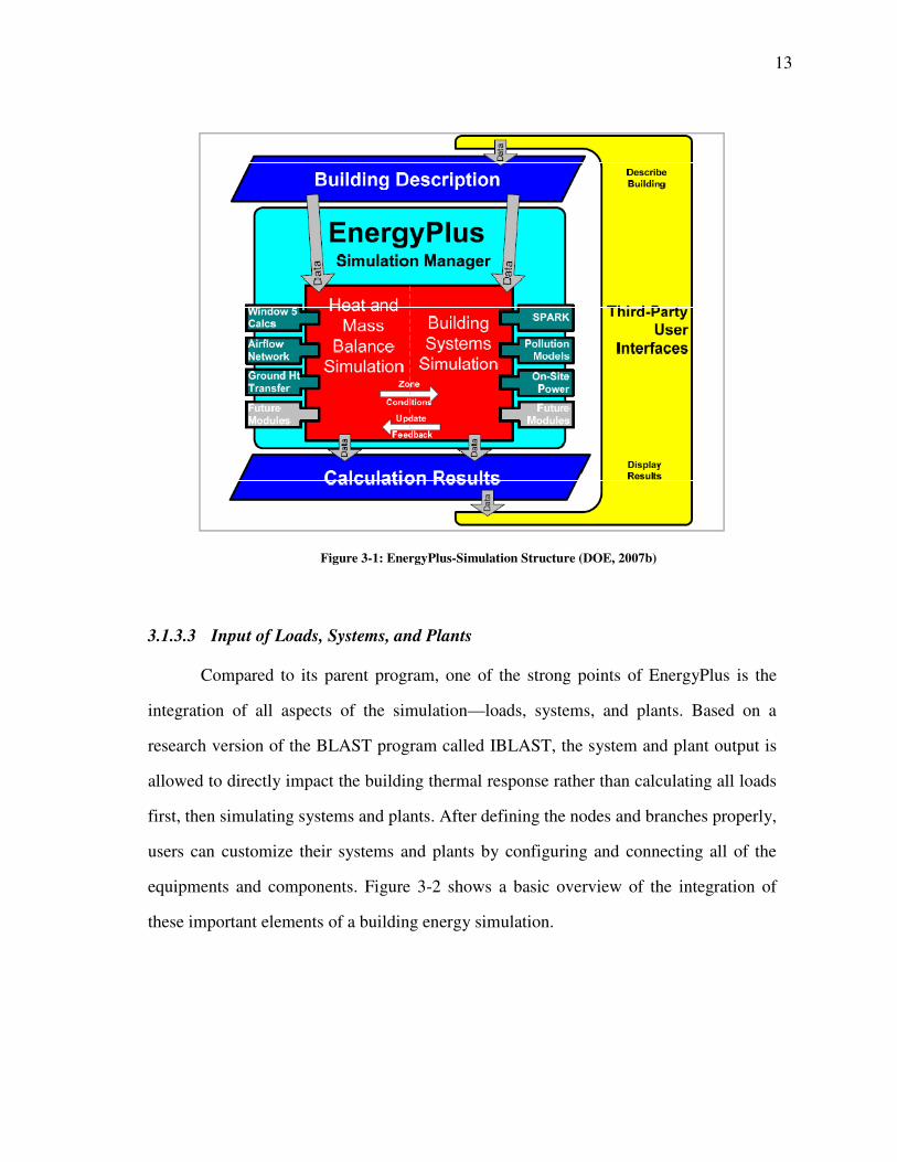
and a big picture view of how future work can impact the program. Figure 3-1 shows the
structure of EnergyPlus.
13
Figure 3-1: EnergyPlus-Simulation Structure (DOE, 2007b)
3.1.3.3 Input of Loads, Systems, and Plants
Compared to its parent program, one of the strong points of EnergyPlus is the
integration of all aspects of the simulation—loads, systems, and plants. Based on a
research version of the BLAST program called IBLAST, the system and plant output is
allowed to directly impact the building thermal response rather than calculating all loads
first, then simulating systems and plants. After defining the nodes and branches properly,
users can customize their systems and plants by configuring and connecting all of the
equipments and components. Figure 3-2 shows a basic overview of the integration of
these important elements of a building energy simulation.

14
Figure 3-2: EnergyPlus Internal Elements (DOE, 2007b)
A module developer is someone who is going to add to the simulation
capabilities of EnergyPlus. A module is a Fortran 90/95 programming construct that can
be used in various ways. In EnergyPlus, its primary use is to segment a rather large
program into smaller, more manageable pieces. Each module is a separate package of
source code stored on a separate file. The entire collection of modules, when compiled
and linked, forms the executable code of EnergyPlus.
The “Surface Heat Balance Manager” is driven to calculate the heat transferring
through the building envelop. It includes “Sky Model Module”, “Shading Module”,
“Daylighting Module”, “Window Glass Module” and “CTF Calculation Module”. “Sky
Module” is designed to calculate the sky radiation. In EnergyPlus, the calculation of
diffuse solar radiation from the sky incident on an exterior surface takes into account the
anisotropic radiance distribution of the sky. “Shading Module” is designed for shading
and sunlit area calculations. When assessing heat gains in buildings due to solar
radiation, it is necessary to know how much of each part of the building is shaded and
15
how much is in direct sunlight. “Daylighting Module”, in conjunction with the thermal
analysis, determines the energy impact of daylighting strategies based on analysis of
daylight availability, site conditions, window management in response to solar gain and
glare, and various lighting control strategies. “Window Glass Module” is considered to
be composed of four components: glazing, frame, divider and shading device.
The “Air Heat Balance Manager” is driven to solve the heat balance problems in
the air flow in the building. It includes “AirFlow Network Module”. It includes five
segments: infiltration, ventilation, mixing, cross mixing and earth tube.
The “Building Systems Simulation Manager” is developed for HVAC systems
applied in the building. It includes “AirLoop Module”, “Zone Equip Module”, “Plant
Loop Module”, “Condenser Loop Module” and “PV Module”. “AirLoop Module” is
developed to calculate the mass and heat transfer in the primary air loop (i.e.,
representing the supply side of the loop). “Zone Equip Module” is developed to calculate
the mass and heat transfer in the zone equipment (e.g., terminal VAV box). “Plant Loop
Module” and “Condenser Loop Module” are developed to calculate the heat and mass
transfer between the energy demand side and the plant side. Typically, the central plant
interacts with the systems via a fluid loop between the plant components and heat
exchangers, called either heating or cooling coils.
In the EnergyPlus input file, detailed information of HVAC systems is required.
Zone load information includes number of people, lighting and equipment intensity.
System information includes configuration of air loop and water loop. During this
configuration, nodes and branches should be carefully connected to complete the loops
for both air and water. Moreover, detailed information of coils, pumps, connecters,
splitters, mixers and controllers should also be configured.

16
3.1.3.4 Output Files of EnergyPlus
This section is intended to give a brief introduction for the various output files
produced by EnergyPlus. The two scripts that are distributed with EnergyPlus are: EPL-
Run.bat (which is used by the EP-Launch program) and RunEPlus.bat (which can be
used from the command line). The RunEPlus batch file can also be used to string
together several runs such as usually termed “batch processing”. In renaming the files
created by the program or its post-processing program(s), usually the file extension will
be retained. For output purposes, the most important files to understand are the
eplusout.eso, eplusout.mtr and eplusout.err files. The first two are manipulated with the
ReadVarsESO post processing program. The latter will contain any critical errors that
were encountered during the run.
3.1.4 Description of the Simulation Model
The calibrated model was created to represent the initial system of the building
being simulated. For this model, load information, zoning and system operation
schedules were created to represent the current operating conditions. The envelope
materials data and their U-values were provided by the facility office. Figure 3-3 is the
picture of the case-study building and the model created by the simulation software
DesignBuilder V1.0 (DesignBuilder Software Ltd. 2007)

17
Figure 3-3: Simulation Model
To simplify the research while still achieving the research objective, only one
terminal reheat box was assigned to each zone. In the actual case-study building, each
zone has several boxes. To calibrate the model, 2006 hourly weather data for College
Station, Texas was used and the simulation results were compared against the measured
energy use. Coefficient of variance of the root mean square error CV(RMSE) for whole
building electricity, chilled water consumption and hot water consumption as well as the
mean bias errors (MBE) was used as an overall indicator to fine-tuned the simulation to
an acceptable level.
3.1.5 Location and Weather File
The simulated building is located in the research park of Texas A&M University,
College Station, Texas (30.61°N, 96.32°W). Real weather files for College Station,
Texas were used for calibration. According to ASHRAE definition, it is located in a hot
and humid area. The average daily outdoor dry bulb temperature of 2006 ranges from
34°F to 88°F and relative humidity is from 34% RH to 94% RH. The annual average

18
temperature is 60.8°F and the annual average relative humidity is 65% RH. Figure 3-4
is daily average OAT and outdoor humidity ratio for College Station in 2006.
Figure 3-4: OAT and Outdoor Relative Humidity for College Station 2006
3.1.6 Zone Loads
3.1.6.1 Building Envelope Information
The external envelope of the building is constructed of concrete walls, glass
walls and single-panel glass windows. The internal walls separate the conditioned
zones into exterior areas and interior areas.
19
There are two types of exterior walls. One is an opaque wall and the other is
glass block. The opaque wall is made up of 4-inch brick, 3-inch polystyrene, 4-inch
concrete block as well as ½ inch gypsum paste. The overall U-value of the exterior wall
is 0.062 Btu/ ft²·F°·h. The glass block has a U-value of 0.89 Btu/ ft²·F°·h. For the interior
walls, a ¾ inch gypsum board was assigned with an R-value of 0.67 ft²·F°·h/Btu. The
drop ceilings are acoustic tiles with an R-value of 3.7 ft²·F°·h/Btu. Roof construction is
combined with ½ inch roof gravel, 3⁄8 inch built-up roofing, polyurethane insulation and
¾ inch wood. The U-value of roof is 0.05 Btu/ ft²·F°·h. The floor construction is 6-inch
lightweight concrete with a U-value of 0.05 Btu/ ft²·F°·h. The glass for the windows is
single-pane, tinted, with a U-value of 1.09 Btu/ ft²·F°·h. The ratio between windows to
external walls of this building is 14%.
3.1.6.2 Zoning
All of the floors are divided into two zones (i.e., exterior and interior). The
interior zone is defined as a barrier 15 ft away from the exterior wall in each direction.
Figure 3-5 shows the detailed zoning plan for each floor. The spaces between the
internal walls and external walls are defined as exterior areas.

20
(a) First Floor
(b) Second Floor
(c) Third Floor
Figure 3-5: Building Zoning
21
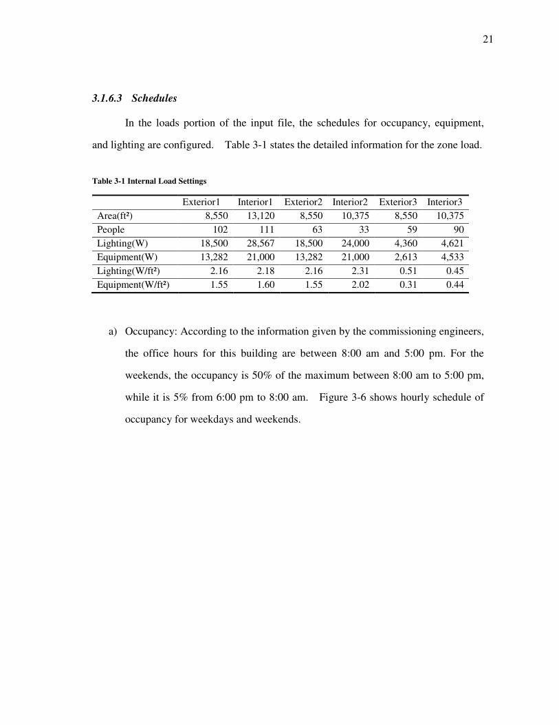
3.1.6.3 Schedules
In the loads portion of the input file, the schedules for occupancy, equipment,
and lighting are configured. Table 3-1 states the detailed information for the zone load.
Table 3-1 Internal Load Settings
Exterior1 Interior1 Exterior2 Interior2 Exterior3 Interior3
Area(ft²) 8,550 13,120 8,550 10,375 8,550 10,375
People 102 111 63 33 59 90
Lighting(W) 18,500 28,567 18,500 24,000 4,360 4,621
Equipment(W) 13,282 21,000 13,282 21,000 2,613 4,533
Lighting(W/ft²) 2.16 2.18 2.16 2.31 0.51 0.45
Equipment(W/ft²) 1.55 1.60 1.55 2.02 0.31 0.44
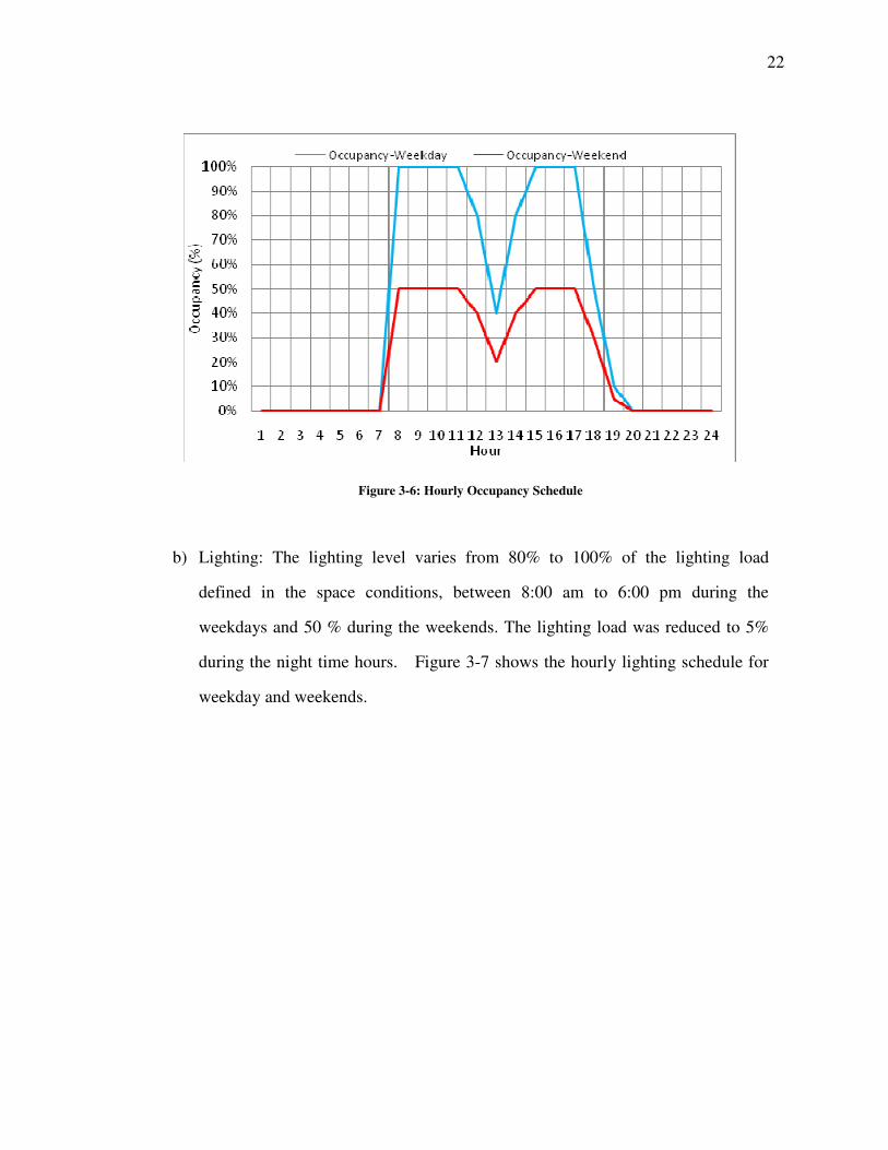
a) Occupancy: According to the information given by the commissioning engineers,
the office hours for this building are between 8:00 am and 5:00 pm. For the
weekends, the occupancy is 50% of the maximum between 8:00 am to 5:00 pm,
while it is 5% from 6:00 pm to 8:00 am. Figure 3-6 shows hourly schedule of
occupancy for weekdays and weekends.
22
Figure 3-6: Hourly Occupancy Schedule
b) Lighting: The lighting level varies from 80% to 100% of the lighting load
defined in the space conditions, between 8:00 am to 6:00 pm during the
weekdays and 50 % during the weekends. The lighting load was reduced to 5%
during the night time hours. Figure 3-7 shows the hourly lighting schedule for
weekday and weekends.

23
Figure 3-7: Hourly Lighting Schedule
c) Equipment: The Equipment load varied from 50% to 100% of the full load
defined in the space conditions, between 8:00 am to 9:00 pm. For the remainder
of the time it was assumed to be at 50%. On weekends, the equipment load
remained at 50% during daytime and 30% during the evening hours. Figure 3-8
shows the hourly equipment schedule for weekday and weekends.

24
Figure 3-8: Hourly Equipment Schedule
3.1.7 HVAC System
There are three (3) SDVAV air-handling units serving the building. In all three
units, the outside air is mixed with the return air and is then cooled down through the
cooling coil to the SAT setpoint and reheated, if necessary, at the terminal box to
maintain the zone temperature setpoint. The diagram of a typical SDVAV unit with
terminal reheat boxes is shown in Figure 3-9.
In this system, the preheat coil warms the mixed air to the preheat setpoint to
protect the cooling coil from freezing. Chilled and hot water is provided by the campus
central plant. In this simulation, purchased chilled water and hot water were used to
account for the heating and cooling loads. No chillers or boilers were simulated. This
configuration was chosen to match the measured chilled and hot water from the physical
plant.

25
Figure 3-9: Diagram of SDVAV with Terminal Reheat
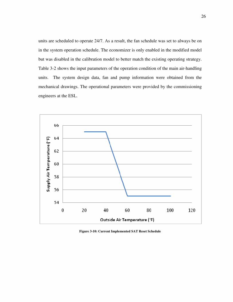
3.1.7.1 HVAC System Operation Description
In the system control objects, the preheat temperature is set at 45°F. There is a
linear reset schedule for the SAT implemented to the three units under the existing
operation. Figure 3-10 illustrates the current reset schedule for the SAT. When the
outside air is above 60°F, the SAT is set to a constant number as 55°F. The SAT can be
raised to a higher temperature when the cooling load decreases as the OAT drops. When
the OAT is below 40°F, the SAT is fixed to 65°F. When the ambient temperature is
between 60°F and 40°F, the SAT increases from 55°F to 65°F linearly.
The minimum outside air control method was a proportional minimum, which
means it will be kept at a constant ratio with respect to the total flow rate. The cooling
design flow method was set as “flow/system”, which means the program will use the
user input flow rate as the system flow rate instead of the program calculated design
value. Due to the specific requirement for the laboratories in the simulated building, the
26
units are scheduled to operate 24/7. As a result, the fan schedule was set to always be on
in the system operation schedule. The economizer is only enabled in the modified model
but was disabled in the calibration model to better match the existing operating strategy.
Table 3-2 shows the input parameters of the operation condition of the main air-handling
units. The system design data, fan and pump information were obtained from the
mechanical drawings. The operational parameters were provided by the commissioning
engineers at the ESL.
Figure 3-10: Current Implemented SAT Reset Schedule

27
Table 3-2: System Setting Parameters
Item Unit AHU1 AHU2 AHU3
Serving Floor Area ft² 21,670 18,925 18,925
Design Flow Rate cfm 22,050 21,610 20,160
Design Min OA Flow Rate cfm 3,950 2,070 1,900
OA flow method
Proportional Minimum
Min Flow Ratio
0.15 0.15 0.15
Preheat Set Point °F 45 45 45
Precool design humidity ratio lb-H2O/lb-air 0.008 0.008 0.008
Cooling Design Setpoint °F 55 55 55
Cooling design air flow method
flow/system
Economizer
No Economizer
Fan Type
Simple: Variable Volume
Fan Delta Pressure in H2O 4.5 4.15 4.05
Fan Total Efficiency
0.7 0.7 0.7
Fan Schedule
Weekday: Always On / Weekend: 6:00-22:00
3.1.7.2 Zone Equipment Operation Description
In EnergyPlus, the user must define equipment for each zone; including terminal
reheat boxes, heating coils, air distribution units, thermostats as well as humidity sensors
if humidity control is required. In addition, the zone control strategy can also be
customized. Table 3-3 summarized the input control parameters for terminal reheat
boxes used in the simulation. The outside air flow rate, maximum design flow rate and
minimum flow rate were kept the same as the design value. The design value matches
the measured data according to the commissioning engineers at the ESL. The zone
thermostat control method was a dual setpoint with a deadband. Both the heating and
cooling setpoints can be scheduled for any given time period. The cooling setpoint is
74°F during occupied hours and 79°F during unoccupied hours. The heating setpoint is
70°F during occupied hours and 61°F during unoccupied hours. The operation schedule

28
and zone temperature setpoint information was provided by the commissioning
engineers at the ESL.
Table 3-3: Load Ratio Schedule
Unit Exterior1 Interior1 Exterior2 Interior2 Exterior3 Interior3
OA Flow Rate cfm 1,778 2,172 1,040 1,030 950 950
Min cfm Ratio
0.15 0.15 0.15 0.15 0.15 0.15
Zone Max
Relative Humidity %RH
No Humidity Control Implemented
Zone Cooling
Setpoint(Occ) °F 74 74 74 74 74 74
Zone Cooling
Setpoint(Unocc) °F 79 79 79 79 79 79
Zone Heating
Setpoint(Occ) °F 70 70 70 70 70 70
Zone Heating
Setpoint(Unocc) °F 61 61 61 61 61 61
Zone Thermostat
Control Method Dual Setpoint with Deadband
3.1.7.3 Plant Operation Description
The chilled water and hot water of the simulated case-study building are
provided by the campus central plant. There is one chilled water pump and one hot water
pump in the building to provide enough pressure for the building. Hence, in EnergyPlus
purchased energy system was configured in the simulation input file. The heating and
cooling systems were set to always be available during the year. The hot water supply
temperature setpoint was set to 160°F, and the chilled water supply temperature was set
at 43°F.
29
3.2 Simulation Output Analysis and Calibration
3.2.1 Need for Calibration
Historically, the inputs for energy simulations of commercial buildings have been
based on design data. The experience of the researchers and engineers who have
performed hundreds of energy simulations indicates that differences of 50% or more
between simulation results based on design data and measured consumption are not
unusual. These errors are not thought to be due to errors in the simulation software itself,
but to errors in the input assumptions for a particular building, due to misunderstanding
of the building’s design or to the differences between design and as-built conditions or
operations. Consequently, many organizations and individuals have developed
procedures to adjust the inputs used to “calibrate” a simulation so the simulated results
more closely match measured consumption.
For commercial buildings, the variables of interest are chilled water (CHW) and
hot water (HW) usage and the whole building electricity (WBE). For a building that is
being supplied chilled water and hot water, these three variables can often satisfy the
purposes of calibration.
3.2.2 Calibration Method and Calibration Result
In this thesis, the approach to calibrated simulation is based on the previous work
by the Energy Systems Laboratory (ESL) for several years in different applications.
The method is based on a unique graphical representation of the difference between the
simulated and measured performance of a building, referred to as a “Calibration
Signature”. For a given system type and climate, a graph of this difference has a
characteristic shape that depends on the reason for the difference. Calibration signatures
have been used for diagnostics and prediction of the savings from commissioning

30
projects. The process is efficient enough that it has been used to predict savings from
commissioning measures in dozens of buildings in a variety of contracted
commissioning jobs. There are several metrics used in evaluating whether or not a
simulation is sufficiently calibrated, or in comparing two possible calibration
adjustments. Three parameters (i.e. MBE, RSME, CV(RSME)) are used to evaluate the
simulation results.
3.2.2.1 Mean Bias Error (MBE)
The mean bias error (MBE) is a measure of the sum of errors in a non-
dimensional format. The total difference between the two sets of data for each hour or
day is then divided by the total number of data points minus the number of regression
variables. This will give the mean bias or the mean of the residuals. This value divided
by the mean of the model will give the MBE in percentage form. Mathematically it is
given by:
3-1
where n is the number of data points. With the MBE, positive and negative errors cancel
each other out, so the MBE is an overall measure of how biased the data is. The MBE
is also a good indicator of how much error would be introduced into annual energy
consumption estimates, since positive and negative daily errors are cancelled out.
3.2.2.2 Root Mean Square Error (RMSE)
Root Mean Square Error is defined as:
MBE= ×100% ∑( Esim-Emea )
n×Emea,ave

31
2
2
−
−∑n
)E(E measim
3-2
where n is the number of data points. The RMSE is a good measure of the overall
magnitude of the errors. It reflects the size of the errors and the amount of scatter, but
does not reflect any overall bias in the data.
A simulation with a small RMSE, but with a significant MBE, might indicate an
error in simulation inputs. A simulation with a large RMSE but a small MBE might have
no errors in simulation inputs, but building performance may reflect some other un-
modeled behavior (such as occupant behavior) that is difficult to simulate, or it may have
significant input errors.
3.2.2.3 Coefficient of Variance of Root Mean Square Error CV(RMSE)
The coefficient of variation of the root mean square error (CV(RMSE)) is
essentially the non-dimensional form of the RMSE. It is obtained by dividing the RMSE
by the mean of the data set, which is being used as the benchmark. It is given by
3-3
This value depicts how well the simulation model fits the measured data. The
main aim of calibrating a simulation model is to lower this value. The CV(RMSE) and
MBE have been used extensively in the calibration process of building energy
simulation models. For the purpose of better calibrating a simulation model to the
measured data, the use of hourly CV(RMSE) and MBE can be justified. The reason is
that in using daily or monthly percentage differences, the dissimilarities between the
model and the actual conditions are overlooked, because over longer periods these
changes tend to balance out. So it cannot be said with certainty that the resulting model
CV(RMSE)=
RMSE
Emea,ave
RMSE=
32
is a true depiction of the building operations. Nevertheless, daily data is used in this
research for calibration limited to the lack of hourly data.
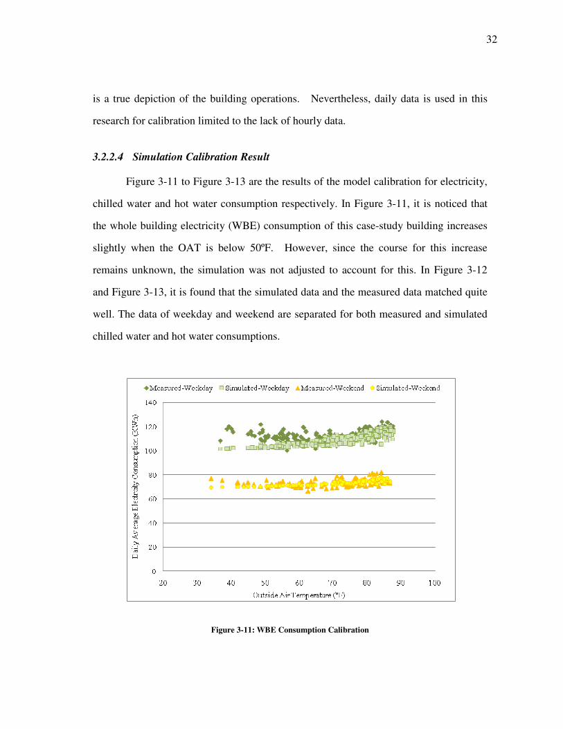
3.2.2.4 Simulation Calibration Result
Figure 3-11 to Figure 3-13 are the results of the model calibration for electricity,
chilled water and hot water consumption respectively. In Figure 3-11, it is noticed that
the whole building electricity (WBE) consumption of this case-study building increases
slightly when the OAT is below 50ºF. However, since the course for this increase
remains unknown, the simulation was not adjusted to account for this. In Figure 3-12
and Figure 3-13, it is found that the simulated data and the measured data matched quite
well. The data of weekday and weekend are separated for both measured and simulated
chilled water and hot water consumptions.
Figure 3-11: WBE Consumption Calibration

33
Figure 3-12: Chilled Water Consumption Calibration
Figure 3-13: Hot Water Consumption Calibration

34
The only change in the input file from the design configuration was the minimum
air flow ratio. In the calibrated simulation, the minimum air flow ratio was adjusted to
15% to match the measured conditions. In the remaining of this thesis, a value of 30%
was assigned. Table 3-4 shows the results of calibration.
Table 3-4: Summary of Calibration Results
Measured Energy Use Simulated Energy Use CV(RMSE)% MBE%
WBE 94kWh 98kWh 9.54 1.84
CHW 378KBtu/hr 376KBtu/hr 5.71 -0.24
HW 88KBtu/hr 62KBtu/hr 41.60 -4.53
3.3 Optimized SAT Reset Schedule
This section contains the methodology and results from the simulation including
the optimized SAT reset schedule. An example is provided in the first section to
demonstrate the method of how to simulate the most cost effective SAT schedule.
3.3.1 Optimal SAT Reset and Cost Comparison
The traditional reset schedule is typically implemented as a linear function with
respect to the OAT. Figure 3-14 shows the current as well as the optimal reset schedule
for the simulated building.

35
Figure 3-14: Comparison of Linear and Optimal SAT Reset Schedules
Figure 3-15 and Figure 3-16 show the comparison of energy consumption and
costs among the optimal SAT reset schedule, the linear SAT reset schedule and non-
reset SAT schedule. Table 3-5 shows details of the fan electricity, cooling and heating
costs for three SAT reset schedules. Compared with the conventional linear reset
schedule, the optimized reset schedule can save electricity, cooling and heating
consumption by 18.59%, 3.44% and 2.47% respectively while the total costs can be
reduced by 6.23% on an annual basis. If the optimal supply air temperature reset
schedule is compared with a constant supply air temperature setpoint of 55 °F, these
savings will reach 11.80%, 3.84% and 34.78% for electricity, cooling and heating
respectively including an 8.44% total cost savings.

36
Figure 3-15: Annual Energy Consumption Comparison
Figure 3-16: Comparison of Annual Total Cost
Table 3-5: Cost Comparison for Three SAT Schedules
Energy Consumption Savings (%)
Opt SAT LinearSAT Const55 OptSAT vs LinearSAT OptSAT vs Const55
Fan Electricity $1,339.71 $1,645.73 $1,518.96 18.59 11.80
CHW $6,217.45 $6,438.95 $6,465.93 3.44 3.84
HW $610.31 $625.74 $935.53 2.47 34.76
Total Cost $8,167.47 $8,710.42 $8,920.42 6.23 8.44

37
3.3.2 Typical Optimal SAT Reset Schedule
To facilitate the discussion of an example simulation, a typical optimal supply air
temperature is divided into five zones. Ten critical temperatures are also defined. Table
3-6 shows the definition of those ten critical temperatures. Figure 3-17 shows the typical
optimal supply air temperature reset schedule.
Figure 3-17: Optimized Supply Air Temperature with and without Humidity Control
For a typical optimized supply air temperature with humidity control, five zones
are defined and analyzed in the rest of this research.
• Zone 1: TOA ≤ TOA,low
• Zone 2: TOA,low< TOA ≤ TOA,lhum
(TOA,low,TSA,high)
(TOA,high,TSA,low)
(TOA,hhum,TSA,hum)
(TOA,eco,TSA,eco)
(TOA,lhum,TSA,mid)
(TOA,lhumTSA,hum)

38
• Zone 3: TOA,lhum< TOA ≤ TOA,hhum
• Zone 4: TOA,hhum< TOA ≤ TOA,high
• Zone 5: TOA>TOA,high
Table 3-6: List of Critical Temperatures
Name Definition Name Definition
TOA,low
Outside air temperature at which a constant high supply air temperature can be implemented.
TSA,high Supply air temperature high limit.
TOA,lhum
Outside air temperature at which outdoor humidity becomes high. The optimal supply air temperature begins to be override to a low value for humidity control.
TSA,mid
Supply air temperature when outdoor humidity is high and optimal supply air temperature begins to be override to a low value.
TOA,lhum Same as above. TSA,hum
A constant supply air temperature to assure the humidity level in the conditioned space is below 65%RH.
TOA,hhum Outside air temperature at which supply air temperature can be increased from TSA,hum.
TSA,hum Same as above.
TOA,eco Outside air temperature at which economizer is enabled.
TSA,eco Supply air temperature when economizer is enabled.
TOA,high
Outside air temperature at which cooling energy consumption is significant and heating load is negligible.
TSA,low
Supply air temperature when the cooling load is at its peak and air with constant low temperature can be sent into conditioned space.
3.3.2.1 Zone 1: TOA ≤ TOA,low
When OAT is lower than a certain temperature (TOA,low), the heating load is
significant in the exterior area and the supply air temperature can be set at the high limit
(TSA,high) to minimize the reheat consumption in the terminal boxes. Meanwhile, interior
area still needs cooling. As a result, the SAT should still be kept at a certain level to

39
remove the heat gain in the interior area. In this research the high limit is set at 65°F,
because if the supply air temperature is above this value, it is unable to remove zone
cooling load.
3.3.2.2 Zone 2: TOA,low<TOA ≤ TOA,lhum
In this zone, the space heating requirement is decreasing with the increase in the
OAT. As a result, the cost efficient supply air temperature is decreasing when the
ambient temperature increases. In this range of OAT, the economizer is enabled, which
means free cooling is being used and the mechanical cooling is reduced. In addition,
outdoor air is relatively dry. In this zone, the optimized SAT reset is the same for both
humidity control and non-humidity control situation.
The SAT is supposed to decrease from TSA,high when the OAT is TOA,low to TSA,mid
or when the OAT is TOA,lhum. In addition, the TOA,low and the TOA,lhum are dependent on
several factors: building location, weather conditions, minimum air flow rate, etc.
3.3.2.3 Zone 3: TOA,lhum<TOA ≤ TOA,hhum
In this zone, the outside air is very humid and the SAT should be lowered to
control the humidity at the cost of simultaneous heating and cooling. The supply air
temperature is set as low as is needed to control the relative humidity in the conditioned
spaces and as high as possible to minimize over-cooling. The TOA,lhum and the TOA,hhum
are the two points where the optimal supply air temperature resets for humidity and non-
humidity control meet. TOA,lhum is the critical temperature where supply air temperature
should be lowered to dehumidify the mixed air while on the opposite side, TOA,hhum is
where the most cost efficient SAT is low enough to control the humidity. Both the
TOA,lhum and the TOA,hhum are related to location and weather conditions. In this particular
40
case, TOA,lhum is 55ºF while TOA,hhum is 74ºF. TSA,mid and TSA,hum are different for different
operation conditions which will be discussed later.
3.3.2.4 Zone 4: TOA,hhum<TOA≤ TOA,high
In this zone, the optimal SAT declines from TSA,hum to TSA,low while the OAT
increases from TOA,hhum to TOA,high. During this period, the cooling load is climbing
swiftly with the rise of the OAT while the heating load is neglected. The optimized SAT
decreases as long as overcooling is avoided and it is low enough to control the humidity
below 65 %RH in the conditioned space. Both the TOA,hhum and the TOA,high are affected
by weather conditions and operation scenarios.
3.3.2.5 Zone 5: TOA>TOA,high
When the OAT is above a specific temperature (TOA,high), the zone cooling load is
dominant and no heating is called from the conditioned zones. As a result, the SAT can
be lowered to a constant value where no over-cooling will occur. In this research, this
low temperature is defined as TSA,low, and cut off at 50°F which is the limit established
by the capacity of chillers. Both the TOA,high and the TSA,low change with varying
operation conditions.
41
4 . DIFFERENT OPERATING CONDITIONS
4.1 Influence of Minimum Flow Ratio
This section analyzes the changes of the optimal SAT reset driven by changing
minimum air flow ratio. To analyze this, the minimum flow ratio has been changed from
15% to 30%, 50% and 100% while all the other input parameters were kept the same.
Notice that at the 100% minimum air flow ratio, the system cooperates as a constant
volume unit. Figure 4-1 shows the four temperature curves of the four different
minimum flow ratios when the internal peak load is around 4.0W/ft2, exterior area
account for 42% of the total floor area and cooling price was $5.5/MMBtu while heating
cost was $12.82/MMBtu.
The results show that a proper minimum flow should be applied in a SDVAV
system. It should be high enough to meet ventilation requirement and low enough to
prevent over-cooling and reheat. A high minimum flow is likely to produce extra cooling
or heating energy. For example, when the outside air is 75°F, a 15% air flow at 55°F can
exactly remove the cooling load from the space. However, if the minimum flow is set at
30%, 15% extra cooling energy is going to be sent to the zone which results in 15%
over-cooling as well as a 15% reheat. In this case, if the SAT is increased to a higher
value, for instance, 57°F, overcooling can be avoided. As a result, the SAT reset should
be higher for a higher minimum flow setpoint if other operation parameters are kept the
same.

42
Figure 4-1: SAT Reset Schedules for Different Minimum Flow Ratios
4.2 Influence of Exterior Zone Area Ratio
The cooling and heating loads for the exterior zone vary significantly during the
year depending on outside conditions. They call for a large amount of cooling in the
summer and heating in the winter. Meanwhile, the load for the interior zone remains
quite stable year round, requiring cooling to fulfill the zone thermal comfort
requirements. Different zoning methods may result in different load distributions and
different optimized control strategies. Hence, it is necessary to evaluate the impact of
the zone loads on the SAT reset. Figure 4-2 and Figure 4-3 show system cooling and
heating loads with different exterior zone area ratios. In this research, the exterior zone
43
area ratio was defined as the ratio of exterior zone area to the total floor area. It was
adjusted from 0% to 22%, 42% and 100% in steps where 100% exterior zone area ratio
equals to one single zone for the entire floor. The results show that both the cooling and
heating loads for the system are lower for a larger exterior zone area ratio. The only
exception is that when the OAT is higher than the zone setpoint temperature. During this
condition, the cooling load is lower for the interior zone than the exterior zone. The
reason is that for the unit serving the exterior zone, the cooling load in the exterior zone
is influenced by the heat transfer through the building envelope. When the OAT is lower
than the setpoint temperature, the internal heat gain by the occupants, equipment and
lights compensate the heat loss through the envelope which results in a lower heating
load in the exterior zone. As a result, for large exterior zones, more internal heat gain
can contribute to counteract the heat loss from the envelope, which results in less heating
load in the exterior zone. Since the internal load in the exterior zone are counteracted by
the heat loss through the envelope when the OAT is less than the setpoint temperature,
the cooling loads will be reduced in the interior zone. Here, minimum flow is 30%,
internal load is 4.0 W/ft2 and the heating/cooling energy price ratio is 2.33. Figure 4-4
shows the results of the different SAT reset schedules for different exterior zone area
ratios. The result shows that the larger the exterior zone area is, the higher SAT should
be set in the heating season and lower SAT in the cooling season. For example, if it is an
exterior area only unit, TSA,high can be up to 65°F while TSA,high is only 62°F for an
interior area only unit. The reason is that the heating load takes priority in the exterior
zone area while in the interior zone area only a cooling load exists. When the OAT is
below 28°F, the large variations for the system loads shown in Figure 4-4 is due to the
solar radiation and small number of hours for these OAT bins in Houston.

44
Figure 4-2: System Cooling Loads for Different Exterior Zone Area Ratios
Figure 4-3: System Heating Loads for Different Exterior Zone Area Ratios

45
Figure 4-4: SAT Reset Schedules for Different Exterior Zone Area Ratios
4.3 Influence of Internal Load
In this section, the impact of the internal loads will be discussed. Similar to the
previous analysis, all the other operation conditions were kept the same. Only the
internal load was increased from 3.5 W/ft2 to 4.0 W/ft2 and 4.5 W/ft2.

46
Figure 4-5: SAT Reset Schedules for Different Internal Loads
Figure 4-5 shows the three SAT curves for the three internal load intensities
when the exterior zone area ratio was set to 42%, minimum flow ratio was 30% of the
total flow and heating/cooling price ratio was 2.33. From the results, it is reasonable to
conclude that a higher internal load should result in a lower SAT. In this specific case,
the optimized SAT was lowered by 1°F when the internal load increased by 0.5 W/ft².
This would indicate that when the internal load increases, the SAT should be decreased
due to the additional cooling load.
47
4.4 Influence of EnergyPrices
The energy price is another important factor in determining the optimized SAT
reset. The price ratio is defined as:
4-1
In this study, three price ratios were investigated including 1.17, 2.33 and 3.50.
Figure 4-6 shows the different SAT reset schedules for the different price ratios. The
results show that the higher the price ratio is, the higher the SAT should be set in the
heating season. If the price for hot water goes up, the cost on the heating side should take
priority reset because more money can be saved if the SAT is increased and less heating
energy is consumed. On the contrary, if the gas price or the heating energy price
decreases, electricity should take priority for cost efficiency which indicates a lower
SAT. Notice that there is no difference for the three SAT reset schedules when the OAT
is above TOA,lhum. When the OAT ranges from TOA,lhum and TOA,hhum, the SAT should be
lowered to control the space humidity and when the OAT is above TOA,hhum, no heating is
required for the system. As a result, the heating price has no impact on the SAT reset
schedule when the OAT is above TOA,lhum.
Price Ratio=
Heating Energy Cost($/MMBtu)
Cooling Energy Cost($/MMBtu)

48
Figure 4-6: SAT Reset Schedules for Different Price Ratios

49
5 . CONCLUSIONS
Determining the optimal SAT is a complex process which is influenced by
various factors, such as weather condition, minimum air flow rate, exterior area ratio,
internal load and utility price. A guideline for determination of a cost efficient SAT for
single duct VAV units is drawn in this research. Furthermore, a brief introduction on
how to adjust SAT reset schedule with different operation scenarios is presented.
5.1 Five Zones for SAT Reset Schedule
The most cost efficient optimal SAT can be divided into five zones with respect
to ambient temperature. To simplify the discussion, some critical temperatures are
defined in this research as shown in Figure 5-1 and the detailed definition can be found
in the former sections.
• Zone 1: TOA ≤ TOA,low
• Zone 2: TOA,low< TOA ≤ TOA,lhum
• Zone 3: TOA,lhum< TOA ≤ TOA,hhum
• Zone 4: TOA,hhum< TOA ≤ TOA,high
• Zone 5: TOA>TOA,high

50
Figure 5-1: Typical Optimized SAT
5.1.1 Zone One: TOA ≤ TOA,low
In the first zone, when the OAT is equals to or below TOA,low, the zone cooling
load is very small and significant heating energy is required. Therefore, the SAT can
be set as a constant value, TSA,high.
5.1.2 Zone Two: TOA,low< TOA ≤ TOA,lhum
In the second zone, when the OAT is above TOA,low and equals to or below
TOA,lhum, the zone heating load is decreasing and the SAT should decrease from TSA,high
to TSA,hum while the OAT increases from TOA,low to TOA,lhum.
(TOA,low,TSA,high)
(TOA,lhum,TSA,hum)) (TOA,hhum,TSA,hum)
(TOA,lhum,TSA,mid)
(TOA,high,TSA,low)
1 2 3 4 5
TSA,high
TSA,mid
TSA,hum
TSA,low
TOA,low TOA,lhum TOA,hhum TOA,high

51
5.1.3 Zone Three: TOA,lhum< TOA ≤ TOA,hhum
When the OAT ranges from TOA,lhum and TOA,hhum and outdoor humidity level is
high, the SAT is required to be kept at a low value, TSA,hum, even at the cost of extra
energy consumption in the form of reheat energy to maintain zone humidity ratio below
65 %RH.
5.1.4 Zone Four: TOA,hhum< TOA ≤ TOA,high
When the OAT continues to increase, the cooling load increases rapidly and the
SAT should decrease so that less fan power is consumed in the air-handling unit. In
other words, when the OAT increases from TOA,hhum to TOA,high, the SAT should decrease
from TSA,hum to TSA,low. Note that depending on different building conditions, if
minimum air flow ratio is high above a certain level, TOA,high may become an infinitive
large number and SAT should keep at TSA,hum to control zone humidity.
5.1.5 Zone Five: TOA>TOA,high
The last zone indicates an area where the cooling load is very large and the SAT
can be set at a constant low value, TSA,low.
5.2 Influence of Different Operating Conditions
Four key influencing operation parameters have been analyzed in this study and
Table 5-1 summarizes the guidelines of the adjustment of the optimized SAT reset
schedule, including:
1) A high minimum flow ratio indicates a high SAT for both the heating and
cooling mode.
2) A high exterior area zone ratio results in a high SAT in the heating mode and a
low SAT in the cooling mode.

52
3) A high internal load should have a low SAT in both the heating and cooling
seasons.
4) A high electricity cost implies a low SAT while a high heating price implies a
high SAT setpoint.
Table 5-1: Adjustment of Critical Temperatures for Various Conditions
Minimum Flow↑ Exterior Area↑ Internal Load↑ Price Ratio↑
TOA,low ↑ ↑ ↓ ↑
TSA,high ↑ ↑ ↓ ↑
TOA,lhum − − − −
TSA,mid ↑ − ↓ ↑
TOA,hhum ↑ ↓ ↓ −
TSA,hum − − − −
TOA,high ↑ ↓ ↓ −
TSA,low ↑ ↓ ↓ −
5.3 Recommendations for Further Research
The optimization of the SAT is a complex issue that is related to many factors.
Unfortunately, it is difficult to discuss and analyze all the influencing factors in a single
analysis. This research has provided a weather bin method for optimizing the SAT.
Moreover, four major influencing factors (minimum flow ratio; exterior area zone ratio;
internal load and energy prices) have been individually investigated. Nevertheless,
further research for some other variables could be developed. To name a few, five
considerations were carried out below as suggestions.

53
5.3.1 Installed Plant Equipment
In this research, the purchased chilled water and hot water were used to meet the
building cooling and heating requirement. As a result, a constant chiller and boiler
efficiency was assumed while in a real case the chiller efficiency will be higher in the
cold season and the boiler efficiency will be higher in the hot season. In addition, the
electricity consumed by the chillers, boilers, cooling towers and pumps should also be
considered in the calculation of the total cost when determining the optimal SAT reset
schedule.
5.3.2 Different Zone Temperature Setpoint
There are many operation parameters that may influence the reset strategy of the
SAT. In this research, four major factors were being discussed while the zone
temperature setpoints were locked at one constant value. Therefore, it might be desirable
to find out what other adjustments to the SAT should be made if the zone temperature
setpoint is changed.
5.3.3 Different Envelope Construction
Characteristics of the building envelope will significantly affect the exterior area
cooling and heating load. Both the cooling load and heating load will vary significantly
for a well-insulated building versus a poorly-insulated building. Sets of optimal SAT
resets can be developed for varying envelope insulating levels using a similar method
introduced in this research.
5.3.4 Scenarios for a System without an Economizer
An economizer is a sound method to save energy that uses free cooling when the
OAT is below a certain point. However, many SDVAV systems are unable or not

54
suitable to use an economizer. Therefore, it is worth analyzing the conditions for
systems where the economizer is disabled year-round.
5.3.5 Different Occupancy Schedule
Building and occupancy schedules have a large influence on energy
consumptions. Some buildings have regular office hours while some special spaces like
hospitals and data centers need to be served year-round. As a result, both the zone load
and humidity level varying significantly for different schedules.

55
REFERENCES
Ahmad M. 2003. Systematic time-based study for quantifying the uncertainty of
uncalibrated models in building energy simulations. M.S. Thesis. Texas A&M
University, College Station, TX.
ASHRAE. 1999. ASHRAE Handbook – HVAC Applications. ASHRAE, Atlanta, GA.
ASHRAE. 2002. Measurement of Energy and Demand Savings, ASHRAE Guideline 14-
2002.ASHRAE, Atlanta,GA.
Bensouda, Nabil. 2004. Extending and formalizing the energy signature method for
calibrating simulations and illustrating with application for three California
climates. M.S. thesis, Texas A&M University, College Station, TX.
BSO. 1993. BLAST User Reference. Urbana-Champaign, IL: University of Illionois at
Urbana-Champaign, Department of Mechanical and Industrial Engineering, Blast
Support Office.
Clark, D.R., and W.B., May. 1985. HVACSIM+ Building Systems and Equipment
Simulation Program-Users Guide. Building Equipment Division, Center for
Building Technology National Bureau of Standards, Gaithersburg, MD.
DesignBuilder Software Ltd. 2007. DesignBuilder Tutorials.
http://www.designbuilder.co.uk/content/view/24/42/. Data last accessed, 2nd, Feb.
2008

56
DOE. 2007a. EnergyPlusV2-1-0 Engineering Reference.
http://www.eere.energy.gov/buildings/energyplus/documentation.html. Date last
accessed, 14th, Feb. 2008.
DOE. 2007b. EnergyPlusV2-1-0 GettingStarted.
http://www.eere.energy.gov/buildings/energyplus/documentation.html. Date last
accessed, 14th, Feb. 2008.
DOE. 2007c. EnergyPlusV2-1-0 InputOutputReference.
http://www.eere.energy.gov/buildings/energyplus/documentation.html. Date last
accessed, 14th, Feb. 2008.
DOE.2007d. EnergyPlusV2-1-0 OutpurDetailsAndExamples.
http://www.eere.energy.gov/buildings/energyplus/documentation.html. Date last
accessed, 14th, Feb. 2008.
DOE. 2008. 2008 Buildings Energy Data Book.
http://buildingsdatabook.eren.doe.gov. Data last accessed, 25th, Sept.2008.
Engdahl,F., and A. Svensson. 2003. Pressure controlled variable air volume system—
theory, Energy and Buildings 35(11): 1161-1172.
Engdahl,F., and D. Johansson. 2005. Optimal SAT with respect to energy use in a
variable air volume system. Energy and Buildings 36(3): 205-218.
Fleming, W.S. 1983. ASEAM: A Simplified Energy-Analysis Method. Microcomputer
Program Users Manual. Advanced Sciences, Inc. Arlington, VA
57
Haberl,J.S., and Bou-Saaba, T.E. 1998. Procedures for calibrating hourly simulation
models to the measured building energy and environmental data. ASME Journal
of Solar Energy Engineering 120(8):193-204
Ke, Y.-P., and S.A. Mumma.1997. Optimized Supply Air Temperature (SAT) in
variable-air-volume (VAV) systems. Energy 22(6): 601–614.
Kreider, J. and J. S. Haberl. 1994. Predicting hourly building energy usage: The results
of the 1993 great energy shootout identify the most accurate method for making
hourly energy use predictions. ASHRAE Journal 36:72-81
LBNL. 2002. DOE-2.1E Version-119. Lawrence Berkeley National Laboratory,
Berkeley, CA.
Liu,M.. 1997. User’s Manual for Air Side Simulation Programs (AirModel), Energy
Systems Laboratory, Texas A&M University, College Station, TX.
Liu, M., and D. E. Claridge. 1998. Impacts of optimized cold & hot deck reset schedules
on dual duct VAV systems – theory and model simulation. Proceedings of the
11th Symposium on Improving Building Systems in Hot and Humid Climates,
Fort Worth, TX: 146-152,.
Liu, M., D.E. Claridge and W.Dan Turner. 2002. Continuous CommissioningSM
Guidebook-Maximizing Building Energy Efficiency and Comfort. Energy
Systems Laboratory, Texas A&M University, TX.
Norford, L.K., A. Rabl, and R.H. Socolow.1986. Control of SAT and outdoor airflow
and its effect on energy use in a variable air volume system, ASHRAE
Transactions 92(part 2B): 30–35.
58
Song, S. 2006. Development of new methodologies for evaluating the energy
performance of new commercial buildings. Ph.D. Dissertation, Texas A&M
University, College Station, TX.
Wei,G., M.Liu, and D.E. Claridge. 1998. Signatures of heating and cooling energy
consumption for typical AHUs. Proceedings of the Eleventh Symposium on
Improving Building systems in Hot and Humid Climate, Fort Worth, TX: 387-
402
Wei, G. M. Liu, and D. E. Claridge. 2000. Optimize SAT reset schedule for a single-duct
VAV system. Proceedings of the 12th Symposium on Improving Building
Systems in Hot and Humid Climates, San Antonio, TX.
Zheng,G. R., and M. Zaheer-Uddin.1996.Optimization of thermal process in a variable
air volume HVAC system, Energy 21(5): 407–420.
59
APPENDIX A
CASE-STUDY BUILDING ENVELOPE INFORMATION
A.1 External Walls
A.2 Flat Floor
A.3 Ground Floor
A.4 Ceiling Tiles
A.5 Internal Walls
A.6 Windows
Appendix A has documented all the materials information of the case-study
building being simulated in this research.

60
A.1 External Walls
Inner
Surface
Convective heat transfer coefficient(Btu/h-ft2-F) 0.379
Radiative heat transfer coefficient(Btu/h-ft2-F) 0.976
Surface resistance(ft2-F-hr/Btu) 0.739
Outer
Surface
Convective heat transfer coefficient(Btu/h-ft2-F) 3.499
Radiative heat transfer coefficient(Btu/h-ft2-F) 0.903
Surface resistance(ft2-F-hr/Btu) 0.227
No
Bridging
U-Value surface to surface(Btu/h-ft2-F) 0.065
R-Value(ft2-F-hr/Btu) 16.310
U-Value(ft2-F-hr/Btu) 0.061
With
Bridging
Upper resistance limit(ft2-F-hr/Btu) 16.312
Lower resistance limit(ft2-F-hr/Btu) 16.312
U-Value surface to surface(Btu/h-ft2-F) 0.065
R-Value(ft2-F-hr/Btu) 16.312
U-Value(ft2-F-hr/Btu) 0.061
Layers Thickness(in)
Brickwork(Out leaf) 3.937
XPS extruded Polystyrene 3.150
Concrete Block(Medium) 3.937
Gypsum Pastering(Inner
layer)
0.512

61
A.2 Flat Roof
Inner
Surface
Convective heat transfer
coefficient(Btu/h-ft2-F)
0.379
Radiative heat transfer
coefficient(Btu/h-ft2-F) 0.976
Surface resistance(ft2-F-hr/Btu) 0.739
Outer
Surface
Convective heat transfer
coefficient(Btu/h-ft2-F)
3.499
Radiative heat transfer
coefficient(Btu/h-ft2-F)
0.903
Surface resistance(ft2-F-hr/Btu) 0.227
No
Bridging
U-Value surface to surface(Btu/h-
ft2-F)
0.065
R-Value(ft2-F-hr/Btu) 16.310
U-Value(ft2-F-hr/Btu) 0.061
With
Bridging
Upper resistance limit(ft2-F-
hr/Btu)
16.312
Lower resistance limit(ft2-F-
hr/Btu)
16.312
U-Value surface to surface(Btu/h-
ft2-F)
0.065
R-Value(ft2-F-hr/Btu) 16.312
U-Value(Btu/h-ft2-F) 0.061
Layers Thickness(in)
Asphalt(Out layer) 0.394
MW Glass Wool(rools) 5.709
Air Gap>=25mm 7.874
Plasterboard(Innermost
layer)
0.512
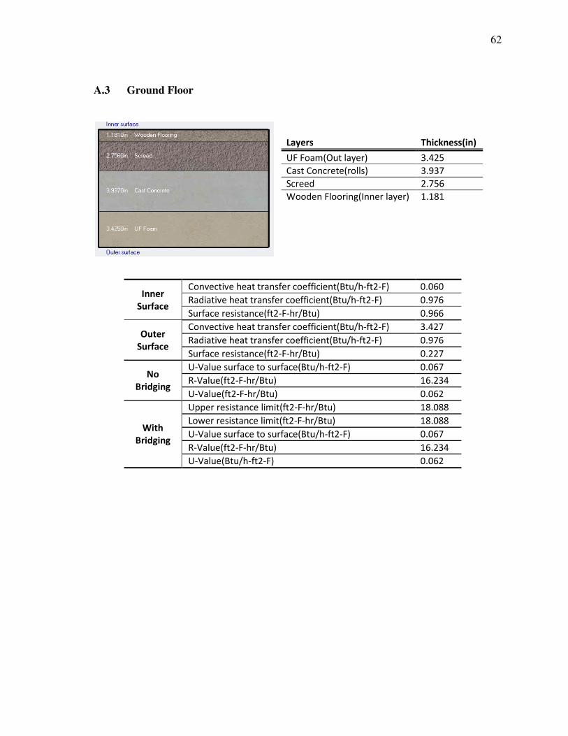
62
A.3 Ground Floor
Inner
Surface
Convective heat transfer coefficient(Btu/h-ft2-F) 0.060
Radiative heat transfer coefficient(Btu/h-ft2-F) 0.976
Surface resistance(ft2-F-hr/Btu) 0.966
Outer
Surface
Convective heat transfer coefficient(Btu/h-ft2-F) 3.427
Radiative heat transfer coefficient(Btu/h-ft2-F) 0.976
Surface resistance(ft2-F-hr/Btu) 0.227
No
Bridging
U-Value surface to surface(Btu/h-ft2-F) 0.067
R-Value(ft2-F-hr/Btu) 16.234
U-Value(ft2-F-hr/Btu) 0.062
With
Bridging
Upper resistance limit(ft2-F-hr/Btu) 18.088
Lower resistance limit(ft2-F-hr/Btu) 18.088
U-Value surface to surface(Btu/h-ft2-F) 0.067
R-Value(ft2-F-hr/Btu) 16.234
U-Value(Btu/h-ft2-F) 0.062
Layers Thickness(in)
UF Foam(Out layer) 3.425
Cast Concrete(rolls) 3.937
Screed 2.756
Wooden Flooring(Inner layer) 1.181
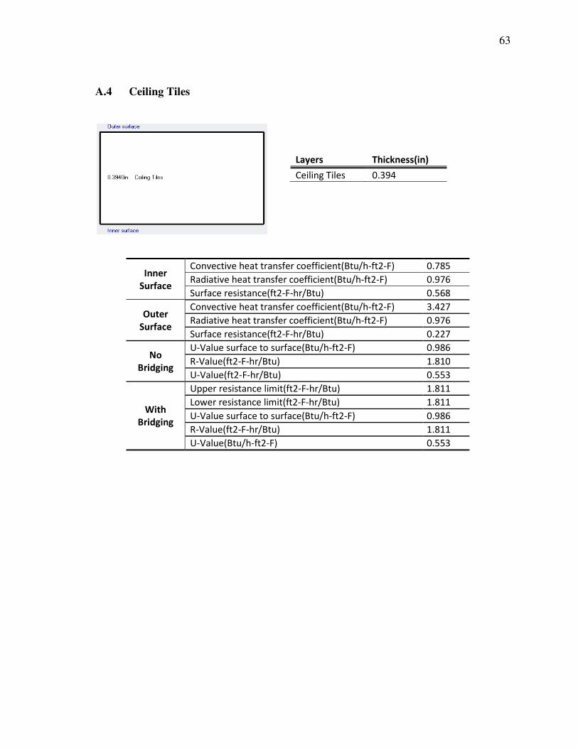
63
A.4 Ceiling Tiles
Inner
Surface
Convective heat transfer coefficient(Btu/h-ft2-F) 0.785
Radiative heat transfer coefficient(Btu/h-ft2-F) 0.976
Surface resistance(ft2-F-hr/Btu) 0.568
Outer
Surface
Convective heat transfer coefficient(Btu/h-ft2-F) 3.427
Radiative heat transfer coefficient(Btu/h-ft2-F) 0.976
Surface resistance(ft2-F-hr/Btu) 0.227
No
Bridging
U-Value surface to surface(Btu/h-ft2-F) 0.986
R-Value(ft2-F-hr/Btu) 1.810
U-Value(ft2-F-hr/Btu) 0.553
With
Bridging
Upper resistance limit(ft2-F-hr/Btu) 1.811
Lower resistance limit(ft2-F-hr/Btu) 1.811
U-Value surface to surface(Btu/h-ft2-F) 0.986
R-Value(ft2-F-hr/Btu) 1.811
U-Value(Btu/h-ft2-F) 0.553
Layers Thickness(in)
Ceiling Tiles 0.394

64
A.5 Internal Walls
Inner
Surface
Convective heat transfer coefficient(Btu/h-ft2-F) 0.379
Radiative heat transfer coefficient(Btu/h-ft2-F) 0.976
Surface resistance(ft2-F-hr/Btu) 0.739
Outer
Surface
Convective heat transfer coefficient(Btu/h-ft2-F) 3.499
Radiative heat transfer coefficient(Btu/h-ft2-F) 0.903
Surface resistance(ft2-F-hr/Btu) 0.227
No
Bridging
U-Value surface to surface(Btu/h-ft2-F) 2.466
R-Value(ft2-F-hr/Btu) 1.372
U-Value(ft2-F-hr/Btu) 0.729
With
Bridging
Upper resistance limit(ft2-F-hr/Btu) 1.372
Lower resistance limit(ft2-F-hr/Btu) 1.372
U-Value surface to surface(Btu/h-ft2-F) 2.466
R-Value(ft2-F-hr/Btu) 1.372
U-Value(Btu/h-ft2-F) 0.729
Layers Thickness(in)
Cast Concrete 3.937
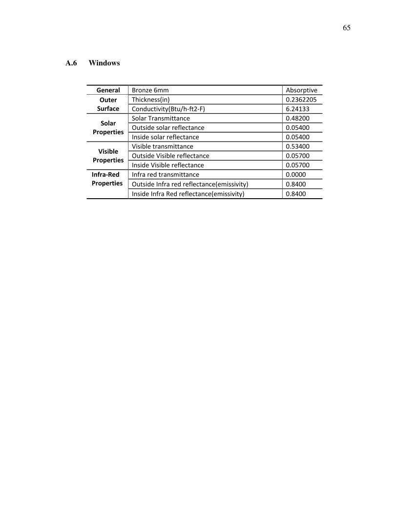
65
A.6 Windows
General Bronze 6mm Absorptive
Outer
Surface
Thickness(in) 0.2362205
Conductivity(Btu/h-ft2-F) 6.24133
Solar
Properties
Solar Transmittance 0.48200
Outside solar reflectance 0.05400
Inside solar reflectance 0.05400
Visible
Properties
Visible transmittance 0.53400
Outside Visible reflectance 0.05700
Inside Visible reflectance 0.05700
Infra-Red
Properties
Infra red transmittance 0.0000
Outside Infra red reflectance(emissivity) 0.8400
Inside Infra Red reflectance(emissivity) 0.8400

66
APPENDIX B
ENERGYPLUS INPUT AND OUTPUT FILES INFORMATION
B.1 HVAC System Diagram of EnergyPlus Input File
B.2 EnergyPlus Standard Output Files
Appendix B has documented EnergyPlus input and output files information of
the case-study building in this research.

67
B.1 HVAC System Diagram of Case-study Building
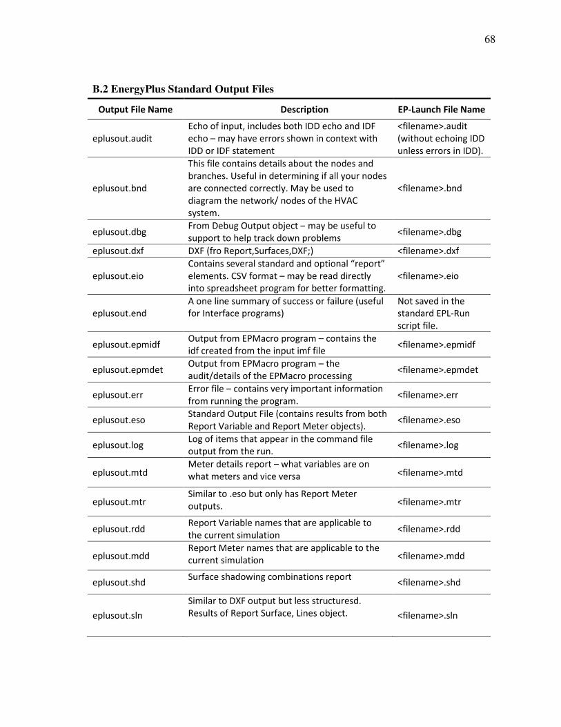
68
B.2 EnergyPlus Standard Output Files
Output File Name Description EP-Launch File Name
eplusout.audit
Echo of input, includes both IDD echo and IDF
echo – may have errors shown in context with
IDD or IDF statement
<filename>.audit
(without echoing IDD
unless errors in IDD).
eplusout.bnd
This file contains details about the nodes and
branches. Useful in determining if all your nodes
are connected correctly. May be used to
diagram the network/ nodes of the HVAC
system.
<filename>.bnd
eplusout.dbg From Debug Output object – may be useful to
support to help track down problems <filename>.dbg
eplusout.dxf DXF (fro Report,Surfaces,DXF;) <filename>.dxf
eplusout.eio
Contains several standard and optional “report”
elements. CSV format – may be read directly
into spreadsheet program for better formatting.
<filename>.eio
eplusout.end
A one line summary of success or failure (useful
for Interface programs)
Not saved in the
standard EPL-Run
script file.
eplusout.epmidf Output from EPMacro program – contains the
idf created from the input imf file <filename>.epmidf
eplusout.epmdet Output from EPMacro program – the
audit/details of the EPMacro processing <filename>.epmdet
eplusout.err Error file – contains very important information
from running the program. <filename>.err
eplusout.eso Standard Output File (contains results from both
Report Variable and Report Meter objects). <filename>.eso
eplusout.log Log of items that appear in the command file
output from the run. <filename>.log
eplusout.mtd Meter details report – what variables are on
what meters and vice versa <filename>.mtd
eplusout.mtr Similar to .eso but only has Report Meter
outputs. <filename>.mtr
eplusout.rdd Report Variable names that are applicable to
the current simulation <filename>.rdd
eplusout.mdd Report Meter names that are applicable to the
current simulation <filename>.mdd
eplusout.shd Surface shadowing combinations report
<filename>.shd
eplusout.sln
Similar to DXF output but less structuresd.
Results of Report Surface, Lines object. <filename>.sln

69
B.2 EnergyPlus Standard Output Files-Continued
Output File Name Description EP-Launch File Name
eplusssz.<ext>
Results from the System Sizing object. This file is
“spreadsheet” ready. Different extensions (csv,
tab, and txt) denote different “separators” in the
file.
<filename>Ssz.<ext>
epluszsz.<ext>
Results from the Zone Sizing object. This file is
“spreadsheet” ready. Different extensions (csv,
tab, and txt) denote different “separators” in the
file.
<filename>Zsz.<ext>
eplusmap.<ext>
Daylighting intensity “map” output. Different
extensions (csv, tab, and txt) denote different
“separators” in the file.
<filename>Map.<ext
>
eplusscreen.csv Window screen transmittance (direct and
reflected) “map” output.
<filename>Screen.cs
v
eplustbl.<ext>
Results of Report Table and Economics requests.
Different extensions (csv, tab, and txt) denote
different “separators” in the file.
<filename>Table.<ex
t>
eplusout.svg
Results from the HVAC-Diagram application. SVG
is a Scalable Vector Graphics file for which
several viewers can be found.
<filename>.svg
eplusout.sci File of cost information <filename>.sci
eplusout.delightin
File produced during Delight simulations –
descriptive of EnergyPlus inputs into Delight
inputs.
<filename>.delightin
eplusout.delightdfd
mp
File produced during DElight simulations – basic
results from DElight simulation.
<filename>.delightdf
dmp
eplusout.delighteld
mp
File produced during DElight simulations –
includes any warning or error messages from
DElight
<filename>.delightel
dmp
eplusout.sparklog File produced during DElight simulations –
timestep results from the simulation <filename>Spark.log
eplusout.wrl
File produced during simulations of SPARK
component models – includes statistics as well as
any warning or error message from the SPARK
link.
<filename>.wrl

70
VITA
Wenshu Fan received her B.E. in mechanical engineering from Tongji
University, Shanghai, China. During the course of her graduate studies at Texas A&M
University, she worked as a research assistant with the Energy Systems Laboratory. Her
area of work and research was related to Continuous Commissioning® and building
energy simulations. Miss Fan graduated with her M.S. at Texas A&M University in
December 2008. Her address is 015 Wisenbaker Engineering Research Center (WERC),
Texas A&M University, College Station, TX, 77843-3581. She can also be reached at
Top Related