


Languages
Pages
Legal


Optimal Reconfiguration for Capacity Expansion of Communication Satellites
Constellations
Afreen SiddiqiJason Mellein
May 3, 2004
16.888 Final Presentation

2
Overview
• Motivation
• Goals
• Optimal Inter-satellite reconfiguration
• Optimal intra-satellite reconfiguration
• Conclusions

3
Motivation
Iridium may have succeeded ifit could ‘reconfigure’ for data as well as voice transmission
Reconfigurable communication satellite systems can mitigate risks and provide greater benefits
Definition: Reconfigurability is a system’s ability to reversibly achieve distinct configurations*, in order to produce new or modified system form and/or function, within an application specific time constant.
*relationships between system elements in the distinct configurations maybe physical, spatial etc.
• Reconfigurable satellite systems can meet new requirements
• Reconfiguration allows capitalization of economic opportunities, or fulfillment of new needs that may arise over time

4
Goals
• Two classes of reconfiguration studied:
• Inter-Satellite reconfiguration– Change in spatial relationships between constellation
satellites– Variation of orbital characteristics (altitude, elevation)
• Intra-Satellite reconfiguration– Change in internal satellites’ sub-systems – Variation of component characteristics to achieve desired
system requirements

5
Inter-Satellite Reconfiguration: Problem Definition
• What is the optimal orbital reconfiguration for an existing satellite constellation to undergo in order to meet a new (and higher) capacity demand?
aa
desiredB
b
b
andhgivenCC
kmhts
ationCostReconfigurJ
ε
ε=
≤≤≤≤
=
(deg)205)(2000400
..min
hb = altitude of B (km)εb = elevation angle of B (deg)Cb = system lifetime capacity (minutes)
N(B)-N(A) satellites on the ground
Constellation A Constellation B
N(B) satellites Earth N(A)
satellites Earth
Orbital transfer
Launch
⎥⎦
⎤⎢⎣
⎡=
b
bhε
x
Design vector:
Formulation:

6
Optimization on two levels
Constellation
Constellation
hbεb
haεa
N,s,p (B)
N,s,p (A) Astrodynamics
parameters
Design vector (x)
∆Vi,j , Ti,j
Optimizer(Auction algorithm)
# of additional sats needed
Launch Fuel
Orbital Assignments
Fuelconsumption
Launch cost/satellite
J = reconfig cost
Cost
Constellation
Link Budget
Optimizer
g(x)= capacity
x*
Function Evaluator
Legend:N: # of satellitesS: # of sats/planesP: # of planes∆V: matrix of ∆VsT: time matrix
Orbit Reconfiguration: SOO - Simulation Model

7
3.1x10114.5x1011System Lifetime Capacity [min]
17921100Voice circuits/sat
250240FDMA channels
10.510.5Bandwidth [MHz]
8.63-Beamwidth [deg]
400400Transmit power [W]
25.5724.3Transmit gain [W]
4.95x10-111010Power flux [Jv]
780780Altitude [km]
6 6# orbital planes
1.62131.6212Frequency [GHz]
6666# of sats
SimulatedActualCharacteristic
Benchmarked against Iridium data
Orbit Reconfiguration: Benchmarking
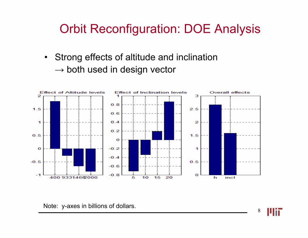
8Note: y-axes in billions of dollars.
• Strong effects of altitude and inclination → both used in design vector
Orbit Reconfiguration: DOE Analysis

9
Orbit ReconfigurationSingle Objective Optimization - I
Full Factorial Computation with ∆h=50[km] and ∆ε=1[deg]
Highly non-linear design space and constraint

10
Algorithm: SQP (fmincon)
Optimizer: MATLAB
x*:J*:
Actual Capacity:
[1066, 5]$587 Million1.008 x 1011[min]
Parameter Values:Cdesired = 1011 minhA = 2000 kmεA = 5 deg
Assumptions:- Polar constellation- Global, single fold coverage
Constellation A:2000 km, 5o
→ 21 satellites3 planes7 sats/plane
CA= 1.5 x 10¹⁰ min
Constellation B:1066 km, 5o
→ 40 satellites5 planes8 sats/plane
CB= 1.008 x 10¹¹ min
Optimal orbital reconfiguration
Sensitivity:⎥⎦
⎤⎢⎣
⎡=⎥
⎦
⎤⎢⎣
⎡∂∂∂∂
=∇0.0899 0.00005-
eJhJ
J
⎥⎦
⎤⎢⎣
⎡=∇=∇
0.7653 0.8569-
. *
*
JJJ x
Orbit Reconfiguration: SO Optimization - II
11
0 10 20 30 40 50 60 70 80 900.5
1
1.5
2
2.5
3
3.5
Iteration Number
Sys
tem
Ene
rgy
SA convergence history
current configurationnew best configuration
10 20 30 40 50 60 70
0.55
0.6
0.65
0.7
0.75
0.8
0.85
0.9
0.95
Iteration Number
Sys
tem
Ene
rgy
SA convergence history
current configurationnew best configuration
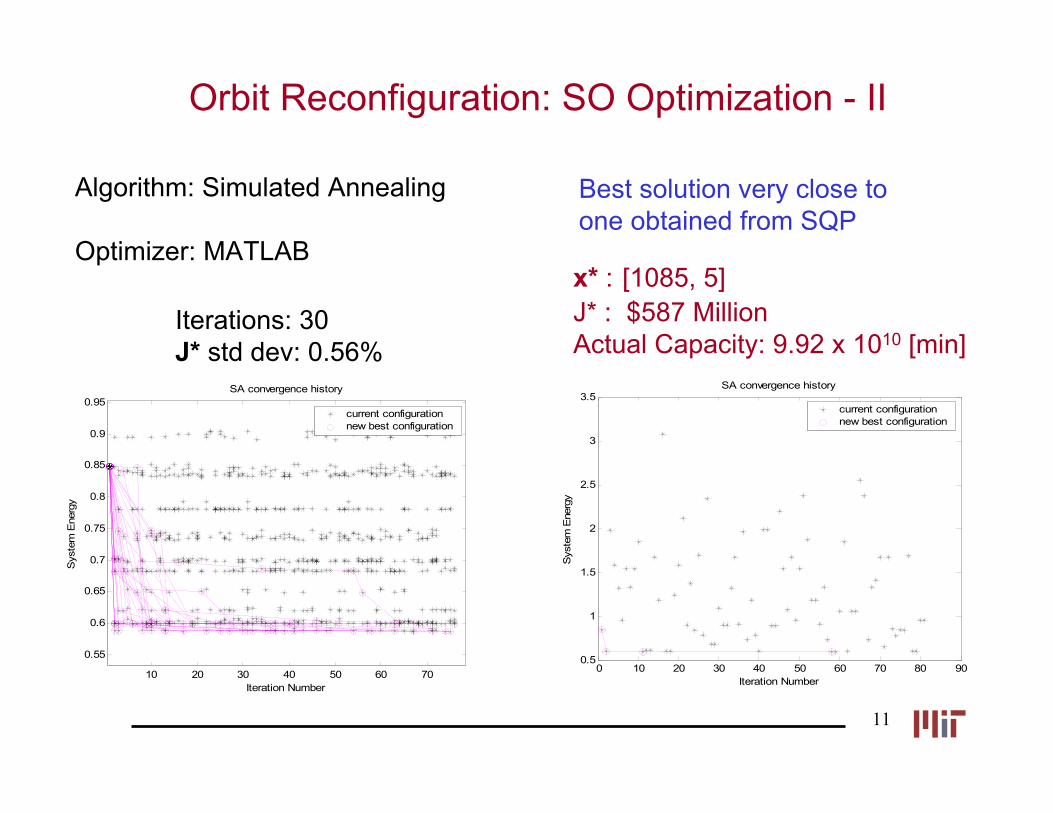
x* : [1085, 5]J* : $587 MillionActual Capacity: 9.92 x 10¹⁰ [min]
Iterations: 30J* std dev: 0.56%
Algorithm: Simulated Annealing
Optimizer: MATLAB
Best solution very close to one obtained from SQP
Orbit Reconfiguration: SO Optimization - II

12
desiredB
B
B
mo
CCand
kmhts
CJCostJ
JJJ
≥
<≤≤≤
==
−−=
(deg)205)(2000400
..
)1(min
2
1
21
ε
λλ
• Capacity Constraint changed from equality to inequality
• Objectives:
J1 = minimize reconfiguration cost
J2 = maximize capacity
• Scaling on the capacity objective due to O(11) difference between J1 and J2:
))((log*)1( 2101 JJJmo λλ −−=
• log10 used due to the variability of J2 over many orders of magnitude in the design space
Orbit Reconfiguration: MO Optimization
13
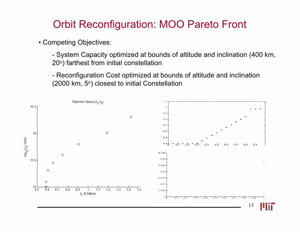
• Competing Objectives:
- System Capacity optimized at bounds of altitude and inclination (400 km, 20o) farthest from initial constellation
- Reconfiguration Cost optimized at bounds of altitude and inclination (2000 km, 5o) closest to initial Constellation
Orbit Reconfiguration: MOO Pareto Front
14
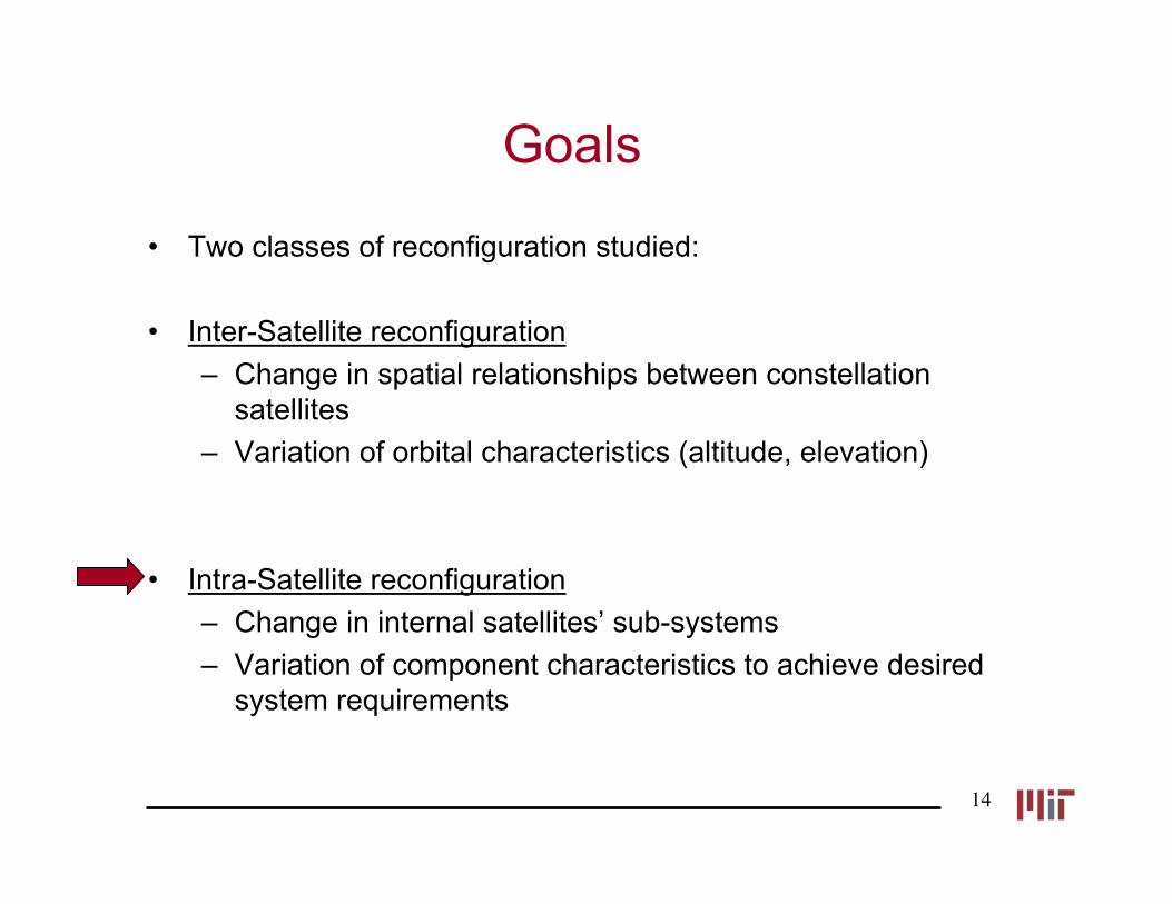
Goals
• Two classes of reconfiguration studied:
• Inter-Satellite reconfiguration– Change in spatial relationships between constellation
satellites– Variation of orbital characteristics (altitude, elevation)
• Intra-Satellite reconfiguration– Change in internal satellites’ sub-systems – Variation of component characteristics to achieve desired
system requirements

15
Intra-Satellite Reconfiguration: Problem Definition
Parameters:h: altitude (km)ε: elevation (deg)xA: satellite component design vector of
constellation A
Design Vector:x: vector of satellite component characteristics
Constellationh, ε
N(# of Sats)
Link BudgetCapacity
Objective Evaluator
x
xA
J
Constants
• What is the optimal reconfiguration the communication components of satellites of an existing constellation should undergo in order to meet a new (and higher) capacity demand?
Simulation Structure

16
Satellite Reconfiguration: DOE Analysis• Several variables affect communication system capacity
– DOE used to determine driving factors
Receiver gain discarded from design vector due to negligible effect on capacity
Chosen design vector:
DA: antenna diameter (m)Pt: transmit power (W)R: single user data rate (kbps)Tsat: satellite lifetime (yrs)Gr: Receiver gain
⎥⎥⎥⎥
⎦
⎤
⎢⎢⎢⎢
⎣
⎡
=
sat
t
a
TRPD
x

17
Satellite Reconfiguration: Problem Formulation
Formulation:
desiredB
sat
t
a
BA
CCand
yearsTkbpsRWPmD
tsJ
=
≤≤≤≤≤≤≤≤
−=
)(155)(104.2
)(80050)(101.0
..min xx
• Two algorithms used
• SQP:– all DVs continuous– repeatable – several ICs used
• Simulated Annealing: – well established heuristic technique – computationally cheaper than GAs

18
Satellite Reconfiguration: Single Objective Optimization
[ ]min107.9075.1
24.552.4
03.4005.2
11
*
*
xCJ
TRPD
B
sat
t
a
B
=
=
⎥⎥⎥⎥
⎦
⎤
⎢⎢⎢⎢
⎣
⎡
=
⎥⎥⎥⎥
⎦
⎤
⎢⎢⎢⎢
⎣
⎡
=x
Parameter Values:Cdesired = 1012 minhA = 780 kmεA = 8.2 degxA =[1.5, 400, 4.8, 5]T
Note: xA had values of Iridium components
CA = 3.1 x 10¹¹ min
Assumptions:- No orbital reconfiguration- On-orbit servicing
Da increased by 1mR decreased by small amountTsat increased by 3 months
Algorithm: SQP (fmincon)
Optimizer: MATLAB
⎥⎥⎥⎥
⎦
⎤
⎢⎢⎢⎢
⎣
⎡
−=∇=∇
09.109.1
019.2
. *
*
JJJ x
⎥⎥⎥⎥
⎦
⎤
⎢⎢⎢⎢
⎣
⎡
−=
⎥⎥⎥⎥
⎦
⎤
⎢⎢⎢⎢
⎣
⎡
∂∂∂∂∂∂∂∂
=∇
22.026.0
094.0
////
sat
t
a
TJRJPJDJ
J
Sensitivity:
Antenna diameteris highest driver

19
Satellite Reconfiguration: SO Optimization -II
x* : [2.5, 400.9, 4.4, 5]J* : 1.48Actual Capacity: 9.86 x 10¹¹ [min]Iterations: 30
J* std dev: 2.42
Algorithm: Simulated Annealing
Optimizer: MATLAB
Best solution close to one obtained from SQP

20
Satellite Reconfiguration: Multi-Objective Optimization
desiredB
sat
t
a
BBA
CCand
yearsTkbpsR
WPmD
tsCJandJ
≥
≤≤≤≤
≤≤≤≤
=−=
)(155)(104
)(1200200)(105.0
..maxmin 21 xx
21 )1( JJz λλ −−=
Competing objectives:- higher capacity →
greater change in component values- lower cost →
smaller change in component values

21
BULLITNUTSBULLITNUTS
High probability that global optimum found
Post Optimality Analysis
• Conditioning and Optimization– Gradient Algorithm started from
various initial conditions – Heuristic Algorithm yielded
feasible design very close to Gradient method results.
• Termination Criteria– Gradient Algorithm converged
consistently– Heuristic Algorithm achieved
Stagnation in Fitness consistently

22
Conclusions
• Orbital and component reconfigurations can be used to increase system capacity if costs can be justified
• Reconfiguration cost vs capacity charts can be used in Constellation Design for Reconfigurability
– Staged deployment followed by reconfiguration
Future Work• Improve:
– capacity calculation– reconfiguration cost estimation– objective for intra-satellite reconfiguration
• Analysis with fixed quality of service, i.e. R not a variable• Explore technologies for intra-satellite reconfiguration

Questions?
24
0
20
40
05001000
150020000
5
10
15
20
25
30
elevation (deg)
# of orbital polar planes on design space
altitude(km)
# of
orb
ital p
olar
pla
nes
010
2030
40
0500
10001500
20000
10
20
30
40
50
elevation (deg)
# of satellites/plane on design space
altitude(km)
# of
sat
ellit
es/p
lane
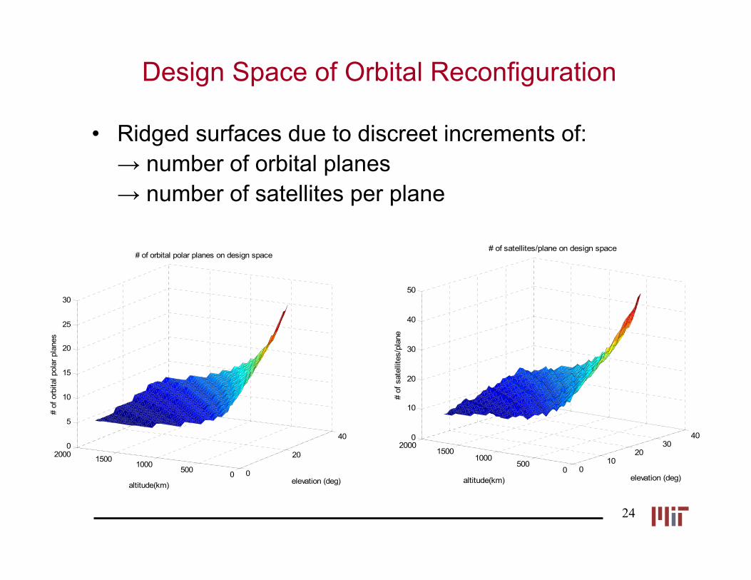
• Ridged surfaces due to discreet increments of: → number of orbital planes→ number of satellites per plane
Design Space of Orbital Reconfiguration

25
Intra-Satellite Reconfiguration Results
• 34 Initial conditions were used• In most cases the same optimal solution was calculated
– Can be assumed that global optimum was found
Top Related