


Languages
Pages
Legal

1
Optimal and Approximate Approaches for Deployment of
Heterogonous Sensing Devices
Rabie Ramadan
Department of Computer
Science and Engineering
Southern Methodist University
Dallas, TX 75275-0122
Hesham El-Rewini
Department of Computer
Science and Engineering
Southern Methodist University
Dallas, TX 75275-0122
Khaled Abdelghany
Department of Environmental
and Civil Engineering
Southern Methodist University
Dallas, TX 75205-0335
Abstract
In this paper, a modeling framework for the problem of deploying a set of heterogeneous
sensors in a field with time-varying differential surveillance requirements is presented. The
problem is formulated as a mixed integer mathematical program with the objective is to
maximize coverage of a given field. Two meta-heuristics are also used to solve this problem. The
first heuristic adopts a Genetic Algorithm (GA) approach while the second heuristic implements
a Simulated Annealing (SA) algorithm. A set of experiments are used to illustrate capabilities of
the developed models and to compare their performance. The experiments investigate the effect
of parameters related to the size of the sensor deployment problem including number of deployed
sensors, size of the monitored field and length of the monitoring horizon. They also examine
several endogenous parameters of the developed GA and SA algorithms.
Keywords: WSN, sensor deployment, Genetic Algorithms and Simulated Annealing
2
1. Introduction
Latest advances in wireless sensing technologies have considerably expanded their
applications including military, homeland and border security, roadway safety and traffic
surveillance, habitat monitoring, and wildlife and environment protection [3,16,17]. In most of
these applications, a network of individual wireless sensors is used to collect state-describing
data from a given field. This data is then transmitted through the network to one or more
predefined sink nodes for processing. Clearly, the performance of a Wireless Sensor Network
(WSN) would largely depend on characteristics and deployment scheme of individual sensors
used to construct this network. Sensors could be characterized by their lifespan, power saving
capabilities, mobile capabilities, reliability, coverage range and communication range. Using
sensors with superior sensing capabilities together with accurate placement of these sensors in
the field’s hot spots would result in more effective surveillance. In this context, WSNs could
generally be classified into a) homogenous vs. heterogeneous and b) ad hoc vs. organized [8, 15].
Homogenous WSNs use identical set of sensors, while heterogeneous WSNs consider sensors
that differ in one or more of the above characteristics. In ad hoc WSNs, sensors are randomly
placed mainly due to limited access to the monitored field. However, in organized WSNs, full
access to the monitored field is granted and hence the exact location of each used sensor over the
monitoring horizon is predefined.
This paper studies organized heterogeneous WSNs. A modeling framework for the
problem of deploying a set of heterogeneous sensors in a field with time-varying differential
surveillance requirements is presented. In this framework, the problem is formulated as a mixed
integer mathematical program with the objective is to maximize coverage of a given field. A set
of constraints are defined for this mathematical program to guarantee that each zone in the
3
monitored field achieves its required surveillance requirements. Constraints are also defined to
ensure that no sensor is used beyond its capacity. The solution of this mathematical program
yields the deployment scheme for each used sensor. Two meta-heuristics are also used to solve
this problem. The first heuristic adopts a Genetic Algorithm (GA) approach while the second
heuristic implements a Simulated Annealing (SA) algorithm. A set of experiments are used to
illustrate capabilities of the developed models and to compare their performance. The
experiments investigate the effect of parameters related to the size of the sensor deployment
problem including number of deployed sensors, size of the monitored field and length of the
monitoring horizon. They also examine endogenous parameters of the developed GA and SA
algorithms.
The contribution of this research work is fourfold. First, the modeling framework
considers the deployed of heterogeneous set of sensors. Most existing sensor deployment
algorithms assume the deployment of identical sensors (see for example, [3,4,6] ). Thus, a more
general framework is needed for large-scale surveillance operations in which multiple sets of
heterogeneous sensors are integrated in one deployment plan. Second, main characteristics of the
sensors such as lifespan, power saving and mobile capabilities and reliability are explicitly
considered. Third, the framework considers monitoring fields with time-varying differential
surveillance requirements. In other words, the framework develops a deployment scheme that is
responsive to the temporal-spatial variation in the criticality of the different zones of the
monitored field. Finally, developed algorithms in this framework generate near-optimal solution
for large-size deployment problems in reasonable running time, which enable the use of these
algorithms in applications that requires real-time sensor deployment.

4
Early contribution to the problem of surveillance device deployment returns to Chvatal,
1975 [21], who introduced the Art Gallery problem. In this problem, the goal is to determine the
minimum number of observers required to secure an art gallery with a non-uniform geometry.
Different versions of this problem have been studied to include mobile guard and guards with
limited visibility (e.g., [11]). Nonetheless, research in the area of sensing devices deployment has
rapidly advanced with the emergence of wireless sensors networks. Most of the research work in
this area has concentrated on studying the optimal formation of a WSN that can be used to
collect data from a given field and to transmit this data to one or more sink points (e.g., [12,14]).
For example, Chakrabarty in [12] proposed a mathematical programming approach for sensor
and target location in distributed sensor networks. The formulation assumes homogenous sensing
devices with perfect accuracy. Isler in [22] proposed concurrent and incremental deployment
methods using sampling theory in which new nodes are deployed based on samples taken from
some other randomly deployed nodes. Liu and Mohapatra [25] proposed an integer linear
program to maximize the overall lifetime of WSNs. A heuristic is proposed where nodes are
forced to send collected data as far as they could and bypass some intermediate nodes to save
their energy. Hu et al. [23] proposed the deployment of superior set of sensors, called
microservers in a hybrid deployment framework. These microservers are used to filter and route
the data in order to reduce the load on other devices. Lee et al. [9] shows mathematically and
using simulation that using sensors with different lifetime might prolong the overall wireless
sensor network’s lifetime.
Deployment of mobile nodes has been described in several contexts. One common
approach assumes availability of a superior leader that guides several mobile sensor nodes to
their deployment positions. Wang et al. [7] proposed an algorithm that uses mobile nodes to

5
cover the blind spots in the monitoring area based on static nodes biding data. In addition, Poduri
et al. [20] introduced an algorithm based on artificial potential fields for self-deployment of
mobile sensor nodes. The algorithm aims to achieve maximum coverage of the monitoring fields.
Furthermore, Howard et al. [2] presented an incremental deployment approach that uses the
information gathered from previously deployed nodes in unknown environment to guide
deploying the rest of the nodes. Issues related to sensors reliability are presented in [18, 27, 28]
considering the deployment of stationary sensing devices with imprecise detection capabilities.
The objective is to maximize the monitoring field coverage for target detection using a set of
devices with probabilistic precessions. In addition, the effect of sensors aging on coverage
performance is studied in [10]. Furthermore, sensor self-scheduling (state-switching) capability
for energy saving purposes is considered in [24, 26]. The goal is to prolong the network life time
through scheduling sensor nodes to be inactive during periods with slow or no activities (e.g.,
off-peak periods).
The paper is organized as follows. The sensor deployment problem is formally defined in
section 2 which also describes the mathematical program developed for the problem. Section 3
presents the GA and SA algorithms used to solve this problem. Experiments that illustrate the
performance of these algorithms are presented in Section 4. Finally, the paper concludes in
section 5.
2. Problem Definition and Formulation
A field )(AG is given. This field is divided into A zones that monitored for a horizon of
length T using a set of surveillance devices S . Each zone Ai is associated with a time-
varying weight function t
iw , where Tt . This weight function defines the importance of the

6
observations (security requirement) in this zone over the periodT . Each device Ss is
characterized by a predefined reliability t
sR that typically declines with the age of the device. In
addition, a surveillance device s is also assumed to have a predefined lifespan (battery life) sL .
Also, each surveillance device is assumed to have limited self-scheduling (state-switching)
capability. Thus, during the monitoring periodT , a surveillance device could be active (on) or
inactive (off). A surveillance device is expected to be active in zone i in time interval t if this
zone’s observation during this time interval is of high value ( t
iw is relatively high). If t
iw is
relatively low, this surveillance device could be turned off to save its power. Thus, it could be
used in other time intervals with high observation weights or in other more important zones. The
maximum number of allowed state switches sP is known for each device s . We define the
variable 1t
siOn if device s is turned to active state by the end of time interval t in zone i , and
0t
siOn otherwise. Similarly, we define the variable 1t
siOff if device s is turned to inactive
state by the end of time interval t in zone i , and 0t
siOff otherwise.
In addition, a surveillance device could be stationary or mobile. If a stationary device is
deployed in a zone, this device is assumed to remain in this zone for the entire lifespan of the
device. On the contrary, a mobile device can cover multiple zones over the surveillance periodT .
All mobile devices are assumed to have no restriction on the start or the end locations of their
deployment tours. We define the binary variable 1tsijm , if device s is moved from zone i to
zone j by the end of time interval t , and 0tsijm otherwise. Each mobile device is assumed to
have a maximum number of allowed moves sM ( 0sM for static devices) during the periodT .
7
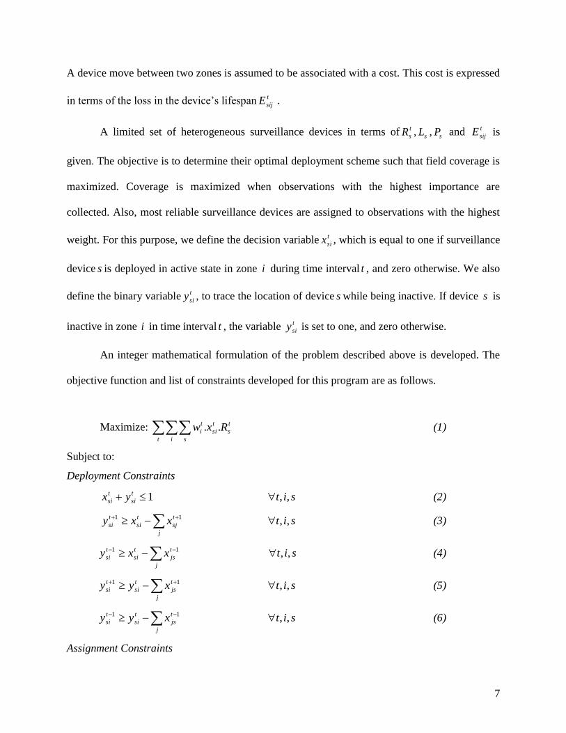
A device move between two zones is assumed to be associated with a cost. This cost is expressed
in terms of the loss in the device’s lifespan t
sijE .
A limited set of heterogeneous surveillance devices in terms of t
sR , sL , sP and t
sijE is
given. The objective is to determine their optimal deployment scheme such that field coverage is
maximized. Coverage is maximized when observations with the highest importance are
collected. Also, most reliable surveillance devices are assigned to observations with the highest
weight. For this purpose, we define the decision variable t
six , which is equal to one if surveillance
device s is deployed in active state in zone i during time interval t , and zero otherwise. We also
define the binary variable t
siy , to trace the location of device s while being inactive. If device s is
inactive in zone i in time interval t , the variable t
siy is set to one, and zero otherwise.
An integer mathematical formulation of the problem described above is developed. The
objective function and list of constraints developed for this program are as follows.
Maximize: t
s
t
si
t i s
t
i Rxw .. (1)
Subject to:
Deployment Constraints
1 t
si
t
si yx sit ,, (2)
j
t
sj
t
si
t
si xxy 11 sit ,, (3)
j
t
js
t
si
t
si xxy 11 sit ,, (4)
j
t
js
t
si
t
si xyy 11 sit ,, (5)
j
t
js
t
si
t
si xyy 11 sit ,, (6)
Assignment Constraints

8
i
t
si
t
si yx 1 st, (7)
s
t
six 1 it, (8)
Mobility Constraints
111 t
si
t
si
t
sj
t
sj
t
sij yxyxm sjijit ,,,, (9)
11 t
sj
t
sj
t
sij yxm sjit ,,, (10)
t
si
t
si
t
sij yxm sjit ,,, (11)
i
s
j t
t
sij Mm s (12)
State Switching Constraints
11 t
si
t
si
t
si yxOn sit ,, (13)
1 t
si
t
si xOn sit ,, (14)
t
si
t
si yOn sit ,, (15)
11 t
si
t
si
t
si xyOff sit ,, (16)
1 t
si
t
si yOff sit ,, (17)
t
si
t
si xOff sit ,, (18)
t i
s
t
si
t
si POffOn s (19)
Lifespan Constraints
s
i j t
t
sij
t
sij
t i
t
si LmEx s (20)
Binary Constraints
},,,,{ t
si
t
si
t
sij
t
si
t
si OffOnmyx = 1 or 0 sit ,, (21)
As shown in (1), the objective function maximizes the field coverage which is described
as the sum over all time intervals, zones and surveillance devices of the products of the
observation weight t
iw , the decision variable t
six ( 1t
six , if device s exists in active state in zone i
in time interval t ) and the reliability of the used device t
sR .

9
Constraints in (2) ensure that a surveillance device is either active or inactive during any
time interval. Constraints in (3) to (6) determine the value of the binary variable t
siy based on the
value of t
six . If a surveillance device is set to be active in zone i during time interval t , and this
device is not used in any zone during the next (previous) time interval, this device is assumed to
be inactive and to stay in this zone during the next (previous) time interval. Similarly, if a device
is set to be inactive in zone i during time interval t , and this device is not used in any zone during
the next (previous) time interval, this device is assumed to remain inactive in the same zone
during the next (previous) time interval. Constraints in (7) ensure that each zone is covered by at
most one device in any time interval. Also, at each time interval, a surveillance device is
covering at most one zone, which is guaranteed in constraints (8).
Constraints in (9) to (11) determine if surveillance device s is moved from zone i to zone
j at the end of interval t . They compare zones where surveillance device s is deployed during
time intervals t and 1t . The binary variable t
sijm is set to one if they are different. Constraints in
(12) ensures that number of moves made by a device is less than or equal to maximum number of
moves allowed for this device.
The state-switches of a surveillance device from active state to inactive state and vice
versa are determined in constraints (13) to (18). The binary variables t
six and t
siy are examined
for each surveillance device while being deployed in every zone. If both variables are equal to
one in two successive time intervals, it indicates that the device’s state is altered. The total
number of state switches for each surveillance device is computed and compared to the
maximum number of switches allowed for each device as given in constraints (19). Constraints
in (20) ensure that each surveillance device is not utilized beyond its lifespan. The consumption
of a device’s lifespan is computed as the sum over all intervals in which the device is active plus

10
the loss in the device lifespan associated with its moves along the different zones. Finally, the
integrality of all binary variables is preserved in constraints (21).
3. Meta Heuristic Approximate Approaches
Due to the intractability of this problem, seeking optimal deployment schemes for large-
scale problems might be impractical. In this section, we present two approximate meta-heuristics
to solve large-scale sensor deployment problems. These heuristics adopt Genetic Algorithm and
Simulated Annealing approaches, respectively. Details on modeling and implementation issues
of these two algorithms are provided in the following subsections.
3.1 The Genetic Algorithm Approach
GA is a machine-learning model, which adopts its behavior from the processes of
evolution in nature. This is done by the creation of a population of individuals represented by
chromosomes. Individuals in the population continuously go through a process of evolution to
increase their fitness and adaptiveness to their environments. The evolution is made up through
exchanging characteristics with other elements of the population (crossover) or through self-
changes in the element (mutation). New generations appear from cloning of the current
population, in proportion to their fitness. The fitness is a single objective (evaluation) function of
the chromosome that returns a numerical value to differentiate between good and bad ones.
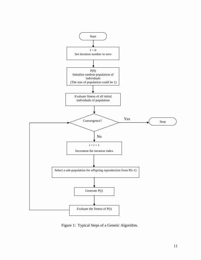
Figure 1 gives a flow chart of a typical GA. The details of the algorithm and its advanced
features can be found in [1,5,13]. A typical GA starts by generating a set of initial chromosomes
(initial population). This is usually done following a random procedure. Then, each of these
chromosomes is evaluated through objective (evaluation) function to obtain their fitness. While a
satisfactory chromosome is not obtained, the algorithm selects from the previous population a set
11
Figure 1: Typical Steps of a Genetic Algorithm.
Start
I = 0
Set iteration number to zero
P(0)
Initialize random population of
individuals
(The size of population could be 1)
Evaluate fitness of all initial
individuals of population
Select a sub-population for offspring reproduction from P(i-1)
Generate P(i)
i = i + 1
Increment the iteration index
Convergence?
No
Evaluate the fitness of P(i)
Yes Stop

12
of chromosomes to be defined as parents (different selection criteria are possible and well
defined in the GA literature). These parents are selected such that they have higher fitness
compared to other chromosomes in the population. Then, these parents are used to generate a
new population (set of chromosomes), also known as children. These children are generated by
crossover methods in which genes of two parents are swapped such that each two parents
generate two children. Children can also be generated by mutation methods in which a single
parent is perturbed to generate a new child. The methods of crossover and mutation are well
defined in the literature [1].
Applying GA to the sensor deployment problem, chromosomes are designed to describe a
feasible deployment plan for the set of available sensors. The length of each chromosome
(number of genes) is taken to be equal to |A| * |T| * |S|, where |A|, |T|, |S| are number of zones,
number of intervals in the monitoring horizon and number of sensors, respectively. If sensor
Ss is deployed in zone Az in time interval Tt , the gene represents s, z and t is set to one
and zero otherwise. Figure 2 illustrates the structure of a chromosome used to represent the
deployment of two sensors (s1 and s2) in a field of four zones (z1, z2, and z3) which is monitored
for two time intervals (t1 and t2). As shown in the Figure, s1 is used for the two time intervals
and is moved once to cover z3 at t1 and z1 at t2. Thus, s1 does not exercise the state-switching
capability. Sensor s2 is used only for the first time interval (t1); then turned off at time t2.
t1 t2
z1 z2 z3 z1 z2 z3 z1 z2 z3 z1 z2 z3
0 0 1 0 1 0 1 0 0 0 0 0
s1 s2 s1 s2
Figure 2: Example of a Chromosome for the Sensor Deployment Problem.
13
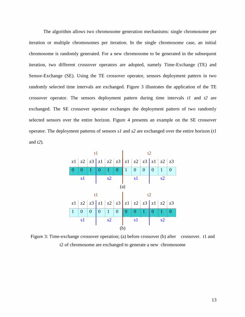
The algorithm allows two chromosome generation mechanisms: single chromosome per
iteration or multiple chromosomes per iteration. In the single chromosome case, an initial
chromosome is randomly generated. For a new chromosome to be generated in the subsequent
iteration, two different crossover operators are adopted, namely Time-Exchange (TE) and
Sensor-Exchange (SE). Using the TE crossover operator, sensors deployment pattern in two
randomly selected time intervals are exchanged. Figure 3 illustrates the application of the TE
crossover operator. The sensors deployment pattern during time intervals t1 and t2 are
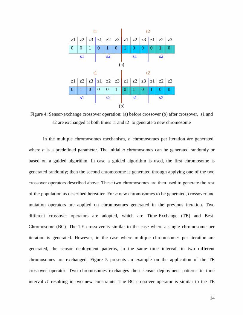
exchanged. The SE crossover operator exchanges the deployment pattern of two randomly
selected sensors over the entire horizon. Figure 4 presents an example on the SE crossover
operator. The deployment patterns of sensors s1 and s2 are exchanged over the entire horizon (t1
and t2).
t1 t2
z1 z2 z3 z1 z2 z3 z1 z2 z3 z1 z2 z3
0 0 1 0 1 0 1 0 0 0 1 0
s1 s2 s1 s2
(a)
t1 t2
z1 z2 z3 z1 z2 z3 z1 z2 z3 z1 z2 z3
1 0 0 0 1 0 0 0 1 0 1 0
s1 s2 s1 s2
(b)
Figure 3: Time-exchange crossover operation; (a) before crossover (b) after crossover. t1 and
t2 of chromosome are exchanged to generate a new chromosome
14
t1 t2
z1 z2 z3 z1 z2 z3 z1 z2 z3 z1 z2 z3
0 0 1 0 1 0 1 0 0 0 1 0
s1 s2 s1 s2
(a)
t1 t2
z1 z2 z3 z1 z2 z3 z1 z2 z3 z1 z2 z3
0 1 0 0 0 1 0 1 0 1 0 0
s1 s2 s1 s2
(b)
Figure 4: Sensor-exchange crossover operation; (a) before crossover (b) after crossover. s1 and
s2 are exchanged at both times t1 and t2 to generate a new chromosome
In the multiple chromosomes mechanism, n chromosomes per iteration are generated,
where n is a predefined parameter. The initial n chromosomes can be generated randomly or
based on a guided algorithm. In case a guided algorithm is used, the first chromosome is
generated randomly; then the second chromosome is generated through applying one of the two
crossover operators described above. These two chromosomes are then used to generate the rest
of the population as described hereafter. For n new chromosomes to be generated, crossover and
mutation operators are applied on chromosomes generated in the previous iteration. Two
different crossover operators are adopted, which are Time-Exchange (TE) and Best-
Chromosome (BC). The TE crossover is similar to the case where a single chromosome per
iteration is generated. However, in the case where multiple chromosomes per iteration are
generated, the sensor deployment patterns, in the same time interval, in two different
chromosomes are exchanged. Figure 5 presents an example on the application of the TE
crossover operator. Two chromosomes exchanges their sensor deployment patterns in time
interval t1 resulting in two new constraints. The BC crossover operator is similar to the TE

15
operator with the exception that only the two fittest chromosomes are used as parents for all new
chromosomes. Following the crossover operations, the mutation operation is used to prevent the
search from getting trapped in the local minima and also to prevent chromosomes repetition. In
the mutation step, some of the generated chromosomes genes are randomly altered (from zero to
one or vise versa). Thus, the search is directed to a new area in the search space. Figure 6 depicts
an example of the mutation step for a single chromosome.
. t1 t2
z1 z2 z3 z1 z2 z3 z1 z2 z3 z1 z2 z3
0 0 1 0 1 0 1 0 0 0 1 0
s1 s2 s1 s2
t1 t2
z1 z2 z3 z1 z2 z3 z1 z2 z3 z1 z2 z3
0 1 0 0 0 1 0 1 0 1 0 0
s1 s2 s1 s2
(a)
t1 t2
z1 z2 z3 z1 z2 z3 z1 z2 z3 z1 z2 z3
0 1 0 0 0 1 1 0 0 0 1 0
s1 s2 s1 s2
t1 t2
z1 z2 z3 z1 z2 z3 z1 z2 z3 z1 z2 z3
0 0 1 0 1 0 0 1 0 1 0 0
s1 s2 s1 s2
(b)
Figure 5: Time-exchange crossover operation between two chromosomes; (a) before
crossover (b) after crossover. t1 in both chromosomes are exchanged to generate two new
chromosomes

16
t1 t2
z1 z2 Z3 z1 z2 z3 z1 z2 z3 z1 z2 z3
0 0 0 0 1 0 1 0 0 0 0 0
s1 s2 s1 s2
t1 t2
z1 z2 z3 z1 z2 z3 z1 z2 z3 z1 z2 z3
1 0 0 0 0 1 0 1 0 0 1 0
s1 s2 s1 s2
Figure 6: Mutation operation; s1 at t1 and s2 at t2 are muted to be used on z1 and z2
respectively
Crossover and mutation operations could result in unfeasible chromosomes as some
sensors might exceed their capabilities (e.g., lifespan, maximum number of moves, and
maximum number of allowed switches). As such, a feasibility check routine is applied for each
newly generated chromosome to ensure that all chromosomes in the population are representing
feasible deployment patterns.
The fitness of each generated chromosomes is measured using the fitness function given
below. One should notice the similarity between this fitness function and the objective function
of the mathematical program in §2.
t
s
t i s
t
i RwxF .)( , where x is the chromosome identifier. (22)
Given the fitness value for each new chromosome, chromosomes are added as part of the
current population only if they outperform the current available solution. The algorithm stopping
criteria could be based on a fixed number of iterations or a given number of iterations in which
the solution does not improve.

17
3.2 The Simulated Annealing Approach
Simulated Annealing (SA) is a randomized search technique for highly nonlinear problems
[19]. In its search process, the algorithm is similar to using a bouncing ball that can bounce over
mountain from valley to valley based on the ball’s temperature until the highest tip is found. The
algorithm starts by generating an initial feasible solution and computing its performance. This
solution is stored as the best solution obtained so far. Neighborhood of this solution is searched
and a new solution is generated. If the new solution’s performance is greater than the highest
gain found so far (uphill move), the new solution is accepted and saved. If the gain of the new
solution is less than the upper bound performance found so far, still accept this new inferior
solution but with some probability (downhill move). The probability of accepting inferior
solutions is reduced after each iteration (increase of the ball temperature). The process continues
until no better solution is found indicating that the maximum possible temperature is achieved. A
formal description of the SA algorithm can be described using the following main steps:
Define,
X0 = initial solution, and the best solution so far,
Xk = current solution,
N(Xk) = neighborhood of the current solution,
G(Xk) = performance of the current solution,
X̂ = variable to keep the best solution
k = current temperature,
f = final temperature (highest temperature value),
= heating rate for temperature schedule,
P(Xk+1, Xk) = probability of acceptance a new solution (Xk+1) given that the solution is (Xk). This
probability is calculated as follows:
P(Xk+1, Xk) = kf
kk XGXG
e
)()( 1
.
18
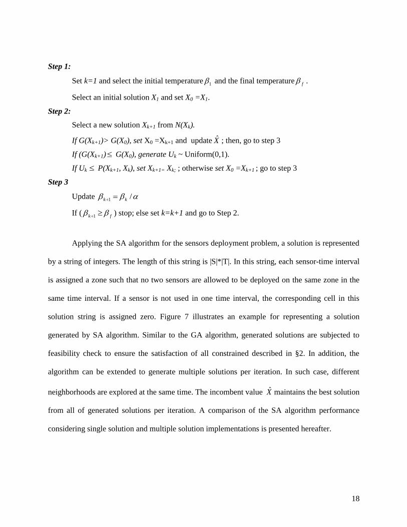
Step 1:
Set k=1 and select the initial temperature 1 and the final temperature f .
Select an initial solution X1 and set X0 =X1.
Step 2:
Select a new solution Xk+1 from N(Xk).
If G(Xk+1)> G(X0), set X0 =Xk+1 and update X̂ ; then, go to step 3
If (G(Xk+1) G(X0), generate Uk ~ Uniform(0,1).
If Uk P(Xk+1, Xk), set Xk+1= Xk; ; otherwise set X0 =Xk+1 ; go to step 3
Step 3
Update /1 kk
If ( fk 1 ) stop; else set k=k+1 and go to Step 2.
Applying the SA algorithm for the sensors deployment problem, a solution is represented
by a string of integers. The length of this string is |S|*|T|. In this string, each sensor-time interval
is assigned a zone such that no two sensors are allowed to be deployed on the same zone in the
same time interval. If a sensor is not used in one time interval, the corresponding cell in this
solution string is assigned zero. Figure 7 illustrates an example for representing a solution
generated by SA algorithm. Similar to the GA algorithm, generated solutions are subjected to
feasibility check to ensure the satisfaction of all constrained described in §2. In addition, the
algorithm can be extended to generate multiple solutions per iteration. In such case, different
neighborhoods are explored at the same time. The incombent value X̂ maintains the best solution
from all of generated solutions per iteration. A comparison of the SA algorithm performance
considering single solution and multiple solution implementations is presented hereafter.

19
t1 t2 t3
z1 0 z4 z2 z4 z3 0 z4 z2
s1 s2 s3 s1 s2 s3 s1 s2 s3
Figure 7: example on the simulated annealing solution in which 4 zones are monitored by 3
sensors for 3 time unites
4. Experimental Results
4.1 GA and SA Benchmarking and Comparison
The mathematical program described in §2 is used to provide an optimal solution for the
sensor deployment problem. The commercial optimization package CPLEX 8.0 running on a 2.4
GHz machine with 2 GB memory is used to generate the optimal solution for different problem
settings. This optimal solution is used to benchmark the performance of solutions obtained by the
GA and SA algorithms. Three different sets of experiments are conducted. These experiments
study the effect of increasing number of zones, number of sensors and time horizon on the
running time required to generate the optimal solution, respectively. In all experiments, the
time-varying observations on the different zones were generated randomly following a uniform
distribution U(0,200). In addition, a heterogeneous set of sensors is assumed. The sensors’
operational characteristics sL , sM and sP are generated randomly as function of the length of
monitored horizon. For example, if the monitoring horizon is T intervals, the sensor lifespan,
maximum allowed number of moves, and maximum allowed number of state switching are
generated randomly using the uniform distribution U(1,T ). All sensors are assumed to be 100%
reliable.
As illustrated in Table 1, the running time required to generate the optimal solution
increases exponentially with the increase in the size of the problem. For instance, a running time
20
of 1542.4 seconds is recorded for a problem of 10 zones, five sensors and a horizon of 12
intervals. This running time jumps to 59031.1 seconds when number of zones is increased to 30.
Problem settings with dimensions beyond the ones presented in the table could not be generated
using the machine mentioned above. The results indicate that both GA and SA algorithms
provide high quality solutions. In the experiment with lowest performance (experiment 5 using
the SA), 85% of the optimal objective function value is obtained. Furthermore, up to 99% of the
corresponding optimal performance is recorded when the GA algorithm is used in experiments 1
and 9. The running time of both algorithms is noticeably small compared to that of the optimal
solution. For example, in experiment 1, the running times of the GA and SA algorithms are
observed to be 0.05% and 0.06% of the optimal solution’s running time, respectively.
Table 1: Performance of the GA and SA algorithms compared to the optimal solution.
Exp No.
No. of
zones
No. of
sensors
Horizon
Optimal
Solution
Running Time
(Sec)
GA
Single Solution per iteration
Time Exchange crossover
SA
Single Solution per iteration
Objective
Function %
Running
Time %
Objective
Function %
Running
Time %
1 10 5 12 1542.4 99 0.06 97 0.05
2 20 5 12 18012.4 91 0.007 92 0.06
3 25 5 12 29057.9 91 0.009 87 0.008
4 30 5 12 59031.1 91 0.005 80 0.005
5 20 3 12 1500.1 89 0.005 85 0.06
6 20 5 12 18012.5 91 0.007 92 0.06
7 20 10 12 1628723 97 0.0003 97 0.0002
8 20 5 3 100.2 94 0.7 93 0..5
9 20 5 6 1010.3 99 0.1 98 0.1
10 20 5 12 18012.4 91 0.007 92 0.06
In most of these experiments, the GA outperforms the SA in terms of objective function.
On the other hand, the SA seems to converge faster than GA algorithm. These results are
confirmed in Figure 8 which illustrates the comparison results of the GA and SA algorithms
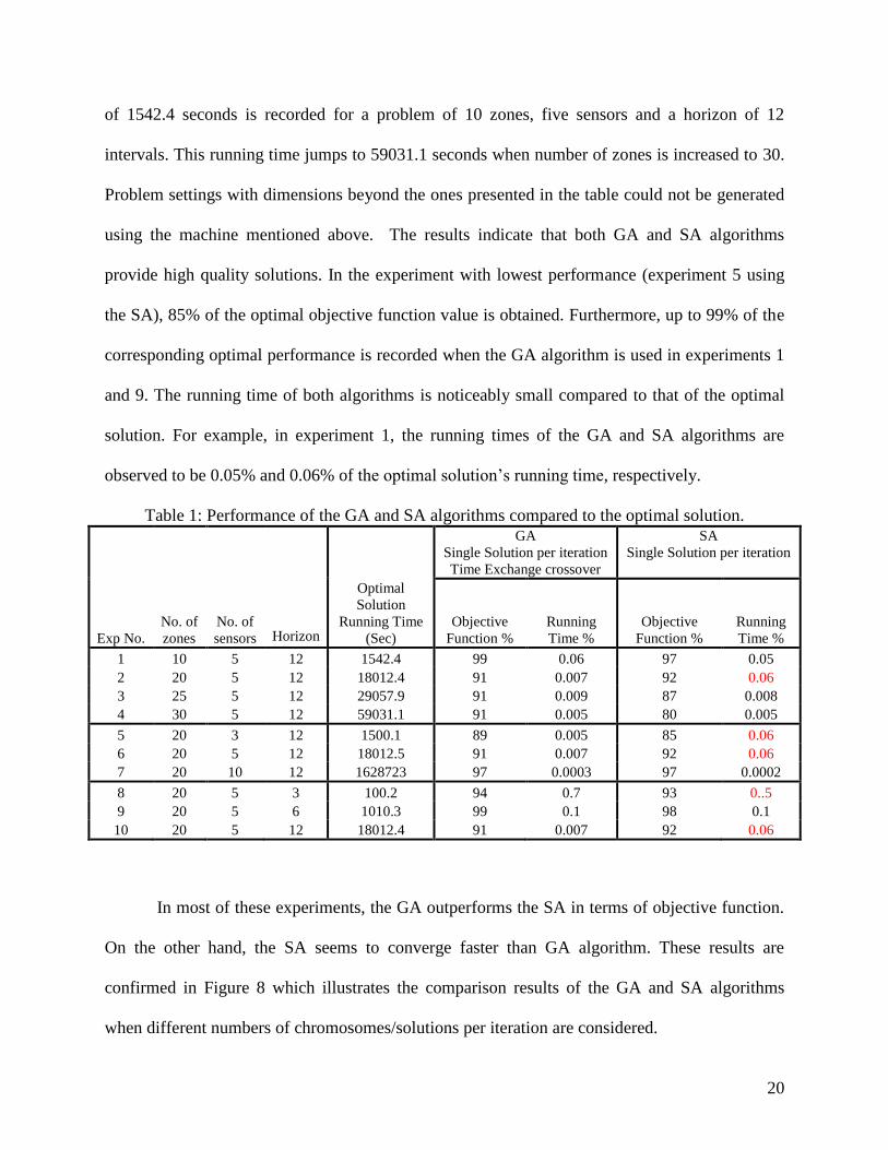
when different numbers of chromosomes/solutions per iteration are considered.
21
0
2000
4000
6000
8000
1 5 10 20 30 40 50
Number of Chromosomes/Solutions
Obje
ctiv
e P
erf
orm
ance GA SA
(a)
0
2000
4000
6000
8000
10000
12000
1 5 10 20 30 40 50
Number of Chromosomes/Solutions
Ela
pse
d T
ime
(s) GA SA
(b)
Figure 8: (a) A comparison between genetic and simulated annealing algorithms with different
chromosomes/solutions per iteration, (b) The running time of genetic and simulated annealing
algorithms
The number of chromosomes/solutions per iteration is set to range from 1 to 50. The
Figure presents the comparison in terms of objective performance and running time. In this set of
experiments, 300 zones are monitored for 12 time intervals using 200 sensors. Zones weights and
sensors capabilities are generated randomly as mentioned above. As shown in Figure 8a, the
genetic algorithms outperform the simulated annealing algorithm in terms of the objective
function. On average, the recorded objective performance for the SA algorithm is almost 96% of
the genetic algorithm performance. However, the SA running time is less than that of the GA
running time by 9%. This set of experiments also illustrates the impact of the number of
chromosomes/solutions per iteration on the solution performance. In general, increasing the
number of solutions per iteration resulted in convergence at a better objective function for both
algorithms. This is achieved on the expense of the running time, however. For example, the
objective performance of a single chromosome/solution is almost 70% of that when 50
chromosome/solutions per iteration are generated. The required time for a single

22
chromosome/solution is approximately 0.02% of the 50 chromosomes/solutions per iteration
case.
4.2 GA Related Results
In this section, we present results related to the GA algorithm. First, the algorithm
convergence pattern is presented for the cases of single and multiple chromosomes. Then, the
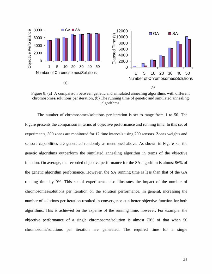
effect of crossover and mutation strategies on the solution quality is illustrated. Figure 9 shows
the objective performance and corresponding running time for a deployment problem with 100
zones, 50 sensors and 12 time intervals. The value of the objective performance and the
corresponding cumulative running time are recorded after every iteration. SE crossover operator
and 100% mutation are used in these experiments. As shown in Figure 9a, generating 10
chromosomes per iteration results in convergence at higher objective using less number of
iterations. For instance, in the multiple chromosomes case, an objective of 24841 units is
recorded at iteration 64. This value is achieved at iteration 156 in the single chromosome case.
On the other hand, the running time of multiple chromosomes are higher than the time recorded
for the single chromosome case. As shown in the Figure 9b, the running time in the single
chromosome implementation is almost 60% of that recorded in the multiple chromosomes
implementation.
23
0
5000
10000
15000
20000
25000
30000
35000
0 50 100 150 200 250 300
Number of iterations
Ob
jective
pe
rfo
rma
nce
Single chromosme
Multiple chromosmes
(a)
0
5000
10000
15000
0 50 100 150 200 250
Number of iterations
Ru
nn
ing
tim
e (
s)
Single chromosome
Multiple chromosomes
(b)
Figure 9: GA performance progress with number of iterations (a) Objective performance (b)
Running time
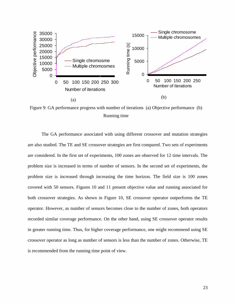
The GA performance associated with using different crossover and mutation strategies
are also studied. The TE and SE crossover strategies are first compared. Two sets of experiments
are considered. In the first set of experiments, 100 zones are observed for 12 time intervals. The
problem size is increased in terms of number of sensors. In the second set of experiments, the
problem size is increased through increasing the time horizon. The field size is 100 zones
covered with 50 sensors. Figures 10 and 11 present objective value and running associated for
both crossover strategies. As shown in Figure 10, SE crossover operator outperforms the TE
operator. However, as number of sensors becomes close to the number of zones, both operators
recorded similar coverage performance. On the other hand, using SE crossover operator results
in greater running time. Thus, for higher coverage performance, one might recommend using SE
crossover operator as long as number of sensors is less than the number of zones. Otherwise, TE
is recommended from the running time point of view.
24
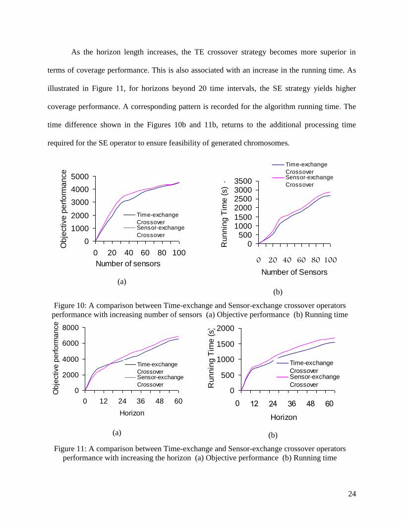
As the horizon length increases, the TE crossover strategy becomes more superior in
terms of coverage performance. This is also associated with an increase in the running time. As
illustrated in Figure 11, for horizons beyond 20 time intervals, the SE strategy yields higher
coverage performance. A corresponding pattern is recorded for the algorithm running time. The
time difference shown in the Figures 10b and 11b, returns to the additional processing time
required for the SE operator to ensure feasibility of generated chromosomes.
0
1000
2000
3000
4000
5000
0 20 40 60 80 100
Number of sensors
Ob
jective
pe
rfo
rma
nce
Time-exchange
CrossoverSensor-exchange
Crossover
(a)
0500
10001500
2000250030003500
0 20 40 60 80 100Number of Sensors
Ru
nn
ing
Tim
e (
s)
-
Time-exchange
CrossoverSensor-exchange
Crossover
(b)
Figure 10: A comparison between Time-exchange and Sensor-exchange crossover operators
performance with increasing number of sensors (a) Objective performance (b) Running time
0
2000
4000
6000
8000
0 12 24 36 48 60
Horizon
Ob
jective
pe
rfo
rma
nce
Time-exchange
CrossoverSensor-exchange
Crossover
(a)
0
500
1000
1500
2000
0 12 24 36 48 60
Horizon
Ru
nn
ing
Tim
e (
s)
Time-exchange
CrossoverSensor-exchange
Crossover
(b)
Figure 11: A comparison between Time-exchange and Sensor-exchange crossover operators
performance with increasing the horizon (a) Objective performance (b) Running time

25
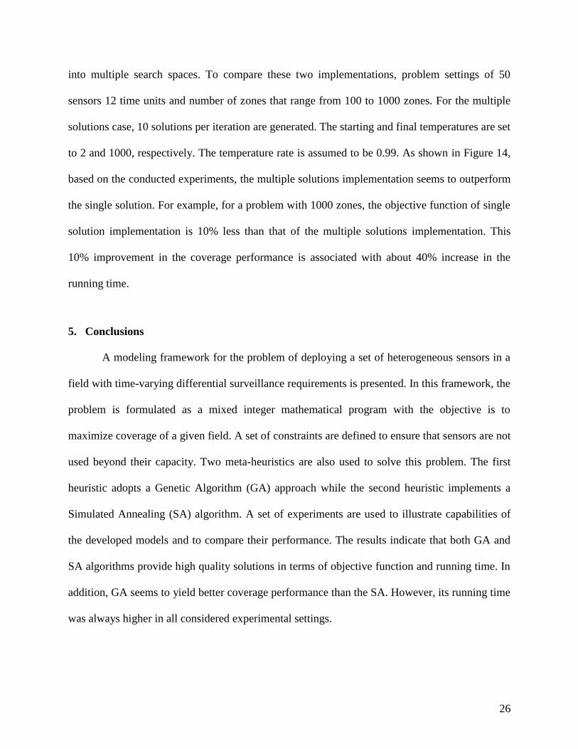
As mentioned above, mutation in GA plays an important role in directing the solution
towards different search spaces. Figure 12 illustrates the effect of using different mutation
percentage on the average objective performance. Mutation percentage is measured as the ratio
between number of altered genes and total chromosome length. A field of 100 zones is
monitored for 12 units of time using 50 sensors. Ten chromosomes per iteration and TE
crossover operator are used throughout these experiments. The mutation percentage ranges from
0% to 100%. The results show that as the mutation percentage increases, the objective
performance increases. For instance, at 20% mutation rate, an objective of 9376 units is
recorded. The objective increased to 10389 units at 100% mutation rate.
4.3 SA Related Results
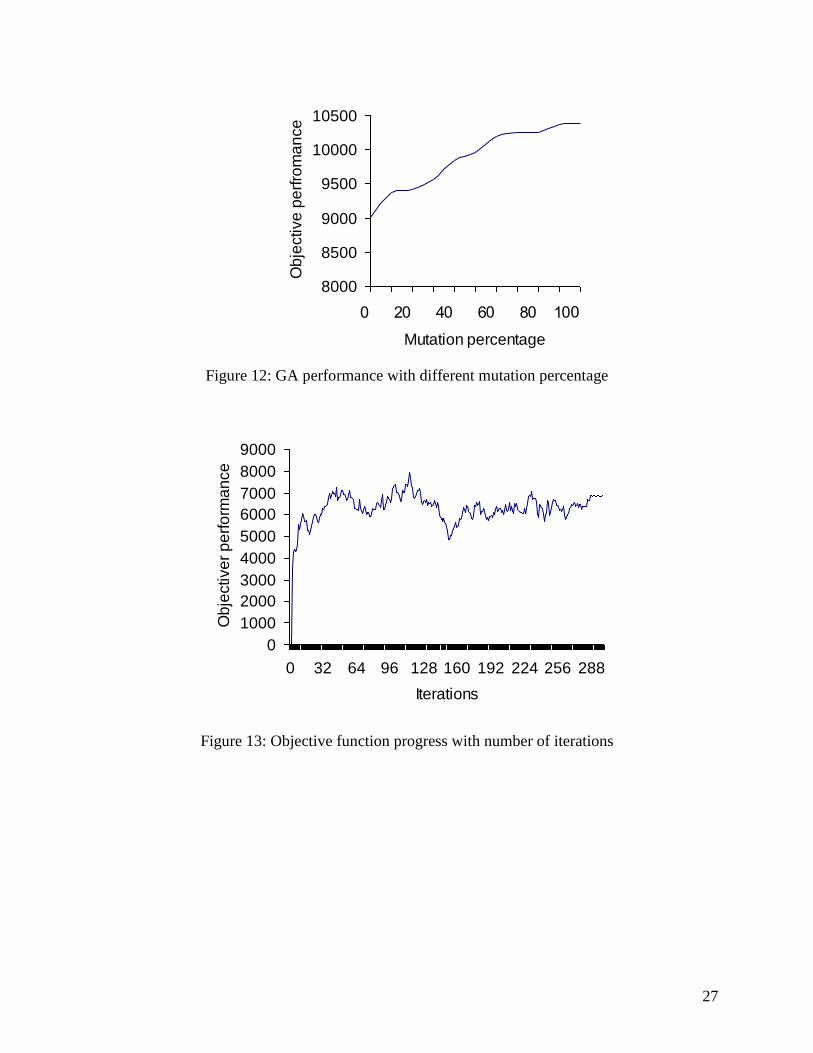
The SA objective function convergence pattern is presented in this section. For this
purpose, the SA algorithm is applied for a problem of 100 zones, 12 time units and 50 sensors.
The heating rate is selected to be 0.99 and a sample of 300 iterations is recorded. The starting
temperature is assumed to be 2 temperature units and the final temperature is set to 50. As shown
in Figure 13, the algorithm starts by pivoting at solutions with low objective values since the
acceptance probability of a new solution is initially high. This may lead the algorithm to fall in a
local minimum such as the fall occurred at iteration 154. Also, the incumbent value ^
X maintains
the highest objective value which is 7939 reached at iteration 114. As the temperature increases,
the acceptance probability is decreased, and the chance of pivoting at low performance solutions
decreases. This pattern is clearly showed starting at iteration 200.
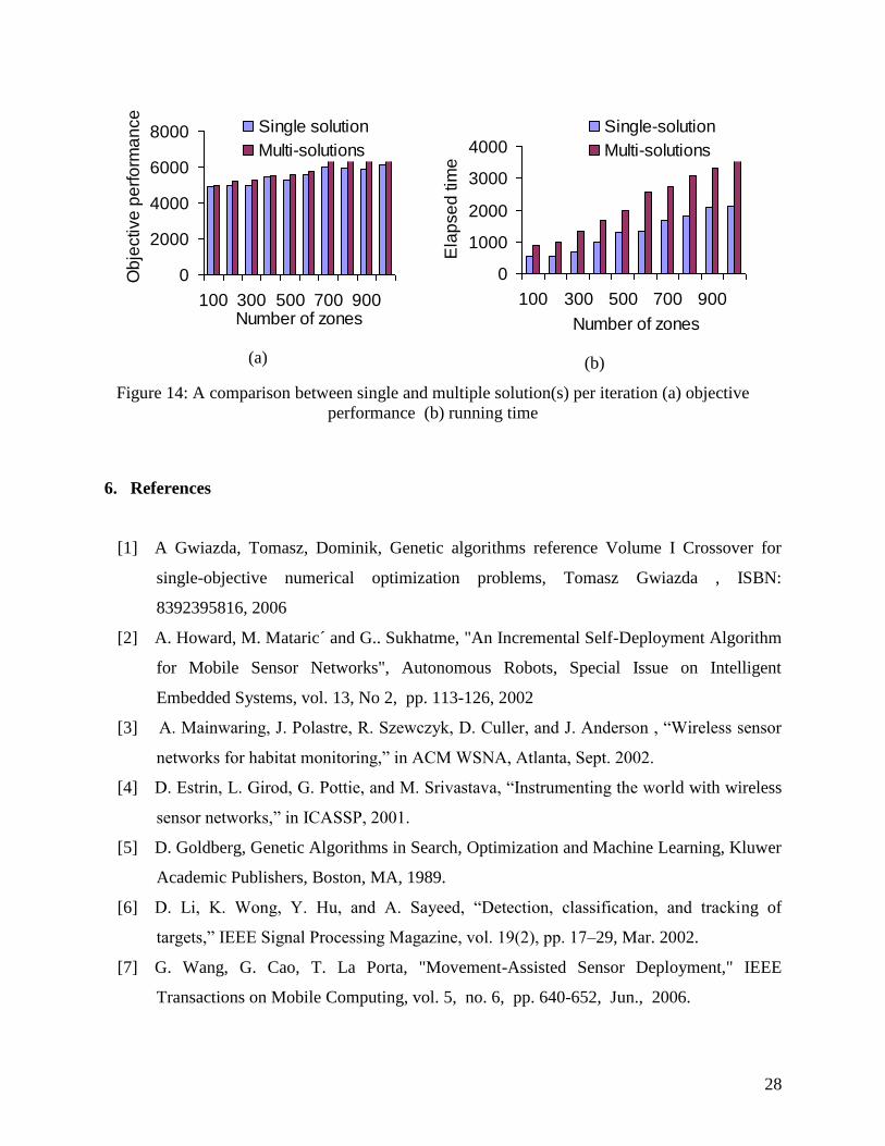
Two implementations are considered for the SA algorithm: single solution per iteration
and multiple solutions per iteration. Multiple solutions per iteration algorithm direct the search
26
into multiple search spaces. To compare these two implementations, problem settings of 50
sensors 12 time units and number of zones that range from 100 to 1000 zones. For the multiple
solutions case, 10 solutions per iteration are generated. The starting and final temperatures are set
to 2 and 1000, respectively. The temperature rate is assumed to be 0.99. As shown in Figure 14,
based on the conducted experiments, the multiple solutions implementation seems to outperform
the single solution. For example, for a problem with 1000 zones, the objective function of single
solution implementation is 10% less than that of the multiple solutions implementation. This
10% improvement in the coverage performance is associated with about 40% increase in the
running time.
5. Conclusions
A modeling framework for the problem of deploying a set of heterogeneous sensors in a
field with time-varying differential surveillance requirements is presented. In this framework, the
problem is formulated as a mixed integer mathematical program with the objective is to
maximize coverage of a given field. A set of constraints are defined to ensure that sensors are not
used beyond their capacity. Two meta-heuristics are also used to solve this problem. The first
heuristic adopts a Genetic Algorithm (GA) approach while the second heuristic implements a
Simulated Annealing (SA) algorithm. A set of experiments are used to illustrate capabilities of
the developed models and to compare their performance. The results indicate that both GA and
SA algorithms provide high quality solutions in terms of objective function and running time. In
addition, GA seems to yield better coverage performance than the SA. However, its running time
was always higher in all considered experimental settings.
27
8000
8500
9000
9500
10000
10500
0 20 40 60 80 100
Mutation percentage
Ob
jective
pe
rfro
ma
nce
Figure 12: GA performance with different mutation percentage
0
1000
2000
3000
4000
5000
6000
7000
8000
9000
0 32 64 96 128 160 192 224 256 288
Iterations
Ob
jective
r p
erf
orm
an
ce
Figure 13: Objective function progress with number of iterations
28
0
2000
4000
6000
8000
100 300 500 700 900Number of zones
Ob
jective
pe
rfo
rma
nce
Single solution
Multi-solutions
(a)
0
1000
2000
3000
4000
100 300 500 700 900
Number of zones
Ela
pse
d tim
e
Single-solution
Multi-solutions
(b)
Figure 14: A comparison between single and multiple solution(s) per iteration (a) objective
performance (b) running time
6. References
[1] A Gwiazda, Tomasz, Dominik, Genetic algorithms reference Volume I Crossover for
single-objective numerical optimization problems, Tomasz Gwiazda , ISBN:
8392395816, 2006
[2] A. Howard, M. Mataric´ and G.. Sukhatme, "An Incremental Self-Deployment Algorithm
for Mobile Sensor Networks", Autonomous Robots, Special Issue on Intelligent
Embedded Systems, vol. 13, No 2, pp. 113-126, 2002
[3] A. Mainwaring, J. Polastre, R. Szewczyk, D. Culler, and J. Anderson , “Wireless sensor
networks for habitat monitoring,” in ACM WSNA, Atlanta, Sept. 2002.
[4] D. Estrin, L. Girod, G. Pottie, and M. Srivastava, “Instrumenting the world with wireless
sensor networks,” in ICASSP, 2001.
[5] D. Goldberg, Genetic Algorithms in Search, Optimization and Machine Learning, Kluwer
Academic Publishers, Boston, MA, 1989.
[6] D. Li, K. Wong, Y. Hu, and A. Sayeed, “Detection, classification, and tracking of
targets,” IEEE Signal Processing Magazine, vol. 19(2), pp. 17–29, Mar. 2002.
[7] G. Wang, G. Cao, T. La Porta, "Movement-Assisted Sensor Deployment," IEEE
Transactions on Mobile Computing, vol. 5, no. 6, pp. 640-652, Jun., 2006.
29
[8] I. Akyildiz, W. Su, Y. Sankarasubramaniam, and E. Cayirci, "Wireless sensor networks:
A survey," Comput. Netw., vol. 38, pp. 393--422, 2002
[9] J. Lee, B. Krishnamachari and C. Kuo, “Impact of Heterogeneous Deployment on
Lifetime Sensing Coverage in Sensor Networks”, IEEE SECON, 2004.
[10] J. Lee, B. Krishnamachari, C.-C. Jay Kuo, "Node Aging Effect on Connectivity of Data
Gathering Trees in Sensor Networks" IEEE VTC, 2004
[11] J. O’Rourke, "Galleries Need Fewer Mobile Guards: A Variation on Chvatal’s Theorem",
Geometriae Dedicata ,vol. 14 , pp 273-283 ,1983.
[12] K. Chakrabarty, S. S. Iyengar, H. Qi and E. Cho, “Grid coverage for surveillance and
target Location in distributed sensor networks,” IEEE Transactions on Computers, vol.
51, pp. 1448–1453, 2002.
[13] L. Randy , S. Haupt, Practical Genetic Algorithms, Wiley, ISBN: 0-471-45565-2, 2004.
[14] M. Cardei and J. Wu, “Coverage in Wireless Sensor Networks,” in Handbook of Sensor
Networks, M.Ilyas and I. Mahgoub (eds.), CRC Press, ISBN 0-8493-1968-4, 2004.
[15] M. Ilyas and I. Mahgoub , Handbook of Sensor Networks, CRC Press, ISBN 0-8493-
1968-4, 2005.
[16] M. Kuorilehto, M., Hännikäinen, M., and Hämäläinen, T. D. 2005,” A survey of
application distribution in wireless sensor networks,” EURASIP J. Wirel. Commun.
Netw. , vol. 5, 774-788, 2005.
[17] N. Nguyen, S. Venkatesh, G. West, H. Bui, “Multiple camera coordination in a
surveillance system,” Acta Automatic Sinica, Vol. 29, No. 3, May, pp. 408-422, 2003.
[18] S. Dhillon, K. Chakrabarty and S.S. Iyengar, “Sensor placement for grid coverage under
imprecise detections,” Proc. International Conference on Information Fusion, pp. 1581–
1587, 2002.
[19] S. Kirkpatrick, C.D. Gelatt, M.P. Vecchi, ” Optimization by simulated annealing,”
Science , vol. 220, pp. 671–680, 1983.
[20] S. Poduri, Gaurav S. Sukhatme, “Constrained Coverage for Mobile Sensor Networks,”
IEEE International Conference on Robotics and Automation, New Orleans, LA, USA, pp.
165-172 , 2004.
[21] V. Chvatal, "A Combinatorial Theorem in Plane Geometry", Journal of Computorial
Theory (B), vol. 18, pp 39-41,1975.
30
[22] V. Isler, K. Daniilidis, and S. Kannan, “Sampling based sensor-network deployment,”
IEEE/RSJ International Conference on Intelligent Robots and Systems, 2004.
[23] W. Hu, C. Chou, S. Jha and N. Bulusu, "Deploying Long-lived and Cost-effective Hybrid
Sensor Networks," In Proceedings of the First Workshop on Broadband Advanced Sensor
Networks (BaseNets), San Diego, October 2004.
[24] W. Ye, J. Heidemann and D. Estrin. “An Energy- Efficient MAC Protocol for Wireless
Sensor Networks”, 21st Annual Joint Conference of the IEEE Computer and
Communications Societies (INFOCOM), vol. 3, pp 1567-1576, 2002
[25] X. Liu and P. Mahapatra, “On the deployment of wireless sensor nodes,” Third
International Workshop on Measurement, Modeling, and Performance Analysis of
Wireless Sensor Networks, in conjunction with MobiQuitous, ACM, 2005.
[26] Y. Xu, J. Heidemann, and D. Estrin, “Geography-informed Energy Conservation for Ad
Hoc Routing,” Proc. of Mobile Computing and Networking ( Mobicom ), pp. 70-84, July
2001.
[27] Y. Zou and K. Chakrabarty, "Sensor deployment and target localization in distributed
sensor networks", ACM Transactions on Embedded Computing Systems, vol. 3, pp. 61-
91, 2004.
[28] Y. Zou and K. Chakrabarty, "Sensor deployment and target localization based on virtual
forces", IEEE Infocom Conference, pp. 1293-1303, 2003.
Top Related