


Languages
Pages
Legal


OpenFOAM® Basic Training
3rd edition, Feb. 2015
This offering is not approved or endorsed by ESI® Group, ESI-OpenCFD® or the OpenFOAM® Foundation, the producer of the OpenFOAM® software and owner of the OpenFOAM® trademark.

Editors and Contributors:
Bahram Haddadi (TU Wien)
Christian Jordan (TU Wien)
Jozsef Nagy (JKU Linz)
Clemens Gößnitzer (TU Wien)
Vikram Natarajan (TU Wien)
Sylvia Zibuschka (TU Wien)
Michael Harasek (TU Wien)
Vienna University of Technology Institute of Chemical Engineering
Cover picture from:
Bahram Haddadi, The image presented on the cover page has been prepared
using the Vienna Scientific Cluster (VSC).
Attribution-NonCommercial-ShareAlike 3.0 Unported (CC BY-NC-SA 3.0)
This is a human-readable summary of the Legal Code (the full license). Disclaimer You are free:
to Share — to copy, distribute and transmit the work
to Remix — to adapt the work Under the following conditions:
Attribution — You must attribute the work in the manner specified by the author or licensor (but not in any way that suggests that they endorse you or your use of the work).
Noncommercial — You may not use this work for commercial purposes.
Share Alike — If you alter, transform, or build upon this work, you may distribute the resulting work only under the same or similar license to this one.
With the understanding that:
Waiver — Any of the above conditions can be waived if you get permission from the copyright holder.
Public Domain — Where the work or any of its elements is in the public domain under applicable law, that status is in no way affected by the license.
Other Rights — In no way are any of the following rights affected by the license:
Your fair dealing or fair use rights, or other applicable copyright exceptions and limitations;
The author's moral rights;
Rights other persons may have either in the work itself or in how the work is used, such as publicity or privacy rights.
Notice — For any reuse or distribution, you must make clear to others the license terms of this work. The best way to do this is with a link to this web page.
This book has been used as a basis for preparing a series of video lectures on youtube
by Jozsef Nagy (JKU Linz):
www.youtube.com/channel/UCjdgpuxuAxH9BqheyE82Vvw
(Search for: Jozsef Nagy OpenFOAM at youtube.com)
OpenFOAM
® Basic Training
Table of Contents
i
Tutorial One: elbow Page 1
Solver: icoFoam
Geometry: 2-dimensional
Purpose: Different meshes
Tutorial Two: forwardStep Page 11
Solver: sonicFoam
Geometry: 2-dimensional
Purpose: Built in meshing
Tutorial Three: shockTube Page 17
Solver: sonicFoam
Geometry: 1-dimensional
Purpose: Patching fields
Tutorial Four: shockTube Page 23
Solver: scalarTransportFoam
Geometry: 1-dimensional
Purpose: Discretization
Tutorial Five: circle Page 28
Solver: scalarTransportFoam
Geometry: 2-dimensional
Purpose: Discretization
Tutorial Six: pitzDaily Page 32
Solver: simpleFoam
Geometry: 2-dimensional
Purpose: Steady state, Turbulence
Tutorial Seven: pitzDaily Page 36
Solver: pisoFoam
Geometry: 2-dimensional
Purpose: Transient, Turbulence
Tutorial Eight: damBreak Page 40
Solver: interFoam
Geometry: 2-dimensional
Purpose: Multiphase

OpenFOAM
® Basic Training
Table of Contents
ii
Tutorial Nine: depthCharge3D Page 45
Solver: compressibleInterFoam
Geometry: 3-dimensional
Purpose: Parallel processing, Manual method in parallel processing
Tutorial Ten: TJunction Page 54
Solver: simpleFoam, scalarTransportFoam
Geometry: 3-dimensional
Purpose: Residence Time Distribution
Tutorial Eleven: reactingElbow Page 61
Solver: reactingFoam
Geometry: 3-dimensional
Purpose: Setting reacting simulations
Appendix A: Important Linux Commands Page 68
Appendix B: Running OpenFOAM® Page 71
Appendix C: Frequently Asked Questions (FAQ) Page 74
Appendix D: ParaView Page 77
OpenFOAM
® Basic Training
Example One
1
icoFoam – elbow (mesh)
Simulation
Using icoFoam solver, simulate 75 s of flow in an elbow for following GAMBIT
meshes:
Tri-mesh (comes with OpenFOAM® tutorial)
Hex-mesh coarse (check GAMBIT “elbow 2D” tutorial)
2 times finer hex-mesh (refine previous step mesh)
Objectives
Looking at the initial values for p and U.
Ensuring proper boundary definitions (imported boundaries from GAMBIT,
additional surfaces during conversion and boundaries definition in OpenFOAM®)
Post processing
Import your simulation to ParaView, extract data make two diagrams (using
spreadsheet calculators) of pressure and velocity magnitude along a line between two
tubes, do the same for all three simulations.

OpenFOAM
® Basic Training
Example One
2
Step by step simulation
Setting system environment
Make sure your system environment is set correctly, check Appendix B.
Copying tutorial
Open a terminal and copy the elbow tutorial from the following path to your working
directory (see Appendix A for using a terminal in Linux):
~/OpenFOAM/OpenFOAM-2.3.0/tutorials/incompressible/icoFoam/
elbow
Converting mesh
The mesh which is produced by GAMBIT is not directly compatible with
OpenFOAM®. First, the mesh needs to be converted to an OpenFOAM
® mesh, using
following tool:
>fluentMeshToFoam elbow.msh
If the mesh was created in mm and is converted using the mentioned command it will
convert the mesh with wrong dimensions, since all the units in OpenFOAM®
are SI1
Units. There are different flags included with most of OpenFOAM®
tools, for
checking them use the flag -help after the command, e.g.:
>fluentMeshToFoam –help
The output gives an overview of available options of the tool and also a short
description on how to use it:
Usage: fluentMeshToFoam [OPTIONS] <Fluent mesh file>
options:
-case <dir> specify alternate case directory, default is the cwd
-noFunctionObjects
do not execute functionObjects
-scale <factor> geometry scaling factor - default is 1
-writeSets write cell zones and patches as sets
-writeZones write cell zones as zones
-srcDoc display source code in browser
-doc display application documentation in browser
-help print the usage
Using: OpenFOAM-2.3.0 (see www.OpenFOAM.org)
Build: 2.3.0-f5222ca19ce6
The -scale flag is used for converting the mesh dimensions from other units to SI
units, e.g. if the mesh was created in mm it will be converted to meter by using -
scale 0.001 and if the flag is omitted, uses 1:
>fluentMeshToFoam elbow.msh -scale 1.0
Note: The mesh which is imported to OpenFOAM®
should be a three dimensional
mesh. For carrying out 2D (also 1D) simulations a three-dimensional mesh should be
1 International System of Units

OpenFOAM
® Basic Training
Example One
3
created with just one cell in the third dimension (for 1D, one cell in the second and
also one cell in the third direction).
Note: If there are internal boundaries in the mesh, there is another tool,
fluent3DMeshToFoam. Using this tool, the internal boundaries will be kept during
conversion.
Case structure
Most of the cases in OpenFOAM®
have the following basic case structure (directory
tree):
There are three main directories (0, constant, system) in each case foloder:
0 directory
The 0 directory includes the initial conditions for running the simulation. In each file
in this folder the initial conditions for one property can be set. The files are named
after the property they are standing for, e.g. usually T file includes temperature initial
conditions. In the elbow example there are only two files inside the 0 directory, p and
U. p stands for pressure and U stands for velocity. Checking p:
OpenFOAM
® Basic Training
Example One
4
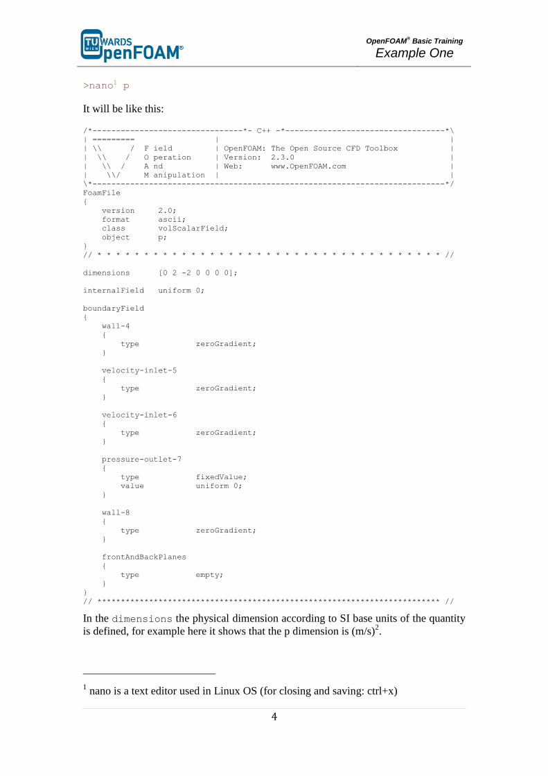
>nano1 p
It will be like this:
/*--------------------------------*- C++ -*----------------------------------*\
| ========= | |
| \\ / F ield | OpenFOAM: The Open Source CFD Toolbox |
| \\ / O peration | Version: 2.3.0 |
| \\ / A nd | Web: www.OpenFOAM.com |
| \\/ M anipulation | |
\*---------------------------------------------------------------------------*/
FoamFile
{
version 2.0;
format ascii;
class volScalarField;
object p;
}
// * * * * * * * * * * * * * * * * * * * * * * * * * * * * * * * * * * * * * //
dimensions [0 2 -2 0 0 0 0];
internalField uniform 0;
boundaryField
{
wall-4
{
type zeroGradient;
}
velocity-inlet-5
{
type zeroGradient;
}
velocity-inlet-6
{
type zeroGradient;
}
pressure-outlet-7
{
type fixedValue;
value uniform 0;
}
wall-8
{
type zeroGradient;
}
frontAndBackPlanes
{
type empty;
}
}
// ************************************************************************* //
In the dimensions the physical dimension according to SI base units of the quantity
is defined, for example here it shows that the p dimension is (m/s)2.
1 nano is a text editor used in Linux OS (for closing and saving: ctrl+x)

OpenFOAM
® Basic Training
Example One
5
Note: As you can see the p unit is not the pressure unit (Pa). It is due to the fact that
in incompressible solvers in OpenFOAM®
p is defined as “reduced” pressure divided
by density.
Note: In the dimension matrix the first number presents mass unit power, the second
one the length, the third one time, the forth one the temperature and the fifth one the
quantity (mole).
The internalField sets the initial field of a specific quantity in the solution
domain.
The type of each of our boundaries as well as the value of this quantity on the
boundaries is defined in the boundaryField. There are different types of boundary
conditions in OpenFOAM®:
- zeroGradient: Applies a zero gradient boundary type to this boundary
(Neumann boundary condition).
- fixedValue: Applies a fixed value to this boundary (Dirichlet boundary
condition).
- empty: It is for sides, which are vertical to the direction which is not going to
be considered (e.g. in 2D simulations these boundaries are vertical to the third
dimension). In this boundary type both of the sides vertical to one dimension
should be selected together and named as one boundary.
Note: If a fixedValue boundary condition with value equals $internalField is
used, it is equal to using zeroGradient, except zeroGradient applies the
boundary condition implicitly, but fixedValue with $internalField value
applies the boundary condition explicitly.
Note: In some mesh creation software like GAMBIT, empty boundary condition do not
exist. All the faces perpendicular to the direction which is not going to be considered
should be defined as a new boundary with type wall. After converting the mesh to
OpenFOAM®
mesh, modify that boundary in the file constant/polyMesh/ boundary,
and change its type from wall to empty, and also change inGroups from wall to empty.
The U file has to be defined via three components (since velocity is a vector): first one
stands for the x component, second one for the y component, and the third one for the
z component. For this case setup the z component is always zero because it is a 2D
simulation and no calculations will be done in the z direction. The boundaries vertical
to z direction have been already set to empty.
constant directory
The constant directory usually consists of a subdirectory and some files. The files
(usually) include material properties, simulation physics and chemistry. In the
directory “polyMesh” the mesh data are stored (in this case the data for converted
mesh). The boundary file in this polyMesh directory includes the mesh boundary data,
OpenFOAM
® Basic Training
Example One
6
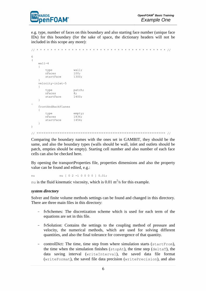
e.g. type, number of faces on this boundary and also starting face number (unique face
IDs) for this boundary (for the sake of space, the dictionary headers will not be
included in this scope any more):
// * * * * * * * * * * * * * * * * * * * * * * * * * * * * * * * * * * * * * //
6
(
wall-4
{
type wall;
nFaces 100;
startFace 1300;
}
velocity-inlet-5
{
type patch;
nFaces 8;
startFace 1400;
}
…
frontAndBackPlanes
{
type empty;
nFaces 1836;
startFace 1454;
}
)
// ************************************************************************* //
Comparing the boundary names with the ones set in GAMBIT, they should be the
same, and also the boundary types (walls should be wall, inlet and outlets should be
patch, empties should be empty). Starting cell number and also number of each face
cells can also be checked here.
By opening the transportProperties file, properties dimensions and also the property
value can be found and edited, e.g.:
nu nu [ 0 2 -1 0 0 0 0 ] 0.01;
nu is the fluid kinematic viscosity, which is 0.01 m2/s for this example.
system directory
Solver and finite volume methods settings can be found and changed in this directory.
There are three main files in this directory:
- fvSchemes: The discretization scheme which is used for each term of the
equations are set in this file.
- fvSolution: Contains the settings to the coupling method of pressure and
velocity, the numerical methods, which are used for solving different
quantities, and also the final tolerance for convergence of that quantity.
- controlDict: The time, time step from where simulation starts (startFrom),
the time when the simulation finishes (stopAt), the time step (deltaT), the
data saving interval (writeInterval), the saved data file format
(writeFormat), the saved file data precision (writePrecision), and also

OpenFOAM
® Basic Training
Example One
7
if changing the files during the run can affect the run or not
(runTimeModifiable) are set in this file.
Note: If the write format is ascii, then the simulation data which is written to the file
can be opened and read using any text editor. If the format is binary, the data will
be written in binary style and is not readable by text editors. The advantage of
binary over ascii is the smaller file size, and consequently faster conversion and
writing to disk, for big simulations.
// * * * * * * * * * * * * * * * * * * * * * * * * * * * * * * * * * * * * * //
application icoFoam;
startFrom latestTime;
startTime 0;
stopAt endTime;
endTime 75;
deltaT 0.05;
writeControl timeStep;
writeInterval 20;
purgeWrite 0;
writeFormat ascii;
writePrecision 6;
writeCompression uncompressed;
timeFormat general;
timePrecision 6;
runTimeModifiable yes;
// ************************************************************************* //
Note: This simulation continues from the last time step data which is saved
(latestTime). If there was no saved data it will start from start time (startTime),
which is zero in this case.
Running simulation
The simulation can be run by typing the solver‟s name and executing it:
>icoFoam
Note: For running the simulation the solver command (e.g. icoFoam) should be
executed inside the copy of the tutorial main folder. For example: The command
should be executed in the elbow folder, if it was run at some subfolders or somewhere
else, the simulation will fail.
OpenFOAM
® Basic Training
Example One
8
Exporting simulation data
The data files created by OpenFOAM®
should be exported (converted) by the
appropriate tools, to the post processing tools data format. For ParaView:
>foamToVTK
where VTK is the ParaView data format. This command should be also executed in
the case main directory, e.g. elbow. Here, ParaView is used as the post-processing
tool, for running it
>paraview &
Note: There is also another option to open the OpenFOAM®
simulation results with
ParaView without converting them to VTK; Create an empty text file in the main case
directory, name it <someName>.foam (e.g. foam.foam), and execute the following
command. This method is good for fast evaluation of the data in the middle of the
simulation or with a decomposed case in parallel simulations:
>paraview foam.foam &
Note: By putting & at the end of command, the command line will remain active and
ready for further inputs while that program is running.
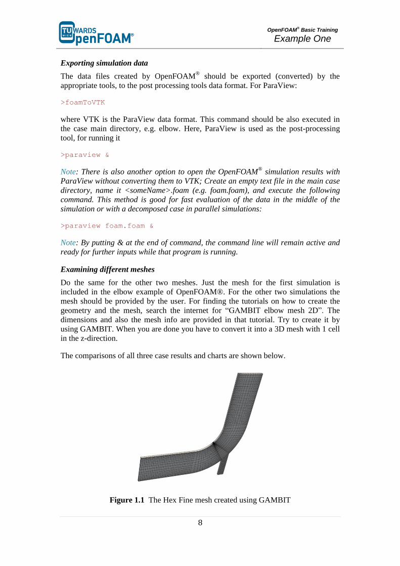
Examining different meshes
Do the same for the other two meshes. Just the mesh for the first simulation is
included in the elbow example of OpenFOAM®. For the other two simulations the
mesh should be provided by the user. For finding the tutorials on how to create the
geometry and the mesh, search the internet for “GAMBIT elbow mesh 2D”. The
dimensions and also the mesh info are provided in that tutorial. Try to create it by
using GAMBIT. When you are done you have to convert it into a 3D mesh with 1 cell
in the z-direction.
The comparisons of all three case results and charts are shown below.
Figure 1.1 The Hex Fine mesh created using GAMBIT
OpenFOAM
® Basic Training
Example One
9
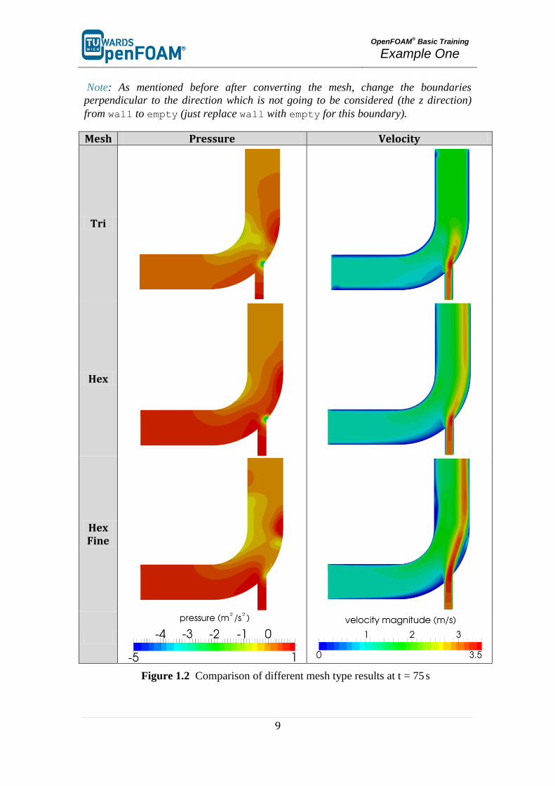
Note: As mentioned before after converting the mesh, change the boundaries
perpendicular to the direction which is not going to be considered (the z direction)
from wall to empty (just replace wall with empty for this boundary).
Mesh Pressure Velocity
Tri
Hex
Hex Fine
Figure 1.2 Comparison of different mesh type results at t = 75 s
OpenFOAM
® Basic Training
Example One
10
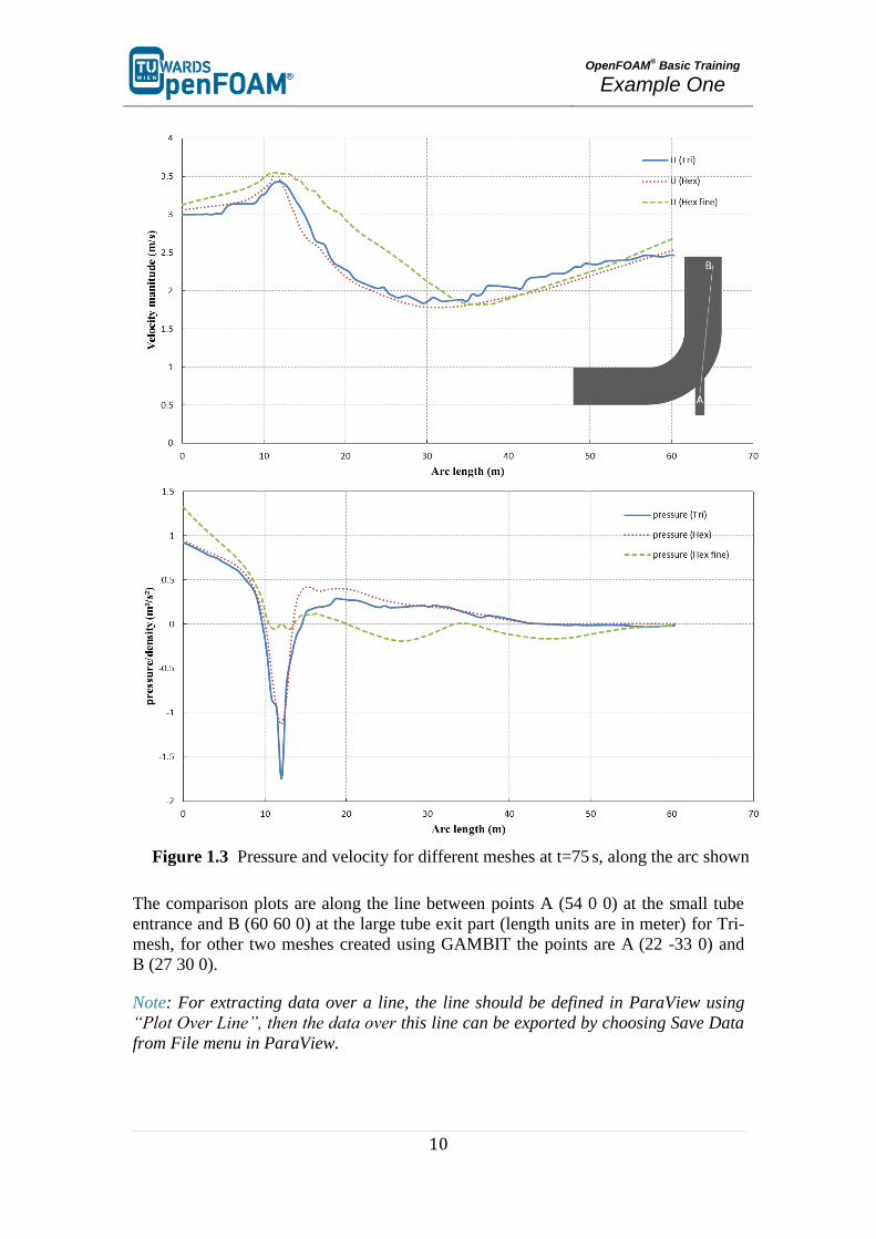
Figure 1.3 Pressure and velocity for different meshes at t=75 s, along the arc shown
The comparison plots are along the line between points A (54 0 0) at the small tube
entrance and B (60 60 0) at the large tube exit part (length units are in meter) for Tri-
mesh, for other two meshes created using GAMBIT the points are A (22 -33 0) and
B (27 30 0).
Note: For extracting data over a line, the line should be defined in ParaView using
“Plot Over Line”, then the data over this line can be exported by choosing Save Data
from File menu in ParaView.
OpenFOAM
® Basic Training
Example Two
11
sonicFoam – forwardStep
Simulation
Using sonicFoam solver, simulate 10 s of flow over a forward step.
Objectives
Understand blockMesh
Define vertices via coordinates as well as surfaces and volumes via vertices.
Post processing
Import your simulation into ParaView, and examine the mesh and the results in detail.
OpenFOAM
® Basic Training
Example Two
12
Step by step simulation
Copy tutorial
Copy the tutorial from the following folder to your working directory:
~/OpenFOAM/OpenFOAM-2.3.0/tutorials/compressible/sonicFoam/
laminar/forwardStep
0 directory
The file T includes the initial temperature values. Internal pressure and temperature
fields are set to 1, and the initial velocity in the domain is set to zero except at the
inlet boundary, where it is 3.
Note: As it can be seen, the p unit is the same as the pressure unit, because the
sonicFoam is a compressible solver.
Note: Do not forget that, this example is a purely numeric example (you might have
noticed this from pressure values).
constant directory
On checking thermophysicalProperties file, different properties of a compressible gas
can be set:
// * * * * * * * * * * * * * * * * * * * * * * * * * * * * * * * * * * * * * //
thermoType
{
type hePsiThermo;
mixture pureMixture;
transport const;
thermo hConst;
equationOfState perfectGas;
specie specie;
energy sensibleInternalEnergy;
}
mixture
{
specie
{
nMoles 1;
molWeight 11640.3;
}
thermodynamics
{
Cp 2.5;
Hf 0;
}
transport
{
mu 0;
Pr 1;
}
}
// ************************************************************************* //
In the thermoType, the models for calculating thermo physical properties of gas are
set:
OpenFOAM
® Basic Training
Example Two
13
- mixture: Is the model which is used for the mixture, whether it is a pure
mixture, a homogeneous mixture, a reacting mixture or ….
- transport: Defines the used transport model. In this example a constant
value is used.
- thermo: It defines the method for calculating heat capacities, e.g. in this
example constant heat capacities are used.
- equationOfState: Shows the relation which is used for the compressibility
of gases. Here ideal gas model is applied by selecting perfectGas.
- energy: This key word lets the solver decide which type of energy equation
it should solve, enthalpy or internal energy.
After defining the models for different thermo physical properties of gas, the
constants and coefficients of each model are defined in the sub-dictionary mixture.
E.g. molWeight shows the molecular weight of gas, Cp stands for heat capacity and
mu for dynamic viscosity as Pr shows the Prandtl number.
By opening the turbulenceProperties the appropriate turbulent mode can be set (in this
case it is laminar):
simulationType laminar;
There are two files in the polyMesh directory: blockMeshDict and boundary. In this
example the mesh is not imported from other programs (e.g. GAMBIT). It will be
created inside OpenFOAM®. For this purpose the blockMesh tool is used. blockMesh
reads the geometry and mesh properties from blockMeshDict file:
>nano blockMeshDict
// * * * * * * * * * * * * * * * * * * * * * * * * * * * * * * * * * * * * * //
convertToMeters 1;
vertices
(
(0 0 -0.05)
(0.6 0 -0.05)
(0 0.2 -0.05)
(0.6 0.2 -0.05)
(3 0.2 -0.05)
(0 1 -0.05)
(0.6 1 -0.05)
(3 1 -0.05)
(0 0 0.05)
(0.6 0 0.05)
(0 0.2 0.05)
(0.6 0.2 0.05)
(3 0.2 0.05)
(0 1 0.05)
(0.6 1 0.05)
(3 1 0.05)
);
blocks
(
hex (0 1 3 2 8 9 11 10) (25 10 1) simpleGrading (1 1 1)
hex (2 3 6 5 10 11 14 13) (25 40 1) simpleGrading (1 1 1)
hex (3 4 7 6 11 12 15 14) (100 40 1) simpleGrading (1 1 1)
);
OpenFOAM
® Basic Training
Example Two
14
edges
(
);
boundary
(
inlet
{
type patch;
faces
(
(0 8 10 2)
(2 10 13 5)
);
}
outlet
{
type patch;
faces
(
(4 7 15 12)
);
}
bottom
{
type symmetryPlane;
faces
(
(0 1 9 8)
);
}
top
{
type symmetryPlane;
faces
(
(5 13 14 6)
(6 14 15 7)
);
}
obstacle
{
type patch;
faces
(
(1 3 11 9)
(3 4 12 11)
);
}
);
mergePatchPairs
(
);
// ************************************************************************* //
As noted before units in OpenFOAM® are SI units. If the vertex coordinates differ
from SI, they can be converted with the convertToMeters command. The number
in the front of convertToMeters shows the constant, which should be multiplied
with the dimensions to change them to meter (SI unit of length). For example:
convertToMeters 0.001
shows that the dimensions are in millimeter, and by multiplying them by 0.001 they
are converted into meters.
OpenFOAM
® Basic Training
Example Two
15
In the vertices part, the coordinates of the geometry vertices are defined, the
vertices are stored and numbered from zero, e.g. vertex (0 0 -0.05) is numbered
zero, and vertex (0.6 1 -0.05) points to number 6.
In the block part, blocks are defined. The array of numbers in front each block shows
the block building vertices, e.g. the first block is made of vertices (0 1 3 2 8 9
11 10).
After each block the mesh is defined in every direction. e.g. (25 10 1) shows that
this block is divided into:
- 25 parts in x direction
- 10 parts in y direction
- 1 part in z direction
As it was explained before, even for 2D simulations the mesh and geometry should be
3D, but with one cell in the direction, which is not going to be solved, e.g. here
number of cells in z direction is one and it‟s because of that it‟s a 2D simulation in x-y
plane.
The last part, simpleGrading (1 1 1) shows the size function.
In the patches part each boundary is defined by the vertices it is made of, and also
its type and name are defined.
Note: For creating a face the vertices should be chosen clockwise when looking at the
face from inside of the geometry.
Running simulation
Before running the simulation the mesh has to be created. In the previous step the
mesh and the geometry data were set. For creating it the following command should
be executed from case main directory (e.g. forwardStep):
>blockMesh
After that, the mesh is created in the polyMesh folder. For running the simulation,
type the solver name form case directory and execute it:
>sonicFoam
Exporting simulation
The mesh is presented in the following way in ParaView, and you can easily see the
three blocks, which were created.
OpenFOAM
® Basic Training
Example Two
16
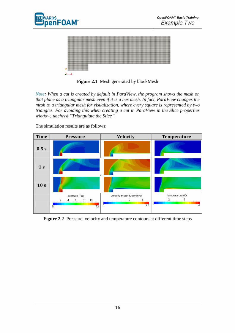
Figure 2.1 Mesh generated by blockMesh
Note: When a cut is created by default in ParaView, the program shows the mesh on
that plane as a triangular mesh even if it is a hex mesh. In fact, ParaView changes the
mesh to a triangular mesh for visualization, where every square is represented by two
triangles. For avoiding this when creating a cut in ParaView in the Slice properties
window, uncheck “Triangulate the Slice”.
The simulation results are as follows:
Time Pressure Velocity Temperature
0.5 s
1 s
10 s
Figure 2.2 Pressure, velocity and temperature contours at different time steps
OpenFOAM
® Basic Training
Example Three
17
sonicFoam – shockTube
Simulation
Use the sonicFoam solver, simulate 0.007 s of flow inside a shock tube, with a mesh
with 100, 1000 and 10000 cells in one dimension, for initial values 1 bar/0.1 bar and
10 bar/0.1 bar.
Objectives
Understanding setFields
Investigate effect of grid resolution
Post processing
Import your simulation into ParaView, and compare results.

OpenFOAM
® Basic Training
Example Three
18
Step by step simulation
Open tutorial
Copy the tutorial from the following directory to your working directory
~/OpenFOAM/OpenFOAM-2.3.0/tutorials/compressible/sonicFoam/
laminar/shockTube
constant directory
By checking the geometry and the mesh, it is obvious that it is a 1D mesh, because of
the number of mesh cells in y and z directions is one, and also in the patches, plates
vertical to these directions are defined as empty boundary condition. The mesh
density can be set in the blocks part by changing x direction mesh size (e.g. change
it from 1000 to 100 or 10000).
system directory
Checking system directory, there is a file “setFieldDict” which is used by the tool
setFields for patching (assign an amount to a region) in the simulation. For
example, here the pressure of 0.1 bar should be patched to half of the region (the
geometry is from -5 to 5, so from 0 to 5 will be patched) and 10 bar to the other half.
// * * * * * * * * * * * * * * * * * * * * * * * * * * * * * * * * * * * * * //
defaultFieldValues ( volVectorFieldValue U ( 0 0 0 ) volScalarFieldValue T
348.432 volScalarFieldValue p 1000000 );
regions ( boxToCell { box ( 0 -1 -1 ) ( 5 1 1 ) ; fieldValues (
volScalarFieldValue T 278.746 volScalarFieldValue p 10000 ) ; } );
// ************************************************************************* //
In the defaultFieldValues, a value is assigned to the whole domain, for example
here, the velocity has been set everywhere to zero, the temperature to 348.432 K, and
the pressure to 1000000 Pa. In the regions, boxToCell defines the region to which
a special amount must be patched. With boxToCell the region is chosen by a cube,
and the cube is defined by giving the coordinates of one of its diagonals.
After choosing the region, the new values are assigned to the parameters (e.g. here
temperature 278.746 K and pressure 10000 Pa).
Running simulation
In order to assign the values which were set in the setFieldDict:
>setFields
Then run:
>sonicFoam
Note: Checking deltaT in controlDict in the system directory, it is 1e-5 s. The
question is: What is the criteria for setting deltaT? If deltaT is bigger, the
simulation will run faster, but a too big deltaT makes the simulation unstable and

OpenFOAM
® Basic Training
Example Three
19
sometimes physically meaningless. Therefore deltaT should be selected in a way to
have a fast and at the same time stable and also physically reasonable simulation.
The Courant (Co) number is a dimensionless number, which is usually used as a
necessary condition for having a convergent solution, for one dimension:
Where u is velocity magnitude in that direction, Δt is deltaT and Δx is the mesh size
in this direction. For having a convergent solution in most of the cases Co should be
less than one in all the cells in the domain.
As it is obvious from the equation by decreasing the Δx or the mesh size deltaT
should be also adjusted (decreased) for having a stable and convergent solution.
In the OpenFOAM®
simulations usually Co is calculated in a way to make sure
maximum Courant number in the whole domain is less than 1. It is assumed Co = 1,
and for Δx smallest cell size and for u maximum velocity magnitude in domain is
selected. Then using these data, deltaT is calculated. It is a rough estimation, but
always helps to keep Co < 1!
Note: In the 10000 cell case with 10 bar and 0.1 bar, the simulation will crash with
the default deltaT (1e-5); After checking the same case with 1000 cells, you will
find that the maximum Co is around 0.6:
Time = 0.001
Courant Number mean: 0.0508555 max: 0.589018
diagonal: Solving for rho, Initial residual = 0, Final residual = 0, No
Iterations 0
In the case with 10000 cells, the number of cells is increased by factor 10, so the cell
size is reduced by factor 10. For keeping the Courant number in the same range
(around 0.6), according to the above equation, deltaT should be decreased by factor
10. After reducing it to 1e-6 the simulation will run smoothly.
Note: After running setFields for the first time, the files in the 0 directory are
overwritten. If the mesh will be changed these files are not compatible with the new
mesh and the simulation will fail. To solve this problem replace the files in the 0
directory with the files in the 0.org. In the OpenFOAM®
files or directories with suffix
“.org” (“original”) usually contain the backup files. If a command changes the
original files these files can be replaced.
Exporting simulation
The simulation results are as follows:

OpenFOAM
® Basic Training
Example Three
20
Figure 3.1 Velocities for different configurations along tube at t = 0.007 s
Figure 3.2 Velocity along tube axis for 10 bar/0.1bar and 10000 cells case at
t = 0.007 s
OpenFOAM
® Basic Training
Example Three
21
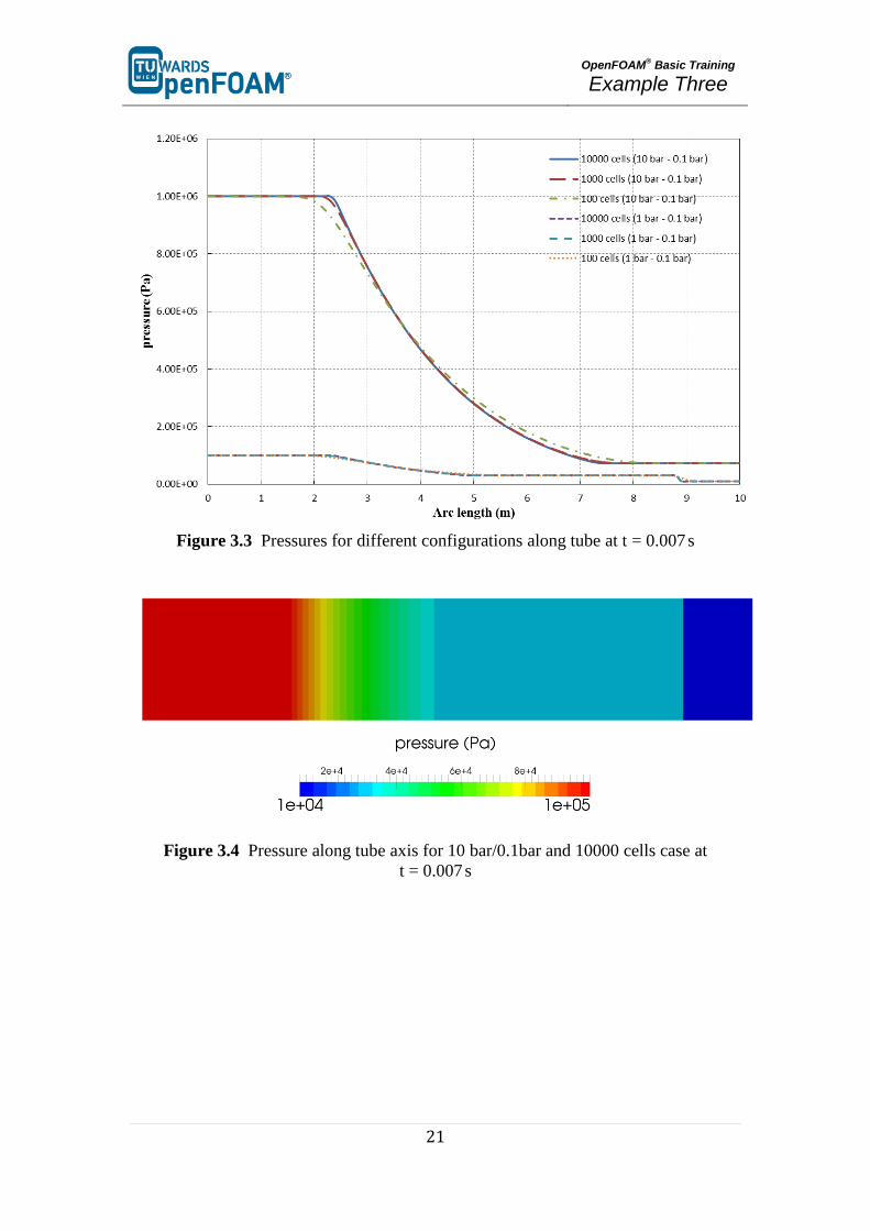
Figure 3.3 Pressures for different configurations along tube at t = 0.007 s
Figure 3.4 Pressure along tube axis for 10 bar/0.1bar and 10000 cells case at
t = 0.007 s

OpenFOAM
® Basic Training
Example Three
22
Figure 3.5 Temperature for different configurations along tube at t = 0.007 s
Figure 3.6 Temperature along tube axis for 10 bar/0.1bar and 10000 cells case at
t = 0.007 s

OpenFOAM
® Basic Training
Example Four
23
scalarTransportFoam – shockTube (discretization)
Simulation
Use the scalarTransportFoam solver, simulate 5 s of flow inside a shock tube, with 1D
mesh of 1000 cells (10 m long geometry from -5 m to 5 m). Patch with a scalar of 1
from -0.5 to 0.5. Simulate following cases:
Set U to uniform (0 0 0). Vary diffusion coefficient (low, medium and high
value).
Set the diffusion coefficient to zero and also U to (1 0 0) and run the
simulation in the case of pure advection using following discretization
schemes:
- upwind
- linear
- linearUpwind
- QUICK
- cubic
Objectives
Understanding different discretization schemes.
Post processing
Import your simulation into ParaView, and plot temperature along tube length.
OpenFOAM
® Basic Training
Example Four
24
Step by step simulation
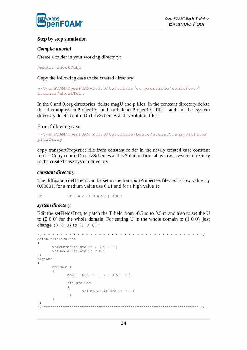
Compile tutorial
Create a folder in your working directory:
>mkdir shockTube
Copy the following case to the created directory:
~/OpenFOAM/OpenFOAM-2.3.0/tutorials/compressible/sonicFoam/
laminar/shockTube
In the 0 and 0.org directories, delete magU and p files. In the constant directory delete
the thermophysicalProperties and turbulenceProperties files, and in the system
directory delete controlDict, fvSchemes and fvSolution files.
From following case:
~/OpenFOAM/OpenFOAM-2.3.0/tutorials/basic/scalarTransportFoam/
pitzDaily
copy transportProperties file from constant folder in the newly created case constant
folder. Copy controlDict, fvSchemes and fvSolution from above case system directory
to the created case system directory.
constant directory
The diffusion coefficient can be set in the transportProperties file. For a low value try
0.00001, for a medium value use 0.01 and for a high value 1:
DT DT [ 0 2 -1 0 0 0 0] 0.01;
system directory
Edit the setFieldsDict, to patch the T field from -0.5 m to 0.5 m and also to set the U
to (0 0 0) for the whole domain. For setting U in the whole domain to (1 0 0), just
change (0 0 0) to (1 0 0):
// * * * * * * * * * * * * * * * * * * * * * * * * * * * * * * * * * * * * * //
defaultFieldValues
(
volVectorFieldValue U ( 0 0 0 )
volScalarFieldValue T 0.0
);
regions
(
boxToCell
{
box ( -0.5 -1 -1 ) ( 0.5 1 1 );
fieldValues
(
volScalarFieldValue T 1.0
);
}
);
// ************************************************************************* //
OpenFOAM
® Basic Training
Example Four
25
As it was mentioned before, the discretization scheme for each operator of the
governing equations can be set in fvSchemes.
// * * * * * * * * * * * * * * * * * * * * * * * * * * * * * * * * * * * * * //
ddtSchemes
{
default Euler;
}
gradSchemes
{
default Gauss linear;
}
divSchemes
{
default none;
div(phi,T) Gauss linearUpwind grad(T);
}
laplacianSchemes
{
default none;
laplacian(DT,T) Gauss linear corrected;
}
interpolationSchemes
{
default linear;
}
snGradSchemes
{
default corrected;
}
fluxRequired
{
default no;
T ;
}
// ************************************************************************* //
For each type of operation a default scheme can be set (e.g. for divSchemes is set to
none, it means no default scheme is set). Also a special type of discretization for each
element can be assigned (e.g. div(phi,T) it is set to linearUpwind). For each
element, which a discretization method has not been set, the default method will be
applied and if the default setting is none and no scheme is set for that element the
simulation will crash.
Note: The general transport equation for property φ looks like the following:
In this equation the first term shows the rate of change of property φ with time. The
second term is responsible for the advection of property φ by the fluid flow and the
third term shows the diffusion of property φ.
The right hand side of the equation also refers to the source terms. By setting the
diffusion coefficient (Γ, in this simulation it is DT) to zero, the case will be switched to
a pure advection simulation with no diffusion.
OpenFOAM
® Basic Training
Example Four
26
Note: In fvSchemes, the schemes for the time term of the general transport equation
are set in ddtSchemes sub-dictionary. divSchemes are responsible for the
advection term schemes and laplacianSchemes set the diffusion term schemes.
Note: divSchemes should be applied like this: Gauss + scheme. The Gauss keyword
specifies the standard finite volume discretization of Gaussian integration which
requires the interpolation of values from cell centers to face centers. Therefore, the
Gauss entry must be followed by the choice of interpolation scheme
(www.openfoam.org).
Running simulation
>blockMesh
>setFields
>scalarTransportFoam
Exporting simulation
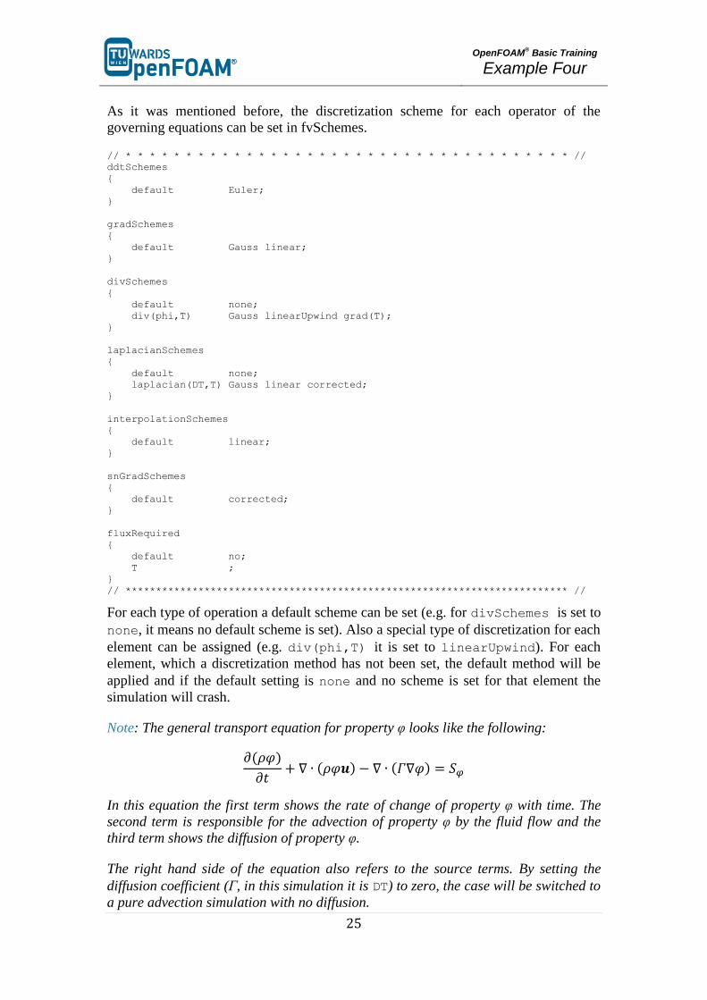
The simulation results are as follows.
A) Case with zero velocity (pure diffusion):
Figure 4.1 Pure diffusion with low diffusivity (0.00001) at t = 5 s
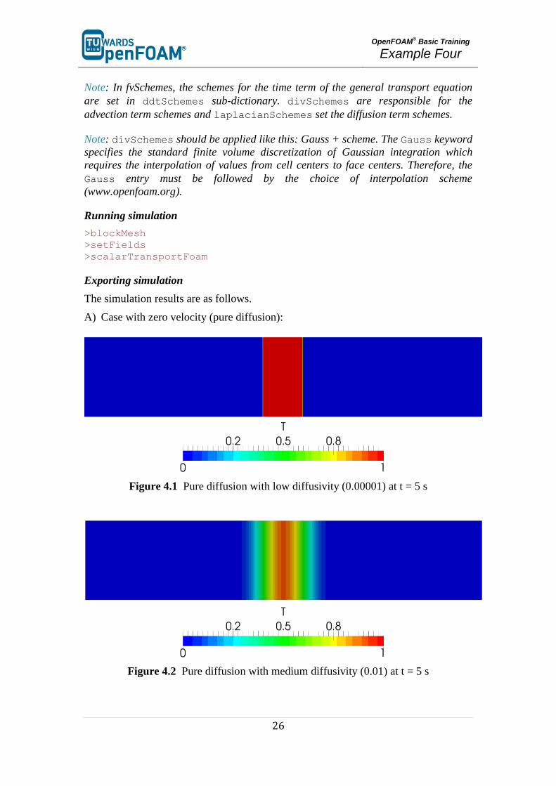
Figure 4.2 Pure diffusion with medium diffusivity (0.01) at t = 5 s
OpenFOAM
® Basic Training
Example Four
27
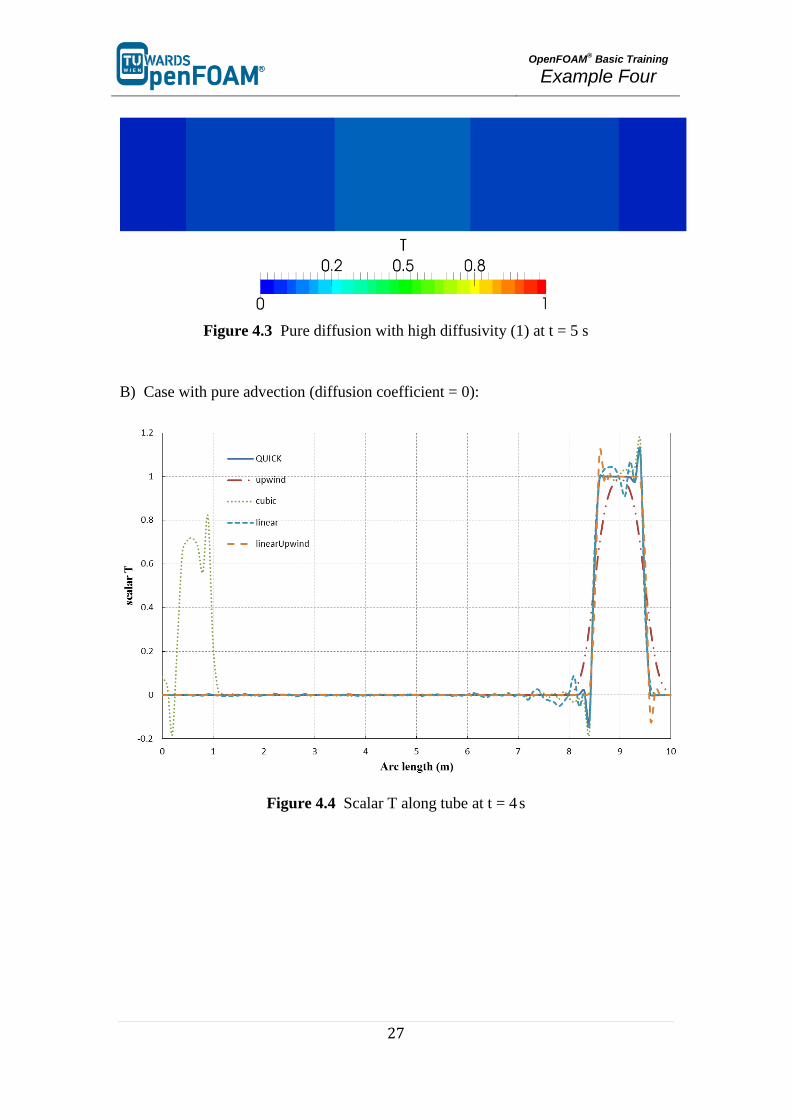
Figure 4.3 Pure diffusion with high diffusivity (1) at t = 5 s
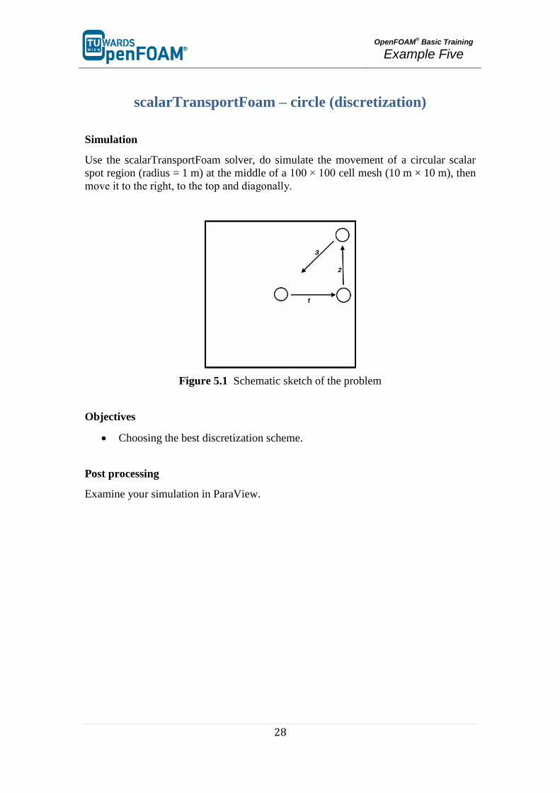
B) Case with pure advection (diffusion coefficient = 0):
Figure 4.4 Scalar T along tube at t = 4 s
OpenFOAM
® Basic Training
Example Five
28
scalarTransportFoam – circle (discretization)
Simulation
Use the scalarTransportFoam solver, do simulate the movement of a circular scalar
spot region (radius = 1 m) at the middle of a 100 × 100 cell mesh (10 m × 10 m), then
move it to the right, to the top and diagonally.
Figure 5.1 Schematic sketch of the problem
Objectives
Choosing the best discretization scheme.
Post processing
Examine your simulation in ParaView.

OpenFOAM
® Basic Training
Example Five
29
Step by step simulation
Compile tutorial
Create the new case in your working directory like in example four.
0 directory
To move the circle to right change the internalField to (1 0 0) in the U file for
setting the velocity field towards right for moving the circle to the right. Modify U at
suitable times, to obtain a velocity field which will move the circle up and also
diagonally.
constant directory
In the polyMesh directory, modify the blockMeshDict for creating a 2D geometry
with 100 × 100 cells mesh.
// * * * * * * * * * * * * * * * * * * * * * * * * * * * * * * * * * * * * * //
convertToMeters 1;
vertices
(
(-5 -5 -0.01)
(5 -5 -0.01)
(5 5 -0.01)
(-5 5 -0.01)
(-5 -5 0.01)
(5 -5 0.01)
(5 5 0.01)
(-5 5 0.01)
);
blocks
(
hex (0 1 2 3 4 5 6 7) (100 100 1) simpleGrading (1 1 1)
);
edges
(
);
boundary
(
sides
{
type patch;
faces
(
(1 2 6 5)
(0 4 7 3)
(3 7 6 2)
(0 1 5 4)
);
}
empty
{
type empty;
faces
(
(5 6 7 4)
(0 3 2 1)
);
}
);
// ************************************************************************* //
In the transportProperties set DT to zero (no diffusion!).

OpenFOAM
® Basic Training
Example Five
30
system directory
Choose a discretization scheme based on the results from the previous example and
set the fvSchemes.
In the setFieldDict patch a circle to the middle of the geometry using the following
lines.
// * * * * * * * * * * * * * * * * * * * * * * * * * * * * * * * * * * * * * //
defaultFieldValues (volScalarFieldValue T 0 );
regions
(
cylinderToCell
{
p1 ( 0 0 -1 );
p2 ( 0 0 1 );
radius 0.5;
fieldValues
(
volScalarFieldValue T 1
) ;
}
);
// ************************************************************************* //
cylinderToCell command is used to patch a cylinder to the region, p1 and p2
show the two ends of cylinder center line, in the radius the radius is set.
Check controlDict, in the first part of simulation, where the circle should move to the
right set the startFrom to startTime and startTime to 0. By a simple
calculation it can be seen that the endTime should be 3 s. Similar calculations need to
be done for the two other parts, except the startTime is set to the endTime of
previous part, and new endTime should be that part “simulation time” plus endTime
of the previous part.
Running simulation
>blockMesh
>setFields
>scalarTransportFoam
For running the further parts (moving the circle to top, and then diagonally) change
the velocity field in the last time step directory.
After moving the circle to the right and changing the velocity field, the simulation is
resumed. It can be seen that the circle does not go up but moves to the right. This
occurs due to the fact that OpenFOAM® used the previous time step fluxes (phi) to
do the calculations. We can solve this problem by deleting phi file from the latest time
step (of the previous part of simulation, e.g. 3). In this way, OpenFOAM® creates
new fluxes based on the new velocity field that we just updated. So, easily delete phi
and enjoy!

OpenFOAM
® Basic Training
Example Five
31
Exporting simulation
The simulation results are as follows:
1 s 2 s 3 s
4 s 5 s 6 s
7 s 8 s 9 s
Figure 5.2 Position of the circle at different time steps
OpenFOAM
® Basic Training
Example Six
32
simpleFoam – pitzDaily (turbulence, steady state)
Simulation
Use simpleFoam solver, run a steady state simulation with following turbulence
models:
kEpsilon (RAS)
kOmega (RAS)
LRR (RAS)
Objectives
Understanding turbulence modeling
Understanding steady state simulation
Post processing
Show the results of U and the turbulent viscosity in two separate contour plots.
OpenFOAM
® Basic Training
Example Six
33
Step by step simulation
Copy tutorial
~/OpenFOAM/OpenFOAM-2.3.0/tutorials/incompressible/simpleFoam
/pitzDaily
0 directory
When a turbulent model is chosen, the value of its constants and its boundary values
should be set in the appropriate files. For example in kEpsilon model the k and
epsilon files should be edited, e.g. epsilon:
// * * * * * * * * * * * * * * * * * * * * * * * * * * * * * * * * * * * * * //
dimensions [0 2 -3 0 0 0 0];
internalField uniform 14.855;
boundaryField
{
inlet
{
type fixedValue;
value uniform 14.855;
}
outlet
{
type zeroGradient;
}
upperWall
{
type epsilonWallFunction;
value uniform 14.855;
}
lowerWall
{
type epsilonWallFunction;
value uniform 14.855;
}
frontAndBack
{
type empty;
}
}
// ************************************************************************* //
Note: Here is a list of files which should be available at 0 directory and need to be
modified for each turbulence model:
laminar: no file
kEpsilon (RAS): k and epsilon
kOmega (RAS): k and omega
LRR (RAS): k, epsilon and R
Smagorinsky (LES): nuSgs
oneEqEddy (LES): k and nuSgs
OpenFOAM
® Basic Training
Example Six
34
SpalartAllmaras (LES): nuSgs and nuTilda
Some files are available, e.g. epsilon, k and nuTilda, some files should be created by
the user, e.g. R, omega. Templates for these files can be also found in the examples of
older versions of OpenFOAM®, e.g. 1.7.1.
Note: A missing R file can be created by OpenFOAM®
. In the constant directory in
RASProperties file set the RASModel to kEpsilon. The turbulenceProperties file is
also needed. Copy it from another tutorial and set simulationType to RASModel
in the file. Run the command “R” from terminal, it will create the R file in the 0
directory.
constant directory
The type of simulation turbulence model is set in turbulenceProperties file, e.g. it is a
RASModel or LESModel (this file is not available in this tutorial, but can be copied
from other tutorials). For choosing a specific turbulence model the RASProperties file
should be checked (e.g. here kEpsilon).
// * * * * * * * * * * * * * * * * * * * * * * * * * * * * * * * * * * * * * //
RASModel kEpsilon;
turbulence on;
printCoeffs on;
// ************************************************************************* //
Note: For the laminar model both turbulenceProperties and RASProperties should be
set to laminar. In the RASProperties set turbulence and also printCoeffs to
off.
system directory
Note: Since it is a steady state simulation in controlDict endTime shows the number
of iterations instead of time and deltaT should be 1, because it is the amount of
increase in the iteration number.
Running simulation
>blockMesh
>simpleFoam
Note: When the solution converges, “SIMPLE solution converged in …
iterations” message will be displayed in the Shell window. If nothing happens and
you do not see a message after a while (this is not the case in here, it converges after
a short time), then you should check the residuals which are displayed in the Shell
window manually (you should check initial residual values, it shows the
difference between this iteration and the last one), if all of the Initial residual
(see below) values are close to amounts you have set in the fvSolution then you can
stop simulation (ctrl+c).

OpenFOAM
® Basic Training
Example Six
35
Time = 817
smoothSolver: Solving for Ux, Initial residual = 0.00013826, Final residual =
9.87886e-06, No Iterations 2
smoothSolver: Solving for Uy, Initial residual = 0.000994709, Final residual =
7.317e-05, No Iterations 2
GAMG: Solving for p, Initial residual = 0.00192871, Final residual =
0.000174838, No Iterations 7
time step continuity errors : sum local = 0.000840075, global = 6.13868e-05,
cumulative = -0.193739
smoothSolver: Solving for epsilon, Initial residual = 0.000175322, Final
residual = 1.138e-05, No Iterations 2
smoothSolver: Solving for k, Initial residual = 0.000404928, Final residual =
2.99083e-05, No Iterations 2
ExecutionTime = 20.11 s ClockTime = 20 s
SIMPLE solution converged in 817 iterations
Exporting simulation
The simulation results are as follows (all simulations scaled to the same range):
RAS model
Velocity magnitude Turbulent viscosity
kEpsilon
kOmega
LRR
Figure 6.1 Comparison of different turbulent models at steady state

OpenFOAM
® Basic Training
Example Seven
36
pisoFoam – pitzDaily (turbulence, transient)
Simulation
Use the pisoFoam solver, run a backward facing step case for 0.2 s with different
turbulence models:
Smagorinsky (LES)
oneEqEddy (LES)
kEpsilon (RAS)
Objectives
Understanding turbulence models
Understanding the difference between transient and steady state simulation
Finding appropriate turbulence model
Post processing
Display the results of U and the turbulent viscosity in two separate contour plots at
three different time steps. Compare with steady state simulation (example 6).
OpenFOAM
® Basic Training
Example Seven
37
Step by step simulation
Copy tutorial
Copy the tutorial from the following directory to your working directory:
~/OpenFOAM/OpenFOAM-2.3.0/tutorials/incompressible/pisoFoam
/les/pitzDaily
0 directory
Set the turbulence model initial and boundary values.
Note: For different turbulent models, different constant files should be modified
(check example 6).
constant directory
As mentioned in example 6, in turbulenceProperties the turbulent model type has to
be set.
// * * * * * * * * * * * * * * * * * * * * * * * * * * * * * * * * * * * * * //
simulationType LESModel;
// ************************************************************************* //
For setting a turbulence model, if RAS models are being used, in the constant
directory there is the RASProperties file and we should modify it, but if LES models
are used the LESProperties file should be found and modified.
// * * * * * * * * * * * * * * * * * * * * * * * * * * * * * * * * * * * * * //
LESModel oneEqEddy;
delta cubeRootVol;
printCoeffs on;
cubeRootVolCoeffs
{
deltaCoeff 1;
}
PrandtlCoeffs
{
delta cubeRootVol;
cubeRootVolCoeffs
{
deltaCoeff 1;
}
smoothCoeffs
{
delta cubeRootVol;
cubeRootVolCoeffs
{
deltaCoeff 1;
}
maxDeltaRatio 1.1;
}
Cdelta 0.158;
OpenFOAM
® Basic Training
Example Seven
38
}
vanDriestCoeffs
{
delta cubeRootVol;
cubeRootVolCoeffs
{
deltaCoeff 1;
}
smoothCoeffs
{
delta cubeRootVol;
cubeRootVolCoeffs
{
deltaCoeff 1;
}
maxDeltaRatio 1.1;
}
Aplus 26;
Cdelta 0.158;
}
smoothCoeffs
{
delta cubeRootVol;
cubeRootVolCoeffs
{
deltaCoeff 1;
}
maxDeltaRatio 1.1;
}
// ************************************************************************* //
Running simulation
>blockMesh
>pisoFoam
Exporting simulation
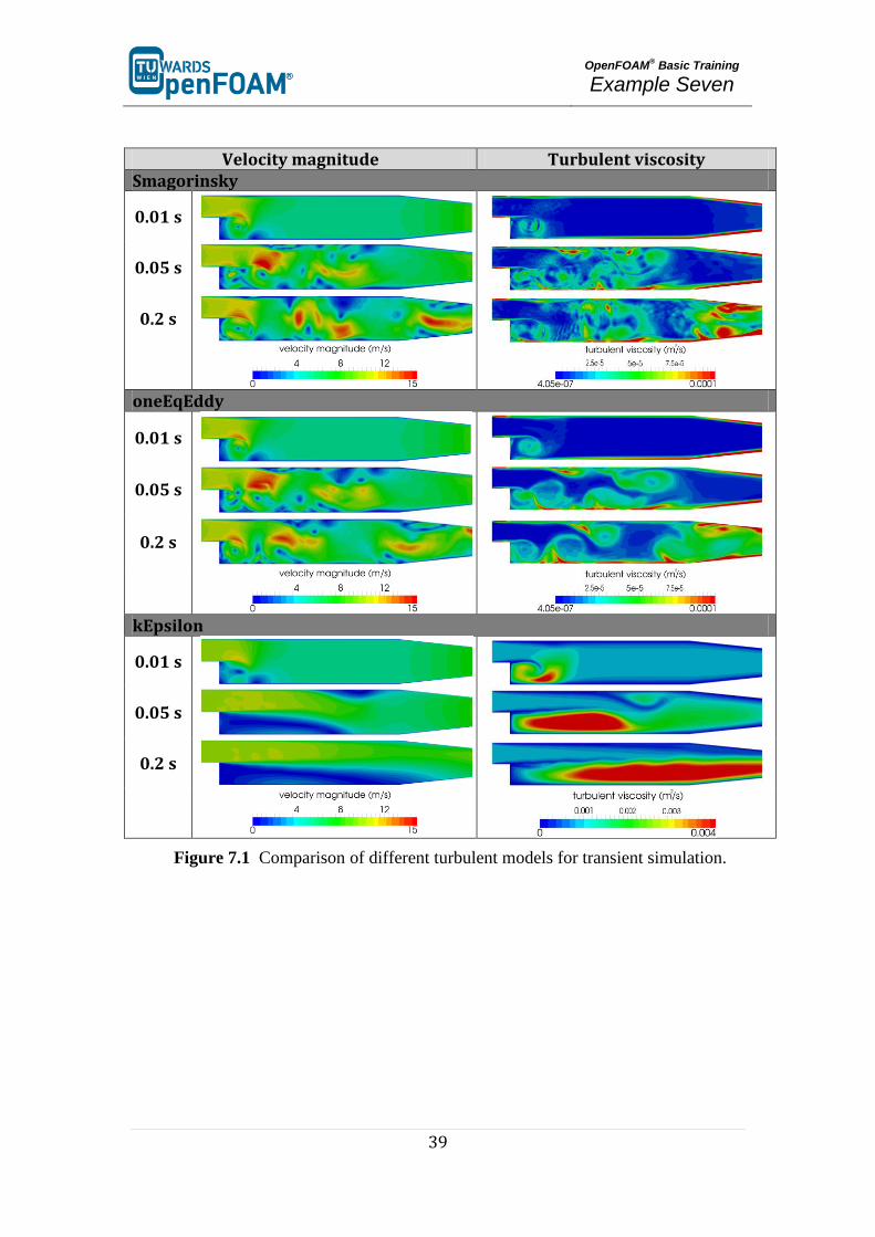
The simulation results are as follows:
For the kEpsilon model after 0.2 s the results are similar to the steady state simulation.
Therefore, it can be assumed it has reached the steady state. Other models do not have
a steady situation and are fluctuating all the time, so they require averaging for
obtaining steady state results.
kEpsilon and other RAS models use averaging to obtain the turbulence values, but
LES does not include any averaging by default. Therefore, LES simulations should
use a higher grid resolution (smaller cells) and smaller time steps (for reasonable Co
number). Contour plots or other LES results should be presented time averaged over
reasonable number of time steps (not done in this example).
OpenFOAM
® Basic Training
Example Seven
39
Velocity magnitude Turbulent viscosity
Smagorinsky
0.01 s
0.05 s
0.2 s
oneEqEddy
0.01 s
0.05 s
0.2 s
kEpsilon
0.01 s
0.05 s
0.2 s
Figure 7.1 Comparison of different turbulent models for transient simulation.

OpenFOAM
® Basic Training
Example Eight
40
interFoam – damBreak (multiphase)
Simulation
Use the interFoam solver to simulate breaking of a dam for 2s.
Objectives
Understanding how to set viscosity, surface tension and density for two phases
Post processing
See the results in ParaView.

OpenFOAM
® Basic Training
Example Eight
41
Step by step simulation
Copy tutorial
Copy tutorial from the following folder to your working directory:
~/OpenFOAM/OpenFOAM-2.3.0/tutorials/multiphase/interFoam
/laminar/damBreak
0 directory
In the 0 directory following files exist:
alpha.water.org p_rgh U
In the alpha.water.org and p_rgh files the initial values and also boundary conditions
for phase water and also pressure are set. Copy alpha.water.org to alpha.water
(remember: the *.org files are back up files, and solvers do not use them). E.g.
alpha.water:
// * * * * * * * * * * * * * * * * * * * * * * * * * * * * * * * * * * * * * //
dimensions [0 0 0 0 0 0 0];
internalField uniform 0;
boundaryField
{
leftWall
{
type zeroGradient;
}
rightWall
{
type zeroGradient;
}
lowerWall
{
type zeroGradient;
}
atmosphere
{
type inletOutlet;
inletValue uniform 0;
value uniform 0;
}
defaultFaces
{
type empty;
}
}
// ************************************************************************* //
Note: The inletOutlet and the outletInlet boundary conditions are used when
the flow direction is not known. In fact, these are derived types and are a combination
of two different boundary types.

OpenFOAM
® Basic Training
Example Eight
42
- inletOutlet: When the flux direction is toward the outside of the domain, it
works like a zeroGradient boundary condition and when the flux is toward
inside the domain it is like a fixedValue boundary condition.
- outletInlet: This is the other way around, if the flux direction is toward
outside the domain, it works like a fixedValue boundary condition and when
the flux is toward inside the domain, it is like a zeroGradient boundary
condition.
E.g. if the velocity field outlet is set as inletOutlet and the inletValue is set to
(0 0 0), it avoids backflow at the outlet! The “inletValue” or “outletValue”
are values for fixedValue type of these boundary conditions and “value” is a
dummy entery for OpenFOAM®
for finding the variable type. Using (0 0 0),
OpenFOAM®
understands that the variable is a vector.
constant directory
In the transportProperties file the properties of two phases can be set under each phase
sub-dictionary, e.g. water or air:
// * * * * * * * * * * * * * * * * * * * * * * * * * * * * * * * * * * * * * //
phases (water air);
water
{
transportModel Newtonian;
nu nu [ 0 2 -1 0 0 0 0 ] 1e-06;
rho rho [ 1 -3 0 0 0 0 0 ] 1000;
CrossPowerLawCoeffs
{
nu0 nu0 [ 0 2 -1 0 0 0 0 ] 1e-06;
nuInf nuInf [ 0 2 -1 0 0 0 0 ] 1e-06;
m m [ 0 0 1 0 0 0 0 ] 1;
n n [ 0 0 0 0 0 0 0 ] 0;
}
BirdCarreauCoeffs
{
nu0 nu0 [ 0 2 -1 0 0 0 0 ] 0.0142515;
nuInf nuInf [ 0 2 -1 0 0 0 0 ] 1e-06;
k k [ 0 0 1 0 0 0 0 ] 99.6;
n n [ 0 0 0 0 0 0 0 ] 0.1003;
}
}
air
{
transportModel Newtonian;
nu nu [ 0 2 -1 0 0 0 0 ] 1.48e-05;
rho rho [ 1 -3 0 0 0 0 0 ] 1;
CrossPowerLawCoeffs
{
nu0 nu0 [ 0 2 -1 0 0 0 0 ] 1e-06;
nuInf nuInf [ 0 2 -1 0 0 0 0 ] 1e-06;
m m [ 0 0 1 0 0 0 0 ] 1;
n n [ 0 0 0 0 0 0 0 ] 0;
}
BirdCarreauCoeffs
{
nu0 nu0 [ 0 2 -1 0 0 0 0 ] 0.0142515;
nuInf nuInf [ 0 2 -1 0 0 0 0 ] 1e-06;
OpenFOAM
® Basic Training
Example Eight
43
k k [ 0 0 1 0 0 0 0 ] 99.6;
n n [ 0 0 0 0 0 0 0 ] 0.1003;
}
}
sigma sigma [ 1 0 -2 0 0 0 0 ] 0.07;
// ************************************************************************* //
In both phases the coefficients for different models of viscosity are given, e.g. nu,
CrossPowerLawCoeffs and BirdCarreauCoeffs.
Depending on which model is selected, the coefficients from the corresponding sub-
dictionary are read. The selected model is Newtonian, only the nu coefficient is used
and the others remain unused (CrossPowerLawCoeffs and
BirdCarreauCoeffs).
sigma is the surface tension between two phases, in this example it is the surface
tension between air and water.
Checking the g file, the gravitational field and also its direction are defined, it is
9.81 m/s2 in the negative y direction.
// * * * * * * * * * * * * * * * * * * * * * * * * * * * * * * * * * * * * * //
dimensions [0 1 -2 0 0 0 0];
value ( 0 -9.81 0 );
// ************************************************************************* //
Running simulation
>blockMesh
>setFields
>interFoam
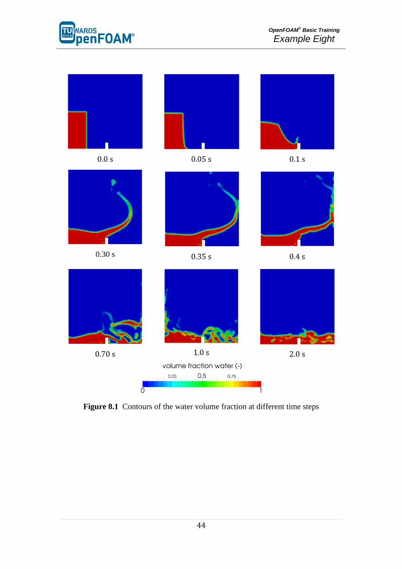
Exporting simulation
The simulation results are as follows (these are not the results for the original mesh,
but a 2x refined finer mesh):
OpenFOAM
® Basic Training
Example Eight
44
0.0 s
0.05 s
0.1 s
0.30 s
0.35 s
0.4 s
0.70 s
1.0 s
2.0 s
Figure 8.1 Contours of the water volume fraction at different time steps

OpenFOAM
® Basic Training
Example Nine
45
compressibleInterFoam – depthCharge3D
Simulation
Use the compressibleInterFoam solver, simulate the example case for 0.5 s.
Objectives
Understanding the difference between incompressible and compressible
solvers
Understanding parallel processing and different discretization methods
Post processing
Investigate the results in ParaView.
OpenFOAM
® Basic Training
Example Nine
46
Step by step simulation
Copy tutorial
Copy the tutorial from following directory to your working directory:
~/OpenFOAM/OpenFOAM-2.3.0/tutorials/multiphase/
compressibleInterFoam/laminar/depthCharge3D
0 directory
Copy alpha.water.org, p_rgh.org, p.org and T.org to alpha.water, p_rgh, p and T files.
constant directory
Phases and common physical properties of the two phases are set in the
thermophysicalProperties file. Individual phase properties are set in
thermophysicalProperties.phase files, e.g. thermophysicalProperties.air.
// * * * * * * * * * * * * * * * * * * * * * * * * * * * * * * * * * * * * * //
phases (water air);
pMin pMin [ 1 -1 -2 0 0 0 0 ] 10000;
sigma sigma [ 1 0 -2 0 0 0 0 ] 0.07;
// ************************************************************************* //
system directory
The decomposeParDict file includes the parallel settings, such as the number of
domains (partitions) and also how the domain is going to be divided into these
subdomains for parallel processing.
// * * * * * * * * * * * * * * * * * * * * * * * * * * * * * * * * * * * * * //
numberOfSubdomains 4;
method hierarchical;
simpleCoeffs
{
n ( 1 4 1 );
delta 0.001;
}
hierarchicalCoeffs
{
n ( 1 4 1 );
delta 0.001;
order xyz;
}
manualCoeffs
{
dataFile "";
}
distributed no;
roots ( );
// ************************************************************************* //
OpenFOAM
® Basic Training
Example Nine
47
numberOfSubdomains should equal the number of cores used. method should
show the method to be used. In the above example, the case is simulated with the
hierarchical method and 4 processors.
If the simple method is being used, the parameter n must be changed accordingly.
The three numbers (1 4 1) indicate the number of pieces the mesh is split into in
the x, y and z directions, respectively. Their multiplication result should be equal to
numberOfSubdomains.
If the hierarchical method is being used, these parameters and also the order in
which the mesh should be split up in each direction should be provided.
If the scotch method is being used, then no user-supplied parameters are necessary
except for the number of subdomains.
There is also a parameter delta, known as the cell skew factor. This factor is set to a
default value of 0.001, and measures to what extent skewed cells should be
accounted for.
Note: In order to check the quality of the mesh, the checkMesh tool can be used (run it
from main case directory). If the message “Mesh OK” is displayed – the mesh is fine
and no corrections need to be done.
If the mesh fails in one or more tests, try to recreate or refine the mesh for a better
mesh quality (less non-orthogonally and skewness). If the error exists after correcting
the mesh then a possible course of action is to increase the delta parameter (for
example: to 0.01) and then rerun the blockMesh and checkMesh tools.
If non-orthogonal cells exist in a mesh, another option is using non-orthogonal
corrections in the fvSolution file in the algorithm sub-dictionary (e.g. PIMPLE or
PISO). Usually using 1 or 2 as nNonOrthogonalCorrectors is enough.
Running simulation
>blockMesh
>setFields
For running the simulation in parallel mode the computing domain needs to be
divided into subdomains and a core should be assigned to each subdomain. This is
done by following command:
>decomposePar
This decomposes the mesh according to the supplied instructions. One possible source
of error is the product of the parameters in n does not match up to the number of the
subdomains. This appears for the simple and hierarchical methods.
After executing this command four new directories will be made in the simulation
directory (processor0, processor1, processor2 processor3), and each subdomain
calculation will be saved in the respective processor directory.
OpenFOAM
® Basic Training
Example Nine
48
Note: When the domain is divided to subdomains in parallel processing new
boundaries are defined. The data should be exchanged with the neighbor boundary,
which it is connected to in the main domain.
>mpirun -np <No of cores> solver –parallel > log
<No of cores> is the number of cores being used. solver is the solver for this
simulation. For example, if 4 cores are desired, and the solver is
compressibleInterFoam following command is used:
>mpirun -np 4 compressibleInterFoam -parallel > log
> log is the filename for saving the simulation status data, instead of printing them
to the screen. For checking the last information which is written to this file the
following command can be used during the simulation running:
>tail –f log
Note: Before running any simulation, it is important to run the top command (type the
top command in the terminal), to check the number of cores currently used on the
machine. Check the load average. This is on the first line and shows the average
number of cores being used. There are three numbers displayed, showing the load
averages across three different time scales (one, five and 15 minute respectively).
Add the number of cores you plan to use to this number – and you will get the
expected load average during your simulation. This number should be less than the
total number of cores in the machine – or the simulation will be slowed or the
machine will crash (if you run out of memory). If you do run on a multi user server it
is recommended to leave at least a few cores free, to allow for any fluctuations in the
machine load.
Note: top command execution can be interrupted by typing q (or ctrl+c)
The simulation can take several hours, depending on the size of the mesh and time
step size.
Exporting simulation
For exporting data for post processing, at first all the processors data should be put
together and a single combined directory for each time step was created. By executing
the following command all the cores data will be combined and new directories for
each time step will be created in the simulation main directory:
>reconstructPar
Convert the data to ParaView format:
>foamToVTK
Note: To do the reconstruction or foamToVTK conversion from a start time until an
end time the following flags can be used:
OpenFOAM
® Basic Training
Example Nine
49
>reconstructPar –time [start time name, e.g. 016]:[end time
name, e.g. 020]
>foamToVTK –time [start time name, e.g. 016]:[end time name,
e.g. 020]
Using above commands without entering end time will do the reconstruction or
conversion from start time to the end of available data:
>reconstructPar –time [start time name, e.g. 016]:
>foamToVTK –time [start time name, e.g. 016]:
For reconstructing or converting only one time step the commands should be used
without end time and “:”:
>reconstructPar –time [start time name, e.g. 016]
>foamToVTK –time [start time name, e.g. 016]
OpenFOAM
® Basic Training
Example Nine
50
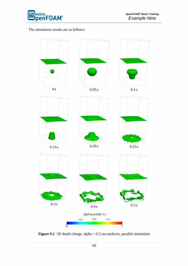
The simulation results are as follows:
0 s
0.05 s
0.1 s
0.15 s
0.20 s
0.25 s
0.3 s
0.4 s
0.5 s
Figure 9.1 3D depth charge, alpha = 0.5 iso-surfaces, parallel simulation
OpenFOAM
® Basic Training
Example Nine
51
Manual method
The manual method for decomposition is slightly different from the other three. In
order to use it:
Set the decomposeParDict file as any other simulation. For decomposition method,
choose either simple, hierarchical or scotch. Set the number of cores to the same
number which is going to be used for manual.
>decomposePar –cellDist
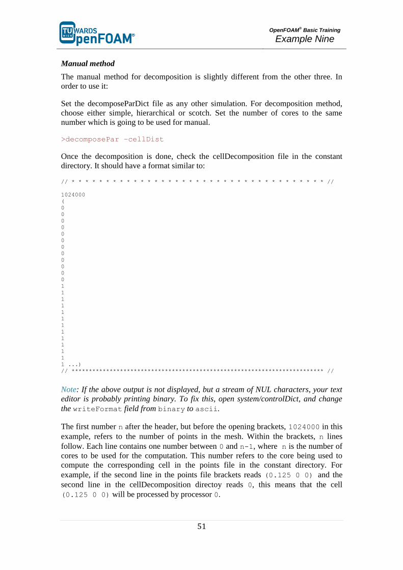
Once the decomposition is done, check the cellDecomposition file in the constant
directory. It should have a format similar to:
// * * * * * * * * * * * * * * * * * * * * * * * * * * * * * * * * * * * * * //
1024000
(
0
0
0
0
0
0
0
0
0
0
0
0
1
1
1
1
1
1
1
1
1
1
1
1
1 ...)
// ************************************************************************* //
Note: If the above output is not displayed, but a stream of NUL characters, your text
editor is probably printing binary. To fix this, open system/controlDict, and change
the writeFormat field from binary to ascii.
The first number n after the header, but before the opening brackets, 1024000 in this
example, refers to the number of points in the mesh. Within the brackets, n lines
follow. Each line contains one number between 0 and n-1, where n is the number of
cores to be used for the computation. This number refers to the core being used to
compute the corresponding cell in the points file in the constant directory. For
example, if the second line in the points file brackets reads (0.125 0 0) and the
second line in the cellDecomposition directoy reads 0, this means that the cell
(0.125 0 0) will be processed by processor 0.

OpenFOAM
® Basic Training
Example Nine
52
This cellDecomposition file can now be edited. Although this can be done manually,
it is probably not feasible for any sufficiently large mesh. The process must thus be
automated by writing a script to populate the cellDecomposition file according to the
desired processor breakdown.
When the new file is ready, save it under a different name:
>cp cellDecomposition manFile
Now, edit the decomposeParDict file. Select decomposition method manual, and for
the dataFile field in the manual coeffs range, specify the path to the file which
contains the manual decomposition. Note that OpenFOAM® searches in the constant
directory by default, in case relative paths are being used:
// * * * * * * * * * * * * * * * * * * * * * * * * * * * * * * * * * * * * * //
numberOfSubdomains 4;
method manual;
simpleCoeffs
{
n ( 1 4 1 );
delta 0.001;
}
hierarchicalCoeffs
{
n ( 1 4 1 );
delta 0.001;
order xyz;
}
manualCoeffs
{
dataFile "manFile";
}
distributed no;
roots ( );
// ************************************************************************* //
Run the simulation as usual.
Visualizing the processor breakdown
It may be interesting to visualize how exactly OpenFOAM® breaks down the mesh.
This can be easily visualized using ParaView. After running the simulation, but before
running the reconstructPar command, repeat the following for each of the processor
directories:
>cd processor<n>
where n is the processor number
>foamToVTK
convert the individual processor files to VTK, next, open ParaView:
OpenFOAM
® Basic Training
Example Nine
53
>paraview &
For each of the processor directories, perform the following steps:
- Open the VTK files in the relevant processor directory
- Double click them to open them and click on “Apply”
- The part of the mesh decomposed by that core will appear, in grey.
- Change the color in the drop-down menus in the toolbar. This is to ensure that each
individual part can be easily seen.
Once this is done for all processors, the entire mesh will appear. However, the
processor regions can now easily be seen in a different color.
In order to save this, there are two options. The first option is to take a screenshot:
File > Save a screenshot
The second option is to save the settings and modifications as a ParaView state file.
File > Save State
The current settings and modifications can then be easily recovered by:
File > Load State
Saving the state allows changes to be made afterwards. Saving a screenshot keeps
only a picture, while losing the ability to make changes after exiting ParaView. Doing
both is recommended.
OpenFOAM
® Basic Training
Example Ten
54
simpleFoam & scalarTransportFoam – TJunction
(Residence Time Distribution)
Simulation
Use the simpleFoam and scalarTransportFoam to simulate the flow through a square
cross section T pipe and calculate RTD (Residence Time Distribution) for both inlets
using a step function injection:
Inlet and outlet cross sections: 1 1 m2
Gas in the system: air at ambient conditions
Operating pressure: 105 Pa
Inlet 1: 0.1 m/s
Inlet 2: 0.2 m/s
Objectives
Understanding RTD calculation using OpenFOAM®
Using multiple solver for a simulation
Post processing
Plot the step response function and the RTD curve.
OpenFOAM
® Basic Training
Example Ten
55
Step by step simulation
Copy tutorial
Copy the following tutorial to your working directory as a base case:
~/OpenFOAM/OpenFOAM-2.3.0/tutorials/incompressible/simpleFoam
/pitzDaily
0 directory
Update p, U, nut, nuTilda, k and epsilon files with the new boundary conditions, e.g.
U:
// * * * * * * * * * * * * * * * * * * * * * * * * * * * * * * * * * * * * * //
dimensions [0 1 -1 0 0 0 0];
internalField uniform (0 0 0);
boundaryField
{
inlet_one
{
type fixedValue;
value uniform (0.1 0 0)
}
inlet_two
{
type fixedValue;
value uniform (-0.2 0 0)
}
outlet
{
type zeroGradient;
}
walls
{
type fixedValue;
value uniform (0 0 0)
}
}
// ************************************************************************* //
constant directory
Edit the blockMeshDict in the polyMesh directory as following for creating an
appropriate geometry.
// * * * * * * * * * * * * * * * * * * * * * * * * * * * * * * * * * * * * * //
convertToMeters 1.0;
vertices
(
(0 4 0) // 0
(0 3 0) // 1
(3 3 0) // 2
(3 0 0) // 3
(4 0 0) // 4
(4 3 0) // 5
(7 3 0) // 6
(7 4 0) // 7
(4 4 0) // 8
(3 4 0) // 9
(0 4 1) // 10

OpenFOAM
® Basic Training
Example Ten
56
(0 3 1) // 11
(3 3 1) // 12
(3 0 1) // 13
(4 0 1) // 14
(4 3 1) // 15
(7 3 1) // 16
(7 4 1) // 17
(4 4 1) // 18
(3 4 1) // 19
);
blocks
(
hex (0 1 2 9 10 11 12 19) (10 30 10) simpleGrading (1 1 1)
hex (9 2 5 8 19 12 15 18) (10 10 10) simpleGrading (1 1 1)
hex (8 5 6 7 18 15 16 17) (10 30 10) simpleGrading (1 1 1)
hex (2 3 4 5 12 13 14 15) (30 10 10) simpleGrading (1 1 1)
);
edges
(
);
patches
(
patch inlet_one
(
(0 10 11 1)
)
patch inlet_two
(
(7 6 16 17)
)
patch outlet
(
(4 3 13 14)
)
wall walls
(
(0 1 2 9)
(2 5 8 9)
(5 6 7 8)
(2 3 4 5)
(10 19 12 11)
(19 18 15 12)
(18 17 16 15)
(15 14 13 12)
(0 9 19 10)
(9 8 18 19)
(8 7 17 18)
(2 1 11 12)
(3 2 12 13)
(5 4 14 15)
(6 5 15 16)
)
);
mergePatchPairs
(
);
// ************************************************************************* //
Check RASProperties file for the turbulence model (kEpsilon).
// * * * * * * * * * * * * * * * * * * * * * * * * * * * * * * * * * * * * * //
RASModel kEpsilon;
turbulence on;
printCoeffs on;
// ************************************************************************* //
OpenFOAM
® Basic Training
Example Ten
57
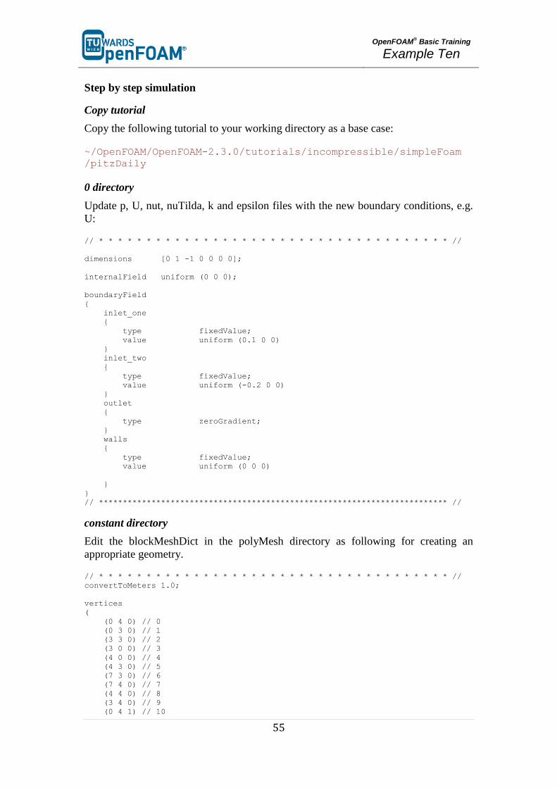
Running simulation
>blockMesh
Figure 10.1 mesh created using blockMesh
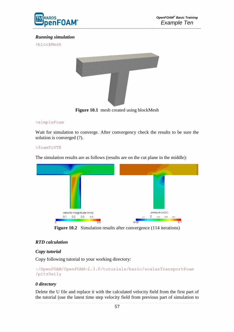
>simpleFoam
Wait for simulation to converge. After convergency check the results to be sure the
solution is converged (?).
>foamToVTK
The simulation results are as follows (results are on the cut plane in the middle):
Figure 10.2 Simulation results after convergence (114 iterations)
RTD calculation
Copy tutorial
Copy following tutorial to your working directory:
~/OpenFOAM/OpenFOAM-2.3.0/tutorials/basic/scalarTransportFoam
/pitzDaily
0 directory
Delete the U file and replace it with the calculated velocity field from the first part of
the tutorial (use the latest time step velocity field from previous part of simulation to
OpenFOAM
® Basic Training
Example Ten
58
calculate RTD for this geometry). There is no need to modify or change it. The solver
will use this field to calculate the scalar transportation.
Update T (T will be used as an inert scalar in this simulation) file boundary conditions
to match new simulation boundaries, to calculate RTD of the inlet_one set the
internalField value to 0, T value for inlet_one to 1.0 and T value for
inlet_two to 0.
constant directory
Replace the blockMeshDict file with the one from the first part of tutorial.
system directory
In the controlDict file change the endTime from 0.1 to 120 (approximately two
times ideal resistance time) and also deltaT from 0.0001 to 0.1 (Courant number
approximately 0.4).
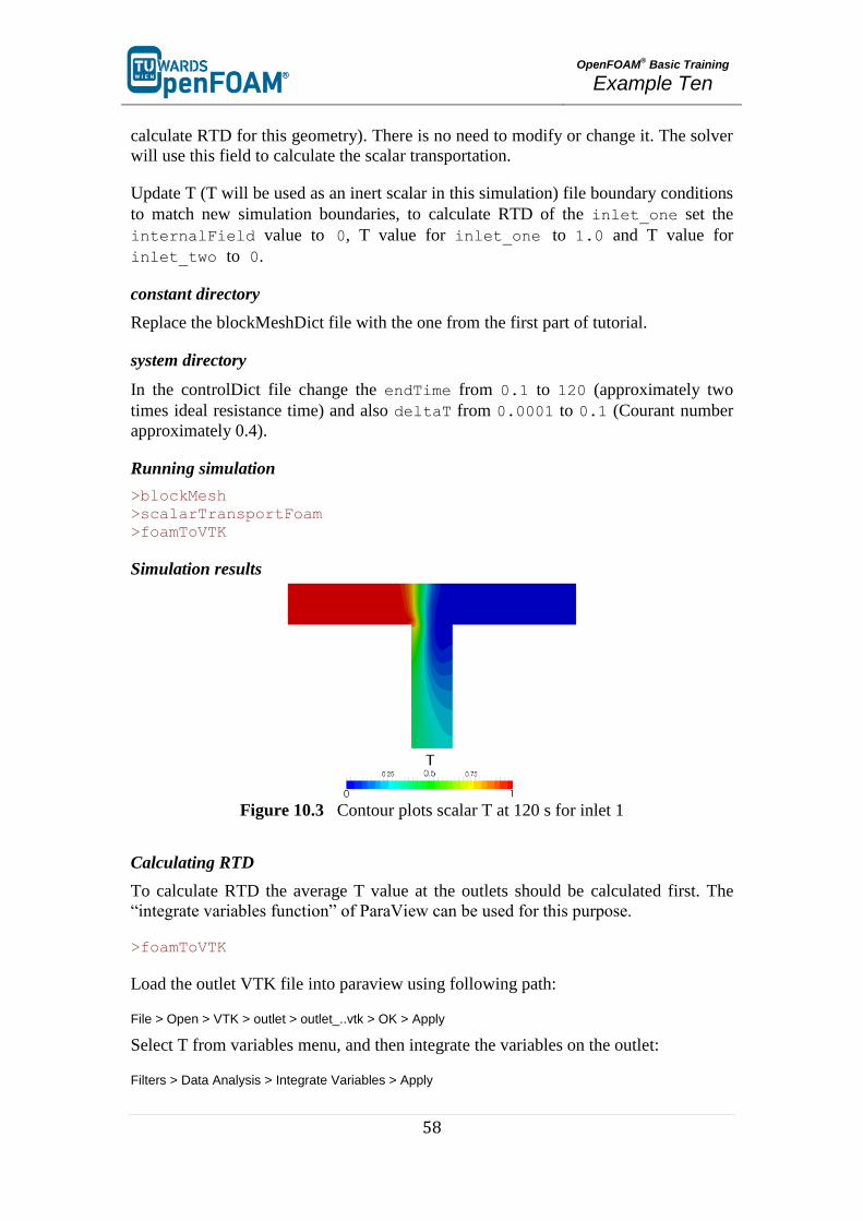
Running simulation
>blockMesh
>scalarTransportFoam
>foamToVTK
Simulation results
Figure 10.3 Contour plots scalar T at 120 s for inlet 1
Calculating RTD
To calculate RTD the average T value at the outlets should be calculated first. The
“integrate variables function” of ParaView can be used for this purpose.
>foamToVTK
Load the outlet VTK file into paraview using following path:
File > Open > VTK > outlet > outlet_..vtk > OK > Apply
Select T from variables menu, and then integrate the variables on the outlet:
Filters > Data Analysis > Integrate Variables > Apply
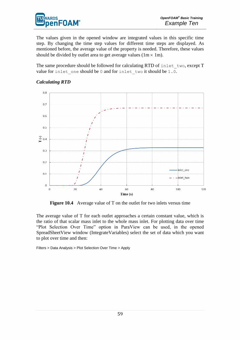
OpenFOAM
® Basic Training
Example Ten
59
The values given in the opened window are integrated values in this specific time
step. By changing the time step values for different time steps are displayed. As
mentioned before, the average value of the property is needed. Therefore, these values
should be divided by outlet area to get average values (1m 1m).
The same procedure should be followed for calculating RTD of inlet_two, except T
value for inlet_one should be 0 and for inlet_two it should be 1.0.
Calculating RTD
Figure 10.4 Average value of T on the outlet for two inlets versus time
The average value of T for each outlet approaches a certain constant value, which is
the ratio of that scalar mass inlet to the whole mass inlet. For plotting data over time
“Plot Selection Over Time” option in ParaView can be used, in the opened
SpreadSheetView window (IntegrateVariables) select the set of data which you want
to plot over time and then:
Filters > Data Analysis > Plot Selection Over Time > Apply
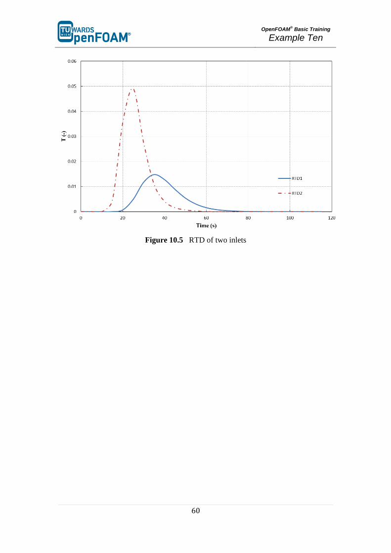
OpenFOAM
® Basic Training
Example Ten
60
Figure 10.5 RTD of two inlets
OpenFOAM
® Basic Training
Example Eleven
61
reactingFoam – reactingElbow
Simulation
Use the reactingFoam solver, simulate combustion of CH4 and O2 in a mixing elbow:
Use the two times finer Hex mesh from Example One
Domain initially filled with N2
velocity-inlet-5:
- Velocity: 1 m/s
- Mass fractions: 23 % O2, 77 % N2
- Temperature: 800 K
velocity-inlet-6:
- Velocity: 3 m/s
- Mass fractions: 50 % CH4, 50 % N2
- Temperature: 293 K
Operating pressure: 105 Pa
Operating temperature: 298 K
Isolated walls
Objective
Understanding multi-species and reaction modeling in OpenFOAM®
Post processing
Evaluate your results in ParaView.
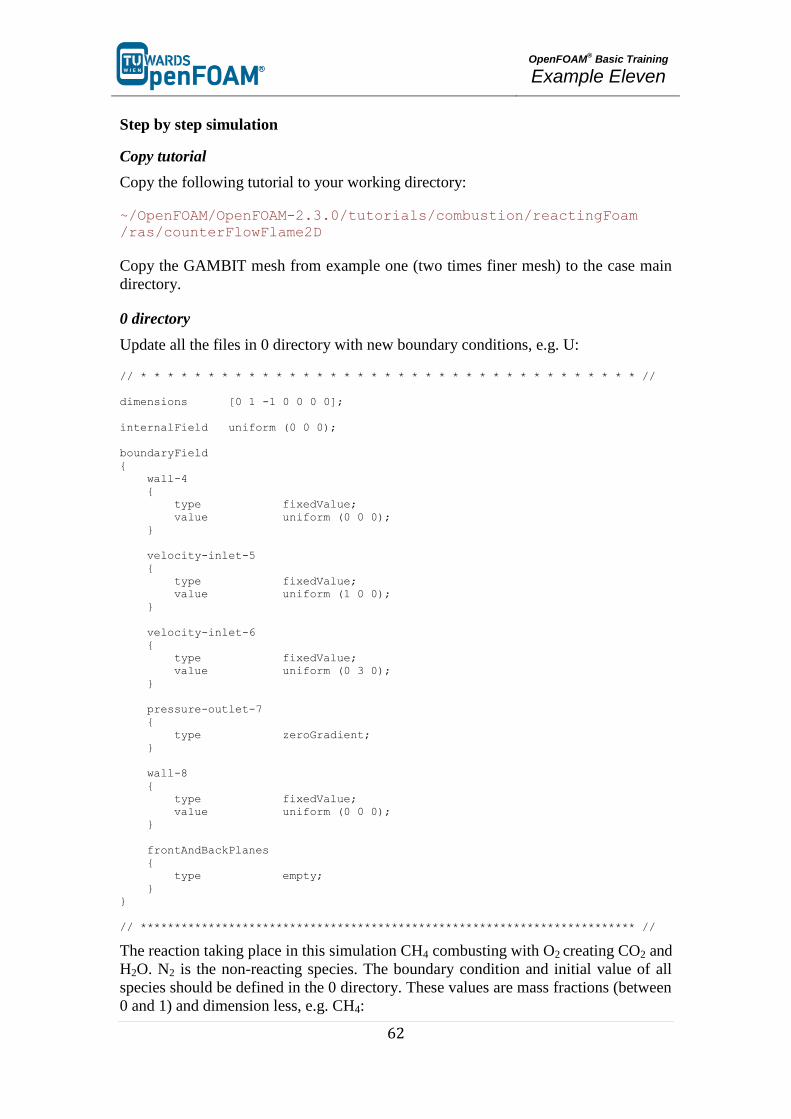
OpenFOAM
® Basic Training
Example Eleven
62
Step by step simulation
Copy tutorial
Copy the following tutorial to your working directory:
~/OpenFOAM/OpenFOAM-2.3.0/tutorials/combustion/reactingFoam
/ras/counterFlowFlame2D
Copy the GAMBIT mesh from example one (two times finer mesh) to the case main
directory.
0 directory
Update all the files in 0 directory with new boundary conditions, e.g. U:
// * * * * * * * * * * * * * * * * * * * * * * * * * * * * * * * * * * * * * //
dimensions [0 1 -1 0 0 0 0];
internalField uniform (0 0 0);
boundaryField
{
wall-4
{
type fixedValue;
value uniform (0 0 0);
}
velocity-inlet-5
{
type fixedValue;
value uniform (1 0 0);
}
velocity-inlet-6
{
type fixedValue;
value uniform (0 3 0);
}
pressure-outlet-7
{
type zeroGradient;
}
wall-8
{
type fixedValue;
value uniform (0 0 0);
}
frontAndBackPlanes
{
type empty;
}
}
// ************************************************************************* //
The reaction taking place in this simulation CH4 combusting with O2 creating CO2 and
H2O. N2 is the non-reacting species. The boundary condition and initial value of all
species should be defined in the 0 directory. These values are mass fractions (between
0 and 1) and dimension less, e.g. CH4:
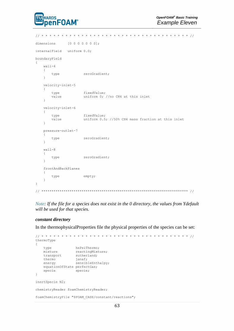
OpenFOAM
® Basic Training
Example Eleven
63
// * * * * * * * * * * * * * * * * * * * * * * * * * * * * * * * * * * * * * //
dimensions [0 0 0 0 0 0 0];
internalField uniform 0.0;
boundaryField
{
wall-4
{
type zeroGradient;
}
velocity-inlet-5
{
type fixedValue;
value uniform 0; //no CH4 at this inlet
}
velocity-inlet-6
{
type fixedValue;
value uniform 0.5; //50% CH4 mass fraction at this inlet
}
pressure-outlet-7
{
type zeroGradient;
}
wall-8
{
type zeroGradient;
}
frontAndBackPlanes
{
type empty;
}
}
// ************************************************************************* //
Note: If the file for a species does not exist in the 0 directory, the values from Ydefault
will be used for that species.
constant directory
In the thermophysicalProperties file the physical properties of the species can be set:
// * * * * * * * * * * * * * * * * * * * * * * * * * * * * * * * * * * * * * //
thermoType
{
type hePsiThermo;
mixture reactingMixture;
transport sutherland;
thermo janaf;
energy sensibleEnthalpy;
equationOfState perfectGas;
specie specie;
}
inertSpecie N2;
chemistryReader foamChemistryReader;
foamChemistryFile "$FOAM_CASE/constant/reactions";
OpenFOAM
® Basic Training
Example Eleven
64
foamChemistryThermoFile "$FOAM_CASE/constant/thermo.compressibleGas";
// ************************************************************************* //
The mixture type is set to a reacting mixture for calculating the mixture properties and
the heat capacities are calculated using “janaf polynomials”.
N2 is defines as inertSpecie. In reaction solvers in OpenFOAM® the inert specie is
calculated explicitly using the mass balance equation (to satisfy mass conservation):
∑
The species and the reactions are addressed using foamChemistryFile. In this
simulation reactions and species are read from reactions file in the constant directory:
species
(
O2
H2O
CH4
CO2
N2
);
reactions
{
methaneReaction
{
type irreversibleArrheniusReaction;
reaction "CH4 + 2O2 = CO2 + 2H2O";
A 5.2e16;
beta 0;
Ta 14906;
}
}
The species in this simulation are O2, H2O, CH4, CO2 and N2. They are defined in the
species sub-dictionary. In the reactions sub-dictionary, reactions are specified.
The reaction of methane combustion is defined and it is of type irreversible
Arrhenius reaction, irreversibleArrheniusReaction.
In the Example Two it was explained the coefficients for calculating gas mixture
properties are defined in the mixture sub-dictionary because it was a homogeneous
mixture. But in this example the mixture is not homogenous so coefficients for
calculating properties of each species are needed separately to calculate mixture
properties based on each cell composition. The coefficients of each species are
defined in the foamChemistryThermoFile, which reads the file
thermo.compressibleGas from the constant directory, e.g. for O2 coefficients for each
model is mentioned bellow:
// * * * * * * * * * * * * * * * * * * * * * * * * * * * * * * * * * * * * * //
O2
{
specie
{
nMoles 1;
molWeight 31.9988;
}
thermodynamics
OpenFOAM
® Basic Training
Example Eleven
65
{
Tlow 200;
Thigh 5000;
Tcommon 1000;
highCpCoeffs ( 3.69758 0.00061352 -1.25884e-07 1.77528e-11 -
1.13644e-15 -1233.93 3.18917 );
lowCpCoeffs ( 3.21294 0.00112749 -5.75615e-07 1.31388e-09 –
8.76855e-13 -1005.25 6.03474 );
}
transport
{
As 1.67212e-06;
Ts 170.672;
}
}
…
// ************************************************************************* //
In the thermodynamics sub-dictionary the janaf polynomial model coefficients for
calculating the heat capacity can be found and in transport the sutherland model
coefficients for viscosity are stored.
system directory
By setting the adjustTimeStep to yes in the controlDict, the solver automatically
ignores deltaT, and calculates the deltaT based on the maximum Courant number
maxCo defined for it. Change the endTime to 120 (approximately one time the
volumetric residence time based on velocity-inlet-5) and writeTimeInterval to
10, to write every 10 s to case directory.
// * * * * * * * * * * * * * * * * * * * * * * * * * * * * * * * * * * * * * //
application reactingFoam;
startFrom startTime;
startTime 0;
stopAt endTime;
endTime 120;
deltaT 1e-6;
writeControl adjustableRunTime;
writeInterval 10;
purgeWrite 0;
writeFormat ascii;
writePrecision 6;
writeCompression off;
timeFormat general;
timePrecision 6;
runTimeModifiable true;
adjustTimeStep yes;
maxCo 0.4;

OpenFOAM
® Basic Training
Example Eleven
66
// ************************************************************************* //
Running simulation
>fluentMeshToFoam fineHex.msh
After converting the mesh, check the boundary file in the constant/polyMesh directory
and change the type and inGroups of boundary frontAndBackPlanes from
wall to empty (it is a 2D simulation).
>reactingFoam
>foamToVTK
The simulation results are as follows:
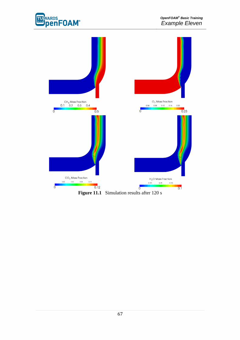
OpenFOAM
® Basic Training
Example Eleven
67
Figure 11.1 Simulation results after 120 s

OpenFOAM
® Basic Training
Appendix A
68
Appendix A
Important commands in Linux Terminals
(Mostly on Unix [IRIX, Alpha Unix… usable])
cat, more, less
File viewer with pure read function - in order of ease of operation. In
less with pagedown/pageup you can navigate within the file, with / and
? can forward / backward search for strings, q can be used for closing
less. cat is universally available on Unix.
cd, cd ..
Changing the directory, cd .. goes one directory up and cd ~ moves to
home directory. Important to note is the space between cd and .. as
opposed to DOS!
cp, cp -r
Copying files or entire directory trees (with -r option). Caution: There is
no warning or prompt when overwriting existing files! The important
thing is that a target has to be always given, at least one . which means,
copy to the current directory.
ctrl+r Reverse command line search, for searching an already typed command
in a terminal window.
du, du -s,
du -k
Calculates the amount of space consumed in a directory. For safety
reasons you should use the -k option (output in kilobytes), since some
systems provide the space in blocks that include only 512 bytes ...
exit Closing connection (terminal window).
gedit Text editor with graphical user interface. When working with gedit
some temporary files (originalFileName~) are created, they can be
deleted after saving.
grep Search command for plain-text data sets for lines matching a regular
expression.
gzip, gunzip
Compression/decompression program for individual files (as opposed to
zip/unzip, this can also work on directories or file lists). The great
advantage of gzip: Fluent® and OpenFOAM
® are able to read and write
gz files directly, which saves about 30-90% space.
kill, kill -9 Stopping processes. For this the process ID is required, which can be
OpenFOAM
® Basic Training
Appendix A
69
found with top or ps. The Exit is irrevocable course - but you cannot
shoot processes, if you are not the "owner".
ls, ls –la
Lists the contents of a directory, with option -la also hidden files are
displayed, as well as the file size and characteristics.
mc Program that enables navigation in the text window, esc-keys, may be
necessary: mc -c, for navigating through mc use function keys or
esc+[number] combination, e.g. F9 or esc+9 for moving to the menus at
the top.
mkdir
Creates a new directory.
mv Moving or renaming files and directories. Caution: There is no prompt
when overwriting existing files!
nano, pico The command to run the nano text editor, a terminal based text editor.
passwd
The command to change the login password.
| It is known as pipe and is used for merging two commands, redirecting
one command as input to another, e.g. less|grep searches a specified
word in the output of file opened with less.
ps, ps –A
ps waux
Lists all the processes that were started in the respective command
window with the options are all running processes on the system
display.
pwd
Shows the current working directory.
rm,
CAUTION:
rm -fr
Deletes files. The option -r will also remove directories and files
recursively and delete directories, f (force) prevents any further inquiry.
- Incorrectly applied, this command can lead to irreversible loss of all
(private) data. There is no undelete or undo!
rmdir
Deletes an empty directory.
scp
The copy command over the network - as secure FTP replacement. Also
dominates the -r (recursive) option. Usage: scp source file destination
file with source and the destination format can be USERNAME@

OpenFOAM
® Basic Training
Appendix A
70
COMPUTER.DOMAIN:PATH/TO/FILE. Source or target can of course
also be created locally, then (your) user name and computer are not
required.
ssh
Telnet replacement with encryption used to connect to remote machines.
On Windows, for example, implemented with putty.
tail, tail -f
File viewer, the default outputs the last 10 lines of a file. With option -
n XX can spend the last XX lines, with the -f option, the command is
running from those lines, which are attached to a file. The command is
therefore perfect for watching log files.
top Displays a constantly updated list of all running processes, with process
ID, memory and CPU usage. For processes of one user top [username]
should be used, and for quitting q or ctrl+c should be applied.
vi, vim File editor. For forward searching use /, for backward searching use ?.
For exiting esc+:x. nano or pico are recommended for beginners, which
are easier to handle.
OpenFOAM
® Basic Training
Appendix B
71
Appendix B
Running OpenFOAM®
Part A) Running OpenFOAM® on a Local Linux PC (or virtual machine):
Open a terminal
Go to the OpenFOAM®
installation directory (e.g. /opt/openfoam230) in the
opened terminal
Change to the etc directory in the OpenFOAM® installation directory
Run the following command:
>. ./bashrc
If a new terminal is opened, the same procedure should be repeated in that in
order to activate OpenFOAM® in here.
Part B) Running OpenFOAM® on Remote Computers via SSH (e.g. server):
B-1) Windows:
Run PuTTY (search for: PuTTY windows).
Set the following:
Category>Session
Host name: openhost.university.edu
Connection type: SSH
Category>Connection>SSH>Tunnels
Source port: 5901
Destination: localhost:59**1
Do not forget to press Add!
Please make sure that this display is not used by others.
Category>Connection>Data
Auto-login username: openFoamUser
Category>Session
1 Display number

OpenFOAM
® Basic Training
Appendix B
72
Saved Sessions: openFoamUser
Press Save.
Now choose from “saved sessions” your session (openFoamUser) and press
Open. In the opened Command (Prompt) window, it prompts for your
password. The password is not echoed to the screen and the passwords are
case sensitive.
Immediately after entering your password, your computer will attempt to
establish a connection to your server. If it is your first time connecting to that
server, you will see a message asking you to confirm the identity of the
machine. Make sure you entered the address properly, and type yes, followed
by the return key, to proceed.
To log out use whatever command is used to logout from the server you are
logged into (typically exit / ctrl + d).
B-2) Mac OS X and Linux:
Open your Terminal application. You will see a window with a $ or > symbol
and a blinking cursor. From here, you may issue the following command to
establish the SSH connection to your server (be careful about upper case „L‟ in
the -gL).
>ssh -gL 5901:localhost:59** [email protected]
Immediately after issuing this command, your computer will attempt to
establish a connection to your server. If it is your first time connecting to that
server, you will see a message asking you to confirm the identity of the
machine. Make sure you have entered the address properly, and type yes,
followed by the return key, to proceed.
You will then be prompted to enter your password. Type or copy/paste your
SSH user password into the Terminal. You will not see the cursor moving
while entering your password. This is normal. Once you are finished inputting
your password, press return on your keyboard. At this point, you will be
connected to your server remotely through SSH.
Part C) Running OpenFOAM® in Graphical Interface (VNC):
Connect to remote machine via SSH connection using part B.
Make sure VNC Server is installed on the remote machine and it is started (ask
administrator for display number, port and other information, for starting
VNC Server check FAQ)
Install the appropriate VNC Viewer and run it (search for: vnc viewer):
VNC Server: localhost:01
OpenFOAM
® Basic Training
Appendix B
73
Press Connect
Press Continue
Enter your password
Press Ok
On VNC desktop open a terminal
Change to etc directory in OpenFOAM®
installation directory
Execute the following command:
>. ./bashrc
If a new terminal in the VNC desktop is opened, the last two steps should be
done in that to activate OpenFOAM® in there (or add to bashrc).
OpenFOAM
® Basic Training
Appendix C
74
Appendix C
Frequently Asked Questions (FAQ)
Q - What should I do in case of a GAMBIT failure?
A - e.g. Program stops responding:
Type "ps" in the command window, search for the GAMBIT process number.
"kill -9 PROCESS NUMBER" Enter
GAMBIT creates lock files, which must also be deleted, otherwise it is not
possible to open of the affected files:
"rm *. lok" Enter
Furthermore, "junk" (temporary files from GAMBIT) should be disposed of:
"rm -fr GAMBIT.xxx" erases the complete directory, xxx again is the
process number.
If you have forgotten to save before the crash, you should copy the file "jou"
(it contains all the commands that have been executed and can be processed
automatically in GAMBIT) from the directory, to resume its status before
the crash.
Q - How can I prevent typing long commands in the terminal for couple of times?
A - Using curser keys to navigate line by line.
Type beginning of the command and use Tab (auto completion).
By using reverse search, use ctrl+r to search for previous commands typed in
the terminal, e.g. typing a part of command show the suggestions and you can
navigate through them.
Q - My VNC is not responding from server side?
A - First you should kill your VNC server:
>vncserver –kill :[YOUR DISPLAY NUMBER]
Restart your VNC server (according to SSH forward):
>vncserver:[YOUR DISPLAY NUMBER] -geometry 1600x800 -depth
24
Q - I have deleted some of my files accidently. What should I do?
A - Sorry, no recycling or undelete in Linux
Q - Why can I not connect to the server?
A - Check to see if you have an IP address for your network card.
Q - How can I start VNC Viewer from my Linux computer terminal?
A - Use command:
OpenFOAM
® Basic Training
Appendix C
75
>vncviewer :[NUMBER OF LOCAL PORT, e.g. 1 or 2]
Q - Error “command not found”?
A - Make sure OpenFOAM®
and ParaView are installed correctly. Check Appendix
B for starting OpenFOAM®.
Q - Does foamToVTK command not work for chtMultiRegionFoam?
A - Use command:
>foamToVTK –region[REGION NAME]
Q - Is it possible to export animations from ParaView?
A - Yes, by choosing .ogv file format from “file/save animation” menu. The output
will be a video file with .ogv format. In the new ParaView versions (4.3.0) the
animation can also be saved using .avi format.
Q - Is there any tool in Linux to convert series of ParaView pictures to video?
A - Yes, command line tool ffmpeg:
>ffmpeg –r [FRAME PER SECOND RATE] –f image2 –i [images
names, e.g. rho.%4d.jpg] [OUTPUT FILE NAME].[OUTPUT FILE
FORMAT, e.g avi]
Q - How can complex geometries be patched?
A - During creating the geometry in the preprocessing software, e.g. GAMBIT,
create volume zones, which you will need to patch later (see software user
manual for creating regions in each software). For converting the mesh to the
OpenFOAM® mesh use the appropriate tool with “-writeZones” flag to import
zones to OpenFOAM®, e.g.:
>fluentMeshToFoam -writeZones <your mesh>
then in the setFieldDict change it like this:
regions
(
zoneToCell
{
name air; // region name which you assigned in gambit
fieldValues
(
volScalarFieldValue alpha.water 0 // the value of property
//which you want to patch
);
}
);
Then after running setFields tool, it will assign the values to that region.
Q - How can I create a bash scripting file for executing couple of command in
series?
A - Instead of typing command sequences one by one after each other and executing
OpenFOAM
® Basic Training
Appendix C
76
them. It is possible to put all those commands in a file and execute that file to
run them. This is known as “bash scripting”.
Bash scripting is typically used in the cases when the same simulation should be
run with identical settings a couple of times, but with a few changes. For bash
scripting create an empty file (e.g. using nano editor creating text file “go”):
> nano go
Add the commands to this file (e.g. commands for running blockMesh,
setFields, decomposePar, compressibleInterFoam in parallel mode and
reconstructPar):
blockMesh
setFields
decomposePar
mpirun –np 4 compressibleInterFoam –parallel >log
reconstructPar
Exit the editor and save the file (ctrl+x , y, enter for nano editor).
For changing this file to an executable file, file permissions should be set. By
using this command file permissions are displayed:
>ls –la go
-rw-r--r-- 1 e166**** E020D166 73 Aug 23 9:15 go
The first „r‟ shows that this text file can be read by user, the „w‟ shows that user
has the permission to write this file, but the „–„ sign shows that this file is not
executable by the user. To change this permissions execute following command:
>chmod u+x go
Now this file is executable:
>ls –la go
-rwxr--r-- 1 e166**** E020D166 73 Aug 23 9:15 go
Now you can run the simulation by this executable text file:
>./go
After executing the file, the commands added to the file will be executed one by
one. In most of the OpenFOAM® tutorials there are Allrun and Allclean files,
which are bash scripts for running the case and cleaning a case, respectively.
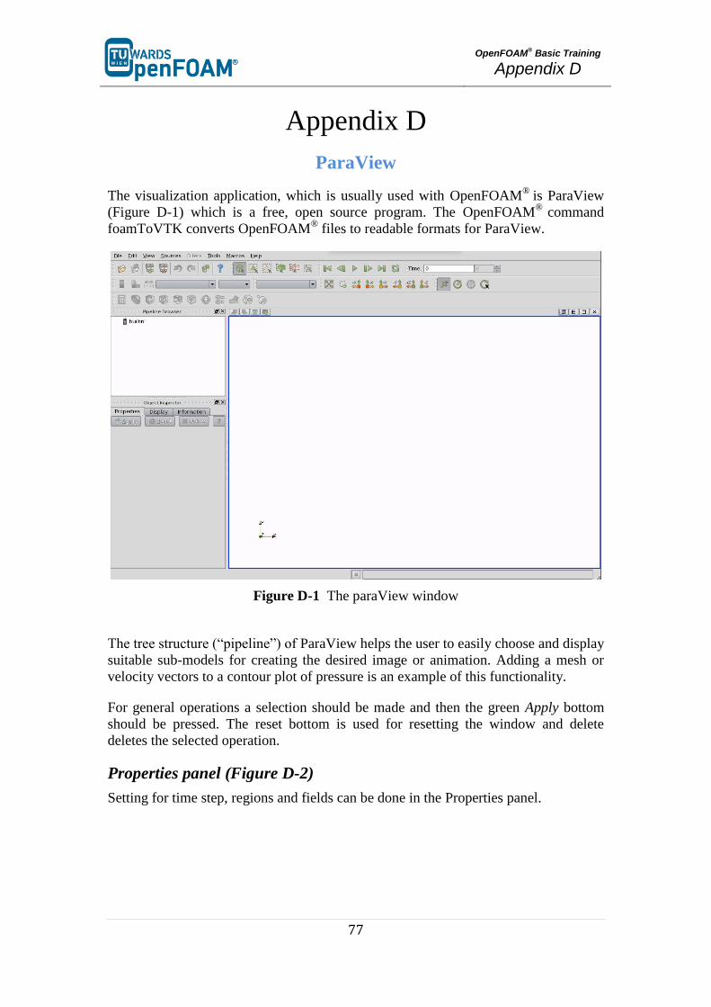
OpenFOAM
® Basic Training
Appendix D
77
Appendix D
ParaView
The visualization application, which is usually used with OpenFOAM®
is ParaView
(Figure D-1) which is a free, open source program. The OpenFOAM®
command
foamToVTK converts OpenFOAM® files to readable formats for ParaView.
Figure D-1 The paraView window
The tree structure (“pipeline”) of ParaView helps the user to easily choose and display
suitable sub-models for creating the desired image or animation. Adding a mesh or
velocity vectors to a contour plot of pressure is an example of this functionality.
For general operations a selection should be made and then the green Apply bottom
should be pressed. The reset bottom is used for resetting the window and delete
deletes the selected operation.
Properties panel (Figure D-2)
Setting for time step, regions and fields can be done in the Properties panel.
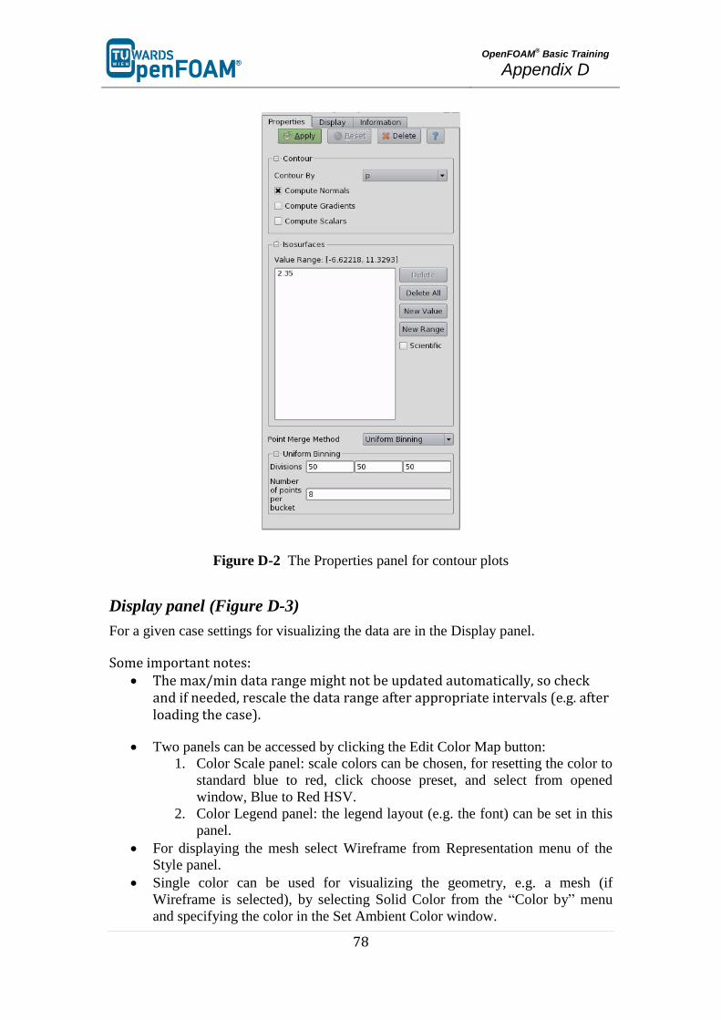
OpenFOAM
® Basic Training
Appendix D
78
Figure D-2 The Properties panel for contour plots
Display panel (Figure D-3)
For a given case settings for visualizing the data are in the Display panel.
Some important notes: The max/min data range might not be updated automatically, so check
and if needed, rescale the data range after appropriate intervals (e.g. after loading the case).
Two panels can be accessed by clicking the Edit Color Map button:
1. Color Scale panel: scale colors can be chosen, for resetting the color to
standard blue to red, click choose preset, and select from opened
window, Blue to Red HSV.
2. Color Legend panel: the legend layout (e.g. the font) can be set in this
panel.
For displaying the mesh select Wireframe from Representation menu of the
Style panel.
Single color can be used for visualizing the geometry, e.g. a mesh (if
Wireframe is selected), by selecting Solid Color from the “Color by” menu
and specifying the color in the Set Ambient Color window.

OpenFOAM
® Basic Training
Appendix D
79
The opacity of the image can be set (1 = solid, 0 = invisible) in the Opacity in
the Style panel.
Figure D-3 The Display panel
Button toolbars
Pull-down menus at the top of the main window and the major panels, in the toolbars
below the main pull-down menus increase the functionality of ParaView. The
function of each button can be easily understood by its icon (Figure D-4), also any
button description can be found in the Help menu (keeping the mouse over an icon
without clicking on it will also give a short explanation on its functionality).
Figure D-4 Toolbars in ParaView

OpenFOAM
® Basic Training
Appendix D
80
Manipulating the view
View settings
The View menu from Edit menu contains three items: General, Lights and
Annotation.
The General panel includes the following items (which are often set at startup):
The background color, from arrow down Choose Color button.
Parallel projection is the usual choice for 2D, CFD simulations.
The lighting controls are in Lights panel in the Light Kit panel. For producing images
with strong bright colors (e.g. isosurface) Headlight of strength 1 is appropriate.
For including annotations in the image Annotation panel should be used. The
Orientation Axes feature controls an axes icon in the image window (e.g. to set the
color of the axes labels x, y and z).
General settings
Some default behavior of ParaView can be controlled in the General panel. The Auto
Accept button enables accepting the changes without pressing the Apply button (not a
very good option for big cases because re-rendering the image after each change takes
a long time)
The Render View panel contains three sub-items: General, Camera and Server. The
level of detail (LOD) is included in the General panel which controls the rendering of
the image while it is being manipulated (e.g. rotated or resized); lower levels allow
cases with large numbers of cells to be re-rendered quickly during manipulation.
The Camera panel includes control settings for 3D and 2D movements. The user can
edit the rotation, translation and the zoom map to make it suitable for these needs.
This can be used by a combination of mouse, Shift and Control keys.
Contour plots
Selecting Contour from the Filter menu at the top menu bar creates a contour plot.
If the case is a 3D case module, the contours will be a set of 2D surfaces that
represent a constant value. There is Isosurface list in the Properties panel that the
users can edit by New Range window in the most convenient way. The chosen scalar
field is selected from a pull down menu.
Introducing a cutting plane
Creating contour plots across a plane is more convenient than isosurfaces. Cutting
planes are the tools which can be used for this purpose, to create surfaces. This can be
done by Slice filters, using cutting Plane, Box or Sphere options. A cutting plate can
be manipulated like other by mouse. In a similar way, the contour lines can also be
derived out of planes.
OpenFOAM
® Basic Training
Appendix D
81
By default ParaView triangulate the cells and shows them as triangles. For disabling
this uncheck “triangulate the slice” option in the properties window of slice.
Vector plots
The Glyph filter is used for creating vector plots. Scale Mode menu in the properties
panel is used for:
- Setting the length of a vector, weather to be proportional to vector magnitude
or not, all with the same length (Vector).
- Controlling the base length of the glyphs (set Scale Factor).
Plotting at cell centers
Vectors at cell centers are more common, for this purpose the Cell Centers filter
should be applied before Glyph filter.
Streamlines
Creating tracer lines, using the Stream Tracer filter create streamlines. Tracer points
can be along a line or point which are shown in white, and can be choose from Tracer
Seed panel. Usually, some trial and error is needed for achieving the desired
streamlines, the length of steps tracer takes can be changed in the main Stream Tracer
panel, a smaller length increase calculation time but increase smoothness. For having
high quality images Tubes filter can be used after tracer lines have been created.
There are different types of tubes, not only cylindrical.
Image output
For creating a screenshot of the graphs the easiest way is Save Screenshot from File
menu. After selecting it in the opened window the picture resolution can be set, and
by locking the aspect ratio, changing image resolution in one direction cause change
in its resolution in the other direction respectively. For high quality images a
resolution of more than 1000 pixels is a good choice.
Animation output
Some animations can be also created using ParaView in the File menu by choosing
animation and setting the resolution, and also frames per time step. You can save your
animation by assigning a name and choosing file format, and then the captured
pictures are saved with this format:
“<fileRoot>_<imageNo>.<fileExt>”
In the newer versions of ParaView (4.3.1), it is possible to export directly as
animation with .ogv or avi format. Do the same as before, except in the saving
window select .ogv or .avi for file format.
Top Related