


Languages
Pages
Legal

Numerical Solution of ODE IVPs�
L.G. de Pillis and A.E. Radunskaya
July 30, 2002
�This work was supported in part by a grant from the W.M. Keck Foundation
0-0
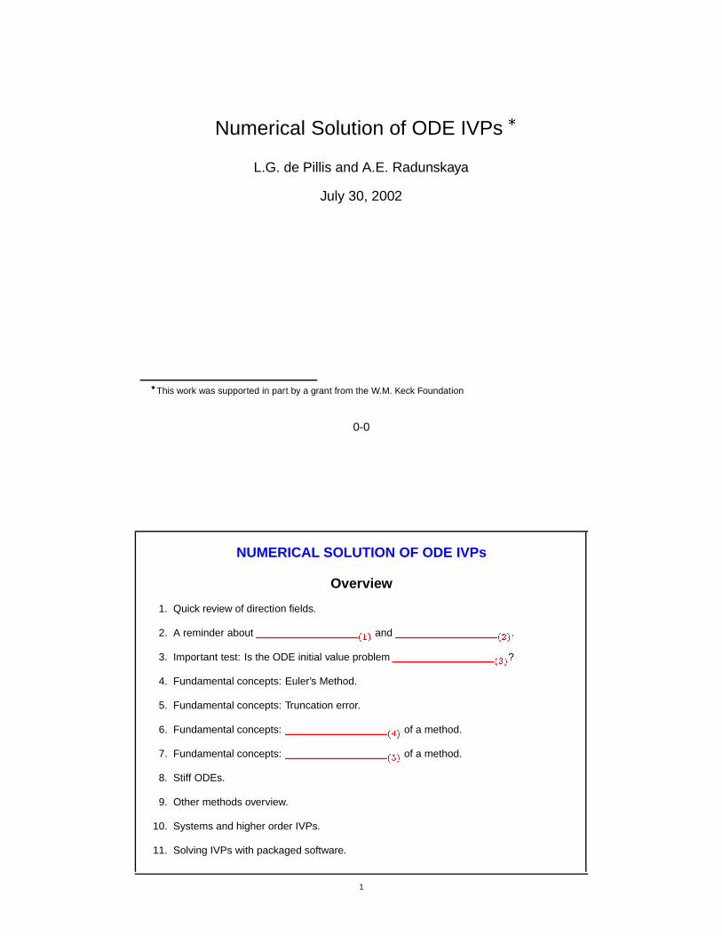
NUMERICAL SOLUTION OF ODE IVPs
Overview
1. Quick review of direction fields.
2. A reminder about ����� and ���� .
3. Important test: Is the ODE initial value problem ���� ?
4. Fundamental concepts: Euler’s Method.
5. Fundamental concepts: Truncation error.
6. Fundamental concepts: � ��� of a method.
7. Fundamental concepts: ���� of a method.
8. Stiff ODEs.
9. Other methods overview.
10. Systems and higher order IVPs.
11. Solving IVPs with packaged software.
1

Numerical Solution of ODE IVPs
Notes for Overview slide:
Answers:
(1) existence
(2) uniqueness
(3) well-posed
(4) Order
(5) Stability
We are assuming the students have had an introductory course in ordinary differen-
tial equations, so they have seen direction fields and existence and uniqueness theory
before. Direction fields are re-introduced to the students because they provide a natural
lead-in to the geometric derivation of Euler’s method. As you discuss the items on the
Overview list, you may want to keep in mind the following:
� Euler’s method is introduced for illustration only. It is a good pedagogical device
for giving understanding about how numerical ODE solvers work fundamentally,
1-1
but it is a method that nobody should use in practice. There are far better meth-
ods available for use.
� Euler’s method is an example of an “explicit” “single-step” method.
� When we introduce other methods, we will not get into any details at all, since
those can be learned in a course on numerical analysis. We will simply give an
overview of the categories of solvers available.
1-2
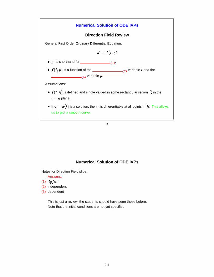
Numerical Solution of ODE IVPs
Direction Field Review
General First Order Ordinary Differential Equation:
����������� ������ � is shorthand for ����� .������� ��� is a function of the ��� � variable and the
����� variable � .Assumptions:
������� ��� is defined and single valued in some rectangular region � in the���� plane.
� If ��� �!�"� is a solution, then it is differentiable at all points in � . This allows
us to plot a smooth curve.
2
Numerical Solution of ODE IVPs
Notes for Direction Field slide:
Answers:
(1) # ��$ # (2) independent
(3) dependent
This is just a review, the students should have seen these before.
Note that the initial conditions are not yet specified.
2-1
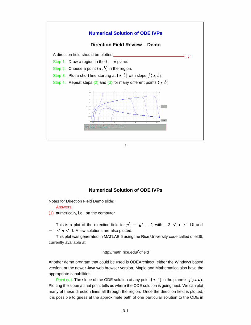
Numerical Solution of ODE IVPs
Direction Field Review – Demo
A direction field should be plotted ����� .Step 1: Draw a region in the � � plane.
Step 2: Choose a point ��� ��� � in the region.
Step 3: Plot a short line starting at ������� � with slope ��������� � .Step 4: Repeat steps (2) and (3) for many different points ������� � .
−2 0 2 4 6 8 10
−4
−3
−2
−1
0
1
2
3
4
t
y
y ’ = y2 − t
3
Numerical Solution of ODE IVPs
Notes for Direction Field Demo slide:
Answers:
(1) numerically, i.e., on the computer
This is a plot of the direction field for �������� �� , with �������� ��� and
���������� . A few solutions are also plotted.
This plot was generated in MATLAB 6 using the Rice University code called dfield6,
currently available at
http://math.rice.edu/� dfield
Another demo program that could be used is ODEArchitect, either the Windows based
version, or the newer Java web browser version. Maple and Mathematica also have the
appropriate capabilities.
Point out: The slope of the ODE solution at any point �! #"�$&% in the plane is '(�! #"�$&% .Plotting the slope at that point tells us where the ODE solution is going next. We can plot
many of these direction lines all through the region. Once the direction field is plotted,
it is possible to guess at the approximate path of one particular solution to the ODE in
3-1
the family of solutions, since any solution is tangent to these direction field lines. Any
single solution is then specified by a point that it goes through.
As a preview, the following questions could be asked:
1. Given a point ������� � � is there always a solution through that point tangent to the
direction field? If the direction field is “vertical”, � � is not defined at ������� ���
2. Given a point ������� � � is there only one solution that is tangent to the direction
field ������� � � The answer in general is “no”, but for the systems we will study
(those that satisfy existence and uniqueness theorems) the answer is “yes”.
3-2
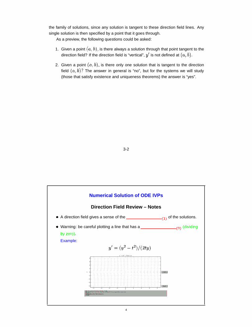
Numerical Solution of ODE IVPs
Direction Field Review – Notes
� A direction field gives a sense of the ����� of the solutions.
� Warning: be careful plotting a line that has a � � � (dividing
by zero).
Example:� ��� � � � � � � $���� ����
−4 −3 −2 −1 0 1 2 3 4
−4
−3
−2
−1
0
1
2
3
4
t
y
y ’ = (y2 − t2)/(2 t y)
4

Numerical Solution of ODE IVPs
Notes for Direction Field Review Notes slide:
Answers:
(1) flow
(2) vertical slope
The ODE example has a singularity at ����� and at ��� . Try making a direction
field for ����� ���� and ���� ���� . Try this in any demo package you like. You’ll
find that you can create the direction field, but if you try to draw the solution near to the
singularity, the generation of the solution path may get stuck.
4-1
Numerical Solution of ODE IVPs
Existence and Uniqueness: A Reminder
Questions we must ask:
� Is there a solution?
� Is there only one solution?
Why are these questions important?
1. If there is ����� , your computer program may
� � � .2. If there is � ��� , the program will
� ��� . It may not be the one you want.
From your ODEs course, you learned theorems that gave checklists ensuring the
existence and uniqueness of ODE IVP solutions.
A TIP: Use these theorems.
5
Numerical Solution of ODE IVPs
Notes for Existence and Uniqueness A Reminder slide:
Answers:
(1) no solution
(2) still produce output
(3) more than one solution
(4) choose a solution for you
The students should already have been exposed to the theorems regarding exis-
tence and uniqueness of solutions. If you feel it is appropriate, you may provide hand-
outs that summarize these theorems. You may wish to point out to the students that the
more serious computing we do, the more we must rely on fundamental mathematical
theory to inform us about the validity of our computed solutions.
Possible Example: You may wish find an example for which the computational out-
put is incorrect, and the theory shows that you are likely to get into trouble (e.g., if there
are multiple solutions). For example, � � ��� � ��� � (or use any power less than � ) and
initial data � � � ����� . This has � �"����� as a solution, but also � �"� � � is a solution.
What would a numerical solver do with this problem?
5-1
Numerical Solution of ODE IVPs
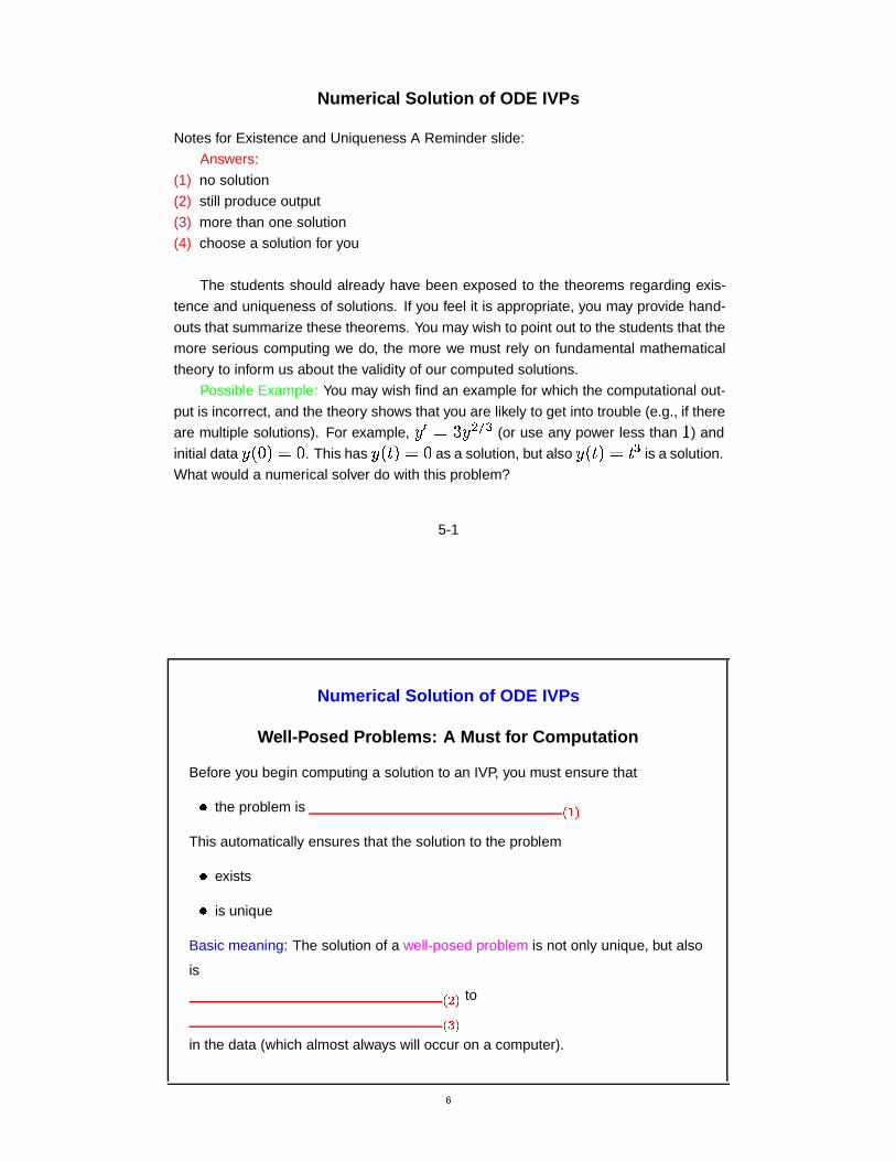
Well-Posed Problems: A Must for Computation
Before you begin computing a solution to an IVP, you must ensure that
� the problem is �����This automatically ensures that the solution to the problem
� exists
� is unique
Basic meaning: The solution of a well-posed problem is not only unique, but also
is
��� � to� ���
in the data (which almost always will occur on a computer).
6

Numerical Solution of ODE IVPs
Notes for Well-Posed Problems A Must for Computation slide:
Answers:
(1) well-posed
(2) not too sensitive
(3) small perturbations
Note: To make computation of an accurate solution feasible, not only must an ODE
IVP have a solution that exists and is unique, but the problem must also be well-posed.
A mathematical problem is well-posed if in addition to existence and uniqueness, the
solution also depends continuously on the problem data. This will be formally defined
on the next slide.
Well-posedness is very important because if the solution to the perturbed ODE is
very different from the unperturbed solution, it is very difficult to get a good computa-
tional answer. So, for the students, well-posedness is a necessity.
In reality, well-posedness of a problem is considered highly desirable, but is not
always achievable. For example, the problem of determining an illness based on symp-
toms is not well posed, since the same set of symptoms (e.g., stomach ache) can be
6-1
the result of more than one cause (food poisoning, viral infection, bacterial infection,
etc.). Heath [Hea02, p. 3] points out that inferring the internal structure of a physical
system solely from external observations , as in tomography or seismology, often leads
to mathematical problems that are inherently ill-posed in that distinctly different internal
configurations may have indistinguishable external appearances.
6-2
Numerical Solution of ODE IVPs
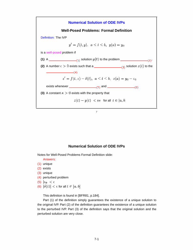
Well-Posed Problems: Formal Definition
Definition: The IVP
� ��������� � � ���� � � � �!�!� ��� ���
is a well-posed problem if
(1) A ���� solution � �"� to the problem ��� � .(2) A number ��� � exists such that a � ��� solution � �"� to the
� ���� � ������ � � ���� �"� ���� � � � � ��� � � ���� � �
exists whenever ��� � and �� ��(3) A constant ��� � exists with the property that
� � �"�����!�"� ��� ��� for all ���� �������
7
Numerical Solution of ODE IVPs
Notes for Well-Posed Problems Formal Definition slide:
Answers:
(1) unique
(2) exists
(3) unique
(4) perturbed problem
(5)� � � ��� �
(6)� � �"� ��� � for all ���� �������
This definition is found in [BFR81, p.184].
Part (1) of the definition simply guarantees the existence of a unique solution to
the original IVP. Part (2) of the definition guarantees the existence of a unique solution
to the perturbed IVP. Part (3) of the definition says that the original solution and the
perturbed solution are very close.
7-1

Numerical Solution of ODE IVPs
Well-Posed Problems: An Easy Test?
Question: How can we tell whether criteria ������� ���� for
well-posedness are satisfied for a particular problem?
Answer: Good news! There is an easy test (i.e., a
theorem) that tells us immediately whether an IVP is
well-posed.
8
Numerical Solution of ODE IVPs
Well-Posed Problems: An Easy Test!
Theorem: Suppose ������� � � � � � ������� and � � �� � # ��� . The IVP
# �# ������� �������� � � ��� � � �!��� ��� ���
is well-posed provided
1. � is ����� on 2. � satisfies a ��� � in the variable
����� on the set � ���
9

Numerical Solution of ODE IVPs
Notes for Well-Posed Prolems An Easy Test slide:
Answers:
(1) continuous
(2) Lipschitz Condition
(3) �(4)
This test for well-posedness is found in [BFR81, p.184].
� These conditions are sufficient conditions.
� With this theorem, we only need to test the right-hand-side ����� ��� of the ODE,
we do not need to find any a priori solutions.
� The next slide explains what a Lipschitz condition is. The students may not have
seen this before.
Comments from [Gea71, p.7]: In many problems we cannot get a Lipschitz condi-
tion for all � , but only in a region of the � -space. [For example, if ����� ��� � � � , � �!$ � �
9-1
exists and is bounded in any finite region.] The proof of this Lipschitz theorem is valid as
long as both � and � remain in the region, so it may be necessary to limit the maximum
perturbation � . For example, perturbations to � � � � $ � � � �!� � � � � , are bounded as
long as the perturbation does not reduce � below � . Consequently, it is well posed with
respect to any positive initial value � � , but when � � is close to � , � is small and � is
large.
9-2
Numerical Solution of ODE IVPs
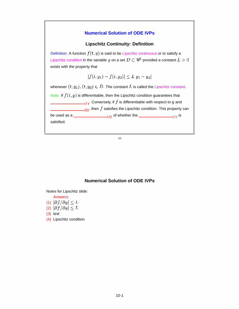
Lipschitz Continuity: Definition
Definition: A function ����� � � is said to be Lipschitz continuous or to satisfy a
Lipschitz condition in the variable � on a set ���� � provided a constant � � �exists with the property that
� ����� � � ��� ���� � � � � � � � � � � � � � �
whenever ��� � � � � ��� � � � � . The constant � is called the Lipschitz constant.
Note: If ����� � � is differentiable, then the Lipschitz condition guarantees that
����� . Conversely, if � is differentiable with respect to � and
��� � , then � satisfies the Lipschitz condition. This property can
be used as a � ��� of whether the � ��� is
satisfied.
10
Numerical Solution of ODE IVPs
Notes for Lipschitz slide:
Answers:
(1)�
� �!$ � � � � �(2)
�� �!$ � � � � �
(3) test
(4) Lipschitz condition
10-1

Numerical Solution of ODE IVPs
Lipschitz Condition Test: Example
Example: Determine whether the IVP � � ������� ��� ���!� � � � ��� on is well
posed, given����� ��� � �
and
������ � � � � ��� � � � � �!� ��� � � � � � �If so, find the Lipschitz constant.
Answer: For each ��� � � � � �� � � � � in , we have
� ����� � � ��� ����� � � � � � � �� � �� � � � � � � � � � � � � � � � � � � � �
So, ����� ��� is ����� in � � � on
� ��� , with Lipschitz constant � � � ��� .
11
Numerical Solution of ODE IVPs
Notes for Lipschitz Example slide:
Answers:
(1) Lipschitz continuous
(2) �(3) (4) �
The example was borrowed from [BFR81, p. 182].
11-1

Numerical Solution of ODE IVPs
Well-Posed versus Stable Solutions (1)
Question: How much can a perturbed solution��� �� � with perturbed
�� � ��� ��� � and
perturbed initial conditions��� � � � � ��� � ���� from the original
solution�� �"� with original
�� �� � �� � and original initial conditions�� �� � � � �� �
when ��� � continuity with constant � on a bounded domain is assumed?
Answer:
��� ��� �"� � �� �� � � � ����� ������ �� ��� ��� � � �� � � � � � � ������ �� � ��
� � �� � � �� � �
where��� �� � � �� ��� ������� ����� �� ����� � � �� � ��� �� ��� �� �� � �� � ��� �
12
Numerical Solution of ODE IVPs
Notes for Well-Posed versus Stable (1) slide:
Answers:
(1) differ
(2) Lipschitz
Note: The bound on the difference between the original solution and the perturbed
solution is derived in [Hea02, p.388]. It is not necessary to go into detail here. However,
it may be useful to point out to the students that the first additive portion of the bound
is due to perturbations in the initial data, while the second additive portion is due to
perturbations in the function��.
Note: Even a well-posed problem may have perturbed solutions that diverge ex-
ponentially over time. Therefore, we also talk about solutions of ODEs that are stable
and asymptotically stable, for which perturbed solutions do not diverge by more than a
constant amount over time. Make sure to point out to the students that the word “stable”
is commonly used both to refer to the sensitivity of solutions of an ODE and to refer
to the sensitivity of a numerical algorithm. So we can have a “stable solution”, and we
can have a “stable algorithm”. This can initially be confusing to students. However, they
12-1
are likely to see these two uses for the word “stable” in textbooks and other literature.
Stability of numerical algorithms will be discussed in later slides.
Note: This slide and the next slide on the stability of an ODE solution may beskipped if you wish.
12-2
Numerical Solution of ODE IVPs
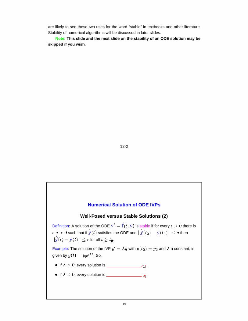
Well-Posed versus Stable Solutions (2)
Definition: A solution of the ODE�� � � �� �� � �� � is stable if for every ��� � there is
a � � � such that if��� �"� satisfies the ODE and
� � ��� � � ��� �� � � � ��� � � then� � ��� �"��� �� �"� ��� � � for all �� � �
Example: The solution of the IVP � � ����� with � � � � � ��� and � a constant, is
given by �!�"��� � � ��� � � So,
� If � � � , every solution is ���� .� If �
� � , every solution is � � � .
13
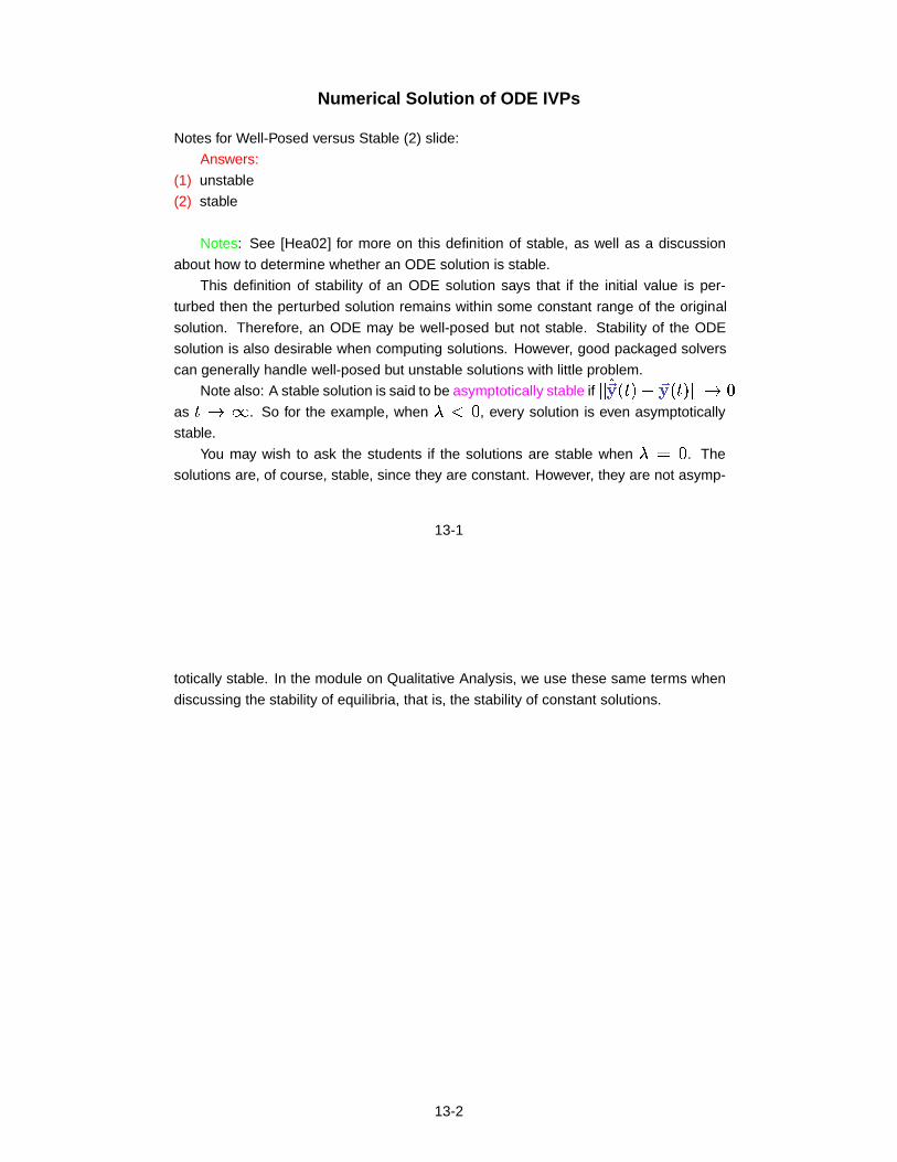
Numerical Solution of ODE IVPs
Notes for Well-Posed versus Stable (2) slide:
Answers:
(1) unstable
(2) stable
Notes: See [Hea02] for more on this definition of stable, as well as a discussion
about how to determine whether an ODE solution is stable.
This definition of stability of an ODE solution says that if the initial value is per-
turbed then the perturbed solution remains within some constant range of the original
solution. Therefore, an ODE may be well-posed but not stable. Stability of the ODE
solution is also desirable when computing solutions. However, good packaged solvers
can generally handle well-posed but unstable solutions with little problem.
Note also: A stable solution is said to be asymptotically stable if��� ��� �"��� �� �� � � ��� �
as � �
. So for the example, when �� � , every solution is even asymptotically
stable.
You may wish to ask the students if the solutions are stable when � � � . The
solutions are, of course, stable, since they are constant. However, they are not asymp-
13-1
totically stable. In the module on Qualitative Analysis, we use these same terms when
discussing the stability of equilibria, that is, the stability of constant solutions.
13-2
Numerical Solution of ODE IVPs
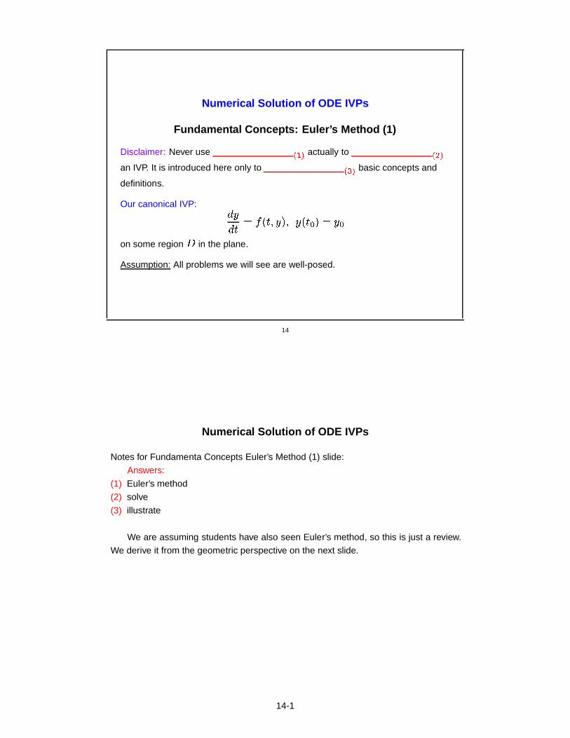
Fundamental Concepts: Euler’s Method (1)
Disclaimer: Never use ����� actually to ��� �an IVP. It is introduced here only to � ��� basic concepts and
definitions.
Our canonical IVP:# �# ������� ��� � �!� � � � ���
on some region in the plane.
Assumption: All problems we will see are well-posed.
14
Numerical Solution of ODE IVPs
Notes for Fundamenta Concepts Euler’s Method (1) slide:
Answers:
(1) Euler’s method
(2) solve
(3) illustrate
We are assuming students have also seen Euler’s method, so this is just a review.
We derive it from the geometric perspective on the next slide.
14-1

Numerical Solution of ODE IVPs
Fundamental Concepts: Euler’s Method (2)
(t1,y1)
Direction Field Arrow:Take one step in this direction
Start Point(t0,y0) }
Step size h
}t1 = t0 + hy1 = y0 + dy = y0 + h*f(t0,y0)
Slope = f(t0,y0)Height = f(t0,y0)*h
In general: Starting at � � � ��� � , we get to ����� � � ����� � � by using
���� � � �� ���
����� � � ��� ��� ����� � ����
Note: ���� � represents the numerical approximation to �!���� � � .Euler’s method is: ����� and ��� � .
15
Numerical Solution of ODE IVPs
Notes for Fundamental Concepts Euler’s Method (2) slide:
Answers:
(1) single-step
(2) explicit
Note:
� A “multi-step” method includes more “history”. That is, one would see functions
of �� as well as �� � , �� � , etc. on the right-hand-side of the ODE.
� An “implicit” method would have a function of ���� � � ����� � � on the right-hand-
side of the ODE.
Suggestion: You may want to insert a demo here (in MATLAB, for example) of an
implementation of Euler’s method. One good example to try:
��� � � � � � � � �� � � � � �� � � � � �
15-1

Actual solution is � �"� � ��� � . Try step size � ��� � � , so �� ��� � ��� . This example
is borrowed from [BFR81, p.188]. Euler’s method works fine for this simple example.
MATLAB demo code: See NumDemo1 scripts.
15-2
Numerical Solution of ODE IVPs
Truncation Error
Truncation Error (TE) arises from the �����of the true solution.
Usually, a ��� � or � ��� summation
approximates an � ��� .Example: Taylor expand �!�� ��� � � to get Euler’s Method (a type of “Taylor
Method”):
�!������ � � � � ��� ����� � � ��� �� ��� �
Euler’s Method: Truncated Series
� � ��� � � ���� � ��� ��� � �
� ��� �Local Truncation Error (LTE)
16

Numerical Solution of ODE IVPs
Notes for Truncation Error slide:
Answers:
(1) mathematical approximation
(2) finite
(3) truncated
(4) infinite series
Using the Taylor expansion of � � ��� � � is an alternate way to derive Euler’s method.
Truncation Error (TE) is the error that arises because of the mathematical approximation
to the actual solution. TE usually refers to error arising from using a truncated or finite
summation to approximate the sum of an infinite series. In the case of Euler’s method,
the infinite series is a Taylor expansion. Euler’s method is considered a type of “Taylor
Method”. Euler’s method truncates the Taylor series after two terms. Higher order
Taylor methods truncate the series after more terms have been included. Note that we
are implicitly assuming that � �"� is analytic, that is, that it has a Taylor series expansion.
16-1
Numerical Solution of ODE IVPs
Order of a Method
Generally, Local Truncation Error (LTE) can be approximated by � ��� in the sense
that ��� ���� � LTE ������ � � �
In general: The number � � � is the order of the numerical method.
Example: Let � � be the numerical approximation to �!� � � . Then LTE in Euler’s
method is:� � � ����� � �
� ����� � � � � ������� � � � �
Here, � � ����� , so Euler’s method is order ��� � .Terminology:
An order � ��� method implies:
The � ��� error behaves like ��� � .
17

Numerical Solution of ODE IVPs
Notes for Order of a Method slide:
Answers:
(1) �
(2) �(3) �(4) accumulated
(5) � �
The “order of a method” reveals the global or accumulated error in a method. The
Local Truncation Error LTE depends on the step-size � and the method begin used. For
Euler’s method, for example, LTE shrinks like � ��� � � as � shrinks, and Euler’s method
is “order 1”. The larger � is (which changes with the method) the better. The global or
accumulated error behaves like � in the case of Euler. So, if we were to halve � , our
global error would be halved (not counting rounding). For an order � method, halving �
would cut our global error to � $ � its previous size.
17-1
Numerical Solution of ODE IVPs
Summary: Types of Numerical Error
� Rounding error: From finite precision floating point arithmetic.
(Example:���� � � � � � � )
� Truncation error: From the method used. Two classes:
� Local (LTE): Error made in ����� of the numerical
method.
� Global (GTE): Accumulated error. Error made after
��� � of the numerical method.
� A numerical method is “order � ” if LTE = � ������ � � .
18
Numerical Solution of ODE IVPs
Notes for Types of Numerical Error slide:
Answers:
(1) one step
(2) several steps
“Truncation error” is also sometimes referred to as “Discretization error”. TE arises
from the method used, and would remain even if the floating point arithmetic were per-
fect.
LTE: � � � � � � � where �!� � � is the true solution of the ODE passing through the
previous point � � � ��� � .GTE: � � � � ����� � ��� where � ��� � is the true solution of the ODE passing
through the initial point � � � ��� � .Note: An exercise to try: Confirming the order of a method. See e.g. [Dan85, p.
21]. Also try with second or fourth order Runge-Kutta.
18-1
Numerical Solution of ODE IVPs
Stability of a Numerical Method: Introductory Example
Idea: If ����� do not cause the
��� � solution to diverge from the � ���solution, the numerical method is stable.
Example: Given the test IVP
� ��� � � � � � � ��� ���
apply Euler’s method with step size � ��� :����� � � ��� � � � ��� � � � ��� � �����
which implies that����� � � � � ��� � �
� ��� �Amplification Factor
��� � ���
19
Numerical Solution of ODE IVPs
Notes for Stability:Introductory Example slide:
Answers:
(1) small perturbations
(2) numerical
(3) true
(4) �
Essentially: If small perturbations do not cause the resulting numerical solution to
diverge away without bound, the method is considered stable.
The example problem given in this slide is well-posed. This is the canonical IVP
on which stability of numerical methods is often tested. If a method is stable on this
problem, it is likely to be stable on more complicated problems. The exact solution to
the IVP is �!�"� � � � � � � .
19-1
Numerical Solution of ODE IVPs
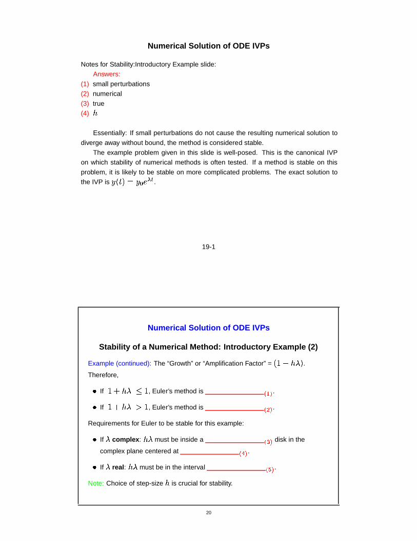
Stability of a Numerical Method: Introductory Example (2)
Example (continued): The “Growth” or “Amplification Factor” = � � ��� � � .Therefore,
� If�� ��� � � � � , Euler’s method is ����� .
� If�� ��� � � � � , Euler’s method is ��� � .
Requirements for Euler to be stable for this example:
� If � complex: � � must be inside a ����� disk in the
complex plane centered at � ��� .� If � real: � � must be in the interval ��� � .
Note: Choice of step-size � is crucial for stability.
20
Numerical Solution of ODE IVPs
Notes for Stability(2) slide:
Answers:
(1) stable
(2) unstable
(3) radius �(4) � �(5) ��� � � � �
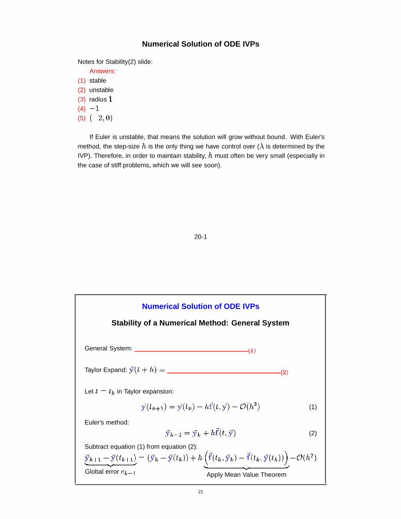
If Euler is unstable, that means the solution will grow without bound. With Euler’s
method, the step-size � is the only thing we have control over ( � is determined by the
IVP). Therefore, in order to maintain stability, � must often be very small (especially in
the case of stiff problems, which we will see soon).
20-1
Numerical Solution of ODE IVPs
Stability of a Numerical Method: General System
General System: �����
Taylor Expand:�� � � ��� � � � �
Let � �� in Taylor expansion:
�� ��� � � � � �� ��� ����� �� ��� �� � ��� ��� � � (1)
Euler’s method:�� � � � � �� � � � �� ��� �� � (2)
Subtract equation (1) from equation (2):�� � � � � �� ��� � � �� ��� �Global error ��� � �
� � �� � � �� ��� � � � �� �� ������ �� � ��� �� ��� � �� ��� �"���� ��� �Apply Mean Value Theorem
� � ��� � �
21

Numerical Solution of ODE IVPs
Notes for Stability General System slide:
Answers:
(1)�� � � �� ��� �� � .
(2)�� �"� � � �� � �"�
� ��� ��� ����� �� �
� � ��� � �
So what can we say about a more general system of ODEs? At this point, we
introduce the notion of stability in the context of a system, because the only difference
here between a system and a single equation is the notation. All concepts carry over.
21-1
Numerical Solution of ODE IVPs
Stability of a Numerical Method: General System (2)
Applying the Mean Value Theorem:�� ����� �� � ��� �� ��� � �� ��� � � � � ����� � � �� � ��� � � � � �� ��� � � � �� � � �� ��� � �
where
� � � � ����� matrix of��
w.r.t.�� and � � � � � � ���
��� � is expressed in general as:
�� � � � � � � ��� � � �� ��� �
Amplification Factor
�� ��� LTE � � �
Requirement for � ��� :� � � ��� � � � �
where � represents the � ��� of a matrix.
22
Numerical Solution of ODE IVPs
Notes for Stability General System (2) slide:
Answers:
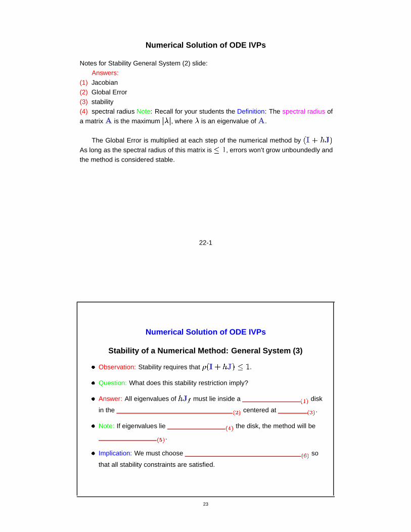
(1) Jacobian
(2) Global Error
(3) stability
(4) spectral radius Note: Recall for your students the Definition: The spectral radius of
a matrix � is the maximum� � � , where � is an eigenvalue of � .
The Global Error is multiplied at each step of the numerical method by � � � � � �As long as the spectral radius of this matrix is � � , errors won’t grow unboundedly and
the method is considered stable.
22-1
Numerical Solution of ODE IVPs
Stability of a Numerical Method: General System (3)
� Observation: Stability requires that � � � � � � � � � .� Question: What does this stability restriction imply?
� Answer: All eigenvalues of � � � must lie inside a ���� disk
in the ��� � centered at � ��� .� Note: If eigenvalues lie � ��� the disk, the method will be
� � � .� Implication: We must choose � �� so
that all stability constraints are satisfied.
23

Numerical Solution of ODE IVPs
Notes for Stability General System (3) slide:
Answers:
(1) radius �(2) complex plane
(3) � �(4) outside
(5) unstable
(6) step size �
23-1
Numerical Solution of ODE IVPs
Stability of a Numerical Method:
Euler Method Region of Stability
All eigenvalues of � � � must lie inside the disk.
−1
Re
Im
Region of Stabilityfor Forward EulerMethod
24

Numerical Solution of ODE IVPs
Stability of a Numerical Method: Euler Example
Example: Consider
� ��� � � � � � � � � � �!� � � � � �� � ��� � � � �
Question: When will Euler’s Method be stable?
Answer: Notice that EM implies
� � � � � � � ���!� � � � ��� � � � � � � � � � � � � � � � � �� ��� �Amplification Factor
� �
Therefore,
� For ����� , the method is unstable for any ��� � .� For � ��� , the method will be stable if � ��� .
25
Numerical Solution of ODE IVPs
Notes for Stability - Euler Example slide:
Answers:
(1) � �(2) �
(3) � �(4) � � ��
� ��� � �
Example borrowed from [KMN89, p.289]. Note that in this example, � is required to
get smaller and smaller as grows. Therefore, for a fixed � , we can expect the method
to become unstable after a certain point in time.
25-1
Numerical Solution of ODE IVPs
Stability of a Numerical Method: Euler Example Illustration
0 1 2 3 4 5 6−0.5
0
0.5
1
Time t
Solut
ion y(
t)
EM h = 0.10001, ODE dy/dt = −10(t−1)y, y0 = 0.00673795
Euler solverTrue Solution
26
Numerical Solution of ODE IVPs
Notes for Euler Example Illustration slide:
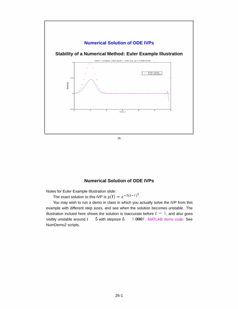
The exact solution to this IVP is � �"� � � �� ��� ����� �You may wish to run a demo in class in which you actually solve the IVP from this
example with different step sizes, and see when the solution becomes unstable. The
illustration inclued here shows the solution is inaccurate before � � , and also goes
visibly unstable around ��� with stepsize � � � � � � � � . MATLAB demo code: See
NumDemo2 scripts.
26-1
Numerical Solution of ODE IVPs
Implicit Methods
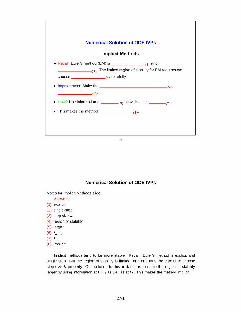
� Recall: Euler’s method (EM) is ����� and
� � � . The limited region of stability for EM requires we
choose � ��� carefully.
� Improvement: Make the � ���� � � .
� How? Use information at � �� as wells as at ��� � .� This makes the method ����� .
27
Numerical Solution of ODE IVPs
Notes for Implicit Methods slide:
Answers:
(1) explicit
(2) single-step
(3) step size �
(4) region of stability
(5) larger
(6) �� � �(7) ��(8) implicit
Implicit methods tend to be more stable. Recall: Euler’s method is explicit and
single step. But the region of stability is limited, and one must be careful to choose
step-size � properly. One solution to this limitation is to make the region of stability
larger by using information at � � � as well as at �� . This makes the method implicit.
27-1

Numerical Solution of ODE IVPs
Implicit Methods: Backward Euler
� Example of an Implicit Method: Backward Euler Method (BE)
�� � � � � �� � ��� �� ��� � � � �� � � �� ��� �Implicit
�
� Question: How can we solve for�� � � � ?
� Answer:
� Use ���� . This often requires calculating the
��� � of the function�� ��� �� � .
� Use ����� methods.
� Note: Both approaches require an initial guess, usually derived by taking one
step of an explicit method.
28
Numerical Solution of ODE IVPs
Notes for Implicit Methods BE slide:
Answers:
(1) root-finding
(2) derivative or Jacobian
(3) predictor-corrector
The example we provide is the Backward Euler (BE) method. This introduces the
additional complication of figuring out how to solve a possibly nonlinear equation for
its root. The question about solving for�� � � � is important, especially if the right hand
side�� ��� �� � of the ODE is nonlinear in
�� . One can use a built in root finder, or write
ones own code. Using a built-in root finder is a good way to go, if the root finder is
given a sufficiently close initial guess. However, how many iterations a root-finder will
need per time step may become large in some cases. It is also common to implement
Predictor-Corrector methods in this case. These are very easy to write and implement,
and may take fewer steps per iteration, but one must be very careful of issues involving
convergence of the method.
28-1
Numerical Solution of ODE IVPs
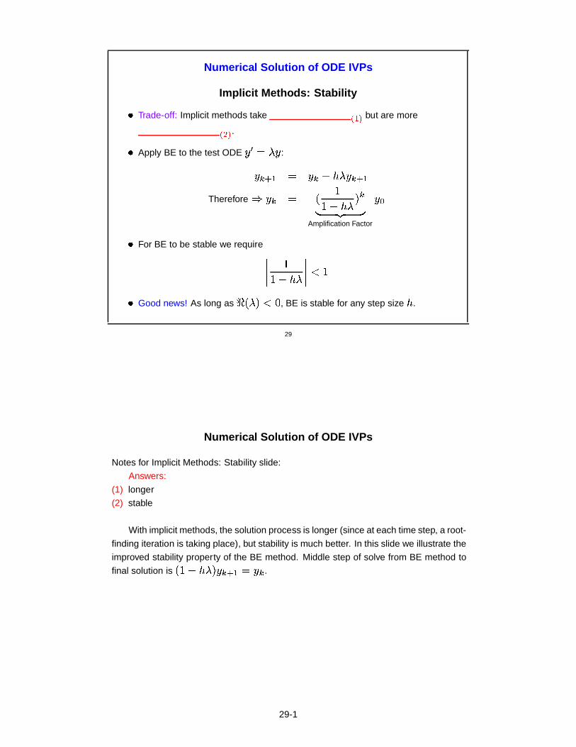
Implicit Methods: Stability
� Trade-off: Implicit methods take ���� but are more
� � � .� Apply BE to the test ODE � � � ��� :
� � � � � � � � � ��� � � �Therefore � � � � � �
� � � �� �
� ��� �Amplification Factor
���
� For BE to be stable we require����
�� � � �
������
� Good news! As long as � � � � � � , BE is stable for any step size � .
29
Numerical Solution of ODE IVPs
Notes for Implicit Methods: Stability slide:
Answers:
(1) longer
(2) stable
With implicit methods, the solution process is longer (since at each time step, a root-
finding iteration is taking place), but stability is much better. In this slide we illustrate the
improved stability property of the BE method. Middle step of solve from BE method to
final solution is � � � � � � � � � � � � � .
29-1
Numerical Solution of ODE IVPs
Stability of a Numerical Method: BE Stability Region Illustration
All eigenvalues of � � � must lie in the left half plane.
������������������������
������������������������
Region of Stabilityfor Backward Euler Method
Re
Im
Entire Left Half Plane
30
Numerical Solution of ODE IVPs
Implicit Methods: Stability Notes
Notes:
� BE is ����� accurate (just like ��� � )� For a � ��� , the stability requirement becomes
� � � � � � � � � � � � �� The stability region for BE is the entire � ��� of the complex
plane (as compared to the radius 1 disk of EM).
� Since ��� � step size � keeps us within the stability region, the BE
method is called � �� .� There exist higher order implicit methods, like the Trapezoid Method (order =
� � � ).� Not all implicit methods are � ��� .
31

Numerical Solution of ODE IVPs
Notes for Implicit Methods: Stability Notes slide:
Answers:
(1) 1st order
(2) EM
(3) system
(4) left half
(5) any
(6) unconditionally stable
(7) �
(8) unconditionally stable
An example of a higher order implicit method that is also unconditionally stable is
the Trapezoid method:
� � � � � � ��� � � �������� � � � � ����� � � � � � � � � � $ �The Trapezoid Method is second order accurate and unconditionally stable for all eigen-
values in the LHS of the complex plane. The Trapezoid method is also known as 2nd
31-1
order Adams-Moulton. Not all implicit methods are unconditionally stable, but they do
tend to have larger regions of stability than do explicit methods.
31-2

Numerical Solution of ODE IVPs
Stiffness in ODEs
Question: What is “stiffness”?
Answer:
� Physically: A process whose components have ����� time
scales. Also, a process whose time scale is � � � compared
to the time interval over which it is being observed.
� Mathematically: A well-posed ODE�� � � �� ��� �� � is “stiff” if its Jacobian � �
has � ��� that differ greatly in magnitude.
� Practically: An ODE is stiff if an explicit method (like EM) is
� ��� because stability requirements force the step size � to
be extremely small.
32
Numerical Solution of ODE IVPs
Notes for Stiffness in ODEs slide:
Answers:
(1) highly disparate
(2) short
(3) eigenvalues
(4) inefficient
Note: Some of these observations were borrowed from [Hea02, p. 401]. The
requirement that step-size � be extremely small for stability of stiff problems is undesir-
able because it is usually smaller than one would need � to be to achieve reasonable
accuracy.
32-1

Numerical Solution of ODE IVPs
Stiffness in ODEs: Example 1
Example 1: For test ODE � � � ��� with � � � ��� � , the problem is
����� if ��� � .Recall: For stability in EM, we require
�� � � � � � � . If � is real and �
� � � � ,this forces ����� .For a system: A system of ODEs with ���� ������� is � ��� when
��� � where ��� are the
� �� of Jacobian � ��� �� �� �"� .
33
Numerical Solution of ODE IVPs
Notes for Stiff ODEs Example 1 slide:
Answers:
(1) stiff
(2) �!� � � � � � � � � � � �(3) � to be very small
(4) stiff
(5) �!� � � � � ��� � � � � ��� � � � � � �(6) eigenvalues
33-1

Numerical Solution of ODE IVPs
Stiffness in ODEs: Example 2
Example 2: Consider
� � � � � � � ��� ��� "� ���������� �!� � ��� � � ���� � � � �Let � � � � � � . Then the Jacobian is ����� . So eigenvalue � �
��� � . Therefore,
� � � � � � � � ��� � � � � � � � � � � � � � �This is � ��� on ��� � � � � .Note: on another interval, ���� � � � � � � � � we have
� � � � � � � � � � � � � � � � � � � � � � � � � � � ��� � �
so this ODE is � ��� on this interval.
34
Numerical Solution of ODE IVPs
Notes for Stiff ODEs Example 2 slide:
Answers:
(1)� ��� � � �
(2) �(3) stiff
(4) not stiff
Example 2 borrowed from [KMN89, p. 285].
34-1

Numerical Solution of ODE IVPs
Stiffness: EM vs BE
Consider��� � � � � � � � � � � � � � � � � � � � � �
Let � ��� � � . Computed output with perturbed initial data:
Time � � � � � � � � � � � � � � � � � � � �
Exact Soln� ����� � � � � � ����� � ���� � ����
EM � �� � � � � � � �� � � �� ��� � � � �
EM � � � � � � � � � � � � � � �� � ��� � � �
BE � � � � � � � � � � � � � � � � � � �
BE � � � � � � � � � � � � � � � � � � �
35
Numerical Solution of ODE IVPs
Notes for EM vs BE slide:
This example was borrowed from [Hea02, p. 402]. The general solution to the ODE
is � �"��� � � � � � � � � . In general, �!� � ��� � � . But with � � � � � � , this implies ��� . The problem is stiff.
We have MATLAB code that solves this problem, both with EM and BE. The data in
the table are taken from the MATLAB code, and are confirmed in Heath [Hea02, p.402].
MATLAB demo code: See NumDemo3 scripts.
Note that we have not addressed stiff problems with rapidly oscillating solutions.
The approach there would be different. See suggestions in Stoer and Bulirsch.
35-1

Numerical Solution of ODE IVPs
Stiffness: Comments on EM vs BE
Note:
� EM ���� with only � � � perturbations.
� BE is � ��� even with � ��� perturbations.
36
Numerical Solution of ODE IVPs
Notes for Stiffness:Comments slide:
Answers:
(1) breaks down
(2) small
(3) robust
(4) large
36-1

Numerical Solution of ODE IVPs
Stiffness: Summary
� A particular ODE may be ����� or ��� � .� A numerical ODE solving method can be � ��� or
� ��� for a particular problem.
� The stability of the numerical method often depends on
� � � .� �� �� methods should (almost) always be used to solve stiff
ODEs.
37
Numerical Solution of ODE IVPs
Notes for Stiffness:Summary slide:
Answers:
(1) stiff
(2) nonstiff
(3) stable
(4) unstable
(5) the step-size �
(6) Implicit
We say that implicit methods should almost always be used to solve stiff ODEs,
because the degree of stiffness can vary. It is possible to encounter a somewhat stiff
problem that can be solved by using automatic step size adjustment with an explicit
method. However, it is usually wisest to stick with the implicit methods when there is
stiffness in the ODE.
37-1

Numerical Solution of ODE IVPs
Other IVP Solvers
Other classes of numerical IVP solvers include (but are not limited to):
� Higher Order Taylor methods (seldom used)� Can give ���� accuracy.
� They require the computation of the ��� � of ����� ��� .� Runge-Kutta methods (very popular)
� Can give ����� accuracy.
� Do not need � ��� of ���� � � � .� Can be ��� � or � �� .� These are ��� � -step methods.� Methods include: Midpoint, Modified Euler, Heun, 4th Order
Runge-Kutta (RK4)
38
Numerical Solution of ODE IVPs
Notes for Other IVP Solvers slide:
Answers:
(1) high
(2) derivatives
(3) high
(4) derivatives
(5) explicit
(6) implicit
(7) single
Notes: High order Taylor methods have not been so popular because they involve
calculating the derivative of your function. However, in the future, newer automatic
differentiation methods may allow for increased use of High order Taylor methods.
38-1

Numerical Solution of ODE IVPs
Other IVP Solvers (cont)
� Multi-step methods
� Can give ���� accuracy.
� Can be ��� � or � ��� .� Starting values must be calculated with a � ���method (e.g., RK4)
� Methods include: Adams-Bashforth, Adams-Moulton, Milne, Simpson
� Extrapolation methods
� These take solutions generated by lower order methods, and increase
��� � by � �� .� Variations of these methods presented in [SB93], [Ste73], and [Gra65].
Also see the discussion and reference list in [Asa95, p.642].
39
Numerical Solution of ODE IVPs
Notes for Other IVP Solvers slide:
Answers:
(1) high
(2) explicit
(3) implicit
(4) single-step
(5) accuracy
(6) extrapolation
39-1

Numerical Solution of ODE IVPs
Systems and Higher Order IVPs
� All methods and theories presented can be ����� to apply to
systems.
� Many higher order IVPs can be ��� � to 1st order systems
of IVPs. Then all methods and theories apply here, too.
Example: Suppose we have the second order equation describing a linear spring,
��� ��� � � � � �!� � ��� � � � ��� � � � ��� �Convert this to a ��� � first order system of equations:
��� � �
� � � � ���
40
Numerical Solution of ODE IVPs
Notes on Systems slide
Answers:
(1) directly generalized
(2) converted
(3) � � �Every ODE solving concept we have discussed to this point can be extended to
solving systems of 1st order ODE IVPs. This implies that higher order IVPs that can
be converted to a first order system can also be solved with the same techniques and
theories. Students should already have seen how to do this kind of conversion in their
introductory ODE class. If there is a need to refresh their memory, it may be appropriate
to show a couple of simple examples. In sum: Methods to solve 1st order systems of
ODEs are simply generalizations of the methods for a single 1st order equation.
40-1

Numerical Solution of ODE IVPs
Solving IVPs with Packaged Software
To solve a system of ODE IVPs�� � � �� �� � �� � with �!� � � � ��� with a packaged
routine typically requires ����� to supply the following:
� The name of the routine that computes�� �� � �� � .
� � � � and � ��� values for times .� Initial value � � .����� and for some solvers, sometimes ������ The number of equations in the system.
� � ��� and/or ��� � error tolerances.����� and sometimes for a stiff ODE ������ The routine that computes the Jacobian � � of function
��.
41
Numerical Solution of ODE IVPs
Notes on Packaged Software slide
Answers:
(1) the user
(2) Initial
(3) final
(4) Absolute
(5) relative
Note: The output for many of these solvers usually includes the solution�� at the final
time , but can often include a whole string of solutions�� at various times . Some
solvers may also provide warning messages, or measures of the quality of the solution
generated.
At this point it might be a good idea to provide some actual codes for the students to
look at. For example, in MATLAB, one could provide a file in which the ODE is defined,
as well as a file that calls a standard MATLAB solver, like ODE45. This is a good point to
assign some exercises, as well. One type of exercise might involve having the students
solve various IVPs and IVP systems using some built-in solvers, and then comparing
accuracy and speed.
41-1

References
[Asa95] N. S. Asaithambi. Numerical Analysis: Theory and Practice. Saunders COl-
lege Publishing, 1995.
[BFR81] Richard L. Burden, J. Douglas Faires, and Albert C. Reynolds. Numerical
Analysis. Prindle, Weber & Schmidt, second edition, 1981.
[Dan85] J. M. A. Danby. Computing Applications to Differential Equations. Reston
Publishing Company, 1985.
[Gea71] C. William Gear. Numerical Initial Value Problems in Ordinary Differential
Equations. Prentice-Hall Series. Prentice-Hall, 1971.
[Gra65] W. Gragg. On extrapolation algorithms for ordinary initial value problems.
SIAM Journal on Numerical Analysis, 2:384–403, 1965.
[Hea02] Michael T. Heath. Scientific Computing: An Introductory Survey. McGraw
Hill, second edition, 2002.
41-2
[KMN89] David Kahaner, Cleve Moler, and Stephen Nash. Numerical Methods and
Software. Prentice Hall Series in Computational Mathematics. Prentice-Hall,
1989.
[SB93] J. Stoer and R. Bulirsch. Introduction to Numerical Analysis. Springer, second
edition, 1993.
[Ste73] H.J. Stetter. Analysis of discretization methods for ordinary differential equa-
tions. In Tracts in Natural Philosophy. Springer, 1973.
41-3
Top Related