


Languages
Pages
Legal


Numerical Prediction of Pitch Damping Stability Derivatives
for Finned Projectiles
by Vishal A. Bhagwandin and Jubaraj Sahu
ARL-TR-6725 November 2013
Approved for public release; distribution is unlimited.

NOTICES
Disclaimers
The findings in this report are not to be construed as an official Department of the Army position unless
so designated by other authorized documents.
Citation of manufacturer’s or trade names does not constitute an official endorsement or approval of the
use thereof.
Destroy this report when it is no longer needed. Do not return it to the originator.

Army Research Laboratory Aberdeen Proving Ground, MD 21005-5066
ARL-TR-6725 November 2013
Numerical Prediction of Pitch Damping Stability Derivatives
for Finned Projectiles
Vishal A. Bhagwandin and Jubaraj Sahu
Weapons and Materials Research Directorate, ARL
Approved for public release; distribution is unlimited.

ii
REPORT DOCUMENTATION PAGE Form Approved OMB No. 0704-0188
Public reporting burden for this collection of information is estimated to average 1 hour per response, including the time for reviewing instructions, searching existing data sources, gathering and maintaining the data needed, and completing and reviewing the collection information. Send comments regarding this burden estimate or any other aspect of this collection of information, including suggestions for reducing the burden, to Department of Defense, Washington Headquarters Services, Directorate for Information Operations and Reports (0704-0188), 1215 Jefferson Davis Highway, Suite 1204, Arlington, VA 22202-4302. Respondents should be aware that notwithstanding any other provision of law, no person shall be subject to any penalty for failing to comply with a collection of information if it does not display a currently valid OMB control number.
PLEASE DO NOT RETURN YOUR FORM TO THE ABOVE ADDRESS.
1. REPORT DATE (DD-MM-YYYY)
xxx 2013
2. REPORT TYPE
Final
3. DATES COVERED (From - To)
January 2011–June 2012 4. TITLE AND SUBTITLE
Numerical Prediction of Pitch Damping Stability Derivatives for Finned Projectiles
5a. CONTRACT NUMBER
5b. GRANT NUMBER
5c. PROGRAM ELEMENT NUMBER
6. AUTHOR(S)
Vishal A. Bhagwandin and Jubaraj Sahu
5d. PROJECT NUMBER
AH80 5e. TASK NUMBER
5f. WORK UNIT NUMBER
7. PERFORMING ORGANIZATION NAME(S) AND ADDRESS(ES)
U.S. Army Research Laboratory
ATTN: RDRL-WML-E
Aberdeen Proving Ground, MD 21005-5066
8. PERFORMING ORGANIZATION REPORT NUMBER
ARL-TR-
9. SPONSORING/MONITORING AGENCY NAME(S) AND ADDRESS(ES)
10. SPONSOR/MONITOR’S ACRONYM(S)
11. SPONSOR/MONITOR'S REPORT NUMBER(S)
12. DISTRIBUTION/AVAILABILITY STATEMENT
Approved for public release; distribution is unlimited.
13. SUPPLEMENTARY NOTES
14. ABSTRACT
Reynolds-Averaged Navier Stokes computational fluid dynamics and linear flight mechanics theory were used to compute the
pitch damping dynamic stability derivatives for two basic finned projectiles using two numerical methods, namely, the transient
planar pitching method and the steady lunar coning method. Numerical results were compared to free-flight and wind-tunnel
experimental data for Mach numbers in the range 0.5–4.5. The accuracy, efficiency and dependence of these methods on
various aerodynamic and numerical modeling parameters were investigated. The numerical methods generally showed good
agreement with each other, except at some transonic Mach numbers. Both methods showed good to excellent agreement with
experimental data in the high transonic and supersonic Mach regimes. In the subsonic and low transonic regimes, agreement
between numerical and experimental data was less favorable. The accuracy of the free-flight test data in these regimes was
uncertain due to instances of large scatter, large standard deviation errors and different data sources showing significantly
different results. 15. SUBJECT TERMS
computational fluid dynamics, dynamic stability derivatives, pitch damping, projectiles
16. SECURITY CLASSIFICATION OF: 17. LIMITATION OF ABSTRACT
UU
18. NUMBER OF PAGES
52
19a. NAME OF RESPONSIBLE PERSON
Vishal A. Bhagwandin a. REPORT
Unclassified
b. ABSTRACT
Unclassified
c. THIS PAGE
Unclassified
19b. TELEPHONE NUMBER (Include area code)
410-306-0731
Standard Form 298 (Rev. 8/98)
Prescribed by ANSI Std. Z39.18

iii
Contents
List of Figures v
List of Tables vi
Acknowledgments vii
1. Introduction 1
2. Theoretical Basis 2
2.1 Transient Planar Pitching Method ...................................................................................3
2.1.1 Approach I: Integrating Over a Period of Oscillation .........................................4
2.1.2 Approach II: Solving at the Mean Angular Displacement Position ....................4
2.2 Steady Lunar Coning Method .........................................................................................6
2.2.1 Transient Roll ......................................................................................................7
3. Geometry and Computational Methodology 8
3.1 Projectile Configurations and Experimental Data ...........................................................8
3.2 Computational Domains and Boundary Conditions ......................................................10
3.3 Numerics .......................................................................................................................12
3.3.1 Steady-State Simulations ...................................................................................12
3.3.2 Time-Accurate Simulations ...............................................................................13
3.3.3 Transient Planar Pitching Procedure .................................................................13
3.3.4 Steady-State Lunar Coning Procedure ..............................................................13
3.3.5 Transient Rolling Procedure ..............................................................................14
4. Results 14
4.1 Steady-state Static Results for ANF and AFF ...............................................................14
4.2 Transient Planar Pitching Parameter Study for the ANF ..............................................17
4.2.1 General Trend, Grid Dependence and Effect of Fin Cant .................................17
Difference Between Fine and Medium Grids 18
Difference Between Fine and Coarse Grids 18
4.2.2 Inner Iteration and Timestep Dependence .........................................................18
iv
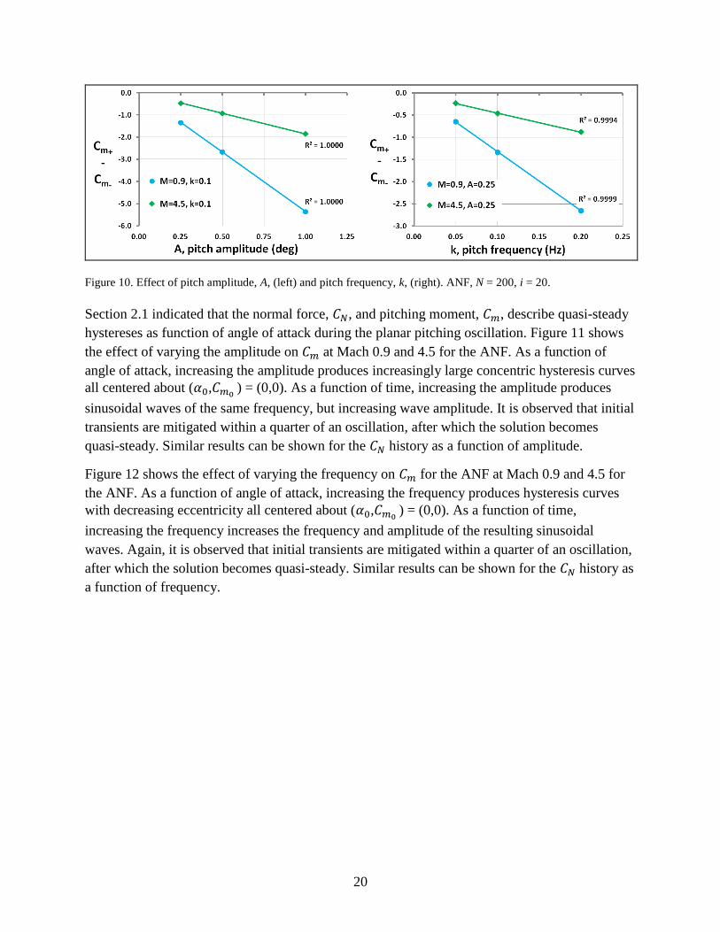
4.2.3 Amplitude and Frequency Dependence ............................................................19
4.3 Steady Lunar Coning Parameter Study for ANF...........................................................22
4.3.1 General Trend, Grid Dependence, Effect of Fin Cant and Magnus Effect .......22
4.3.2 Coning Rate and Coning Angle Dependence ....................................................24
4.4 Final Pitch Damping Results for ANF and AFF: Comparing Planar Pitching and Lunar
Coning Methods .....................................................................................................................26
5. Conclusion 30
6. References 33
Appendix. CFD Pitch Damping Data 37
List of Symbols, Abbreviations, and Acronyms 39
Distribution List 42
v
List of Figures
Figure 1. Sample pitching moment history as a function of angle of attack for α0 = 30°. ...............5
Figure 2. ANF (27), dimensions in calibers, one caliber = 0.03 m. .................................................9
Figure 3. AFF (28), dimensions in calibers, one caliber = 0.03 m. .................................................9
Figure 4. Computational grids ( = 0°) for ANF (left) and AFF (right): (a–b) whole grid on symmetry plane, (c–d) nearfield grid on symmetry plane and on projectile surface, and (e–f) grid detail between fins. ..................................................................................................11
Figure 5. Static coefficient prediction at zero angle of attack as a function of Mach number for the ANF (left) and AFF (right). Shown here are axial force ( ), normal force derivative ( ), and pitching moment derivative ( ) coefficients at zero angle of attack. .......................................................................................................................................15
Figure 6. Mach number numerical flowfield on x-z symmetry plane for the ANF (left) and AFF (right). Results are from steady-state static simulations at = 0. ...................................16
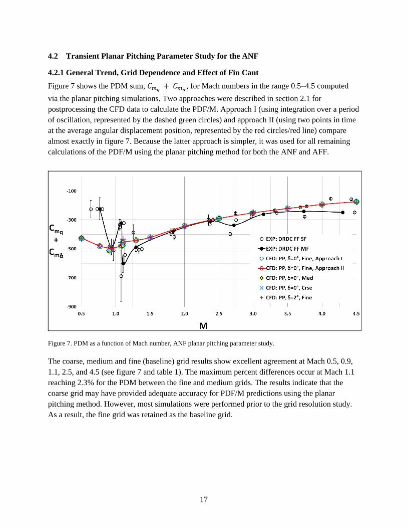
Figure 7. PDM as a function of Mach number, ANF planar pitching parameter study.................17
Figure 8. Effect of inner iterations on PDM at Mach 0.9 (left) and Mach 4.5 (right). ANF, A=0.25°, k=0.1. ........................................................................................................................19
Figure 9. Effect of global iterations per cycle on PDM at Mach 0.9 (left) and Mach 4.5 (right). ANF, A=0.25°, k=0.1. ..................................................................................................19
Figure 10. Effect of pitch amplitude, A, (left) and pitch frequency, k, (right). ANF, N = 200, i = 20. .........................................................................................................................................20
Figure 11. Effect of pitch amplitude, A, on pitching moment, , as a function of angle of attack, α, (left) and time, t, (right). ANF, k = 0.1, N = 200, i = 20. .........................................21
Figure 12. Effect of reduced pitch frequency, k, on pitching moment, , as a function of angle of attack, α, (left) and time, t, (right). ANF, A = 0.25, N = 200, i = 20. .........................22
Figure 13. PDM as a function of Mach number – ANF lunar coning parameter study.................23
Figure 14. Variation of side moment, , with coning rate, , for the ANF, = 0°. ...................25
Figure 15. Variation of side moment slope, , with sine of the coning angle, , for the ANF..........................................................................................................................................26
Figure 16. PDM sum variation with Mach number for ANF. .......................................................27
Figure 17. PDF sum variation with Mach number for ANF. .........................................................28
Figure 18. PDM sum variation with Mach number for AFF. ........................................................29
Figure 19. PDF sum variation with Mach number for AFF. .........................................................30

vi
List of Tables
Table 1. Planar pitching predictions: percent differences between grid levels for ANF. ..............18
Table 2. Lunar coning predictions: percent differences between fine, medium and coarse grid for ANF. ...................................................................................................................................24
Table A-1. CFD results – pitch damping vs. Mach number, Army-Navy basic finner (fine grid). .........................................................................................................................................38
Table A-2. CFD results – pitch damping vs. Mach number, Air Force modified finner. ..............38

vii
Acknowledgments
The authors would like to thank Dr. James DeSpirito and Dr. Paul Weinacht of the U.S. Army
Research Laboratory (ARL) at Aberdeen Proving Ground, MD, for their technical guidance on
the subject matter. This work was supported in part by a grant of high-performance computing
time from the U.S. DOD High Performance Computing Modernization Program (HPCMP) at the
Army Research Laboratory DOD Supercomputing Resource Center (ARL DSRC) at Aberdeen
Proving Ground, Maryland.

viii
INTENTIONALLY LEFT BLANK.

1
1. Introduction
Aerodynamic prediction of dynamic stability derivatives is critical to the design of ballistic and
missile weapons. Dynamic stability derivatives are a measure of how the in-flight forces and
moments acting on a flight body change in response to changes in flight states, such as angle of
attack and velocity. The main dynamic stability derivatives are the pitch damping force, pitch
damping moment, roll damping moment, Magnus force and Magnus moment. These dynamic
stability derivatives are used to conduct flight stability analyses as projectiles undergo complex
pitch-roll-yaw motions. This ensures stable yet maneuverable airframe designs for precision
projectile munitions.
Computational fluid dynamics (CFD) is recognized as an efficient and cost-effective tool for
predicting aerodynamic forces and moments, and often complements free-flight ballistic range
tests, wind-tunnel experiments, and semi-empirical analytical estimation. In this study,
Reynolds-Averaged Navier−Stokes (RANS) CFD techniques and linear flight mechanics theory
were used to compute the pitch damping force (PDF) and pitch damping moment (PDM) for a
finned projectile using two methods, viz, the “transient planar pitching” method (1−11), and the
“steady lunar coning” method (12–21). Most studies have independently used these two methods,
but the methods were not directly compared, and were mostly applied to supersonic flight.
DeSpirito et al (11) applied both methods to an axisymmetric spinner rocket, but not to a finned
projectile. This study presents the first combined application of these methods for finned
projectiles in which these methods were quantitatively assessed and directly compared for
accuracy and efficiency in predicting the pitch damping dynamic stability derivatives across the
full Mach number regime, viz, subsonic, transonic and supersonic. Detailed investigations were
conducted for each method to determine modeling sensitivities and limitations with respect to
numerical and aerodynamic modeling parameters. These included the effect of fin cant and
computational grid density on the numerical solutions.
Transient planar pitching (PP), for the purpose of this study, is the motion whereby the projectile
harmonically oscillates about its center of gravity in rectilinear flight. This is numerically
achieved via a forced sinusoidal motion. This motion is time-dependent, and therefore time-
accurate CFD methods were used to compute the flow solution. Linear mechanics theory relates
the pitch damping force and moment (PDF/M) to the normal force and pitching moment as the
projectile oscillates, allowing the PDF/M to be calculated (22–24). In addition to the effect of fin
cant and grid density, investigations included dependence on the timestep and inner iterations of
the RANS time integration scheme, and dependence on the oscillation amplitude and frequency.
Steady lunar coning (LC) is the motion whereby the projectile flies at a constant angle with
respect to the freestream velocity vector while undergoing a constant angular rotation about a
line parallel to the freestream velocity vector and passing through the projectile’s center of

2
gravity. This coning motion is comprised of two time-dependent orthogonal pitching motions
plus a time-dependent spinning motion. However, the combination of these motions is time-
independent, allowing the use of steady-state (SS) CFD methods to compute the flow solution
(20). Linear mechanics theory (15, 19) relates the PDF/M to the side force and moment, side
force, and moment angle of attack derivatives, and the Magnus force and moment derivatives
during the coning motion, allowing the PDF/M to be calculated. Previous studies have assumed
the Magnus force and moment to be negligible for finned projectiles undergoing lunar coning
motion (16, 20) resulting in approximated pitch damping solutions. This study computed the
Magnus components of lunar coning via separate transient axial roll simulations to theoretically
obtain more accurate pitch damping force and moment predictions. In addition to the effect of fin
cant and grid density, investigations included dependence on the coning rate and coning angle.
The projectile flowfields for the prescribed dynamic motions were computed using CFD++ (25),
a commercial fluid flow solver by Metacomp Technologies. The three-dimensional,
compressible RANS equations of fluid dynamics were solved, from which the aerodynamic
forces, moments and stability derivatives were calculated.
The computations were performed for two basic finned projectiles, viz, the Army-Navy Basic
Finner (ANF) and the Air Force Modified Finner (AFF). These projectiles have been used as
reference projectiles for many years and have been extensively tested in aeroballistic free-flight
ranges and wind tunnels (26–29). Data were obtained for validation of CFD results from
experiments conducted at Defense Research and Development Canada (DRDC) Valcartier
Aeroballistic Range and Trisonic Wind-Tunnel Facilities (26–28) in Quebec, Canada, and the
U.S. Air Force Research Laboratory (AFRL) Aeroballistic Research Facility (ARF) (29) at Eglin
Air Force Base in Florida.
2. Theoretical Basis
The total forces and moments acting on the projectile with respect to (w.r.t.) the projectile-fixed
coordinate reference frame were obtained from the RANS solution. These total forces and
moments were nondimensionalized using freestream density, freestream velocity, and a reference
area—the cross-sectional area of the projectile at the center of gravity location—to obtain the
total force and moment coefficients (standard aerodynamic procedures). The data were then
manipulated using linear flight mechanics theory to compute the PDF/M dynamic stability
derivatives, defined as (22–23)
(1)

3
where and are the pitch rate and angle of attack rate (also called the plunge rate),
respectively. and are pitch and plunge derivative coefficients, respectively. Because it is
usually difficult to experimentally and numerically compute the individual components and
, the coefficient sum
is instead computed; this is consistent with current practice.
The terms “PDF/M” and “PDF/M sum” are therefore used interchangeably in the remainder of
this report.
The pitch damping force is often small in comparison to the pitch damping moment and is
therefore often neglected. In fact, there were no pitch damping force experimental data to
compare to in this study. However, CFD pitch damping force results are still presented herein for
completeness. The pitch damping moment can have a significant impact on stability and should
be negative for dynamically stable flight.
The following sections describe how the PDF/M coefficients were obtained using two different
methods, viz, (1) transient planar pitching and (2) steady lunar coning. All forces and moments
were measured w.r.t. the projectile-fixed coordinate system whose x-axis is positive “nose-to-
tail,” z-axis is positive “up” and whose origin is at the center of gravity of the projectile.
2.1 Transient Planar Pitching Method
Transient planar pitching (also referred to as the forced planar pitching or forced oscillation
method) is the motion whereby the projectile harmonically oscillates about its center of gravity
in rectilinear flight. This motion is time-dependent and requires time-accurate/unsteady RANS to
numerically compute the flow solution. For this motion, first-order Taylor series expansion of in-
plane forces and moments, represented by as a function of time, , results in (22–24)
(2)
where is the zero-angle of attack static coefficient and is the angle of attack derivative
coefficient.
Forced planar pitching is numerically achieved by imposing a small-amplitude oscillation about
a mean angle of attack, , defined by the sinusoidal function
(3)
where A is the amplitude of the pitching motion (typically <1°), is the angular velocity, and
is the pitch angle relative to the body-fixed reference frame at time t. For this study, the PDF/M
were computed at zero angle of attack, therefore =0. For forced planar pitching, the pitch rate
and angle of attack rate are equal, that is
(4)
4
For simplification, and consistency with current literature, a reduced pitch frequency, k, is
defined as
(5)
The PDF/M can be calculated via two approaches as described below.
2.1.1 Approach I: Integrating Over a Period of Oscillation
This approach is more generalized and has been used by Park et al. (6, 7) and McGowan et al.
(3), among others. For small amplitude oscillation, the PDF/M can be assumed constant.
Integrating equation 2 w.r.t. , and combining with equation 4, yields
(6)
The integrals of and over one period of motion is zero, and equation 6 simplifies to
(7)
Substituting equations 3 and 5 into equation 7, the following is obtained for the PDF/M
(8)
The variation of with time over a period of oscillation is obtained from the RANS simulation,
and the integral in equation 8 can be solved using the trapezoidal rule, as follows:
(9)
where
(10)
and N is the number of numerical timesteps per period of oscillation used for solving the RANS
equations.
2.1.2 Approach II: Solving at the Mean Angular Displacement Position
This approach has been used by Sahu (8), DeSpirito et al. (11) and Bhagwandin et al. (1, 2),
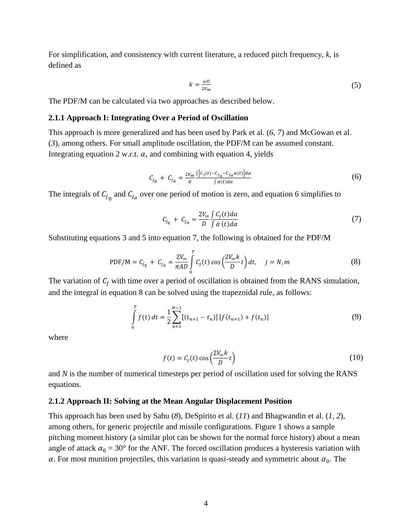
among others, for generic projectile and missile configurations. Figure 1 shows a sample
pitching moment history (a similar plot can be shown for the normal force history) about a mean
angle of attack = 30° for the ANF. The forced oscillation produces a hysteresis variation with
. For most munition projectiles, this variation is quasi-steady and symmetric about . The

5
PDF/M can thus be computed using just the two points during an oscillation where the projectile
passes through . Let the subscripts “+” and “–“ represent the pitch-up and pitch-down motions,
respectively. Then, evaluating equations 2–5 at = results in
(11)
where n represents every half oscillation, and is the value of when = . equation 11 can
be used to calculate the PDF/M, where and can be determined via a steady-state static
RANS solution at = . However, the symmetric nature of the pitch-up and pitch-down motions
leads to the following simplification:
Figure 1. Sample pitching moment history as a
function of angle of attack for α0 = 30°.
For the planar pitching motion, the nominal chosen pitch amplitude, A, was 0.25° and reduced
pitch frequency, k, was 0.1. The formulations in both approaches imply that the normal force and
pitching moment must vary linearly with and . This linear dependence was investigated at
sample Mach numbers of 0.9 and 4.5, the results of which are presented in section 4.2.3. The
pitch frequency, , and period of oscillation, , can be calculated from
The nominal number of integration timesteps per oscillation, N, used to solve the RANS
equations was 200. The numerical integration timestep, , (also referred to as the global or
physical timestep) was therefore determined as
(12)
(13)

6
Several values of N were tested to determine its effect on numerical convergence, the results of
which are presented in section4.2.2.
2.2 Steady Lunar Coning Method
Murphy (24), Schiff (15, 16), Tobak and Schiff (17, 18) and Tobak et al (19) have theoretically
examined the aerodynamics of bodies undergoing coning motion. Weinacht et al (20–21), among
others, later applied Navier−Stokes numerical techniques to solve the flowfield of projectiles
undergoing coning motion in order to calculate the PDF/M. For the purpose of this study, steady
coning is the motion whereby the projectile flies at a constant angle, , with respect to the
freestream velocity vector while undergoing a constant angular rotation, about a line parallel to
the freestream velocity vector and passing through the projectile’s center of gravity. In this case,
is therefore the total angle of attack, that is, the magnitude of the vector sum of the vertical and
horizontal angles of attack. This coning motion is a comprised of two time-dependent orthogonal
pitching motions plus a time-dependent spinning motion. However, the combination of these
motions is time-independent, allowing the use of steady-state RANS to numerically compute the
flow solution (20). For this coning motion, as derived from the general case of arbitrary motion
(14), the side moment, , is related to the Magnus moment derivative, , pitch damping
moment sum, , and the side moment angle of attack derivative,
, as follows (20–
21):
(15)
A nondimensional angular coning rate, , can be defined as
(16)
From equations 15 and 16, for linear variations of with
(17)
For small coning angles, . Therefore, from equation 17, the PDM coefficient sum
can be expressed as
(18)
(14)

7
As stated, equation 17 assumes that varies linearly with . To satisfy this linear assumption,
several coning rates were tested for select Mach numbers, the results of which are presented in
section 4.3.2. For a symmetric finned projectile without fin cants or bevels, when ,
and only a single coning computation at some nonzero within the linear range is required to
compute . For a finned projectile with fin cants or bevels, since , then simulations
at two independent coning rates (which may include zero coning rate) are required to determine
(20).
The formulation in equation 18 also indicates that the PDM is independent of the coning angle
for linear variations of with . The limits of this linear dependence were
investigated using several coning angles at select Mach numbers, the results of which are also
presented in section 4.3.2. The side force, , due to the coning motion can also be derived from
the general case of arbitrary motion as (20–21)
(19)
By similar deduction, the PDF coefficient sum can be derived as
(20)
2.2.1 Transient Roll
The Magnus force and moment that arises during coning results from unequal fluid pressures on
opposite sides of the projectile body. The Magnus force and moment derivatives, and
,
cannot be determined directly from the coning simulation. Because the Magnus effect arises only
from the spin component of the coning motion, then a separate “transient rolling” simulation was
performed. Rolling, in this case, is the motion whereby the projectile flies at a constant angle, ,
with respect to the freestream vector while rotating about its body-fixed -axis with constant
angular velocity, . This time-dependent spinning motion is intended to replicate the spin
component of the coning motion. Therefore, the rolling motion was executed such that (20)
(21)
(22)
This method is not discussed or investigated in as much detail as the previous methods. It is only
used to quantify the Magnus effect during coning. A future study will utilize this method to
compute the roll damping stability derivatives and Magnus effect, where more detailed
investigations will be provided.

8
For the rolling simulations, the projectile was spun for two full rotations completing 720° using a
nominal N = 1440 numerical timesteps per rotation [based on tested values in references (8, 30)],
equivalent to spinning the projectile 0.25° every timestep. The timestep, , was therefore
computed as
(23)
where T is the period of rotation. The side force and moment, and , were then averaged
from the final rotation. Assuming a linear variation of and with and , then the Magnus
force and moment derivatives, and
, were computed as
(24)
(25)
where and are the side force and moment, respectively, at zero spin rate and are mainly
due to fin cants/bevels. and were computed via separate steady-state RANS simulations.
The Magnus force and moment computed via equations 24 and 25 should be the equivalent
Magnus force and moment generated during the coning motion, and are thus substituted into
equations 20 and 18, respectively.
3. Geometry and Computational Methodology
3.1 Projectile Configurations and Experimental Data
Two finned projectiles were used as test models, viz, the ANF and the AFF. Figure 2 shows the
geometry details of the ANF. The ANF had a diameter of 0.03 m (1 caliber), and consisted of a
10° cone that was 2.84 calibers long, followed by a 7.16 caliber cylindrical body. There were
four 1 × 1 caliber fins with sharp leading edges and thicknesses of 0.08 calibers at the trailing
edge. CFD data for fin cants of = 0° (baseline case) and = 2° were used for comparison with
experiment. The center of gravity of the ANF was located 5.5 calibers from the nose tip. The
mass of the model was 1.5894 kg. The axial and transverse moments of inertia were 1.924 × 10⁻⁴
kg∙m2 and 9.874 × 10
-3 kg∙m
2, respectively.

9
Figure 2. ANF (27), dimensions in calibers, one caliber = 0.03 m.
Figure 3 shows the geometry details of the AFF. The AFF also had a diameter of 0.03 m (one
caliber) and consisted of tangent ogive nose that was 2.5 calibers long followed by 7.5 caliber
cylindrical body. There were four clipped-delta fins with sharp leading and trailing edges.
Although canted fin data were available, only the 0° fin cant experimental data were used for
comparison with CFD. The center of gravity of the AFF was located 4.8 calibers from the nose
tip. The mass of the model was 0.6643 kg. The axial and transverse moments of inertia were
7.197 × 10⁻⁴
kg∙m2 and 4.857 × 10
-3 kg∙m
2, respectively.
Figure 3. AFF (28), dimensions in calibers, one caliber = 0.03 m.
For comparison with CFD results, experimental data for both the ANF and AFF were obtained
mainly from free-flight (FF) tests conducted at DRDC-Valcartier Aeroballistic Range (26–28).
Nominal pressure and temperature flight conditions were PS = 01325 Pa and TS = 293.15 K,
respectively. Test Mach numbers ranged from 0.5–4.5 for the ANF and 0.5–2.5 for the AFF. The
Reynolds number, based on projectile length, ranged from 4.1 × 10⁶ to 30.0 × 10
6. Models with
fin cants of = 0, 2, and 4° were also tested. The aerodynamic coefficients were reduced from
the free-flight trajectory data (time, position, and orientation) using fixed-plane, six-degree-of-
freedom (6-DOF) numerical integration analysis. Single-fit (SF) and multiple-fit (MF) data sets
were obtained. The MF procedure simultaneously fits several flight data sets, including multiple
fin cants, to a common set of aerodynamics to theoretically produce more

10
accurate aerodynamic coefficients. The quoted Mach number for each data set was the midrange
Mach number for the SF data, and the average midrange Mach number for the multiple-fit data.
For the moment aerodynamic coefficients, the moment reference center was located at the center
of gravity of the projectile.
Additional static aerodynamic data for the ANF were also obtained from DRDC wind-tunnel
(WT) tests (27). The wind-tunnel Reynolds number ranged from 1.4 × 10
6 to 2.9 × 10
6 for Mach
numbers in the range 0.5–4.5. The static aerodynamic coefficients were obtained by least-square
fitted polynomials through measured experimental data.
Additional experimental data for the AFF were obtained from free-flight tests conducted by
AFRL ARF (29). The test model in this case was a scaled down version of the one used in the
DRDC tests. The diameter of this model was 0.01905 m. The model was launched at
atmospheric conditions similar to that of the DRDC tests at Mach numbers in the range 0.6–2.5.
SF and MF aerodynamic coefficients were obtained by a similar reduction process as that used in
the DRDC tests.
3.2 Computational Domains and Boundary Conditions
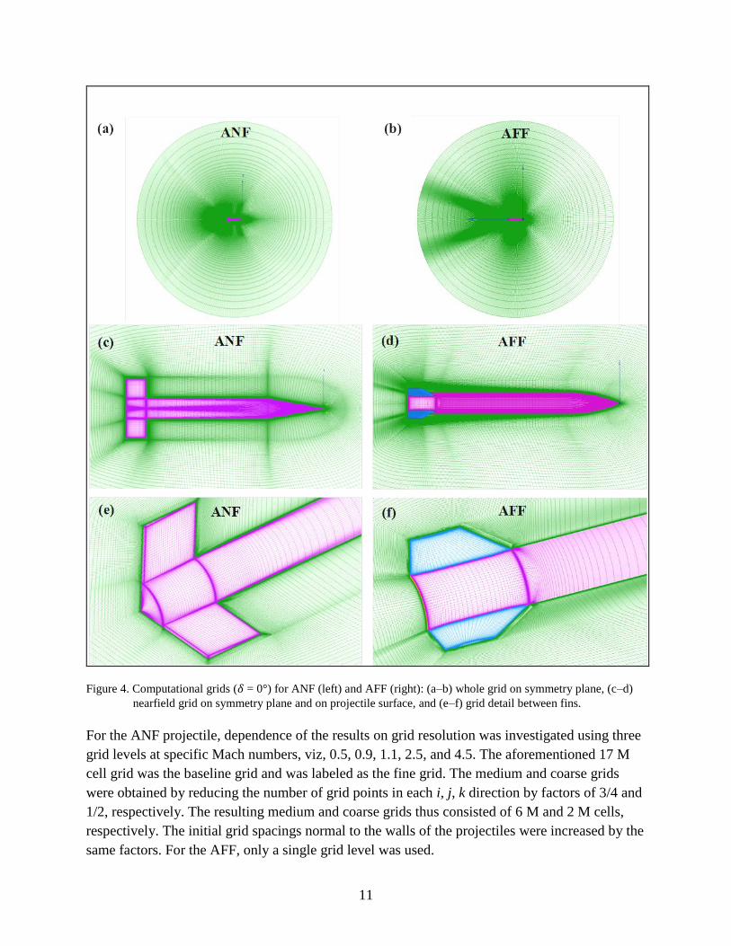
The baseline 0° fin cant computational grids for the ANF and AFF consisted of 17 and 15 M
structured hexahedral cells, respectively, both constructed in Pointwise V16.03R4 (31) and both
exported in double precision format (see figure 4). The grids were extended ~60 calibers in the
radial direction to form spherical farfield boundaries, where a characteristics-based
inflow/outflow boundary condition was applied. The first two cell layers from the farfield
boundaries was set as absorbing layers, where a damping source term was added in CFD++ to
prevent possible numerical wave reflections which may contaminate the flow solution. The
projectile walls were designated viscous adiabatic walls and utilized a solve-to-the-wall strategy
where the initial grid spacing normal to the walls was 0.0005 mm, satisfying the y+ ≤ 1 criteria
for adequate boundary-layer resolution across all Mach numbers. A 20% stretching factor was
used between successive grid points off the projectile walls. The 2° fin cant grid for the ANF
was the same as that of the 0° fin cant grid, except for minor modifications near the fins to
accommodate the fin cants.
11
Figure 4. Computational grids ( = 0°) for ANF (left) and AFF (right): (a–b) whole grid on symmetry plane, (c–d)
nearfield grid on symmetry plane and on projectile surface, and (e–f) grid detail between fins.
For the ANF projectile, dependence of the results on grid resolution was investigated using three
grid levels at specific Mach numbers, viz, 0.5, 0.9, 1.1, 2.5, and 4.5. The aforementioned 17 M
cell grid was the baseline grid and was labeled as the fine grid. The medium and coarse grids
were obtained by reducing the number of grid points in each i, j, k direction by factors of 3/4 and
1/2, respectively. The resulting medium and coarse grids thus consisted of 6 M and 2 M cells,
respectively. The initial grid spacings normal to the walls of the projectiles were increased by the
same factors. For the AFF, only a single grid level was used.

12
The ANF and AFF grids were decomposed to facilitate parallel computation on 120 and 96
processors, respectively. The computations were performed on “Harold” – a SGI Altix ICE 8200
supercomputer consisting of 1344 compute nodes, 2 quad-core Intel Xeon Nehalems per node,
24 GB memory per node, and 4X DDR Infiniband interconnect. Harold is housed and managed
by the ARL DOD Supercomputing Resource Center (ARL DSRC) at Aberdeen Proving Ground,
Maryland.
3.3 Numerics
The flow solution at a given flight condition was computed using CFD++ v10.1 (25), a
commercial CFD solver by Metacomp Technologies, Inc. CFD++ is a finite volume,
unstructured solver capable of a wide range of aerospace applications and extensively used by
ARL for projectile aerodynamic design and analysis. In this study, CFD++ was used to
numerically solve the three-dimensional, compressible, RANS equations in order to compute the
total aerodynamic forces and moments acting on the projectile, from which the static and pitch
damping derivative coefficients were calculated. Double precision format was used for all
computations. The following sections first describe general numerical attributes for the steady-
state and time-accurate simulations, followed by a summary of the planar pitching, lunar coning,
and rolling simulation procedures.
3.3.1 Steady-State Simulations
For all steady-state RANS simulations, the solution was advanced towards steady-state
convergence using a point-implicit time integration scheme with local time-stepping, defined by
the Courant−Friedrichs−Lewy (CFL) number. A linear ramping schedule was used to gradually
increase the CFL over the first few hundred iterations, after which a constant CFL was
maintained until convergence. The maximum CFL was usually between 10 and 100, depending
on the freestream Mach number. The multigrid W-cycle method with a maximum of four cycles
and a maximum of 20 coarse grid levels was used to accelerate convergence. Implicit temporal
smoothing was applied for increased stability.
The spatial discretization function was a second-order, upwind scheme using a Harten−Lax−van
Leer−Contact (HLLC) Riemann solver utilizing Metacomp’s multi-dimensional Total-Variation-
Diminishing (TVD) flux limiter. For freestream Mach numbers 1.5 and above, first-order spatial
discretization was used for the first few hundred iterations, after which blending to second-order
occurred over the next 100 iterations, and thereafter remained fully second-order.
The turbulence model employed was Metacomp’s realizable k-ε model (25, 32), which solves
transport equations in conservative form for the turbulent kinetic energy (k) and turbulent
dissipation rate (ε). The freestream turbulence intensity was set at 2% and the turbulent-to-
laminar viscosity ratio at 50. Metacomp’s wall-bounded compressibility correction was applied
to realize diffusive mixing in the turbulent regions that would otherwise be underpredicted in
compressible flows.
13
Reductions of five orders or more of the magnitudes of the cell-averaged residuals of the RANS
equations were typically achieved within a few hundred iterations (for lower Mach numbers) to a
few thousand iterations (for higher Mach numbers). However, the total force and moment
coefficients converged relatively faster, usually within a few hundred iterations. Some cases did
demonstrate relatively small pseudo-steady oscillations in the total aerodynamic coefficients.
Therefore, for all steady-state cases, the coefficients were averaged over the final 100–200
iterations.
3.3.2 Time-Accurate Simulations
For the time-accurate/unsteady RANS simulations, the dual-time step method was employed
with the point-implicit time integration scheme, utilizing an outer/physical/global timestep and
an inner timestep. The inner timestep is a local nonphysical timestep used to converge the RANS
equations at each physical timestep. For the inner iterations, the multigrid W-cycle method and
implicit temporal smoothing was applied. Nominally, i = 20 inner timesteps were used for the
time-accurate simulations, usually resulting in 0.5–1 order of magnitude reduction in the cell-
averaged “inner” residuals of the RANS equations. Other values were tested for convergence, the
results of which are presented in section 4. The spatial discretization scheme and turbulence
model used in the time-accurate simulations were the same as that used in the steady-state
simulations.
3.3.3 Transient Planar Pitching Procedure
First, a static steady-state solution at a given Mach number was generated at an angle of attack
= = 0°. This steady-state solution was then used as the initial condition for the time-accurate
planar pitching simulation. The planar pitching oscillation was defined by the sinusoidal function
in equation 3 about a mean angle of attack = 0° with a chosen nominal amplitude and reduced
frequency of A = 0.25° and k = 0.1, respectively. A total of three oscillations/pitch cycles were
run with a nominal N = 200 timesteps per oscillation. Initial numerical transients were typically
mitigated well within the first oscillation, after which a quasi-steady cyclical convergence of the in-
plane total forces and moments was obtained. The histories of the total normal force and pitching
moment coefficients, and , for the final two oscillations were used to determine the PDF/M
using equation 8 for approach I, and equation 12 for approach II, respectively (see section 2.1).
3.3.4 Steady-State Lunar Coning Procedure
With the velocity vector parallel to the inertial x-axis, the projectile (and grid) was rotated to the
nominal coning angle = 0.5°. The projectile was then made to rotate about an axis parallel to
the velocity vector and passing through the projectile’s center of gravity at a constant angular
velocity, , calculated based on a chosen nominal nondimensional coning rate of = 0.0025.
The steady-state converged values of the total side force and moment coefficients, and ,
were then used to compute the PDF/M via equations 20 and 18, respectively. For the 2° canted

14
fin ANF, the side force and moment -derivative coefficients, and , were calculated from
steady-static simulations at = 0° and 0.5°. The Magnus terms in these equations were obtained
from the transient rolling simulations, described below.
3.3.5 Transient Rolling Procedure
The objective of the rolling simulations was to obtain the equivalent Magnus force and moment
acting on the projectile due to the spin component of the coning motion. Because the nominal
coning angle was = 0.5°, the steady-state static solution at = 0.5° was thus used as the initial
condition for the transient rolling simulations. For the rolling simulations, the projectile was
made to rotate about its body-fixed x-axis at angle of attack, , w.r.t. the freestream velocity
vector with constant angular velocity, , such that equations 21 and 22 were satisfied. The
projectile was spun for two rotations completing 720° or 4πc. Initial numerical transients were
typically mitigated well within the first rotation. The total side force and moment coefficients,
and , were averaged over the final rotation. The Magnus force and moment coefficients,
and , were then computed via equations 24 and 25, respectively. For the 2° canted fin ANF,
the zero-spin side force and moment coefficients, and , were obtained from the steady-
state static simulations at = 0.5°.
4. Results
Section 4.1 briefly presents results for prediction of static aerodynamic coefficients for the ANF
and AFF. Sections 4.2 and 4.3 show the dependence of the planar pitching and lunar coning
methods, respectively, on various numerical and physical modeling parameters. These
parametric studies were conducted only on the ANF and only for the PDM. The PDF is often
ignored in aerodynamic analyses since it does not affect flight stability. In fact, there were no
experimental data to compare to for the PDF. For these reasons, all PDF results are deferred to
section 4.4. Section 4.4 finally compares the planar pitching and lunar coning methods for both
the ANF and AFF.
4.1 Steady-state Static Results for ANF and AFF
Figure 5 compares the static aerodynamic coefficients, viz, the axial force, normal force slope,
and pitching moment slope coefficients at zero angle of attack, that is, , and
, for
Mach numbers in the range 0.5–4.5. and were calculated using a linear fit between
steady-state static solutions at 0 and 1° angles of attack. This is consistent with current practice
because these coefficients tend to vary linearly at low angles of attack. Although these
coefficients were not required for computing the pitch damping coefficients, they serve as a
check of accuracy of the static steady-state RANS solutions, which were used as initial
conditions for the dynamic time-accurate simulations. The CFD numerical data generally show

15
excellent agreement with free-flight and wind-tunnel tests across the full Mach number regime;
for the ANF the agreement is slightly better with the free-flight data than with the wind-tunnel
data at some Mach numbers. CFD data for the 2° canted fin ANF are also shown. There is no
significant difference between the canted and uncanted results. This is expected because these
coefficients do not typically vary with fin cant.
Figure 5. Static coefficient prediction at zero angle of attack as a function of Mach number for the ANF (left) and
AFF (right). Shown here are axial force ( ), normal force derivative ( ), and pitching moment
derivative ( ) coefficients at zero angle of attack.
ANF AFF

16
The experimental data for the AFF, however, show much scatter. The DRDC standard
deviation errors for this coefficient were much higher than that of the other coefficients.
Supersonically, although the DRDC single-fit and AFRL multiple-fit data match reasonably
well, the DRDC multiple-fit data are predicted to be much higher at Mach 2.2. According to
DRDC, the source of this discrepancy is undetermined. The CFD data appear to pass through the
average of the experimental data points up to Mach 1.2, then slightly underpredicted between
Mach 1.2 and 2.0; then at Mach 2.0 and 2.5 there is excellent agreement with the DRDC single-
fit and AFRL multiple fit data points. Because the CFD predictions of for the AFF are in
good agreement with experiment, then this is usually an indication that the CFD predictions of
is also good. It is likely therefore that the DRDC multiple-fit data for the AFF are incorrect.
Figure 5 also compares the effect of grid resolution on static coefficient prediction for the ANF
at specific Mach numbers, viz, 0.5, 0.9, 1.1, 2.5, and 4.5. Three grid levels were compared, viz,
fine, medium, and coarse, as previously discussed. Figure 5 shows that the results are relatively
grid-independent, except for some small differences in the subsonic/transonic region for ,
where the difference reaches a maximum of 14% at Mach 0.5. Overall, the fine grid was deemed
to be adequate for grid independent solutions, and was thus retained as the baseline grid.
Figure 6 provides a synopsis of typical static steady-state flowfields for the ANF and AFF at zero
angle of attack. Shown are Mach number contours on the symmetry plane at representative
freestream Mach numbers of 0.9 and 2.0. Typical flow features are observed, such as the
formation of shock waves on the nose and fins and low speed flows at the base of the projectiles.
Figure 6. Mach number numerical flowfield on x-z symmetry plane for the ANF (left) and AFF (right). Results are
from steady-state static simulations at = 0.
M 0.9 M 0.9
M 2.0 M 2.0
ANF AFF
17
4.2 Transient Planar Pitching Parameter Study for the ANF
4.2.1 General Trend, Grid Dependence and Effect of Fin Cant
Figure 7 shows the PDM sum, , for Mach numbers in the range 0.5–4.5 computed
via the planar pitching simulations. Two approaches were described in section 2.1 for
postprocessing the CFD data to calculate the PDF/M. Approach I (using integration over a period
of oscillation, represented by the dashed green circles) and approach II (using two points in time
at the average angular displacement position, represented by the red circles/red line) compare
almost exactly in figure 7. Because the latter approach is simpler, it was used for all remaining
calculations of the PDF/M using the planar pitching method for both the ANF and AFF.
Figure 7. PDM as a function of Mach number, ANF planar pitching parameter study.
The coarse, medium and fine (baseline) grid results show excellent agreement at Mach 0.5, 0.9,
1.1, 2.5, and 4.5 (see figure 7 and table 1). The maximum percent differences occur at Mach 1.1
reaching 2.3% for the PDM between the fine and medium grids. The results indicate that the
coarse grid may have provided adequate accuracy for PDF/M predictions using the planar
pitching method. However, most simulations were performed prior to the grid resolution study.
As a result, the fine grid was retained as the baseline grid.

18
Table 1. Planar pitching predictions: percent differences between grid levels for ANF.
Mach
No.
Planar Pitching
Difference Between Fine and
Medium Grids
Difference Between Fine and
Coarse Grids
(%)
PDM
(%)
(%)
PDM
(%)
0.5 0.01 0.09 0.51 0.76
0.9 0.03 0.01 0.08 0.01
1.1 1.82 2.28 0.63 0.92
2.5 0.02 0.14 0.14 0.42
4.5 0.45 0.03 0.18 0.21
Figure 7 shows no significant difference between the canted fin ( = 2°) and uncanted fin ( =
0°) numerical results, except near Mach 1.0 where the difference reaches about 5%.
Compared to DRDC free-flight data, the PDM CFD data are about 115% larger in magnitude at
Mach 0.766 (first free-flight multiple-fit data point in figure 7). Through the transonic region,
0.9<M<1.3, there is much scatter in the free-flight data with very large standard deviation errors
in the vicinity of Mach 1.0. In this region, the CFD PDM data appear to pass through the average
of the experimental data points. The accuracy of the free-flight data in the subsonic and transonic
regions is suspect, especially when multiple experimental data sources for the AFF are compared
later in section 4.4. Additional test data would be required to determine the accuracy of the CFD
predictions in this region. Above Mach 1.3, the CFD data generally show very good agreement
with the free-flight data.
4.2.2 Inner Iteration and Timestep Dependence
The planar pitching simulations were time-dependent. As previously discussed, the dual-timestep
method was used where the physical/global timestep, , was calculated based on a chosen
N=200 timesteps per oscillation, and the inner timestep was calculated based on a chosen i = 20
inner iterations per global iteration. Figures 8 and 9 show the effect of increasing i and N,
respectively. This study was performed only for the ANF at representative freestream Mach
numbers of 0.9 and 4.5. For these cases, the amplitude and reduced frequency of the oscillations
were A = 0.25° and k = 0.1, respectively (the baseline values).
Varying i from 5–25 in increments of 5, figure 8 shows that the PDM for the Mach 0.9 solutions
readily converge by i = 10 for both N = 100 and 200. For the Mach 4.5 cases, the PDM shows an
asymptotic convergence, where for i > 15 the PDM successively decreases by only ~1%. For
consistency and accuracy, i = 20 was thus chosen as the nominal number of inner iterations at all
Mach numbers.

19
Varying N from 100–400, the PDM shows asymptotic decrease in figure 9. For i = 20, increasing
N from 200 to 400 decreased the PDM by only 1.5% at Mach 0.9 and 2% at Mach 4.5. Thus,
sacrificing only little accuracy for a large gain in computing efficiency, N = 200 was deemed a
reasonable nominal choice at all Mach numbers.
Figure 8. Effect of inner iterations on PDM at Mach 0.9 (left) and Mach 4.5 (right). ANF, A=0.25°, k=0.1.
Figure 9. Effect of global iterations per cycle on PDM at Mach 0.9 (left) and Mach 4.5 (right). ANF, A=0.25°, k=0.1.
4.2.3 Amplitude and Frequency Dependence
Figure 10 shows the “pitching moment difference,” , as a function of pitch amplitude,
A, and pitch frequency, k, for the ANF at Mach 0.9 and 4.5. The line plots are linear
approximations using least squares linear regression fits. The regression correlation coefficient,
, values are indicated on the charts and are all very nearly equal to 1, indicating excellent
linearity. According to equation 12, this implies that the PDF/M does not vary with pitch
amplitude and frequency for the range of values tested herein. Similar results can be shown for
the normal force difference, . The nominal choices of A = 0.25° and k = 0.1 used for
all other simulations clearly lie within the linear range.
20
Figure 10. Effect of pitch amplitude, A, (left) and pitch frequency, k, (right). ANF, N = 200, i = 20.
Section 2.1 indicated that the normal force, , and pitching moment, , describe quasi-steady
hystereses as function of angle of attack during the planar pitching oscillation. Figure 11 shows
the effect of varying the amplitude on at Mach 0.9 and 4.5 for the ANF. As a function of
angle of attack, increasing the amplitude produces increasingly large concentric hysteresis curves
all centered about ( , ) = (0,0). As a function of time, increasing the amplitude produces
sinusoidal waves of the same frequency, but increasing wave amplitude. It is observed that initial
transients are mitigated within a quarter of an oscillation, after which the solution becomes
quasi-steady. Similar results can be shown for the history as a function of amplitude.
Figure 12 shows the effect of varying the frequency on for the ANF at Mach 0.9 and 4.5 for
the ANF. As a function of angle of attack, increasing the frequency produces hysteresis curves
with decreasing eccentricity all centered about ( , ) = (0,0). As a function of time,
increasing the frequency increases the frequency and amplitude of the resulting sinusoidal
waves. Again, it is observed that initial transients are mitigated within a quarter of an oscillation,
after which the solution becomes quasi-steady. Similar results can be shown for the history as
a function of frequency.

21
Figure 11. Effect of pitch amplitude, A, on pitching moment, , as a function of angle of attack, α, (left) and time,
t, (right). ANF, k = 0.1, N = 200, i = 20.

22
Figure 12. Effect of reduced pitch frequency, k, on pitching moment, , as a function of angle of attack, α, (left)
and time, t, (right). ANF, A = 0.25, N = 200, i = 20.
The results generally show that the nominal choices of A = 0.25° and k = 0.1 provide adequate
perturbation for computing the pitching damping derivatives while still satisfying the linear
assumptions of the planar pitching method.
4.3 Steady Lunar Coning Parameter Study for ANF
4.3.1 General Trend, Grid Dependence, Effect of Fin Cant and Magnus Effect
Figure 13 shows the PDM sum, , for Mach numbers in the range 0.5–4.5 computed
via the lunar coning simulations for the ANF. Several numerical studies were conducted. The
baseline case had coning angle =0.5°, coning rate =0.0025, fin cant =0°, utilized the fine
grid, and is represented by the red circles/red line in figure 13. Compared to DRDC free-flight
data, baseline PDM values at subsonic velocities are about 102% larger in magnitude at Mach
0.766 (first free-flight multiple-fit data point). As previously discussed in section 4.2.1, the

23
source of the subsonic discrepancy is undetermined. Through the transonic region, 0.9<M<1.3,
the CFD baseline predictions agree very well with the free-flight multiple-fit data points, except
at Mach 1.105 where the free-flight multiple-fit data drops to -600. Above Mach 1.3, the CFD
data generally show good to excellent agreement with the free-flight data.
Figure 13. PDM as a function of Mach number – ANF lunar coning parameter study.
Figure 13 also shows the baseline case, but with a fin cant of = 2° ( represented by the purple
Xs). The = 2° CFD data only slightly differ from the = 0° CFD data, except near Mach 1.1
where the difference reaches ~40% and between Mach 2.5 and 3.0 where the difference reaches
~25%.
As discussed in section 2.2, the Magnus force and moment components of the lunar coning
motion in equations 18 and 20 were calculated via separate transient roll simulations. To
investigate the significance of the Magnus terms using the lunar coning method on the pitch
damping predictions, figure 13 shows the PDM for the baseline case with the Magnus moment
assumed negligible, that is, with =0 (blue circles/dashed blue line). In this case, it is
observed that the magnitude of the PDM is overpredicted by ~20% in the subsonic region (0.5 ≤
M ≤ 0.9), ~150% at M = 1.105 and ~10%–30% in the supersonic region (1.3 ≤ M ≤ 4.5). The 2°
canted fin results also show similar overpredictions of the PDM magnitude when the Magnus
moment was assumed negligible (green +s). Except at Mach 1.105, the error differences between
lunar coning with and without Magnus correction still lies within generally accepted error
margins for free-flight experimental data. However, these error differences appear to be
significantly larger for the finned projectiles studied herein than that suggested by some previous
studies for axisymmetric projectiles (11).

24
Figure 13 and table 2 show the effect of grid resolution on the PDM predictions at specific Mach
numbers of 0.5, 0.9, 1.1, 2.5, and 4.5. Note that the coarse grid (yellow squares) and medium
grid (yellow triangles) results do not have the Magnus correction, and are thus compared to the
fine grid baseline case without Magnus correction (blue circles/blue line). Except at Mach 2.5,
the maximum difference between the fine and medium grid results is 3.3%. At Mach 2.5 the
difference is 10.3%. Compromising between accuracy and computing efficiency, the fine grid
was deemed acceptable for the lunar coning simulations.
Table 2. Lunar coning predictions: percent differences between fine, medium and coarse
grid for ANF.
MACH
NO.
LUNAR CONING
Difference Between Fine &
Medium Grids
Difference Between Fine &
Coarse Grids
(%)
PDM
(%)
(%)
PDM
(%)
0.5 0.23 1.15 3.12 3.03
0.9 1.46 2.33 0.96 2.47
1.1 2.63 3.28 1.56 1.63
2.5 10.30 11.71 6.27 4.98
4.5 0.64 0.18 3.34 2.24
4.3.2 Coning Rate and Coning Angle Dependence
The formulations presented in section 2.2 assumed that the side force and moment, and ,
vary linearly with nondimensional coning rate, . To determine a suitable range of for which
this linear assumption is satisfied was varied as 0.001, 0.0025, 0.005, and 0.01. Figure 14
shows the variation of with for the uncanted ANF for Mach 0.5, 1.0, and 4.5 and nominal
coning angle = 0.5°. The solid line plots are linear approximations using least-squares linear
regression fits. For Mach 0.5 and 4.5, the regression correlation coefficient, , values are nearly
1, indicating that varies very linearly with for up to 0.01. For Mach 1.0, the solid green
line was fitted only to the first three data points at which = 0.001, 0.0025, and 0.005. This solid
green line was then extrapolated for visual comparison with a second-order polynomial
regression approximation to all four values (dashed green line). This was done to demonstrate
the nonlinear variation of with for beyond 0.005 at Mach 1.0. Similar trends can be
shown for the variation of side force, , with . Based on these results, a nominal coning rate of
=0.0025 was chosen in order to satisfy the linearity assumptions for computing the PDF/M.
Note that in figure 14, the ordinate intercepts for the three Mach numbers are approximately zero
– an intuitive outcome for a symmetric uncanted/unbeveled finner. This allows the computation
of and in equations 20 and 18 as simply and , respectively. This
also implies only a single simulation at a single coning rate within the linear range is needed to
calculate the PDF/M given by equations 18 and 20 for a given freestream Mach number. For a
canted finner, the ordinate intercept would be nonzero, and at least two simulations at two

25
different coning rates would be required to compute and In this study, for the
2° canted ANF, the second coning rate was chosen as = 0, which equates to a static steady-
state computation at a fixed angle of attack equal to the coning angle.
Figure 14. Variation of side moment, , with coning rate, , for the ANF, = 0°.
The formulation of equations 18 and 20 implied that the side force and moment coning angle
derivatives, and
, vary linearly with , where is the sine of the coning angle, that is,
. Figure 15 shows the variation of with for Mach 0.5, 1.0, and 4.5, and nominal
coning rate = 0.0025 for the uncanted ANF. The coning angle was varied as = 0.25, 0.50,
1.0, 2.0, and 3.0°. The solid line plots are linear approximations using least-squares regression
fits. For Mach 0.5 and 4.5, the R2 values are very nearly 1, indicating that
varies very
linearly with for up to 3° ( ≈ 0.0523). For Mach 1.0, the solid green line was fitted only to
the first three data points for which = 0.25, 0.50, and 1.0° (i.e., up to ≈ 0.0175). This solid
green line was then extrapolated for visual comparison with a third-order polynomial regression
approximation to all five values (dashed green line). This was done to demonstrate the
nonlinear variation of with for beyond 1.0° at Mach 1.0. Similar trends can be shown for
the variation of the side force derivative, , with . Based on these results, a nominal coning
angle of = 0.5° ( ≈0.00873) was chosen in order to satisfy the linearity assumptions for
computing the PDF/M.

26
Figure 15. Variation of side moment slope, , with sine of the coning angle, ,
for the ANF.
Based on these results, the critical Mach regime for determining coning angles and coning rates
in the linear range for the lunar coning method appears to be the transonic regime.
4.4 Final Pitch Damping Results for ANF and AFF: Comparing Planar Pitching and
Lunar Coning Methods
The pitch damping force and moment results across the full Mach number regime for the ANF
and AFF are compared below. These results were obtained using nominal modeling parameters.
For the planar pitching simulations, nominal modeling parameters were as follows: inner
timestep iterations = 20, physical timestep iterations per pitch oscillation = 200, pitch
amplitude = 0.25° and reduced pitch frequency = 0.1. For the lunar coning simulations,
nominal modeling parameters were as follows: nondimensional coning rate = 0.0025 and
coning angle = 0.5°.
Figure 16 compares the PDM between that obtained via the planar pitching and lunar coning
CFD methods and DRDC free-flight data for the ANF. The 0° fin cant CFD data are considered
first. Generally, both the planar pitching (red circles/red line) and lunar coning (blue
diamonds/blue line) methods produce comparable results, except near Mach 1.1 and at Mach 2.5
and 3.0. Subsonically, for M < 0.9, there is a ~7% difference between the two CFD methods,
however, as previously noted, both methods show a significant difference (>100%) from the
DRDC free-flight data. Transonically, at M=0.934, both CFD methods compare very well with
the multiple-fit free-flight data. At M=1.077, the lunar coning method matches the multiple-fit
free-flight data, whereas the planar pitching method produces a ~50% larger magnitude. At M =

27
1.105, none of the three data sets match. As previously stated in section 3, the source/s of the
discrepancies in the subsonic and transonic regions are undetermined, and additional free-flight
data may be needed to validate the CFD methods. In the supersonic regime, above M > 1.3, both
CFD methods generally compare very well with the free-flight data, however, there is a ~17%
and ~25% difference between the two CFD methods at Mach 2.5 and 3.0, respectively.
Figure 16. PDM sum variation with Mach number for ANF.
In the transonic regime, there is much scatter in the DRDC free-flight data with larger than
normal standard deviation errors. The fluctuations/discrepancies in the free-flight data possibly
indicate a dynamic instability. Based on a dynamic stability analysis, DRDC (26) suggested that
a Magnus dynamic instability occurs in the transonic regime (0.9 < M < 1.3) and that the 4° fin
cant models, and to a lesser extent the 2° fin cant models, were subject to this instability. Recall
that the DRDC tests included fin cants of = 0, 2, and 4°. In figure 16, the DRDC single-fit data
include all three fin cants, whereas the multiple-fit data were derived from multiple data sets that
included multiple fin cants; therefore any dynamic instabilities for the canted-fin models would
be represented in figure 16.
The 2° canted fin CFD results computed via the planar pitching (green Xs) and lunar coning
(purple +s) methods match more closely with each other than the 0° canted fin CFD results, with
the largest difference being ~10% at Mach 1.105. Except in the vicinity of Mach 1.1 and to a
much lesser extent at Mach 2.5 and 3.0, the canted and uncanted PDM results are only slightly
different.

28
Figure 17 compares the PDF between the planar pitching and lunar coning CFD methods for the
ANF. No experimental data were available for comparison. For the uncanted fin, again, the two
CFD methods (red and blue lines) are comparable, except in the vicinity of Mach 1.1 (~34%
difference) and to a lesser extent at Mach 2.5–3.0 (~17%–27% difference). Like the PDM
results, the 2° canted fin results for the two methods (green Xs and purple +s) match more
closely with each other, and, except in the vicinity of Mach 1.1, generally only slightly differ
from the uncanted fin results.
Also shown in figure 17 are lunar coning PDF predictions without the Magnus correction for the
uncanted and canted fins (pink dashed line and orange triangles, respectively). As observed in
the PDM results of figure 13, figure 17 also demonstrates that ignoring the Magnus effect results
in an overprediction of the PDF magnitude when using the lunar coning method; the difference is
~5% in the subsonic regime, ~117% at Mach 1.105, and ~10%–30% in the supersonic regime.
Figure 17. PDF sum variation with Mach number for ANF.
Figure 18 compares PDM results for the AFF obtained via the planar pitching and lunar coning
CFD methods with DRDC and AFRL free-flight experimental data. In general, the planar
pitching and lunar coning methods (red and blue lines) compare very well with each other
particularly in the subsonic regime; between Mach 1.0 and 2.0 the disagreement is more notable
where it reaches a maximum of ~30% at Mach 1.1; at Mach 2.5 the agreement is again very
good.

29
Figure 18. PDM sum variation with Mach number for AFF.
In the transonic and supersonic regimes above Mach 0.9, the AFRL data show a higher PDM
magnitude than the DRDC multiple-fit data, reaching a difference of ~30% at Mach ~1.65. In
these regimes, the lunar coning method generally matches the DRDC data better, whereas the
planar pitching method (except at Mach 1.05) generally matches the AFRL data better.
In the subsonic regime below Mach 0.9, the PDM predicted by both CFD methods is larger in
magnitude than the AFRL data, reaching a difference of ~60% at Mach 0.6. Between Mach 0.65
and 1.0, the DRDC data are grossly different from the AFRL and CFD data. In fact, the DRDC
single-fit data point at Mach ~0.7 and multiple-fit data point at Mach ~0.8 show positive pitch
damping, indicating dynamically unstable flight. According to DRDC (28), neither resonance nor
Magnus effects were responsible for the pitch damping instability. Although the cause was
therefore undetermined, it was conjectured to be damage to the test projectile, possibly on the
fins. Note that for this AFF case, two different experimental data sets, viz, DRDC and AFRL,
show very different pitch damping results in the subsonic region. The extent of the variability in
the free-flight data sets in the subsonic and low transonic regions further supports the
aforementioned conclusion that the accuracy of the CFD in this Mach number range is still
inconclusive and additional experimental data are required.
Figure 18 also shows the lunar coning PDM results without the Magnus correction (dashed green
line). As noted in results for the ANF, if the Magnus effect is ignored, the PDM magnitude is
generally overpredicted; the difference is ~12% at Mach 0.7 and ~52% at Mach 1.5. There is one
exception that occurs at Mach 0.9 where the PDM magnitude is underpredicted by ~10% without
the Magnus correction.

30
Figure 19 compares the PDF between the planar pitching and lunar coning CFD methods for the
AFF. No experimental data were available for comparison. Between Mach 0.6 and 1.0, the two
methods (red and blue lines) show significant disagreement, reaching 24% difference at Mach
0.9. Above Mach 1.0, the disagreement is much less, reaching 12% at Mach 2.5. Considering all
previous results, the disagreement in the subsonic region was higher than expected.
Figure 19. PDF sum variation with Mach number for AFF.
Also shown in figure 19 are lunar coning PDF results without the Magnus correction (dashed
green line). Above Mach 1.0, the PDF magnitude without Magnus correction is overpredicted as
expected, reaching ~12% difference at Mach 1.3. However, unlike previous trends, the PDF
magnitude without Magnus correction is underpredicted below Mach 1.0, reaching ~25%
difference at Mach 0.9. This behavior is yet to be further investigated.
5. Conclusion
RANS CFD and flight mechanics theory were used to compute the pitch damping dynamic
stability derivatives via two distinct numerical techniques, viz, the time-accurate planar pitching
method and the steady-state lunar coning method. The pitch damping force and moment were
computed across the full Mach number regime for two basic finned projectiles, viz, the ANF and
the AFF. Solution dependence on several aerodynamic and numerical modeling parameters was
investigated. Numerical results, where available, were compared against free-
31
flight aeroballistic range data, as well as some wind-tunnel data, from Defense Research and
Development Canada Valcartier Aeroballistic Range and Trisonic Wind-Tunnel Facilities in
Quebec, Canada, and the U.S. AFRL ARF at Eglin Air Force Base, Florida.
For the planar pitching method, the pitch damping derivatives were shown to be related to the
normal force and pitching moment for forced sinusoidal oscillation of the projectile. The pitch
damping predictions were demonstrated to be fairly independent of the pitch amplitude and pitch
frequency for linear variations of the normal force and pitching moment with amplitude and
frequency. These linear variations were shown for amplitudes up to 1° and nondimensional
frequencies up to 0.2 for the Army−Navy Finner. The limits of these linear variations will
depend on projectile geometry and flight conditions, such as Mach number. The quasi-steady
hysteresis variation of the normal force and pitching moment with angle of attack during the
planar pitching motion was also demonstrated. The accuracy of the pitch damping predictions
depended on the choices of physical timestep and inner iterations of the dual-timestep integration
scheme used for solving the RANS equations. It was observed that the sensitivity of this
dependence increases at higher freestream Mach numbers. Two hundred physical iterations per
pitch cycle and twenty inner iterations were deemed sufficient for the computations herein,
sacrificing only little accuracy for significant increases in computational efficiency. The
Army−Navy Finner 2° fin cant appeared to have little or no effect on the pitch damping
predictions computed via planar pitching. There was also little sensitivity of the planar pitching
results to the three grid sizes tested herein for the Army−Navy Finner.
For the lunar coning method, the pitch damping derivatives were shown to be related to the total
side force and moment, Magnus force and moment, and in the case of canted fins, to the side
force and moment angle of attack derivatives. The pitch damping predictions were demonstrated
to be independent of the coning angle and coning rate for linear variations of the side force and
moment with coning rate and coning angle. These linear variations were investigated for coning
angles up to 3° and nondimensional coning rates up to 0.01 for the Army−Navy Finner. The
linear assumptions degenerated at smaller coning angles and coning rates for the transonic Mach
regime than for the subsonic and supersonic regimes. The Magnus effect as a result of the lunar
coning motion on the pitch damping predictions was shown to be significant for both finned
projectiles, particularly in the transonic Mach regime. Assuming the Magnus effect to be
negligible usually resulted in an overprediction of the pitch damping force and moment
magnitudes, except for the pitch damping force for the Air Force Finner below Mach 1.0. The
Magnus terms were determined via separate time-dependent axial roll simulations. Since no
parametric studies were conducted for the latter, the accuracy of the Magnus computations is yet
to be verified – an exercise left for a future study. The Army−Navy Finner 2° fin cant appeared
to have little effect on the pitch damping predictions computed via lunar coning, except in the
transonic regime where the difference was more notable. Except at one supersonic Mach number,
the lunar coning results were shown to be fairly grid-independent of the three grid levels tested.

32
Generally, the two numerical techniques—planar pitching and lunar coning—yielded fairly
comparable results across most of the Mach number range. The largest differences between the
two techniques occurred in the transonic regime, particularly for the Army−Navy Finner.
Compared to free-flight test data, both techniques generally show good agreement in the high
transonic and supersonic regimes, but poor agreement in the subsonic and low transonic regimes.
In the subsonic and low transonic regimes, the accuracy of the free-flight test data was uncertain
due to instances of large scatter, large standard deviation errors and different data sources
showing significantly different results. The variability of the free-flight data therefore
necessitates additional experimental data to validate the numerical methods.
Regarding computational effort, the planar pitching method requires only a single time-accurate
oscillatory computation, whereas the lunar coning method requires a steady-state coning
computation plus a time-accurate rolling computation to account for the Magnus effect. Because
the Magnus effect during coning can be significant even for a finned projectile, the planar
pitching method offers a more efficient method of computing the pitch damping derivatives than
the lunar coning method. Also, the Magnus effect can be difficult to compute accurately for
some projectiles at subsonic and transonic speeds—a source of error that the planar pitching
method does not inherit. However, if full aerodynamic characterization of a projectile is needed,
the time-accurate rolling computations would have to be conducted regardless to compute the
roll damping and Magnus derivatives, in which case either planar pitching or lunar coning to
compute the pitch damping derivatives may equally suffice.

33
6. References
1. Bhagwandin, V. A; Sahu, J. Numerical Prediction of Pitch Damping Derivatives for a Finned
Projectile at Angles of Attack. AIAA Aerospace Sciences Meeting, AIAA 2012-691,
Nashville, TN, January 2012.
2. Bhagwandin, V. A.; Sahu, J. Numerical Prediction of Pitch Damping Stability Derivatives
for Finned Projectiles. AIAA Applied Aerodynamics Conference, AIAA 2011-3028,
Honolulu, HI, June 2011.
3. McGowan, G. Z.; Kurzen, M. J.; Nance, R. P.; Carpenter, J. G.; Moore, F. G. Computational
Investigation of Pitch Damping on Missile Geometries at High Angles of Attack. AIAA
Applied Aerodynamics Conference, AIAA 2012-2903, New Orleans, LA, June 2012.
4. Murman, S. M. Reduced-Frequency Approach for Calculating Dynamic Derivatives. AIAA
Journal 2007, 45 (6), 1161–1168.
5. Oktay, E.; Akay, H. CFD Predictions Of Dynamic Derivatives for Missiles. AIAA Aerospace
Sciences Meeting, AIAA 2002-0276, Reno, NV, January 2002.
6. Park, S. H.; Kim, Y.; Kwon, J. H. Prediction of Damping Coefficients Using the Unsteady
Euler Equations. AIAA Journal of Spacecraft and Rockets May-June 2003, 40 (3), 356–362.
7. Park, S. H.; Kwon, J. H.; Kim, Y. Prediction of Dynamic Damping Coefficients Using
Unsteady Dual-Time Stepping Method. AIAA Aerospace Sciences Meeting, AIAA 2002-
0715, Reno, NV, January 2002.
8. Sahu, J. Numerical Computations of Dynamic Derivatives of a Finned Projectile Using a
Time-Accurate CFD Method. AIAA Atmospheric Flight Mechanics Conference, AIAA
2007-6581, August 2007.
9. Stalnaker, J. F.; Robinson, M. A. Computation of Stability Derivatives of Spinning Missiles
Using Unstructured Cartesian Meshes. AIAA Applied Aerodynamics Conference, AIAA
2002-2802, St. Louis, MO, June 2002.
10. Weinacht, P. Characterization of Small-Caliber Ammunition Performance Using a Virtual
Wind Tunnel Approach. AIAA Atmospheric Flight Mechanics Conference, AIAA 2007-
6579, Hilton Head, SC, August 2007.
11. DeSpirito, J.; Silton, S, I.; Weinacht, P. Navier-Stokes Predictions of Dynamic Stability
Derivatives: Evaluation of Steady-State Methods. AIAA Journal of Spacecraft and Rockets
November-December 2009, 46 (6), 1142–1154.

34
12. Agarwal, R.; Rakich, J. V. Computation of Supersonic Laminar Viscous Flow Past a Pointed
Cone at Angle of Attack in Spinning and Coning Motion. AIAA Fluid and Plasma Dynamics
Conference, AIAA 78-1211, Seattle, WA, July 1978.
13. Lin, T. C. Numerical Study of Re-entry Vehicle Aerodynamics in Steady Coning Motion.
AIAA Journal of Spacecraft and Rockets May 1981, 18 (3), 228–234.
14. Levy, L. L.; Tobak, M. Nonlinear Aerodynamics of Bodies of Revolution in Free Flight.
AIAA Journal 1970, 8 (12), 2168–2171.
15. Schiff, L. B. Nonlinear Aerodynamics of Bodies in Coning Motion. AIAA Journal November
1972, 10 (11), 1517–1522.
16. Schiff, L. B.; Tobak, M. Results from a New Wind-Tunnel Apparatus for Studying Coning
Motions of Bodies of Revolution. AIAA Journal November 1970, 8 (11), 1953–1957.
17. Tobak, M.; Schiff, L. B. Generalized Formulation of Nonlinear Pitch-Yaw-Roll Coupling:
Part I—Nonaxisymmetric Bodies. AIAA Journal March 1975, 13, (3), 323–326.
18. Tobak, M.; Schiff, L. B.; Generalized Formulation of Nonlinear Pitch-Yaw-Roll Coupling:
Part II—Nonlinear Coning Rate. AIAA Journal March 1975, 13 (3), 327–332.
19. Tobak, M.; Schiff, L. B.; Peterson, V. L. Aerodynamics of Bodies of Revolution in Coning
Motion. AIAA Journal January 1969, 7 (1), 95–99.
20. Weinacht, P.; Sturek, W. B. Navier-Stokes Predictions of Pitch Damping for Finned
Projectiles using Steady Coning Motion. AIAA Applied Aerodynamics Conference, AIAA
90-3088, Portland, OR, August 1990.
21. Weinacht, P.; Sturek, W. B.; Schiff, L. B. Navier-Stokes Predictions of Pitch Damping for
Axisymmetric Projectiles. AIAA Journal of Spacecraft and Rockets November–December
1997 34 (6), 753–761.
22. Carlucci, D. E.; Jacobson, S. S. Ballistics: Theory and Design of Guns and Ammunition;
Taylor & Francis Group; CRC Press: Boca Raton, FL, 2008.
23. McCoy, R. L. Modern Exterior Ballistics, Schiffer Publishing Ltd.: Atglen, PA, 1999.
24. Murphy, C. H. Free-Flight Motion of Symmetric Missiles; BRL-1216; U.S. Army Research
Laboratory: Aberdeen Proving Ground, MD, July 1963.
25. Metacomp Technologies, Inc., CFD++ User Manual, Agoura Hills, CA, 2007.
26. Dupuis, A. D.; Hathaway, W. Aeroballistic Range Tests of the Basic Finner Reference
Projectile at Supersonic Velocities; DREV-TM-9703; Defense Research Establishment:
Valcartier, Canada, August 1997.

35
27. Dupuis, A. Aeroballistic Range and Wind Tunnel Tests of the Basic Finner Reference
Projectile From Subsonic to High Supersonic Velocities; TM 2002-136; Defense Research &
Development: Canada, Valcartier, October 2002.
28. Dupuis, A. D.; Hathaway, W. Aeroballistic Range Tests of the Air Force Finner Reference
Projectile; TM 2002-008; Defense Research & Development: Canada, Valcartier, May 2002.
29. West, K. O. Comparison of Free-flight Spark Range and Wind Tunnel Test Data for a
Generic Missile Configuration at Mach Numbers From 0.6 to 2.5; AFATL-TR-81-87; Air
Force Armament Laboratory: Eglin Air Force Base, FL, October 1981.
30. Bhagwandin, V. A. Numerical Prediction of Roll Damping and Magnus Dynamic
Derivatives for Finned Projectiles at Angle of Attack. AIAA Applied Aerodynamics
Conference, AIAA 2012-2905, New Orleans, LA, June 2012.
31. Pointwise, Inc. Pointwise User Manual, Fort Worth, TX, 2010.
32. Chien, K.-Y. Predictions of Channel and Boundary Layer Flows with a Low-Reynolds-
Number Turbulence Model. AIAA Journal 1982, 20 (1), 33–38.

36
INTENTIONALLY LEFT BLANK.

37
Appendix. CFD Pitch Damping Data

38
Table A-1. CFD results – pitch damping vs. Mach number, Army-Navy basic finner (fine grid).
M
Planar Pitching, A=0.25, k=0.1 aLunar Coning, =0.5°, =0.0025
=0° =4° =0° =4°
PDM PDF PDM PDF PDM PDF PDM PDF
0.50 –427.81 141.90 –432.03 142.63 –392.14 144.71 –422.55 139.55
0.77 –480.28 152.95 –482.34 153.36 –449.81 157.15 –467.60 155.59
0.93 –494.30 151.21 –498.69 152.54 –463.48 153.81 –490.93 158.17
1.08 –478.35 144.87 –457.47 139.75 –319.49 102.79 –443.04 135.57
1.11 –454.43 138.48 –431.57 133.53 –339.80 110.48 –393.84 125.95
1.29 –440.19 132.62 –441.68 133.01 –447.12 135.09 –461.24 139.33
1.50 –419.52 123.33 –422.17 124.15 –445.80 130.95 –430.73 125.61
2.00 –341.93 95.02 –343.28 95.46 –344.75 97.97 –353.99 100.01
2.50 –288.89 73.99 –289.96 74.39 –339.60 88.23 –309.31 81.38
3.00 –249.34 57.65 –250.70 58.16 –323.06 75.61 –258.11 62.44
3.50 –219.92 45.13 –220.43 45.42 –216.74 46.43 –214.55 46.89
4.00 –192.52 34.48 –196.60 35.41 –179.19 33.06 –189.72 34.90
4.50 –173.53 26.52 –177.05 27.47 –143.24 20.38 –175.08 24.96
Table A-2. CFD results – pitch damping vs. Mach number, Air Force modified finner.
M
Planar Pitching, A=0.25, k=0.1 aLunar Coning, =0.5°, =0.0025
=0° =0°
PDM PDF PDM PDF
0.60 –297.42 98.54 –280.74 115.45
0.70 –307.85 100.53 –301.66 116.78
0.80 –323.72 102.98 –320.50 124.79
0.90 –355.21 107.59 –397.20 137.17
0.95 –337.55 102.11 –297.70 106.60
1.00 –338.09 101.77 –244.68 99.40
1.05 –339.05 101.31 –271.70 102.84
1.10 –331.43 98.98 –281.05 101.53
1.30 –339.94 97.14 –274.58 100.75
1.50 –342.18 93.62 –270.38 94.59
1.75 –333.02 87.01 –284.81 87.86
2.00 –319.02 79.69 –283.53 73.53
2.50 –288.64 65.69 –280.74 115.45 aPitch damping data for lunar coning results includes Magnus correction.

39
List of Symbols, Abbreviations, and Acronyms
arbitrary force or moment coefficient, =
arbitrary force or moment coefficient at zero angle of attack or zero spin rate
arbitrary force or moment coefficient derivative with respect to k, k= , ,
arbitrary force or moment coefficient derivative with respect to k at zero angle of
attack
pitch damping force coefficient sum, or PDF
pitch damping moment coefficient sum, or PDM
normal force coefficient at mean angle of attack during planar pitching-up motion
normal force coefficient at mean angle of attack during planar pitching-down
motion
pitching moment coefficient at mean angle of attack during planar pitching-up
motion
pitching moment coefficient at mean angle of attack during planar pitching-down
motion
Magnus force coefficient due to coning motion
Magnus moment coefficient due to coning motion
angle of attack/coning angle, rad or deg
mean angle of attack during planar pitching motion, rad or deg
time rate of change of angle of attack or plunge rate, rad/s
time rate of change of pitch or pitch rate, rad/s
pitching amplitude, rad or deg
planar pitching angular frequency, rad/s
pitching frequency, Hz
nondimensional/reduced pitching frequency
time, s

40
period of pitch/roll cycle, s
transient global/physical timestep, s
global iterations per pitch cycle
i number of inner iterations per global iteration
n integer count for each half of a pitch cycle
angular coning rate, rad/s
nondimensional coning rate
p angular roll rate or spin rate, rad/s
freestream density, kg/m3
M freestream Mach number
freestream velocity, m/s
PS static pressure, Pa
TS static temperature, K
k turbulent kinetic energy, m2/s
2
ε turbulent dissipation rate, m2/s
3
D projectile base diameter = 1 caliber, m
reference surface area = , m2
fin cant angle
y+ nondimensional wall distance
sine of angle of attack = sin
cosine of angle of attack = cos
R least squares regression correlation coefficient
Subscripts
axial force
side force
normal force

41
pitching moment
side moment
Abbreviations
6-DOF six-degree-of-freedom
AFF Air Force Modified Basic Finner
AFRL U.S. Air Force Research Laboratory
ANF Army−-Navy Basic Finner
ARF Aeroballistic Research Facility
ARL U.S. Army Research Laboratory
CFD computational fluid dynamics
CFL Courant−Friedrichs−Lewy
DRDC Defense Research and Development Canada
FF free-flight
HLLC Harten−Lax−van Leer−Contact
HPCMP High Performance Computing Modernization Program
LC lunar coning
MF multiple-fit (free-flight data)
PDF pitch damping force
PDF/M pitch damping force and moment
PDM pitch damping moment
PP planar pitching
RANS Reynolds-Averaged Navier−-Stokes
SF single-fit (free-flight data)
SS steady-state
WT wind tunnel

NO. OF NO. OF
COPIES ORGANIZATION COPIES ORGANIZATION
42
1 DEFENSE TECHNICAL
(PDF) INFORMATION CTR
DTIC OCA
1 DIRECTOR
(PDF) US ARMY RESEARCH LAB
IMAL HRA
1 DIRECTOR
(PDF) US ARMY RESEARCH LAB
RDRL CIO LL
1 GOVT PRINTG OFC
(PDF) A MALHOTRA
2 NAWCWD
(PDF) P CROSS
R SCHULTZ
2 RDECOM AMRDEC
(PDF) L AUMAN
M MCDANIEL
8 RDECOM ARDEC
(PDF) D CARLUCCI
S CHUNG
D CLER
M DUCA
J GRAU
W KOENIG
W TOLEDO
C WILSON
1 AEROPREDICTION INC
(PDF) F MOORE
1 ARROW TECH
(PDF) W HATHAWAY
2 DRDC
(PDF) D CORRIVEAU
N HAMEL
2 DSTL
(PDF) R CHAPLIN
B SHOESMITH
1 DSTO
(PDF) M GIACOBELLO
1 MARTEC LIMITED
(PDF) D ALLEXANDER
1 NASA
(PDF) S VIKEN
3 NAVAIR
(PDF) J LEE
T SHAFER
D FINDLAY
1 ISL
(PDF) C BERNER
ABERDEEN PROVING GROUND
28 RDRL WM
(PDF) P BAKER
R EHLERS
P PLOSTINS
RDRL WML
P PEREGINO
M ZOLTOSKI
RDRL WML A
W OBERLE
RDRL WML B
N TRIVEDI
RDRL WML C
S AUBERT
RDRL WML D
R BEYER
RDRL WML E
V BHAGWANDIN
I CELMINS
J DESPIRITO
L FAIRFAX
F FRESCONI
J GARNER
B GUIDOS
K HEAVEY
R KEPPINGER
G OBERLIN
T PUCKETT
J SAHU
S SILTON
P WEINACHT
RDRL WML F
B DAVIS
RDRL WML G
J SOUTH
RDRL WML H
J NEWILL
RDRL WMM
J ZABINSKI
RDRL WMP
D LYON
Top Related