


Languages
Pages
Legal

Nonlinear Fault-Tolerant Guidance and Control forDamaged Aircraft
by
Gong Xin Xu
A thesis submitted in conformity with the requirementsfor the degree of Master of Applied Science
Graduate Department of Aerospace Science and EngineeringUniversity of Toronto
Copyright c© 2011 by Gong Xin Xu
Abstract
Nonlinear Fault-Tolerant Guidance and Control for Damaged Aircraft
Gong Xin Xu
Master of Applied Science
Graduate Department of Aerospace Science and Engineering
University of Toronto
2011
This research work presents a fault-tolerant flight guidance and control framework to
deal with damaged aircraft. Damaged scenarios include the loss of thrust, actuator mal-
function and airframe damage. The developed framework objective is to ensure that
damaged aircraft can be stabilized and controlled at all times. The guidance system
is responsible for providing the airspeed, vertical and horizontal flight path angle com-
mands while considering aircraft dynamics. The control system, designed by the non-
linear state-dependent Riccati equation (SDRE) control method, is used to track the
guidance commands and to stabilize the damaged aircraft. The versatility of SDRE al-
lows it to passively adapt to the aircraft parameter variations due to damage. A novel
nonlinear adaptive control law is proposed to improve the controller performance. The
new control law demonstrated improved tracking ability. The framework is implemented
on the nonlinear Boeing 747 and NASA Generic Transport Model (GTM) to investigate
the simulation results.
ii
Acknowledgements
I would like to express my deepest gratitude to my thesis supervisor Professor Hugh Liu
for giving me the opportunity to work on the fault-tolerant flight control topic, and for
his continuous guidance and support throughout the research. His encouragement and
advice led me to the right path and are greatly appreciated.
I would also like to thank the other members of my research committee, Professor
Peter Grant and Professor Christopher Dameren for their valuable feedback and com-
ments.
My heartfelt appreciation also goes to the friends and colleagues at the Flight Systems
and Control (FSC) group at UTIAS, Chen, Connie, Difu, Everett, Jason, Keith, Sohrab
and others. They made my life at FSC an enjoyable and memorable experience.
I would also like to extend my deepest gratitude to my family for their unconditional
love and support.
iii
Contents
1 Introduction 1
1.1 Aircraft Flight Control System Design . . . . . . . . . . . . . . . . . . . 1
1.2 Research Motivation . . . . . . . . . . . . . . . . . . . . . . . . . . . . . 3
1.3 Literature Review . . . . . . . . . . . . . . . . . . . . . . . . . . . . . . . 4
1.4 Research Objectives & Contribution . . . . . . . . . . . . . . . . . . . . 7
1.5 Thesis Organization . . . . . . . . . . . . . . . . . . . . . . . . . . . . . 8
2 Aircraft Dynamics 9
2.1 Introduction . . . . . . . . . . . . . . . . . . . . . . . . . . . . . . . . . . 9
2.2 Aircraft Modeling . . . . . . . . . . . . . . . . . . . . . . . . . . . . . . . 9
2.2.1 Nonlinear Equations of Motion . . . . . . . . . . . . . . . . . . . . 11
2.3 Nonlinear Aerodynamic Coefficients . . . . . . . . . . . . . . . . . . . . . 14
2.3.1 Boeing 747-100/200 . . . . . . . . . . . . . . . . . . . . . . . . . . 14
2.3.2 NASA GTM . . . . . . . . . . . . . . . . . . . . . . . . . . . . . . 16
2.4 Damaged Aircraft Modeling . . . . . . . . . . . . . . . . . . . . . . . . . 17
2.5 Trim Analysis . . . . . . . . . . . . . . . . . . . . . . . . . . . . . . . . . 20
2.6 Summary . . . . . . . . . . . . . . . . . . . . . . . . . . . . . . . . . . . 24
3 Fault-tolerant Flight Guidance and Control Problem 25
3.1 Introduction . . . . . . . . . . . . . . . . . . . . . . . . . . . . . . . . . . 25
3.2 Problem Formulation . . . . . . . . . . . . . . . . . . . . . . . . . . . . . 25
3.3 Remarks . . . . . . . . . . . . . . . . . . . . . . . . . . . . . . . . . . . . 28
iv
3.4 Aircraft Guidance Law Design . . . . . . . . . . . . . . . . . . . . . . . . 28
3.5 Guidance Law Design . . . . . . . . . . . . . . . . . . . . . . . . . . . . 28
3.6 Summary . . . . . . . . . . . . . . . . . . . . . . . . . . . . . . . . . . . 32
4 State-Dependent Riccati Equation Control Method 33
4.1 SDRE Control Method . . . . . . . . . . . . . . . . . . . . . . . . . . . . 35
4.2 Stability and Optimality Analysis . . . . . . . . . . . . . . . . . . . . . . 38
4.2.1 Stability Analysis . . . . . . . . . . . . . . . . . . . . . . . . . . . 38
4.2.2 Optimality Analysis . . . . . . . . . . . . . . . . . . . . . . . . . . 39
4.3 The Art and Capabilities of SDRE . . . . . . . . . . . . . . . . . . . . . 40
4.4 Simulation Studies . . . . . . . . . . . . . . . . . . . . . . . . . . . . . . 45
4.4.1 Loss-of-thrust example - UAV example . . . . . . . . . . . . . . . 46
4.4.2 Damaged Aircraft - B747 . . . . . . . . . . . . . . . . . . . . . . . 53
4.5 Summary . . . . . . . . . . . . . . . . . . . . . . . . . . . . . . . . . . . 61
5 Adaptive State-Dependent Riccati Equation Control Method 62
5.1 Adaptive Control Method . . . . . . . . . . . . . . . . . . . . . . . . . . 65
5.2 Stability Studies . . . . . . . . . . . . . . . . . . . . . . . . . . . . . . . 68
5.2.1 Stability Analysis . . . . . . . . . . . . . . . . . . . . . . . . . . . 68
5.3 Simulation Studies . . . . . . . . . . . . . . . . . . . . . . . . . . . . . . 71
5.3.1 Baseline Control . . . . . . . . . . . . . . . . . . . . . . . . . . . . 72
5.3.2 Adaptive Law Design . . . . . . . . . . . . . . . . . . . . . . . . . 73
5.3.3 Simulations . . . . . . . . . . . . . . . . . . . . . . . . . . . . . . 74
5.4 Summary . . . . . . . . . . . . . . . . . . . . . . . . . . . . . . . . . . . 77
6 Conclusions and Future Work 78
A Derivations 80
B State-dependent coefficients 83
v
Bibliography 87
List of Tables
2.1 Failure Modes . . . . . . . . . . . . . . . . . . . . . . . . . . . . . . . . . 19
2.2 Trimmed States . . . . . . . . . . . . . . . . . . . . . . . . . . . . . . . . 22
2.3 Trimmed Controls . . . . . . . . . . . . . . . . . . . . . . . . . . . . . . . 22
4.1 Straight and Level Flight Trim Results . . . . . . . . . . . . . . . . . . . 46
4.2 Design Parameters . . . . . . . . . . . . . . . . . . . . . . . . . . . . . . 48
5.1 GTM Trim Results . . . . . . . . . . . . . . . . . . . . . . . . . . . . . . 74
List of Figures
1.1 Military and Civil Aircraft . . . . . . . . . . . . . . . . . . . . . . . . . . 2
1.2 Mechanical and FBW Systems . . . . . . . . . . . . . . . . . . . . . . . . 2
2.1 Aircraft Reference Frames . . . . . . . . . . . . . . . . . . . . . . . . . . 10
2.2 Boeing 747 . . . . . . . . . . . . . . . . . . . . . . . . . . . . . . . . . . . 15
2.3 NASA GTM Simulink Environment . . . . . . . . . . . . . . . . . . . . . 17
2.4 GTM Damage Case Example . . . . . . . . . . . . . . . . . . . . . . . . 19
2.5 Trim Routine Procedure . . . . . . . . . . . . . . . . . . . . . . . . . . . 21
2.6 B747 Trimmed Airspeed . . . . . . . . . . . . . . . . . . . . . . . . . . . 22
2.7 B747 Trimmed Roll Angle . . . . . . . . . . . . . . . . . . . . . . . . . . 22
2.8 B747 Trimmed Angle of Attack . . . . . . . . . . . . . . . . . . . . . . . 23
2.9 B747 Trimmed Pitch Angle . . . . . . . . . . . . . . . . . . . . . . . . . 23
vi
2.10 B747 Trimmed Sideslip Angle . . . . . . . . . . . . . . . . . . . . . . . . 23
2.11 B747 Trimmed Yaw Angle . . . . . . . . . . . . . . . . . . . . . . . . . . 23
2.12 B747 Trimmed Roll Rate . . . . . . . . . . . . . . . . . . . . . . . . . . . 23
2.13 B747 Distance . . . . . . . . . . . . . . . . . . . . . . . . . . . . . . . . . 23
2.14 B747 Trimmed Pitch Rate . . . . . . . . . . . . . . . . . . . . . . . . . . 23
2.15 B747 Lateral Distance . . . . . . . . . . . . . . . . . . . . . . . . . . . . 23
2.16 B747 Trimmed Yaw Rate . . . . . . . . . . . . . . . . . . . . . . . . . . . 24
2.17 B747 Altitude . . . . . . . . . . . . . . . . . . . . . . . . . . . . . . . . . 24
3.1 Proposed Guidance and Control Framework . . . . . . . . . . . . . . . . 27
3.2 Guidance Law Illustration . . . . . . . . . . . . . . . . . . . . . . . . . . 29
4.1 SDRE Design Flowchart . . . . . . . . . . . . . . . . . . . . . . . . . . . 37
4.2 Undamaged UAV: Airspeed Time History . . . . . . . . . . . . . . . . . 49
4.3 Undamaged UAV: Flight Path Angle Time History . . . . . . . . . . . . 49
4.4 Undamaged UAV: Angle of Attack Time History . . . . . . . . . . . . . . 49
4.5 Undamaged UAV: Pitch Rate Time History . . . . . . . . . . . . . . . . 49
4.6 Undamaged UAV: Throttle Control Time History . . . . . . . . . . . . . 49
4.7 Undamaged UAV: Elevator Time History . . . . . . . . . . . . . . . . . . 49
4.8 Undamaged UAV: Tracking Distance Error Time History . . . . . . . . . 50
4.9 Undamaged UAV: Altitude Time History . . . . . . . . . . . . . . . . . . 50
4.10 Damaged UAV: Airspeed Time History . . . . . . . . . . . . . . . . . . . 51
4.11 Damaged UAV: Flight Path Angle Time History . . . . . . . . . . . . . . 51
4.12 Damaged UAV: Angle of Attack Time History . . . . . . . . . . . . . . . 51
4.13 Damaged UAV: Pitch Rate Time History . . . . . . . . . . . . . . . . . . 51
4.14 Damaged UAV: Throttle Control Time History . . . . . . . . . . . . . . 52
4.15 Damaged UAV: Elevator Time History . . . . . . . . . . . . . . . . . . . 52
4.16 Damaged UAV: Pitch Angle Time History . . . . . . . . . . . . . . . . . 52
vii
4.17 Damaged UAV: Altitude Time History . . . . . . . . . . . . . . . . . . . 52
4.18 Loss-of-thrust Case II Simulation Results . . . . . . . . . . . . . . . . . . 53
4.19 B747 Actuator Damage: Roll Rate Time History . . . . . . . . . . . . . . 55
4.20 B747 Actuator Damage: Pitch Rate Time History . . . . . . . . . . . . . 55
4.21 B747 Actuator Damage: Yaw Rate Time History . . . . . . . . . . . . . 56
4.22 B747 Actuator Damage: Elevator Time History . . . . . . . . . . . . . . 56
4.23 B747 Actuator Damage: Aileron Time History . . . . . . . . . . . . . . . 57
4.24 B747 Actuator Damage: Rudder Time History . . . . . . . . . . . . . . . 57
4.25 B747: Flight Path Loop . . . . . . . . . . . . . . . . . . . . . . . . . . . 59
4.26 Damaged B747: Flight Path Angle Time History . . . . . . . . . . . . . 61
4.27 Damaged B747: Elevator Time History . . . . . . . . . . . . . . . . . . . 61
4.28 Damaged B747: Airspeed Time History . . . . . . . . . . . . . . . . . . . 61
4.29 Damaged B747: Throttle Control Time History . . . . . . . . . . . . . . 61
4.30 Damaged B747: Trajectory Time History . . . . . . . . . . . . . . . . . . 61
5.1 Adaptive framework . . . . . . . . . . . . . . . . . . . . . . . . . . . . . 63
5.2 GTM Trim: angle of attack . . . . . . . . . . . . . . . . . . . . . . . . . 75
5.3 GTM Trim: flight path angle . . . . . . . . . . . . . . . . . . . . . . . . 75
5.4 GTM stabilizing: angle of attack . . . . . . . . . . . . . . . . . . . . . . 75
5.5 GTM stabilizing: pitch rate . . . . . . . . . . . . . . . . . . . . . . . . . 75
5.6 GTM stabilizing: elevator deflection . . . . . . . . . . . . . . . . . . . . . 75
5.7 GTM tracking: angle of attack . . . . . . . . . . . . . . . . . . . . . . . . 75
5.8 GTM tracking: elevator deflection . . . . . . . . . . . . . . . . . . . . . . 76
5.9 GTM tracking: elevator deflection comparison perfect vs damage . . . . . 76
5.10 GTM tracking: angle of attack comparison . . . . . . . . . . . . . . . . . 77
5.11 GTM tracking: elevator deflection comparison . . . . . . . . . . . . . . . 77
viii
Chapter 1
Introduction
1.1 Aircraft Flight Control System Design
The aircraft flight control system is a vital component, among other critical aircraft
systems, to ensure flight performance and safety. It was successfully introduced by the
Wright brothers in 1902. The original design features the three-axis control, with coupled
roll and yaw control to alleviate the adverse yaw effects [43]. Such a design paved
the foundation of the modern aircraft flight control system, which has flourished with
revolutionary changes.
By the 1950s, analog flight control computers emerged to allow artificial modification
of the aircraft handling qualities in addition to the basic autopilot stabilization tasks [16].
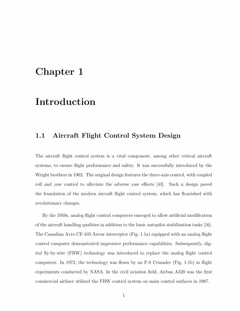
The Canadian Avro CF-105 Arrow interceptor (Fig. 1.1a) equipped with an analog flight
control computer demonstrated impressive performance capabilities. Subsequently, dig-
ital fly-by-wire (FBW) technology was introduced to replace the analog flight control
computers. In 1972, the technology was flown by an F-8 Crusader (Fig. 1.1b) in flight
experiments conducted by NASA. In the civil aviation field, Airbus A320 was the first
commercial airliner utilized the FBW control system on main control surfaces in 1987.
1
Chapter 1. Introduction 2
(a) Avro CF-105 Arrow (b) F-8 (c) Airbus A320
Fig. 1.1: Military and civil aircraft.Sources: (a) DND http://www.airforce.forces.gc.ca/v2/equip/resrc/images/hst/l-g/arrow4.jpg;
(b) NASA http://www.dfrc.nasa.gov/gallery/photo/F-8DFBW/Small/EC77-6988.jpg; (c) airliners.net
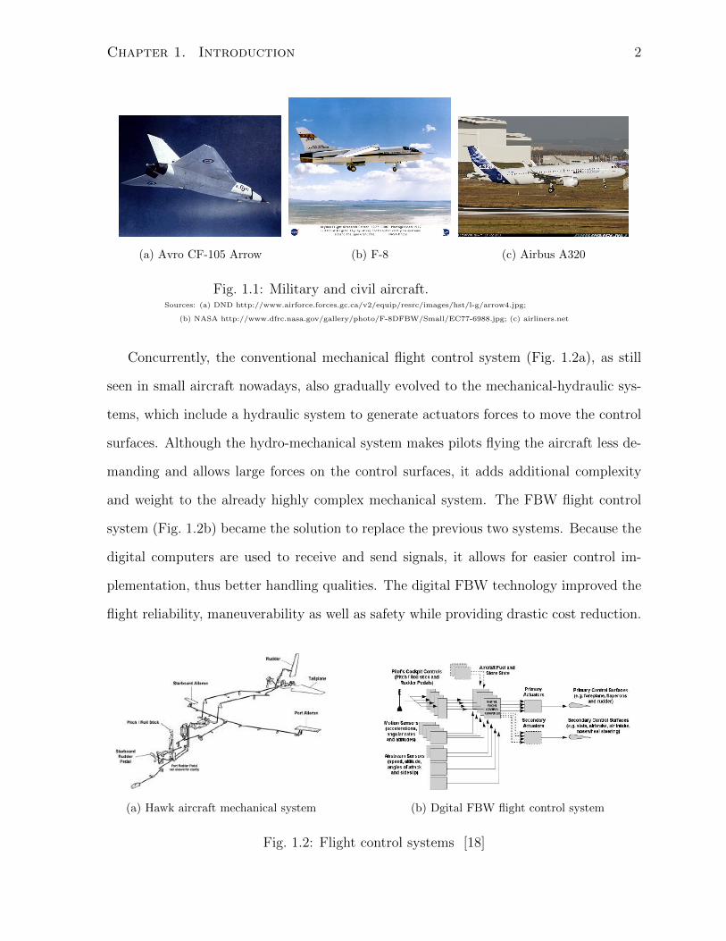
Concurrently, the conventional mechanical flight control system (Fig. 1.2a), as still
seen in small aircraft nowadays, also gradually evolved to the mechanical-hydraulic sys-
tems, which include a hydraulic system to generate actuators forces to move the control
surfaces. Although the hydro-mechanical system makes pilots flying the aircraft less de-
manding and allows large forces on the control surfaces, it adds additional complexity
and weight to the already highly complex mechanical system. The FBW flight control
system (Fig. 1.2b) became the solution to replace the previous two systems. Because the
digital computers are used to receive and send signals, it allows for easier control im-
plementation, thus better handling qualities. The digital FBW technology improved the
flight reliability, maneuverability as well as safety while providing drastic cost reduction.
(a) Hawk aircraft mechanical system (b) Dgital FBW flight control system
Fig. 1.2: Flight control systems [18]
Chapter 1. Introduction 3
1.2 Research Motivation
The advent of digital FBW system brings a new chapter to the flight control system
design. The computer-based system allows better handling, greater aircraft maneuver-
ability and agility, weight reduction and so on. These benefits come with the most
stringent safety requirement. For example, an FBW system must have the same level of
safety and integrity as the simple mechanical system. It means that the probability of
a failure occurring in the FBW system which would result in catastrophic consequences
to the aircraft must be less than 1 in 109 per flight hour [14]. The intense focus on the
safety level and the need to improve the system integrity require the FBW aircraft to
be fitted with a back up system. This system has the ability to generate fault-tolerant
control commands that take advantages of the system redundancy in terms of controls,
sensors, and computing. The control effector redundancy provides a unique opportunity
for the back up control system to reconfigure itself to mitigate and compensate for the
failure of the aircraft with the objective of increasing survivability.
In addition, recent civil aviation safety data show that about 16% of the accidents
that happened in between 1992 and 2007 belongs to the category of Loss of Control In-
flight (LOS-I), which is caused by pilot error, technical malfunctions, or unusual upsets
due to external disturbances [16]. For example, in the late 1970s an American Airlines
DC-10 crashed in Chicago (Flight 191, May 25, 1979) due to engine seperation. The pilot
only had 15s to react before the plane crashed. The subsequent investigations showed
the accident could have been avoided [36]. More recently, an El Al cargo Flight 1862
(October 4, 1992) fatal crash was also demonstated in simulation to be avoidable [31].
These catastrophic crashes underscore the need to have intelligent, fault-tolerant flight
control (FTFC) systems. NASA commenced the Integrated Resilient Aircraft Control
(IRAC) project of NASA Aviation Safety Program (AvSP) to investigate and research
advanced flight controls that can be implemented to ensure safety in the presence of
unforeseen, adverse conditions. Similarly, European GARTEUR Flight Mechanics Action
Chapter 1. Introduction 4
Group FM-AG(16) on fault-tolerant flight control has also focused on the topic.
In addition to the FBW system, the FTFC system is only activated when the fault is
positively detected and diagnosed on the aircraft. The FTFC system is specifically de-
signed to stabilize and control the aircraft without exacerbating the situation into a more
serious situation while ensuring post-damage performance with acceptable degradation
so that the survivability and safety are greatly enhanced.
1.3 Literature Review
The fault-tolerant flight control system design are reviewed in this section. In general,
fault-tolerant control systems can be categorized into passive and active systems. Passive
controllers are designed based on a pre-determined set of requirements. They are fixed
and are robust against a class of presumed faults [17]. Controllers need neither a fault
detection, isolation and diagnosis scheme nor controller reconfiguration, but only limited
fault-tolerant capabilities are achievable. On the other hand, as the name suggests, the
active controllers respond to the system malfunction by actively reconfiguring control laws
to ensure stability and performance requirements are met. Sometimes, certain degrees of
performance degradation have to be accepted due to severe damage. The overall design
objectives of fault-tolerant controllers are to meet the system transient and steady-state
performance requirements not only under normal operating conditions, but also in fault
situations. To achieve these objectives, a large number of controllers have been designed
and implemented on both linear and nonlinear systems. The rest of this section presents
some common control methods designed for fault-tolerant flight control, covering both
the passive and active systems.
Marcos and Balas [32] presented a quasi-linear parameter varying (LPV) model for
LPV control synthesis that guarantees stability and robustness of the closed loop sys-
tem. LPV was chosen to model the damaged aircraft because it is represented by its
varying parameter description. Three different linearization approaches were used in the
Chapter 1. Introduction 5
paper, namely Jacobian linearization, state transformation and function substitution.
Shin [49] presented an LPV model based on fault parameters. The fault parameters were
also scheduling parameters in this case and were estimated on-line by using a two-stage
adaptive Kalman filter. Aligned with the work of Shin, Shin and Gregory [48] presented
another LPV formulation that involved function substitution. Unlike the previous work,
aerodynamic coefficients were fitted from the plots and the uncertainties of which were
included in the model.
Maciejowski and Jones [31] applied Model Predictive Control (MPC) to the El Al
flight 1862 model based on the assumption that a perfect fault detection and isolation
model was available. Kale [26] and Miksch [35] also explored MPC as the control system.
However, the main disadvantage in their formulations [26,31,35] was that the cost func-
tion has two different horizons, predictive and control horizons. By doing so, however
the closed loop stability was not guaranteed and additional complexity is introduced. To
overcome the stability problem, Almeida and Leissling [2] presented a new formulation
using MPC in which fault-tolerant MPC with infinite prediction horizon approach was
studied. Since MPC is applied over a long horizon, it would be only possible to implement
such a method to dynamically slow systems, and hence not applicable to fault-tolerant
flight control systems. Very recently, Fabio [15] provided a possible alternative to solve
the problem by reducing the horizon to a shorter one.
The Sliding mode control (SMC) method was also studied extensively by [3, 4, 47].
In the first paper [3], Alwi et al made an assumption that there was no FDI available.
Unlike the MPC approach [31], the presented SMC did not require exact knowledge of
the post-damage aircraft. With the popularity of control allocation in the field of FTFC
systems, Shin et al [47] used the idea of control allocation, but an adaptive sliding mode
control method was implemented. Most of the research related to SMC are lack of a
detailed analysis in stability. As a result, in the paper by Alwi et al [4], the control
allocation and SMC were combined and a rigorous design procedure was presented.
Chapter 1. Introduction 6
Adaptive control is another popular method being widely used in the flight control
system [28, 40, 46]. A direct adaptive reconfigurable flight control method was proposed
by Kim et al [28] to deal with the nuisance of having a system identification process in the
indirect adaptive control. System identification was often used to accompany the indirect
adaptive control to handle the model mismatch and parameter uncertainty issues. The
timescale separation principle was applied in a model following scheme to control both
inner loop state and the outer loop state of the flight system simultaneously. Adaptive
control is often used in conjunction with a neural control scheme, particularly in nonlinear
dynamic systems. In the paper by Napolitano [40], an integrated sensor and actuator
failure detection, identification and accommodation within an FTFC system was studied.
Such an integration is able to detect failures and pass the information to the controller
with the goal of minimizing the false alarm rate and incorrect failure identification.
Lombaerts et al [30] presented the use of nonlinear dynamic inversion (NDI) technique
in which a real-time identified physical model of the damaged aircraft was included to
avoid NDIs sensitivity to modeling error. An Iterated Extended Kalman Filter (IEKF)
was used to estimate the aircraft states. The usage of which can potentially increase
the computational cost and lead to real-time implementation difficulties. DI and MPC
were combined together as a control method in [25] to tackle the FTFC problem. The
combination is intuitive since the DI provides a linearized model that MPC can work on.
As a result, a reconfigurable, nonlinear controller was designed.
The above literature review covers some of the prominent control methods used in
the field of fault-tolerant flight control system. However, few of the existing methods
provide a systematic and efficient design approach to deal with the problem. Necessary
features such as the flexibility and versatility, which these control methods lack, make the
design process difficult, especially when transferring from one model to another one. It is
also important to recognize the inherent nonlinear nature of aircraft dynamics. Nonlinear
control methods may be better to handle the fault-tolerant tasks. As a result, a nonlinear
Chapter 1. Introduction 7
control method that possesses the systematic and efficient design approach is proposed
in this research to deal with damaged aircraft.
Fault-tolerant flight control systems are often complemented by a robust guidance
system to achieve safe landing objective. For example, Menon et al. [33] implemented a
robust guidance algorithm for impaired aircraft based on a point mass nonlinear aircraft
model. The guidance algorithm was formulated with the finite interval differential game.
The guidance commands then were inverse transformed into the roll, pitch and yaw
attitude commands. Chawla et al [6] studied a partial integrated guidance and control
system based on the nonlinear dynamic inversion to perform obstacle avoidance of UAVs.
The collision cone concept was used in the derivation to transform the problem into a
sequential target interception problem. The guidance algorithm was then derived under
the frame of a collision cone. Other guidance algorithms based on optimization methods,
such as mixed integer linear programming or model predictive control techniques are not
suitable in our applications due to their heavy requirement of computational resources.
In this thesis, a robust, feedback based guidance algorithm is implemented for dam-
aged aircraft. The guidance algorithm takes into consideration damaged aircraft dynam-
ics to adjust its commands in a feedback fashion. It also needs little modification to
the existing control system architectures, unlike the above mentioned ones which require
guidance command transformations.
1.4 Research Objectives & Contribution
This research focuses on the design of nonlinear fault-tolerant flight control laws to en-
sure flight safety in the presence of adverse conditions. Additionally, it investigates the
integration of guidance laws and control laws in the context of damaged aircraft to guar-
antee fast response, and safe landing. The benefits of the proposed framework over the
existing ones are also explored.
Although there have been many control laws designed for the purpose of mitigat-
Chapter 1. Introduction 8
ing faults and recovering the flight performance, few have demonstrated the ability to
integrate with guidance laws to ensure safe landing. In addition, most of the exiting
controllers, as mentioned in the previous section, are categorized as linear controllers,
which require extensive gain scheduling to cover a wide flight envelope. This work aims
to provide a sophisticated, yet designer-friendly solution to achieve the objective of safe
landing of the damaged aircraft while taking the advantage of nonlinear control.
The benefits of integration are critical in the damaged case. The smooth integration
can support the post-damage planning, guidance, and control in a unified manner, which
not only saves precious time, but also increases the survivability and safety.
This work contributes to the research and development of the fault-tolerant flight
control system mainly in the following areas:
• To develop a nonlinear fault-tolerant flight control system to handle damaged air-
craft;
• To implement the guidance and control laws to expedite post-damage recovery and
ensure safe landing;
• To investigate and verify the proposed framework performance by comparing with
the existing control method.
1.5 Thesis Organization
The thesis is organized in the following manner. Chapter 2 presents both healthy and
damaged aircraft dynamics and modeling. The fault-tolerant flight guidance and control
problem is introduced in Chapter 3, which covers the problem formulation and design
framework. Chapter 4 focuses on the aircraft guidance law design. In Chapter 5, non-
linear fault-tolerant control methods are discussed. A novel nonlinear adaptive control
law is derived in Chapter 6. Simulation studies are performed in that chapter to demon-
strate its promising results. Finally, the concluding remarks and possible future works
are offered in Chapter 7.
Chapter 2
Aircraft Dynamics
This chapter presents the aircraft dynamics. In Section 2.2, the general nonlinear equa-
tions of motion (EOM) are derived and formulated. Section 2.3 introduces the nonlinear
aerodynamic coefficients that are included in the models. Section 2.4 deals with the
damaged aircraft modeling and Section 2.5 presents the optimization based trim routine
used to seek the steady state level flight condition.
2.1 Introduction
In this chapter, the general six degrees of freedom (6DoF) nonlinear EOM are introduced.
Two aircraft models, Boeing 747-100/200 and NASA Generic Transport Model (GTM),
are used throughout the thesis as simulation test beds. Both models are covered in details
in Section 2.3. The Damaged aircraft modeling is studied in Section 2.4. Several damage
scenarios as well as their possible outcomes are reviewed in that section.
2.2 Aircraft Modeling
Before diving into the derivation of the equations of motion, it is important to establish
the frames of reference. Throughout the thesis, the following right-handed and orthogonal
reference frames are used: the earth-fixed inertial reference frame, FE; the vehicle carried
local earth reference frame, FO whose origin is fixed at the centre of gravity of the vehicle
9
Chapter 2. Aircraft Dynamics 10
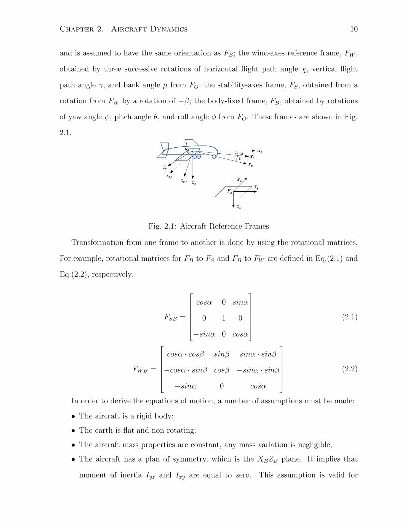
and is assumed to have the same orientation as FE; the wind-axes reference frame, FW ,
obtained by three successive rotations of horizontal flight path angle χ, vertical flight
path angle γ, and bank angle µ from FO; the stability-axes frame, FS, obtained from a
rotation from FW by a rotation of −β; the body-fixed frame, FB, obtained by rotations
of yaw angle ψ, pitch angle θ, and roll angle φ from FO. These frames are shown in Fig.
2.1.
Fig. 2.1: Aircraft Reference Frames
Transformation from one frame to another is done by using the rotational matrices.
For example, rotational matrices for FB to FS and FB to FW are defined in Eq.(2.1) and
Eq.(2.2), respectively.
FSB =
cosα 0 sinα
0 1 0
−sinα 0 cosα
(2.1)
FWB =
cosα · cosβ sinβ sinα · sinβ
−cosα · sinβ cosβ −sinα · sinβ
−sinα 0 cosα
(2.2)
In order to derive the equations of motion, a number of assumptions must be made:
• The aircraft is a rigid body;
• The earth is flat and non-rotating;
• The aircraft mass properties are constant, any mass variation is negligible;
• The aircraft has a plan of symmetry, which is the XBZB plane. It implies that
moment of inertia Iyz and Ixy are equal to zero. This assumption is valid for
Chapter 2. Aircraft Dynamics 11
undamaged aircraft. When aircraft suffer from asymmetric damage, the assumption
does not apply any more;
2.2.1 Nonlinear Equations of Motion
The aircraft equations of motion can be derived from Newton’s Second Law. Mathemat-
ically, Newton’s Second Law can be expressed as the following in the inertial frame
F =d
dt(mVt)|E (2.3)
M =d
dt(H)|E (2.4)
where F is the sum of all external forces; m is the aircraft mass; M represents the sum of
all external moments about the centre of the mass; H is the angular momentum about
the centre of mass.
The above equations can be written in the body-fixed frame, FB as
F =d
dt(mVt)|B + ω ×mVt (2.5)
M =d
dt(H)|B + ω ×H (2.6)
where ω is the total angular velocity of the aircraft with respect to the Earth. The vector
terms in Eq.(2.5) and Eq.(2.6) can be expressed as
Vt = ui + vj + wk (2.7)
ω = pi + qj + rk (2.8)
H = Iω (2.9)
where I is defined as
I =
Ix 0 −Ixz
0 Iy 0
−Ixz 0 Iz
(2.10)
Chapter 2. Aircraft Dynamics 12
Substituting Eq.(2.7)-Eq.(2.9) into Eq.(2.5) and Eq.(2.6) and expanding terms yields,
Fx = m(u+ qw − rv) (2.11)
Fy = m(v + ru− pw) (2.12)
Fz = m(w + pv − qu) (2.13)
Mx = pIx − rIxz + qr(Iz − Iy)− pqIxz (2.14)
My = qIy + pq(Ix − Iz) + (p2 − r2)Ixz (2.15)
Mz = rIz − pIxz + pq(Iy − Ix) + qrIxz (2.16)
where the external forces are the aerodynamic forces, thrust forces and gravity forces and
the external moments include the aerodynamic moments and the engine moments.
Fx = qSCxb + FTx −mgsinθ (2.17)
Fy = qSCyb + FTy +mgcosθsinφ (2.18)
Fz = qSCzb + FTz +mgcosθcosφ (2.19)
Mx = qSbClb +Mengx (2.20)
My = qScCmb +Mengy (2.21)
Mz = qSbCnb +Mengz (2.22)
where q = 12ρV 2
t is the dynamic pressure. The equations presented above are collected
together and rearranged into a set of twelve first order, aircraft equations of motion.
Force equations:
u = rv − qw −mgsinθ +1
m(qSCxb + FTx) (2.23)
v = −ru+ pw + gsinφcosθ +1
m(qSCyb + FTy) (2.24)
w = qu− pv + gcosφcosθ +1
m(qSCyb + FTy) (2.25)
Chapter 2. Aircraft Dynamics 13
Kinematic equations:φ
θ
ψ
=
1 sinφ · tanθ cosφ · tanθ
0 cosφ −sinφ
0 sinφcosθ
cosφcosθ
p
q
r
(2.26)
Moment equations:p
q
r
=
Ixx 0 −Ixz
0 Iyy 0
−Ixz 0 Izz
−1
Mx + (Iyy − Izz)qr + Ixzpq
My + (Izz − Ixx)pr + Ixz(r2 − p2)
Mz + (Ixx − Iyy)pq − Ixzqr
(2.27)
Navigation equations:xe
ye
he
=
cosθ · cosψ sinφ · sinθ · cosψ − cosφ · sinψ cosφ · sinθ · cosψ + sinφ · sinψ
cosθ · sinψ sinφ · sinθ · sinψ + cosφ · cosψ cosφ · sinθ · sinψ − sinφ · cosψ
sinθ −sinφ · cosθ −cosφ · cosθ
u
v
w
(2.28)
where (u, v, w) are the velocity components; (φ, θ, ψ) are the Euler angles, roll, pitch and
yaw angle; (p, q, r) are the roll, pitch and yaw rate; (xe, ye, he) are the inertial positions.
For the fault-tolerant flight control design, it is more sensible to introduce the air-
speed, angle of attack and slideslip angle as state variables to replace u, v, w in the force
equations. The main reasons are: first of all, Some of aerodynamic derivatives obtained
from wind tunnel or flight tests, are tabulated based on α, β. As a result, it is easier
to use these variables as state instead of converting from other variables. Thus, greater
accuracy may be preserved. Secondly, when aircraft suffer from abnormalities in flight,
their behavior can be difficult to predict. For instance, the upper limit of the pitch rate
q may reach as high as 0.2rad/s, similar to the case of agile aircraft and aircraft can fly
at a high airspeed (e.g. Vt = 60m/s). It means the term qu in eq.(2.25) may become as
large as 12g’s. However, in reality the upper limit of the normal acceleration can be only
a few g’s. Hence greater accelerations are introduced into equations because of the high
rotation rates which the body-axes experience. This means much less favorable computer
Chapter 2. Aircraft Dynamics 14
scaling and hence much poorer solution accuracy for a given computer precision if the
simulation is based on u, v and w instead of Vt, α, and β [45]. The following equations are
used to replace the force equations. Their derivations are included in the Appendix A.
α =1
mVtcosβ(−Fxsinα + Fzcosα +mVt(−pcosαsinβ + qcosβ − rsinαsinβ)) (2.29)
β =1
mVt(−Fxcosαsinβ + Fycosβ − Fzsinαsinβ −mVt(−psinα + rcosα)) (2.30)
Vt =1
m(Fxcosαcosβ + Fysinβ + Fzcosβsinα) (2.31)
Thus, the 6DOF state vector is
x =
[Vt α β φ θ ψ p q r xe ye he
]T(2.32)
2.3 Nonlinear Aerodynamic Coefficients
2.3.1 Boeing 747-100/200
As mentioned earlier, both B747 and GTM models are considered in the thesis. In this
section, the B747 nonlinear aerodynamic coefficients are presented. The NASA GTM
ones are briefly reviewed later in this section.
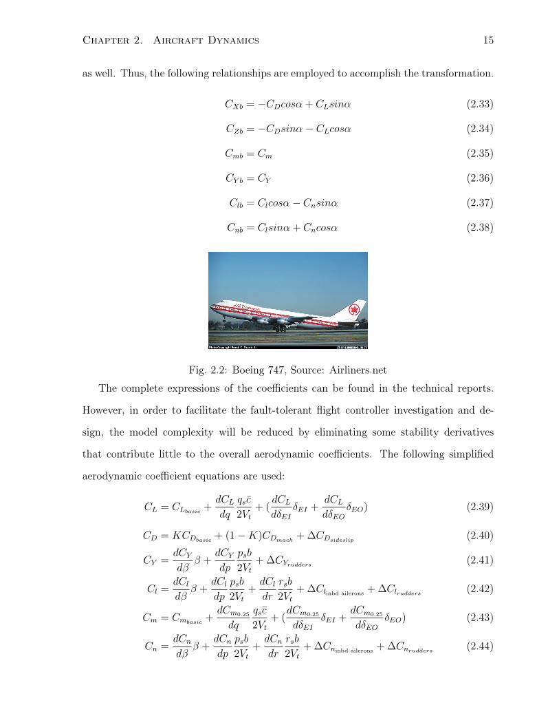
The Boeing 747-100/200 (Fig. 2.2) is an inter-continental wide-body transport with
four turbofan jet engines designed to operate from international airports. It exhibits a
wide array of characteristics (leading and trailing edge flaps, spoilers, variety of control
surfaces, four fan jet engines...) which make it the perfect representative for any of the
commercial airplanes flying today. The physical properties and aerodynamic data used
in this thesis are obtained from NASA technical reports [22,23]. The aerodynamic coef-
ficients are based on a number of stability derivatives, which are defined in the stability
frame of reference. Since the EOM are in FB, the aerodynamic coefficients must be in FB
Chapter 2. Aircraft Dynamics 15
as well. Thus, the following relationships are employed to accomplish the transformation.
CXb = −CDcosα + CLsinα (2.33)
CZb = −CDsinα− CLcosα (2.34)
Cmb = Cm (2.35)
CY b = CY (2.36)
Clb = Clcosα− Cnsinα (2.37)
Cnb = Clsinα + Cncosα (2.38)
Fig. 2.2: Boeing 747, Source: Airliners.net
The complete expressions of the coefficients can be found in the technical reports.
However, in order to facilitate the fault-tolerant flight controller investigation and de-
sign, the model complexity will be reduced by eliminating some stability derivatives
that contribute little to the overall aerodynamic coefficients. The following simplified
aerodynamic coefficient equations are used:
CL = CLbasic +dCLdq
qsc
2Vt+ (
dCLdδEI
δEI +dCLdδEO
δEO) (2.39)
CD = KCDbasic + (1−K)CDmach + ∆CDsideslip (2.40)
CY =dCYdβ
β +dCYdp
psb
2Vt+ ∆CYrudders (2.41)
Cl =dCldβ
β +dCldp
psb
2Vt+dCldr
rsb
2Vt+ ∆Clinbd ailerons
+ ∆Clrudders (2.42)
Cm = Cmbasic +dCm0.25
dq
qsc
2Vt+ (
dCm0.25
dδEIδEI +
dCm0.25
dδEOδEO) (2.43)
Cn =dCndβ
β +dCndp
psb
2Vt+dCndr
rsb
2Vt+ ∆Cninbd ailerons
+ ∆Cnrudders (2.44)
Chapter 2. Aircraft Dynamics 16
In the cases of lift and pitching moment coefficients, the contributing factors include
the basic lift and pitching moment coefficients, the dynamic stability derivatives dCLdq
and dCmdq
as well as the contributions from the both inboard and outboard elevators,
respectively. It is also assumed in this case that the centre of gravity coincides with the
aerodynamic centre at the quarter chord location. The drag coefficient, CD, is mainly
dictated by the basic drag coefficient, drag coefficient due to Mach number as well as the
sideslip angle. K is an aircraft specific constant. CY is determined from the contribution
of β, p, and rudders. Similarly, Cl and Cn depend on β, p, r, inboard ailerons, and
rudders.
The stability derivatives in Eq.(2.39)- Eq.(2.44) are then put into the look-up tables
(LUT) in Matlab for easy access during the simulation. Thus, the nonlinear B747 model
is obtained using the reduced aerodynamic coefficients and the previous derived nonlinear
EOM.
2.3.2 NASA GTM
The NASA GTM model is provided in a Simulink package (Fig. 2.3). It includes the
comprehensive aircraft information in terms of aerodynamic look-up tables as well as
Simulink blocks. The difference between the previous mentioned EOM and the one
implemented in the GTM model is that the aerodynamic forces are calculated based on
the center of pressure (CP) instead of the aerodynamic center (ac). It is believed that
because of the extensive wind tunnel data, such practices becomes possible. As a result,
the moment equation requires modification to accommodate the change. In addition, the
CG location is no longer assumed at the ac as in the case of B747. The moment equation
implemented in the model is the following:
M = Maero + Meng + (CP−CG)× Faero (2.45)
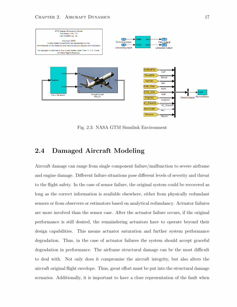
Chapter 2. Aircraft Dynamics 17
Fig. 2.3: NASA GTM Simulink Environment
2.4 Damaged Aircraft Modeling
Aircraft damage can range from single component failure/malfunction to severe airframe
and engine damage. Different failure situations pose different levels of severity and threat
to the flight safety. In the case of sensor failure, the original system could be recovered as
long as the correct information is available elsewhere, either from physically redundant
sensors or from observers or estimators based on analytical redundancy. Actuator failures
are more involved than the sensor case. After the actuator failure occurs, if the original
performance is still desired, the remaindering actuators have to operate beyond their
design capabilities. This means actuator saturation and further system performance
degradation. Thus, in the case of actuator failures the system should accept graceful
degradation in performance. The airframe structural damage can be the most difficult
to deal with. Not only does it compromise the aircraft integrity, but also alters the
aircraft original flight envelope. Thus, great effort must be put into the structural damage
scenarios. Additionally, it is important to have a close representation of the fault when
Chapter 2. Aircraft Dynamics 18
designing the fault-tolerant control. Table 2.1 lists a number of common fault scenarios
and their respective effects.
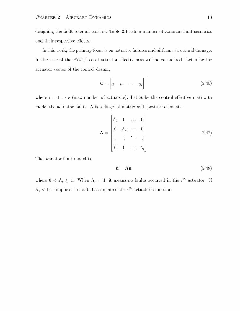
In this work, the primary focus is on actuator failures and airframe structural damage.
In the case of the B747, loss of actuator effectiveness will be considered. Let u be the
actuator vector of the control design,
u =
[u1 u2 · · · ui
]T(2.46)
where i = 1 · · · s (max number of actuators). Let Λ be the control effective matrix to
model the actuator faults. Λ is a diagonal matrix with positive elements.
Λ =
Λ1 0 . . . 0
0 Λ2 . . . 0
......
. . ....
0 0 . . . Λi
(2.47)
The actuator fault model is
u = Λu (2.48)
where 0 < Λi ≤ 1. When Λi = 1, it means no faults occurred in the ith actuator. If
Λi < 1, it implies the faults has impaired the ith actuator’s function.
Chapter 2. Aircraft Dynamics 19
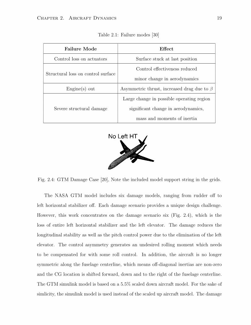
Table 2.1: Failure modes [30]
Failure Mode Effect
Control loss on actuators Surface stuck at last position
Structural loss on control surfaceControl effectiveness reduced
minor change in aerodynamics
Engine(s) out Asymmetric thrust, increased drag due to β
Severe structural damage
Large change in possible operating region
significant change in aerodynamics,
mass and moments of inertia
Fig. 2.4: GTM Damage Case [20], Note the included model support string in the grids.
The NASA GTM model includes six damage models, ranging from rudder off to
left horizontal stabilizer off. Each damage scenario provides a unique design challenge.
However, this work concentrates on the damage scenario six (Fig. 2.4), which is the
loss of entire left horizontal stabilizer and the left elevator. The damage reduces the
longitudinal stability as well as the pitch control power due to the elimination of the left
elevator. The control asymmetry generates an undesired rolling moment which needs
to be compensated for with some roll control. In addition, the aircraft is no longer
symmetric along the fuselage centerline, which means off-diagonal inertias are non-zero
and the CG location is shifted forward, down and to the right of the fuselage centerline.
The GTM simulink model is based on a 5.5% scaled down aircraft model. For the sake of
simlicity, the simulink model is used instead of the scaled up aircraft model. The damage
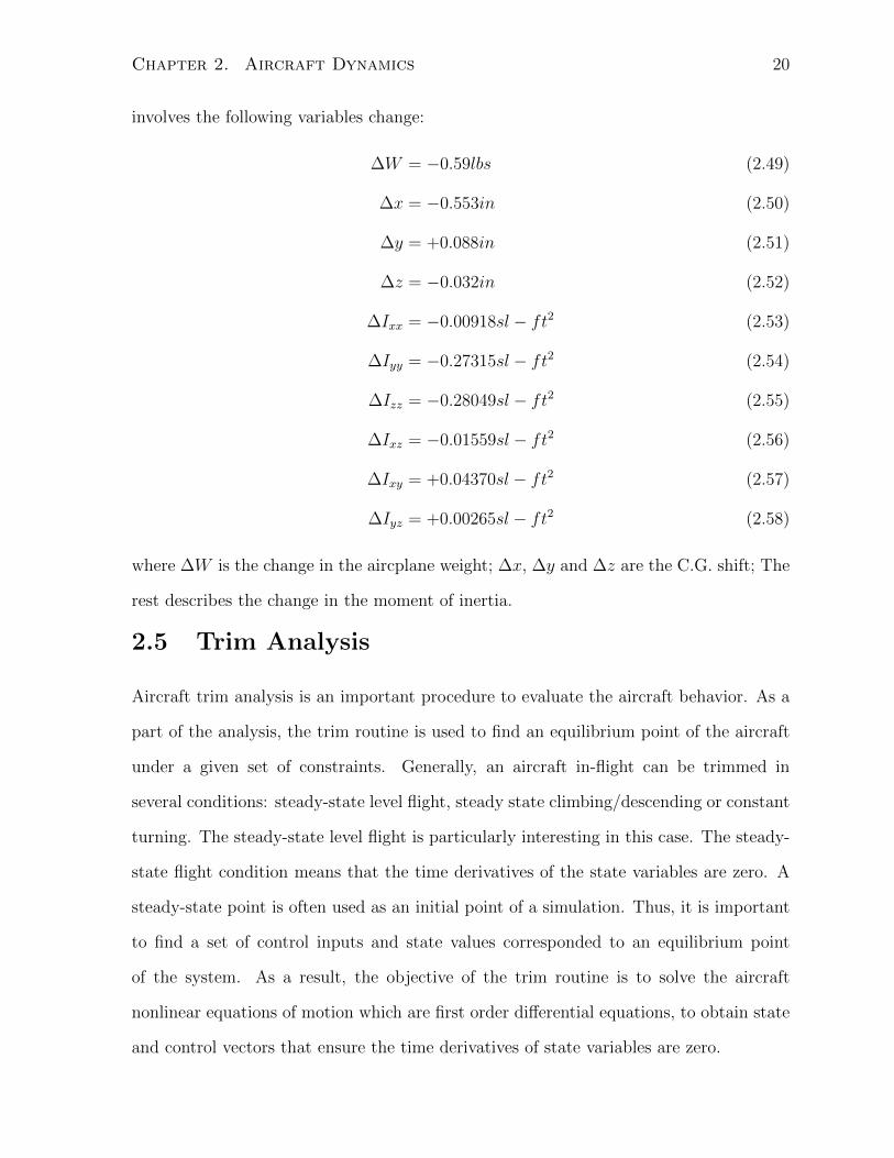
Chapter 2. Aircraft Dynamics 20
involves the following variables change:
∆W = −0.59lbs (2.49)
∆x = −0.553in (2.50)
∆y = +0.088in (2.51)
∆z = −0.032in (2.52)
∆Ixx = −0.00918sl − ft2 (2.53)
∆Iyy = −0.27315sl − ft2 (2.54)
∆Izz = −0.28049sl − ft2 (2.55)
∆Ixz = −0.01559sl − ft2 (2.56)
∆Ixy = +0.04370sl − ft2 (2.57)
∆Iyz = +0.00265sl − ft2 (2.58)
where ∆W is the change in the aircplane weight; ∆x, ∆y and ∆z are the C.G. shift; The
rest describes the change in the moment of inertia.
2.5 Trim Analysis
Aircraft trim analysis is an important procedure to evaluate the aircraft behavior. As a
part of the analysis, the trim routine is used to find an equilibrium point of the aircraft
under a given set of constraints. Generally, an aircraft in-flight can be trimmed in
several conditions: steady-state level flight, steady state climbing/descending or constant
turning. The steady-state level flight is particularly interesting in this case. The steady-
state flight condition means that the time derivatives of the state variables are zero. A
steady-state point is often used as an initial point of a simulation. Thus, it is important
to find a set of control inputs and state values corresponded to an equilibrium point
of the system. As a result, the objective of the trim routine is to solve the aircraft
nonlinear equations of motion which are first order differential equations, to obtain state
and control vectors that ensure the time derivatives of state variables are zero.
Chapter 2. Aircraft Dynamics 21
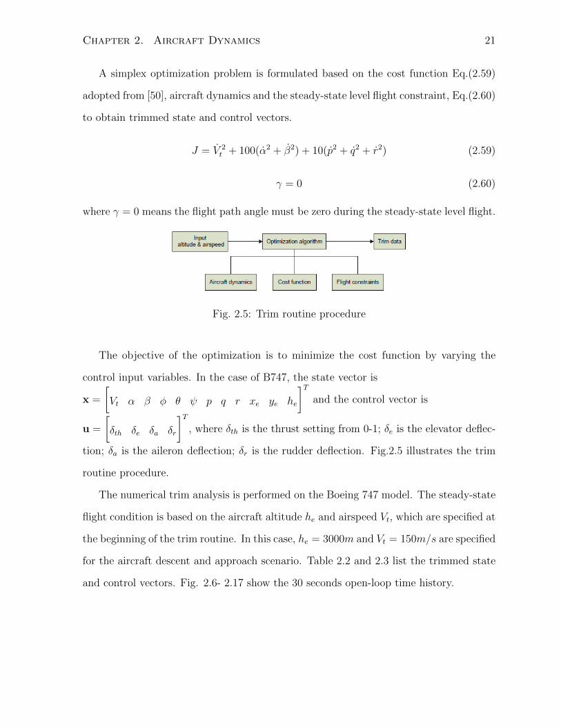
A simplex optimization problem is formulated based on the cost function Eq.(2.59)
adopted from [50], aircraft dynamics and the steady-state level flight constraint, Eq.(2.60)
to obtain trimmed state and control vectors.
J = V 2t + 100(α2 + β2) + 10(p2 + q2 + r2) (2.59)
γ = 0 (2.60)
where γ = 0 means the flight path angle must be zero during the steady-state level flight.
Fig. 2.5: Trim routine procedure
The objective of the optimization is to minimize the cost function by varying the
control input variables. In the case of B747, the state vector is
x =
[Vt α β φ θ ψ p q r xe ye he
]Tand the control vector is
u =
[δth δe δa δr
]T, where δth is the thrust setting from 0-1; δe is the elevator deflec-
tion; δa is the aileron deflection; δr is the rudder deflection. Fig.2.5 illustrates the trim
routine procedure.
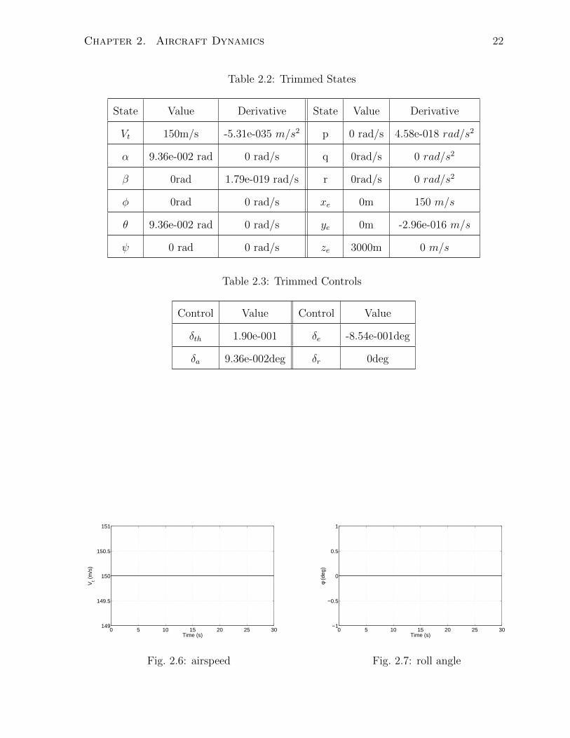
The numerical trim analysis is performed on the Boeing 747 model. The steady-state
flight condition is based on the aircraft altitude he and airspeed Vt, which are specified at
the beginning of the trim routine. In this case, he = 3000m and Vt = 150m/s are specified
for the aircraft descent and approach scenario. Table 2.2 and 2.3 list the trimmed state
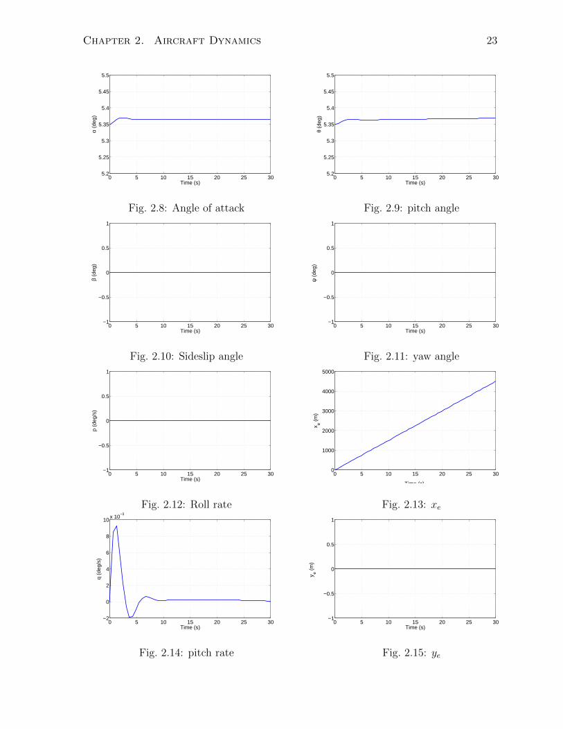
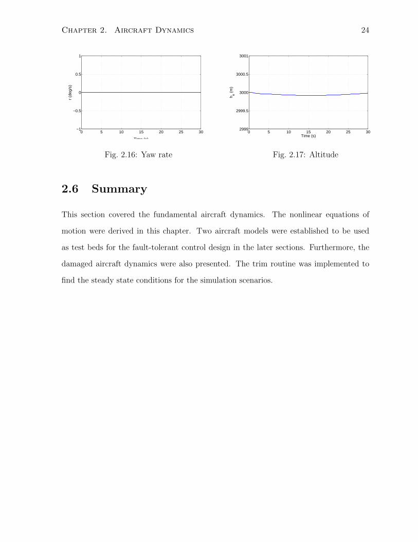
and control vectors. Fig. 2.6- 2.17 show the 30 seconds open-loop time history.
Chapter 2. Aircraft Dynamics 22
Table 2.2: Trimmed States
State Value Derivative State Value Derivative
Vt 150m/s -5.31e-035 m/s2 p 0 rad/s 4.58e-018 rad/s2
α 9.36e-002 rad 0 rad/s q 0rad/s 0 rad/s2
β 0rad 1.79e-019 rad/s r 0rad/s 0 rad/s2
φ 0rad 0 rad/s xe 0m 150 m/s
θ 9.36e-002 rad 0 rad/s ye 0m -2.96e-016 m/s
ψ 0 rad 0 rad/s ze 3000m 0 m/s
Table 2.3: Trimmed Controls
Control Value Control Value
δth 1.90e-001 δe -8.54e-001deg
δa 9.36e-002deg δr 0deg
0 5 10 15 20 25 30149
149.5
150
150.5
151
Time (s)
Vt (
m/s
)
Fig. 2.6: airspeed
0 5 10 15 20 25 30−1
−0.5
0
0.5
1
Time (s)
φ (d
eg)
Fig. 2.7: roll angle
Chapter 2. Aircraft Dynamics 23
0 5 10 15 20 25 305.2
5.25
5.3
5.35
5.4
5.45
5.5
Time (s)
α (d
eg)
Fig. 2.8: Angle of attack
0 5 10 15 20 25 305.2
5.25
5.3
5.35
5.4
5.45
5.5
Time (s)
θ (d
eg)
Fig. 2.9: pitch angle
0 5 10 15 20 25 30−1
−0.5
0
0.5
1
Time (s)
β (d
eg)
Fig. 2.10: Sideslip angle
0 5 10 15 20 25 30−1
−0.5
0
0.5
1
Time (s)
ψ (
deg)
Fig. 2.11: yaw angle
0 5 10 15 20 25 30−1
−0.5
0
0.5
1
Time (s)
p (d
eg/s
)
Fig. 2.12: Roll rate
0 5 10 15 20 25 300
1000
2000
3000
4000
5000
Time (s)
x e (m
)
Fig. 2.13: xe
0 5 10 15 20 25 30−2
0
2
4
6
8
10x 10
−3
Time (s)
q (d
eg/s
)
Fig. 2.14: pitch rate
0 5 10 15 20 25 30−1
−0.5
0
0.5
1
Time (s)
y e (m
)
Fig. 2.15: ye
Chapter 2. Aircraft Dynamics 24
0 5 10 15 20 25 30−1
−0.5
0
0.5
1
Time (s)
r (d
eg/s
)
Fig. 2.16: Yaw rate
0 5 10 15 20 25 302999
2999.5
3000
3000.5
3001
Time (s)
h e (m
)
Fig. 2.17: Altitude
2.6 Summary
This section covered the fundamental aircraft dynamics. The nonlinear equations of
motion were derived in this chapter. Two aircraft models were established to be used
as test beds for the fault-tolerant control design in the later sections. Furthermore, the
damaged aircraft dynamics were also presented. The trim routine was implemented to
find the steady state conditions for the simulation scenarios.
Chapter 3
Fault-tolerant Flight Guidance and
Control Problem
3.1 Introduction
In this chapter, the fault-tolerant flight guidance and control problem is identified and
formulated and the guidance law design is derived. The objective is to provide a feasible
framework that is capable of handling aircraft that have suffered from damage so that
stabilization and safe landing are achieved. The framework comprises the guidance and
control loops. Each loop has its own design approach and objective, but overall acts in
an integrated, continuous fashion.
3.2 Problem Formulation
In this section, a detailed description of the fault-tolerant flight guidance and control
problem is introduced. The proposed framework that provides a feasible and viable
solution is also presented in the section. When the aircraft encounters damage in flight,
the conventional control design may not be adequate and robust enough to handle the
situation. Eventually, the aircraft may become uncontrollable and unstable. Most of the
time, human pilot intervention is required to prevent the situation from deteriorating to
25
Chapter 3. Fault-tolerant Flight Guidance and Control Problem 26
the worst. However, human error is becoming a major contributing factor to aviation
accidents. Thus, it is desired to implement the advanced control system that is capable
of actively providing intelligent and effective actuator control in such situations as well
as to backup the conventional flight control in normal flight conditions.
In addition, damaged aircraft can behave drastically different from the original aircraft
specifications. The flight envelope can be altered as well. Since the aircraft dynamics
are intrinsically nonlinear, linear control methods sometimes are not adequate to handle
the complex dynamics. The nonlinear robust controller on the other hand is able to
tolerant significant aircraft parameter variation. For sudden, large scale behavior changes,
nonlinear controller is far superior than the linear controller which may not be able to
control the plant at all. The nonlinear controller does not require extensive and time-
consuming gain scheduling due to the large number of design points. The unpredictable
nature of damaged scenarios can also increase the level of complexity of gain scheduling in
the linear controller. Thus, the nonlinear controller is more suitable in the fault-tolerant
flight control.
Furthermore, the ultimate goal for any damaged aircraft is to land safely. A robust
guidance law is a pre-requisite for the control system. The robust guidance law should
take the altered aerodynamics and performance change into consideration when gener-
ating guidance commands. In addition, from a practical point of view, it is beneficial to
have the robust guidance design fitted into the existing flight control design system so
that little system modification is necessary.
The proposed fault-tolerant flight guidance and control framework addresses the issues
mentioned above and provides a sophisticated system to deal with damaged aircraft.
Fig. 3.1 depicts the proposed system.
The control part of the system adopts the conventional three loop flight control system
design with a separate speed controller. Alternatively, an integrated speed controller
can be augmented with the inner loop. Since the guidance loop generates the airspeed
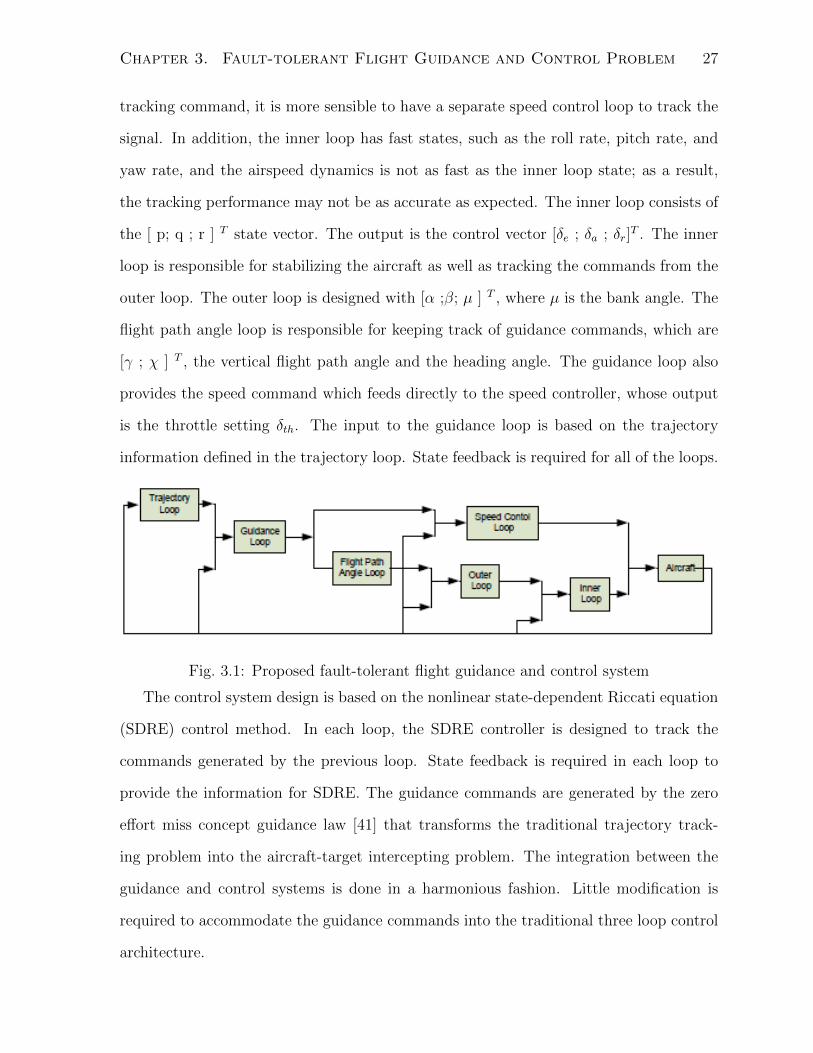
Chapter 3. Fault-tolerant Flight Guidance and Control Problem 27
tracking command, it is more sensible to have a separate speed control loop to track the
signal. In addition, the inner loop has fast states, such as the roll rate, pitch rate, and
yaw rate, and the airspeed dynamics is not as fast as the inner loop state; as a result,
the tracking performance may not be as accurate as expected. The inner loop consists of
the [ p; q ; r ] T state vector. The output is the control vector [δe ; δa ; δr]T . The inner
loop is responsible for stabilizing the aircraft as well as tracking the commands from the
outer loop. The outer loop is designed with [α ;β; µ ] T , where µ is the bank angle. The
flight path angle loop is responsible for keeping track of guidance commands, which are
[γ ; χ ] T , the vertical flight path angle and the heading angle. The guidance loop also
provides the speed command which feeds directly to the speed controller, whose output
is the throttle setting δth. The input to the guidance loop is based on the trajectory
information defined in the trajectory loop. State feedback is required for all of the loops.
Fig. 3.1: Proposed fault-tolerant flight guidance and control system
The control system design is based on the nonlinear state-dependent Riccati equation
(SDRE) control method. In each loop, the SDRE controller is designed to track the
commands generated by the previous loop. State feedback is required in each loop to
provide the information for SDRE. The guidance commands are generated by the zero
effort miss concept guidance law [41] that transforms the traditional trajectory track-
ing problem into the aircraft-target intercepting problem. The integration between the
guidance and control systems is done in a harmonious fashion. Little modification is
required to accommodate the guidance commands into the traditional three loop control
architecture.
Chapter 3. Fault-tolerant Flight Guidance and Control Problem 28
3.3 Remarks
The proposed fault-tolerant flight guidance and control framework is the backbone of the
work. Not only does it provide the guideline to the guidance and control systems design,
but also illustrates a sophisticated and advanced system. In the following chapters, the
actual system design work are carried out in details. The flight simulation results are
also included.
3.4 Aircraft Guidance Law Design
In this section, the aircraft guidance law design is presented. The guidance law is used in
the framework to provide the flight path angle, the heading angle as well as the airspeed
commands. Additionally, the guidance law can be readily fit into the existing control
system architecture so that little modification is required during the system integration.
In the following sections, the detailed design is based on the work of No et al. [41].
The guidance system is based on the concept of zero effort miss, which is a common
notion in the missile guidance community and has been used in a number of proportional
navigation guidance laws [56]. Essentially, the aircraft under the guidance law commands
tries to intercept the reference trajectory on which an ideal imaginary aircraft flies. The
guidance law navigates the aircraft to follow the imaginary aircraft as close as possible.
By doing so, the trajectory tracking objective is achieved with minimum error. Thus, the
traditional trajectory tracking problem is reformulated into an aircraft-target intercept
problem.
3.5 Guidance Law Design
The core of the guidance law is the zero effort miss concept. Since the guidance law is
based on the aircraft-target interception problem, the zero effort vector is defined in such
a scenario. Let there be an ideal, imaginary target aircraft flying on the trajectory. The
Chapter 3. Fault-tolerant Flight Guidance and Control Problem 29
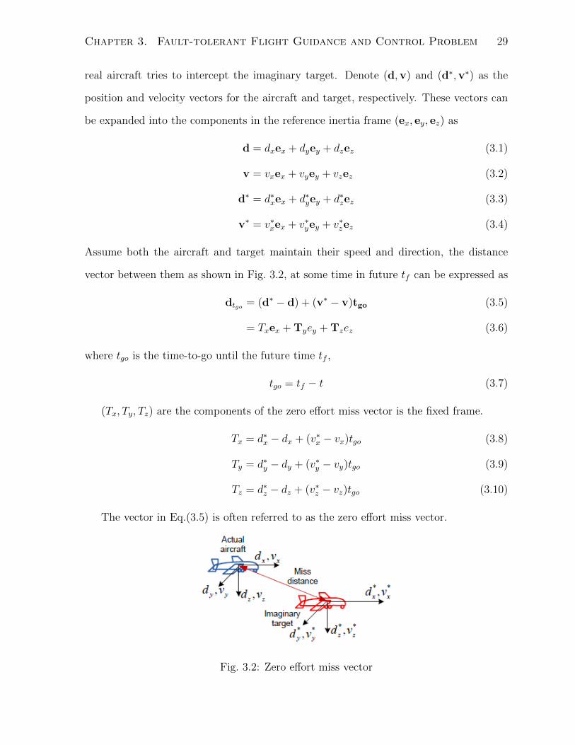
real aircraft tries to intercept the imaginary target. Denote (d,v) and (d∗,v∗) as the
position and velocity vectors for the aircraft and target, respectively. These vectors can
be expanded into the components in the reference inertia frame (ex, ey, ez) as
d = dxex + dyey + dzez (3.1)
v = vxex + vyey + vzez (3.2)
d∗ = d∗xex + d∗yey + d∗zez (3.3)
v∗ = v∗xex + v∗yey + v∗zez (3.4)
Assume both the aircraft and target maintain their speed and direction, the distance
vector between them as shown in Fig. 3.2, at some time in future tf can be expressed as
dtgo = (d∗ − d) + (v∗ − v)tgo (3.5)
= Txex + Tyey + Tzez (3.6)
where tgo is the time-to-go until the future time tf ,
tgo = tf − t (3.7)
(Tx, Ty, Tz) are the components of the zero effort miss vector is the fixed frame.
Tx = d∗x − dx + (v∗x − vx)tgo (3.8)
Ty = d∗y − dy + (v∗y − vy)tgo (3.9)
Tz = d∗z − dz + (v∗z − vz)tgo (3.10)
The vector in Eq.(3.5) is often referred to as the zero effort miss vector.
Fig. 3.2: Zero effort miss vector
Chapter 3. Fault-tolerant Flight Guidance and Control Problem 30
The actual guidance commands are derived through the use of a Lyapunov-like func-
tion.
V =1
2dtgo · dtgo (3.11)
=1
2(T 2
x + T 2y + T 2
z ) (3.12)
Taking time derivative of Eq.(3.12),
dV
dt= Tx(v
∗x − vx)tgo + Ty(v
∗y − vy)tgo + Tz(v
∗z − vz)tgo (3.13)
The velocity vector can then be expressed in terms of the flight path angle γ, and the
heading angle χ.
v = vcosγcosχex + vcosγsinχey − vsinγez (3.14)
Assuming the coordinate turn is achieved, so the sideslip angle β = 0, then the
heading angle can be approximated by the yaw angle ψ,
χ ≈ ψ (3.15)
Substituting the above two equations into the Eq.(3.13),
dV
dt= Tx(v
∗x − vcosψcosγ + vψsinψcosγ + vγcosψsinγ)tgo
+ Ty(v∗y − vsinψcosγ − vψcosψcosγ + vγsinψsinγ)tgo
+ Tz(v∗z + vsinγ + vγcosγ)tgo (3.16)
Following No et al [41], Eq.(3.13) can be transformed from the fixed frame (ex, ey, ez)
to a control frame (ev, eψ, eγ)which includes the airspeed, the flight angle and the head-
ing angle, where ev is the unit direction vector along the velocity; eγ is a unit vector
perpendicular to ev and is positive in the direction of the increasing longitudinal flight
path angle; eψ is along the direction of the increasing yaw angle and follows the right
hand rule. As a result,
dV
dt= (v∗v − v)Tvtgo + (v∗ψ − vψcosγ)Tψtgo + (v∗γ + vγ)Tγtgo (3.17)
Chapter 3. Fault-tolerant Flight Guidance and Control Problem 31
where (v∗v , v∗ψ, v
∗γ) denote the target acceleration vector in the control frame. (Tv, Tγ, Tψ)
are the components in the control frame,
Tv = Txcosψcosγ + Tysinψcosγ − Tzsinγ (3.18)
Tψ = −Txsinψ + Tycosψ (3.19)
Tγ = Txcosψsinγ + Tysinψsinγ + Tzcosγ (3.20)
To ensure the Lyapunov stability theorem can be employed, Eq.(3.13) must be nega-
tive definiteness, which is achieved by
dV
dt= −2NV (3.21)
where N is a positive constant. One of the advantages of the guidance law is that the
aircraft dynamics are taken into consideration. However, the entire dynamics are too
complex to include. First order approximations are used to describe the control channels
for the airspeed v, the flight path angle γ, and the heading angle ψ. Speed control loop:
v =1
τv(vc − v) (3.22)
Flight path angle loop:
γ =1
τγ(γc − γ) (3.23)
Heading angle loop:
ψ =1
τψ(ψc − ψ) (3.24)
where τv, τγ and τψ are the time constants of each control loop. vc, γc and ψc are the
input commands to the control loops. Finally, Eq.(3.21) becomes,
dV
dt= (v∗v − v)MTvtgo + (v∗ψ − vψcosγ)Tψtgo + (v∗γ + vγ)Tψtgo (3.25)
= −2NV (3.26)
= −NT 2v −NT 2
ψ −NT 2γ (3.27)
Chapter 3. Fault-tolerant Flight Guidance and Control Problem 32
As suggested by No et al. [41], the natural selection of guidance commands to satisfy
Eq.(3.27) appear to be,
vc = v +N
tgoτvTv + τvv
∗v (3.28)
ψc = ψ +N
tgo
τψvcosγ
Tψ +τψ
vcosγv∗ψ (3.29)
γc = γ − N
tgo
τγvTγ −
τγvv∗γ (3.30)
The set of guidance commands provide the airspeed, the flight path angle and the heading
angle to intercept the target. By enforcing a small miss distance error, in other words
keeping zero effort miss vector dtgo small, for short tgo, the aircraft follows the imaginary
target and stays on the desired trajectory with a small error.
As expected, the guidance laws Eq.(3.28), (3.29), and (3.30) are feedback based com-
mands. For the impaired aircraft case, the ideal aircraft must consider the impaired
aircraft performance degradation. For example,
v∗x = v · cosγ (3.31)
v∗z = v · sinγ (3.32)
where v and γ are the feedback values of the impaired aircraft.
3.6 Summary
In this chapter, The fault-tolerant flight guidance and control problem was formulated.
The guidance law design was introduced. It is based on the zero effort miss concept that
has been used in a number of proportional guidance law designs. The design transformed
the traditional guidance law into an aircraft-target interception problem. By intercepting
the target aircraft, the real aircraft stays on the desired trajectory with a small error.
The guidance law has several advantageous features. The guidance commands are based
on the feedback as well as the aircraft dynamics. The design parameters are similar to
the control gains, requiring proper tuning.
Chapter 4
State-Dependent Riccati Equation
Control Method
In this chapter, the control method implemented in the fault-tolerant flight guidance and
control framework is discussed in detail. The state-dependent Riccati equation (SDRE)
control method is reviewed first. The background mathematical preliminaries, control
problem formulation and design technique are also presented. The SDRE is a unique
control method among nonlinear control methods. It embraces the advantages of linear
controller design techniques while applying to nonlinear system dynamics. In the end,
simulation results are included and discussed.
The nonlinear controller design is intrinsically more difficult than the linear controller
design. It requires rigorous and sophisticated mathematical background to ensure proper
formulation and analysis are performed. Despite these difficult obstacles, research on the
topic of nonlinear control method has flourished and made noticeable advances in recent
years [24, 27]. However, there are still challenging questions awaiting to be answered in
the field. The lack of connection between the theoretic work and the practical implemen-
tation prevents many modern nonlinear control methods from being applied. In addition,
stability, performance and robustness continued to be the issues that nonlinear control
methods struggle to address satisfactorily.
33
Chapter 4. State-Dependent Riccati Equation Control Method 34
The SDRE control method appearers to be a very practical nonlinear control method
for the systematic design of nonlinear controllers. It has become very popular within the
control community over the last decade, providing an extremely effective algorithm for
synthesizing nonlinear feedback controls by allowing nonlinearities in the system states,
while additionally offering great design flexibility through design metrics [9]. The control
method was originally introduced by Pearson [44] in the 1970s and later refined by Wernli
and Cook [52]. In recent years, Cloutier, D’Souza and Mracek [11, 12, 38] independently
studied the control method. The SDRE method provides a straightforward and efficient
computational algorithm to solve difficult nonlinear problems, which are often compli-
cated by nonaffine-in-control, control, or state constraints. The backbone of the method
is state parameterization. It allows the nonlinear dynamics expressed by differential equa-
tions to be parametrized into the product of a matrix-valued function and the state vector
while preserving the original system nonlinearities. In the end, a linear-like structure is
obtained in state space form. The coefficients are state-dependent and non-unique. The
control method has been successfully implemented in a variety of practical applications
across disciplines. Specifically, Mracek and Cloutier [37] applied the SDRE method to a
full envelope missile longitudinal autopilot. Cimen [8] proposed an approximate SDRE
nonlinear tracking method which was used to design a supertanker’s autopilot. Gao [21]
implemented the SDRE control method in a re-entry tracking problem for a reusable
launch vehicle (RLV). Bogdanov [5] flight tested the SDRE controller on board a small
unmanned helicopter. Flight tests were flown to evaluate the accuracy of tracking under
SDRE control. These works demonstrate that the SDRE control method is a capable
nonlinear control method and has great potential in the practical implementations.
The control method solves an algebraic Riccati equation (ARE) to construct the sub-
optimal control law. The interesting fact is that because of the state-dependent nature
of the coefficients, the ARE is solved at each step with varying coefficients. It means the
feedback control gain varies at each step as well. This is certainly a desirable feature
Chapter 4. State-Dependent Riccati Equation Control Method 35
of SDRE in the fault-tolerant flight control design. The control law can actively modify
itself in response to the aircraft parameter changes. In addition, extra design freedom is
available through the non-uniqueness of state-dependent coefficients.
In the following sections, the SDRE nonlinear control method is first reviewed in
Sec. 4.1 with the control problem formulation. The section also covers the state-dependent
coefficient parameterization or extended linearization. The SDRE stability and optimal-
ity analysis are offered in Sec. 4.2. The SDRE design techniques are presented in Sec. 4.3.
Simulation studies are followed in Sec. 4.4.
4.1 SDRE Control Method
Consider the general autonomous, affine-in-control, nonlinear system dynamics in the
form of,
x(t) = f(x) + B(x)u(t) x(0) = x0 (4.1)
where state vector x ∈ <n and control vector u ∈ <m; f : <n 7→ <n and B : <n 7→ <n×m
with B 6= 0, ∀x.
The nonlinear regulator problem is formed as the following. Minimize the infinite-
horizon performance index,
J =1
2
∫ ∞0
(xTQ(x)x + uTR(x)u)dt (4.2)
with respect to the state vector x and the control vector u subject to the nonlinear
system dynamics Eq.(4.1). The state and control weighting matrices Q(x), R(x) are
state-dependent, such that Q(x) is positive semi-definite and R(x) is positive definite
for all x. Additionally, Q(x) can be expressed as Q(x) = C(x)TC(x).
In order to proceed with the SDRE control law, the state-dependent coefficients
(SDCs) must be introduced. SDCs are obtained through a procedure known as ex-
tended linearization [19], apparent linearization [52], or SDC parameterization [12]. It
Chapter 4. State-Dependent Riccati Equation Control Method 36
is a procedure to bring the nonlinear dynamics into a linear-like structure expressed by
SDCs in addition to the state and control vectors. It is important to assume,
Assumption 1. f(x) is continuously differentiable with respect to x for all x.
Assumption 2. Without the loss of generality, the origin x = 0 is an equilibrium point
of the system with u = 0. It implies f(0) = 0 and B(0) 6= 0.
so that the existence of a global SDC parameterization of f(x) is guaranteed [51]. As a
result, the nonlinear differential equations, Eq.(4.1) can be expressed as,
x = A(x)x + B(x)u(t) x(0) = x0 (4.3)
f(x) = A(x)x (4.4)
where A(x) and B(x) are the state-dependent coefficients. The following definitions are
associated with the SDCs.
Definition 1. A(x) is a controllable parameterization of the nonlinear system if the pair
A(x),B(x) is controllable for all x
Definition 2. A(x) is a stabilizable parameterization of the nonlinear system if the pair
A(x),B(x) is stabilizable for all x
Definition 3. A(x) is Hurwitz if all the eigenvalues of A(x) are in the open left plane
(negative real parts) for all x
In addition to the assumptions mentioned above, the following assumption must also
be met,
Assumption 3. A(·), B(·), Q(·), and R(·) are C1(<n) matrix-valued functions
Assumption 4. The pair A(x), B(x) and A(x),Q1/2(x) are pointwise stabilizable
and detectable SDC parameterizations of the nonlinear system 4.1 for all x, respectively.
Chapter 4. State-Dependent Riccati Equation Control Method 37
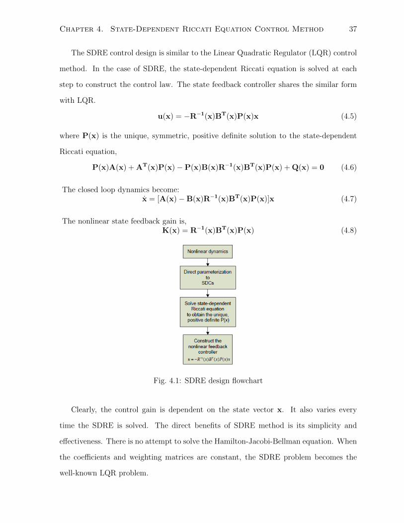
The SDRE control design is similar to the Linear Quadratic Regulator (LQR) control
method. In the case of SDRE, the state-dependent Riccati equation is solved at each
step to construct the control law. The state feedback controller shares the similar form
with LQR.
u(x) = −R−1(x)BT(x)P(x)x (4.5)
where P(x) is the unique, symmetric, positive definite solution to the state-dependent
Riccati equation,
P(x)A(x) + AT(x)P(x)−P(x)B(x)R−1(x)BT(x)P(x) + Q(x) = 0 (4.6)
The closed loop dynamics become:x = [A(x)−B(x)R−1(x)BT(x)P(x)]x (4.7)
The nonlinear state feedback gain is,K(x) = R−1(x)BT(x)P(x) (4.8)
Fig. 4.1: SDRE design flowchart
Clearly, the control gain is dependent on the state vector x. It also varies every
time the SDRE is solved. The direct benefits of SDRE method is its simplicity and
effectiveness. There is no attempt to solve the Hamilton-Jacobi-Bellman equation. When
the coefficients and weighting matrices are constant, the SDRE problem becomes the
well-known LQR problem.
Chapter 4. State-Dependent Riccati Equation Control Method 38
Fig. 4.1 shows the systematic procedures to construct the nonlinear state feedback
gain with the SDRE control method.
4.2 Stability and Optimality Analysis
4.2.1 Stability Analysis
Stability is an important issue for any controller. Nonlinear system stability is well
defined by the Lyapunov stability theories [27]. Although global asymptotic stability
of the closed-loop system is highly desirable, such a property is difficult to achieve and
prove. In the case of SDRE control method, global asymptotic stability can only be
proved in two special cases. In the first case, the closed-loop coefficient matrix ACL(x)
is assumed to possess a special structure. The second case involved the single system
state, n = 1. Despite the difficulty to prove the global asymptotic stability property, the
local asymptotic stability is well proven [10] and presented here.
Theorem 1. [39] Consider the nonlinear multivaribale system Eq.(4.1) with feedback
control Eq.(4.5) applied where x ∈ <n (n > 1) and P(x) is the unique, symmetric,
positive-definite, pointwise-stabilizing solution of the SDRE Eq.(4.6). Then, under As-
sumptions 3 and 4, the SDRE method produces a closed-loop solution which is locall
asymptotically stable
Proof. Using SDRE control, the closed-loop solution becomes x = ACL(x)x, where
ACL(x) is the closed-loop SDC matrix. From Riccati equation theory, ACL(x) is guar-
anteed to be stable at every point x. Under the smoothness assumptions of Assumption
4, P(x) is continuously differentiable and hence so is ACL(x). Applying the Mean Value
Theorem to ACL(x) gives,
ACL(x) = ACL(0) +∂ACL(z)
∂xx (4.9)
where ∂ACL(z)∂x
generates a tensor, and the vector z is that point on the line segment
Chapter 4. State-Dependent Riccati Equation Control Method 39
joining the origin 0 and x. As a result,
x = ACL(x)x (4.10)
x = (ACL(0) +∂ACL(z)
∂xx)x (4.11)
x = ACL(0)x + xT∂ACL(z)
∂xx (4.12)
which gives,
x = ACL(0)x + ψ(x, z) ‖x‖ (4.13)
where ψ(x, z) = 1‖x‖x
T ∂ACL(z)∂x
x, such that lim‖x‖→0 ψ(x, z) = 0. Hence, in a neighbor-
hood about the origin, the linear term which has a constant stable coefficient matrix
ACL(0) dominates the higher-order terms, yielding the local asymptotic stability.
In the case of global asymptotic stability property, the following two Theorems apply,
Theorem 2. [12] If the closed-loop coefficient matrix ACL(x) is symmetric for all
x, then under the conditions given by the Assumptions 4 and 5, the SDRE closed-loop
solution is global asymptotically stable.
Theorem 3. In the scalar case (n=1), the SDRE closed-loop solution is globally asymp-
totically stable.
The proofs of the above Theorem can be found in the Cloutier et al. [12].
4.2.2 Optimality Analysis
The SDRE control method is often regarded as a sub-optimal nonlinear control method.
In this subsection, the optimality property of the SDRE method is addressed.
Assumption 5. A(x), B(x), P(x), Q(x) and R(x) along with their gradients ∂A(x)∂x
,
∂B(x)∂x
, ∂P(x)∂x
, ∂Q(x)∂x
, ∂R(x)∂x
are bounded in a neighborhood Ω about the origin.
Chapter 4. State-Dependent Riccati Equation Control Method 40
Theorem 4. [39] In the general multivariable case (n > 1), the SDRE nonlinear feed-
back solution and its associated state and costate trajectories satisfy the first necessary
condition for optimality (∂H∂u
= 0) of the nonlinear optimal regulator problem Eq.(4.1)
and Eq.(4.2), where H is the Hamiltonian of the system. Additionally, if Assumption 5
holds, under asymptotic stability, as the state x is driven to zero, the second necessary
condition for optimality λ = −∂H∂x
is asymptotically satisfied at a quadratic rate.
The proof is available in the work of Mracek et al. [39]. Theorem 4 shows the sub-
optimality property of the SDRE control method. As the Theorem states, the second
condition for optimality is only satisfied asymptotically. However, similar to the stability
property, SDRE global optimality property is possible under special circumstances [7],
such as in the scalar case.
4.3 The Art and Capabilities of SDRE
The SDRE controller design provides an effective and systematic way to construct the
nonlinear controller. It also offers great design flexibility to the designer via state-
dependent matrices. In this section, some of the important SDRE design techniques
and their capabilities are covered. In order to implement the SDRE method, the sys-
tem must conform to the SDRE design requirements. In this case, the system must be
affinity-in-control and f(0) = 0. In this section, the techniques are also introduced to
deal with non-conforming nonlinear systems so that the SDRE control method can still
be applied to such systems. These concepts and techniques are implemented in the sim-
ulation examples to demonstrate the design approach, controller performance as well as
their promising results.
Design Freedom
One of the main advantages of the SDRE method is the design freedom, which is via
the state-dependent coefficients to capture system nonlinearity. The parameterization is
Chapter 4. State-Dependent Riccati Equation Control Method 41
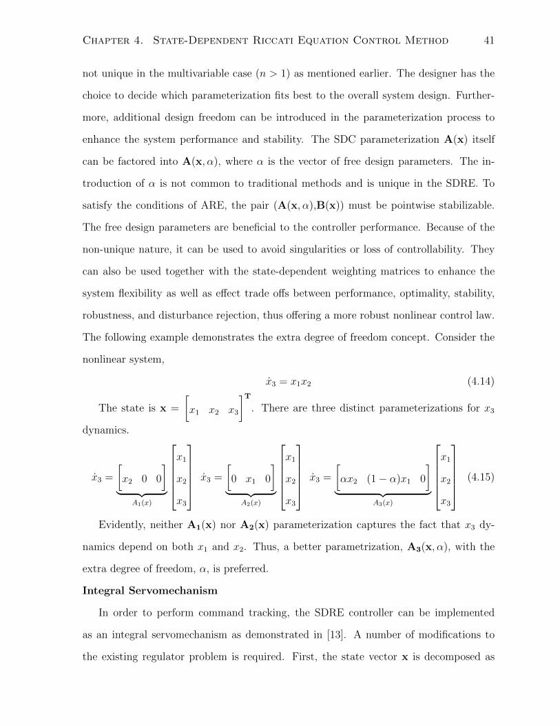
not unique in the multivariable case (n > 1) as mentioned earlier. The designer has the
choice to decide which parameterization fits best to the overall system design. Further-
more, additional design freedom can be introduced in the parameterization process to
enhance the system performance and stability. The SDC parameterization A(x) itself
can be factored into A(x, α), where α is the vector of free design parameters. The in-
troduction of α is not common to traditional methods and is unique in the SDRE. To
satisfy the conditions of ARE, the pair (A(x, α),B(x)) must be pointwise stabilizable.
The free design parameters are beneficial to the controller performance. Because of the
non-unique nature, it can be used to avoid singularities or loss of controllability. They
can also be used together with the state-dependent weighting matrices to enhance the
system flexibility as well as effect trade offs between performance, optimality, stability,
robustness, and disturbance rejection, thus offering a more robust nonlinear control law.
The following example demonstrates the extra degree of freedom concept. Consider the
nonlinear system,
x3 = x1x2 (4.14)
The state is x =
[x1 x2 x3
]T. There are three distinct parameterizations for x3
dynamics.
x3 =
[x2 0 0
]︸ ︷︷ ︸
A1(x)
x1
x2
x3
x3 =
[0 x1 0
]︸ ︷︷ ︸
A2(x)
x1
x2
x3
x3 =
[αx2 (1− α)x1 0
]︸ ︷︷ ︸
A3(x)
x1
x2
x3
(4.15)
Evidently, neither A1(x) nor A2(x) parameterization captures the fact that x3 dy-
namics depend on both x1 and x2. Thus, a better parametrization, A3(x, α), with the
extra degree of freedom, α, is preferred.
Integral Servomechanism
In order to perform command tracking, the SDRE controller can be implemented
as an integral servomechanism as demonstrated in [13]. A number of modifications to
the existing regulator problem is required. First, the state vector x is decomposed as
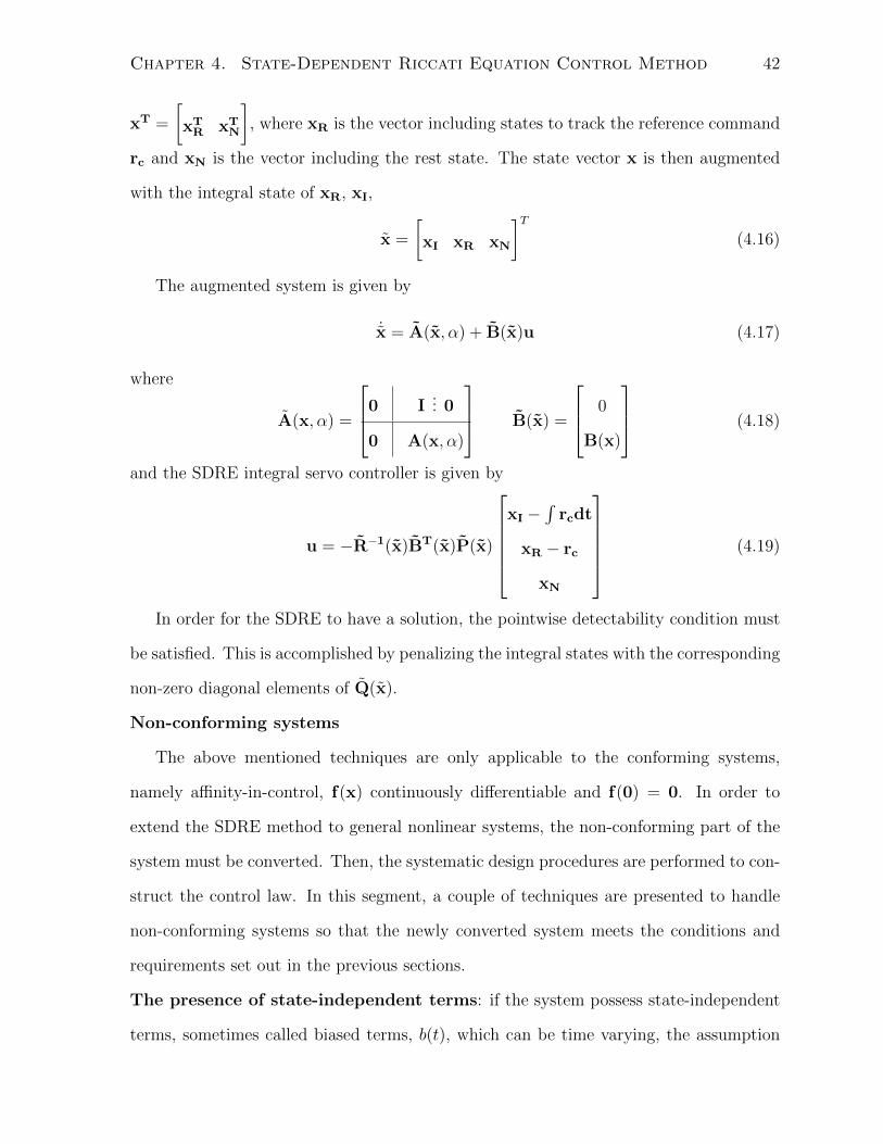
Chapter 4. State-Dependent Riccati Equation Control Method 42
xT =
[xTR xT
N
], where xR is the vector including states to track the reference command
rc and xN is the vector including the rest state. The state vector x is then augmented
with the integral state of xR, xI,
x =
[xI xR xN
]T(4.16)
The augmented system is given by
˙x = A(x, α) + B(x)u (4.17)
where
A(x, α) =
0 I... 0
0 A(x, α)
B(x) =
0
B(x)
(4.18)
and the SDRE integral servo controller is given by
u = −R−1(x)BT(x)P(x)
xI −
∫rcdt
xR − rc
xN
(4.19)
In order for the SDRE to have a solution, the pointwise detectability condition must
be satisfied. This is accomplished by penalizing the integral states with the corresponding
non-zero diagonal elements of Q(x).
Non-conforming systems
The above mentioned techniques are only applicable to the conforming systems,
namely affinity-in-control, f(x) continuously differentiable and f(0) = 0. In order to
extend the SDRE method to general nonlinear systems, the non-conforming part of the
system must be converted. Then, the systematic design procedures are performed to con-
struct the control law. In this segment, a couple of techniques are presented to handle
non-conforming systems so that the newly converted system meets the conditions and
requirements set out in the previous sections.
The presence of state-independent terms: if the system possess state-independent
terms, sometimes called biased terms, b(t), which can be time varying, the assumption
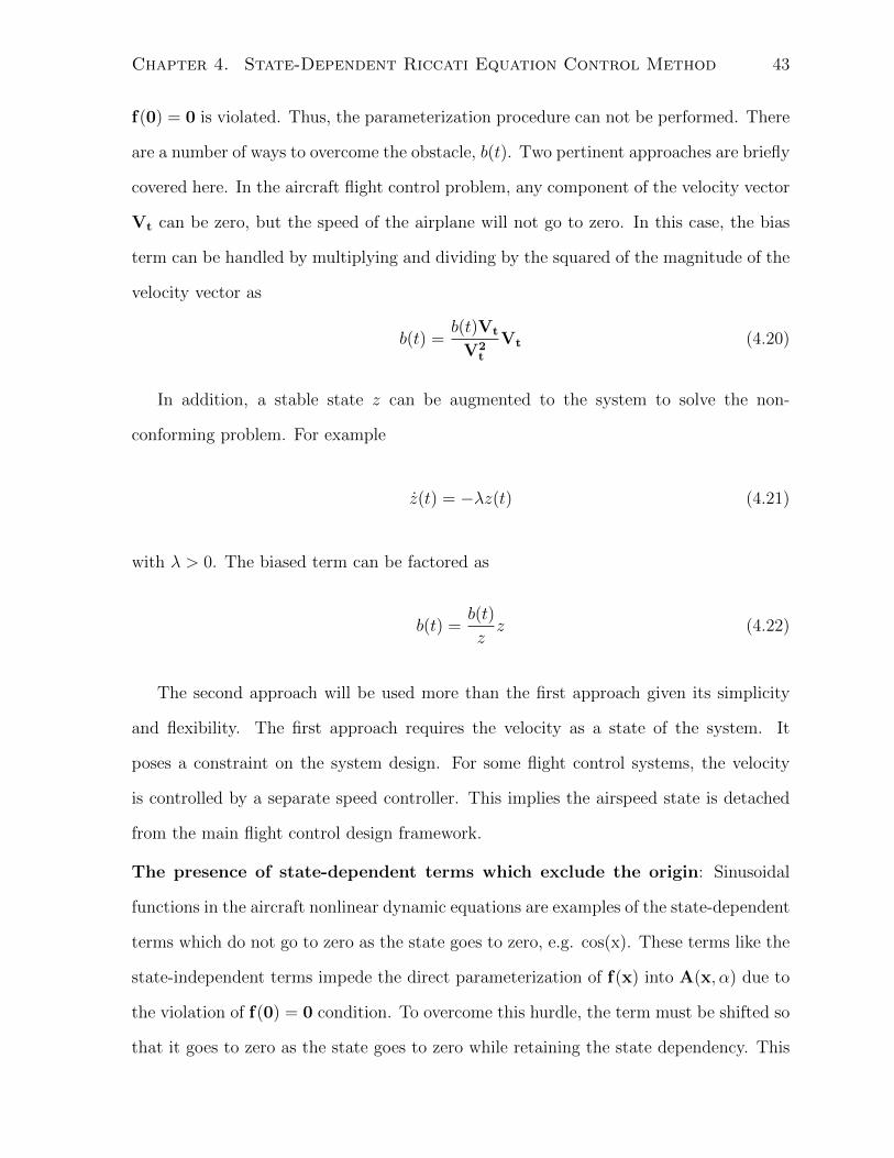
Chapter 4. State-Dependent Riccati Equation Control Method 43
f(0) = 0 is violated. Thus, the parameterization procedure can not be performed. There
are a number of ways to overcome the obstacle, b(t). Two pertinent approaches are briefly
covered here. In the aircraft flight control problem, any component of the velocity vector
Vt can be zero, but the speed of the airplane will not go to zero. In this case, the bias
term can be handled by multiplying and dividing by the squared of the magnitude of the
velocity vector as
b(t) =b(t)Vt
V2t
Vt (4.20)
In addition, a stable state z can be augmented to the system to solve the non-
conforming problem. For example
z(t) = −λz(t) (4.21)
with λ > 0. The biased term can be factored as
b(t) =b(t)
zz (4.22)
The second approach will be used more than the first approach given its simplicity
and flexibility. The first approach requires the velocity as a state of the system. It
poses a constraint on the system design. For some flight control systems, the velocity
is controlled by a separate speed controller. This implies the airspeed state is detached
from the main flight control design framework.
The presence of state-dependent terms which exclude the origin: Sinusoidal
functions in the aircraft nonlinear dynamic equations are examples of the state-dependent
terms which do not go to zero as the state goes to zero, e.g. cos(x). These terms like the
state-independent terms impede the direct parameterization of f(x) into A(x, α) due to
the violation of f(0) = 0 condition. To overcome this hurdle, the term must be shifted so
that it goes to zero as the state goes to zero while retaining the state dependency. This
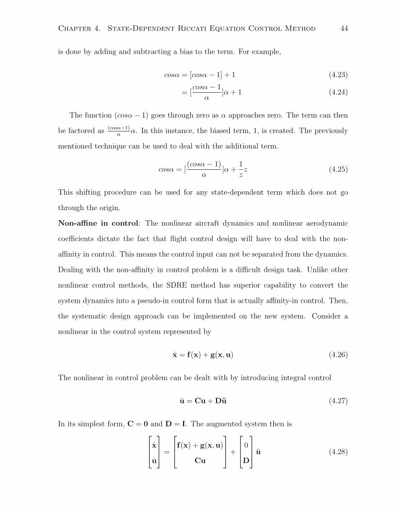
Chapter 4. State-Dependent Riccati Equation Control Method 44
is done by adding and subtracting a bias to the term. For example,
cosα = [cosα− 1] + 1 (4.23)
= [cosα− 1
α]α + 1 (4.24)
The function (cosα− 1) goes through zero as α approaches zero. The term can then
be factored as (cosα−1)α
α. In this instance, the biased term, 1, is created. The previously
mentioned technique can be used to deal with the additional term.
cosα = [(cosα− 1)
α]α +
1
zz (4.25)
This shifting procedure can be used for any state-dependent term which does not go
through the origin.
Non-affine in control: The nonlinear aircraft dynamics and nonlinear aerodynamic
coefficients dictate the fact that flight control design will have to deal with the non-
affinity in control. This means the control input can not be separated from the dynamics.
Dealing with the non-affinity in control problem is a difficult design task. Unlike other
nonlinear control methods, the SDRE method has superior capability to convert the
system dynamics into a pseudo-in control form that is actually affinity-in control. Then,
the systematic design approach can be implemented on the new system. Consider a
nonlinear in the control system represented by
x = f(x) + g(x,u) (4.26)
The nonlinear in control problem can be dealt with by introducing integral control
u = Cu + Du (4.27)
In its simplest form, C = 0 and D = I. The augmented system then isx
u
=
f(x) + g(x,u)
Cu
+
0
D
u (4.28)
Chapter 4. State-Dependent Riccati Equation Control Method 45
which is affine in control. The above mentioned techniques can also be implemented in
the case that the system does not conform with the required structure. Direct parame-
terization can then be performed.
Numerical SDC: It is worth mentioning that in addition to analytical parameterization
to obtain the state-dependent coefficients, the numerical approach is also available to
perform the task. The idea is based on the perturbation of the state control vectors. The
approach is fully described in Menon et al.’s work [34].
4.4 Simulation Studies
This section focuses on the simulation studies of the guidance and SDRE flight system
framework. The framework is tested with two different damaged aircraft scenarios. The
SDRE method is implemented as the flight control law while the zero effort miss vec-
tor provides the guidance commands. In Chapter 2, Table 2.1 a list of damage cases
investigated in the work is given. In this section, only the loss-of-thrust and the eleva-
tor ineffectiveness cases are considered. The complete loss-of-thrust in flight forces the
aircraft to become a glider in the air. Any error in the calculation of the distance, and
maneuver to the nearest approachable runway can be catastrophic since the allowable
error margin is very small. In this example, the SDRE controller actively reconfigures
itself to accommodate the guidance commands and the aircraft impaired dynamics.
In the case of actuator damage, a complete flight control system with the speed
controller is designed and simulated. The flight control system consists of three loops:
the inner loop, the outer loop and the flight path angle loop as described in the previous
chapter. Similar to the loss-of-thrust example, the SDRE control law is also able to deal
with the aircraft behaviors change while maintaining the command tracking.
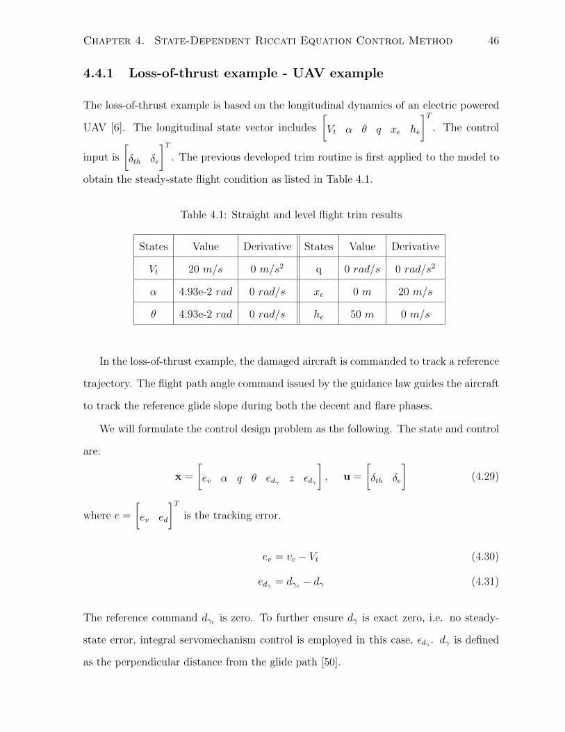
Chapter 4. State-Dependent Riccati Equation Control Method 46
4.4.1 Loss-of-thrust example - UAV example
The loss-of-thrust example is based on the longitudinal dynamics of an electric powered
UAV [6]. The longitudinal state vector includes
[Vt α θ q xe he
]T. The control
input is
[δth δe
]T. The previous developed trim routine is first applied to the model to
obtain the steady-state flight condition as listed in Table 4.1.
Table 4.1: Straight and level flight trim results
States Value Derivative States Value Derivative
Vt 20 m/s 0 m/s2 q 0 rad/s 0 rad/s2
α 4.93e-2 rad 0 rad/s xe 0 m 20 m/s
θ 4.93e-2 rad 0 rad/s he 50 m 0 m/s
In the loss-of-thrust example, the damaged aircraft is commanded to track a reference
trajectory. The flight path angle command issued by the guidance law guides the aircraft
to track the reference glide slope during both the decent and flare phases.
We will formulate the control design problem as the following. The state and control
are:
x =
[ev α q θ edγ z εdγ
], u =
[δth δe
](4.29)
where e =
[ev ed
]Tis the tracking error.
ev = vc − Vt (4.30)
edγ = dγc − dγ (4.31)
The reference command dγc is zero. To further ensure dγ is exact zero, i.e. no steady-
state error, integral servomechanism control is employed in this case, εdγ . dγ is defined
as the perpendicular distance from the glide path [50].
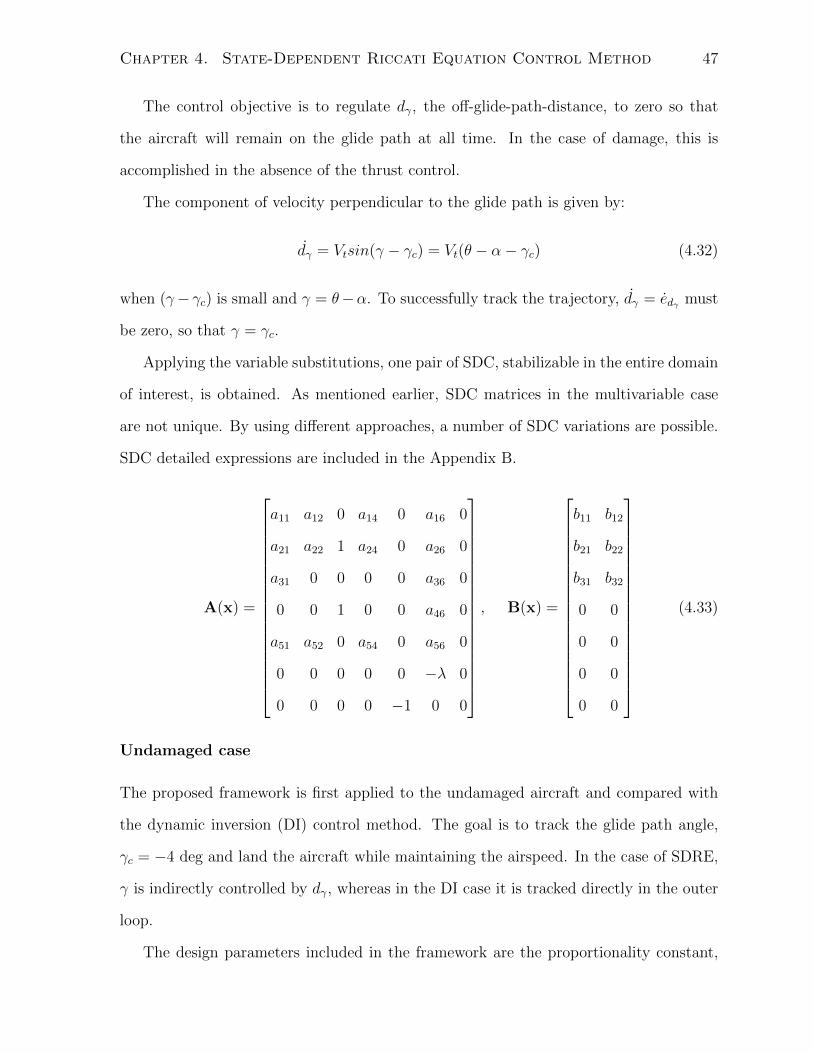
Chapter 4. State-Dependent Riccati Equation Control Method 47
The control objective is to regulate dγ, the off-glide-path-distance, to zero so that
the aircraft will remain on the glide path at all time. In the case of damage, this is
accomplished in the absence of the thrust control.
The component of velocity perpendicular to the glide path is given by:
dγ = Vtsin(γ − γc) = Vt(θ − α− γc) (4.32)
when (γ− γc) is small and γ = θ−α. To successfully track the trajectory, dγ = edγ must
be zero, so that γ = γc.
Applying the variable substitutions, one pair of SDC, stabilizable in the entire domain
of interest, is obtained. As mentioned earlier, SDC matrices in the multivariable case
are not unique. By using different approaches, a number of SDC variations are possible.
SDC detailed expressions are included in the Appendix B.
A(x) =
a11 a12 0 a14 0 a16 0
a21 a22 1 a24 0 a26 0
a31 0 0 0 0 a36 0
0 0 1 0 0 a46 0
a51 a52 0 a54 0 a56 0
0 0 0 0 0 −λ 0
0 0 0 0 −1 0 0
, B(x) =
b11 b12
b21 b22
b31 b32
0 0
0 0
0 0
0 0
(4.33)
Undamaged case
The proposed framework is first applied to the undamaged aircraft and compared with
the dynamic inversion (DI) control method. The goal is to track the glide path angle,
γc = −4 deg and land the aircraft while maintaining the airspeed. In the case of SDRE,
γ is indirectly controlled by dγ, whereas in the DI case it is tracked directly in the outer
loop.
The design parameters included in the framework are the proportionality constant,
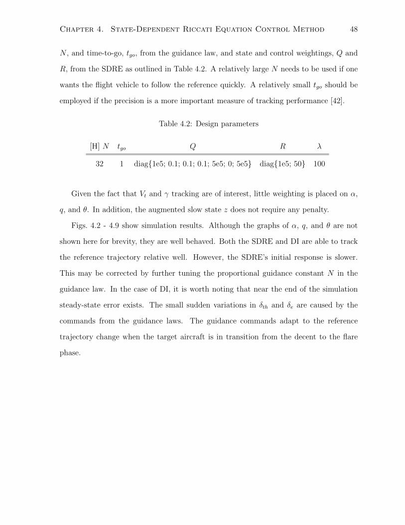
Chapter 4. State-Dependent Riccati Equation Control Method 48
N , and time-to-go, tgo, from the guidance law, and state and control weightings, Q and
R, from the SDRE as outlined in Table 4.2. A relatively large N needs to be used if one
wants the flight vehicle to follow the reference quickly. A relatively small tgo should be
employed if the precision is a more important measure of tracking performance [42].
Table 4.2: Design parameters
[H] N tgo Q R λ
32 1 diag1e5; 0.1; 0.1; 0.1; 5e5; 0; 5e5 diag1e5; 50 100
Given the fact that Vt and γ tracking are of interest, little weighting is placed on α,
q, and θ. In addition, the augmented slow state z does not require any penalty.
Figs. 4.2 - 4.9 show simulation results. Although the graphs of α, q, and θ are not
shown here for brevity, they are well behaved. Both the SDRE and DI are able to track
the reference trajectory relative well. However, the SDRE’s initial response is slower.
This may be corrected by further tuning the proportional guidance constant N in the
guidance law. In the case of DI, it is worth noting that near the end of the simulation
steady-state error exists. The small sudden variations in δth and δe are caused by the
commands from the guidance laws. The guidance commands adapt to the reference
trajectory change when the target aircraft is in transition from the decent to the flare
phase.
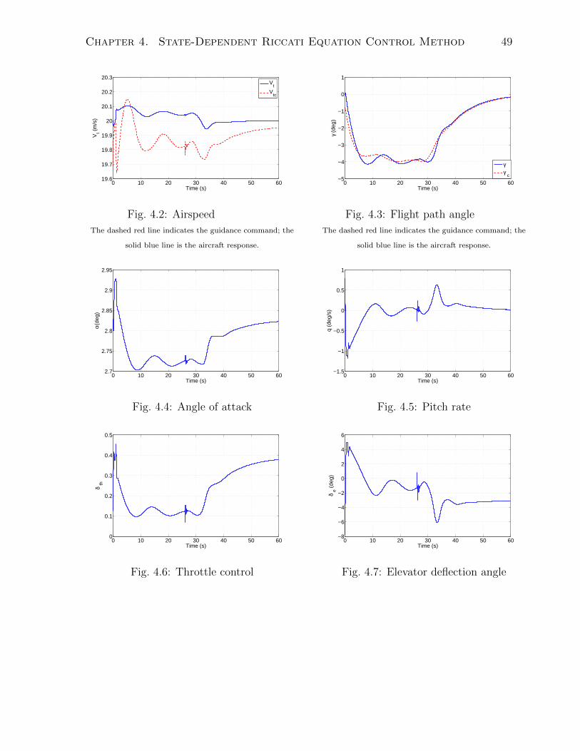
Chapter 4. State-Dependent Riccati Equation Control Method 49
0 10 20 30 40 50 6019.6
19.7
19.8
19.9
20
20.1
20.2
20.3
Time (s)
Vt (
m/s
)
Vt
Vtc
Fig. 4.2: Airspeed
The dashed red line indicates the guidance command; the
solid blue line is the aircraft response.
0 10 20 30 40 50 60−5
−4
−3
−2
−1
0
1
Time (s)
γ (d
eg)
γγ
c
Fig. 4.3: Flight path angle
The dashed red line indicates the guidance command; the
solid blue line is the aircraft response.
0 10 20 30 40 50 602.7
2.75
2.8
2.85
2.9
2.95
Time (s)
α(de
g)
Fig. 4.4: Angle of attack
0 10 20 30 40 50 60−1.5
−1
−0.5
0
0.5
1
Time (s)
q (d
eg/s
)
Fig. 4.5: Pitch rate
0 10 20 30 40 50 600
0.1
0.2
0.3
0.4
0.5
Time (s)
δ th
Fig. 4.6: Throttle control
0 10 20 30 40 50 60−8
−6
−4
−2
0
2
4
6
Time (s)
δ e (
deg)
Fig. 4.7: Elevator deflection angle
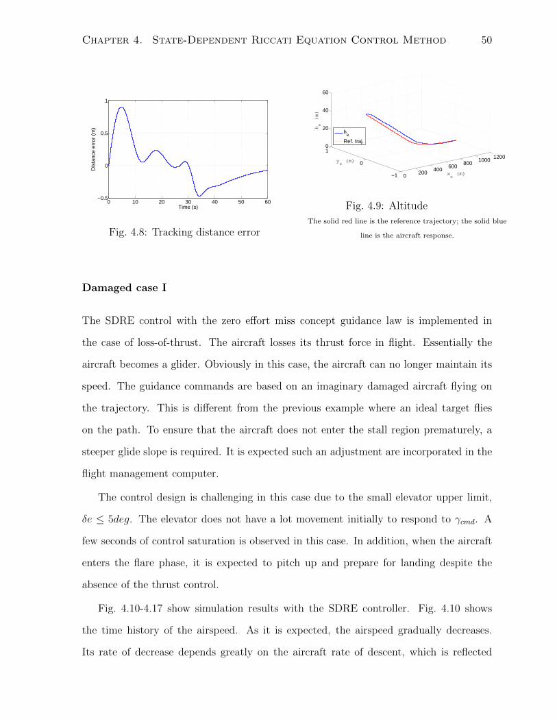
Chapter 4. State-Dependent Riccati Equation Control Method 50
0 10 20 30 40 50 60−0.5
0
0.5
1
Time (s)
Dis
tanc
e er
ror
(m)
Fig. 4.8: Tracking distance error
0200
400600
8001000
1200
−1
0
10
20
40
60
xe (m)
ye (m)
he (m)
he
Ref. traj.
Fig. 4.9: Altitude
The solid red line is the reference trajectory; the solid blue
line is the aircraft response.
Damaged case I
The SDRE control with the zero effort miss concept guidance law is implemented in
the case of loss-of-thrust. The aircraft losses its thrust force in flight. Essentially the
aircraft becomes a glider. Obviously in this case, the aircraft can no longer maintain its
speed. The guidance commands are based on an imaginary damaged aircraft flying on
the trajectory. This is different from the previous example where an ideal target flies
on the path. To ensure that the aircraft does not enter the stall region prematurely, a
steeper glide slope is required. It is expected such an adjustment are incorporated in the
flight management computer.
The control design is challenging in this case due to the small elevator upper limit,
δe ≤ 5deg. The elevator does not have a lot movement initially to respond to γcmd. A
few seconds of control saturation is observed in this case. In addition, when the aircraft
enters the flare phase, it is expected to pitch up and prepare for landing despite the
absence of the thrust control.
Fig. 4.10-4.17 show simulation results with the SDRE controller. Fig. 4.10 shows
the time history of the airspeed. As it is expected, the airspeed gradually decreases.
Its rate of decrease depends greatly on the aircraft rate of descent, which is reflected
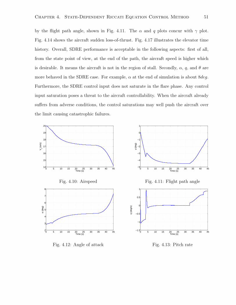
Chapter 4. State-Dependent Riccati Equation Control Method 51
by the flight path angle, shown in Fig. 4.11. The α and q plots concur with γ plot.
Fig. 4.14 shows the aircraft sudden loss-of-thrust. Fig. 4.17 illustrates the elevator time
history. Overall, SDRE performance is acceptable in the following aspects: first of all,
from the state point of view, at the end of the path, the aircraft speed is higher which
is desirable. It means the aircraft is not in the region of stall. Secondly, α, q, and θ are
more behaved in the SDRE case. For example, α at the end of simulation is about 8deg.
Furthermore, the SDRE control input does not saturate in the flare phase. Any control
input saturation poses a threat to the aircraft controllability. When the aircraft already
suffers from adverse conditions, the control saturations may well push the aircraft over
the limit causing catastrophic failures.
0 5 10 15 20 25 30 35 40 4514
15
16
17
18
19
20
Time (s)
Vt (
m/s
)
Fig. 4.10: Airspeed
0 5 10 15 20 25 30 35 40 45−5
−4
−3
−2
−1
0
1
Time (s)
γ (d
eg)
Fig. 4.11: Flight path angle
0 5 10 15 20 25 30 35 40 452
3
4
5
6
7
8
Time (s)
α (d
eg)
Fig. 4.12: Angle of attack
0 5 10 15 20 25 30 35 40 45−1.5
−1
−0.5
0
0.5
1
Time (s)
q (d
eg/s
)
Fig. 4.13: Pitch rate
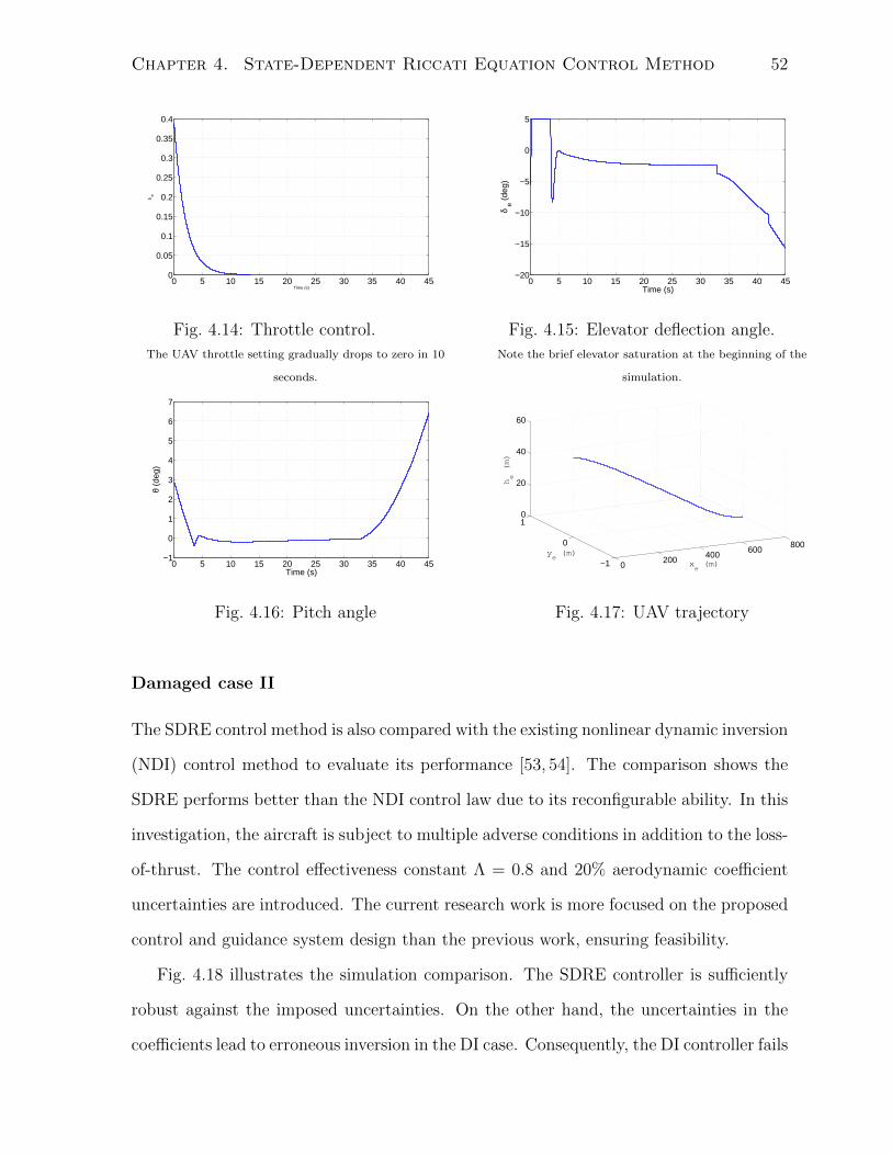
Chapter 4. State-Dependent Riccati Equation Control Method 52
0 5 10 15 20 25 30 35 40 450
0.05
0.1
0.15
0.2
0.25
0.3
0.35
0.4
Time (s)
δ th
Fig. 4.14: Throttle control.
The UAV throttle setting gradually drops to zero in 10
seconds.
0 5 10 15 20 25 30 35 40 45−20
−15
−10
−5
0
5
Time (s)
δ e (
deg)
Fig. 4.15: Elevator deflection angle.
Note the brief elevator saturation at the beginning of the
simulation.
0 5 10 15 20 25 30 35 40 45−1
0
1
2
3
4
5
6
7
Time (s)
θ (d
eg)
Fig. 4.16: Pitch angle
0200
400600
800
−1
0
10
20
40
60
xe (m)
ye (m)
he (m)
Fig. 4.17: UAV trajectory
Damaged case II
The SDRE control method is also compared with the existing nonlinear dynamic inversion
(NDI) control method to evaluate its performance [53, 54]. The comparison shows the
SDRE performs better than the NDI control law due to its reconfigurable ability. In this
investigation, the aircraft is subject to multiple adverse conditions in addition to the loss-
of-thrust. The control effectiveness constant Λ = 0.8 and 20% aerodynamic coefficient
uncertainties are introduced. The current research work is more focused on the proposed
control and guidance system design than the previous work, ensuring feasibility.
Fig. 4.18 illustrates the simulation comparison. The SDRE controller is sufficiently
robust against the imposed uncertainties. On the other hand, the uncertainties in the
coefficients lead to erroneous inversion in the DI case. Consequently, the DI controller fails
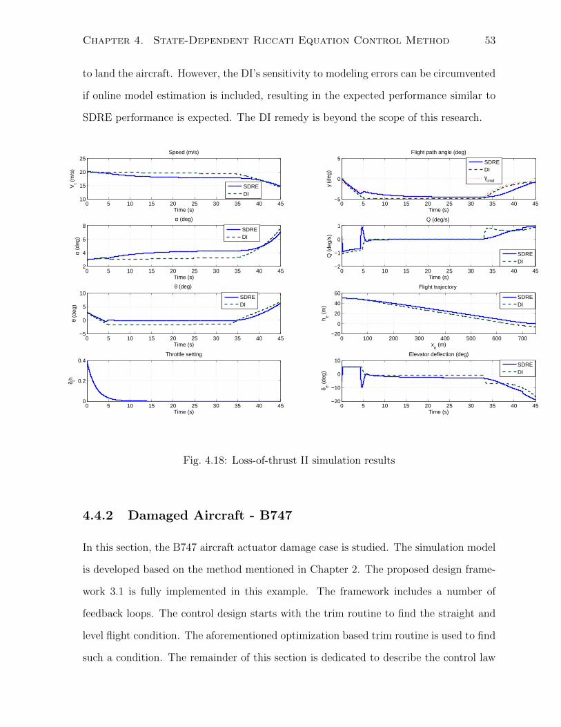
Chapter 4. State-Dependent Riccati Equation Control Method 53
to land the aircraft. However, the DI’s sensitivity to modeling errors can be circumvented
if online model estimation is included, resulting in the expected performance similar to
SDRE performance is expected. The DI remedy is beyond the scope of this research.
0 5 10 15 20 25 30 35 40 4510
15
20
25Speed (m/s)
Time (s)
Vt (
m/s
)
0 5 10 15 20 25 30 35 40 45−5
0
5Flight path angle (deg)
Time (s)
γ (d
eg)
0 5 10 15 20 25 30 35 40 452
4
6
8α (deg)
Time (s)
α (d
eg)
0 5 10 15 20 25 30 35 40 45−2
−1
0
1Q (deg/s)
Time (s)
Q (
deg/
s)
0 5 10 15 20 25 30 35 40 45−5
0
5
10θ (deg)
Time (s)
θ (d
eg)
0 100 200 300 400 500 600 700−20
0
20
40
60Flight trajectory
xe (m)
h e (m
)
0 5 10 15 20 25 30 35 40 450
0.2
0.4Throttle setting
Time (s)
δ th
0 5 10 15 20 25 30 35 40 45−20
−10
0
10Elevator deflection (deg)
Time (s)
δ e (de
g)
SDREDI
SDREDI
SDREDI
SDREDIγcmd
SDREDI
SDREDI
SDREDI
Fig. 4.18: Loss-of-thrust II simulation results
4.4.2 Damaged Aircraft - B747
In this section, the B747 aircraft actuator damage case is studied. The simulation model
is developed based on the method mentioned in Chapter 2. The proposed design frame-
work 3.1 is fully implemented in this example. The framework includes a number of
feedback loops. The control design starts with the trim routine to find the straight and
level flight condition. The aforementioned optimization based trim routine is used to find
such a condition. The remainder of this section is dedicated to describe the control law
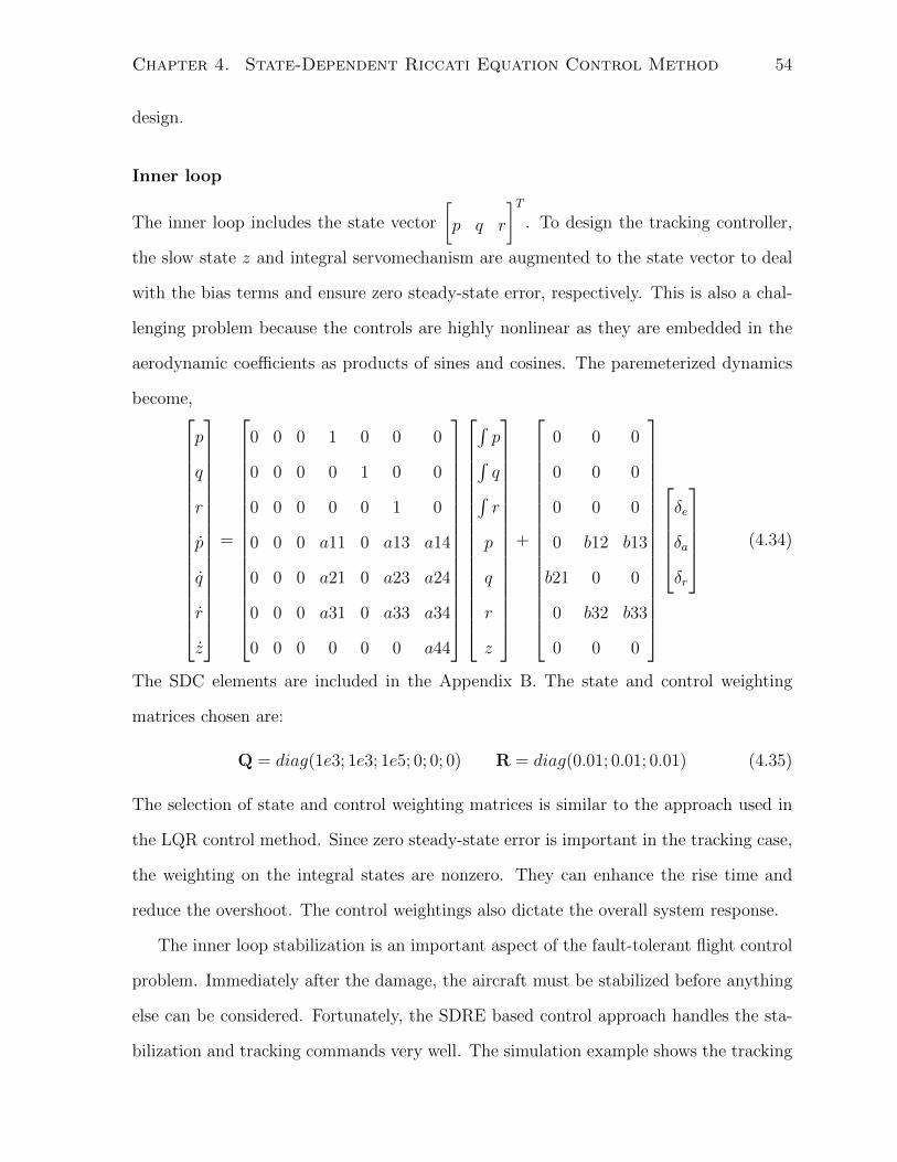
Chapter 4. State-Dependent Riccati Equation Control Method 54
design.
Inner loop
The inner loop includes the state vector
[p q r
]T. To design the tracking controller,
the slow state z and integral servomechanism are augmented to the state vector to deal
with the bias terms and ensure zero steady-state error, respectively. This is also a chal-
lenging problem because the controls are highly nonlinear as they are embedded in the
aerodynamic coefficients as products of sines and cosines. The paremeterized dynamics
become,
p
q
r
p
q
r
z
=
0 0 0 1 0 0 0
0 0 0 0 1 0 0
0 0 0 0 0 1 0
0 0 0 a11 0 a13 a14
0 0 0 a21 0 a23 a24
0 0 0 a31 0 a33 a34
0 0 0 0 0 0 a44
∫p∫q∫r
p
q
r
z
+
0 0 0
0 0 0
0 0 0
0 b12 b13
b21 0 0
0 b32 b33
0 0 0
δe
δa
δr
(4.34)
The SDC elements are included in the Appendix B. The state and control weighting
matrices chosen are:
Q = diag(1e3; 1e3; 1e5; 0; 0; 0) R = diag(0.01; 0.01; 0.01) (4.35)
The selection of state and control weighting matrices is similar to the approach used in
the LQR control method. Since zero steady-state error is important in the tracking case,
the weighting on the integral states are nonzero. They can enhance the rise time and
reduce the overshoot. The control weightings also dictate the overall system response.
The inner loop stabilization is an important aspect of the fault-tolerant flight control
problem. Immediately after the damage, the aircraft must be stabilized before anything
else can be considered. Fortunately, the SDRE based control approach handles the sta-
bilization and tracking commands very well. The simulation example shows the tracking
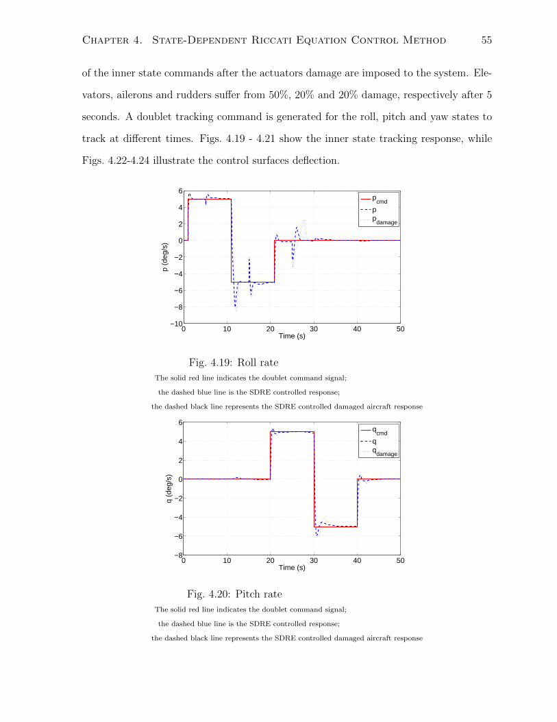
Chapter 4. State-Dependent Riccati Equation Control Method 55
of the inner state commands after the actuators damage are imposed to the system. Ele-
vators, ailerons and rudders suffer from 50%, 20% and 20% damage, respectively after 5
seconds. A doublet tracking command is generated for the roll, pitch and yaw states to
track at different times. Figs. 4.19 - 4.21 show the inner state tracking response, while
Figs. 4.22-4.24 illustrate the control surfaces deflection.
0 10 20 30 40 50−10
−8
−6
−4
−2
0
2
4
6
Time (s)
p (d
eg/s
)
pcmd
pp
damage
Fig. 4.19: Roll rate
The solid red line indicates the doublet command signal;
the dashed blue line is the SDRE controlled response;
the dashed black line represents the SDRE controlled damaged aircraft response
0 10 20 30 40 50−8
−6
−4
−2
0
2
4
6
Time (s)
q (d
eg/s
)
qcmd
damage
Fig. 4.20: Pitch rate
The solid red line indicates the doublet command signal;
the dashed blue line is the SDRE controlled response;
the dashed black line represents the SDRE controlled damaged aircraft response
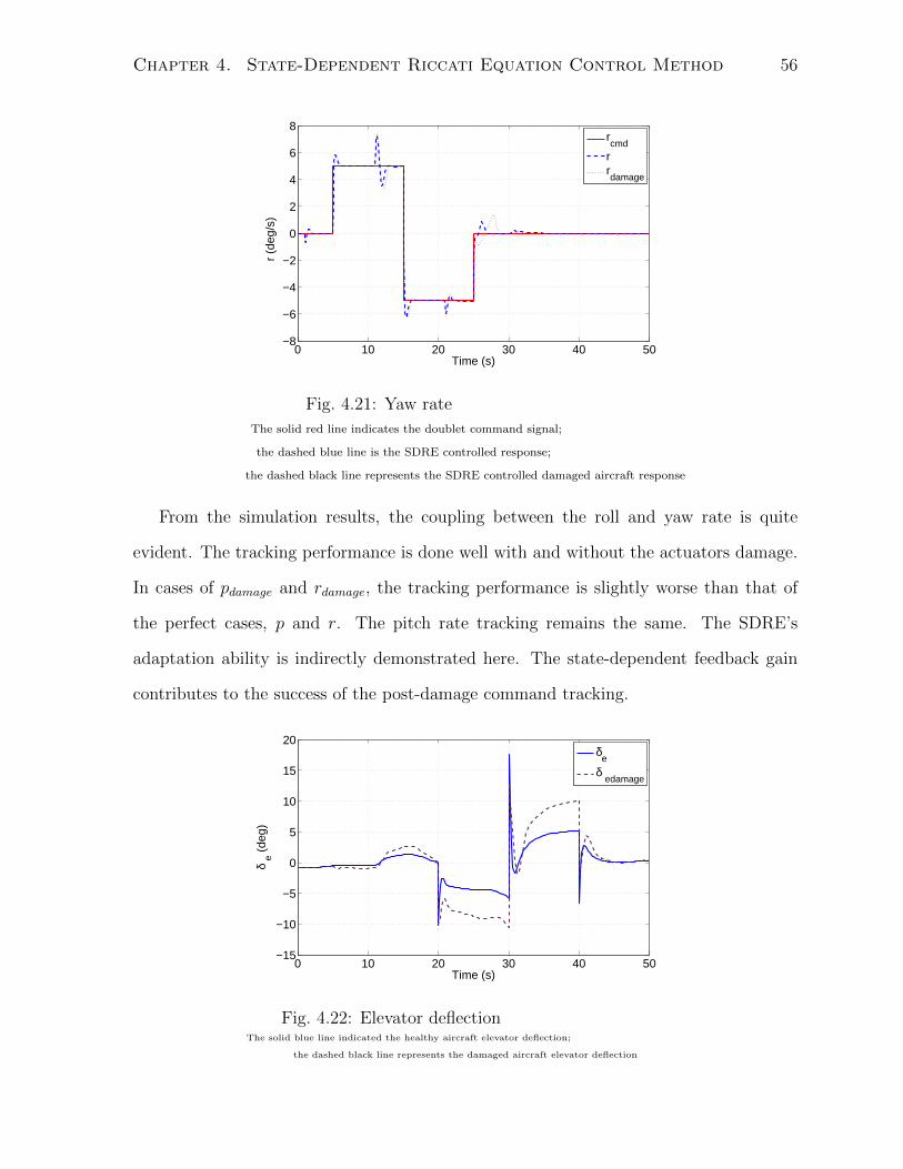
Chapter 4. State-Dependent Riccati Equation Control Method 56
0 10 20 30 40 50−8
−6
−4
−2
0
2
4
6
8
Time (s)
r (d
eg/s
)
rcmd
rrdamage
Fig. 4.21: Yaw rate
The solid red line indicates the doublet command signal;
the dashed blue line is the SDRE controlled response;
the dashed black line represents the SDRE controlled damaged aircraft response
From the simulation results, the coupling between the roll and yaw rate is quite
evident. The tracking performance is done well with and without the actuators damage.
In cases of pdamage and rdamage, the tracking performance is slightly worse than that of
the perfect cases, p and r. The pitch rate tracking remains the same. The SDRE’s
adaptation ability is indirectly demonstrated here. The state-dependent feedback gain
contributes to the success of the post-damage command tracking.
0 10 20 30 40 50−15
−10
−5
0
5
10
15
20
Time (s)
δ e (
deg)
δe
δ edamage
Fig. 4.22: Elevator deflectionThe solid blue line indicated the healthy aircraft elevator deflection;
the dashed black line represents the damaged aircraft elevator deflection
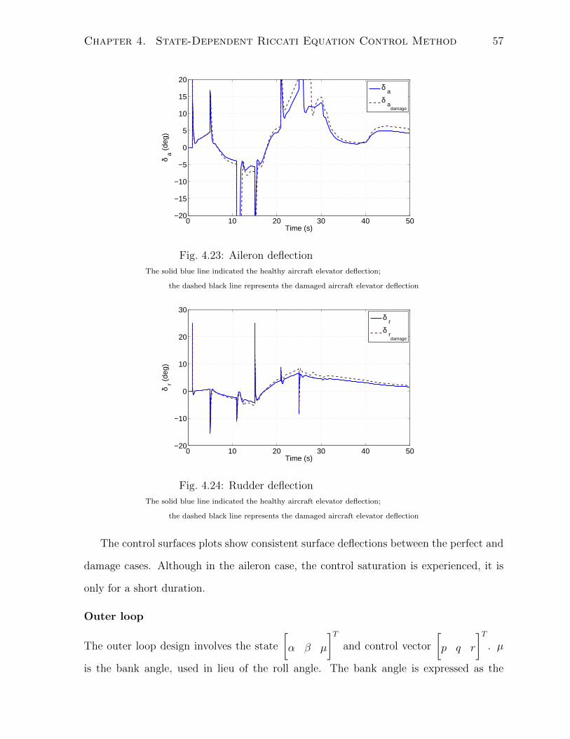
Chapter 4. State-Dependent Riccati Equation Control Method 57
0 10 20 30 40 50−20
−15
−10
−5
0
5
10
15
20
Time (s)
δ a (
deg)
δ a
δ a
damage
Fig. 4.23: Aileron deflection
The solid blue line indicated the healthy aircraft elevator deflection;
the dashed black line represents the damaged aircraft elevator deflection
0 10 20 30 40 50−20
−10
0
10
20
30
Time (s)
δ r (
deg)
δ r
δ rdamage
Fig. 4.24: Rudder deflection
The solid blue line indicated the healthy aircraft elevator deflection;
the dashed black line represents the damaged aircraft elevator deflection
The control surfaces plots show consistent surface deflections between the perfect and
damage cases. Although in the aileron case, the control saturation is experienced, it is
only for a short duration.
Outer loop
The outer loop design involves the state
[α β µ
]Tand control vector
[p q r
]T. µ
is the bank angle, used in lieu of the roll angle. The bank angle is expressed as the
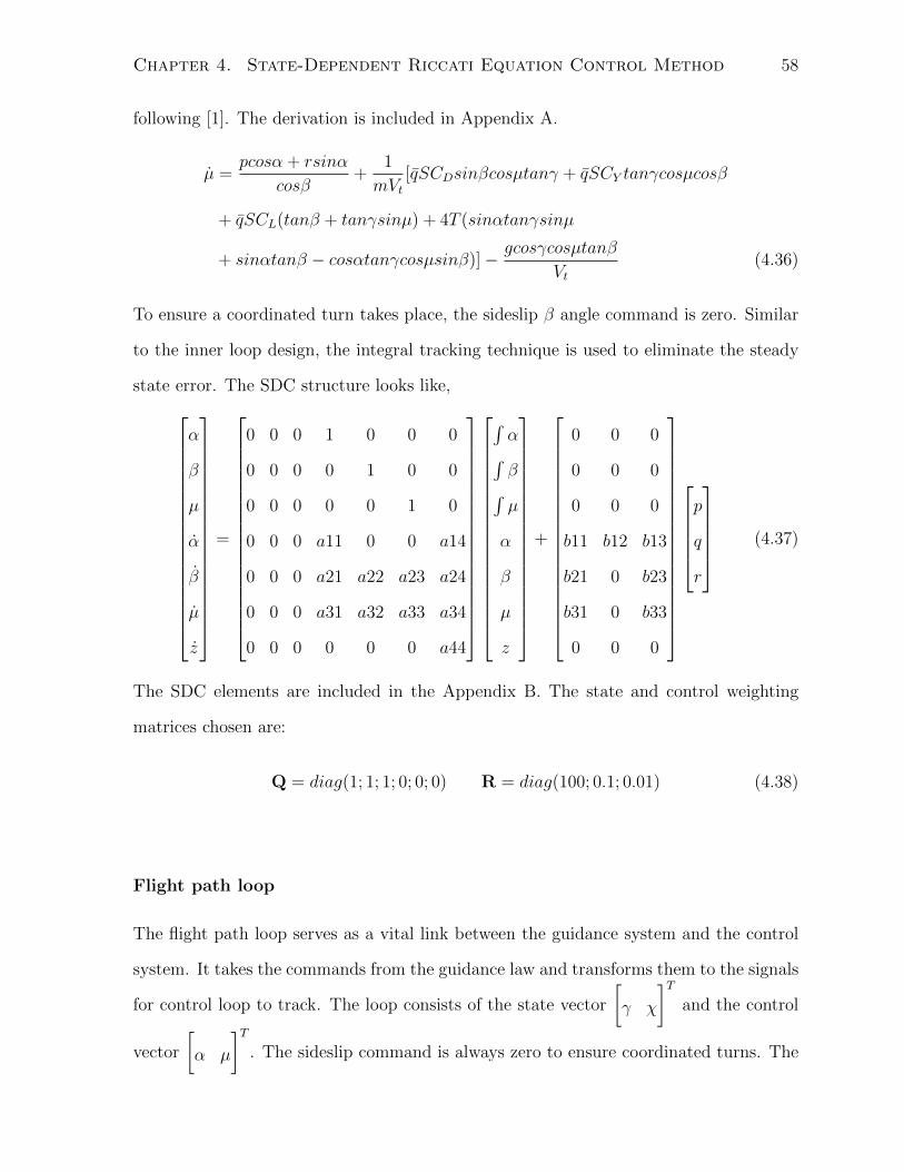
Chapter 4. State-Dependent Riccati Equation Control Method 58
following [1]. The derivation is included in Appendix A.
µ =pcosα + rsinα
cosβ+
1
mVt[qSCDsinβcosµtanγ + qSCY tanγcosµcosβ
+ qSCL(tanβ + tanγsinµ) + 4T (sinαtanγsinµ
+ sinαtanβ − cosαtanγcosµsinβ)]− gcosγcosµtanβ
Vt(4.36)
To ensure a coordinated turn takes place, the sideslip β angle command is zero. Similar
to the inner loop design, the integral tracking technique is used to eliminate the steady
state error. The SDC structure looks like,
α
β
µ
α
β
µ
z
=
0 0 0 1 0 0 0
0 0 0 0 1 0 0
0 0 0 0 0 1 0
0 0 0 a11 0 0 a14
0 0 0 a21 a22 a23 a24
0 0 0 a31 a32 a33 a34
0 0 0 0 0 0 a44
∫α∫β∫µ
α
β
µ
z
+
0 0 0
0 0 0
0 0 0
b11 b12 b13
b21 0 b23
b31 0 b33
0 0 0
p
q
r
(4.37)
The SDC elements are included in the Appendix B. The state and control weighting
matrices chosen are:
Q = diag(1; 1; 1; 0; 0; 0) R = diag(100; 0.1; 0.01) (4.38)
Flight path loop
The flight path loop serves as a vital link between the guidance system and the control
system. It takes the commands from the guidance law and transforms them to the signals
for control loop to track. The loop consists of the state vector
[γ χ
]Tand the control
vector
[α µ
]T. The sideslip command is always zero to ensure coordinated turns. The
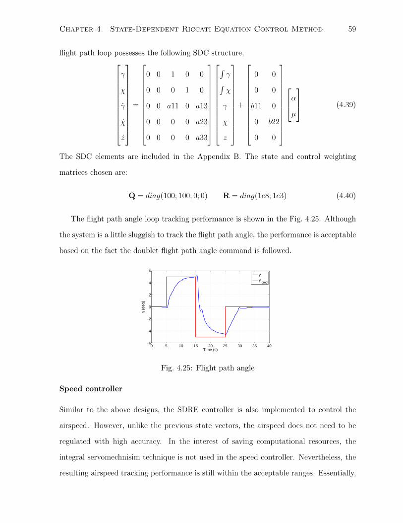
Chapter 4. State-Dependent Riccati Equation Control Method 59
flight path loop possesses the following SDC structure,
γ
χ
γ
χ
z
=
0 0 1 0 0
0 0 0 1 0
0 0 a11 0 a13
0 0 0 0 a23
0 0 0 0 a33
∫γ∫χ
γ
χ
z
+
0 0
0 0
b11 0
0 b22
0 0
αµ
(4.39)
The SDC elements are included in the Appendix B. The state and control weighting
matrices chosen are:
Q = diag(100; 100; 0; 0) R = diag(1e8; 1e3) (4.40)
The flight path angle loop tracking performance is shown in the Fig. 4.25. Although
the system is a little sluggish to track the flight path angle, the performance is acceptable
based on the fact the doublet flight path angle command is followed.
0 5 10 15 20 25 30 35 40−6
−4
−2
0
2
4
6
Time (s)
γ (d
eg)
γγ
cmd
Fig. 4.25: Flight path angle
Speed controller
Similar to the above designs, the SDRE controller is also implemented to control the
airspeed. However, unlike the previous state vectors, the airspeed does not need to be
regulated with high accuracy. In the interest of saving computational resources, the
integral servomechnisim technique is not used in the speed controller. Nevertheless, the
resulting airspeed tracking performance is still within the acceptable ranges. Essentially,
Chapter 4. State-Dependent Riccati Equation Control Method 60
this loop is the scalar case SDRE design. The state is Vt and the control is δth. The
parameterized equation is,
Vt = [−qSmVt
(CDcosα− CLsinα)cosαcosβ − g
Vtsinθcosαcosβ
+qS
mVtCY sinβ +
g
Vtcosθsinφsinβ − qS
mVt(CDsinα + CLcosα)cosβsinα
+g
Vtcosθcosφcosβsinα]Vt + (
4T
mcosαcosβ − 0.0436
4T
mcosβsinα)δth (4.41)
where T is the single engine thrust force. The state and control weighting numbers chosen
for the speed controller are:
Q = 0.1 R = 0.01 (4.42)
The control law becomes,
δth = Kth(Vt)(Vt − Vtref ) + δth0 (4.43)
where Kth(Vt) is the state-dependent control gain; Vtref is the airspeed command and δth0
is the trimmed throttle setting.
Simulation example
A landing trajectory tracking problem simulated with actuators damage is presented
here. In this problem, the aircraft descends from 3000m to the runway following a pre-
defined trajectory, based on the guidance algorithm generating the tracking commands
for the control system. During the approach, in addition to the actuator damage, the
aircraft also suffers a thrust loss of 20%. The damages are included at the begining of the
simulation. Fig. 4.26 shows the aircraft flight path angle history during the appraoch. It
is expected to follow a -4 deg. glide slope. About 250 seconds, the aircraft is transitioning
from the glide slope to flare phase. The airspeed is maintained during the appraoch as
shown by Fig. 4.28. Under the guidance and control framework, the aircraft is able
to complete the trajectory and approach the runway without incident, as illustrate in
Fig. 4.30.
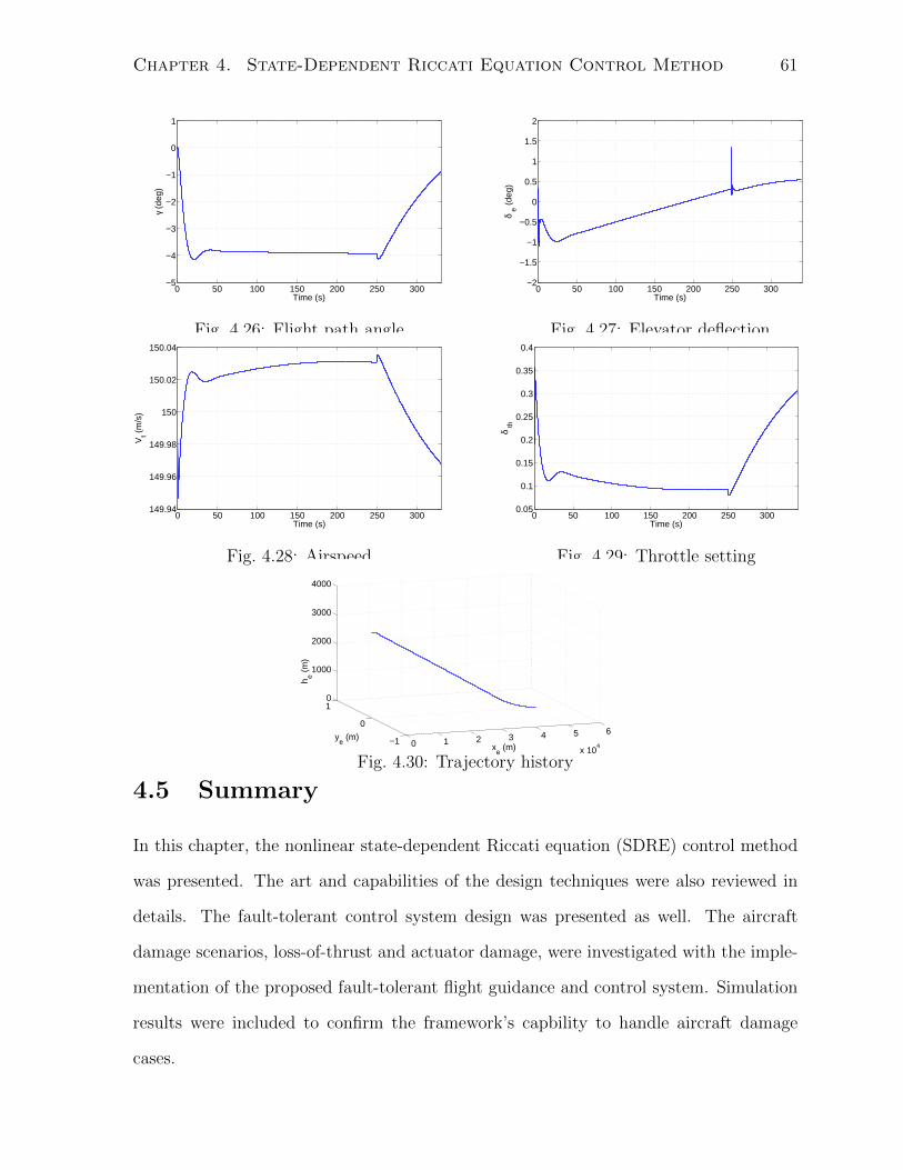
Chapter 4. State-Dependent Riccati Equation Control Method 61
0 50 100 150 200 250 300−5
−4
−3
−2
−1
0
1
Time (s)
γ (d
eg)
Fig. 4.26: Flight path angle
0 50 100 150 200 250 300−2
−1.5
−1
−0.5
0
0.5
1
1.5
2
Time (s)
δ e (
deg)
Fig. 4.27: Elevator deflection
0 50 100 150 200 250 300149.94
149.96
149.98
150
150.02
150.04
Time (s)
Vt (
m/s
)
Fig. 4.28: Airspeed
0 50 100 150 200 250 3000.05
0.1
0.15
0.2
0.25
0.3
0.35
0.4
Time (s)
δ th
Fig. 4.29: Throttle setting
0 1 2 3 4 5 6
x 104
−1
0
10
1000
2000
3000
4000
xe (m)
ye (m)
h e (m
)
Fig. 4.30: Trajectory history
4.5 Summary
In this chapter, the nonlinear state-dependent Riccati equation (SDRE) control method
was presented. The art and capabilities of the design techniques were also reviewed in
details. The fault-tolerant control system design was presented as well. The aircraft
damage scenarios, loss-of-thrust and actuator damage, were investigated with the imple-
mentation of the proposed fault-tolerant flight guidance and control system. Simulation
results were included to confirm the framework’s capbility to handle aircraft damage
cases.
Chapter 5
Adaptive State-Dependent Riccati
Equation Control Method
In this chapter, a novel nonlinear control method is proposed and implemented in the
fault-tolerant framework to evaluate its performance. The new control method is based on
the nonlinear state-dependent Riccati equation control method as the baseline controller,
but is also augmented with the model reference adaptive control method.
The research work in adaptive control started as early as the 1950’s. It was mainly
targeted at autopilot design for high performance aircraft. However, the tragic test flight
of X-15 diminished the interest in adaptive control from the community at that time. In
recent years, there has been increasing development of a coherent theory and practical
application of adaptive control, which has tremendous potential for the flight control com-
munity. Adaptive control deals with complex systems that have unpredictable parameter
derivations and uncertainties. Unlike robust control, which has the advantage of dealing
with disturbances, fast varying parameters, and unmodeled dynamics, adaptive control
is superior for handling uncertainties in constants or slowly varying parameters. When
the aircraft suffers from damage, the initial dynamics change can be sudden and drastic.
However the subsequent dynamics change will be slow once the aircraft is stabilized by
the control system. The aerodynamic coefficients variations are the main factors to the
62
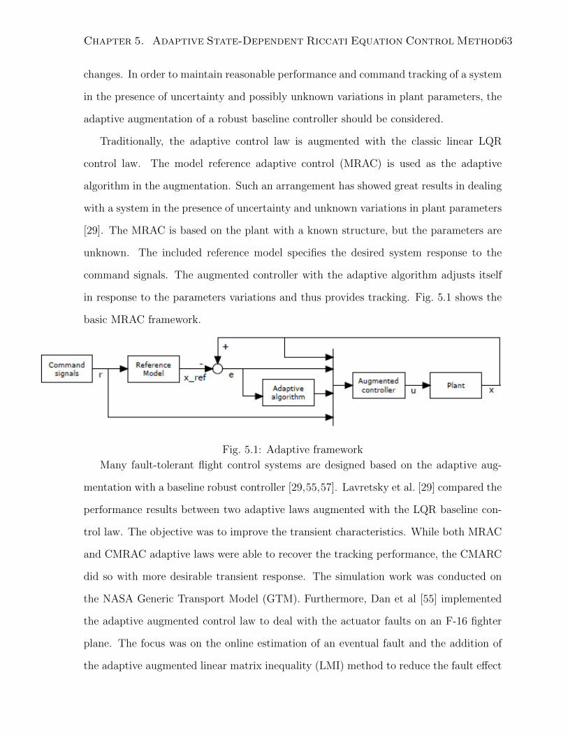
Chapter 5. Adaptive State-Dependent Riccati Equation Control Method63
changes. In order to maintain reasonable performance and command tracking of a system
in the presence of uncertainty and possibly unknown variations in plant parameters, the
adaptive augmentation of a robust baseline controller should be considered.
Traditionally, the adaptive control law is augmented with the classic linear LQR
control law. The model reference adaptive control (MRAC) is used as the adaptive
algorithm in the augmentation. Such an arrangement has showed great results in dealing
with a system in the presence of uncertainty and unknown variations in plant parameters
[29]. The MRAC is based on the plant with a known structure, but the parameters are
unknown. The included reference model specifies the desired system response to the
command signals. The augmented controller with the adaptive algorithm adjusts itself
in response to the parameters variations and thus provides tracking. Fig. 5.1 shows the
basic MRAC framework.
Fig. 5.1: Adaptive framework
Many fault-tolerant flight control systems are designed based on the adaptive aug-
mentation with a baseline robust controller [29,55,57]. Lavretsky et al. [29] compared the
performance results between two adaptive laws augmented with the LQR baseline con-
trol law. The objective was to improve the transient characteristics. While both MRAC
and CMRAC adaptive laws were able to recover the tracking performance, the CMARC
did so with more desirable transient response. The simulation work was conducted on
the NASA Generic Transport Model (GTM). Furthermore, Dan et al [55] implemented
the adaptive augmented control law to deal with the actuator faults on an F-16 fighter
plane. The focus was on the online estimation of an eventual fault and the addition of
the adaptive augmented linear matrix inequality (LMI) method to reduce the fault effect
Chapter 5. Adaptive State-Dependent Riccati Equation Control Method64
on the system without the need for a fault detection and isolation mechanism.
Although the linear control method is most often the choice when augmenting with
the adaptive law, the augmented system still needs gain scheduling to accommodate the
entire flight envelop. This procedure further complicates the already complex design
process. On the other hand, the advantages of nonlinear control method is that it offers
much more flexibility than its counterpart when dealing with augmentation. For example,
Lombaerts et al. [30] proposed a sophisticated flight control law based on nonlinear
dynamic inversion. It is well known that the dynamic inversion method is prone to
erroneous inversion due to model mismatch and uncertainties in the parameters. To
overcome the problem, a two-step algorithm was developed to estimate the parameters
online and adapt the parameter variations. The algorithm was implemented on the
SIMONA Research Simulator [30].
The proposed adaptive augmented control is based on the SDRE control method
and MRAC. The proposed framework has many advantages over the existing linear one.
First of all, the baseline SDRE method is a very effective and systematic control method.
Unlike many other nonlinear methods, it is based on a systematic design process. In other
words, the method can be readily implemented to different kinds of nonlinear systems.
Secondly, as demonstrated in the previous chapter, the SDRE method is able to deal
with complicated and difficult control problems involved with non-affine in control, state
and control constraints. These features are especially important in the context of fault-
tolerant flight control. Additionally, being a robust nonlinear control method itself, it has
the advantage of actively updating the feedback gain at each step to accommodate the
parameter changes. In a way, it also adapts itself to the varying environment. Finally,
using the SDRE as the baseline controller avoids the complex gain scheduling process in
the flight control system.
In the next section, the augmented control method is formally introduced. The math-
ematical formulation and problem definition are presented. Subsequently, the stability
Chapter 5. Adaptive State-Dependent Riccati Equation Control Method65
analysis is included for the proposed controller to show its viability. Finally, the novel con-
trol method is implemented on the NASA GTM simulink model to test its performance.
Comparisons are also made in Section 5.3 to investigate the controller’s performance.
5.1 Adaptive Control Method
In this section, the novel adaptive state-dependent Riccai equation control method is
introduced. It is based on the nonlinear state-dependent Riccati equation control method
and the model reference adaptive control law. The augmentation aims to provide superior
tracking performance and transient response than its baseline controller.
Consider the general autonomous, affine-in-control, nonlinear system dynamics in the
form of,
x = f(x) + B(x)u(t) x(0) = x0 (5.1)
where the state vector x ∈ <n, and the control vectoru ∈ <m. Assume the dynamics
satisfy the SDRE conditions stated earlier, so the system can be expressed with state
dependent coefficients.
xp = Ap(xp)xp + Bp(xp)u (5.2)
where f = Ap(xp)xp. The control goal is to ensure bounded tracking. The system
controlled output,
y(x) = Cp(xp)xp ∈ <m (5.3)
tracks any bounded and possibly time-varying command signal r(t) ∈ <m with bounded
errors in the presence of the system uncertainties. Let
e(t) = y(t)− r(t) (5.4)
denote the system output tracking error. The system uncertainties can be reflected in
the state dependent coefficients. In the case of damage, A(x) and B(x) vary in terms of
Chapter 5. Adaptive State-Dependent Riccati Equation Control Method66
their individual elements. As a result, new state-dependent matrices can be defined as,
A(x) = Ap(xp)−∆A(x) (5.5)
B(x) = Bp(xp)−∆B(x) (5.6)
Consider that
x = xp −∆x (5.7)
Taking the derivative of Eq.5.7 and Substitute Eq.(5.5) and (5.6) into Eq.(5.2),
x = A(x)x + B(x)u + [∆A(x)x + ∆B(x)u] (5.8)
where the δx contribution is small enough to be neglected when multiplied by state-
dependent matrix A(x). The time derivative of δx is assumed to zero. Eq.(5.8) represents
the expanded system dynamics including the uncertainties. It is also reasonable to assume
that the last two terms of Eq.5.8 are much less than the first two terms. As a result,
x = A(x)x+ B(x) (5.9)
Model reference adaptive control is based on the assumption of model matching. It as-
sumes that given a reference Hurwitz matrix Aref , there must exist, a possibly unknown,
gain matrix Kx such that,
Aref (x) = A(x) + B(x)KTx (5.10)
Substitute Eq.(5.10) into Eq.(5.8) and rearranging the terms with the relationships of
Eq.(5.5) and Eq.(5.6),
x = Aref (x)x + [−(B(x)KTx x + B(x)u] (5.11)
As a result,
u(x) = KTx (x)x (5.12)
where Kx(x) ∈ <n×m is the adaptive gain matrix, whose dynamics will be defined later.
Chapter 5. Adaptive State-Dependent Riccati Equation Control Method67
The reference model dynamics are,
xref = Aref (xref )xref (5.13)
Let the system tracking error be,
e(x) = x− xref (5.14)
Note the tracking error is also state dependent. Its value varies at the each step. The
tracking error dynamics can be obtained by subtracting the reference state dynamics
from the system dynamics as,
e(x) = Aref (x)e(x) + B(x)(KTx (x)−KT
x (x))x (5.15)
The objective is to design state-dependent feedback gain Kx such that the track-
ing error goes to zero. The direct model reference adaptive control law and Lyapunov
arguments can be used as shown in the next section to derive the control law,
˙Kx = −Γxxe(x)TPref (x)B(x) (5.16)
where Pref (x) = P Tref (x) > 0 is the unique symmetric, state-dependent, positive definite
solution to the state-dependent algebraic Lyapunov equation,
ATref (x)Pref (x) + Pref (x)Aref (x) = −Qref (x) (5.17)
where Qref (x) = QTref (x) > 0 is similar to the state-dependent weighting matrix Q(x)
in the ARE. Using the state-dependent feedback gain in Eq.(5.16) and the relation in
Eq.(5.17), one can solve the above stated tracking problem with asymptotically stable
closed-loop dynamics. The in-depth stability analysis is presented in the next section.
Similar to the standard direct model reference adaptive control laws, the solution is valid
for any symmetric positive definite rates of adaptation Γx. As later demonstrated in the
example, the adaptation rate cannot be arbitrarily large, or unwanted oscillation and
unnecessary computational burden will occur.
Chapter 5. Adaptive State-Dependent Riccati Equation Control Method68
5.2 Stability Studies
In this section, the stability analysis of the proposed state-dependent adaptive control
method is offered. It is important to note that the baseline controller of this novel
augmented control method is the nonlinear SDRE method. As proven in the previous
chapter, the SDRE control method is locally asymptotically stable and is only glob-
ally stable in special cases. Since the underlying controller is only locally stable, the
augmented control method is proved to be locally stable in this section. However, the
necessary global asymptotic stable condition will be given at the end of the analysis.
5.2.1 Stability Analysis
To prove the augmented control method is locally stable, a suitable Lyapunov function
candidate is chosen,
V (e,∆Kx) = eT(x)Pref (x)e(x) + trace(∆KTx Γ−1x ∆KxΓ) (5.18)
where Γx = ΓTx > 0 denotes the rate of adaptation. PTref (x) = Pref (x) > 0 is the state
dependent solution to the state dependent algebraic Lyapunov equation Eq.(5.17). The
stability analysis is mainly based on the following theorem,
Theorem 5. [27] Let x = 0 be an equilibrium point for Eq.(5.1) and D ⊂ <n be a
domain containing x = 0. Let V : [0,∞) × D 7→ < be a continuously differentiable
function such that
W1(x) ≤ V (t, x) ≤ W2(x) (5.19)
∂V
∂t+∂V
∂xf(t, x) ≤ −W3(x) (5.20)
∀t ≥ 0, ∀x ∈ D where W1(x), W2(x), and W3(x) are continuous positive definite functions
on D. Then, x = 0 is uniformly asymptotically stable.
Chapter 5. Adaptive State-Dependent Riccati Equation Control Method69
Taking the time derivative of the Lyapunov function evaluated along the error dy-
namics trajectory gives,
V (x) =∂V
∂t+∂V
∂xf(t, x) (5.21)
=∂V
∂xf(t, x) (5.22)
where ∂V∂t
= 0 Based on Theorem 5, the following new theorem is established for the
proposed control method.
Theorem 6. Given a Lyapunov function candidate, if the function satisfies the conditions
in Theorem 5, then the closed loop system under the state-dependent adaptive feedback
control is locally asymptotically stable.
Proof. The derivative of the Lyapunov function becomes,
V (x) = e(x)Pref (x)e(x)+eT(x)Pref (x)e(x)+eT(x)Pref (x)e(x)+2trace(∆KTx Γ−1 ˙Kx)
(5.23)
Substitute the error dynamics as well as the Riccati differential equation into this,
P(x) = −AT(x)P(x)−P(x)A(x) + P(x)B(x)BT(x)P(x)−Q(x) (5.24)
However, the Lyapunov inequality is more appropriate in this case,
P(x) + AT(x)P(x) + P(x)A(x) + Q(x) ≤ 0 (5.25)
So the derivative of the Lyapunov function becomes,
V (x) ≤ [Aref (x)e(x) + B(x)(KTx (x)−KT
x (x))x]TPref (x)e(x) (5.26)
+ eT(x)[−ATref (x)Pref (x)−Pref (x)Aref (x)−Qref (x)]e(x) (5.27)
+ 2trace(∆KTx Γ−1 ˙Kx) (5.28)
Rearranging terms,
V (x) ≤ −eT(x)Qrefe(x) + 2eT(x)Pref (x)B(x)∆KTx x (5.29)
+ 2trace(∆KTx Γ−1 ˙Kx) (5.30)
Chapter 5. Adaptive State-Dependent Riccati Equation Control Method70
Define the training error signal as
e(x) = BT(x)Pref (x)e(x) (5.31)
and applying the trace identity the Lyapunov function derivative becomes,
V (x) ≤ −eT(x)Qrefe(x) + 2trace(∆KTx xeT(x)) + 2trace(∆KT
x Γ−1 ˙Kx) (5.32)
and collecting and rearranging terms
V (x) ≤ −eT(x)Qrefe(x) + 2trace[∆KTx (Γ−1Kx + xeT)] (5.33)
and choosing the control gain to be,
˙Kx = −ΓxeT(x)Pref (x)B(x) (5.34)
implies that
V ≤ 0 (5.35)
Eq.(5.35) confirms the Lyapunov function satisfies the second condition, Eq.(5.20), in
Theorem 5. In other words, W3(x) = 0 in our case. The first condition can be satisfied
automatically given the fact that both W1(x) and W2(x) can be set to V (x) at each
step to ensure the condition. As a result, Theorem 5 is satisfied. However, one must
remember that the augmented controller relies on the baseline SDRE controller to provide
the Aref (x). As proved earlier in the Chapter, SDRE is locally stable. Thus, Aref (x) can
only be a local Hurwitz matrix. Thus, the augmented controller is locally asymptotically
stable.
As mentioned earlier, the global stable property of the augmented adaptive control
method is possible under special circumstances dictated by the SDRE control method.
The necessary condition to guarantee the global stable property is given here.
Corollary 1. The SDRE and MRAC augmented control method is globally stable if the
following conditions are met:
Chapter 5. Adaptive State-Dependent Riccati Equation Control Method71
• SDRE controller is proven to be globally asymptotically stable
• Theorem 5 is satisfied
Proof. When the SDRE controller is globally asymptotically stable, it implies thatAref (x)
is always a Hurwitz matrix. As a result, the Theorem 6 derivation result V ≤ 0 is valid
in the global sense given the conditions of Theorem 5 are satisfied.
5.3 Simulation Studies
In this section, the proposed state-dependent adaptive control method is implemented
on the NASA GTM model to study its performance with airframe damage. The method
is also compared with the regular SDRE control method to investigate the performance
enhancement.
The damage scenario is provided by the GTM simulink model as damage case six,
see Sec. 2.4. The entire left stabilizer suffers damage, and this results the elimination of
the left elevator. A more detailed damage case description was presented in Chapter 2.
The nonlinear controller design for the GTM is particularly a difficult task. The
aircraft nonlinear dynamics equations are slightly different from the traditional flight
dynamics due to the offset between the center of pressure and center of mass. Secondly,
the nonlinear aerodynamic coefficients are complex. They require translation from the
simulink model to the analytic forms to fit the control design. Furthermore, similar
to the B747 design case, the system is also non-affine in control due to the nonlinear
characteristics of the aerodynamic coefficients.
α =1
mVtcosβ(−Fxsinα + Fzcos(α) +mVt(−pcosαsinβ + qcosβ − rsinαsinβ)) (5.36)
q = c5pr − c6(p2 − r2) + c7My (5.37)
To demonstrate the novel control method, the NASA GTM model short period dynamics
are considered. The following equations are the same ones identified in Chapter 2. The
Chapter 5. Adaptive State-Dependent Riccati Equation Control Method72
forces and moment equations are,
Fx = qS(CXbasic + CXdynamic + CXcontrol) + Fxcontrol + Fxgravity (5.38)
Fz = qS(CXbasic + CXdynamic + CXcontrol) + Fzcontrol + Fzgravity (5.39)
My = qSc(Cmbasic + Cmdynamic) + rz qS(CXbasic + CXdynamic)
− rxqS(CZbasic + CZdynamic) +Myengine + qScCmcontrol + rz qSCXcontrol
− rxqSCZcontrol (5.40)
where rx = cpx − cgx and rz = cpz − cgz are the cp and cg offsets in x and z axes.
Similar to the B747 longitudinal case, Fx, Fy, and My represent the aerodynamic forces
and moments. In the forces case, the contributions include the aerodynamic coefficients,
(such as CXbaic , CXdynamic , CXcontrol), control terms (such as Fxcontrol), and the gravity
force terms (such as Fxgravity). These terms can all be expressed by a series of stability
derivatives that are included in the simulink model as look-up tables. In the case of the
moment, because of the difference between the cp and the cg, the aerodynamic forces
also contribute in the equation.
5.3.1 Baseline Control
The baseline control design is presented in this section. The first step is to parameterize
the above dynamics into the state-dependent coefficients form. The original dynamics
include bias terms. It means that a slow state z needs to be introduced to deal with the
issue.
x =
0 a12 a13
0 0 a23
0 0 a31
α
q
z
+
b11
b12
0
δe (5.41)
The SDC elements are included in Appendix B. The NASA GTM model is trimmed
to 3 deg. angle of attack, straight and level flight. In this example, the angle of attack
is selected to be the tracking signal. The integral servomechanism is formulated to
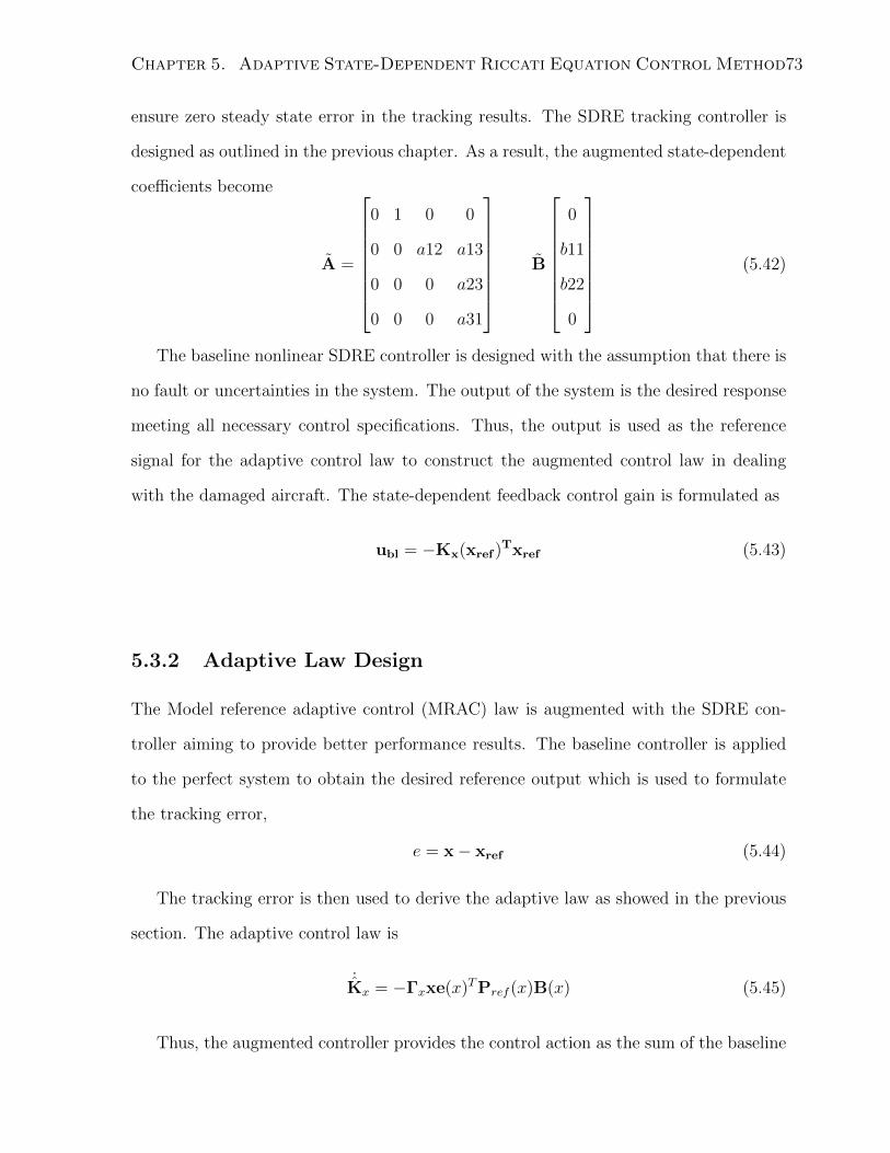
Chapter 5. Adaptive State-Dependent Riccati Equation Control Method73
ensure zero steady state error in the tracking results. The SDRE tracking controller is
designed as outlined in the previous chapter. As a result, the augmented state-dependent
coefficients become
A =
0 1 0 0
0 0 a12 a13
0 0 0 a23
0 0 0 a31
B
0
b11
b22
0
(5.42)
The baseline nonlinear SDRE controller is designed with the assumption that there is
no fault or uncertainties in the system. The output of the system is the desired response
meeting all necessary control specifications. Thus, the output is used as the reference
signal for the adaptive control law to construct the augmented control law in dealing
with the damaged aircraft. The state-dependent feedback control gain is formulated as
ubl = −Kx(xref )Txref (5.43)
5.3.2 Adaptive Law Design
The Model reference adaptive control (MRAC) law is augmented with the SDRE con-
troller aiming to provide better performance results. The baseline controller is applied
to the perfect system to obtain the desired reference output which is used to formulate
the tracking error,
e = x− xref (5.44)
The tracking error is then used to derive the adaptive law as showed in the previous
section. The adaptive control law is
˙Kx = −Γxxe(x)TPref (x)B(x) (5.45)
Thus, the augmented controller provides the control action as the sum of the baseline
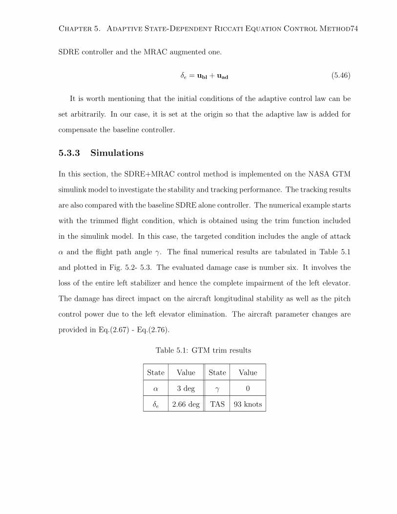
Chapter 5. Adaptive State-Dependent Riccati Equation Control Method74
SDRE controller and the MRAC augmented one.
δe = ubl + uad (5.46)
It is worth mentioning that the initial conditions of the adaptive control law can be
set arbitrarily. In our case, it is set at the origin so that the adaptive law is added for
compensate the baseline controller.
5.3.3 Simulations
In this section, the SDRE+MRAC control method is implemented on the NASA GTM
simulink model to investigate the stability and tracking performance. The tracking results
are also compared with the baseline SDRE alone controller. The numerical example starts
with the trimmed flight condition, which is obtained using the trim function included
in the simulink model. In this case, the targeted condition includes the angle of attack
α and the flight path angle γ. The final numerical results are tabulated in Table 5.1
and plotted in Fig. 5.2- 5.3. The evaluated damage case is number six. It involves the
loss of the entire left stabilizer and hence the complete impairment of the left elevator.
The damage has direct impact on the aircraft longitudinal stability as well as the pitch
control power due to the left elevator elimination. The aircraft parameter changes are
provided in Eq.(2.67) - Eq.(2.76).
Table 5.1: GTM trim results
State Value State Value
α 3 deg γ 0
δe 2.66 deg TAS 93 knots
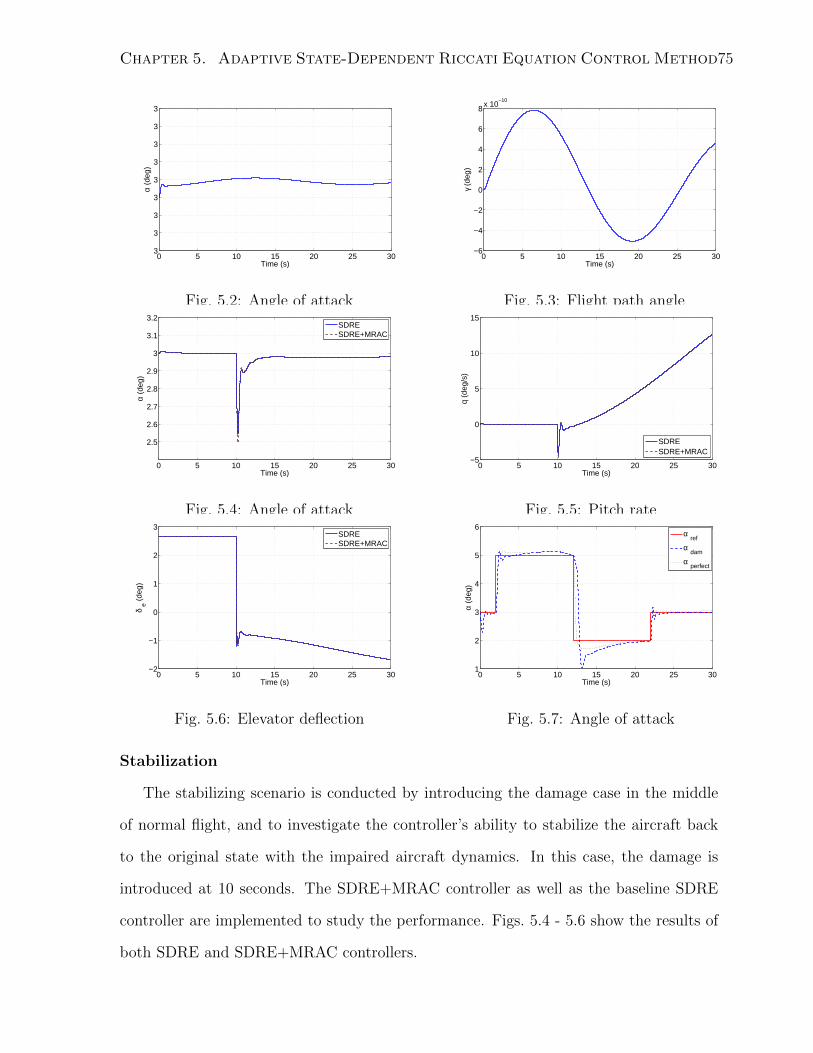
Chapter 5. Adaptive State-Dependent Riccati Equation Control Method75
0 5 10 15 20 25 303
3
3
3
3
3
3
3
3
Time (s)
α (d
eg)
Fig. 5.2: Angle of attack
0 5 10 15 20 25 30−6
−4
−2
0
2
4
6
8x 10
−10
Time (s)
γ (d
eg)
Fig. 5.3: Flight path angle
0 5 10 15 20 25 30
2.5
2.6
2.7
2.8
2.9
3
3.1
3.2
Time (s)
α (d
eg)
SDRESDRE+MRAC
Fig. 5.4: Angle of attack
0 5 10 15 20 25 30−5
0
5
10
15
Time (s)q
(deg
/s)
SDRESDRE+MRAC
Fig. 5.5: Pitch rate
0 5 10 15 20 25 30−2
−1
0
1
2
3
Time (s)
δ e (
deg)
SDRESDRE+MRAC
Fig. 5.6: Elevator deflection
0 5 10 15 20 25 301
2
3
4
5
6
Time (s)
α (d
eg)
α ref
α dam
α perfect
Fig. 5.7: Angle of attack
Stabilization
The stabilizing scenario is conducted by introducing the damage case in the middle
of normal flight, and to investigate the controller’s ability to stabilize the aircraft back
to the original state with the impaired aircraft dynamics. In this case, the damage is
introduced at 10 seconds. The SDRE+MRAC controller as well as the baseline SDRE
controller are implemented to study the performance. Figs. 5.4 - 5.6 show the results of
both SDRE and SDRE+MRAC controllers.
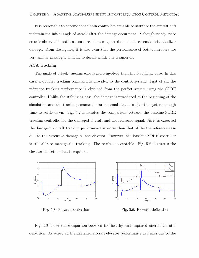
Chapter 5. Adaptive State-Dependent Riccati Equation Control Method76
It is reasonable to conclude that both controllers are able to stabilize the aircraft and
maintain the initial angle of attack after the damage occurrence. Although steady state
error is observed in both case such results are expected due to the extensive left stabilizer
damage. From the figures, it is also clear that the performance of both controllers are
very similar making it difficult to decide which one is superior.
AOA tracking
The angle of attack tracking case is more involved than the stabilizing case. In this
case, a doublet tracking command is provided to the control system. First of all, the
reference tracking performance is obtained from the perfect system using the SDRE
controller. Unlike the stabilizing case, the damage is introduced at the beginning of the
simulation and the tracking command starts seconds later to give the system enough
time to settle down. Fig. 5.7 illustrates the comparison between the baseline SDRE
tracking controller for the damaged aircraft and the reference signal. As it is expected
the damaged aircraft tracking performance is worse than that of the the reference case
due to the extensive damage to the elevator. However, the baseline SDRE controller
is still able to manage the tracking. The result is acceptable. Fig. 5.8 illustrates the
elevator deflection that is required.
0 5 10 15 20 25 300
1
2
3
4
5
6
Time (s)
δ e (
deg)
Fig. 5.8: Elevator deflection
0 5 10 15 20 25 30−4
−2
0
2
4
6
Time (s)
δ e (
deg)
δ e
dam
δe
perfect
Fig. 5.9: Elevator deflection
Fig. 5.9 shows the comparison between the healthy and impaired aircraft elevator
deflection. As expected the damaged aircraft elevator performance degrades due to the
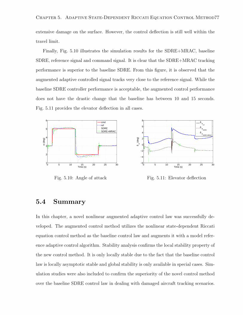
Chapter 5. Adaptive State-Dependent Riccati Equation Control Method77
extensive damage on the surface. However, the control deflection is still well within the
travel limit.
Finally, Fig. 5.10 illustrates the simulation results for the SDRE+MRAC, baseline
SDRE, reference signal and command signal. It is clear that the SDRE+MRAC tracking
performance is superior to the baseline SDRE. From this figure, it is observed that the
augmented adaptive controlled signal tracks very close to the reference signal. While the
baseline SDRE controller performance is acceptable, the augmented control performance
does not have the drastic change that the baseline has between 10 and 15 seconds.
Fig. 5.11 provides the elevator deflection in all cases.
0 5 10 15 20 25 301
2
3
4
5
6
Time (s)
α (d
eg)
cmdrefSDRESDRE+MRAC
Fig. 5.10: Angle of attack
0 5 10 15 20 25 30−6
−4
−2
0
2
4
6
8
Time (s)
δ e (
deg)
δ e
ref
δ e
SDRE
δ e
SDRE+MRAC
Fig. 5.11: Elevator deflection
5.4 Summary
In this chapter, a novel nonlinear augmented adaptive control law was successfully de-
veloped. The augmented control method utilizes the nonlinear state-dependent Riccati
equation control method as the baseline control law and augments it with a model refer-
ence adaptive control algorithm. Stability analysis confirms the local stability property of
the new control method. It is only locally stable due to the fact that the baseline control
law is locally asymptotic stable and global stability is only available in special cases. Sim-
ulation studies were also included to confirm the superiority of the novel control method
over the baseline SDRE control law in dealing with damaged aircraft tracking scenarios.
Chapter 6
Conclusions and Future Work
The objective of this thesis was to investigate and develop a nonlinear fault-tolerant flight
control design to deal with aircraft that suffer from the various degrees of damage, such as
loss of thrust, actuator malfunction and/or airframe damage. A design framework was
developed to accommodate the damaged aircraft while achieving close to the original
system performance.
The proposed design framework includes a guidance law and a control law to deal
with damaged aircraft. The guidance law was based on the zero-effort miss concept
to provide the flight path commands to the control system while taking into account
the impaired aircraft dynamics. The SDRE control method was used to design the
fault-tolerant flight control laws. The nonlinear SDRE control method demonstrated its
passive adaptive features and robust performance in the simulation studies. In order
to ensure the aircraft parameter variations due to damage were properly considered, a
novel nonlinear adaptive control law based on SDRE was proposed in this research. The
method demonstrated improved tracking performance and the potential to be considered
as an adaptive fault-tolerant flight control method. The proposed framework was applied
to nonlinear B747 and NASA GTM aircraft models to demonstrate its capability.
Future research will focus on the modeling and simulation of more sophisticated and
78
Chapter 6. Conclusions and Future Work 79
realistic aircraft damage scenarios. The simulation model fidelity is an important issue.
In order to obtain realistic simulation results, the aircraft simulation model should include
more relevant stability derivatives. This issue can be dealt with using two approaches.
The first one requires access to flight test data. Using actual flight test data to evaluate
the control method is the desired approach for future work. The second approach is to
analytically derive modified equations of motion that include damage effects so that the
complex coupling can be taken into account as part of the design process. In addition,
while the fault-tolerant flight control system provides promising results in terms of dealing
with in-flight aircraft damage, the current research work is only a preliminary, early
stage of work, which limits its actual application to the aircraft control system design
and application. Applying the fault-tolerant flight control systems to deal with damaged
aircraft will compliment the existing aircraft control system, alleviate the pilots workload
during this critical time and increase flying safety. Thus, working towards the verification
and validation of the fault-tolerant flight control is a desirable goal.
Appendix A
Derivations
In this section, the derivations of Vt, α, and β are provided.
Airspeed dynamics
It is known that the velocity components are equal tou
v
w
= Vt
cosα · cosβ
sinβ
sinα · cosβ
(A.1)
where,
Vt =√u2 + v2 + w2 (A.2)
α = arctan(w
u) (A.3)
β = arctan(v√
u2 + w2) (A.4)
Taking the time derivative of eq.(A.2),
Vt =uu+ vv + ww
Vt(A.5)
Substituting eq.(A.1) into eq.(A.5),
Vt = ucosαcosβ + vsinβ + wsinαcosβ (A.6)
Substituting u, v, and w from the force equations, and canceling out the roll, pitch and yaw rate terms
Vt =1
m(Fxcosαcosβ + Fysinβ + Fzcosβsinα) (A.7)
80
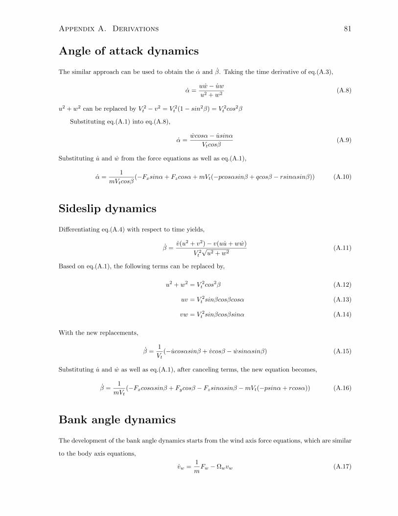
Appendix A. Derivations 81
Angle of attack dynamics
The similar approach can be used to obtain the α and β. Taking the time derivative of eq.(A.3),
α =uw − uwu2 + w2
(A.8)
u2 + w2 can be replaced by V 2t − v2 = V 2
t (1− sin2β) = V 2t cos
2β
Substituting eq.(A.1) into eq.(A.8),
α =wcosα− usinα
Vtcosβ(A.9)
Substituting u and w from the force equations as well as eq.(A.1),
α =1
mVtcosβ(−Fxsinα+ Fzcosα+mVt(−pcosαsinβ + qcosβ − rsinαsinβ)) (A.10)
Sideslip dynamics
Differentiating eq.(A.4) with respect to time yields,
β =v(u2 + v2)− v(uu+ ww)
V 2t
√u2 + w2
(A.11)
Based on eq.(A.1), the following terms can be replaced by,
u2 + w2 = V 2t cos
2β (A.12)
uv = V 2t sinβcosβcosα (A.13)
vw = V 2t sinβcosβsinα (A.14)
With the new replacements,
β =1
Vt(−ucosαsinβ + vcosβ − wsinαsinβ) (A.15)
Substituting u and w as well as eq.(A.1), after canceling terms, the new equation becomes,
β =1
mVt(−Fxcosαsinβ + Fycosβ − Fzsinαsinβ −mVt(−psinα+ rcosα)) (A.16)
Bank angle dynamics
The development of the bank angle dynamics starts from the wind axis force equations, which are similar
to the body axis equations,
vw =1
mFw − Ωwvw (A.17)
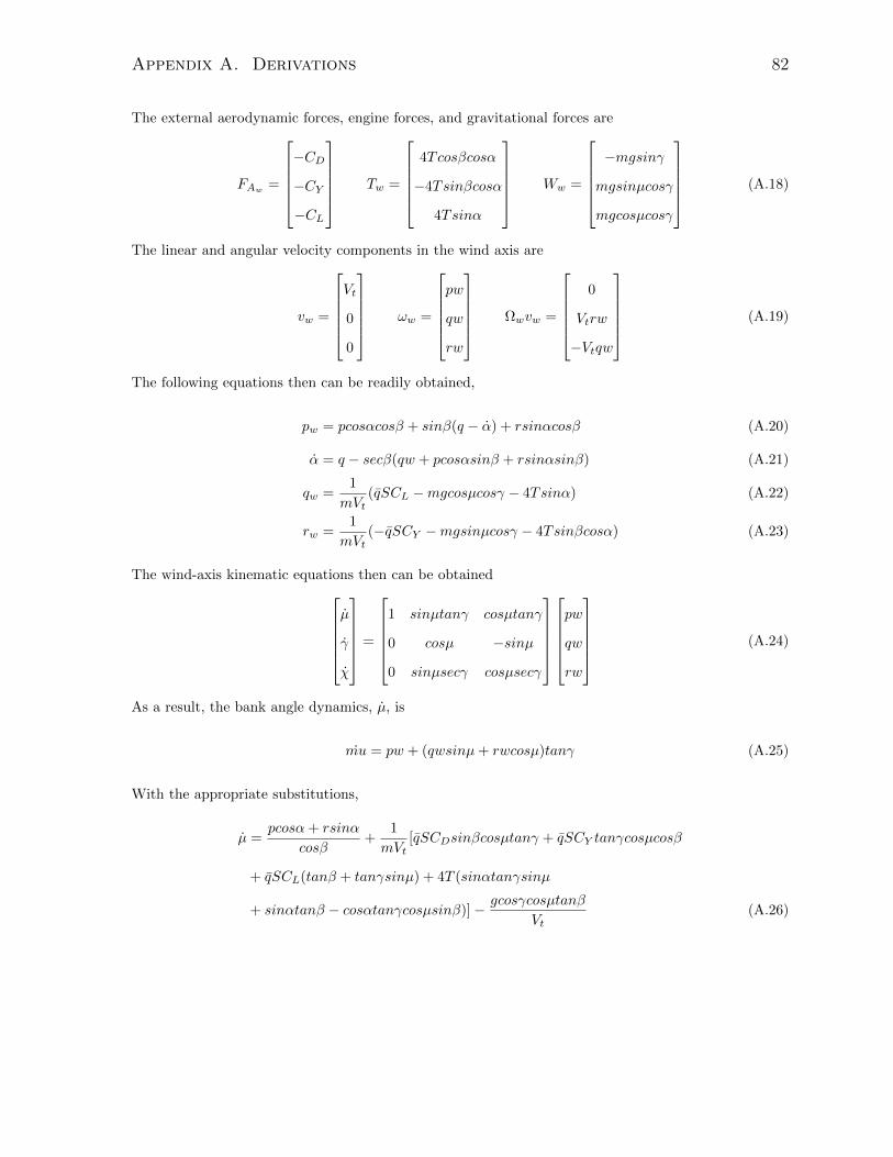
Appendix A. Derivations 82
The external aerodynamic forces, engine forces, and gravitational forces are
FAw =
−CD
−CY
−CL
Tw =
4Tcosβcosα
−4Tsinβcosα
4Tsinα
Ww =
−mgsinγ
mgsinµcosγ
mgcosµcosγ
(A.18)
The linear and angular velocity components in the wind axis are
vw =
Vt
0
0
ωw =
pw
qw
rw
Ωwvw =
0
Vtrw
−Vtqw
(A.19)
The following equations then can be readily obtained,
pw = pcosαcosβ + sinβ(q − α) + rsinαcosβ (A.20)
α = q − secβ(qw + pcosαsinβ + rsinαsinβ) (A.21)
qw =1
mVt(qSCL −mgcosµcosγ − 4Tsinα) (A.22)
rw =1
mVt(−qSCY −mgsinµcosγ − 4Tsinβcosα) (A.23)
The wind-axis kinematic equations then can be obtainedµ
γ
χ
=
1 sinµtanγ cosµtanγ
0 cosµ −sinµ
0 sinµsecγ cosµsecγ
pw
qw
rw
(A.24)
As a result, the bank angle dynamics, µ, is
mu = pw + (qwsinµ+ rwcosµ)tanγ (A.25)
With the appropriate substitutions,
µ =pcosα+ rsinα
cosβ+
1
mVt[qSCDsinβcosµtanγ + qSCY tanγcosµcosβ
+ qSCL(tanβ + tanγsinµ) + 4T (sinαtanγsinµ
+ sinαtanβ − cosαtanγcosµsinβ)]− gcosγcosµtanβ
Vt(A.26)
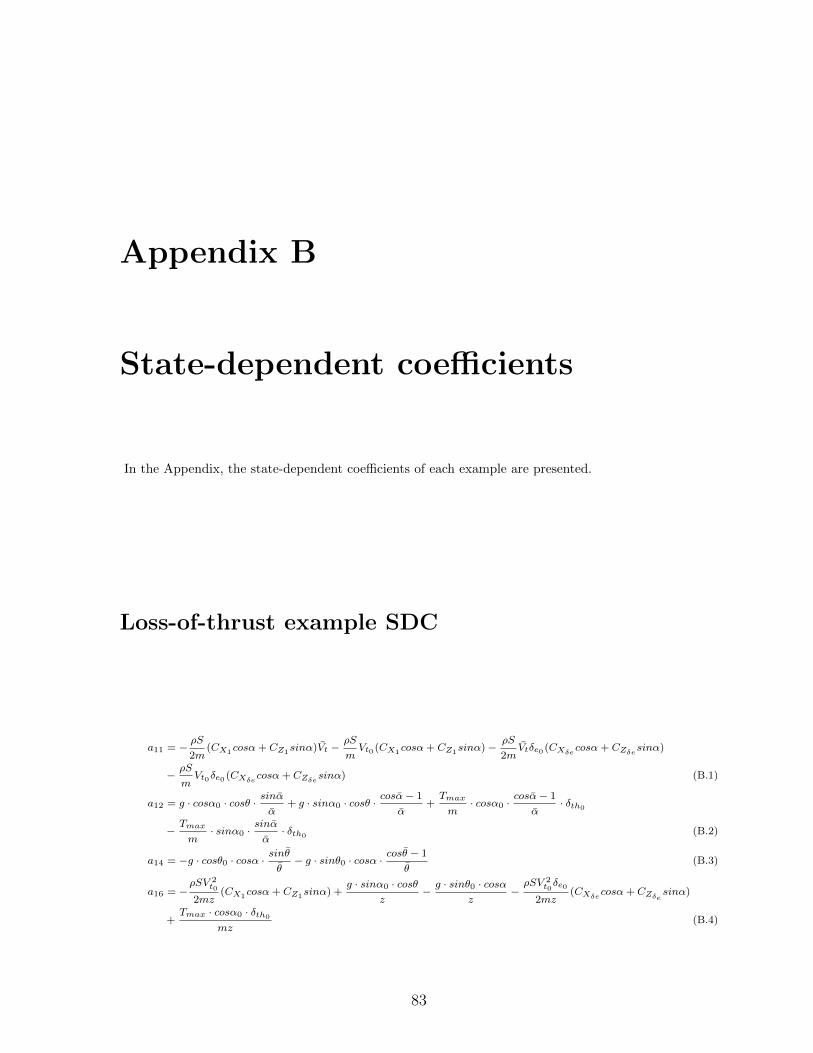
Appendix B
State-dependent coefficients
In the Appendix, the state-dependent coefficients of each example are presented.
Loss-of-thrust example SDC
a11 = −ρS
2m(CX1cosα+ CZ1sinα)Vt −
ρS
mVt0 (CX1cosα+ CZ1sinα)−
ρS
2mVtδe0 (CXδecosα+ CZδesinα)
−ρS
mVt0δe0 (CXδecosα+ CZδesinα) (B.1)
a12 = g · cosα0 · cosθ ·sinα
α+ g · sinα0 · cosθ ·
cosα− 1
α+Tmax
m· cosα0 ·
cosα− 1
α· δth0
−Tmax
m· sinα0 ·
sinα
α· δth0
(B.2)
a14 = −g · cosθ0 · cosα ·sinθ
θ− g · sinθ0 · cosα ·
cosθ − 1
θ(B.3)
a16 = −ρSV 2
t0
2mz(CX1
cosα+ CZ1sinα) +
g · sinα0 · cosθz
−g · sinθ0 · cosα
z−ρSV 2
t0δe0
2mz(CXδecosα+ CZδe sinα)
+Tmax · cosα0 · δth0
mz(B.4)
83
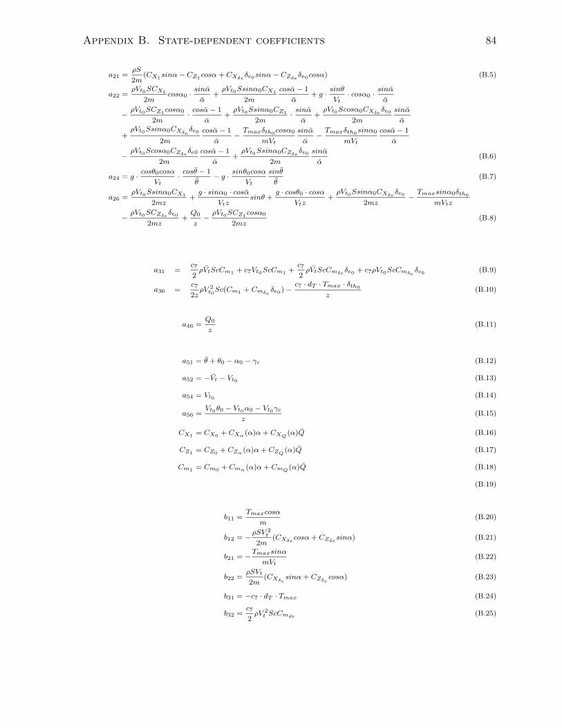
Appendix B. State-dependent coefficients 84
a21 =ρS
2m(CX1
sinα− CZ1cosα+ CXδeδe0sinα− CZδeδe0cosα) (B.5)
a22 =ρVt0SCX1
2mcosα0 ·
sinα
α+ρVt0Ssinα0CX1
2m
cosα− 1
α+ g ·
sinθ
Vt· cosα0 ·
sinα
α
−ρVt0SCZ1
cosα0
2m·cosα− 1
α+ρVt0Ssinα0CZ1
2m·sinα
α+ρVt0Scosα0CXδeδe0
2m
sinα
α
+ρVt0Ssinα0CXδe δe0
2m
cosα− 1
α−Tmaxδth0
cosα0
mVt
sinα
α−Tmaxδth0
sinα0
mVt
cosα− 1
α
−ρVt0Scosα0CZδeδe0
2m
cosα− 1
α+ρVt0Ssinα0CZδeδe0
2m
sinα
α(B.6)
a24 = g ·cosθ0cosα
Vt·cosθ − 1
θ− g ·
sinθ0cosα
Vt
sinθ
θ(B.7)
a26 =ρVt0Ssinα0CX1
2mz+g · sinα0 · cosα
Vtzsinθ +
g · cosθ0 · cosαVtz
+ρVt0Ssinα0CXδeδe0
2mz−Tmaxsinα0δth0
mVtz
−ρVt0SCZδeδe0
2mz+Q0
z−ρVt0SCZ1
cosα0
2mz(B.8)
a31 =c7
2ρVtScCm1 + c7Vt0ScCm1 +
c7
2ρVtScCmδeδe0 + c7ρVt0ScCmδe δe0 (B.9)
a36 =c7
2zρV 2t0Sc(Cm1 + Cmδe δe0 )−
c7 · dT · Tmax · δth0
z(B.10)
a46 =Q0
z(B.11)
a51 = θ + θ0 − α0 − γc (B.12)
a52 = −Vt − Vt0 (B.13)
a54 = Vt0 (B.14)
a56 =Vt0θ0 − Vt0α0 − Vt0γc
z(B.15)
CX1 = CX0 + CXα (α)α+ CXQ (α)Q (B.16)
CZ1 = CZ0 + CZα (α)α+ CZQ (α)Q (B.17)
Cm1 = Cm0 + Cmα (α)α+ CmQ (α)Q (B.18)
(B.19)
b11 =Tmaxcosα
m(B.20)
b12 = −ρSV 2
t
2m(CXδecosα+ CZδesinα) (B.21)
b21 = −Tmaxsinα
mVt(B.22)
b22 =ρSVt
2m(CXδe sinα+ CZδe cosα) (B.23)
b31 = −c7 · dT · Tmax (B.24)
b32 =c7
2ρV 2t ScCmde (B.25)
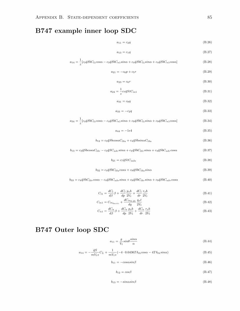
Appendix B. State-dependent coefficients 85
B747 example inner loop SDC
a11 = c2q (B.26)
a13 = c1q (B.27)
a14 =1
z[c3qSbCl1cosα− c3qSbCn1sinα+ c4qSbCl1sinα+ c4qSbCn1cosα] (B.28)
a21 = −c6p+ c5r (B.29)
a23 = c6r (B.30)
a24 =1
zc7qScCm1 (B.31)
a31 = c8q (B.32)
a33 = −c2q (B.33)
a34 =1
z[c4qSbCl1cosα− c4qSbCn1sinα+ c9qSbCl1sinα+ c9qSbCn1cosα] (B.34)
a44 = −1e4 (B.35)
b12 = c3qSbcosαClδa + c4qSbsinαClδa (B.36)
b13 = c3qSbcosαClδr − c3qSCnδrsinα+ c4qSbClδrsinα+ c4qSbCnδrcosα (B.37)
b21 = c7qScCmδe (B.38)
b32 = c4qSbClδacosα+ c9qSbClδasinα (B.39)
b33 = c4qSbClδrcosα− c4qSbCnδrsinα+ c9qSbClδrsinα+ c9qSbCnδrcosα (B.40)
Cl1 =dCl
dββ +
dCl
dp
psb
2Vt+dCl
dr
rsb
2Vt(B.41)
Cm1 = Cmbasic +dCm0.25
dq
qsc
2Vt(B.42)
Cn1 =dCn
dββ +
dCn
dp
psb
2Vt+dCn
dr
rsb
2Vt(B.43)
B747 Outer loop SDC
a11 =g
Vtsinθ
sinα
α(B.44)
a14 = −qS
mVtzCL +
1
mVtz(−4 · 0.0436Tδthcosα− 4Tδthsinα) (B.45)
b11 = −cosαsinβ (B.46)
b12 = cosβ (B.47)
b13 = −sinαsinβ (B.48)
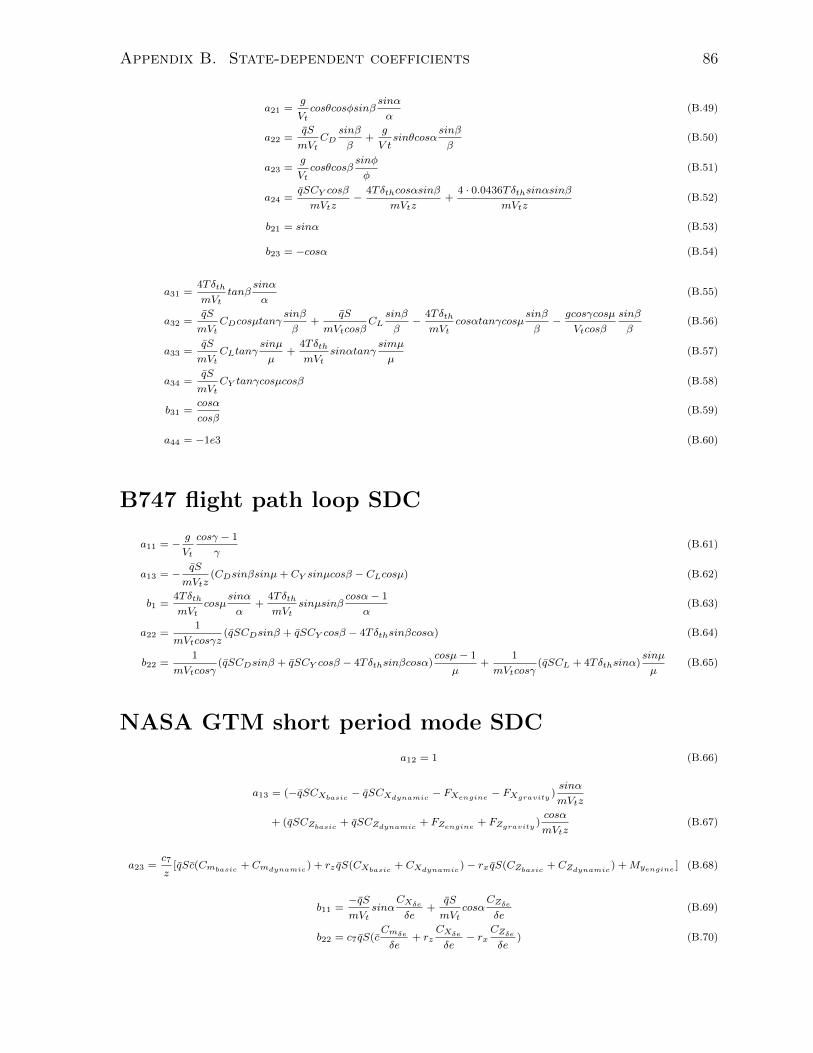
Appendix B. State-dependent coefficients 86
a21 =g
Vtcosθcosφsinβ
sinα
α(B.49)
a22 =qS
mVtCD
sinβ
β+
g
V tsinθcosα
sinβ
β(B.50)
a23 =g
Vtcosθcosβ
sinφ
φ(B.51)
a24 =qSCY cosβ
mVtz−
4Tδthcosαsinβ
mVtz+
4 · 0.0436Tδthsinαsinβ
mVtz(B.52)
b21 = sinα (B.53)
b23 = −cosα (B.54)
a31 =4Tδth
mVttanβ
sinα
α(B.55)
a32 =qS
mVtCDcosµtanγ
sinβ
β+
qS
mVtcosβCL
sinβ
β−
4Tδth
mVtcosαtanγcosµ
sinβ
β−gcosγcosµ
Vtcosβ
sinβ
β(B.56)
a33 =qS
mVtCLtanγ
sinµ
µ+
4Tδth
mVtsinαtanγ
simµ
µ(B.57)
a34 =qS
mVtCY tanγcosµcosβ (B.58)
b31 =cosα
cosβ(B.59)
a44 = −1e3 (B.60)
B747 flight path loop SDC
a11 = −g
Vt
cosγ − 1
γ(B.61)
a13 = −qS
mVtz(CDsinβsinµ+ CY sinµcosβ − CLcosµ) (B.62)
b1 =4Tδth
mVtcosµ
sinα
α+
4Tδth
mVtsinµsinβ
cosα− 1
α(B.63)
a22 =1
mVtcosγz(qSCDsinβ + qSCY cosβ − 4Tδthsinβcosα) (B.64)
b22 =1
mVtcosγ(qSCDsinβ + qSCY cosβ − 4Tδthsinβcosα)
cosµ− 1
µ+
1
mVtcosγ(qSCL + 4Tδthsinα)
sinµ
µ(B.65)
NASA GTM short period mode SDC
a12 = 1 (B.66)
a13 = (−qSCXbasic − qSCXdynamic − FXengine − FXgravity )sinα
mVtz
+ (qSCZbasic + qSCZdynamic + FZengine + FZgravity )cosα
mVtz(B.67)
a23 =c7
z[qSc(Cmbasic + Cmdynamic ) + rz qS(CXbasic + CXdynamic )− rxqS(CZbasic + CZdynamic ) +Myengine ] (B.68)
b11 =−qSmVt
sinαCXδeδe
+qS
mVtcosα
CZδeδe
(B.69)
b22 = c7qS(cCmδeδe
+ rzCXδeδe
− rxCZδeδe
) (B.70)
Bibliography
[1] Application of multivariable control theory to aircraft control laws. final report:
Multivariable control design guidelines. Technical Report ADA315259, Honeywell
Inc., Ma 1996.
[2] F.A. Almeida and D Leissling. Fault-tolerant model predictive control with flight
test results on ATTAS. In Proceedings of the AIAA Guidance, Navigation and
Control Conference and Exhibit, AIAA-2009-5621, Chicago, IL, 2009.
[3] H. Alwi and C. Edwards. Fault tolerant control using sliding modes with on-line
control allocation. Automatica, 44(7):1859–1866, 2008.
[4] H. Alwi, C. Edwards, O. Stroosma, and J.A. Mulder. Piloted sliding mode FTC sim-
ulator evaluation for the ELAL flight 1862 incident. In AIAA Guidance, Navigation
and Control Conference and Exhibit, AIAA-2008-7157, Honolulu, Hawaii, August
2008.
[5] A. Bogdanov, M. Carlsson, G. Harvey, J. Hunt, D. Kieburtz, R. V. D. Merwe, and
E. Wan. State-dependent riccati equation control of a small unmanned helicopter.
In AIAA Guidance, Navigation, and Control Conference and Exhibit, 2003.
[6] Charu Chawla and Radhakant Padhi. Reactive Obstacle Avoidance of UAVs with
Dynamic Inversion based partial integrated guidance and control. In AIAA Guid-
ance, Navigation, and Control Conference, number AIAA 2010-7729, Toronto, On-
tario, 2-5 August 2010.
[7] Tayfun Cimen. State-dependent riccati equation (SDRE) control: A survey. In
87
Bibliography 88
Proceedings of the 17th World Congress The International Federation of Automatic
Control, pages 3761–3775, Seoul, Korea, July 6-11 2008.
[8] Tayfun Cimen. Development and validation of a mathematical model for control of
constrained non-linear oil tanker motion. Mathematical and Computer Modelling of
Dynamical Systems, 15(1):17–49, Feb. 2009.
[9] Tayfun Cimen. Systematic and effective design of nonlinear feedback controllers via
the state-dependent Riccati equation (SDRE) method. Annual Reviews in Control,
34:32–51, 2010.
[10] Tayfun Cimen. Systematic and effective design of nonlinear feedback controllers via
the state-dependent riccati equation (SDRE) method. Annual Reviews on Control,
34:32–51, 2010.
[11] James R. Cloutier. State-dependent Riccati equation techniques: an overview. In
Proceedings of American Control Conference, Albuquerque, New Mexico, June 1997.
[12] J.R. Cloutier, C. N. D’Souza, and C.P. Mracek. Nonlinear regulation and nonlinear
H∞ control via the state-dependent riccati equation technique: Part 1, Theory. In
Proceedings of the International conference on Nonlinear Problems in Aviation and
Aerospace, Daytona Beach, FL, May 1996.
[13] J.R. Cloutier and D. T. Stansbery. Nonlinear, hybrid bank-to-turn/skid-to-turn
autopilot design. In AIAA Guidance, Navigation and Control Conference, Montreal,
Canada, 6-9 August 2001.
[14] R. P. G. Collinson. Fly-by-wire flight control. Computing and Control Engineering
journal, 10:141–152, 1999.
[15] Fabio A. de Almeida and Dirk Leissling. Fault-tolerant flight control system using
model predictive control. In Brazilian Symposium on Aerospace Eng. & Applications,
S. J. Campos, SP, Brazil, September 2009.
[16] Christopher Edwards, Thomas Lombaerts, and Hafid Smaili. Fault Tolerant Flight
Control, volume Lecture Notes in Control and Information Sciences, Vol. 399.
Bibliography 89
Springer, 2010.
[17] J.S. Eterno, J.L. Weiss, D.P. Looze, and A.S. Willsky. Design issues for fault tolerant-
restructurable aircraft control. In 24th IEEE conference on decision and control, Ft.
Lauderdale, FL, December 1985.
[18] Chris Fielding. The design of fly-by-wire flight control systems. BAE Systems, 2000.
[19] B. Friedland. Advanced Control System Design. Prentice Hall, 1996.
[20] N. Frink, S. Pirzadeh, J. Morrison, H. Atkins, S. Viken, and J. Morrison. CFD
assessment of aerodynamic degradation of a subsonic transport due to airframe
damage. In 48th AIAA Aerospace Sciences Meeting, Orlando, FL, 4-7 Jan. 2010.
[21] Chen Gao, Huifeng Li, and Ping Zhang. Re-entry tracking control via state-
dependent riccati equations. In AsiaSim 2007, volume 5, pages 112–118. 2007.
[22] C. R. Hanke. The simulation of a large jet transport aircraft volume I: Mathematical
model. Technical Report NASA CR-1756, NASA, March 1971.
[23] C.R. Hanke and D.R. Nordwall. The siumlation of a jumbo jet transport aircraft
volume II: Modeling data. Technical Report D6-30643, NASA, September 1970.
[24] A. Isidori. Nonlinear control systems. Berlin: Springer-Verlag, 1995.
[25] D.A. Joosten, T.J.J. van den Boom, and T.J.J. Lombaerts. Fault-tolerant control
using dynamic inversion and model-predictive control applied to an aerospace bench-
mark. In Proceedings of the 17th World Congress The International Federation of
Automatic Control, Seoul, Korea, July 2008.
[26] M.M. Kale and A.J. Chipperfield. Stabilized MPC formulations for robust reconfig-
urable flight control. Control Engineering Practice, 13(6):771–788, 2005.
[27] H. Khalil. Nonlinear systems. Prentice Hall, 2002.
[28] Ki-Seok Kim, Keum-Jin Lee, and Youdan Kim. Reconfigurable flight control system
design using direct adaptive method. Journal of guidance, control and dynamics,
26(4):543–550, July 2003.
[29] Eugene Lavretsky and Ross Gadient. Predictor-based model reference adaptive
Bibliography 90
control. Journal of Guidance, Control and Dynamics, 33(4):1195–1201, July-August
2010.
[30] T.J.J. Lombaerts, H.O. Huisman, Q.P. Chu, J.A. Mulder, and D.A. Joosten. Flight
control reconfiguration based on online physical model identification and nonlinear
dynamic inversion. Journal of guidance, control, and dynamics, 32(3):727–748, 2009.
[31] J. Maciejowski and C.N. Jones. MPC fault-tolerant flight control case study: Flight
1862. In Proceedings of the 5th IFAC symposium on fault detection, supervision and
safety for technical processes, pages 121–126, Washington, D.C., 9-11 June 2003.
[32] A. Marcos and G. Balas. Development of linear-parameter-varying models for air-
craft. Journal of guidance, control and dynamics, 27(2):218–228, March 2004.
[33] P. K. Menon, S. S. Vaddi, and P. Sengupta. Robust landing guidance law for impaired
aircraft. In AIAA Guidance, Navigation, and Control Conference, Toronto, August
2010.
[34] P.K. Menon, T. Lam, L.S. Crawford, and V.H.L. Cheng. Real-time computational
methods for SDRE nonlinear control of missiles. In American control conference,
pages 232 – 237, Anchorage, AK, 8-10 May 2002.
[35] T. Miksch, A. Gambier, and E. Badreddin. Real-time implementation of fault-
tolerant control using model predictive control. In Proceedings of the 17th IFAC
World Congress, pages 11136–11141., Seoul, Korea, 2008.
[36] R. Montoya, W. Howell, W.T. Bundick, A. Ostroff, R. Hueschen, and C. Belcastro.
Restructurable controls. Technical Report CP-2277, NASA, 1982.
[37] C. Mracek and J. Cloutier. Full envelope missile longitudinal autopilot design using
the state-dependent riccati equation method. In AIAA Guidance, Navigation, and
Control Conference, New Orleans, LA, 11-13 August 1997.
[38] C.P. Mracek and J.R. Cloutier. Control designs for the nonlinear benchmark problem
via the state-dependent riccati equation method. International Journal of Robust
and Nonlinear Control, 8:401–433, 1998.
Bibliography 91
[39] C.P. Mracek and J.R. Cloutier. Control designs for the nonlinear benchmark problem
via the state-dependent riccati equation method. International Journal of Robust
and Nonlinear Control, 8:401–433, 1998.
[40] Marcello R. Napolitano, Younghwan An, and Brad A. Seanor. A fault tolerant
flight control system for sensor and actuator failures using neural networks. Aircraft
Design, 3(2):103–128, June 2000.
[41] T.S. No, B.M. Min, R.H. Stone, and K.C. Wong. Control and simulation of arbitrary
flight trajectory-tracking. Control Engineering Practice, 13(5):601–612, May 2005.
[42] T.S. No, B.M. Min, R.H. Stone, and K.C. Wong. Control and simulation of arbitrary
flight trajectory-tracking. Control Engineering Practice, 13:601–612, 2005.
[43] G. D. Padfield and G. D. Padfield. The birth of flight control: An engineering
analysis of the wright brothers’ 1902 glider. The aeronautical journal, pages 697–
718, December 2003.
[44] J.D. Pearson. Approximation methods in optimal control. Journal of Electronics
and Control, 13:453–469, 1962.
[45] M. Rauw. FDC 1.2a simulink toolbox for flight dynamics and control analysis.
Technical report, 2001.
[46] Jason Levin Ross Gadient and Eugene Lavretsky. Comparison of model reference
adaptive controller designs applied to the NASA generic transport model. In AIAA
Guidance, Navigation, and Control Conference, number AIAA 2010-8406, Toronto,
ON, 2-5 August 2010.
[47] D. Shin, G. Moon, and Y. Kim. Design of reconfigurable flight control system using
adaptive sliding mode control: actuator fault. In Proceedings of the Institution
of Mechanical Engineers, Part G (Journal of Aerospace Engineering), volume 219,
pages 321–328, 2005.
[48] Jong-Yeob Shin and I. Gregory. Robust gain-scheduled fault tolerant control for a
transport aircraft. In IEEE International Conference on Control Applications, pages
Bibliography 92
1209–1214, October 2007.
[49] Jong-Yeob Shin, N. Eva Wu, and Christine Belcastro. Adaptive linear parameter
varying control synthesis for actuator failure. Journal of guidance, control and dy-
namics, 27(5):787–794, September 2004.
[50] B.L. Stevens and F.L. Lewis. Aircraft Control and Simulation. John Wiley, 2nd
edition, 2003.
[51] M. Vidyasagar. Nonlinear systems analysis. Prentice Hall, 1993.
[52] A. Wernli and G. Cook. Suboptimal control for the nonlinear quadratic regulator
problem. Automatica, 11:75–84, 1975.
[53] G.X. Xu and H.H.T. Liu. Nonlinear fault-tolerant flight control design applied to
a loss-of-thrust aircraft. In AIAA Guidance, Navigation and Control Conference,
Portland, OR, 8-11 August 2011.
[54] G.X. Xu and H.H.T. Liu. Trajectory tracking design for a transport aircraft using
model reference adaptive control. In CASI 58th Aeronautics Conference, Montreal,
QC, April 26-28 2011.
[55] Dan Ye and Guang hong Yang. Adaptive fault-tolerant tacking control against
actuator faults with application to flight control. IEEE Transaction on control
systems technology, 14(6):108–8–1096, 2006.
[56] P. Zarchan. Tactical and Strategic Missile Guidance. AIAA, 2007.
[57] Youmin Zhang and Jin Jiang. Bibliographical review on reconfigurable fault-tolerant
control systems. Annual Reviews on Control, 32:229–252, 2008.
Top Related