


Languages
Pages
Legal

NONLINEAR ESTIMATION TECHNIQUES APPLIED TO ECONOMETRIC
PROBLEMS
A THESIS SUBMITTED TO
THE GRADUATE SCHOOL OF APPLIED AND NATURAL SCIENCES
OF
MIDDLE EAST TECHNICAL UNIVERSITY
BY
SERDAR ASLAN
IN PARTIAL FULFILMENT OF THE REQUIREMENTS
FOR
THE DEGREE OF MASTER OF SCIENCE
IN
ELECTRICAL AND ELECTRONICS ENGINEERING
NOVEMBER 2004

Approval of Graduate School of Natural and Applied Sciences.
______________________________
Prof. Dr. Canan ÖZGEN
Director
I certify that this thesis satisfies all the requirements as a thesis for the degree of
Master of Science.
______________________________
Prof. Dr. İSMET ERKMEN
Head of Department
This is to certify that we have read this thesis and that in our opinion it is fully
adequate, in scope and quality, as a thesis for the degree of Master of Science.
______________________________
Prof. Dr. Kerim DEMİRBAŞ
Supervisor
Examining Committee Members
Prof. Dr. Mübeccel DEMİREKLER (METU,EEE)______________________
Prof. Dr. Kerim DEMİRBAŞ (METU,EEE)______________________
Prof. Dr. Kemal LEBLEBİCİOĞLU (METU,EEE) ______________________
Assist. Prof. Dr. Ümit Özlale BİLKENT,ECON)______________________
Assist. Prof. Dr. Çağatay CANDAN (METU,EEE)______________________

iii
I hereby declare that all information in this document has been obtained and
presented in accordance with academic rules and ethical conduct. I also declare
that, as required by these rules and conduct, I have fully cited and referenced
all material and results that are not original to this work.
Name, Last Name : Serdar Aslan
Signature :
iv
ABSTRACT
NONLINEAR ESTIMATION TECHNIQUES APPLIED
TO ECONOMETRIC
Aslan, Serdar
M. Sc., Department of Electrical and Electronics Engineering
Supervisor: Prof. Dr. Kerim Demirbaş
November 2004, 62 pages
This thesis considers the filtering and prediction problems of nonlinear noisy
econometric systems. As a filter/predictor, the standard tool Extended Kalman Filter
and new approaches Discrete Quantization Filter and Sequential Importance
Resampling Filter are used. The algorithms are compared by using Monte Carlo
Simulation technique. The advantages of the new algorithms over Extended Kalman
Filter are shown.
Keywords: Discrete Quantization Filter, Sequential Importance Resampling Filter,
Extended Kalman Filter, Stochastic Calculus, Monte Carlo
v
ÖZ
DOĞRUSAL OLMAYAN KESTİRME
ALGORİTMALARININ EKONOMETRİK
PROBLEMLERE UYGULANMASI
Aslan, Serdar
M. Sc., Department of Electrical and Electronics Engineering
Supervisor: Prof. Dr. Kerim Demirbaş
November 2004, 62 sayfa
Bu tez doğrusal olmayan ekonometrik gürültülü sistemlerde gürültüden
arındırma ve tahmin yapma üzerinedir. Filtre ve öngörücü olarak standart gereç olan
Geliştirilmiş Kalman Algoritması ve yeni yaklaşımlar olan Zamanda Ayrık
Nicemleme Filtresi ve Ardışık Önem Tekrarlı Örnekleme Filtresi kullanıldı.
Algoritmalar birbiriyle Monte Carlo Similasyon tekniğiyle karşılaştırıldı.
Algoritmaların Geliştirilmiş Kalman Algoritmasından avantajlı yanları gösterildi.
Anahtar Kelimeler: Geliştirilmiş Kalman Filtresi, Zamanda Ayrık Nicemleme
Filtresi, Ardışık Önem Tekrarlı Örnekleme Filtresi, Olasılıksal Analiz, Monte Carlo.

vi
ACKNOWLEDGEMENTS
I would like to thank to my advisor, Professor Kerim Demirbaş, for his
assistance throughout the thesis.
My thesis was a combination of different science branches. In this respect I
have taken excellent feedback from different departments such as: Mathematics,
Economics, and Statistics.
In this respect, I would like to thank Professor Hayri Körezlioğlu for his
suggestions on stochastic calculus. He also directed me through choosing the
nonlinear dynamic systems from the field of economics.
I am also grateful to Assistant Professor Ümit Özlale for his various advices
on the economic systems being used.
Regarding the Matlab codes, I would like to thank Murat Tepegöz, Hüseyin
Yiğitler and Serdar Sutay for their kind help. Murat Tepegöz helped to me to
summarize the codes. Hüseyin Yiğitler and Serdar Sutay wrote the codes in an
alternative way such that I could compare my program output with theirs.
I am also grateful to Umut Orguner for assisting me in the theory of Extended
Kalman Filter and in Monte Carlo Simulations. I would also like to thank Assistant
Professor Çağatay Candan and Asaf Behzat Şahin for their valuable advices.
Assistant Professor Candan and Associate Professor Sencer Koç also helped me on
the numerical computation techniques of solving nonlinear equations.
Special thanks go to Prof. Dr. Mübeccel Demirekler for her help to continue
my master study.

vii
TABLE OF CONTENTS ABSTRACT_____________________________________________________iv ACKNOWLEDGEMENTS ________________________________________vi TABLE OF CONTENTS _________________________________________ vii LIST OF TABLES _______________________________________________ix LIST OF FIGURES ______________________________________________ x
1. INTRODUCTION ________________________________________________ 1
2. FIRST MODEL – FROM CONTINUOUS TIME TO DISCRETE TIME ____ 4 2.1 Discretization of the Model __________________________________________ 5
3. STOCHASTIC CALCULUS and APPLICATION TO THE CASE STUDY __ 7 3.1 STOCHASTIC DIFFERENTIAL EQUATIONS ________________________ 8 3.2 The Riemann Integral ______________________________________________ 9 3.3 The Riemann-Stieltjes Integral______________________________________ 10 3.4 LP Convergence and Convergence in Mean Square _____________________ 11 3.5 Simple Processes__________________________________________________ 12 3.6 Outline for the Definition of the Ito Stochastic Integral__________________ 12 3.7 The Ito Stochastic Integral of Simple Processes ________________________ 12 3.8 The Ito Stochastic Integral of General Processes _______________________ 13 3.9 Ito’s Lemma _____________________________________________________ 14 3.10 Solution of the Stochastic Differential Equation _______________________ 16 3.11 Uniqueness of the Solution of the Stochastic Differential Equation _______ 19
4. DQF ALGORITHM ______________________________________________ 21 4.1 DQF ____________________________________________________________ 21
4.1.1 Obtaining a Trellis Diagram ___________________________________________ 22 4.1.2 Assigning Metrics to the Nodes of the Trellis Diagram ______________________ 22 4.1.3 Choosing the Highest Metric for the Determination of the Best Path ____________ 24
4.2 Quantization of the random variable _________________________________ 25 5. EKF___________________________________________________________ 27
6. APPLICATION OF EKF TO ECONOMETRICS ______________________ 29
7. PARTICLE FILTERS-SIR ALGORITHM ___________________________ 31 7.1 Derivation of the SIS and SIR algorithm ______________________________ 33
8. SIMULATIONS OF FILTERING AND PREDICTION EXPERIMENTS __ 37 8.1 General Outline __________________________________________________ 37 8.2 Filtering Tools____________________________________________________ 38 8.3 Prediction Tools __________________________________________________ 38 8.4 Error Criteria and Monte Carlo Simulations __________________________ 38
viii
8.4.1 Filtering Error ______________________________________________________ 39 8.4.1.1 Error in RN Spaces: _______________________________________________ 39 8.4.1.2 Errors in the Experiments __________________________________________ 39
8.4.2 Prediction Error _____________________________________________________ 40 8.5 Simulations ______________________________________________________ 41
8.5.1 Filtering ___________________________________________________________ 43 8.5.1.1 _______________________________________________________________ 43 8.5.1.2 _______________________________________________________________ 43 8.5.1.3 _______________________________________________________________ 44 8.5.1.4 _______________________________________________________________ 45 8.5.1.5 _______________________________________________________________ 46
8.5.2 Prediction _________________________________________________________ 47 9. SIMULATIONS OF FILTERING EXPERIMENTS FOR STOCHASTIC
GROWTH MODELS __________________________________________ 49
10. CONCLUSION__________________________________________________ 52
11. REFERENCES _________________________________________________ 54
12. APPENDIX ____________________________________________________ 57

ix
LIST OF TABLES TABLES Table 1 Monte Carlo results-Errors of the algorithms versus change of the variance
of w __________________________________________________________ 43 Table 2 Monte Carlo results-Errors of the algorithms versus change of the variance
of w __________________________________________________________ 44 Table 3 Monte Carlo results-Errors of the algorithms versus change of the variance
of w __________________________________________________________ 44 Table 4 Monte Carlo results-Errors of the algorithms for the variance of w=5 ____ 46 Table 5 Monte Carlo results-Errors of the algorithms SIR and EKF ____________ 48 Table 6 Monte Carlo results-Errors of the algorithms SIR and EKF ____________ 51

x
LIST OF FIGURES
Figure 1 ...................................................................................................................... 45
1
CHAPTER 1
INTRODUCTION
In electrical and electronics engineering, there are many dynamical system
representations, which include noise components. In such cases, one of the primary
goals is to remove the noise component from the measurement and/or try to predict
the next state of the system. If the problem at hand can be written in a linear
Gaussian system form, then the Kalman Filter emerges as the optimal methodology.
However, when the system has nonlinear characteristics, then the Extended Kalman
Filter (EKF henceforth) should be employed1. However, the estimation of nonlinear
systems should by no means restricted to using only EKF. As discussed in [3] and
[25] in details, Discrete Quantization Filter and Sequential Importance Resampling
(SIR) filters can conveniently be used
Based on the above discussion, there are three features of this study:
1) Control theory approaches are applied to the field of econometrics:
2) Stochastic Calculus has been introduced within the context of a stochastic Ito
process, which is used basically in the asset pricing models
3) Two relatively unknown algorithms, DQF and SIR filter are introduced and
compared with the EKF. As it will be clear, some cases where these two
alternatives are superior to EKF are presented.
To begin with, state space representations are convenient to describe the
dynamical systems. It is straightforward to obtain the dynamics of the model from
the differential equation representation of the nonnoisy systems. [4] However, in
noisy systems, the description of the system is generally is introduced within the
state space representation. In such systems, the noise is assumed to be generally
additive. But thanks to the stochastic calculus, we have a more general perspective.
1 For a detailed discussion on Kalman Filter see [1] and [2]
2
The assumptions of the noise structure can be made directly in a differential equation
form. Then, the differential equations with noise are solved by employing stochastic
calculus. For a general treatment of the subject stochastic calculus, the reader is
referred to [5].
Consequently, the study briefly described above is composed of the following
parts:
1) Introduction
2) First Model – From Continuous Time to Discrete Time
3) Stochastic Calculus and Application to the Case Study
4) DQF Algorithm
5) EKF Algorithm
6) Application of EKF to the Econometric Problem
7) Particle Filters-SIR Algorithm
8) Simulations of the First model
9) Simulations of the Second Model
The second section explains how the discrete-time nonlinear noisy system
representation of the first model is obtained from continuous time representation.
The dynamical system is based on obtaining the expression for the price of one risky
asset (stock). Since the primary goal of this study is not to focus on the details of the
derivation, just a succinct introduction is given in this section.
In the third section named “Stochastic Calculus and Application to the Case
Study”, the necessary background to understand the basics of Stochastic Calculus is
explained. Then it is shown, how the continuous time solution has been obtained
from the stochastic differential equations.
In the fourth section, named “DQF Algorithm”, the basics of the algorithms
proposed by Demirbaş [3] are explained. Although not widely known, this algorithm
is capable to lead to better results than the standard EKF algorithm. The next two
sections briefly discuss the EKF algorithm. In the former, EKF for discrete time
cases is explained. In the latter section, the algorithm is applied to the nonlinear
dynamic system of the model derive in the previous sections.
The seventh section elaborates the particle filters. It gives the derivation of
the Sequential Importance Sampling (SIS) filter along with its proof. Then, the SIR
filter, which is also employed in this study, is easily derived from SIS filter.

3
The eighth section displays the simulation results of the filtering and
prediction algorithms of the benchmark model introduced before.
The next section presents the simulation results of the filtering algorithm of
the second model, which basically examines productivity shocks and capital
accumulation within a stochastic growth model. The final section concludes.

4
CHAPTER 2
FIRST MODEL – FROM CONTINUOUS TIME TO DISCRETE TIME
In a conventional asset pricing model, the price of one share of the risky asset
(stock) is described by the following stochastic differential equation (2.1).
)(tdX = c )(tX δ+dt )(tX )(tdB (2.1)
)(tX : The price )(tX is called risky asset. It is also named as stock.
c : The constant c is the mean rate of return.
δ : The parameter δ denotes volatility.
B : )0),(( ≥= ttBB represents the Brownian motion. [6]
The differential formula in equation (2.1) is similar to the expressions used in
differential calculus with the important exception that there is a term )(tdB , which
represents the stochastic part. Such a term makes the usage of the stochastic calculus
necessary, which has also been widely used in the field of econometrics.
In the third section, a necessary background for a thorough understanding of
the above mentioned subject is given. As the third section shows in details, the
solution to the above given formula for X(t) is given by:
)()5.0( 2
)0())(,()( tBtceXtBtftX δδ +−== (2.2)
(2.2) is an exponential function which is randomly perturbed. It is also named
as Geometric Brownian Motion. )0(X is assumed to be independent of .B If the
5
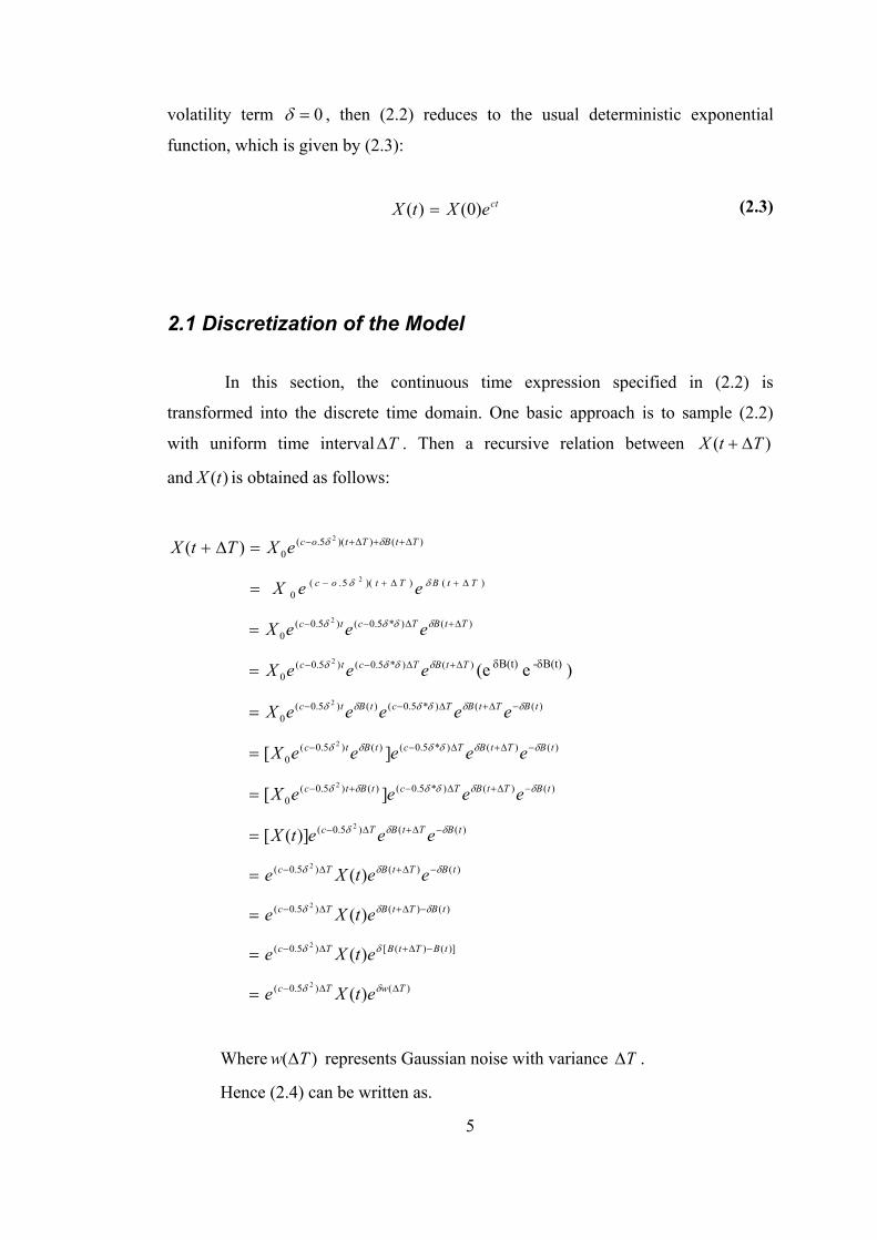
volatility term 0=δ , then (2.2) reduces to the usual deterministic exponential
function, which is given by (2.3):
cteXtX )0()( = (2.3)
2.1 Discretization of the Model
In this section, the continuous time expression specified in (2.2) is
transformed into the discrete time domain. One basic approach is to sample (2.2)
with uniform time interval T∆ . Then a recursive relation between )( TtX ∆+
and )(tX is obtained as follows:
)())(5.(
0
2
)( TtBTtoceXTtX ∆++∆+−=∆+ δδ
)())(5.(0
2 TtBTtoc eeX ∆+∆+−= δδ
)()*5.0()5.0(0
2 TtBTctc eeeX ∆+∆−−= δδδδ
)()*5.0()5.0(0
2 TtBTctc eeeX ∆+∆−−= δδδδ (e δB(t) e -δB(t) )
)(()*5.0()()5.0(0
2 tBTtBTctBtc eeeeeX δδδδδδ −∆+∆−−=
)()()*5.0()()5.0(0 ][
2 tBTtBTctBtc eeeeeX δδδδδδ −∆+∆−−=
)()()*5.0()()5.0(0 ][
2 tBTtBTctBtc eeeeX δδδδδδ −∆+∆−+−=
)(()5.0( 2
)]([ tBTtBTc eeetX δδδ −∆+∆−=
)()()5.0( )(2 tBTtBTc eetXe δδδ −∆+∆−=
)()()5.0( )(2 tBTtBTc etXe δδδ −∆+∆−=
)]()([)5.0( )(2 tBTtBTc etXe −∆+∆−= δδ
)()5.0( )(2 TwTc etXe ∆∆−= δδ
Where )( Tw ∆ represents Gaussian noise with variance T∆ .
Hence (2.4) can be written as.
6
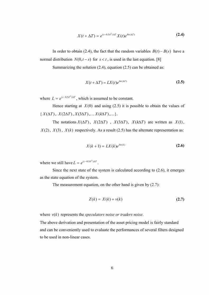
)( TtX ∆+ )()5.0( )(2 TwTc etXe ∆∆−= δδ (2.4)
In order to obtain (2.4), the fact that the random variables )()( sBtB − have a
normal distribution ),0( stN − for ts < , is used in the last equation. [8]
Summarizing the solution (2.4), equation (2.5) can be obtained as:
)()()( TwetLXTtX ∆=∆+ δ (2.5)
where TceL ∆−= )5.0( 2δ , which is assumed to be constant.
Hence starting at )0(X and using (2.5) it is possible to obtain the values of
{ )( TX ∆ , )2( TX ∆ , )3( TX ∆ ,… )( TkX ∆ ,…}.
The notations )( TX ∆ , )2( TX ∆ , )3( TX ∆ , )( TkX ∆ are written as )1(X ,
)2(X , )3(X , )(kX respectively. As a result (2.5) has the alternate representation as:
)()()1( kwekLXkX δ=+ (2.6)
where we still have TceL ∆−= )5.0( 2δ .
Since the next state of the system is calculated according to (2.6), it emerges
as the state equation of the system.
The measurement equation, on the other hand is given by (2.7):
)()()( kvkXkZ += (2.7)
where )(kv represents the speculators noise or traders noise.
The above derivation and presentation of the asset pricing model is fairly standard
and can be conveniently used to evaluate the performances of several filters designed
to be used in non-linear cases.
7
CHAPTER 3
STOCHASTIC CALCULUS and APPLICATION TO THE CASE STUDY
This section briefly introduces stochastic differential calculus. Before
discussing the implications it should be mentioned that, the reader, who is not
familiar with stochastic processes is referred to [9].
First, it is important to remind the definition and the interpretation of
stochastic differential equations. The integral that is written in the form of (3.1)
∫t
sdBsXsb0
)())(,( (3.1)
is called Ito Integral. This integral representation differs in two ways from its
counterparts:
1) We have dB(s) instead of ds.
2) B is not a deterministic function but a stochastic one.
The formal definition of (3.1) is given in the subsection 3.8.
The subsection 3.2 “The Riemann Integral” reminds the reader the formal
definition of Riemann Integral. The subsection 3.3 named “The Riemann-Stieltjes
Integral” is a simple extension of Riemann Integral. The reason to introduce this
integral type is the connection between the Ito Integral and Riemann-Stieltjes
Integral
The subsections 3.4 and 3.5, which are “Lp Convergence and Mean Square
Convergence” and “Simple Processes” respectively, define convergence types of
stochastic processes, which are used in the definition of Ito integral,

8
The subsection 3.7, namely the “Ito Integral of Simple Processes” first
defines the Ito Integral for a restricted class of processes. Then the subsection 3.8
“Ito Integral of General Processes” enlarges the definition of the Ito Integral for a
wider class of processes. At this stage, the theoretical implication of the Ito integral
is concluded with a brief discussion. After this section, practical aspects of stochastic
calculus are introduced and applied to econometrics, which was explained in the
second section.
The subsection 3.9 Ito Lemma is the basic tool, which is needed to solve the
stochastic differential equations.
The subsection 3.10 is an application of the Ito Lemma to the case study,
which is a standard stochastic growth model.
Finally, the subsection 3.11 discusses the uniqueness problem of the solution,
which is obtained in the section 3.10
3.1 STOCHASTIC DIFFERENTIAL EQUATIONS
In stochastic calculus, a basic expression takes the following form:
dBtxtbdttXtatdX ))(,())(,()( += (3.2)
where t is the independent variable, ),( xta and ),( xtb are deterministic functions,
and )0),(( ≥= ttBB is the Brownian motion. It is easy to see that, for 0),( =xtb ,
(3.2) reduces to the usual deterministic differential equation.
In the stochastic calculus (3.2), can also be interpreted as:
∫∫ ++=tt
sdBsXsbdssXsaXtX00
)())(,())(,()0()( , Tt ≤≤0 (3.3)
In this notation, dssXsat
∫0
))(,( is the usual Riemann integral. The integrand
function ))(,( sXsb and the integrating function )(sB are stochastic processes.
9
Integrals of the form ∫t
sdBsXsb0
)())(,( should be interpreted differently. Ito process
offers such an interpretation. Since Ito interpretation is the most commonly used
process, it will be employed throughout the study. However, it should be reminded
that there are also other interpretations like the Stratonovich interpretation. In some
cases, it is better to use Stratonovich interpretation, as expressed in [10]
The next section Riemann integral is defined formally.
3.2 The Riemann Integral
The classical integration technique is the Riemann integral. The standard
notation is shown in (3.4).
tdtfTx
x∫=
=0
)( (3.4)
where t denotes the independent variable. f is the function to be integrated. 0 and T
are the limits of integration. The definition of Riemann Integral is as follows:
1) First the interval ],0[ T is partitioned as:
Let Ttttt nnn =<<<<= −110 ...0:τ be the mentioned partition of the
interval ],0[ T .
2) Choose iy , iii tyt ≤≤−1 for .,...,1 ni =
3) Let )()( 11
−=
−= ∑ ii
n
iin ttyfS
4) If SSnn=
∞→lim exists, for some S and for each possible partition nτ and iy as
0)( 1 →− −ii tt , then tdtfSTx
x∫=
=
=0
)( .
While Riemann integration technique is used extensively in several areas it is
not appropriate for analyzing the dynamics of the systems with random terms. For
that purpose, Ito’s Stochastic Integral offers a solution.
10
The Riemann-Stieltjes Integral, which is a simple extension of Riemann
Integral, is discussed in the next section.
3.3 The Riemann-Stieltjes Integral
Definition [11]
1) Let Ttttt nnn =<<<<= −110 ...0:τ be a partition of the interval [0,1].
2) Choose iy , iii tyt ≤≤−1 for .,...,1 ni =
3) Let f and g be two real-valued functions on [0,1] and define (3.5)
)()( 1−−=∆ iii tgtgg , i=1,…,n. (3.5)
4) The Riemann-Stieltjes sum corresponding to nτ and is given by (3.6)
)]()([)()()( 111
−==
−=∆== ∑∑ ii
n
iii
n
iinnn tgtgyfgyfSS τ .
(3.6)
5) If the limit nnS
∞→lim exists and S is independent of the choice of the
partitions nτ and iy as 0)( 1 →− −ii tt , then S is called the Riemann-Stieltjes integral
of f with respect to g on [0,1]. Symbolically, it is written as (3.7).
∫=1
0
).()( tdgtfS (3.7)
Riemann-Stieltjes integral is just an extension of the classical Riemann
integral. It is reduced to the Riemann integral for g(t)=t. This integration technique is
also used in the probability theory. In these cases g is to be chosen as F, which is the
distribution function of a random variable. For example, (3.8) represents such a form:
∫∈
=∈Ax
xdFAxP )(}{ (3.8)
11
Although Ito’s stochastic integral is different from the Riemann-Stieltjes
integral, as the proceeding sections will show, there are connections as well. These
connections are shown after the definition of the Ito stochastic integral. In the next
section, some mathematical terms, which are necessary to understand the definition
of the Ito integral, are introduced.
3.4 LP Convergence and Convergence in Mean Square
If nX and X belong to pL and 0→− pn XXE , then }{ nX is said to
converge in p’th mean to X. For 1=p , it is simply called convergence in mean; for
2=p , on the other hand, the process is generally termed as convergence in mean
square or in quadratic mean.[12] This process is employed for the definition of Ito
Integral.
In the above definition, E is the usual expectations operator while pL is the
space of functions, for which the pL norm is finite.
12
3.5 Simple Processes
The stochastic process ]),0[),(( TttCC ∈= is said to be “simple process” if it
satisfies the following properties:
There exists a partition: Ttttt nnn =<<<<= −110 ...0:τ , and a sequence
),...,1,( niZi = of random variables such that: [13]
nZtC =)( if ,Tt =
iZtC =)( if ,1 ii ttt <≤− .,...,1 ni =
3.6 Outline for the Definition of the Ito Stochastic Integral
As mentioned before, the Ito Integral employs the mean square convergence.
For the definition of the Ito stochastic integral, the following way will be tracked:
1. The integrand function is first assumed to be a simple process.
2. The Ito integral of the simple processes is given.
3. The integrand function is assumed to be a general process.
4. The Ito integral of the general process is defined via the simple processes.
3.7 The Ito Stochastic Integral of Simple Processes
The Ito stochastic integral of a simple process C on ],0[ T is given by (3.9).
BZtBtBtCsdBsCn
iiiii
n
ii
T
∑∑∫=
−=
− ∆=−=1
11
10
))()(()(:)()( (3.9)
where )( 1−= ii tCZ and ))()(( 1−−=∆ iii tBtBB .
13
The Ito stochastic integral of a simple process C on [0,t], kk ttt ≤≤−1 , is
given by (3.10).
))()(()()()(:)()( 1
1
10],0[
0−
−
=
−+∆== ∑∫∫ kk
k
iii
T
t
t
tBtBZBZsdBsIsCsdBsC (3.10)
, 1)(],0[ =sI t for [ ]ts ,0∈ and 0)(],0[ =sI t otherwise.
When comparing (3.9) with the Riemann-Stieltjes sum notation (3.6), it is
easily seen that 1−= ii ty . Furthermore, “g” corresponds to Brownian motion. Hence
the Ito stochastic integral is the Riemann-Stieltjes sum, where the intermediate points
iy are chosen at the left end points of the intervals ],[ 1 ii tt − .
This concludes the definition of the Ito integral for simple processes, which
can be regarded as the corner stone for the general stochastic integration.
3.8 The Ito Stochastic Integral of General Processes
The Ito stochastic integral is defined for simple processes in section 3.7. In
this section, however, the integrand process will be from a wider class of function
space. But the following restrictions are put for this class:
Assumptions on the Integrand Process C:
1. C is adapted to Brownian motion on [0,T], i.e. C(t) is a function of B(s)
ts ≤ .
2. The integral (3.11) is finite.
dssECT
∫0
2)( (3.11)
Let C be a process satisfying the above additional assumptions. Then, one can
find a sequence (C(n)) of simple processes such that the following statement holds.
See [14], for the proof of this statement.
00
1=∆∑ =
BZwhere ii i
14
0])()([0
2)( →−∫ dssCsCET
n (3.12)
Hence, the simple processes )(nC converge in mean square sense to the
integrand process C. Using (3.10), we can calculate the Ito integrals )( )(nt CI of these
simple processes. Hence we have a new sequence { )( )1(CIt , )( )2(CIt ,…}. This new
sequence converges to a unique process, which van be conveniently called as )(CI
on [0,T] Then, we can write (3.13) as[15]:
.0)]()([sup 2)(
0→−
≤≤
ntt
TtCICIE (3.13)
The mean square limit )(CI is called the Ito stochastic integral of C. It is
denoted by (3.14)[14]
)()()( sdBsCCIt
ot ∫= , ].,0[ Tt ∈
(3.14)
This ends the formal definition for the Ito stochastic integral. In order to
apply the integral, however, the Ito Lemma should be introduced.
3.9 Ito’s Lemma
In this subsection, the Ito’s Lemma is introduced in order to apply the stochastic
integral that is defined above.
Ito’s Lemma:
Let ),( xtf be a function whose second order partial derivatives are
continuous. Then (3.15) is true.
∫∫ ++=−t
s
t
s
xdBxBxfdxxBxfxBxfsBsftBtf ())(,())](,(21))(,([))(,())(,( 2221
(3.15
)
15
where ts < . For the details of the lemma, please refer to [16].
dxxBxfxBxft
s
))](,(21))(,([ 221∫ +
(3.16)
∫t
s
xdBxBxf )())(,(2 (3.17)
The first integral (3.16) is a simple deterministic integral. The second integral
(3.17) is the aforementioned stochastic integral in section 3.8. Furthermore 21, ff
and 22f are the partial derivatives.
16
3.10 Solution of the Stochastic Differential Equation
In subsection 3.1, it is explained that (3.18) is equivalent to the following
representation of (3.19).
dBtXtbdttXtatdX ))(,())(,()( += (3.18)
∫∫ ++=tt
sdBsXsbdssXsaXtX00
)())(,())(,()0()( , Tt ≤≤0 (3.19)
That is, (3.18) is interpreted as (3.19) in stochastic calculus. As it is
mentioned in the second chapter, the price of one share of the risky asset (stock) is
described by the stochastic differential equation (3.20).
)()()()( tdBtXdttcXtdX δ+= (3.20)
where
)(tX : The price )(tX is called risky asset. It is also called as stock.
c : The constant c is called mean rate of return
δ : The δ is called volatility.
B : )0),(( ≥= ttBB is Brownian motion.
When the equations (3.20) and (3.18) are compared, it is seen that (3.20) is a
special case of (3.18) with )())(,( tcXtXta = and )())(,( tXtXtb δ= .
Hence (3.20) is equivalent to the following:
∫∫ ++=tt
sdBsXdssXcXtX00
)()()()0()( δ , Tt ≤≤0 (3.21)
More generally, the stochastic differential equations in the following form of
(3.22), where ic and iσ 2,1=i are constants, can be termed as linear stochastic
differential equations. Hence (3.20) is from the family of linear stochastic differential
equations.
17
∫∫ ++++=tt
sdBsXdscsXcXtX0
210
21 )())(())(()0()( σσ , Tt ≤≤0 (3.22)
The introduced stochastic integral in (3.21) can be solved according to the
Ito’s Lemma, where the solution is given in [17].
Solution:
Suppose )(tX is described as (3.23).
))(,()( tBtftX = = )()5.0( 2 tBtce δδ +− (3.23)
where c and 0>δ are constants. It is proved below that (3.23) is indeed a solution.
According to (3.23), equations (3.24) to (3.27) are valid.
=),( Btf )()5.0( 2 tBtce δδ +− (3.24)
),()5.0(),( 21 BtfcBtf δ−= (3.25)
),(),(2 BtfBtf δ= (3.26)
),(),( 222 BtfBtf δ= (3.27)
where 21, ff and 22f are again the partial derivatives with respect to first and second
variables.
Let ),( xtf be a function whose second order partial derivatives are
continuous. Then (3.28) is true.
∫∫ ++=−t
s
t
s
xdBxBxfdxxBxfxBxfsBsftBtf )())(,())](,(21))(,([))(,())(,( 2221
ts <,
(3.28)
18
Using the equations (3.24) to (3.27), equation (3.29) is obtained.
∫ ∫+=−t
s
t
s
ydByXdyyXcsBsftBtf )()()())(,())(,( δ (3.29)
If one substitutes 0=s in (3.29), and uses ))(,()( tBtftX = , (3.30) is obtained,
which is nothing but (3.21).
∫∫ ++=tt
ydByXdyyXcXtX00
)()()()0()( δ (3.30)
Hence to summarize, it is shown that )()5.0( 2
)( tBtcetX δδ +−= is a solution for
(3.21).
19
3.11 Uniqueness of the Solution of the Stochastic Differential
Equation
In the solution of the stochastic differential equation, it was proven that (3.31)
is a solution for the stochastic integral equation (3.32).
)()5.0( 2
)( tBtcetX δδ +−= (3.31)
∫∫ ++=tt
sdBsXdssXcXtX00
)()()()0()( δ (3.32)
This section proves that (3.31) is also the unique solution. The following
Lemma is given which can be applied to our case.
Lemma
Assume that the general stochastic integral equation is described by (3.33).
∫∫ ++=tt
sdBsXsbdssXsaXtX00
)())(,())(,()0()( (3.33)
Assume that the initial condition X(0) has a finite second moment: E[X(0)2] <
∞, and is independent of (B(t), t ≥ 0). Assume that, for all t ε [ 0, T ] and x,y ε R , the
coefficient functions a(t,x) and b(t,x) satisfy the following conditions:
1 ) They are continuous.
2) They satisfy a Lipschitz condition (3.34) with respect to the second
variable:
yxKytbxtbytaxta −≤−+− ),(),(),(),( (3.34)
Then the Ito stochastic differential equation (3.33) has a unique strong
solution X on ],0[ T . [18] For more information on the strongness of the solution, the
reader can refer to [19].
20
Application of the Lemma
After defining the Ito’s Lemma, it is straightforward to apply the above
statement to (3.32)
Since cxxta =),( and δxxtb =),( , then ),( xta and ),( xtb are continuous.
Furthermore:
yxcytaxta −=− ),(),(
yxytbxtb −=− δ),(),(
yxcytbxtbytaxta −+=−+− )(),(),(),(),( δ (3.35)
Comparing (3.34) and (3.35), for 1)( ++= δcK , ),( xta and ),( xtb satisfy
the Lipschitz condition. As a result, (3.32) has a unique strong solution X on [0,T].
This unique strong solution is given in (3.31).
21
CHAPTER 4
DQF ALGORITHM
4.1 DQF
Let the system be represented by (4.1) and (4.2).
))(,),(()1( kwkkXfkX =+ (4.1)
))(,),(()( kvkkXgkZ = (4.2)
where )(kX is state, )1( +kX is next state, )(kZ is measurement, )(kv , )(kw are
noises. Finally, f and g are nonlinear functions in general.
The problem can be stated as:
• Given )1(Z ,.. , )(kZ , find )1(X , .. , )(kX in the filtering algorithm
• Given )1(Z ,.. , )(kZ , find )1( +kX in the prediction algorithm
This problem does not have optimal solutions. However, the EKF emerges as
a suboptimal solution to the problems given above.
The idea of DQF algorithm proposed by Demirbaş [3] is to quantize the state
space and quantize the continuous random variables. The quantized state space
representation is analyzed in order to find an optimal solution.
Two approximation techniques are used:
• The space will be separated by ‘gates’. All the elements in the ‘gates’ will be
approximated with the center of the ‘gates’.
• )0(X , )0(w , )1(w , … will be approximated by discrete random variables.
Using these two assumptions, Demirbaş obtains a trellis diagram for the
states. The algorithm composes of 3 main steps.
22
1) Obtaining a trellis diagram
2) Assigning metrics to the nodes of the trellis diagram
3) Choosing the highest metric for the determination of the best path
4.1.1 Obtaining a Trellis Diagram
The above mentioned algorithm states that the first step is to obtain a Trellis
Diagram. Note that the algorithm uses discrete random variables instead of the
continuous random variables. That is )0(X , )1(w , )2(w , ... are the discrete versions
of the original continuous random variables. The trellis diagram is the set of all
possible values of { )1(X , )2(X , …}.
))0(,0),0(()1( wXfX = (4.3)
Putting all possible values )0(X and )0(w to (4.3), all possible values of
)1(X are obtained. The next step is similar:
))1(,1),1(()2( wXfX = (4.4)
Similarly putting all possible values )1(X and )1(w to (4.4), all possible
values of )2(X are obtained. As a result, all possible values of )1(X , )2(X , … ,
)(NX are obtained via (4.4).
The trellis diagram is just the composition of these values. The diagram
consists of columns, each of which indicates the time 0, 1, 2... N . Also, each column
composes from the possible values of the state )0(X , )1(X , .. , )(NX
4.1.2 Assigning Metrics to the Nodes of the Trellis Diagram
The second step of the algorithm is the most crucial one. First, the metrics of
the first column are assigned. Let the possible values of )0(X be )0(1qX ,
)0(2qX , )0(3qX , .. , )0(qmX
23
Let M ( )0(1qX ), M ( )0(2qX ), M ( )0(3qX ),…, M ( )0(qmX ) denote the
metrics of )0(1qX , )0(2qX , … )0(qmX respectively.
The values of the Metrics are calculated according to (4.5).
M( (ln())0( PX qi = )0(X ∈ ))0(qiX where i ∈ {1,2,…, m } (4.5)
The next step is to determine the metrics of the second column nodes.
There are mainly three steps to be followed to find these metrics.
1) Transition metrics will be calculated from each node of the first column to
each node of the next column. For example, ⇒)0(( qiXM ))1(1qX denotes the
transition metric from the i’th node of the first column to the l’th node of the second
column. The calculation of this transition metric is according to (4.9), which is
explained in the subsection 4.1.2.1.
2) For the determination of the metrics of the second column nodes, the
following procedure must be followed: Let )1(1qX denote the l’th node of the next
column.
The sum (4.6) must be calculated for each node of the first column.
=))1(( 1qXM ))0(( qiXM ⇒+ )0(( qiXM ))1(1qX (4.6)
3) The real Metric ))1(( 1qXM is the largest among the calculated metrics
according to (4.6). The calculation of the metrics of the third column just requires
the utilization of the same procedure.
4.1.2.1 Calculation of the transition metric:
Let the system be described as (4.7) and (4.8).
))(),(,()1( kwkXkfkX =+ (4.7)
)())(,()( kvkXkgkZ += (4.8)
24
where )0(X is a Gaussian random vector with mean 0m and covariance 0R ; Z(k) is
the measurement data; )(kw is a Gaussian disturbance noise vector with zero mean
and variance 2wσ ; f and g are nonlinear functions in general; )(kv is a Gaussian
noise with zero mean and variance 2vσ . Moreover, the random variables )0(X ,
)( jw , )(kw , )(lv and )(mv are assumed to be independent for all j, k , l and m. Then
the transition metric is calculated according to the following statement (4.9):
)}()1({ kXkXM qkqi ⇒− 2
22
2))](,()([
}2{v
qiv
ik
kXkgkzInIn
δπδ
−−−Π=
(4.9)
where ikΠ is the transition probability from the node. For the calculation of transition
metric of the multidimensional system, see [20].
4.1.3 Choosing the Highest Metric for the Determination of the Best Path
Using the procedure described in section 4.1.2, the following list is obtained
1. A trellis diagram,
2. Each nodes metrics has been calculated
3. The previous node from which we came to that node
Then the output of the algorithm is found as follows:
1. Look at the last column
2. Find the largest metric
3. Looking at the associated previous node, trace one step back
4. Go up to the first column
5. The output is just the composition of these nodes.
25
4.2 Quantization of the random variable
DQF algorithm uses the quantized version of continuous random variables. In
this study, since the noises are assumed to be Gaussian, the probability density
function of the Gaussian random variable with mean µ and variance 2δ is described
by (4.10):
2
2
2)(
221)( δ
µ
πδ
−−
=x
exf (4.10)
Where (4.10) is approximated according to (4.11).
∑=
−=n
iiiy yxPxf
1)()( δ
(4.11)
where iy ’s are the discrete possible values of the continuous random variable
and iP ’s are the associated probability values.
Let )(xFx and )(xFy denote the probability distribution functions of the
continuous and discrete time random variables. Then iy pxF =)( for 1+<≤ ii yxy ,
where ∑=
=i
kki Pp
1.
In order to find iy and ip , the following cost function is defined:
[ ]∫∞
∞−
−= daaFaFFJ yxy2)()((.))(
(4.12)
The best discrete candidate for the probability distribution function is
assumed to minimize the cost function described in (4.12).
26
According to Demirbaş [26], minimization of (4.12) is equivalent to solving
the system of nonlinear equations from (4.13) to (4.16).
)(2 11 yFp = (4.13)
)(2 11 ++ =+ iii yFpp , 2,...,3,2,1 −= ni (4.14)
)(21 1 nn yFp =+ − (4.15)
∫+
=−+
1
)()( 1
i
i
y
yiii daaFyyp 1,...,3,2,1 −= ni
(4.16)
where F denotes the probability distribution function.
In this study, a recursive Matlab program is written in order to find iy and ip .
The algorithm of the program is as follows:
1) Assume an initial set of probabilities ip
2) Use (4.13) to (4.15) to find iy
3) Update ip using (4.16)
4) Go to step 2
Integral in the equation (4.16) is calculated numerically using the trapezoidal
rule. Using this algorithm, the system is solved up to 40=n .
27
CHAPTER 5
EKF
The Kalman Filter approach to the filtering and estimation problems is one of
the standard tools in estimation theory. In the linear case, Kalman Filter works in the
optimal sense. But in nonlinear problems, where the next state is a nonlinear function
of current state and noise, Extended Kalman Filter is used. Let the system be
described as:
=+ )1(kX )),(( kkxΦ + )()),(( kwkkxΓ (5.1)
=)(kZ )()),(( kvkkxh + (5.2)
Let
• E )0(X = 0µ , Variance { )0(X } = xV ( 0 )
• ][)()}(),({ jkkVjwkwCov w −= δ
• 0)()( == kEvkEw
• ][)()}(),({ jkkVjvkvCov v −= δ
• 0)}0(),({)}(),({)}(),({ === XkwCovkXkvCovjwkvCov
In this stage )1( +kx and )(kz will be approximated according to (5.3) and
(5.4).
)()),(()]()([)(
)),(()),(()1( kwkkXkXkx
kXkkX
kkXkX ppp
pP Γ+−
∂
∂+Φ≈+
φ
(5.3)
)()]()([)(
)),(()),(()( kvkXkx
kXkkXh
kkXhkZ pp
pP +−
∂
∂+≈
(5.4)
28
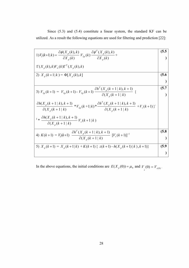
Since (5.3) and (5.4) constitute a linear system, the standard KF can be
utilized. As a result the following equations are used for filtering and prediction [22]:
1) 1(~ +kVx | =)k)(
)),((kX
kkX
p
p
∂
∂φ)(~ kV px )(
)),((kX
kkX
p
pT
∂
∂φ+
)),(()()),(( kkXkVkkX pwpΤΓΓ
(5.5
)
2) 1( +kX p | k ) = ]),([ kkX pΦ (5.6
)
3) )1(~ +kV px = )1(~ +kV px - )1(~ +kV px )|1(()1),|1((
kkXkkkXh
p
pT
+∂
++∂ {
)|1(()1),|1((
kkXkkkXh
p
p
+∂
++∂ * kV px (~ +1| )k *
)|1(()1),|1((
kkXkkkXh
p
pT
+∂
++∂ + )1( +kVv }-
1 * )|1((
)1),|1((kkXkkkXh
p
p
+∂
++∂1( +kVx | k )
(5.7
)
4) )1( +kK = 1(~ +kVx ) )|1((
)1),|1((kkXkkkXh
p
pT
+∂
++∂ 1)]1([ −+kVv
(5.8
)
5) )1( +kX p = 1( +kX p | )k + )1( +kK { )1( +kz – )1(( +kXh p | k ) )}1, +k (5.9
)
In the above equations, the initial conditions are 0))0(( µ=pXE and )0()0(~ xx
VV = .
29
CHAPTER 6
APPLICATION OF EKF TO ECONOMETRICS
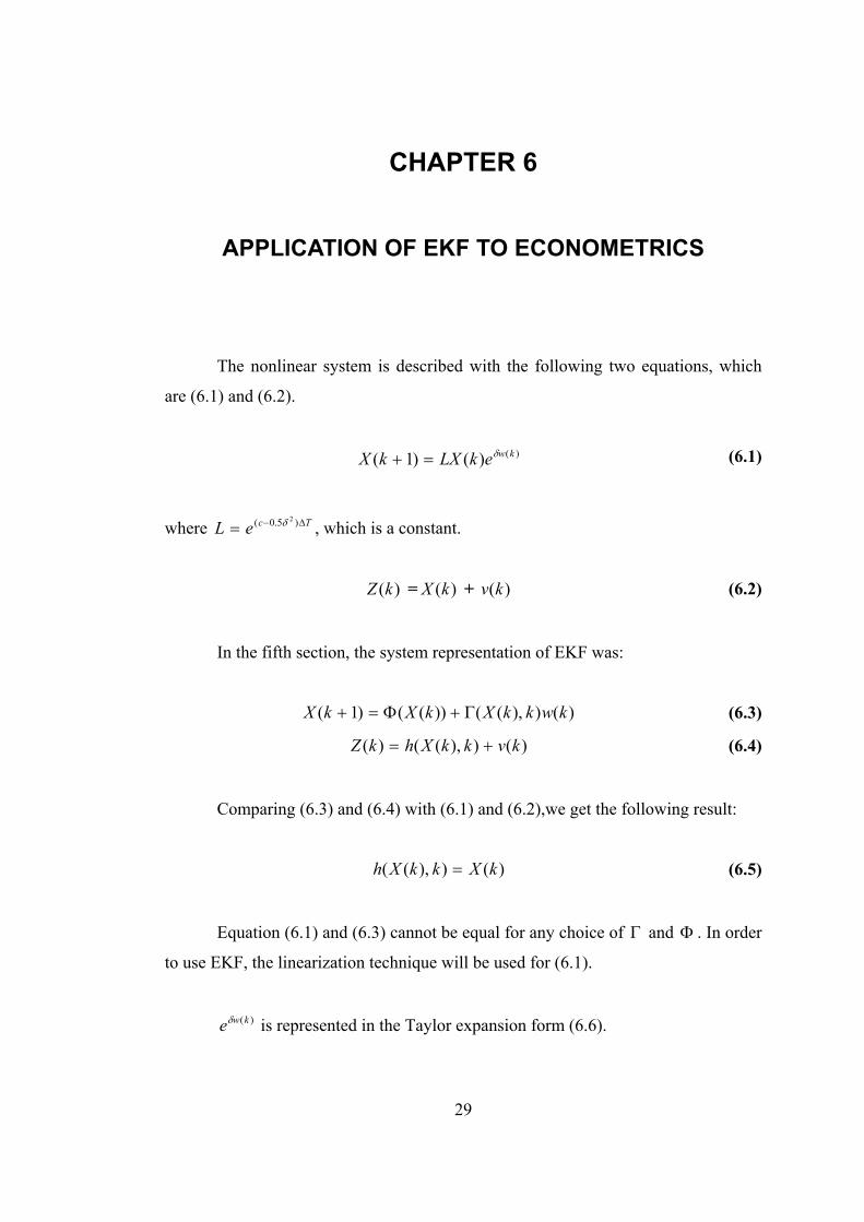
The nonlinear system is described with the following two equations, which
are (6.1) and (6.2).
)()()1( kwekLXkX δ=+ (6.1)
where TceL ∆−= )5.0( 2δ , which is a constant.
)(kZ = )(kX + )(kv (6.2)
In the fifth section, the system representation of EKF was:
)()),(())(()1( kwkkXkXkX Γ+Φ=+ (6.3)
)()),(()( kvkkXhkZ += (6.4)
Comparing (6.3) and (6.4) with (6.1) and (6.2),we get the following result:
)()),(( kXkkXh = (6.5)
Equation (6.1) and (6.3) cannot be equal for any choice of Γ and Φ . In order
to use EKF, the linearization technique will be used for (6.1).
)(kweδ is represented in the Taylor expansion form (6.6).
30
...2
)]([)(12
)( +++=kwkwe kw δδδ
(6.6)
...]2
)]([)(1)[()(2
)( +++=∆ kwkwkLXekLX Tw δδδ
...)()()()( )( ++= kwkLXkLXekLX kw δδ …
Equation (6.7) is obtained by taking a first order approximation for Taylor
series
≈∆ )()( TwekLX δ )(kLX + )( TwL ∆δ )(kX (6.7)
Instead (6.1), equation (6.7) is used to be able to apply EKF. Comparing (6.7)
with (6.3), equations (6.8) and (6.9) are obtained.
=Φ )),(( kkX )(kLX (6.8)
=Γ )),(( kkX )(kXLδ (6.9)
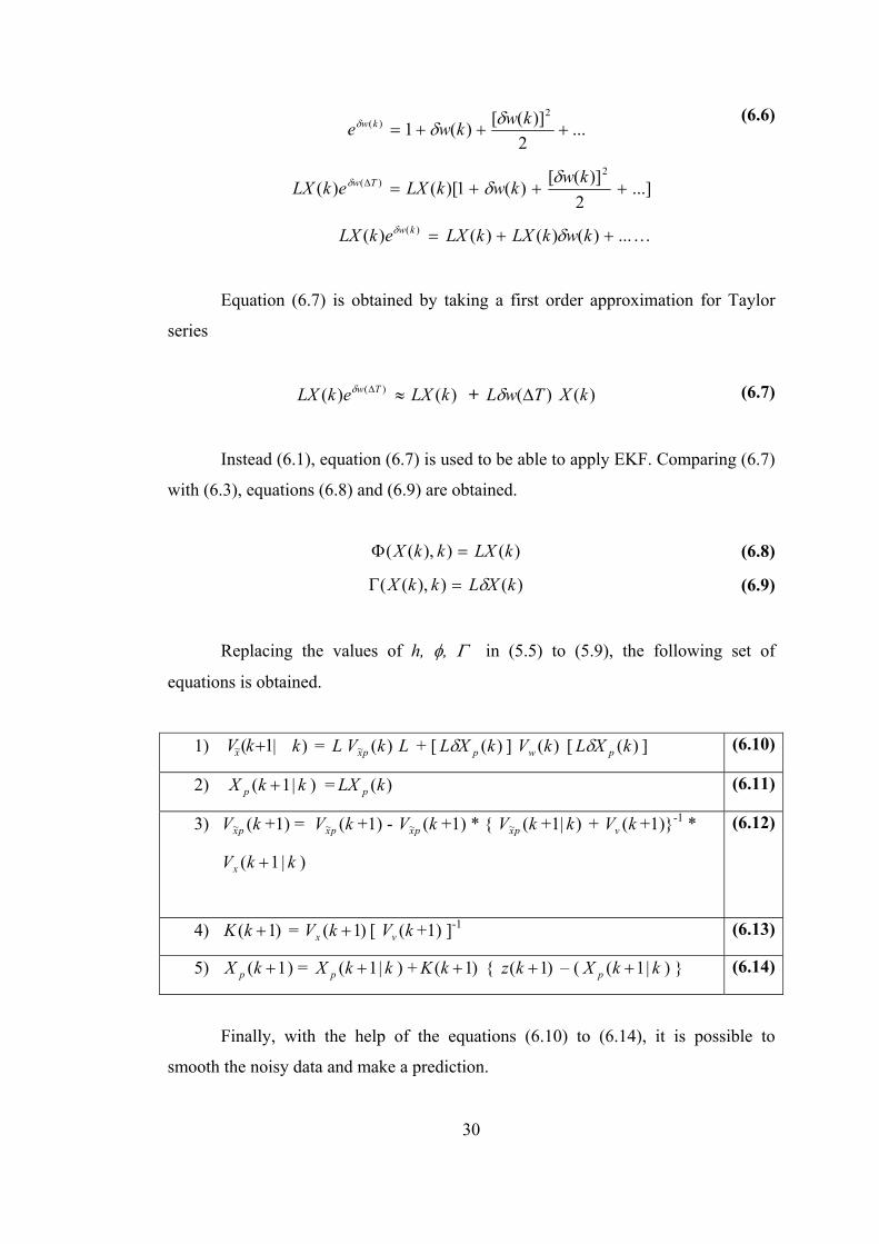
Replacing the values of h, φ, Γ in (5.5) to (5.9), the following set of
equations is obtained.
1) 1(~ +kVx | )k = L )(~ kV px L + [ )(kXL pδ ] )(kVw [ )(kXL pδ ] (6.10)
2) 1( +kX p | k ) = )(kLX p (6.11)
3) kV px (~ +1) = kV px (~ +1) - kV px (~ +1) * { kV px (~ +1| )k + kVv ( +1)}-1 *
1( +kVx | k )
(6.12)
4) )1( +kK = )1( +kVx [ kVv ( +1) ]-1 (6.13)
5) 1( +kX p ) = 1( +kX p | k ) + )1( +kK { )1( +kz – ( 1( +kX p | k ) } (6.14)
Finally, with the help of the equations (6.10) to (6.14), it is possible to
smooth the noisy data and make a prediction.
31
CHAPTER 7
PARTICLE FILTERS-SIR ALGORITHM
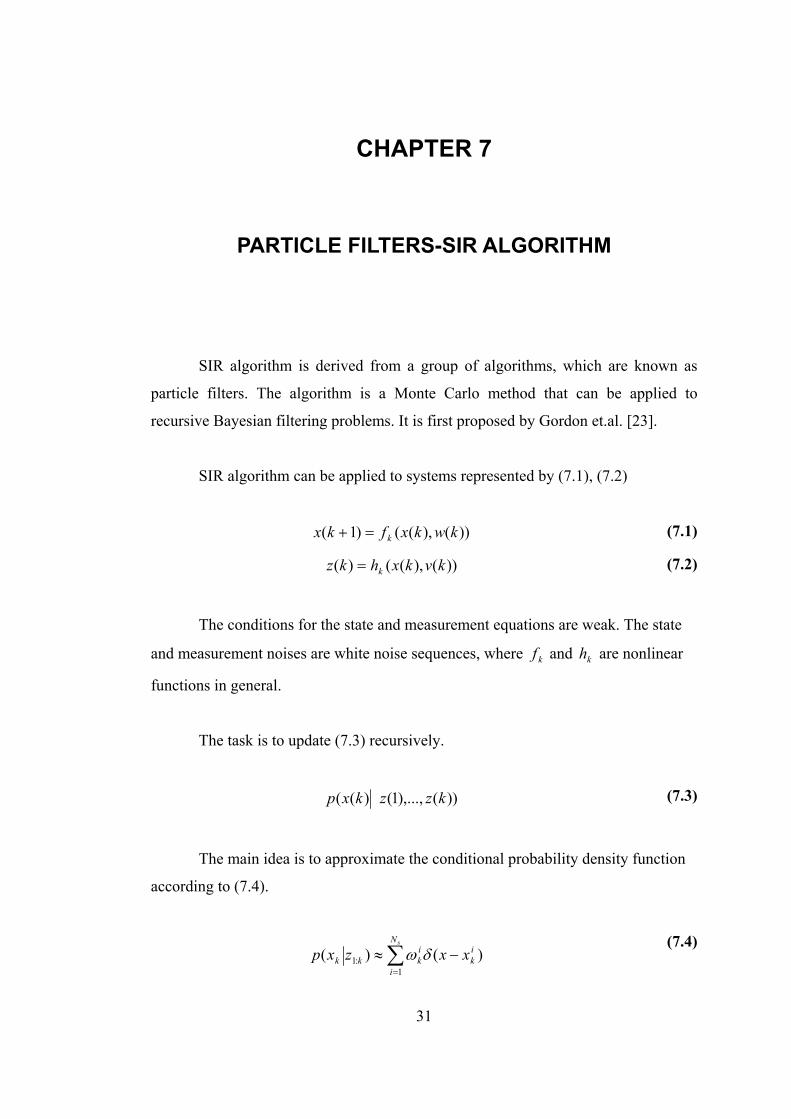
SIR algorithm is derived from a group of algorithms, which are known as
particle filters. The algorithm is a Monte Carlo method that can be applied to
recursive Bayesian filtering problems. It is first proposed by Gordon et.al. [23].
SIR algorithm can be applied to systems represented by (7.1), (7.2)
))(),(()1( kwkxfkx k=+ (7.1)
))(),(()( kvkxhkz k= (7.2)
The conditions for the state and measurement equations are weak. The state
and measurement noises are white noise sequences, where kf and kh are nonlinear
functions in general.
The task is to update (7.3) recursively.
))(),...,1()(( kzzkxp (7.3)
The main idea is to approximate the conditional probability density function
according to (7.4).
∑=
−≈sN
i
ik
ikkk xxzxp
1:1 )()( δω
(7.4)
32
Here, ikx represents the randomly generated particles and i
kw ’s are the
associated probability values. )(xδ is the usual impulse function. kz :1 denotes the set
{ })(),...,2(),1( kzzz . Also kx :1 denotes the set { })(),...,2(),1( kxxx .
The SIR filter is composed of three steps:
1) Prediction
2) Update
3) Resampling
Prediction
At the prediction step, given, )( 1:11 −− kk zxp the task is to obtain )( 1:1 −kk zxp
Each particle will be updated using the following equation (7.5).
))(),(()( 111 iwixfix kkkk −−−= (7.5)
Each )(1 iwk− is drawn from the probability density function (pdf) of )( 1−kwp .
Update
The weights of )(ixk in (7.4) are calculated according to (7.6).
∑=
=sN
jkk
kkk
jxzp
ixzpiw
1))((
))(()(
(7.6)

33
Resampling
When the update is completed, )( :1 kk zxp from )( 1:11 −− kk zxp is achieved. The
particles ikx and the associated probability values i
kw represent the conditional value
in the sense of (7.4). If the resampling step was to be skipped, then ikw would
become more and more skewed. After a while, only one particle with nonzero
probability value will exist [25]. To avoid this degeneracy, the resampling step is
proposed. As a result, the new pdf is represented by (7.7).
∑=
−=N
i
ik
itkk xxN
Nzxp
1:1 )(1)( δ
(7.7)
where
NNN
i
it =∑
=1
(7.8)
For more information about the resampling stage, the reader is referred to [24].
7.1 Derivation of the SIS and SIR algorithm
The sequential importance sampling (SIS) algorithm is a Monte Carlo (MC)
method that forms the basis for most sequential MC filters developed over the past
decades. SIR is also one of these filters.
Suppose )()( xxp π∝ , is a probability density function from which it is
difficult to draw samples, but for which )(xπ can be evaluated [as well as up to
proportionality]. In addition, let si Nixqx ,..,1),(~ = be samples that are easily
generated from a proposal )(xq called importance density. Then, a weighted
approximation to the density )(xp is given by
∑=
−≈sN
i
ii xxwxp1
)()( δ (7.9)
34
where
)()(
i
ii
xqxw π
∝ (7.10)
(7.10) is the normalized weight of the i ’th particle [24].
If the samples are drawn from )( :1:0 kk zxq , then the weights will be (7.11).
)()(
:1:0
:1:0
ki
k
ki
kik zxq
zxpw ∝
(7.11)
Let the importance density be chosen as:
)(),()( 1:11:0:11:0:1:0 −−−= kkkkkkk zxqzxxqzxq (7.12)
Using the Bayes rule:
)()(),(
)(1:1
1:1:01:1:0:1:0
−
−−=kk
kkkkkkk zzp
zxpzxzpzxp
(7.13)
)()(),(),(
)(1:1
1:11:01:11:01:1:0:1:0
−
−−−−−=kk
kkkkkkkkkk zzp
zxpzxxpzxzpzxp
(7.14)
Since the state is actually a Markov process (due to whiteness of the process
noise)
)(),( 11:11:0 −−− = kkkkk xxpzxxp (7.15)
35
and since the measurements are a static function of the last state and the
measurement noise is white
)(),( 1:1:0 kkkkk xzpzxzp =− (7.16)
)()()()(
)(1:1
1:11:01:1:0
−
−−−=kk
kkkkkkkk zzp
zxpxxpxzpzxp
(7.17)
)()()()( 1:11:01:1:0 −−−∝ kkkkkkkk zxpxxpxzpzxp (7.18)
Putting (7.12) and (7.18) into (7.11), the resulting equations (7.19) and (7.20)
are obtained.
)(),(
)()()(
1:11:0:11:0
1:11:01
−−−
−−−∝
ki
kki
kik
ki
kik
ik
i
kkik zxqzxxq
zxpxxpxzpw
(7.19)
),(
)()(
:11:0
11
ki
kik
ik
ik
i
kkik
ik zxxq
xxpxzpww
−
−−∝
(7.20)
Hence, the general framework for SIS filters is concluded.
The SIR filter is easily derived by choosing
)(),( 1:11:0ikkk
ikk xxpzxxq −− = (7.21)
Then,
)(1i
kkik
ik xzpww −∝ (7.22)

36
Hence the weights are updated according to the (7.22) and ix ’s are updated
according to the (7.21).

37
CHAPTER 8
SIMULATIONS OF FILTERING AND PREDICTION EXPERIMENTS
8.1 General Outline
In this section, the econometric system is analyzed from several aspects.
The system was described by (8.1) and (8.2).
)()()1( kwekLXkX δ=+ (8.1)
where TceL ∆−= )5.0( 2δ , which is a constant. (8.1) is the standard state equation. In real
world applications, it corresponds to the real price update in terms of current real
price and noise.
The observation equation is defined by (8.2).
)(kZ = )(kX + )(kv (8.2)
where )(kv is the measurement noise or speculators noise or, alternatively, the
traders noise. (8.1) and (8.2) constitute together the dynamic system representation.
In this section, it is assumed that the measurement data is given and the task
is to filter the noise and expect the current and the next real price
38
8.2 Filtering Tools
The previous literature on filtering generally views the Extended Kalman
Filter as a, standard analysis tool for filtering of noise for nonlinear dynamic
systems. In this study, an alternative method DQF, as mentioned before in details, is
used. Although the theory of DQF is discussed in section 4.1, the applications of
DQF to several cases need to be worked out. Therefore, this study is an attempt to
apply DQF to a new area, Mathematical Finance, which became increasingly popular
in the recent years.
8.3 Prediction Tools
Needless to mention, prediction is crucially important in economic systems.
In this context, predicting the most probable next value of the stock emerges as an
interesting question to answer. In order to predict the next value of the stock, which
is described by the system representation (8.1) and (8.2), SIR filter and EKF are
used.
8.4 Error Criteria and Monte Carlo Simulations
When there is great deal of difficulty in analyzing the systems in several
branches of science, Monte Carlo simulations are employed. Therefore, in this study,
to compare the performances of EKF and DQF, this method is preferred. The method
can simply be summarized as making many experiments and using the results of
these experiments to predict the performance of the system.
In each simulation experiment, the followed procedure is similar:
1) One parameter is varied (or chosen a specific value).
2) For each value of the parameter, 20 experiments are done.
3) Errors for each experiment are calculated for
o EKF output
39
o DQF output
4) Average Error EKF and DQF are calculated.
8.4.1 Filtering Error
8.4.1.1 Error in RN Spaces:
Let NRx ∈ be defined by (8.3).
)](),...,2(),1([ Nxxxx = (8.3)
2L norm of x is calculated according to (8.4)
2
12 )]([∑
=
=N
iixx
(8.4)
Let NRyx ∈, , then the distance between the vectors x and y is given by
(8.6)
2yx − (8.6)
The distance concept defined in (8.6) is used for the definition of error. Let x
be the “true” value then the yerror is defined by (8.7)
2yxerrory −= (8.7)
8.4.1.2 Errors in the Experiments
In order to calculate the errors, the notations (8.8) to (8.11) are used to
represent real data, EKF output, and DQF output respectively.
40
[=X )1(X , )2(X , … , )](NX (8.8)
)1([EKFEKF = , )2(EKF , … , )](NEKF (8.10)
)1([DQFDQF = , )2(DQF , … , )](NDQF (8.11)
The corresponding error values of EKF and DQF are calculated according to
(8.12) and (8.13)
2XEKFerrorEKF −=2
1)]()([∑
=
−=N
iiXiEKF
(8.12)
2XDQFerrorDQF −=2
1)]()([∑
=
−=N
iiXiDQF
(8.13)
Having obtained the errors for each experiment, the average of the errors of
both EKF and DQF are calculated according to the following formula in (8.14).
erroraverage _ = ∑=
K
i
ierrorK 1
)(1 (8.14)
where K is the number of experiments done in the Monte Carlo simulation.
8.4.2 Prediction Error
For a single experiment, the error calculations of prediction algorithms of
interest, which are EKF and SIR particle filter, are (8.15) and (8.16).
)1()1( +−+= NXNEKFerrorEKF (8.15)
)1()1( +−+= NXNSIRerrorSIR (8.16)
Having obtained the errors for each experiment, then the average of the errors
of both EKF and SIR particle filter are calculated according to the formula (8.17).
41
erroraverage _ = ∑=
K
i
ierrorK 1
)(1 (8.17)
where K is the number of experiments done in one Monte Carlo simulation.
8.5 Simulations
After the simulation results are obtained, the following regularities have been
observed:
1) The principle of EKF algorithm is the linearization of the system equations.
When the linearization condition is violated, the error performance of EKF
becomes poor.
2) In order to obtain good error performance for DQF algorithm, the
quantization levels must be adequately chosen. When this condition is
satisfied, DQF performs better compared to EKF.
3) The computation time performance of the DQF algorithm is bad when it is
compared to EKF.
Quantization Level
As implied above and the results show, the DQF algorithm has exponential
complexity, which stands out as its biggest disadvantage. It is hard to implement it in
real time applications, where the computation time performance is the crucial point.
In econometrics, there are several cases where the computation time is not the
primary concern. Therefore, if the space must is adequately quantized, then the DQF
algorithm may be preferred. However, the state equation (8.1) contains an
exponential term (8.18)
)(keδω (8.18)
With the term (8.18), it is more difficult to adequately describe the system in
the quantized domain. It requires a huge number of quantization level.
42
Linearization Condition
(8.18) is expressed in Taylor expansion form as (8.19).
)(kweδ = 1 + )(kwδ + 2
)]([2kwδ ] + …
(8.19)
Then, a first order approximation (8.20) has been made.
≈)(kweδ 1 + )(kwδ (8.20)
In order (8.20) to be an adequate approximation of (8.19), (8.21) must be
satisfied.
)()]([ 2 kwkw δδ << (8.21)
(8.21) is also equivalent to (8.22).
1)( <<kwδ (8.22)
43
8.5.1 Filtering
8.5.1.1
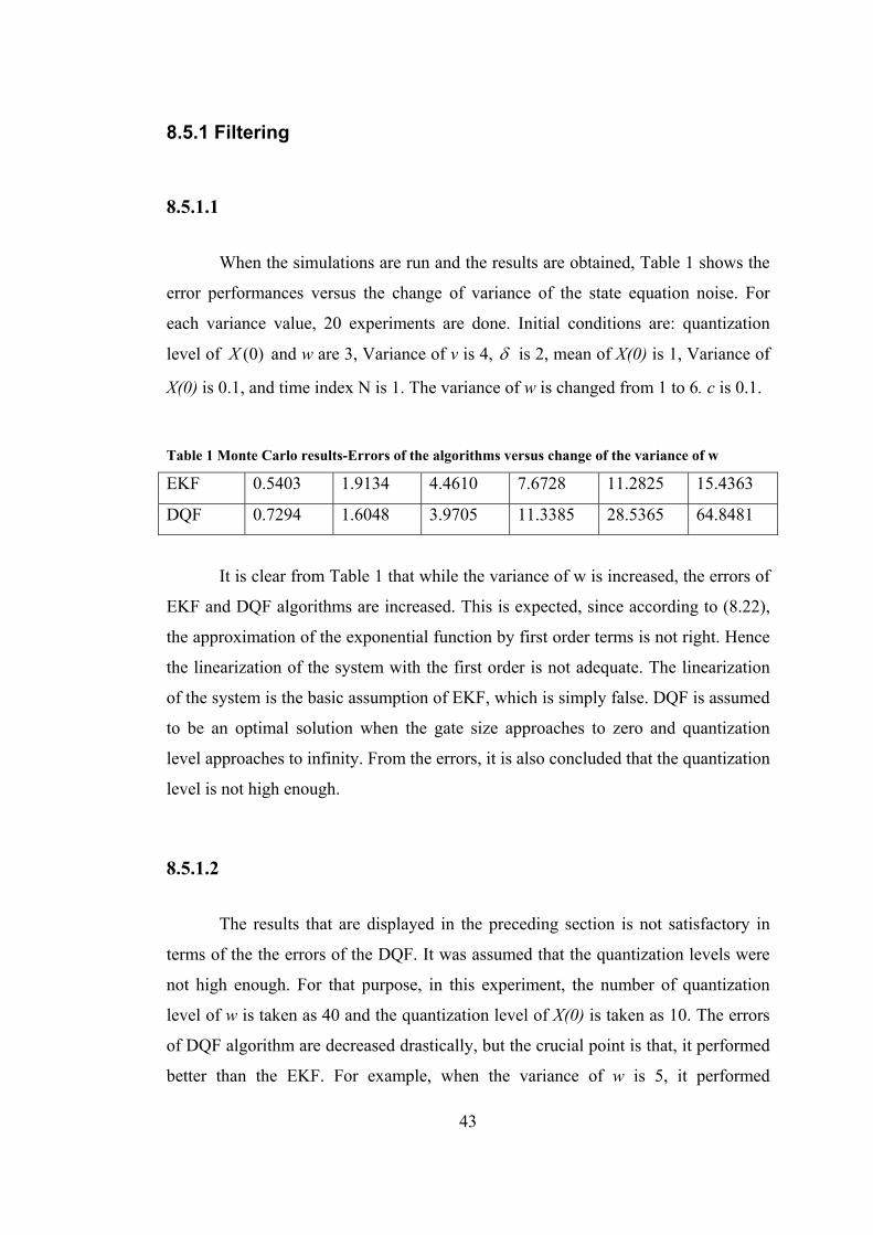
When the simulations are run and the results are obtained, Table 1 shows the
error performances versus the change of variance of the state equation noise. For
each variance value, 20 experiments are done. Initial conditions are: quantization
level of )0(X and w are 3, Variance of v is 4, δ is 2, mean of X(0) is 1, Variance of
X(0) is 0.1, and time index N is 1. The variance of w is changed from 1 to 6. c is 0.1.
Table 1 Monte Carlo results-Errors of the algorithms versus change of the variance of w
EKF 0.5403 1.9134 4.4610 7.6728 11.2825 15.4363
DQF 0.7294 1.6048 3.9705 11.3385 28.5365 64.8481
It is clear from Table 1 that while the variance of w is increased, the errors of
EKF and DQF algorithms are increased. This is expected, since according to (8.22),
the approximation of the exponential function by first order terms is not right. Hence
the linearization of the system with the first order is not adequate. The linearization
of the system is the basic assumption of EKF, which is simply false. DQF is assumed
to be an optimal solution when the gate size approaches to zero and quantization
level approaches to infinity. From the errors, it is also concluded that the quantization
level is not high enough.
8.5.1.2
The results that are displayed in the preceding section is not satisfactory in
terms of the the errors of the DQF. It was assumed that the quantization levels were
not high enough. For that purpose, in this experiment, the number of quantization
level of w is taken as 40 and the quantization level of X(0) is taken as 10. The errors
of DQF algorithm are decreased drastically, but the crucial point is that, it performed
better than the EKF. For example, when the variance of w is 5, it performed
44
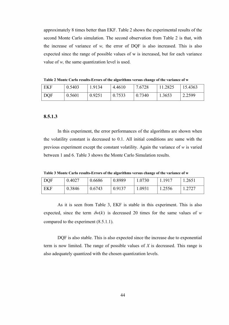
approximately 8 times better than EKF. Table 2 shows the experimental results of the
second Monte Carlo simulation. The second observation from Table 2 is that, with
the increase of variance of w, the error of DQF is also increased. This is also
expected since the range of possible values of w is increased, but for each variance
value of w, the same quantization level is used.
Table 2 Monte Carlo results-Errors of the algorithms versus change of the variance of w
EKF 0.5403 1.9134 4.4610 7.6728 11.2825 15.4363
DQF 0.5601 0.9251 0.7533 0.7340 1.3653 2.2599
8.5.1.3
In this experiment, the error performances of the algorithms are shown when
the volatility constant is decreased to 0.1. All initial conditions are same with the
previous experiment except the constant volatility. Again the variance of w is varied
between 1 and 6. Table 3 shows the Monte Carlo Simulation results.
Table 3 Monte Carlo results-Errors of the algorithms versus change of the variance of w
DQF 0.4027 0.6686 0.8989 1.0730 1.1917 1.2651
EKF 0.3846 0.6743 0.9137 1.0931 1.2556 1.2727
As it is seen from Table 3, EKF is stable in this experiment. This is also
expected, since the term )(kwδ is decreased 20 times for the same values of w
compared to the experiment (8.5.1.1).
DQF is also stable. This is also expected since the increase due to exponential
term is now limited. The range of possible values of X is decreased. This range is
also adequately quantized with the chosen quantization levels.
45
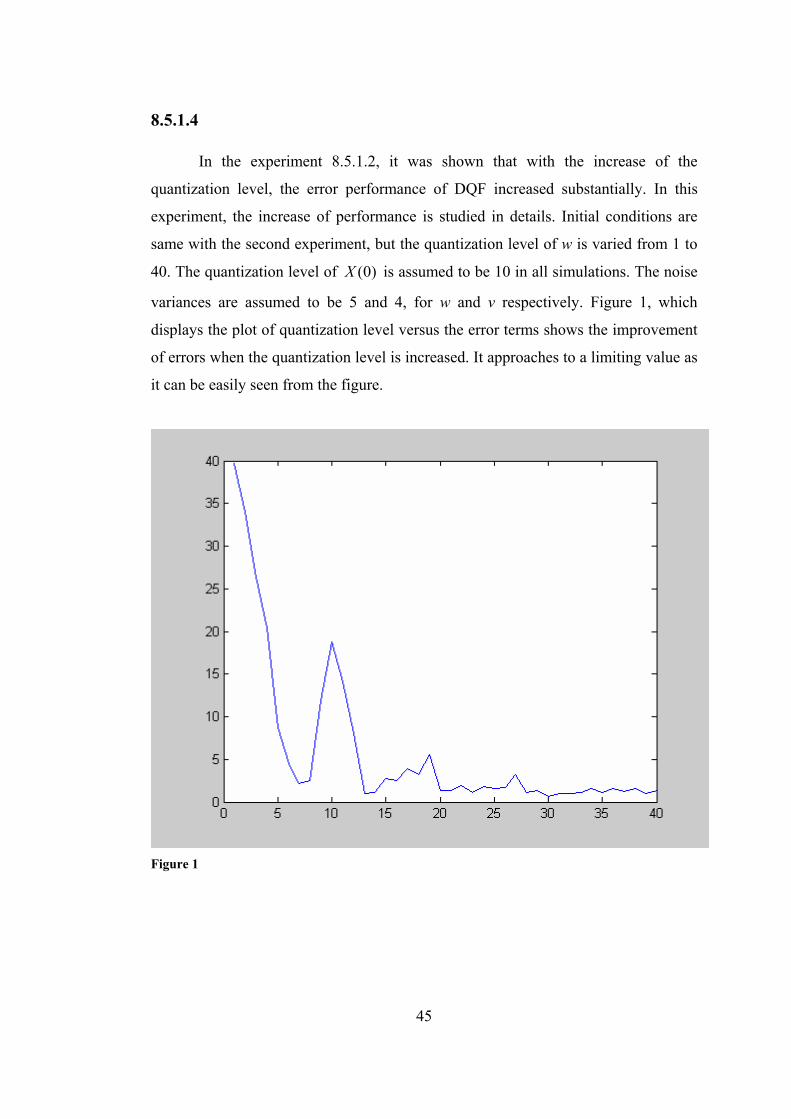
8.5.1.4
In the experiment 8.5.1.2, it was shown that with the increase of the
quantization level, the error performance of DQF increased substantially. In this
experiment, the increase of performance is studied in details. Initial conditions are
same with the second experiment, but the quantization level of w is varied from 1 to
40. The quantization level of )0(X is assumed to be 10 in all simulations. The noise
variances are assumed to be 5 and 4, for w and v respectively. Figure 1, which
displays the plot of quantization level versus the error terms shows the improvement
of errors when the quantization level is increased. It approaches to a limiting value as
it can be easily seen from the figure.
Figure 1
46
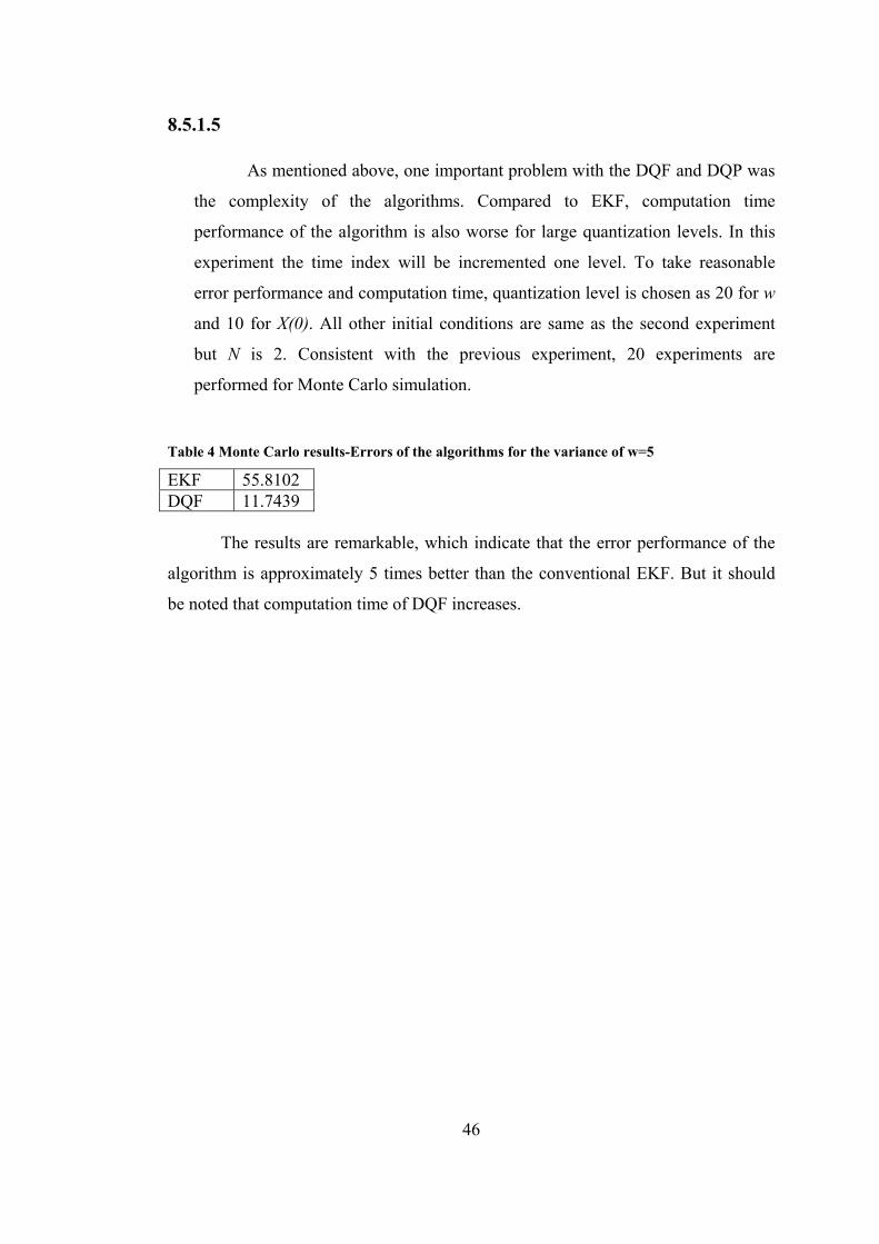
8.5.1.5
As mentioned above, one important problem with the DQF and DQP was
the complexity of the algorithms. Compared to EKF, computation time
performance of the algorithm is also worse for large quantization levels. In this
experiment the time index will be incremented one level. To take reasonable
error performance and computation time, quantization level is chosen as 20 for w
and 10 for X(0). All other initial conditions are same as the second experiment
but N is 2. Consistent with the previous experiment, 20 experiments are
performed for Monte Carlo simulation.
Table 4 Monte Carlo results-Errors of the algorithms for the variance of w=5
EKF 55.8102 DQF 11.7439
The results are remarkable, which indicate that the error performance of the
algorithm is approximately 5 times better than the conventional EKF. But it should
be noted that computation time of DQF increases.
47
8.5.2 Prediction
The prediction part differs from the smoothing part. The system described by
(8.23) and (8.24) is transformed to another equivalent form. The reason for that is the
number of experiments in the Monte Carlo simulation required to compare DQP and
EKF is too high. However, after transforming to the new equivalent form, better
results have been obtained. Furthermore, the time index could be incremented to
even higher numbers, which was not possible before for the case of DQF algorithm.
)()()1( kwekLXkX δ=+ (8.23)
)()()( kvkXkZ += (8.24)
When taking logarithm of both sides, (8.23) is rewritten as (8.25)
)())(ln()ln())1(ln( kwkxLkX δ++=+ (8.25)
Furthermore if
))(ln()( kXkY = (8.26)
)()()ln()1( kwkYLkY δ++=+ (8.27)
As a result the new set of equations are (8.27) and (8.28).
)()( )( kvekZ kY += (8.28)
The equation (7.27) is linear, but the equation (7.28) is nonlinear.
Furthermore the probability density function of )0(Y is not Gaussian. In fact, it is
obtained from the Gaussian noise by the transformation (8.26). Hence the standard
assumption of EKF for the initial noise does not hold.Even in this case, the new set
of nonlinear equation is implemented by SIR and EKF algorithm.
48
Mean and Variance of Y(0)
)(kY can take values 0 and negative, so )0(Y can have complex values
according to (8.26). For that reason, all the values for 0)( ≤kY is approximated by
001.0)( =kY . This makes sense, since the mean of )0(X is 1 and its variance is
taken as 0.1. Under these assumptions, mean and variance of )0(Y is obtained
experimentally. For that purpose (8.29) and (8.30) are used.
N
YN
ii
Y
∑== 1
)0(µ
(8.29)
1
)(1
2)0(
2)0( −
−=∑=
N
Ys
N
iYi
Y
µ
(8.30)
where iY is the randomly generated number. These estimates are known to converge
to the true mean and variance values as ∞→N .
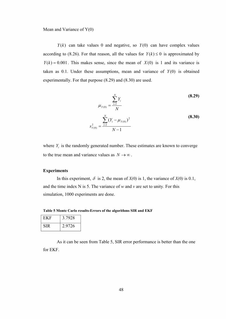
Experiments
In this experiment, δ is 2, the mean of X(0) is 1, the variance of X(0) is 0.1,
and the time index N is 5. The variance of w and v are set to unity. For this
simulation, 1000 experiments are done.
Table 5 Monte Carlo results-Errors of the algorithms SIR and EKF
EKF 3.7928
SIR 2.9726
As it can be seen from Table 5, SIR error performance is better than the one
for EKF.
49
CHAPTER 9
SIMULATIONS OF FILTERING EXPERIMENTS FOR STOCHASTIC GROWTH MODELS
Beginning with the standard stochastic growth models, for which the typical
solutions are offered in Hansen [27],[28], modeling both productivity shocks and
capital stock accumulation became critical issues. Although, the relationship between
the two variables can be explained in a standard way by using the “Solow residuals”,
there are also some recent studies, which explain the dynamics within the context of
more compact models. However, there are only a few of these studies that attempt to
explore the issue in a non-linear framework. However, as it is evidently discussed in
Novales et al [29], the productivity shocks may carry a non-linear nature, for which
the standard Kalman filtering algorithms fail to be appropriate. In this context, the
non-linear state space model can be solved either by extended Kalman filter or
Particle filter. Following Novales et al [29], the state space model can be written as:
)())1(log())(log( ttt εθρθ +−= (9.1)
)()()( tNtctk ++= αθ (9.2)
The first equation (9.1) models the productivity shocks as being first order
autoregressive process, where the disturbance term is assumed to be independent and
identically distributed. If the parameter rho gets closer to unity, then the productivity
shocks follow random walk processes, where any shock to the equation will have
permanent effects.
The second equation (9.2) relates the importance of these productivity shocks
on the change of the capital stock. Based on the neo-classical growth models, an
increase in the productivity will increase the return to the capital, which will create
50
an extra incentive for the firms to accumulate further capital. Using the parameters
that are obtained from the calibration of the micro-based fundamentals, the following
values for the parameters are used.
73.0=c (9.3)
75.1=α (9.4)
1=ρ (9.5)
In terms of estimation, the first equation, which is the state equation in the
model, has a non-linear nature, where the performance of extended Kalman filter and
Particle filter can be tested.
By use of the transformation (9.6), the equations (9.7) and (9.8) are obtained.
))(ln()( ttX θ= (9.6)
)()1()( ttXtX ε+−= (9.7)
)()( )( tNectk tX ++= α (9.8)
The mean and variance are calculated experimentally.
Mean and Variance of X(0)
As before, )0(θ can take values 0 and negative, so )0(X can have complex
values according to (9.6). For that reason, all the values for 0)0( ≤θ is approximated
by 001.0)0( =θ . This makes sense, since the mean of )0(θ is 1 and its variance is
taken as 0.1. Under these assumptions, the mean and the variance of )0(X is
obtained experimentally.
N
XN
ii
X
∑== 1
)0(µ
(9.9)

51
1
)(1
2)0(
2)0( −
−=∑=
N
Xs
N
iXi
X
µ
(9.10)
where iX is the randomly generated number. These estimates are known to
converge to the true mean and variance values as ∞→N .
Experiment
In this experiment, filtering performance of the algorithms of SIR and EKF
are compared. Mean of X(0) is 1, variance of X(0) is 0.1, and the time index N is 5.
The variance of w is 1. The variance of v is 1. For this simulation, again, 1000
experiments are done.
Table 6 Monte Carlo results-Errors of the algorithms SIR and EKF
EKF 2.0875
SIR 1.2836
As seen from Table 6, error performance of the SIR algorithm is better than
the EKF algorithm.
Therefore, the last two experiments clearly show that when the SIR algorithm
is compared with the conventionally used Extended Kalman Filter, it has better
performances. Such a conclusion indicates that SIR can be a competing alternative to
EKF in computation process of the econometrics problem.
52
CHAPTER 10
CONCLUSION
This study extends the previous work on the nonlinear estimation problems.
For that purpose, Extended Kalman Filter (EKF), Discrete Quantization Filter and
Sequential Importance Resampling (SIR) Filter are employed. . Since the already
dense literature on nonlinear estimation has not evaluated the last two filters, this
study can be viewed as a contribution in offering two alternative algorithms. Another
primary concern in this thesis is to show the advantages of these two algorithms over
EKF, which is the conventionally used algorithm in the field.
The main idea of DQF is to quantize the random variables. If sufficient
quantization of the random variables are made, then DQF performs better than the
EKF. However, its major disadvantage is the computation time. Hence there is a
trade-off for performance versus computation time.
SIR filter is from a group of filters that are known as particle filters. It is the
implementation of Monte Carlo techniques to estimation problems. Error
performances of the SIR filter were better compared to EKF. The computation time
performance was also reasonable compared to DQF. Therefore, the filter can be seen
as a good alternative to theEKF.
The case studies were chosen from the field of econometrics. Hence, the
control theory techniques have been applied to a different science branch.
Other than evaluating the performance of the above mentioned algorithms,
another primary concern in this study is to promote the use of stochastic calculus,
which enables us to have a more general perspective for nonlinear dynamical
systems with noise. The classical approach in the system theory is to make
assumptions for noise directly in the state space form. However, with the use of
stochastic calculus, we can make assumptions also in the differential equations form.

53
Although the theory behind this subject requires understanding advanced
mathematical concepts, its usage is fairly simple.
54
REFERENCES
[1] Mohinder S.Grewal and Angus P. Andrews, Kalman Filtering Theory and Practice using Matlab,John Wiley,New York, 2001
[2] C.K.Chui and G.Chen, Kalman Filtering with Real-Time Applications,
Springer, Berlin; New York, 1999
[3] Kerim Demirbaş, Information Theoretic Smoothing Algorithms for Dynamic Systems with or without Interference, Control and Dynamic Systems , pp.175-295
[4] Thomas Kailath, Linear Systems, Prentice Hall, Englewood Cliffs, N. J., 1980 [5] Zdzislaw Brzezniak and Tomasz Zastawniak, Basic Stochastic Processes,
Springer-Verlag, London Limited, 1999, pp.179-222 [6] Thomas Mikosch, Elementary Stochastic Calculus, World Scientific,
Singapore; River Edge, N. J., pp. 180, 1998 [7] Thomas Mikosch, Elementary Stochastic Calculus, World Scientific,
Singapore; River Edge, N. J., pp. 168, 1998 [8] Thomas Mikosch, Elementary Stochastic Calculus, World Scientific,
Singapore; River Edge, N. J., pp. 35, 1998
[9] Hayri Körezlioğlu, Azize Bastıyalı Hayfavi, Elements of Probability Theory, ODTÜ, Ankara, 2001
[10] Bernt Oksendal, Stochastic Differential Equations, An Introduction with
Applications, Springer, Berlin; New York, pp. 36, 1995
[11] Thomas Mikosch, Elementary Stochastic Calculus, World Scientific, Singapore; River Edge, N. J., pp. 93, 1998
[12] Ludwig Arnold, Stochastic Differential Equations Theory and Applications,
Wiley, New York, pp. 13, 1974
[13] Thomas Mikosch, Elementary Stochastic Calculus, World Scientific, Singapore; River Edge, N. J., pp. 101, 1998
[14] Thomas Mikosch, Elementary Stochastic Calculus, World Scientific,
Singapore; River Edge, N. J., pp. 190, 1998
55
[15] Thomas Mikosch, Elementary Stochastic Calculus, World Scientific, Singapore; River Edge, N. J., pp. 108-109, 1998
[16] Thomas Mikosch, Elementary Stochastic Calculus, World Scientific,
Singapore; River Edge, N. J., pp. 117, 1998
[17] Thomas Mikosch, Elementary Stochastic Calculus, World Scientific, Singapore; River Edge, N. J., pp. 118-119, 1998
[18] Thomas Mikosch, Elementary Stochastic Calculus, World Scientific,
Singapore; River Edge, N. J., pp. 138, 1998
[19] Thomas Mikosch, Elementary Stochastic Calculus, World Scientific, Singapore; River Edge, N. J., pp. 137, 1998
[20] Kerim Demirbaş, Information Theoretic Smoothing Algorithms for
Dynamic Systems with or without Interference, Control and Dynamic Systems , pp. 248
[21] Kerim Demirbaş, Information Theoretic Smoothing Algorithms for
Dynamic Systems with or without Interference, Control and Dynamic Systems , pp. 292
[22] A.P. Sage and J.L. Melsa, “Estimation Theory with Applications to
Communications and Control”, McGraw-Hill, New York, pp. 197
[23] N.Gordon, D. Salmond, and A.F.M. Smith, “Novel Approach to nonlinear and non-Gaussian Bayesian state estimation,” Proc. Inst. Elect. Eng., F, vol. 140, pp.107-113,1993
[24] M. Sanjeev Arulampalam, Simon Maskell, Neil Gordon, and Tim Clapp, A
Tutorial on Particle Filters for Online Nonlinear/Non-Gaussian Bayesian Tracking, IEEE Transactions On Signal Processing, Vol. 50, No. 2, February 2002
[25] Arnoud Doucet, Nando de Freitas, Neil Gordon, Sequential Monte Carlo
Methods in Practice, Springer-Verlag 2001, pp.10
[26] Kerim Demirbaş, Information Theoretic Smoothing Algorithms for Dynamic Systems with or without Interference, Control and Dynamic Systems , pp.292
[27] Hansen, G.D. (1985), "Indivisible Labor and The Business Cycle", Journal
of Monetary Economics, 16, 309-327.
[28] Hansen, G.D. (1997), "Technical Progress and Aggregate Fluctuations", Journal of Economic Dynamics and Control, 21, 1005-1023.

56
[29] Novales A., E. Dominguez, J.J. Perez and J. Ruiz (1999), "Solving Nonlinear Rational Expectations Models By Eigenvalue-Eigenvector Decompositions", in R. Marimon and A. Scott eds., Computational Methods For The Study Of Dynamic Economies, Oxford University Press, Oxford, UK.
57
APPENDIX Comma Seperated Form for the quantization of the Gaussian random variable upto 40 points. Quantized values for the random variable with mean 0 and variance 1. 1:0 2:-0.675,0675 3-1.0050,0,1.0050 4:.2190,-0.3550,0.3550,1.2190 5:.3760,-0.5920,0,0.5920,1.3760 6:-1.4990,-0.7670,-0.2420,0.2420,0.7670,1.4990 7:.5990,-0.9050,-0.4230,0,0.4230,0.9050,1.5990 8:-1.6830,-1.0180,-0.5670,-0.1830,0.1830,0.5670,1.0180,1.6830 9:-1.7581,-1.1173,-0.6884,-0.3310,-0.0001,0.3309,0.6882,1.1172,1.7580 10:-1.8221,-1.2005,-0.7900,-0.4534,-0.1482,0.1480,0.4532,0.7898,1.2003,1.8219 11:-1.8790,-1.2736,-0.8780,-0.5578,-0.2719,-0.0002,0.2716,0.5575,0.8778,1.2733, 1.8788 12:-1.9301,-1.3385,-0.9555,-0.6485,-0.3777,-0.1243,0.1239,0.3773,0.6481,0.9552, 1.3382,1.9299 13:-1.9765,-1.3969,-1.0245,-0.7285,-0.4699,-0.2308,-0.0002,0.2303,0.4694,0.7280, 1.0241,1.3966,1.9762 14:-2.0189,-1.4499,-1.0867,-0.8000,-0.5515,-0.3239,-0.1071,0.1065,0.3233,0.5509, 0.7994,1.0862,1.4495,2.0186 15:-2.0580,-1.4984,-1.1432,-0.8644,-0.6245,-0.4065,-0.2007,-0.0004,0.1999,0.4058, 0.6238,0.8638,1.1426,1.4978,2.0575 16:-2.0941,-1.5430,-1.1949,-0.9231,-0.6905,-0.4805,-0.2838,-0.0941,0.0933, 0.2829,0.4797,0.6897,0.9223,1.1942,1.5423,2.0935 17:-2.1277,-1.5842,-1.2425,-0.9768,-0.7506,-0.5475,-0.3585,-0.1776,-0.0005,0.1766, 0.3574,0.5465,0.7497,0.9759,1.2416,1.5834,2.1271 18:-2.1591,-1.6226,-1.2865,-1.0264,-0.8058,-0.6086,-0.4261,-0.2527,-0.0841, 0.0829,0.2515,0.4249,0.6075,0.8047,1.0253,1.2856,1.6217,2.1584 19:-2.1886,-1.6584,-1.3275,-1.0723,-0.8567,-0.6648,-0.4880,-0.3208,-0.1594,-0.0007, 0.1580,0.3194,0.4866,0.6634,0.8554,1.0711,1.3264,1.6573,2.1877 20:-2.2164,-1.6920,-1.3659,-1.1151,-0.9039,-0.7167,-0.5448,-0.3831,-0.2278,-0.0761, 0.0745,0.2262,0.3815,0.5432,0.7151,0.9024,1.1136,1.3645,1.6908,2.2153 21:-2.2426,-1.7236,-1.4018,-1.1551,-0.9479,-0.7648,-0.5974,-0.4405,-0.2905,-0.1447 ,-0.0010,0.1428,0.2886,0.4386,0.5956,0.7630,0.9462,1.1534,1.4003,1.7222,2.2413 22:-2.2674,-1.7534,-1.4356,-1.1926,-0.9891,-0.8098,-0.6463,-0.4936,-0.3482,-0.2076 ,-0.0696,0.0675,0.2054,0.3461,0.4915,0.6442,0.8077,0.9871,1.1907,1.4339,1.7518, 2.2660
58
23:-2.2909,-1.7817,-1.4675,-1.2279,-1.0277,-0.8518,-0.6919,-0.5430,-0.4017,-0.2656 ,-0.1326,-0.0012,0.1302,0.2631,0.3993,0.5406,0.6896,0.8496,1.0256,1.2258,1.4656 ,1.7799,2.2894 24:-2.3133,-1.8085,-1.4978,-1.2613,-1.0642,-0.8914,-0.7347,-0.5892,-0.4515,-0.3194,-0.1908,-0.0643,0.0615,0.1880,0.3166,0.4488,0.5865,0.7320,0.8888,1.0617,1.2589 ,1.4956,1.8065,2.3116 25:-2.3347,-1.8339,-1.5265,-1.2929,-1.0986,-0.9286,-0.7749,-0.6324,-0.4981,-0.3695 ,-0.2448,-0.1226,-0.0016,0.1194,0.2417,0.3664,0.4950,0.6295,0.7720,0.9258,1.0959 ,1.2903,1.5240,1.8318,2.3328 26:-2.3551,-1.8582,-1.5537,-1.3228,-1.1312,-0.9638,-0.8128,-0.6731,-0.5418,-0.4163 ,-0.2951,-0.1767,-0.0599,0.0564,0.1732,0.2917,0.4129,0.5384,0.6699,0.8096 ,0.9607,1.1282,1.3200,1.5511,1.8558,2.3530 27:-2.3747,-1.8814,-1.5797,-1.3514,-1.1622,-0.9972,-0.8486,-0.7116,-0.5829,-0.4603 ,-0.3422,-0.2272,-0.1141,-0.0019,0.1102,0.2233,0.3384,0.4565,0.5792,0.7079,0.8451 ,0.9938,1.1589,1.3482,1.5768,1.8788,2.3724 28:-2.3934,-1.9036,-1.6046,-1.3786,-1.1917,-1.0290,-0.8827,-0.7480,-0.6217,-0.5018 ,-0.3865,-0.2744,-0.1647,-0.0562,0.0519,0.1604,0.2702,0.3822,0.4976,0.6176,0.7439 ,0.8788,1.0252,1.1880,1.3752,1.6013,1.9007,2.3909 29:-2.4114,-1.9249,-1.6284,-1.4046,-1.2198,-1.0592,-0.9150,-0.7824,-0.6585,-0.5409 ,-0.4281,-0.3189,-0.2121,-0.1068,-0.0023,0.1022,0.2074,0.3143,0.4236,0.5364,0.6541 ,0.7781,0.9107,1.0551,1.2158,1.4008,1.6248,1.9217,2.4087 30:-2.4288,-1.9453,-1.6511,-1.4295,-1.2466,-1.0880,-0.9458,-0.8153,-0.6934,-0.5780 ,-0.4676,-0.3608,-0.2566,-0.1543,-0.0530,0.0479,0.1492,0.2516,0.3557,0.4626 ,0.5731,0.6886,0.8105,0.9412,1.0836,1.2424,1.4254,1.6473,1.9419,2.4258, 31:-2.4454,-1.9650,-1.6730,-1.4533,-1.2723,-1.1155,-0.9751,-0.8465,-0.7266,-0.6132 ,-0.5049,-0.4004,-0.2987,-0.1990,-0.1006,-0.0028,0.0950,0.1935,0.2932,0.3950 ,0.4996,0.6080,0.7214,0.8414,0.9702,1.1107,1.2677,1.4489,1.6689,1.9612,2.4422 32:-2.4615,-1.9838,-1.6940,-1.4762,-1.2970,-1.1419,-1.0032,-0.8763,-0.7582,-0.6467 ,-0.5404,-0.4379,-0.3385,-0.2411,-0.1453,-0.0503,0.0444,0.1394,0.2352,0.3326, 0.4321,0.5346,0.6411,0.7526,0.8709,0.9979,1.1367,1.2920,1.4714,1.6895,1.9798,2.4580 33:-2.4770,-2.0020,-1.7142,-1.4981,-1.3206,-1.1672,-1.0301,-0.9049,-0.7884,-0.6787 ,-0.5742,-0.4736,-0.3762,-0.2811,-0.1876,-0.0951,-0.0032,0.0887,0.1811,0.2746,0.3698

59
,0.4673,0.5679,0.6726,0.7824,0.8990,1.0244,1.1616,1.3153,1.4931,1.7094,1.9977,2.4732 34:-2.4920,-2.0196,-1.7337,-1.5193,-1.3434,-1.1914,-1.0559,-0.9322,-0.8173,-0.7092 ,-0.6064,-0.5076,-0.4120,-0.3189,-0.2276,-0.1375,-0.0481,0.0411,0.1305,0.2206 ,0.3120,0.4052,0.5009,0.5997,0.7027,0.8109,0.9259,1.0498,1.1855,1.3377,1.5139, 1.7286,2.0149,2.4880 35:-2.5065,-2.0365,-1.7524,-1.5397,-1.3652,-1.2148,-1.0807,-0.9584,-0.8450 ,-0.7384,-0.6371,-0.5400,-0.4462,-0.3549,-0.2655,-0.1775,-0.0904,-0.0037, 0.0830,0.1702,0.2582,0.3476,0.4390,0.5329,0.6301,0.7315,0.8382,0.9517,1.0742 ,1.2085,1.3592,1.5339,1.7470,2.0316,2.5022 36:-2.5205,-2.0529,-1.7706,-1.5593,-1.3863,-1.2372,-1.1045,-0.9836,-0.8716,-0.7664 ,-0.6666,-0.5710,-0.4788,-0.3892,-0.3016,-0.2156,-0.1305,-0.0461,0.0382,0.1226,0.2077 ,0.2938,0.3814,0.4711,0.5634,0.6591,0.7590,0.8643,0.9765,1.0976,1.2305,1.3799,1.5532 ,1.7648,2.0476,2.5160, 37:-2.5341,-2.0687,-1.7881,-1.5783,-1.4066,-1.2588,-1.1274,-1.0078,-0.8971,-0.7932 ,-0.6948,-0.6007,-0.5100,-0.4219,-0.3360,-0.2517,-0.1686,-0.0862,-0.0042,0.0778,0.1602, 0.2434,0.3277,0.4137,0.5018,0.5926,0.6869,0.7854,0.8894,1.0003,1.1201,1.2518,1.3998 ,1.5718,1.7820,2.0631,2.5292 38:-2.5472,-2.0841,-1.8050,-1.5966,-1.4262,-1.2797,-1.1494,-1.0311,-0.9216,-0.8190, -0.7219,-0.6291,-0.5398,-0.4533,-0.3689,-0.2863,-0.2049,-0.1244,-0.0444,0.0354,0.1154 ,0.1960,0.2774,0.3601,0.4445,0.5311,0.6205,0.7134,0.8107,0.9134,1.0231,1.1416,1.2721 1.4189,1.5897,1.7985,2.0781,2.5420 39:-2.5600,-2.0989,-1.8214,-1.6143,-1.4452,-1.2998,-1.1707,-1.0535,-0.9452,-0.8438, -0.7479,-0.6564,-0.5684,-0.4832,-0.4003,-0.3192,-0.2395,-0.1607,-0.0826 ,-0.0047,0.0731,0.1512,0.2300,0.3098,0.3910,0.4740,0.5593,0.6474,0.7390,0.8351, 0.9366,1.0451,1.1625,1.2919,1.4375,1.6070,1.8145,2.0926,2.5545 40: -2.5724,-2.1133,-1.8372,-1.6314,-1.4634,-1.3192,-1.1912,-1.0751, -0.9679,-0.8677,-0.7729,-0.6826,-0.5958,-0.5120,-0.4304,-0.3507,-0.2725, -0.1953,-0.1189,-0.0429,0.0329,0.1089,0.1853,0.2625,0.3408,0.4206,0.5022,0.5862, 0.6731,0.7636,0.8584,0.9589,1.0663,1.1826,1.3108,1.4554,1.6237,1.8300,2.1066, 2.5666 Comma Seperated Form for the quantization of the Gaussian random variable upto 40 points. Associated probabilty values for the quantized values for the random variable with mean 0 and variance 1.
60
1:1 2:0.5,0.5 3: 0.3150,0.3700,0.3150 4: 0.2230,0.2770,0.2770,0.2230 5: 0.1690,0.2160,0.2300,0.2160,0.1690 6: 0.1340,0.1750,0.1910,0.1910,0.1750,0.1340 7: 0.1100,0.1450,0.1620,0.1660,0.1620,0.1450,0.1100 8: 0.0930,0.1230,0.1390,0.1450,0.1450,0.1390,0.1230,0.0930 9: 0.0787,0.1064,0.1209,0.1285,0.1308,0.1285,0.1210,0.1064,0.0788 10: 0.0684,0.0931,0.1065,0.1142,0.1177,0.1177,0.1142,0.1066,0.0931,0.0685 11: 0.0602,0.0823,0.0948,0.1023,0.1064,0.1077,0.1064,0.1023,0.0948,0.0824,0.0603 12:0.0536,0.0735,0.0851,0.0923,0.0967,0.0987,0.0988,0.0967,0.0923,0.0851,0.0736,0.0536 13:0.0481,0.0662,0.0769,0.0838,0.0883,0.0908,0.0916,0.0908,0.0883,0.0839,0.0769, 0.0663,0.0481 14:0.0435,0.0601,0.0700,0.0766,0.0810,0.0837,0.0850,0.0850,0.0837,0.0810,0.0766, 0.0700,0.0601,0.0435 15:0.0396,0.0548,0.0641,0.0703,0.0746,0.0775,0.0791,0.0796,0.0791,0.0775,0.0747, 0.0704,0.0641,0.0549,0.0396 16:0.0363,0.0503,0.0590,0.0649,0.0691,0.0719,0.0738,0.0747,0.0747,0.0738,0.0720, 0.0691,0.0649,0.0590,0.0504,0.0363 17:0.0334,0.0464,0.0545,0.0601,0.0641,0.0670,0.0690,0.0701,0.0705,0.0701,0.0690, 0.0671,0.0642,0.0602,0.0546,0.0465,0.0334 18:0.0308,0.0430,0.0506,0.0559,0.0598,0.0626,0.0646,0.0659,0.0665,0.0665,0.0659, 0.0647,0.0627,0.0598,0.0560,0.0506,0.0431,0.0309 19:0.0286,0.0400,0.0471,0.0522,0.0559,0.0587,0.0607,0.0621,0.0629,0.0632,0.0629, 0.0621,0.0608,0.0587,0.0560,0.0522,0.0472,0.0401,0.0287 20:0.0267,0.0373,0.0440,0.0488,0.0524,0.0551,0.0572,0.0586,0.0595,0.0600,0.0600, 0.0596,0.0586,0.0572,0.0552,0.0525,0.0489,0.0441,0.0374,0.0267 21:0.0249,0.0349,0.0413,0.0458,0.0493,0.0519,0.0539,0.0554,0.0564,0.0571,0.0573, 0.0571,0.0565,0.0555,0.0540,0.0520,0.0494,0.0459,0.0414,0.0350,0.0250 22:0.0234,0.0328,0.0388,0.0431,0.0464,0.0490,0.0510,0.0525,0.0536,0.0543,0.0546, 0.0547,0.0543,0.0536,0.0526,0.0511,0.0491,0.0466,0.0433,0.0389,0.0329,0.0235 23:0.0220,0.0309,0.0366,0.0407,0.0439,0.0464,0.0483,0.0498,0.0509,0.0517,0.0522, 0.0523,0.0522,0.0518,0.0510,0.0499,0.0484,0.0465,0.0440,0.0408,0.0367,0.0310,0.0221 24:0.0207,0.0291,0.0345,0.0385,0.0415,0.0439,0.0459,0.0474,0.0485,0.0493,0.0499,
61
0.0502,0.0502,0.0499,0.0494,0.0486,0.0474,0.0460,0.0441,0.0417,0.0386,0.0347,0.0292,0.0208 25:0.0196,0.0275,0.0327,0.0365,0.0394,0.0417,0.0436,0.0451,0.0462,0.0471,0.0477, 0.0481,0.0482,0.0481,0.0478,0.0472,0.0463,0.0452,0.0437,0.0419,0.0396,0.0366,0.0328,0.0277,0.0197 26:0.0185,0.0261,0.0310,0.0346,0.0375,0.0397,0.0415,0.0430,0.0441,0.0450,0.0457, 0.0461,0.0464,0.0464,0.0462,0.0458,0.0451,0.0442,0.0431,0.0417,0.0398,0.0376,0.0348,0.0312,0.0262,0.0186 27:0.0176,0.0248,0.0295,0.0329,0.0357,0.0378,0.0396,0.0410,0.0422,0.0431,0.0438, 0.0443,0.0446,0.0447,0.0446,0.0443,0.0439,0.0432,0.0423,0.0412,0.0397,0.0380, 0.0358,0.0331,0.0296,0.0249,0.0177 28:0.0167,0.0236,0.0281,0.0314,0.0340,0.0361,0.0378,0.0392,0.0404,0.0413,0.0420, 0.0426,0.0429,0.0431,0.0431,0.0429,0.0426,0.0421,0.0414,0.0405,0.0394,0.0380,0.0363,0.0342,0.0316,0.0282,0.0237,0.0168 29:0.0159,0.0225,0.0267,0.0299,0.0325,0.0345,0.0362,0.0376,0.0387,0.0396,0.0404, 0.0409,0.0413,0.0416,0.0416,0.0416,0.0414,0.0410,0.0405,0.0397,0.0388,0.0377,0.0364,0.0347,0.0327,0.0301,0.0269,0.0226,0.0160 30:0.0152,0.0214,0.0255,0.0286,0.0310,0.0330,0.0347,0.0360,0.0371,0.0381,0.0388, 0.0394,0.0398,0.0401,0.0402,0.0403,0.0401,0.0399,0.0395,0.0389,0.0382,0.0373,0.0362,0.0348,0.0332,0.0312,0.0288,0.0257,0.0216,0.0153 31:0.0145,0.0205,0.0244,0.0274,0.0297,0.0316,0.0332,0.0346,0.0357,0.0366,0.0373, 0.0379,0.0384,0.0387,0.0389,0.0390,0.0389,0.0388,0.0385,0.0380,0.0375,0.0367,0.0358,0.0347,0.0334,0.0319,0.0299,0.0276,0.0246,0.0207,0.0146 32:0.0138,0.0196,0.0234,0.0262,0.0285,0.0304,0.0319,0.0332,0.0343,0.0352,0.0359, 0.0366,0.0370,0.0374,0.0376,0.0378,0.0378,0.0377,0.0375,0.0371,0.0367,0.0361,0.0354,0.0345,0.0334,0.0321,0.0306,0.0287,0.0265,0.0236,0.0198,0.0140 33:0.0132,0.0188,0.0224,0.0252,0.0274,0.0292,0.0307,0.0319,0.0330,0.0339,0.0346, 0.0353,0.0358,0.0361,0.0364,0.0366,0.0366,0.0366,0.0365,0.0362,0.0359,0.0354,0.0348,0.0341,0.0332,0.0321,0.0309,0.0294,0.0276,0.0254,0.0226,0.0190,0.0134 34:0.0127,0.0180,0.0215,0.0242,0.0263,0.0280,0.0295,0.0307,0.0318,0.0327,0.0334, 0.0340,0.0345,0.0349,0.0352,0.0354,0.0356,0.0356,0.0355,0.0353,0.0350,0.0347,0.0342,0.0336,0.0329,0.0320,0.0309,0.0297,0.0283,0.0265,0.0244,0.0218,0.0182,0.0128 35:0.0122,0.0173,0.0207,0.0232,0.0253,0.0270,0.0284,0.0296,0.0306,0.0315,0.0323, 0.0329,0.0334,0.0338,0.0341,0.0344,0.0345,0.0346,0.0345,0.0344,0.0342,0.0339,0.0335,0.0330,0.0324,0.0317,0.0309,0.0298,0.0286,0.0272,0.0255,0.0235,0.0209,0.0175,0.0123
62
36:0.0117,0.0166,0.0199,0.0224,0.0244,0.0260,0.0274,0.0286,0.0296,0.0304,0.0312, 0.0318,0.0323,0.0327,0.0331,0.0333,0.0335,0.0336,0.0336,0.0335,0.0334,0.0332,0.0329,0.0325,0.0320,0.0314,0.0306,0.0298,0.0288,0.0276,0.0263,0.0246,0.0226,0.0201,0.0169,0.0119 37:0.0113,0.0160,0.0192,0.0216,0.0235,0.0251,0.0264,0.0276,0.0286,0.0294,0.0301, 0.0308,0.0313,0.0317,0.0321,0.0323,0.0325,0.0327,0.0327,0.0327,0.0326,0.0324,0.0322,0.0318,0.0314,0.0309,0.0303,0.0296,0.0288,0.0278,0.0267,0.0253,0.0237,0.0218,0.0194,0.0162,0.0114 38:0.0109,0.0154,0.0185,0.0208,0.0227,0.0242,0.0255,0.0266,0.0276,0.0284,0.0292, 0.0298,0.0303,0.0307,0.0311,0.0314,0.0316,0.0318,0.0318,0.0318,0.0318,0.0317,0.0315,0.0312,0.0309,0.0305,0.0300,0.0294,0.0287,0.0278,0.0269,0.0258,0.0245,0.0229,0.0211,0.0187,0.0157,0.0110 39:0.0105,0.0149,0.0178,0.0201,0.0219,0.0234,0.0247,0.0257,0.0267,0.0275,0.0282, 0.0288,0.0294,0.0298,0.0302,0.0305,0.0307,0.0309,0.0310,0.0310,0.0310,0.0309,0.0308,0.0306,0.0303,0.0300,0.0296,0.0290,0.0285,0.0278,0.0270,0.0260,0.0249,0.0237,0.0222,0.0204,0.0181,0.0151,0.0106 40:0.0101,0.0144,0.0172,0.0194,0.0211,0.0226,0.0238,0.0249,0.0258,0.0266,0.0273, 0.0280,0.0285,0.0289,0.0293,0.0296,0.0299,0.0300,0.0302,0.0302,0.0303,0.0302,0.0301,0.0300,0.0297,0.0295,0.0291,0.0287,0.0282,0.0276,0.0269,0.0261,0.0252,0.0241,0.0229,0.0214,0.0197,0.0175,0.0146,0.0103
Top Related