


Languages
Pages
Legal


Nonequilibrium ultrafast
excited state
dynamics in DNA
Dissertation zur Erlangung
des Doktorgrades
an der Fakultat fur Mathematik,
Informatik und Naturwissenschaften
Fachbereich Physik
der Universitat Hamburg
vorgelegt von Martina Pola
Hamburg, 2016

2
3
Tag der Disputation: 23.09.2016
Gutachter der Dissertation:
Prof. Dr. Michael Thorwart
Prof. Dr. Arwen Pearson
Mitglieder der Prufungskommission:
Prof. Dr. Daniela Pfannkuche
Prof. Dr. Michael Thorwart
Prof. Dr. Arwen Pearson
Prof. Dr. Carmen Herrmann
Prof. Dr. Frank Lechermann

4

5
List of publications
Data presented in this work has been partially used for the following
publications:
1. M. Pola, M. Kochman, A. Picchiotti, V. Prokhorenko, R. J. D. Miller,
M. Thorwart ”Linear photoabsorption spectra and vertical excitation ener-
gies of microsolvated DNA nucleobases in aqueous solution”, submitted to
The Journal of Chemical Physics.
2. V. Prokhorenko, A. Picchiotti, M. Pola, A. Dijkstra, R. J. D. Miller,
”New Insights into the Photophysics of DNA Nucleobases”, submitted to
The Journal of Physical Chemistry Letters.
3. M. Kochman, M. Pola, R. J. D. Miller, ”Theoretical Study of the Pho-
tophysics of 8-Vinylguanine, an Isomorphic Fluorescent Analogue of Gua-
nine”, The Journal of Physical Chemistry A, 2016, 120 (31), 6200–6215.
4. M. Pola, J. Stockhofe, P. G. Kevrekidis, P. Schmelcher ”Vortex-Bright
Soliton Dipoles: Bifurcations, Symmetry Breaking and Soliton Tunneling in
a Vortex-Induced Double Well”, Physical Review A, 2012, 86, 053601.

6

Contents
1 Introduction 7
1.1 Dynamics of UV-excited nucleobases . . . . . . . . . . . . . . 9
1.2 Photophysics of adenine: review . . . . . . . . . . . . . . . . . 11
1.3 Base multimer excited states . . . . . . . . . . . . . . . . . . 14
2 Theoretical background 19
2.1 Basic notions regarding photophysics in biological systems . . 19
2.2 Born-Oppenheimer approximation and conical intersections . 24
2.3 Theory of 2D electronic spectroscopy . . . . . . . . . . . . . . 31
2.3.1 Polarization and density matrix . . . . . . . . . . . . . 34
2.3.2 2D spectra . . . . . . . . . . . . . . . . . . . . . . . . 39
3 Computational methods 41
3.1 Quantum chemistry calculations . . . . . . . . . . . . . . . . 41
3.1.1 Time-Dependent Density Functional Theory (TDDFT) 42
3.1.2 Basis sets . . . . . . . . . . . . . . . . . . . . . . . . . 45
3.2 Semiclassical nuclear ensemble method . . . . . . . . . . . . . 47
3.3 TNL and HEOM methods for the solution of Non-markovian
Master Equation . . . . . . . . . . . . . . . . . . . . . . . . . 48
3.3.1 Open quantum systems . . . . . . . . . . . . . . . . . 49
3.3.2 Time Nonlocal method . . . . . . . . . . . . . . . . . . 50
3.3.3 HEOM method . . . . . . . . . . . . . . . . . . . . . . 54
4 Linear absorption spectra of DNA nucleobases 57
4.1 Electronic structure methods . . . . . . . . . . . . . . . . . . 62
4.2 Results and discussion . . . . . . . . . . . . . . . . . . . . . . 64
1

2
4.2.1 Equilibrium geometries . . . . . . . . . . . . . . . . . 64
4.2.2 Calculated vertical excitation spectra . . . . . . . . . 65
4.2.3 Linear photoabsorption spectra . . . . . . . . . . . . . 76
4.3 Conclusions . . . . . . . . . . . . . . . . . . . . . . . . . . . . 90
5 2D electronic spectroscopy of adenine 93
5.1 Time Nonlocal Method . . . . . . . . . . . . . . . . . . . . . . 95
5.1.1 Theoretical modeling . . . . . . . . . . . . . . . . . . . 95
5.1.2 Results . . . . . . . . . . . . . . . . . . . . . . . . . . 98
5.2 Hierarchy Equations of Motion . . . . . . . . . . . . . . . . . 103
5.2.1 Theoretical modeling . . . . . . . . . . . . . . . . . . . 103
5.2.2 Results . . . . . . . . . . . . . . . . . . . . . . . . . . 107
6 Conclusions 113
Bibliography 117

Abstract
The results of simulations for linear and two-dimensional electronic spec-
troscopy of DNA nucleobases have been presented in this work.
How nucleic acids respond to radiation is relevant to human health because
UV radiation can be the starting point of damaging photochemical reactions
leading to permanent damage of DNA. Moreover it is also important for our
understanding of how life on earth developed.
According to the popular reductionist approach, the study of deexcitation
processes of DNA double strands should start with the investigation of nucle-
obases, the main chromophores in DNA. The possible photochemical paths
following UV excitation in DNA monomers are in general prevented by ul-
trafast decay processes, through which the deexcitation of photoreactive
states is allowed to take place. Ultrafast internal conversion is responsible
for this relaxation process, which can be investigated by identifying the con-
ical intersections (CIs) between ground and excited states involved in the
radiationless decay.
As a first step in the understanding of such nonradiative processes, ex-
cited state properties and linear absorption spectra have been simulated for
the four DNA nucleobases in their microsolvated structures, by combining
time-dependent density functional theory calculations and the semiclassi-
cal nuclear ensemble method. This approach includes explicitly vibrational
broadening, which seems essential for a reliable comparison of simulated
photoabsorption spectra with experimental data.
The second part of the project was devoted to the determination of optical
properties of the DNA nucleobase isomer 9H-adenine in terms of the third-
order response function, with a direct connection of the theoretical model-
3

4
ings to experimental results of 4-wave-mixing time-resolved optical spectro-
scopies, in particular to 2D-UV Fourier and pump probe spectroscopy.
A minimal kinetic model derived from experimental results was proposed to
underline the decay behaviour observed in adenine, where after excitation
to the bright ππ∗ state, the deexcitation can be direct to the ground state
or via a dark nπ∗ state. Two excited state absorptions from the ππ∗ and
nπ∗ are also proposed to take place. Time Nonlocal, and Hierarchy Equa-
tions of Motion approachs have been used to simulate the Non-Markovian
quantum dynamics of 9H-adenine. A good agreement between theoretical
and experimental 2DES and pump probe spectra has been reached in terms
of size and energy range characterizing the peaks forming the spectra.
The present study will serve as a basis for future simulations and experimen-
tal investigations, for instance further linear and 2D electronic spectrocopy
simulations where different methods can be applied, or the extension of the
model from single nucleobases to nucleotides (and nucleosides) polymers.

Zusammenfassung
In dieser Arbeit wurden die Ergebnisse von Simulationen der linearen
und zweidimensionalen Elektronenspektroskopie von Nukleobasen der DNA
vorgestellt.
Die Folgen der Bestrahlung von Nukleinsauren ist wichtig fur die men-
schliche Gesundheit, da UV-Strahlung die Schadigung photochemischer Reak-
tionen nach sich ziehen kann, was zur permanenten Beschadigung der DNA
fuhrt. Zudem ist es entscheidend fur unser Verstandnis der Entwicklung des
Lebens auf der Erde.
Einem weit verbreiteten reduktionistischen Ansatz folgend sollte die Unter-
suchung der Abregung der DNA-Doppelstrange mit der Analyse der Nuk-
leobasen beginnen, die die Hauptchromophore der DNA sind.
Das Auftreten moglicher photochemischer Pfade, die aus der Anregung
von DNA-Monomeren mit UV-Strahlung resultieren, wird im Allgemeinen
mithilfe ultraschneller Zerfallsprozesse verhindert, durch die die Abregung
der photoreaktiven Zustande stattfinden kann. Die ultraschnelle interne
Abregung ist fur diesen Relaxationsprozess verantwortlich, welcher durch
die Identifizierung der Kegelschnitte (conical intersections – CIs) zwischen
den am strahlungslosen Zerfall beteiligten Grund- und angeregten Zustanden
untersucht werden kann.
Als ersten Schritt fur das Verstandnis solcher strahlungsloser Prozesse wur-
den die Eigenschaften der angeregten Zustande und die linearen Absorption-
sspektren der vier Nukleobasen der DNA in ihren mikrogelosten Strukturen
simuliert, indem die Rechenmethoden der zeitabhangigen Dichtefunktion-
altheorie mit der Nuclear-Ensemble-Methode kombiniert wurden. Dieser
Ansatz beinhaltet explizit die durch Vibrationen verursachte Linienverbre-
5

6
iterung, welche essentiell fur einen zuverlassigen Vergleich zwischen den
simulierten Photoabsorptionsspektren und experemintellen Daten zu sein
scheint.
Der zweite Teil des Projekts war der Bestimmung der optischen Eigen-
schaften des DNA-Nukleobasenisomers 9H-Adenin in Bezug auf die Response-
Funktion dritter Ordnung gewidmet, mit einer direkten Verknupfung zwis-
chen den theoretischen Modellen und den experimentellen Ergebnissen der
4-wave mixing zeitaufgelosten optischen Spektroskopien, insbesondere der
zweidimensionalen UV-Fourier- und der Pump-Probe-Spektroskopie.
Basierend auf den experimentellen Ergebnissen wurde ein minimales kinetis-
ches Modell vorgeschlagen, welches das bei Adenin beobachtete Zerfallsver-
halten unterstreicht, bei dem nach der Anregung auf den hellen ππ∗-Zustand
die Abregung direkt oder uber den dunklen ππ∗-Zustand auf den Grundzu-
stand stattfinden kann. Weiterhin wird das Stattfinden zweier Absorptio-
nen im Zusammenhang mit den angeregten ππ∗- und nπ∗-Zustanden un-
tersucht. Die Ansatze der zeitlich nichtlokalen Gleichungen und der Hi-
erarchiegleichungen wurden verwendet, um die Nicht-Markovsche Quan-
tendynamik von 9H-Adenin zu simulieren. Es wurde eine gute Ubereein-
stimmung zwischen den theoretischen und den experimentellen 2DES- und
Pump-Probe-Spektren hinsichtlich der die Peaks des Spektrums charakter-
isierenden Große und Energiebereichs erzielt.
Die vorliegende Untersuchung dient als Grundlage fur zukunftige Simula-
tionen and experimentelle Untersuchungen, zum Beispiel fur weitere Sim-
ulationen der linearen und zweidimensionalen Elektronenspektroskopie, bei
denen unterschiedliche Methoden angewandt werden konnen, oder fur die
Erweiterung des Modells von einzelnen Nukleobasen auf Nukleotid-(und
Nukleosid-)Polymere.

Chapter 1
Introduction
Figure 1.1: Double stranded DNA overview (picture taken from: Wikipedia,
DNA, created by M. Strock).
Solar light is well known to have a deep impact on the various physical
and chemical reactions on the Earth, including biological processes, as, for
instance, photosynthesis and vision. Moreover, UV irradiation can target
biologically important molecules, such as proteins or enzymes, leading to
dangerous photoreactions, which become particularly damaging in the case
of nucleic acids, as these are the carriers of genetic information.
UV photochemistry of nucleic acids is thus of interest, as being the starting
point of a sequence of events which produces at its end UV-induced dam-
7

8
age of DNA, with all its profound biological consequences (e.g. mutagenic
and carcinogenic effects). Fortunately, DNA shows a high photostability,
presumably due to some self-protection mechanisms that quickly convert
dangerous electronic excitation into less dangerous vibrational energy that
subsequently cools rapidly in solution.
To understand the details of this process, the most logical route, from the
experimental and theoretical point of view, should start with the investiga-
tion of nucleobases, the principal chromophores in nucleic acids, and then
continue by systematically considering the DNA sugar residues, pairing and
stacking interactions, and so forth. Following this reductionist approach,
the photophysical properties of nucleobases have been discussed in many
contributions [1, 2, 3].
The five nucleobases occurring naturally in DNA and RNA strongly absorb
UV radiation, although they are intrinsically very resistant to light-induced
damage.
It is well established that ultrafast internal conversion is responsible for this
relaxation process, occurring near the crossing of excited state and ground
state potential energy surfaces (PESs) under conditions of strong nonadia-
batic coupling [4, 5, 6]. Due to such a mechanism, nucleobases are photo-
stable and protected by radiative damage.
The situation becomes much more complex when a nucleobase is interacting
with other bases within the nucleic acid polymer [2, 7, 8]. The structure
of nucleic acids allows for interactions between the same strands via stack-
ing and, in case of double stranded DNA, also for interactions between two
strands. In this case, even delocalized excitations can occur, leading to ex-
citon and charge transfer phenomena during the relaxation pathway to the
ground state of the polymer.
Linear absorption properties are a first step in the understanding of the UV
photophysics of these systems, and the study of UV absorption of nucle-
obases plays a crucial role in clarifying how excited state relaxation is trig-
gered depending on the excitation wavelength [9]. Nonlinear spectroscopy
gives further information about electronic and vibronic couplings and the
dynamics of chemical, semi-conductor, and biological samples, which are not
accessible by applying linear spectroscopy studies [10]. Nucleobases exhibit

9
ultrafast radiationless decay and low emission quantum yields, which have
been extensively investigated, but so far no definite agreement concerning
the relaxation mechanism after excitation has been reached [11].
The present work deals with linear and 2D spectroscopy studies of single
nucleobases. Linear absorption spectra have been calculated for the main
tautomers of nucleobases in their microsolvated structures, by combining
time-dependent density functional theory (TD DFT) calculations and the
semiclassical nuclear ensemble method developed by Barbatti et al [9]. In
addition, 2D and pump probe spectra have been calculated for 9H-adenine.
For all the simulations, experimental data are available for a direct compar-
ison with the calculated data.
1.1 Dynamics of UV-excited nucleobases
(a) (b)
Figure 1.2: Chemical structures (a) and measured absorption spectra (b) of
the four DNA nucleobases (picture taken from Ref.[2]).
Nucleobases are the main chromophores in DNA, strongly absorbing UV
radiation, but showing at the same time a high degree of photostability.
Photochemical events take place after a molecule absorbs a photon and
reaches an excited electronic state, leading to inter- or intramolecular chem-
ical reactions. The electronic energy can be radiated away by fluorescence,
and this process usually occurs with a rate of the order of ≈ 109 s−1, which is

10
generally too slow to compete with an excited state reaction. Alternatively,
the electronic energy is transfered into heat by internal conversion to the
ground state, which is then dissipated to the environment. If the internal
conversion is fast enough to prevent photochemical reactions from taking
place, the molecule will have a short excited life time τ and will be stable
against UV photodamage. This is why internal conversion provides a funda-
mental “self healing process” following the UV absorption of the molecule.
The dissipation of the excess energy into internal energy of the ground state
minimizes the probability of the occurrence of photochemical reactions.
The most relevant nucleobases show the shortest excited state lifetimes,
while nucleobase derivatives, as isomers, have orders of magnitude longer
lifetimes. These are related to a major propensity for photoreactions. A
representative example is 5−methylcytosine, which shows a 10−fold longer
lifetime than cytosine, and typically undergoes photodamage reactions.
Important information about the photostability of nucleobases has been
obtained by ultrafast time-resolved spectroscopy, mostly concerning relax-
ation times, which are derived by fitting the measured deactivation curves
in terms of the pump probe delay time [12, 13]. Within a few picoseconds
these molecules return to the ground state, showing comparable deactivation
times. This provides the possibility for the nucleobase to quickly transfer
the harmful excess energy accumulated by photoabsorption of UV light into
heat, which can then be dissipated to the environment. In spite of the simi-
lar time durations involved in the decay process, each of the five nucleobases
follows different decay pathways, which can be investigated by performing
theoretical calculations based on different approaches and approximations.
A large amount of work has been carried out, reflecting the very rich and
complex photophysics of nucleobases (NABs) [9, 11, 14].
Information about the relaxation processes has been provided by identify-
ing the conical intersections (CIs) between ground and excited states where
radiationless decay can take place, if optically created electronic energy is
transfered to vibrational and/or rotational energies in S0 through rapid in-
ternal conversion, which requires the crossing of potential energy surfaces.
Upon UV excitation, the four DNA nucleobases adenine, cytosine, guanine
and thymine (A, C, G and T) show ultrafast relaxation from the lowest

11
bright ππ∗ state to the ground state. However, the ultrafast relaxation is
not due to a single deactivation mechanism for all nucleobases, although
there are some general geometrical principles for the CIs connecting the
excited states to the ground state, like strong puckering deformation of the
six-membered rings [11, 15]. This six-sided structure is present in each DNA
nucleobase, as is evident in Fig. 1.2(a).
Nevertheless, the details of the deactivation pathways are very sensitive to
the form of the PESs, which can differ considerably, even between tautomers
of the same molecule.
Generally, the dynamics of the purine bases A and G are less complex
and faster than the dynamics encountered in the pyrimidine bases C and
T. Purines and pyrimidines show substantially different decay pathways:
the purine bases adenine and guanine mostly follow homogeneous pathways
based on relaxation along the ππ∗ states, while pyrimidines show possible
bifurcations to nπ∗ states and intersystem crossings to triplet states [2]. For
these two molecules (single cytosine and thymine in solution), it was shown
that the excited-state population bifurcates in the bright 1ππ∗ state, with
60% returning to the ground state and 40% first passing through a 1nπ∗
state. As we mentioned, even an intersystem crossing to a triplet state is
proposed to take place on a picosecond timescale from the vibrationally ex-
cited 1nπ∗ state [2].
We will focus in the following on the case of adenine, and the possible ap-
pearence of a nπ∗ state playing a (minor) role in the relaxation will be
discussed.
1.2 Photophysics of adenine: review
The four bases of DNA can exist in more than one tautomeric form, as we
will analyze in detail in the following, and 9H-adenine, whose Lewis structure
is shown in Fig.1.3, is one of the most studied nucleobase tautomers. Linear
absorption spectroscopy has extensively investigated this molecule. The
resulting spectra and the underlying transitions have been characterized, in
order to model the possible decay pathways following the UV excitation.
The absorption maximum of 9H-adenine at 252 nm is assigned to the

12
Figure 1.3: Lewis structure of 9H-adenine
close-lying 1ππ∗ states, which are labeled La and Lb [3, 16]. Another singlet
state of nπ∗ character, located at 0.073 eV below the 1π → π∗ state, is
involved in the photoexcitation as a dark state [17].
Pump probe experiments provide time scales for the deactivation dynamics
of adenine in the gas phase. Different deactivation times have been found by
several groups [11], typically spanning from femtoseconds to picoseconds, or
even to nanoseconds. All experiments show a fast deactivation (τ2) within
the range 0.5 − 2 ps [12, 13, 18, 19, 20]. Most studies reported another,
shorter transient below 100 fs. In the group of Ulrich et al. [12], a larger
time constant on the nanosecond time scale has been measured.
Many theoretical studies have been performed in order to get information
about the deactivation dynamics of adenine in the gas phase. Fig. 1.4
depicts schematically each of the paths predicted by theoretical calculations.
Colors indicate electronic state character, and are used consistently for all
nucleobases. A color gradient indicates an adiabatic change of wavefunction
character, as in Fig. 1.4.c.
Fig. 1.5 shows the CIs proposed to be involved in these relaxation decays.
Atoms of characteristic geometrical features are given in gold.
Fabiano et al. [15], using Trajectory Surface Hopping (TSH) method,
identified processes on two time scales, which they assigned as τ1 and τ2. The
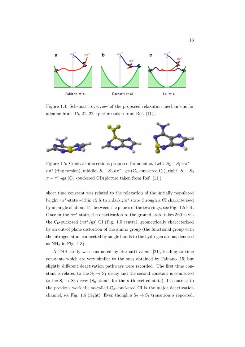
13
Figure 1.4: Schematic overview of the proposed relaxation mechanisms for
adenine from [15, 21, 22] (picture taken from Ref. [11]).
Figure 1.5: Conical intersections proposed for adenine. Left: S2−S1 ππ∗−
nπ∗ (ring torsion), middle: S1−S0 nπ∗−gs (C6 -puckered CI), right: S1−S0
π − π∗ -gs (C2 -puckered CI)(picture taken from Ref. [11]).
short time constant was related to the relaxation of the initially populated
bright ππ∗-state within 15 fs to a dark nπ∗ state through a CI characterized
by an angle of about 15 between the planes of the two rings, see Fig. 1.5 left.
Once in the nπ∗ state, the deactivation to the ground state takes 560 fs via
the C6-puckered (nπ∗/gs) CI (Fig. 1.5 centre), geometrically characterized
by an out-of plane distortion of the amino group (the functional group with
the nitrogen atom connected by single bonds to the hydrogen atoms, denoted
as NH2 in Fig. 1.3).
A TSH study was conducted by Barbatti et al. [21], leading to time
constants which are very similar to the ones obtained by Fabiano [15] but
slightly different deactivation pathways were recorded. The first time con-
stant is related to the S2 → S1 decay and the second constant is connected
to the S1 → S0 decay (Sn stands for the n-th excited state). In contrast to
the previous work the so-called C2−puckered CI is the major deactivation
channel, see Fig. 1.5 (right). Even though a S2 → S1 transition is reported,

14
the system stays in the ππ∗ state, see Fig. 1.4(b). Mean-field analysis by
Lei et al. [22] employing a density functional-based tight binding (DFTB)
approach observed a strong influence of the excitation energy on the relax-
ation path taken and hence on the relaxation times. Using an excitation
energy of 5.0 eV, they observed that the C6−puckered CI is employed for
relaxation. The excited-state lifetime in this case was 1.050 fs. On the other
hand, excitation at 4.8 eV activates the channel through the C2−puckered
CI, with an excited-state lifetime of 1.360 fs.
In all cases the initial ππ∗ state is reported to change to an intermediate
nπ∗ state before reverting to the ππ∗ state and accessing the respective CI.
Accordingly, the authors state that the final transition back to the ground
state happens always from the ππ∗ state, even though previous studies re-
port the C6−puckered CI to be of nπ∗/gs character.
We mention for reason of completeness that Sobolewski, Domcke and cowork-
ers [23, 24], also located another type of CI involving 1σπ∗ states and hy-
drogen abstraction from the NH and NH2 groups, but this proposed decay
pathway will not be discussed further in the present work, where we focus
on the deexcitation processes involving 1ππ∗ and 1nπ∗ states.
To sum up, despite the fact that the time constants predicted by several
groups by using different methods are similar, the predominant relaxation
pathways obtained are different. Depending on the level of theory, either the
state character is preserved [21], leading to the C2-puckered CI, or it changes
to nπ∗ [15], leading to a decay via the C6-puckered CI. It remains unclear
which puckering motion is of major importance until dynamical simulations
at a more reliable level of theory become possible.
1.3 Base multimer excited states
In actual living cells, a nucleobase interacts with other bases within the
same nucleic acid polymer. The structure of nucleic acids allows for interac-
tion within the same strand via stacking and, in the case of double stranded
DNA, also for interactions between two strands via hydrogen bonding (base
coupling), see Fig. 1.6.
What is experimentally observed is that excess electronic energy relaxes

15
(a) (b)
Figure 1.6: Basic assemblies of nucleobases: a)base stacking, b)base pairing
(picture taken from Ref.[2]).
by one or two orders of magnitude more slowly in DNA oligo- and polynu-
cleotides compared to the case of single nucleobases. Moreover, absorption
spectra closely resemble those of the building block monomers, apart from
the decrease of intensity, leading to the well known effect of hypochromism
[25]. In the case of single-stranded adenine homopolymers, both ultrafast
(≈ 1 ps) and more slowly decaying components are observed [7]. Middleton
et al. suggest in Ref. [2] that the fast and slow signal components cor-
respond to excitations in unstacked and stacked base regions, respectively.
The different decay pathways proposed for both stacked and unstacked DNA
single strands are summarized in Fig. 1.7.
The decay in unstacked base strands is hypothesized to occur via the
same pathways illustrated in the previous section for the single monomers:
relaxation along the ππ∗ states, with possible bifurcations to nπ∗ states and
intersystem crossings to triplet states.
The analogous decay behaviour observed for isolated bases and unstacked
single strands is reasonable and intuitive as, in the unstacked geometrical
configuration, single bases are assumed not to be correlated in any way to
each other.
On the other side, strands formed by stacks of two or more bases are ex-
cited to an exciton state. There is strong evidence [26], that regardless of
the length of the sequence, initial excitons trap to a common state that is

16
Figure 1.7: Decay pathways for stacked and unstacked DNA single strands
(picture taken from Ref. [2]).
localized on just two bases. The exciton decays to an exciplex state in less
than 1 ps. The term exciplex/excimer stands for an excited dimer, and it
is generally understood to be formed by an electronically excited monomer
and a second unexcited one. The energy of the two monomers when bound
is lower than the energy of them separated. Here the terms indicate an
excited electronic state with strong charge transfer character. The decay of
excimer/exciplex states by charge recombination takes place in 3 − 200 ps
and may play a dominant role in the photostability of DNA by guaranteeing
that most excited states do not lead to deleterious reactions but instead
relax back to the electronic ground state.
Fig. 1.8 describes the simplest situation of the electronic interactions of
two identical chromophores (A and B) in terms of locally and charge transfer
excited states, depending on the relative position of the excited electron and
the corresponding hole. If they are both located on the same monomer, it is
the case of a locally excited state, while if the electron moves to a different
site, the system gets excited to a charge transfer state.
The wavefunction of the excited state has the general form

17
Figure 1.8: Schematic illustration of the electronic interactions of identical
chromophores A and B in terms of localized and charge transfer excited
states (picture taken from Ref.[27]).
φ(exciplex) = c1Φ(A∗B) + c2Φ(AB∗) + c3Φ(A−B+) + c4Φ(A+B−) (1.1)
where A = B, c1 = c2, and c3 = c4 for excimers. Excimers and exciplexes
are, respectively, excited state complexes formed by two identical or two
different molecules. The first two terms correspond to locally excited states
and their interaction results in exciton states. At intermolecular separations
below 5−6 A, orbital interactions come into play, mediating a mixing of the
locally excited states with the charge transfer states, described by the third
and fourth terms. It is thus important to distinguish whether the exciton
can be described as a linear combination of locally excited states, forming a
Frenkel exciton, or whether CT configurations also play a role. The first case
can be understood in terms of Frenkel exciton theory. In this framework a
model Hamiltonian H is written as the sum of Nmon isolated chromophore

18
Hamiltonians Hm and a coupling term Vml:
H =
Nmon∑m
Hm +∑m
∑l>m
Vml. (1.2)
The singly excited states are described by:
Φa = φexa∏b6=a
φb (1.3)
where the chromophore a is in the excited state, while the others are in the
ground state. The wavefunction of the excitonic state is then written as a
linear combination of the wavefunctions of locally excited states:
Ψk(exciton) =∑a
ckaΦa. (1.4)
When there are strong orbital interactions between the different frag-
ments, Frenkel exciton theory is no longer sufficient and it is necessary to
explicitly include charge transfer configuration in the modeling.
Many models have been developed to investigate the exciton and charge
transfer features in the decay paths of DNA single strands. These models
perform very well in relation to experiments (see Ref. [8] for a relevant
example), but will not be discussed in the following as the current work is
focused on studies of single nucleobases.

Chapter 2
Theoretical background
2.1 Basic notions regarding photophysics in bio-
logical systems
A multitude of processes may occur when sunlight, filtered through the
Earth’s atmosphere, interacts with matter. The spectrum of solar radiation
striking the Earth spans from 100 nm to 106 nm, and can be divided into
the ultraviolet (UV) range (100 nm to 400 nm), visible range (400 nm to
700 nm) and infrared (IR) range (700 to 106 nm).
Molecular photophysical processes relevant for photobiology include absorp-
tion and emission of UV, visible or near-IR light, by molecules. The basic
principles of molecular photophysics can be clarified with the help of the
Jablonski diagram, named after the polish physicist Aleksander Jablonski.
It illustrates the electronic states of a molecule and the transitions between
them, see Fig. 2.1.
19

20
Figure 2.1: Jablonski diagram representing energy levels and related mech-
anisms underlying absorption, fluorescence and phosphorescence spectra.
The singlet states S1 and S2 states, the triplet state T1 and the ground
state S0 involved in the transitions are depicted, including their vibrational
structure (picture taken from Ref. [28]).
The elctronic states are arranged vertically by energy and horizontally
by spin multiplicity. In the left part of the diagram three singlet states with
anti-parallel spin are shown: the singlet ground state (S0) and two higher
singlet excited states (S1 and S2). Singlet states are diamagnetic, as they
do not interact with an external magnetic field. The triplet state (T1) is the
elctronic state with parallel spins. Transistions between electronic states of
the same spin multiplicity are allowed. Transitions between states with dif-
ferent multiplicity are formally forbidden, but may occur due to spin orbit
coupling. Processes of this kind are called intersystem crossings. Superim-
posed on this electronic states are the vibrational states, which are of much
smaller energy.
In Fig. 2.1, solid arrows indicate radiative transitions occurring by ab-
sorption (violet, blue) or emission (green for fluorescence, red for phospho-

21
rescence) of a photon. Dashed arrows represent non-radiative transitions.
Internal conversion is a non-radiative transition, which occurs when a vi-
brational state of higher electronic state is coupled to a vibrational state of
a lower electronic state. In the notation of, for example, S1,0, the first sub-
script refers to the electronic state (first excited) and the second one to the
vibrational sublevel (v = 0). In the diagram the following internal conver-
sions are indicated: S2,4 → S1,0, S2,2 → S1,0, S2,0 → S1,0, S2,0 → S0,0. The
dotted arrow from S1,0 → T1,0 is a nonradiative transition called intersystem
crossing, because it is a transition between states of different multiplicity.
Below the diagram sketches of absorption-, fluorescence- and phosphores-
cence spectra are shown.
When a molecule absorbs a photon of appropriate energy, a valence elec-
tron is promoted from the ground state to some vibrational level in the
excited singlet manifold. The process is extremely rapid (≈ 1 fs = 10−15
s), and this implies that the nuclei of the molecule may be considered as
fixed during the transition, because of their much larger mass, and that the
Born-Oppenheimer approximation (which will be introduced in the follow-
ing) is valid. After light absorption, the excited molecule ends up at the
lowest vibrational level of S1 (S1,0) via vibrational relaxation and internal
conversion, and this radiationless process takes place in about 1 ps (1 ps
= 10−12 s).
In Fig. 2.1, a sketch of an absorption spectrum consisting of two bands is
shown: in the condensed phase, broad absorption bands are observed, rather
than the sharp transitions seen for atoms or molecules in the gas phase.
This is due to the phenomena known as homogeneous and inhomogeneous
broadening. Homogeneous broadening arises from the many vibrational and
rotational states, which are all superimposed on the electronic transitions
preventing the observation of sharp transitions, while inhomogeneous broad-
ening arises from solvent effects.
The strength of the lowest optical transition is very often expressed in terms
of the dimensionless oscillator strenghth f :
f = 1.44 · 10−19
∫ ∞0
ε(σ)dσ (2.1)

22
where ε is the molar extinction coefficient connected with the lowest
electronic transition, σ is the wavenumber and the integral is over the whole
range of wavenumbers of the absorption band. For strongly allowed tran-
sitions f ≈ 1. The oscillator strength has a direct relationship with the
electronic transition dipole moment ~µeg, which couples the wavefunctions of
the ground (Ψg) and excited (Ψe) electronic states. It reads
~µeg =
∫Ψ∗e(r) · ~µ ·Ψg(r)d3r, (2.2)
with ~µ = −er, and the integration takes place over the spatial coordinate r.
This quantity is a measure of the dipole moment associated with the shift of
a charge that occurs when electrons are redistributed in the molecule upon
excitation. The oscillator strength is proportional to the magnitude of the
transition dipole moment, i.e.
f ∝ |~µeg|2. (2.3)
Moving to the central inset of Fig. 2.1, the process of fluorescence is de-
picted. The lowest vibrational level of S1 is the starting point for fluores-
cence emission to the ground state S0, non-radiative decay to S0 (internal
conversion), and transition to the lowest triplet state (intersystem cross-
ing). Fluorescence takes place on the nanosecond timescale (1 ns = 10−9 s),
and, depending on the molecular species, its duration amounts to 1 − 100
nanoseconds. It is clear from the Jablonski diagram that fluorescence always
originates from the same level, irrespective of which electronic energy level is
excited. The emitting state is the zeroth vibrational level of the first excited
electronic state S1,0. It is for this reason that the fluorescence spectrum is
shifted to lower energy than the corresponding absorption spectrum (Stokes
shift). The Stokes shift can be enhanced by solvent interactions. We can
also conclude from the sketched spectra in Fig. 2.1 that the vibrational fine
structure in a fluorescence spectrum reports on vibrations in the ground
state, and vibronic bands in an absorption spectrum provide information on
vibrations in higher electronic excited states.

23
Figure 2.2: Franck Condon principle applied to a two-dimensional poten-
tial energy diagram. The potential wells show favored transitions between
vibrational sublevels ν = 0 and ν = 2 both for absorption (blue arrow)
and emission (green arrow) (picture taken from Wikipedia: Franck Condon
Principle, created by Mark M. Somoza).
Another factor that has to be considered in fluorescence spectroscopy is
the Franck-Condon factor. If we look at the Jablonski scheme in Fig. 2.1,
it can be seen that the fluorescence transition S1,0 → S0,0 is not the most
intense one. The Franck-Condon principle states that the most intense vi-
bronic transition is from the vibrational state in the ground state to that
vibrational state in the excited state vertically above it (Fig. 2.2, blue ar-
row). The schemes (for absorption and emission) in Fig. 2.2 are simplified
two-dimensional potential energy diagrams. Since the excited state is differ-
ent from the ground state, a displaced minimum nuclear normal coordinate
can be expected. It should be noted further that the time to reach the ex-
cited state is so short (femtoseconds) that the nuclei positions are virtually
unchanged during the electronic transition. In the vibronic wavefunctions,

24
the nuclear coordinates can then be uncoupled from the electronic coor-
dinates (Born-Oppenheimer principle). The transition dipole can then be
factorized into an electronic and a nuclear part according to
~µeg =
∫Ψ∗e(r) · ~µ ·Ψg(r)d3relect
∫Ψv(R) ·Ψv(R)d3Rnuc. (2.4)
The second integral is the so-called Franck-Condon vibrational overlap,
which also determines the strength of the electronic transition (or oscillator
strength). In the fluorescent part of the scheme in Fig. 2.1, the second
and third vibrational transitions (S1,0 → S0,1 and S1,0 → S0,2) have larger
Franck-Condon factors than the one between fundamental vibrational wave-
functions S1,0 → S0,0.
In Fig. 2.1, the triplet state is also drawn, from which the process of
phosphorescence arises. Once in a different spin state, electrons cannot relax
into the ground state quickly: they will reside for a very long time there
(from microseconds to seconds) before decaying to the ground state. This is
due to the spin-forbidden transitions involved in the (excited) singlet-triplet
and triplet-singlet (ground state) transitions. As these transitions occur very
slowly in certain materials, absorbed radiation may be re-emitted at a lower
intensity and long-lived phosphorescence from this state can be observed.
Because of its long lifetime, the triplet state of an aromatic molecule is
the starting point for photochemical reactions.
2.2 Born-Oppenheimer approximation and coni-
cal intersections
The theoretical treatment of a molecular system is always based on the
selection of an appropriate computational method, with the final goal of
solving the Schrodinger equation for the whole system. Because of its com-
plexity, the exact solution of the Schrodinger equation is not possible for
most of the molecules of interest. However, the problem can be simplified
by applying procedures leading to satisfying approximate solutions. A basic
approximation on which all quantum chemistry methods are founded is the
Born-Oppenheimer approximation, which will be briefly introduced in the

25
following.
A system of N atoms located at ~R = (R1, R2, ..., Rl, ..., RN ), with n elec-
trons located at ~r = (r1, r2, ..., ri, ...rn) is described by the time-dependent
Schrodinger equation
Hφ(~r, ~R; t) = i~∂
∂tφ(~r, ~R; t) (2.5)
with the total Hamiltonian
H(~r, ~R) = Tn(~R) + Te(~r) + Vnn(~R) + Vne(~r, ~R) + Vee(~r), (2.6)
with
T (~R) = −1
2
N∑I=1
∇2I
MI(2.7)
being the sum of the kinetic energy of the nuclei,
Te(~r) = −1
2
N∑I=1
∇2 (2.8)
being the sum of kinetic energy of the electrons,
Vnn(~R) =N∑I=1
N∑J>1
ZiZj
|~Ri − ~Rj |(2.9)
being the internuclear repulsion,
Vne(~r, ~R) = −N∑I=1
n∑i=1
ZI
|~Ri − ~RI |(2.10)
being the electron-nuclear attraction,
Vee(~r) =
n−1∑i=1
n∑J>1
1
|~ri − ~rj |(2.11)
being the interelectronic repulsion.
MI and ZI denote the mass and atomic number of the I-th nucleus. The
nabla operators ∇I and ∇i act on the coordinates of I-th nucleus and i-th
electron, respectively. Defining the partial electronic Hamiltonian for fixed
nuclei (i.e. the clamped-nuclei part of H) as
Hel = Te(~r) + Vnn(~R) + Vne(~r, ~R) + Vee(~r) (2.12)

26
we rewrite the total Hamiltonian as
H(~r, ~R) = Tn(~R) + Hel(~r, ~R). (2.13)
We assume that the solutions of the time-independent (electronic) Schrodinger
equation,
Hel(~r, ~R)Φk(~r, ~R) = Ek(~R)Φk(~r, ~R), (2.14)
are known for the clamped nuclei, with a discrete spectrum of Hel(~r, ~R) and
orthonormalized eigenfunctions∫ +∞
−∞Φ∗k(~r,
~R)Φl(~r, ~R) ≡ 〈Φk|Φl〉 = σkl. (2.15)
The total wavefunction φ can be expanded in terms of the eigenfunctions
of Hel since these form a complete set, i.e.,
φ(~r, ~R; t) =∑
Φl(~r, ~R)χl(~R, t) (2.16)
Insertion of this so-called Born-Oppenheimer ansatz into the time-dependent
Schrodinger equation (2.13), followed by multiplication from the left by
Φ∗k(~r,~R) and integration over the electronic coordinates, leads to a set of
coupled differential equations
[Tn(~R) + Ek(~R)]χk +∑l
Cklχl = i~∂
∂tχk, (2.17)
where the coupling operator Ckl is defined as
Ckl ≡< Ψk|Tn(~R)|Ψl > −∑l
~2
Ml< Ψk|∇I |Ψl > ∇I . (2.18)
The diagonal term Ckk represents a correction to the adiabatic eigenvalue
Ek of the electronic Schrodinger equation, Eq. (2.14).
The adiabatic approximation is obtained by taking into account only the
diagonal terms, Ckk ≡< Ψk|Tn(~R)|Ψk >, which results in a complete decou-
pling
[Tn(~R) + Ek(~R) + Ckk(~R)]χk = i~∂
∂tχk (2.19)
of the exact set of differential Eqs. (2.17), (2.18). This implies that the nu-
clear motion proceeds without changing the quantum state of the electronic

27
subsystem during time evolution and, correspondingly, the wavefunction
(2.16) is reduced to a single term
φ(~r, ~R; t) ≈ Ψk(~r, ~R)χk(~r, ~R), (2.20)
being the direct product of an electronic and a nuclear wavefunction. The
last simplification consists in also neglecting the diagonal coupling terms
[Tn(~R) + Ek(~R)]χk = i~∂
∂tχk (2.21)
which defines the Born-Oppenheimer approximation. The Born-Oppenheimer
approximation can be applied to a considerable number of physical situa-
tions. However, many theoretical and experimental studies have revealed
cases where the Born-Oppenheimer approximation fails, meaning that the
total wavefunction is not well approximated by a simple product of an elec-
tronic eigenfunction with a vibrational wavefunction (the eigenfunction of
the nuclear part of the Schrodinger equation). A particularly relevant fail-
ure is encountered in the vicinity of PES crossings (for degenerate or nearly
degenerate electronic states). There, molecular motion is determined not
only by the PES of the given state but depends also on the topology of the
(almost) degenerate PES.
A potential energy surface is the result of solving equation (2.14) for
many nuclear configurations, leading to the electronic potential energy as a
function of the nuclear coordinates.
In a diatomic molecule there is only one nuclear coordinate, the interatomic
distance RAB. In this case, the potential energy ‘surface’ is more accurately
termed a potential energy curve. It describes the potential energy of the
system, U(RAB), as the two atoms are brought closer to, or moved away
from each another.
The concept can be expanded to a tri-atomic molecule such as water
where we have two O-H bonds and H-O-H bond angle as variables on which
the potential energy of a water molecule will depend. The two O-H bonds
can be safely assumed to be equal. Thus, a PES can be drawn mapping
the potential energy E of a water molecule as a function of two geometrical
parameters, q1 = O-H bond length and q2 = H-O-H bond angle. The lowest

28
point on such a PES will define the equilibrium structure of a water molecule.
In Fig. 2.3 a water molecule PES is depicted, including the energy minimum
corresponding to the optimized molecular structure for water- O-H bond
length of 0.0958 nm and H-O-H bond angle of 104.5.
Figure 2.3: PES for a water molecule. The figure shows the energy minimum
corresponding to the optimized molecular structure for water: O-H bond
length of 0.0958 nm and H-O-H bond angle of 104.5 (picture taken from
Wikipedia: Energy profile (chemistry), created by AimNature)).
When computing multiple potential energy surfaces for a system, for
instance, the ground state and electronic excited states, the possibility of
the surfaces having the same value of potential energy, U(R), occurs. This
might be the case, for example, in which a minimum on the upper surface
comes into the region of a maximum on the lower surface. What happens at
this point is not of straightforward interpretation, a simplified mathematical
treatment is given in the following.
The non-crossing rule was quantitatively formulated in 1929 by von Neu-
mann and Wigner [29], proving the theorem put forward earlier by Hund
[30], and stating that potential energy curves corresponding to electronic
states with the same symmetry properties cannot cross.

29
Figure 2.4: An avoided energy-level crossing in a two-level system subjected
to an external magnetic field (picture taken from Wikipedia: Adiabatic
theorem).
Von Neumann and Wigner gave the mathematical proof for Hund’s ar-
gument, given here in a contracted form.
Whenever two energy levels E1 and E2 come close to each other, the cou-
pling V between the corresponding states is not negligible. The 2×2 matrix
Hamiltonian describing the system is given by
H =
∣∣∣∣∣E1 V
V E2
∣∣∣∣∣ . (2.22)
If the two energies depend on some parameter, e.g. in an approximately
linear way, there may be a point where they are degenerate. The eigenvalue
equation
∣∣∣∣∣E1 − E V
V E2 − E
∣∣∣∣∣∣∣∣∣∣c1
c2
∣∣∣∣∣ = 0 (2.23)
leads to eigenvalues of the Hamiltonian which will not become degenerate,
but will have a hyperbolic shape where the minimal energetic distance is
2V . This is called an avoided crossing. In the (avoided) crossing region, the

30
two states (e.g. one photonic and the other electronic excitation) become
strongly mixed.
Thus far, we have been concerned with potential energy surfaces derived
within the Born-Oppenheimer approximation, also known as the adiabatic
approximation. Hence, such surfaces are referred to as adiabatic potential
energy surfaces. A surface where actual intersections are substituted for the
avoided crossings is termed a diabatic surface. If the nuclei are assumed to
move slowly, then they are likely to follow a single, adiabatic energy surface,
even in the region of an avoided crossing. If the nuclei have sufficient velocity,
then the Born-Oppenheimer approximation breaks down and the nuclei may
effectively “ignore” the gap in the avoided crossing and simply cross over
to the other adiabatic surface, adopting that configuration. This is termed
non-adiabatic or “diabatic”.
Conical intersections are interesting as they exist between adiabatic surfaces,
where we would usually expect an avoided crossing. The distortion observed
at a conical intersection is a consequence of the breakdown of the Born-
Oppenheimer approximation. At a conical intersection, one can distinguish
two directions, X1 and X2, such that if the energy in the subspace (the
branching space) of these two geometric variables changes (combinations of
the bond lengths, angles, etc.), the potential energy would have the form of
a double cone in the region of the degeneracy. The remaining n–2 directions
define the crossing surface (the intersection space) in which the energies of
ground and excited states are equal. A movement in the plane (X1,X2) from
a point on the intersection will result in the degeneracy being lifted. The
two vectors X1 and X2, defined as
X1 =∂(E1 − E2)
∂q(2.24)
X2 = 〈ct1|∂H
∂q|c2〉, (2.25)
correspond to the gradient difference vector and non-adiabatic coupling vec-
tor, respectively, see Fig. 2.5.

31
Figure 2.5: A conical intersection as described by a double cone geometry
using two variables, X1 and X2 (picture taken from: iupac.org, Conical
intersections).
The main feature of a conical intersection is its non-adiabatic nature:
it is the breakdown of the Born-Oppenheimer approximation that allows
non-adiabatic electronic transitions to take place. Clearly, conical inter-
sections facilitate easier transitions compared to avoided crossing, allowing
radiationless decay.
2.3 Theory of 2D electronic spectroscopy
Linear spectroscopy measures the first-order polarization induced in a
sample by a single interaction with the incident electric field. The most
basic method of linear absorption spectroscopy involves a weak light-matter
interaction with one primary incident radiation field, and gives a picture
of the first excited state manifold of the sample, projected onto a single
frequency axis. Transition dipole strengths and excitation energies can be
probed, but there is no explicit information about coupling between different
excitons or excited state absorption.

32
In complex systems, where many interacting degrees of freedom are present,
the interpretation of linear spectra has to deal with a number of ambiguities.
Two representative examples are given in the following.
When an absorption spectrum shows two peaks (see Fig. 2.6), a reasonable
question is if these arise from different, non-interacting molecules, or are
coupled quantum states of the same molecule. No answer can be obtained
from linear absorption spectroscopy, since it cannot resolve couplings or
spectral correlations directly, see Fig. 2.7.
Figure 2.6: Absorption spectrum with two peaks (picture taken from:
Tomakoff Group, Nonlinear and Two dimensional Spectroscopy Notes).
Figure 2.7: Left: excitation of different, noninteracting molecules. Right:
coupled quantum states of the same molecule (picture taken from: Tomakoff
Group, Nonlinear and Two dimensional Spectroscopy Notes).
Another ambiguous situation one could have to face is the interpretation
of broad lineshapes. Distinguishing whether a broadened spectrum comes

33
from a homogeneous lineshape broadened by fast irreversible relaxation or
an inhomogeneous lineshape arising from a static distribution of different
frequencies (see Fig. 2.8) is not an easy task, because linear spectra cannot
uniquely interpret line-broadening mechanism, or decompose heterogeneous
behavior in the sample.
Figure 2.8: Homogeneous (left) and inhomogeneous broadening (right) (pic-
ture taken from: Tomakoff Group, Nonlinear and Two dimensional Spec-
troscopy Notes).
Spectroscopy is the primary tool for describing the molecular structure,
interactions and relaxation, the kinetics and the dynamics of such systems.
Nonlinear spectroscopy can be used to correlate different spectral features.
This technique presents spectroscopic data as a map of spectral interactions
between two frequencies, ω1 and ω2. They can be thought of as excitation
and detection frequencies, respectively.
Two dimensional electronic spectroscopy (2DES) probes the third order po-
larization generated by the interaction of three carefully timed laser pulses
with the sample of interest. First, a broadband pump pulse interacts with
the sample, exciting a quantum mechanical coherence between the ground
and first excited states. After a time t1, frequently called the coherence
time, a second pump pulse interacts with the sample, creating a population
in the ground or excited electronic state. The time t2 before the third pulse
arrives is often referred to as the population time, and it is here that many
of the interesting dynamics such as energy and charge transfer occur.
The probe pulse creates a second coherence in the sample, which leads
to signal emission at a time t3 after the probe pulse, based on one of two
major processes. The first of these, in which the phase progression reverses
in comparison to the first coherence, is called the “rephasing” signal or
“photon echo”. The other follows a free-induction decay along the original

34
phase progression and is called a “non-rephasing” signal or sometimes a
“virtual echo”. To reconstruct a true absorptive 2D spectrum, both of these
signals must be obtained and properly combined [31, 32, 33]. The real part of
the complex 2DES spectrum will give the absorptive part and the imaginary
part produces a dispersive component.
2.3.1 Polarization and density matrix
The theory applied to 2D spectroscopy is generally a mixed quantum-
classical framework, in which the incident fields are treated classically, but
the material system is described quantum mechanically. The treatment of
the bath and the system-bath coupling usually involves averaging over bath
degrees of freedom and the system is described by a density matrix ρ. The
diagonal elements ρii represent populations, while the off-diagonal elements
ρij give the coherences.
In situations of weak excitation, the time dependence of the density matrix
may be expanded perturbatively in powers of the incident electric field:
ρ(t) ≡ ρ(0)(t) + ρ(1)(t) + ρ(2)(t) + ... (2.26)
where ρ(n)(t) represents the n−th order contribution of the electric field.
The n−th order density matrix cannot be measured directly. However, it
can be probed by measuring the n−th order macroscopic polarization, which
is related to the expectation value of the dipole operator µ:
P (n)(r, t) = Tr[µρ(n)(r, t)] (2.27)
The first order polarization is responsible for linear optical effects. The
second order polarization P (2) is involved with nonlinear properties in bire-
fringent media, such as sum and difference frequency generation. It can
be shown that the signal contribution from P (2) vanishes in isotropic me-
dia. Therefore, the next term of interest after the linear optics is P (3), the
third order polarization. It is this order that is probed in 2D electronic
spectroscopy and other four-wave mixing spectroscopies, such as transient
absorption spectroscopy. In the following P (3)(r, t) will be the quantity of
interest.

35
In the time domain, the third order polarization is a time convolution of
the incident electric fields with the third order material response function
R(3)(t3, t2, t1) [34]:
P (3)(r, t) = N
∫ ∞0
dt3
∫ ∞0
dt2
∫ ∞0
dt1R(3)(t3, t2, t1)E3(r, t− t3) (2.28)
E2(r, t− t3 − t2)E1(r, t− t3 − t2 − t1)
where R(3) is the third order response function given by
R(3)(t3, t2, t1) =
(i
)3
〈Vν4|G(t3)Vν3G(t2)Vν2G(t1)Vν1|ρ0〉. (2.29)
The response function describes the full time-dependent, microscopic state
of the system for any set of three input pulses arriving at times ti. The
system is initially in the equilibrium state described by the density matrix
ρ0. The dipole operator Vνi modifies the density matrix following interaction
with the i-th pulse, and the field-free molecular time evolution for an interval
ti is given by the Green’s function G(ti). The final interaction Vν4 is the
signal mode giving the final response.
We assume delta function pulses, such that the time intervals are well defined
and well-ordered, and the pulses are much shorter than the investigated
molecular dynamics. Then, the incoming electric field can be expanded in
modes according to
E(r, t) =∑j
εj(t) exp(ikj · r− iωjt) + exp(−ikj · r + iωjt), (2.30)
where ε(t) is the temporal pulse envelope and the summation index j is over
the pulse number (input pulses 1-3 and signal s). For the visible and near-IR
wavelengths used in 2DES experiments, the pulse wavelengths (400-800 nm)
are much lower than the sample size and the approximation kjr 1 holds.
Therefore, in 2DES experiments, the signals are highly directional, and the
signals related to specific energy pathways are chosen through a phase-
matching condition. The response function can then be expanded as
R(3)(t3, t2, t1) =
(i
)3∑l
R3l (t3, t2, t1) exp(ikl · r− iωlt) (2.31)

36
The Rl are the response function components associated with each pathway
in the signal. Because there are three input pulses, and each pulse can
interact with either the ket or the bra (positive or negative frequency), there
are 23 = 8 different signals over which the index l iterates. The phase and
frequency matching conditions for these are
kl = ±k1 ± k2 ± k3, (2.32)
ωl = ±ω1 ± ω2 ± ω3 (2.33)
The cases in which all the frequency components have the same sign are
highly oscillatory and do not contribute largely to the signal and can be ne-
glected by employing the rotating wave approximation. The dominant sig-
nals of interest in 2DES are usually referred to as the photon echo, or rephas-
ing, signal (ks = −k1 +k2 +k3) and the non-rephasing (ks = +k1−k2−k3).
The terminology comes from the fact that the phase evolves at conjugate
frequencies during the two coherence periods in the rephasing signal but not
in the non-rephasing. Thus the former is able to reform into an “echo”, while
phase evolution in the latter can only continue in the same direction. Con-
tributions to the signal in directions that do not match the phase-matching
condition will vanish due to a randomness in the phase [35].
The mathematical notation necessary to describe the various signal path-
ways associated with the field-matter interactions and density matrix field-
free evolution periods can get very complicated. In double sided Feynman
diagrams we find a simple tool for graphically representing the various path-
ways of the time evolution of the density matrix [35, 36].
The Feynman diagrams for the rephasing and non-rephasing pathways are
shown in Fig. 2.9 along with the corresponding energy level diagrams. These
include contributions from ground state bleach (GSB), excited state emis-
sion (ESE) and excited state absorption (ESA), as well as diagrams related
to features with common ground states (CGS) or energy transfer (ET).
For a detailed explanation of the formalism underlying double sided Feyn-
man diagrams, see Ref. [34].
In the general case of pathways involved in 2DES, the first pulse will
interact with either the ket or the bra. A single pulse interaction places

37
Figure 2.9: Double-sided Feynman diagrams for the rephasing and non-
rephasing pathways. The energy levels below show the pulse interactions
corresponding to each Feynman diagram. Dotted (solid) lines denote in-
teractions with the ket (bra) (picture taken from Ref. [37]).

38
the sample in a coherent superposition state, represented by an off-diagonal
element in the density matrix ρij , which oscillates at the frequency of ab-
sorption during the coherence time t1 as illustrated in Fig. 2.10.
Figure 2.10: A diagram of the density matrix elements involved during co-
herence and population times for a rephasing signal (picture taken from Ref.
[37]).
This coherence decays rapidly due to dephasing processes. After the
free evolution with the Green function G(t1), the second pulse interaction
creates a population in either the ground or excited state, corresponding to
a diagonal element in the density matrix ρii. The time between the second
and third pulses (t2) is often called the “population time”. It is during
this long-lived period that most of the interesting system dynamics occurs,
including for instance energy transfer and charge separation. The third pulse
again creates a coherence in the sample. Depending on the frequency of the
interaction and available manifold of states, this coherence can be between
the ground and first excited state or between the first and second excited
state, in the case of excited state absorption. The signal field radiates at
a time t3 after the third pulse in a phase matched direction determined by
the pathway involved.

39
2.3.2 2D spectra
The 2D spectrum contains information about both coherence periods,
t1 and t3. Generally, t1 is scanned in small steps and Fourier transformed
to a frequency axis ω1. This axis contains information about the transition
to the first excited state and can be considered as a label of the initial
excitation frequency. In most cases, the delay t3 is measured directly in
the frequency domain ω3 to facilitate easier data collection. ω3 contains
frequency information about the second coherence, which is related to the
frequency of the third pulse, which probes the state of the sample following
the dynamics during the t2 period. Therefore, the 2D spectrum acts as a
correlation map, wherein the ω1 axis can be thought of as the “excitation
axis” and ω3 is considered the “detection axis”. The t2 delay is fixed for
a given spectrum. So, each 2D spectrum is like a snapshot of the sample
state at a specific value of t2. To analyze the kinetics, several spectra must
be taken for different values of t2. A complete scan over t2 will give a 3D
spectrum S(ω1, t2, ω3).
To illustrate the types of information available in 2DES data, a cartoon
of a simple 2D spectrum is shown in Figure 2.11 along with energy level
diagrams indicating the transitions involved in the case of a pair of coupled
three-level systems. For cases in which the sample absorbs and emits at the
same frequency, a peak shows up along the diagonal, while energy transfer
and electronic coupling show up as a cross-peak below the diagonal. Cross-
peaks above the diagonal also occur but have generally lower amplitude due
to the low probability of uphill energy transfer in most coupling schemes.
Excited state absorption is shown as a negative amplitude peak shifted from
the diagonal by the anharmonicity. The spectrum also gives a direct measure
of the homogeneous and inhomogeneous linewidths as the antidiagonal and
diagonal peak widths, which can be used to obtain the frequency-frequency
correlation function for a given value of t2 [38].
To analyze the sample kinetics or any other population dynamics, a series
of 2D spectra are acquired, each for a different value of t2: in this way a
complex 3D array of data S(ω1, t2, ω3) is obtained. Each 2D spectrum is a
frequency-frequency correlation map: given that a chromophore is excited

40
Figure 2.11: Representation of a 2DES spectrum and associated energy level
diagrams for a pair of coupled three-level systems (picture taken from Ref.
[37]).
at a frequency ω1, the 2D spectrum shows directly the distribution of fre-
quencies ω3 at which the sample emits or absorbs after a time t2.
The information content of a transient absorption (TA) experiment is the
same as that of a 2D spectrum integrated over the excitation (ω1) axis.
Analysis of transient absorption (or pump probe) spectra is one of the main
points we are going to discuss, among the results presented in this work, see
Chapter 5. 2DES is an ideal method for the study of condensed phase sys-
tems, including biological complexes in solution, in which the local solvent or
protein environment introduces a large degree of inhomogeneous broadening.
The technique can reveal homogeneous lineshapes beneath inhomogeneously
broadened spectra to provide insight into the physical nature of the broad-
ening. It can also capture couplings, energy and charge transfer, and other
rapid spectral dynamics with high time resolution [39].

Chapter 3
Computational methods
3.1 Quantum chemistry calculations
The past few decades have witnessed the development of a hierarchy of
quantum chemical methods that can be used to investigate the structures
and properties of molecules and solids [40, 41].
Several methods exist with completely different approaches to the solution
of the main problem in quantum chemistry, which is the integration of the
Schrodinger equation for the considered system. Since an exact solution
of the problem is impossible for almost any kind of system, approxima-
tion methods are required, which allow to determine electronic structure,
to optimize the geometry of molecules and to calculate excitation ener-
gies/frequencies and charge distributions.
Properties and reactions in the electronic ground state can be studied rou-
tinely by computation: high-level ab initio methods, such as the coupled
cluster theory and the Møller–Plesset perturbation theory [42, 43], give ac-
curate predictions for ground-state properties, while fast semiempirical ap-
proaches are used for treating large systems [44, 45].
Because of its favorable cost-performance ratio, density functional theory
(DFT) is used widely and successfully in studies of chemical reactions [46],
and this is the case of the current investigation on nucleobases as well.
41

42
3.1.1 Time-Dependent Density Functional Theory (TDDFT)
Generally, two categories of quantum chemical approaches exist for the
calculation of excited states. The first kind is the wave-function-based ap-
proach, such as the Configuration Interaction (CI), the Multi-Configurational
Self-Consistent Field (MCSCF) and the Complete Active Space Perturba-
tion Theory of second order (CASPT2) method [47].
When the number of electrons increases, the wavefunctions become much
more complicated and will cost more computing time. Electron-density-
based methods become then more convenient, such as time-dependent den-
sity functional theory (TDDFT), where the calculation makes use of func-
tionals of the electronic density, and the approximation is due to the proper
estimation of the functionals.
TDDFT methods can be very accurate for little computational cost. In re-
cent years, they have been widely used to deal with photochemical properties
from small to medium molecules and even large biological systems. In this
subsection, we will focus on this popular class of computational methods for
excited states.
In density functional theory, the electron density of a molecule is used to
determine the energy and derivative properties of molecules. The electron
density only depends on three spatial coordinates. It is a function with three
variables: x-position, y-position, and z-position of the electrons, ρ(x, y, z).
The energy of the molecule is then a functional of the electron density:
E = F [ρ(x, y, z)] (3.1)
So there is a one-to-one mapping between the electron density of a sys-
tem and the energy. We can get considerable information about a molecule
if we can determine its electron density, which is the fundamental quantity
on which density functional theory is based. Compared to ab initio meth-
ods, the electron density function is only dependent on three coordinates,
independent of the system size. This approach is much faster than ab initio
methods.
However, despite its widespread popularity and success, TDDFT still has

43
limitations in its present form. For instance, the approach fails for strongly
correlated systems and underestimates the barriers of chemical reactions and
charge transfer excitation energies [48].
The density functional theory is based on the Thomas–Fermi model [49]
(developed by Thomas and Fermi in 1927) and the Hohenberg-Kohn theorem
[50, 51], set up in 1964 by Hohenberg and Kohn. The first Hohenberg-Kohn
theorem states that the ground state electron density uniquely determines
the potential and thus all properties of the system, including the many-
body wave function. The second Hohenberg-Kohn theorem guarantees the
existence of a variational principle for electron densities. Kohn and Sham
introduced the Kohn-Sham orbitals and developed the Kohn-Sham theory,
bringing the density functional theory into a more practical version. In the
Kohn-Sham theorem, the total energy E[ρ] is expressed as
E[ρ] = Ts[ρ] + J [ρ] + Ene[ρ] + EXC [ρ], (3.2)
where Ts[ρ] is the kinetic energy of a non-interacting system, J [ρ] is the clas-
sical electron-electron repulsive (Coulombic) energy, Ene[ρ] is the nuclear-
electron attraction energy. The exchange-correlation term EXC [ρ] contains
the exchange and correlation effects. In density functional theory, all the
approximations lie in the exchange-correlation term. The Kohn-Sham equa-
tion is given by
HKSΦKSi = εiΦ
KSi (3.3)
where the Hamiltonian HKS can be expressed as:
HKS(r) = −1
2∇2 + VKS(r) (3.4)
where
VKS(r) = Vne(r) +
∫ρ(r′)
r− r′dr′ + VXC(r) (3.5)
and VXC [r] is the exchange-correlation term. Equation (3.3) is limited to
time-independent systems. The Runge-Gross Theorem [52] is an analogous
time-dependent version of the first Hohenberg-Kohn theorem. It states that
two external potentials v(r1, t) and v(r2, t), which differ by more than a

44
time-dependent constant C(t), result in two different electron densities, that
is:
v(r1, t) 6= v(r2, t) + C(t)→ ρ(r1, t) 6= ρ(r2, t). (3.6)
So there still exists a unique relationship between time-dependent potentials
V (r, t) and time-dependent densities ρ(r, t). Therefore the property of a
system can be written as a functional of the time-dependent density. The
Runge-Gross theorem is the rigorous mathematical basis of TDDFT. This
is the first step for the extension to the time domain. The next step is the
existence of a time-dependent variational principle that is analogous to the
second Hohenberg-Kohn theorem [53, 54].
If the wave function Ψ(r, t) is the solution of the time-dependent Schrodinger
equation,
i∂
∂tΨ(r, t) = H(r, t)Ψ(r, t), (3.7)
it is the stationary point of the action integral
A =
∫ t1
t0
dt〈Ψ(t)|i ∂∂t− H(t)|Ψ(t)〉. (3.8)
According to the Runge-Gross theorem, the action integral can be written
as a functional of the time-dependent density:
A[ρ] =
∫ t1
t0
dt〈Ψ[ρ](r, t)|i ∂∂t− H(r, t)|Ψ[ρ](r, t)〉. (3.9)
To derive the time-dependent Kohn-Sham equation, a time-dependent non-
interacting reference system exists according to van Leeuwen [54]. The time-
dependent Kohn-Sham equation is written as
i∂Ψi(r, t)
∂t=
(−1
2∇2i + v(r, t) +
∫d3r′
ρ(r′, t)
|r− r′|+δAXC [ρ]
δρ(r, t)
)Ψi(r, t)
(3.10)
In this case, the AXC part contains all the exchange and correlation effects.
There are different approximations for this functional. The DFT theory is
extended to the time-dependent domain and developed to time-dependent

45
density functional theory (TDDFT). Using TDDFT in linear response (de-
riving the linear response of the time-dependent Kohn-Sham equation) al-
lows us to obtain useful information, such as excitation energies and oscil-
lator strengths of excited states.
TDDFT has become one of the most popular quantum chemical tools to
calculate excited-state properties of medium-sized or even large biological
molecules from first principles. While accurate high-level calculations such
as CASPT2 and CASSCF employing large active spaces are tedious and time
consuming, the TDDFT calculation can reach the accuracy of sophisticated
quantum chemical methods with moderate computational cost. However, as
we already mentioned, there are shortcomings in TDDFT. For instance, the
choice of the right exchange-correlation functional for the given excited state
property is crucial. As an example, the hybrid functional B3LYP is unsuc-
cessful in some applications: for instance, the lack of long range correlation
causes the failure of the approach for treating charge transfer (CT) problems.
In the present studies the TDDFT implementation in the GAUSSIAN
quantum chemistry program package has been applied. The functional
M062X has been used for the TDDFT calculations.
The M06-2X and CAMB3LYP functionals have been chosen for the purposes
of the present study because they perform reasonably well in linear response
TDDFT calculations for molecular clusters. In particular, they avoid un-
derestimation of the energies of the states involved in charge-transfer tran-
sitions, and do not predict spurious charge- transfer transitions to occur at
low energies [55].
3.1.2 Basis sets
Given the calculation method, a basis set has to be chosen to optimally
approximate the wavefunction. It is composed of a set of functions, which
are linearly combined to approximate molecular orbitals.
A good description is given by Slater-type orbitals (STOs):
R(r) = Nrn−1e−ζr (3.11)

46
where n is the quantum number, N is the normalizing constant, r is the dis-
tance of the electron from the atomic nucleus, and ζ is the constant related
to the effective charge of the nucleus.
As they decay exponentially with the distance from the nuclei, STOs accu-
rately describe the long-range overlap between atoms, and reach a maximum
at zero, well describing the charge and spin at the nucleus. Due to compu-
tational difficulties in realizing them, approximations as linear combination
of Gaussian orbitals (GTOs) are more convenient and are mostly chosen for
the actual calculations. Hence, in fact, we have
R(r) = Brle−αr2
(3.12)
where l is the angular momentum, and α is the orbital exponent. Since it is
easier to calculate overlap and other integrals with Gaussian basis functions,
this leads to a huge computational advantage.
There are hundreds of basis sets composed of GTOs, the smallest are called
minimal basis sets, and they are typically composed of the minimum number
of basis functions required to represent all the electrons on each atom. The
most common ones are called STO-nG, where n is the number of Gaussian
primitive functions comprising a single basis function. Correlation consis-
tent basis sets (CCBSs) are also used, since they are designed to converge
to the complete basis set (CBS) limit. Basis sets of this kind are cc-pVNZ,
where N=D,T,Q,5,6,... (D=double, T=triples, etc.). The “cc-p” stands
for “correlation-consistent polarized” and the “V” indicates that they are
valence-only basis sets. The most common extension to basis sets is the
addition of polarization functions, denoted by a ∗. An improvement of the
accuracy also could be reached by making use of “augmented” basis sets,
i.e., by using very shallow Gaussian basis functions, which more accurately
represent the tail portion of the atomic orbitals, which are distant from the
atomic nuclei. This is important for large “soft” molecular systems.
As already mentioned, the functionals M062X and CAMB3LYP have
been used for the TDDFT calculations of the current studies, with the aug-
cc-pVDZ and aug-cc-pVTZ basis sets.

47
3.2 Semiclassical nuclear ensemble method
In the current work, linear absorption spectra have been simulated for
the main tautomers of nucleobases in their hydrosolvated molecular geom-
etry. The UV-VIS absorption spectra in aqueous solution were modelled
using the semiclassical nuclear ensemble method of Crespo-Otero and Bar-
batti [56]. This method allows the performance sophisticated simulations
on molecular systems with a high degree of chemical complexity, taking into
account several effects, such as vibrational broadening and solvent effects.
It is based on the approximation that the forms of spectral bands are pre-
dominantly controlled by the nuclear geometry distribution of the electronic
ground state [56]. This approach requires as input a set of Npts ground-
state geometries of the molecule of interest Ri, which are usually sam-
pled either from a statistical distribution or from thermostatted molecular
dynamics trajectories. The vertical excitation energies ∆E0n(Ri) for the
excitation to the n-th excited state and the associated oscillator strengths
f0n(Ri) are computed at each of these geometries. Then, the molecular
absorption cross-section σ is calculated as
σ(E) =πe2~
2me cε0nrE
Nfs∑n=1
1
Npts
Npts∑i=1
∆E0n(Ri)f0n(Ri)g(E −∆E0n(Ri), δ).
(3.13)
Here, g(E−∆E0n(Ri), δ) is a normalized line-shape function whose purpose
is to account for other sources of broadening, such as collisions and finite
excited-state lifetime. In practice, the simulated spectra are found to be rel-
atively insensitive to the choice of the line-shape function [57]. nr denotes
the index of refraction of the medium, and me is the electron rest mass. Nfs
is the number of vertical excitation energies calculated for each configura-
tion. In turn, the molecular absorption cross-section σ (expressed in cm2)
is related to the molar extinction coefficient ε (in M−1 cm−1) through
ε =NA × 10−3
ln(10)σ. (3.14)
The nuclear ensemble method simulates only the envelopes of spectral bands,
and cannot predict fine spectral features such as vibrational progressions.
For the purposes of the present work, however, this does not represent a

48
serious drawback, as such features are also unresolved in experimentally de-
termined spectra of nucleobases in solution.
For each molecule under study, Npts = 500 geometries were sampled from
the Wigner quantum harmonic oscillator distribution for the vibrational
ground state, which was generated using the program initcond.pl from the
simulation package Newton-X [59, 60]. Nfs = 15 vertical excitation energies
were calculated for each such geometry. A Gaussian line-shape function
g(E −∆E0n(Ri), δ) =
√2
δ2πexp
(−2(E −∆E0n(Ri))
2
δ2
)(3.15)
was used, with the broadening parameter set to δ = 0.2 eV. The index of
refraction of the aqueous solution was taken to be independent of the wave-
length, with a value of nr = 1.36. In the present studies, the implementation
in the GAUSSIAN quantum chemistry program packages has been applied
[61]. The functionals M062X and CAMB3LYP with the aug-cc-pVDZ basis
set have been used for the TDDFT calculations.
The results obtained for linear absorption spectra of nucleobases by applying
the semiclassical nuclear ensemble method are described in Chapter 4.
3.3 TNL and HEOM methods for the solution of
Non-markovian Master Equation
Molecules in solution are under the influence of the environment, which
leads, among other effects, to strong damping of vibrational motion. There-
fore, it is necessary to employ simulation methods that include the effect
of environmental damping. While damping can be included in the wave
function formalism of quantum mechanics at a phenomenological level, only
the density matrix formalism allows a proper treatment of decoherence and
dissipation.
The employed methods for the treatment of adenine in aqueous solution as
an open quantum system will be presented in the following. This sets the
framework for the calculations of 2D spectra discussed in Chapter 5.

49
3.3.1 Open quantum systems
In the experimental reality, any system is in contact with a solution
(hereafter called environment or bath) and therefore must be treated as an
open quantum system. The whole system (system+environment) can be
well described by the following model Hamiltonian [58, 64]
Htotal = Hs +Hb +Hsb, (3.16)
where Hs is the system Hamiltonian, Hsb is the system-environment cou-
pling, and Hb is the Hamiltonian model for the bath. Additionally, we can
consider a factorized initial state W (t = t0) = ρ(t0)⊗ R0 at an initial time
t0 when the interaction is turned on. There, ρ(t0) and R0 are the initial
state of the system and the environment, respectively. The latter can be as-
sumed to be formed by a collection of harmonic oscillators, which generate
Gaussian fluctuations for the system of interest [58, 64].
In the simplest case, one can assume the weak coupling regime and invoke
the Markov approximation, neglecting any memory effects on the dynamics
of the reduced density matrix ρ(t). The latter is obtained after the harmonic
bath has been traced out. In the regime of weak coupling, the Born approx-
imation is performed as well, leading to the Born-Markov master equation
for the reduced density operator. The bath is only of indirect interest, and
its properties need only to be specified in general terms, e.g., by the tem-
perature and its spectral density function. The simplest case is the one of
frequency independent damping, which is realized by an Ohmic spectral den-
sity J(ω) = mγωe−ω/ωc . Therein, γ and ωc are the damping constant and
a cut-off frequency, which is taken to be the largest frequency in the model.
The reduced density matrix ρ(t) then evolves according to the equation of
motion
ρ(t) = D[ρ(t)], (3.17)
where D is the Liouvillian superoperator, which is composed of a coherent
part L0 describing the dynamics of the uncoupled system, and a dissipative
part L encompassing the dissipative effects and yielding to the transition
rates for the relaxation processes, i.e.
D = L0 + L . (3.18)

50
The most convenient way to integrate Eq. (3.17) is to solve the eigenvalue
problem for D [65]. The latter is not a hermitian operator, i.e., in general
we cannot find a set of eigenoperators where D is diagonal. However, it is
possible to find its right and left eigenoperators,
Dvk = λkvk, (3.19)
vkD = λkvk, (3.20)
where λk are complex numbers. Solving the above eigenvalues problem,
the reduced density operators can be written as:
ρ(t) =∑k
ckeλktρk + ρ∞ (3.21)
where ck = Trρ(0)v†k
, and ρ∞ corresponds to the right eigenvector with
zero eigenvalue. For a more detailed treatment of theory and calculations,
see Ref. [65].
Many attempts have been made to go beyond the Markov approxima-
tion. One of the available approaches is a time nonlocal method based on a
numerical decomposition of the spectral density [66]. We will describe this
Time Nonlocal (TNL) method in the following.
3.3.2 Time Nonlocal method
The total Hamiltonian of the system-plus-bath complex can be written
as the sum of four terms,
H = Hs +Hb +Hsb +Hren, (3.22)
where Hs is the system Hamiltonian, Hsb is the system-environment
coupling, Hb is the Hamiltonian model for the bath and Hren is the renor-
malization term. In
Hs =p2
2M+ V (q) +W (q, t), (3.23)
the potential is split into a time-independent part V (q) and an explicitly
time-dependent part W (q, t) which, for example, may represent a laser field.
The bath Hamiltonian is taken as the sum of harmonic oscillators with mass
mi and frequency ωi:
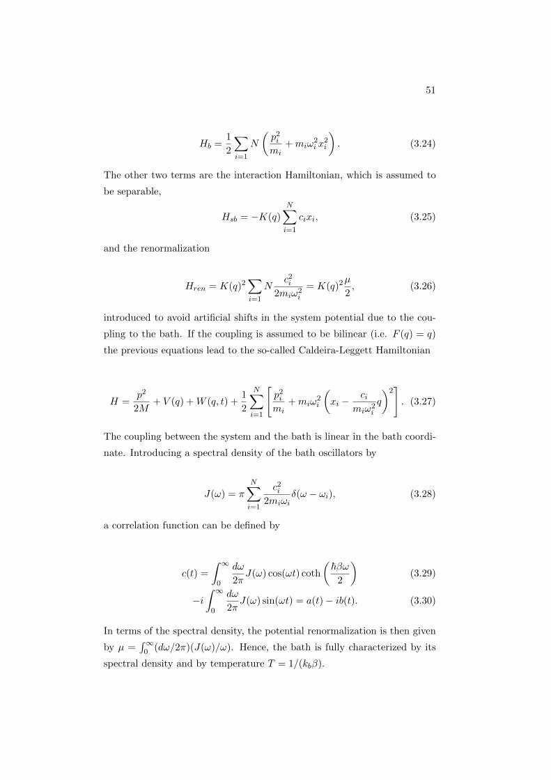
51
Hb =1
2
∑i=1
N
(p2i
mi+miω
2i x
2i
). (3.24)
The other two terms are the interaction Hamiltonian, which is assumed to
be separable,
Hsb = −K(q)
N∑i=1
cixi, (3.25)
and the renormalization
Hren = K(q)2∑i=1
Nc2i
2miω2i
= K(q)2µ
2, (3.26)
introduced to avoid artificial shifts in the system potential due to the cou-
pling to the bath. If the coupling is assumed to be bilinear (i.e. F (q) = q)
the previous equations lead to the so-called Caldeira-Leggett Hamiltonian
H =p2
2M+ V (q) +W (q, t) +
1
2
N∑i=1
[p2i
mi+miω
2i
(xi −
cimiω2
i
q
)2]. (3.27)
The coupling between the system and the bath is linear in the bath coordi-
nate. Introducing a spectral density of the bath oscillators by
J(ω) = πN∑i=1
c2i
2miωiδ(ω − ωi), (3.28)
a correlation function can be defined by
c(t) =
∫ ∞0
dω
2πJ(ω) cos(ωt) coth
(~βω
2
)(3.29)
−i∫ ∞
0
dω
2πJ(ω) sin(ωt) = a(t)− ib(t). (3.30)
In terms of the spectral density, the potential renormalization is then given
by µ =∫∞
0 (dω/2π)(J(ω)/ω). Hence, the bath is fully characterized by its
spectral density and by temperature T = 1/(kbβ).

52
Non-Markovian master equation
Starting from the Liouville equation
ρT = − i~
[HT , ρT ] (3.31)
where ρT is the density matrix of the total system formed by system
and bath, one can perform a projection onto the system subspace. The
projector formalism of Nakajima–Zwanzig [67, 68] allows to separate the
dynamics of the bath from the one of the system under consideration. A
suitable projector onto the system subspace is defined by P = ρeqb trb, with
trbρeqb = 1 and and Q = (1− P ). Applying this projector to Eq. (3.31) and
integrating out the degrees of freedom of the bath, we get a master equation
for the time evolution of the reduced system density operator, this time
without invoking the Markov equation. This implies taking into account
the memory of the system induced by the bath fluctuations.
It is shown rigorously in Ref. [69], how the master equation can be recast
into a set of coupled, time-local first-order differential equations for the
system density matrix and N auxiliary density matrices that account for
memory and all initial correlations. The key of this is a parametrization of
the spectral density in the form
J(ω) =π
2
N∑k=1
pkω
[(ω + Ωk)2 + Γ2k][(ω − Ωk)2 + Γ2
k](3.32)
with arbitrary parameters pk, Ωk and Γk. This set of parameters approx-
imates a given expression for the spectral density very accurately. This is
the case of Ohmic environment with peaks.
The procedure is described in Ref. [69] and can be viewed as a replacement
of an infinite collection of bath oscillators by a small numbers of special
systems, evolving in time under non-Hermitian dynamics, but having the
same effect to the system as a bath with a continuous spectral distribution.

53
Linear absorption spectra
We have used the first-order transition dipole moment correlation func-
tion to calculate the absorption spectra defined by
I(ω) ∝ω∫ +∞
−∞dteiωt〈µ(t)µ(0)〉g, (3.33)
The correlation functions can be calculated as 〈µ(t)µ(0)〉g = trSµtrB[e−iHtµρgeiHt],
where
µ =N∑m=1
µm(am + a†m) (3.34)
µm is the transition dipole moment of the m-th molecule, am and a†m
are respectively the creation and annihilation operators of the electronic
excitation on the m-th molecule.
2D spectra
For the calculation of two-dimensional spectra, we have applied the equa-
tion of motion-phase matching approach (EOM-PMA) established in Ref.
[70]. In the EOM-PMA, the induced polarization in the direction of the
photon-echo signal is calculated by the simultaneous propagation of three
auxiliary density matrices (ρ1(t), ρ2(t), and ρ3(t)), each of which obeys a
modified effective equation of motion according to
ρ1(t) = −i[Hs − V1(t, t1)− V †2 (t, t2)− V †3 (t, t3), ρ1(t)]−<(t)ρ1(t),
ρ2(t) = −i[Hs − V1(t, t1)− V †2 (t, t2), ρ2(t)]−<(t)ρ2(t),
ρ3(t) = −i[Hs − V1(t, t1)− V †3 (t, t3), ρ3(t)]−<(t)ρ3(t),
(3.35)
where Vα(t, tα) = XAe−(t−tα)2/2Γ2eiωt, X is the transition dipole operator,
Γ is the pulse duration, and < is a relaxation superoperator. All three above
master equations were calculated by adopting the TNL method [69] to the
auxiliary density operators with the corresponding different time-dependent
Hamiltonians, see Eq. (3.36).

54
ρs(t) = Leffs (t)ρs(t) + λ
[nr∑k=1
αrk L−ρrk(t) +
ni∑k=1
αik L−ρik(t)
],
ρrk(t) = ( Ls(t) + γrk)ρrk(t) + λ L−ρs(t), k = 1, . . . , nr,
ρik(t) = ( Ls(t) + γik)ρik(t) + λ L+ρs(t), k = 1, . . . , ni.
(3.36)
Then, the third-order induced polarization is obtained as
PPE(t1, t2, t3, t) = eiks·r〈X(ρ1(t)− ρ2(t)− ρ3(t))〉+ c.c., (3.37)
where the brackets 〈. . .〉 indicate the evaluation of the trace.
The total 2D Fourier-transformed spectrum is then given by the double
Fourier transform of the photon-echo polarization signal with respect to the
delay time τ = t2 − t1 and t according to
SPE(ωτ , T, ωt) ∼∫ +∞
−∞dτ
∫ +∞
−∞dte−iωτ τeiωttPPE(τ, T, t). (3.38)
Here, ωτ is the “coherence” frequency, ωt is the detection frequency, and T
is “waiting” time given by the difference between t3 and t2.
3.3.3 HEOM method
The hierarchy of equations of motion (HEOM) approach is a popular
method for simulating non-Markovian quantum dynamics in open quantum
systems. Initially proposed by Tanimura and Kubo in 1989 [71], it was
developed over the following 20 years. In recent years, the method has
been applied to study various problems such as two-dimensional optical
spectroscopy of light harvesting complexes [72], DNA [73], electron transfer
systems [74], quantum impurity systems [75] and fermionic systems [76].
In this work, we propose an extension of the hierarchy of equations of motion
method to describe conical intersections. We focus in particular on a conical
intersection between an excited state and the ground state and between
two excited states. We use our model to calculate two-dimensional optical
spectra of a model for the nucleobase adenine. In this way, we include
relaxation mechanisms to the ground state in spectroscopic calculations in a
detailed way. We calculate two-dimensional optical spectra to connect with
experiment.

55
In order to describe damping, we couple the system Hamiltonian to a
bath consisting of infinitely many harmonic oscillators. We then propagate
the damped dynamics using a generalization of the hierarchy of equations
of motion method. Two-dimensional optical spectra can be calculated with
the standard perturbative method, see Ref. [34].
The Hamiltonian is given as the sum of a Hamiltonian for the two po-
tential energy surfaces and a Hamiltonian for their coupling to the harmonic
oscillator bath. In order to derive it, we generalize the treatment by Tanaka
and Tanimura [77]. The first part of the Hamiltonian for a three-state model
is given by
HP = εe|e〉〈e|+εd|d〉〈d|+M2Ω22Q2deD2|e〉〈e|+M2Ω2
2Q2ddD2|d〉〈d|+ (3.39)
+M1Ω21Q1D1(dV 1|d〉〈e|+ dV 2|g〉〈d|+ h.c.).
Q1 and Q2 are respectively the coupling and the tuning coordinates, involved
in Eq. (3.39). The diabatic state energies vary along Q2, while along Q1
variations of the coupling between diabatic states are observed.
The harmonic potentials for the tuning and coupling coordinates and the
conjugate momenta are described by
HH =P 2
1
2M1+
P 22
2M2+
1
2M1Ω2
1Q21 +
1
2M2Ω2
2Q22. (3.40)
The interaction of the coupling and tuning modes with the bath is given by
the Hamiltonian
HSB =∑α
p2α
2mα+
1
2mαω
2α(xα −
g1α
mαω2α
Q1)2 +1
2mαω
2α(xα −
g2α
mαω2α
Q2)2
(3.41)
The spectral densities are defined as
Ji(ω) =∑α
g2iα
2mαωαδ(ω − ωα), (3.42)
and are chosen to be Ohmic,
Ji(ω) = Miγiω exp−ω/Λ. (3.43)
g is the strength of the coupling to a single bath mode, γ describes the
strength of the coupling to the heat bath, and Λ is a cut-off frequency,

56
which we assume to be larger than all other frequencies in the system, so
that it can be set to infinity.
Through a canonical transformation, see Ref. [78], the Hamiltonian is rewrit-
ten as
H = ε|e〉〈e| − (dg|g〉〈g|+ de|e〉〈e|)∑α
g′2αx′α − dV (|g〉〈e|+ h.c.)
∑α
g′1αx′α.
(3.44)
The transformed spectral density is
J ′i = 2~λiγiΩ
2iω
(Ω2i − ω2)2 + γ2
i ω2, (3.45)
where i = 1, 2 and λi = MiD2i Ω
2i /2π~.
In the overdamped limit, we choose ωc,i Ωi and derive the spectral
density
JiOD(ω) = 2λiωc,iω
ω2 + ω2c,i
, (3.46)
where ωc,i = Ω2i /γi.
The model is thus characterized by the excitation energies εe and εd, the
displacements d2dλ2, d2
eλ2, d2V 1λ1 and d2
V 2λ1 and the cut-off frequencies of
the overdamped bath ωc,1 and ωc,2. The fact that only the combination
d2λ appears (and not the two parameters d and λ, independently from each
other) can be seen from Eq. (3.44) and the definition of the spectral density.
A hierarchy of equations of motion can be derived by generalizing the treat-
ment in Refs.[77, 79] to two coordinates and overdamped baths.
Chapter 4
Linear absorption spectra of
DNA nucleobases
We have performed quantum chemistry calculations by using the den-
sity functional theory (DFT) and time-dependent density functional theory
(TDDFT) methods and applying the semiclassical nuclear ensemble method
of Crespo-Otero and Barbatti [56] to model the UV-VIS absorption spectra
of the main tautomers of DNA nucleobases in aqueous solution. Electron
Density Difference Maps (EDDMs) have been derived in order to visual-
ize the electronic distribution in the excited states, and define the kind of
orbitals involved in the excitations. The obtained results are presented in
this chapter and compared with the available experimental data. The re-
sults from the present chapter are systematically collected in the submitted
manuscript [80].
The photophysics and photochemistry of DNA/RNA bases and their
components has been the focus of considerable research effort due to its fun-
damental importance in several scientific disciplines [1]. A major issue is the
absorption spectrum of DNA of solar UV radiation in the so-called UV-B
spectral region in the range of wavelengths of 280-315 nm. The photochemi-
cal products after UV-B absorption include cyclobutane pyrimidine dimers.
They generate cojoined lesions of neighboring thymidine bases within the
DNA strand which are cytotoxic and can lead to carcinogenic mutations
57

58
[81, 82]. On the other hand, the prevalence of UV-B irradiation on the
early Earth is hypothesized to have exerted an increased selective pres-
sure in prebiotic chemistry, such that the five canonical DNA and RNA
nucleobases were favored. In particular, their evolutionary success could
be explained by their rather high photostability owing to their ability to
dump solar photon energy efficiently via non-radiative decay processes [83].
Interestingly enough, this pronounced feature does not occur in potential
alternative nucleobases which lack this advantageous property [84, 85]. In
addition, it should be noted that once the bases are incorporated into either
DNA or RNA strands, the excited state lifetimes change enormously and it
is now clear that the most relevant excited states within biologically rele-
vant DNA/RNA involve potentially long lived, high reactive, excited states
- in contrast to what is observed for the isolated bases. The conventional
view correlating excited state lifetimes of nucleobases to evolutionary selec-
tion needs to be challenged. It is certainly important to try to understand
the effect of the environment on the excited state properties of the core
chromophore in DNA/RNA as well as the effect of structural changes to
the nucleobase moeity in the process of DNA/RNA formation. This is the
starting motivation of the present work, with the focus on the nucleobases
and the role of the surrounding water on their electronic structure.
Reflecting the biological importance of nucleobases, which are the chro-
mophores of DNA and RNA, their photoabsorption spectra and their relax-
ation processes and pathways following photoexcitation have been the sub-
ject of numerous studies. In particular, various levels of electronic structure
theory have been applied. A recent perspective article provides a detailed
review of the current state of the art [83]. With some notable exceptions
[86, 87, 88, 89, 90, 91, 92, 93, 94, 95, 96], most the studies existing to date
have concentrated on nucleobases as isolated molecules in the gas phase, ne-
glecting a careful description of their interactions with their environmental
degrees of freedom. A recent overview of the current state of the art of ad-
vanced computational studies of the excited states of nucleobases in solution
is given in Ref. [86]. The lowest few electronic excitations of a π-stacked ade-
nine dimer in its DNA geometry were determined, in the gas phase and in a
water cluster, using a long-range-corrected version of time-dependent density

59
functional theory that asymptotically incorporates Hartree-Fock exchange
[87]. A major finding was that the implemented parametrized effective
long-range correction can eliminate the underestimation of charge-transfer
excitation energies that plagues conventional TDDFT in calculations for
molecular clusters. However, this is at the expense of introducing an addi-
tional adjustable parameter that determines the length scale on which the
Hartree-Fock exchange is turned on. By applying [88] a mixed quantum
mechanical/molecular mechanical (QM/MM) approach, the photoinduced
nonadiabatic decay dynamics of 9H-adenine in aqueous solution was inves-
tigated by surface-hopping simulations. In particular, molecular dynamics
simulations in terms of an effective force field model were used to describe
the continuous solvent classically. On a similar footing at the semiempiri-
cal level, notable solvent-induced shifts in the computed vertical excitation
energies (up to about 0.4 eV) were produced [89]. The importance of a
nonadiabatic proton transfer for the photostability of the molecular build-
ing blocks of RNA and DNA has been revealed by ab initio investigations
on a syn and an anti conformer of adenosine exhibiting an intramolecu-
lar hydrogen bond [90]. Using a correlated ab initio methodology within a
QM/MM framework to calculate the excited states and potential surfaces of
the adenine dinucleotide in gas phase and in solution, the formation of ex-
ciplexes with remarkably short intermolecular separation has been reported
[91]. The complicated interplay of collective electronic effects, excitonic cou-
pling, hydrogen-bonding interactions, local steric hindrance, charge transfer,
and environmental and solvent effects and its impact on DNA oligomers and
polymers is surveyed in Ref. [92]. In particular, the role of localized vs delo-
calized excitations and the extent to which they determine the nature and
the temporal evolution of the initial photoexcitation in DNA strands was
revealed. Using excited-state nonadiabatic dynamics simulations based on
second-order algebraic diagrammatic construction (ADC(2)), it is shown in
Ref. [93] that 7H-adenine in water cluster relaxes via a state intersection
induced by electron transfer from water to the chromophore, indicating the
decisive role of the hydration shell for the photorelaxation. By adding 2-
aminopurine (2AP) as a fluorescent replacement for purine in DNA bases
and exploiting the fact that the luminescence of this molecule is strongly de-
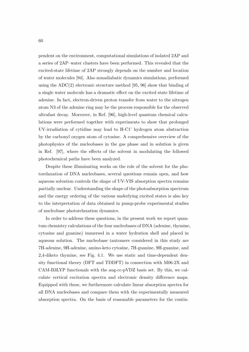
60
pendent on the environment, computational simulations of isolated 2AP and
a series of 2AP–water clusters have been performed. This revealed that the
excited-state lifetime of 2AP strongly depends on the number and location
of water molecules [94]. Also nonadiabatic dynamics simulations, performed
using the ADC(2) electronic structure method [95, 96] show that binding of
a single water molecule has a dramatic effect on the excited state lifetime of
adenine. In fact, electron-driven proton transfer from water to the nitrogen
atom N3 of the adenine ring may be the process responsible for the observed
ultrafast decay. Moreover, in Ref. [96], high-level quantum chemical calcu-
lations were performed together with experiments to show that prolonged
UV-irradiation of cytidine may lead to H-C1’ hydrogen atom abstraction
by the carbonyl oxygen atom of cytosine. A comprehensive overview of the
photophysics of the nucleobases in the gas phase and in solution is given
in Ref. [97], where the effects of the solvent in modulating the followed
photochemical paths have been analyzed.
Despite these illuminating works on the role of the solvent for the pho-
torelaxation of DNA nucleobases, several questions remain open, and how
aqueous solvation controls the shape of UV-VIS absorption spectra remains
partially unclear. Understanding the shape of the photoabsorption spectrum
and the energy ordering of the various underlying excited states is also key
to the interpretation of data obtained in pump-probe experimental studies
of nucleobase photorelaxation dynamics.
In order to address these questions, in the present work we report quan-
tum chemistry calculations of the four nucleobases of DNA (adenine, thymine,
cytosine and guanine) immersed in a water hydration shell and placed in
aqueous solution. The nucleobase tautomers considered in this study are
7H-adenine, 9H-adenine, amino-keto cytosine, 7H-guanine, 9H-guanine, and
2,4-diketo thymine, see Fig. 4.1. We use static and time-dependent den-
sity functional theory (DFT and TDDFT) in connection with M06-2X and
CAM-B3LYP functionals with the aug-cc-pVDZ basis set. By this, we cal-
culate vertical excitation spectra and electronic density difference maps.
Equipped with these, we furthermore calculate linear absorption spectra for
all DNA nucleobases and compare them with the experimentally measured
absorption spectra. On the basis of reasonable parameters for the contin-

61
uous solvent (water), no further fitting parameter enters the calculations.
Apart from a systematic constant energy shift, we find a good agreement
between theoretical and experimental results. A high level of realism in
the calculations is ensured by including several phenomena which affect the
shapes of the absorption spectra (interaction with explicit solvent molecules
through hydrogen bonding, the presence of bulk solvent, tautomeric equilib-
ria, and vibrational broadening) in the simulations. This study is the first to
attempt to systematically reproduce the observed photoabsorption spectra
of all four nucleobases of DNA in aqueous solution.
Figure 4.1: Lewis structures of the tautomers considered in this work.

62
4.1 Electronic structure methods
The quantum chemistry simulations were performed using the static and
time-dependent density functional theory (DFT and TDDFT) methods as
implemented in the computational chemistry software package Gaussian 09,
Revision A.02 [61]. In particular, we have used the M06-2X and CAM-
B3LYP functionals for the TDDFT calculations with the aug-cc-pVDZ ba-
sis set. These functionals have been chosen for the present study because
they are known to perform reasonably well in the context of linear response
TDDFT calculations for molecular clusters. In particular, they do not tend
to underestimate the energies of the states involved in charge-transfer tran-
sitions, and neither do they predict spurious charge-transfer transitions to
occur at low energies [62, 98, 99].
The key new ingredient in this work is the explicit inclusion of a hydra-
tion shell of water molecule around the bases. Simulations of the photoab-
sorption spectra in the UV-VIS range were performed for these microsol-
vated base molecules. For this, clusters of bases and several solvating water
molecules were constructed. The solvation shell around each nucleobase
molecule was constructed in such a way as to saturate all, or most, hy-
drogen bonding sites of the nucleobase, while using as few water molecules
as possible in order to reduce the cost of the computation. For 7H- and
9H-adenine, the structure of the solvation shell was adapted from Ref. [93].
Typically, from five to eight water molecules were included in the investi-
gated geometrical structures.
The interaction of the base molecule and the surrounding explicit wa-
ter molecules with the bulk water solvent was modeled by the continuous
surface charge implementation of the polarizable continuum model (CSC-
PCM) [100, 101]. It was imposed both at the stage of the optimization of
the molecular geometry and in the subsequent simulations of the photoab-
sorption spectra. Linear response solvation was applied in all TDDFT cal-
culations of vertical excitation energies. A dielectric constant of ε = 78.3553
was used for the aqueous solvent. As per default, the solute cavity was con-
structed as a set of overlapping spheres centered at the solute atoms, using
the universal force field atomic radii scaled by a factor of 1.100.

63
Concerning the tautomeric equilibrium state, the population of the 7H-
tautomer of adenine in aqueous solution was assumed to be 22%, as de-
termined experimentally by Cohen et al. [102]. In turn, the population of
the 7H-tautomer of guanine in aqueous solution was taken to be 18%, as
estimated by Yu et al. [103] on the basis of density functional theory (DFT)
calculations. In the cases of cytosine and thymine, only the predominant
tautomers were taken into account (which is to say, amino-keto cytosine and
2,4-diketo thymine).
The semiclassical nuclear ensemble method of Crespo-Otero and Barbatti
[56] has been already described in details in Section 3.2 and has been applied
to model the UV-VIS absorption spectra.

64
4.2 Results and discussion
4.2.1 Equilibrium geometries
Figure 4.2: Equilibrium geometry of the six investigated nucleobase tau-
tomers optimized at the M06-2X/aug-cc-pVDZ level of theory. The lengths
of hydrogen bonds are marked in units of A.

65
Fig. 4.2 shows the optimized geometries and hydrogen bond lengths (in
A) of the six tautomers of microsolvated bases: 7H- and 9H-adenine, cyto-
sine, 7H-keto and 9H-keto tautomers of guanine and thymine.
The O-H bonds have in general a length of approximately 1.9 A.
4.2.2 Calculated vertical excitation spectra
Table 4.1: Vertical excitation spectra (M06-2X/aug-cc-pVDZ) for 7H-
adenine, 9H-adenine and cytosine
Tautomer Electronic state Gas phase PCM solvent model Explicit waters
∆E, eV f ∆E, eV f ∆E, eV f
7H-adenine La1ππ∗ 5.259 0.138 5.182 0.244 5.132 0.315
Lb1ππ∗ 5.810 0.029 5.661 0.048 5.540 0.070
1 1nπ∗ 5.057 0.008 5.415 0.004 5.805 0.001
2 1nπ∗ 5.650 0.001 5.864 0.001 6.191 0.001
1 1πσ∗ 5.146 0.016 5.650 0.008 5.710 0.004
2 1πσ∗ 6.053 0.002 6.304 0.013 6.231 0.001
9H-adenine La1ππ∗ 5.347 0.287 5.271 0.361 5.190 0.410
Lb1ππ∗ 5.523 0.014 5.476 0.027 5.395 0.040
1 1nπ∗ 5.315 0.001 5.447 0.001 5.804 < 10−3
2 1nπ∗ 5.878 0.002 5.984 0.002 6.303 0.001
1 1πσ∗ 5.452 0.007 5.594 0.007 5.658 0.004
2 1πσ∗ 5.731 0.001 6.136 0.001 6.199 0.001
cytosine 1 1ππ∗ 4.974 0.068 5.106 0.125 5.201 0.192
2 1ππ∗ 5.904 0.125 5.906 0.193 5.948 0.098
1 1nπ∗ 5.264 0.002 5.660 0.003 6.028 0.049
2 1nπ∗ 6.334 < 10−3 6.137 < 10−3 6.588 0.004
1 1πσ∗ 5.495 0.004 5.926 0.005 6.130 0.004
2 1πσ∗ 6.100 0.010 6.403 0.002 6.604 0.004
a A valence-to-valence excited state with an admixture of Rydberg character.
Vertical excitation spectra of nucleobase molecules, calculated by using
the TDDFT method at the M06-2X/aug-cc-pVDZ and CAM-B3LYP/aug-

66
Table 4.2: Vertical excitation spectra (M06-2X/aug-cc-pVDZ) for 7H-
guanine, 9H-guanine and thymine
Tautomer Electronic state Gas phase PCM solvent model Explicit waters
∆E, eV f ∆E, eV f ∆E, eV f
7H-guanine La1ππ∗ 4.958 0.132 4.870 0.183 4.684 0.203
Lb1ππ∗ 5.793 0.181 5.373 0.001 5.675 0.297
1 1nπ∗ 5.362 < 10−3 5.511 < 10−3 5.870 < 10−3
2 1nπ∗ 6.137 0.001 6.363 0.001 6.510 0.004
1 1πσ∗ 5.180 0.006 5.738 0.255 5.364 0.002
2 1πσ∗ 5.454 0.009 5.825 0.037 5.941 0.005
9H-guanine La1ππ∗ 5.162 0.136 5.076 0.174 4.921 0.200
Lb1ππ∗ 5.588 0.318 5.490 0.457 5.487 5.486
1 1nπ∗ 5.376 0.002 5.595 < 10−3 5.836 < 10−3
2 1nπ∗ 6.276 0.005 6.412 0.001 6.488 0.002
1 1πσ∗ 4.987 0.016 5.287 < 10−3 5.289 0.004
2 1πσ∗ 5.339 0.010 5.812 0.011 5.889 0.001
thymine 1 1ππ∗ 5.246 0.179 5.156 0.232 5.124 0.239
2 1ππ∗ 6.610 0.108 6.450 0.250 6.310 0.267
1 1nπ∗ 4.971 < 10−3 5.178 < 10−3 5.371 < 10−3
2 1nπ∗ 6.251 < 10−3 6.402 < 10−3 6.605 0.001
1 1πσ∗ 5.633 0.001 5.948 0.001 6.076 0.002
2 1πσ∗ 6.373 0.001 6.497 0.001 6.631 0.002
a A valence-to-valence excited state with an admixture of Rydberg character.
cc-pVDZ levels of theory, are characterized in Tables 4.1, 4.2, 4.3 and 4.4.
Vertical excitation energies (∆E) and associated oscillator strengths (f)
into the low-lying singlet excited states of the six investigated nucleobase
tautomers at their ground-state equilibrium (S0-min) geometries are listed.
Different microenvironments were imposed in the calculations of the verti-
cal excitation spectra: the gas phase, aqueous solvation represented using
both explicit water molecules and the PCM solvation model, and aqueous
solvation represented by only the PCM solvation model. The ππ∗ states are
labeled as La and Lb according to the formalism described in Ref. [16], and

67
Table 4.3: Vertical excitation spectra (CAM-B3LYP/aug-cc-pVDZ) for 7H-
adenine, 9H-adenine and cytosine
Tautomer Electronic state Gas phase PCM solvent model Explicit waters
∆E, eV f ∆E, eV f ∆E, eV f
7H-adenine La1ππ∗ 5.191 0.077 5.133 0.227 5.103 0.292
Lb1ππ∗ 5.734 0.031 5.598 0.053 5.497 0.077
1 1nπ∗ 5.129 0.046 5.504 0.003 5.872 0.001
2 1nπ∗ 5.658 0.002 5.913 0.001 6.241 < 10−3
1 1πσ∗ 5.236 0.033 5.771 0.009 5.904 0.006
2 1πσ∗ 6.166 0.002 6.473 0.002 6.429 0.001
9H-adenine La1ππ∗ 5.316 0.278 5.246 0.349 5.182 0.402
Lb1ππ∗ 5.459 0.012 5.416 0.025 5.341 0.037
1 1nπ∗ 5.339 0.001 5.491 0.001 5.867 < 10−3
2 1nπ∗ 5.916 0.001 6.044 0.002 6.372 0.001
1 1πσ∗ 5.629 0.010 5.764 0.010 5.879 0.005
2 1πσ∗ 5.945 0.003 6.330 0.001 6.427 0.039
cytosine 1 1ππ∗ 4.936 0.064 5.085 0.117 5.196 0.183
2 1ππ∗ 5.870 0.122 5.89 0.190 5.960 0.130
1 1nπ∗ 5.281 0.002 5.695 0.003 6.062 0.025
2 1nπ∗ 5.862 < 10−3 6.255 < 10−3 6.713 0.030
1 1πσ∗ 5.621 0.005 6.058 0.006 6.296 0.006
2 1πσ∗ 6.130 0.003 6.506 0.003 6.752 0.019
a A valence-to-valence excited state with an admixture of Rydberg character.
in agreement with the results presented in Refs. [104], [105].
As the simulated photoabsorption spectra of nucleobases in aqueous so-
lution will be dominated by excitations into the bright excited states of the
majority tautomers, it is of interest to assess the accuracy of the TDDFT
method in combination with the M06-2X and CAM-B3LYP functionals for
the vertical excitations of these states. In order to take advantage of the
most accurate theoretical benchmarks available, the subject of this assess-
ment must be the vertical excitation spectra of the isolated molecules. The
study of Szalay and coworkers [106], which employed coupled cluster meth-

68
Table 4.4: Vertical excitation spectra (CAM-B3LYP/aug-cc-pVDZ) for 7H-
guanine, 9H-guanine and thymine
Tautomer Electronic state Gas phase PCM solvent model Explicit waters
∆E, eV f ∆E, eV f ∆E, eV f
7H-guanine La1ππ∗ 4.887 0.132 4.802 0.182 4.646 0.201
Lb1ππ∗ 5.759 a 0.150 5.720 0.248 6.271 0.382
1 1nπ∗ 5.440 < 10−3 5.608 < 10−3 5.970 < 10−3
2 1nπ∗ 6.039 < 10−3 6.278 0.001 6.455 0.002
1 1πσ∗ 5.292 0.006 5.523 0.001 5.607 0.010
2 1πσ∗ 5.601 0.016 5.960 0.010 5.690 0.254
9H-guanine La1ππ∗ 5.072 0.117 5.015 0.173 4.880 0.197
Lb1ππ∗ 5.559 0.273 5.464 0.440 5.484 0.373
1 1nπ∗ 5.526 0.012 5.741 < 10−3 5.976 < 10−3
2 1nπ∗ 6.324 0.002 6.422 0.002 6.485 0.003
1 1πσ∗ 5.164 0.037 5.452 0.007 5.542 0.055
2 1πσ∗ 5.508 0.044 5.974 0.011 6.140 0.001
thymine 1 1ππ∗ 5.208 0.174 5.122 0.227 5.088 0.234
2 1ππ∗ 6.581 0.046 6.432 0.261 6.293 0.272
1 1nπ∗ 5.082 < 10−3 5.301 < 10−3 5.501 < 10−3
2 1nπ∗ 6.366 < 10−3 6.517 < 10−3 6.724 0.002
1 1πσ∗ 5.775 0.001 6.110 0.001 6.271 0.002
2 1πσ∗ 6.541 < 10−3 6.661 0.001 6.834 0.003
a A valence-to-valence excited state with an admixture of Rydberg character.
ods, is the theoretically most advanced calculation of the vertical excitation
spectra performed to date, and so we use it as a benchmark against which
to compare the results of the TDDFT calculations. In Table 4.5, we com-
pare the vertical excitation energies oscillator strengths of the bright excited
states of nucleobases obtained from the TDDFT calculations with the values
reported in the work just cited. (For our purposes, excited states character-
ized by values of the oscillator strength greater than 0.05 were considered
to be bright.)
It can be seen from Table 4.5 that the TDDFT calculations in combi-

69
M06-2X/aug-cc-pVDZ
Nucleobase Excited state ∆E, eV f
9H-adenine La ππ∗ 5.348 0.2867
cytosine ππ∗ 4.974 0.0687
9H-guanine La ππ∗ 5.163 0.1356
Lb ππ∗ 5.589 0.3174
Thymine ππ∗ 5.246 0.1793
CAM-B3LYP/aug-cc-pVDZ
Nucleobase Excited state ∆E, eV f
9H-adenine La ππ∗ 5.316 0.2783
cytosine ππ∗ 4.936 0.0635
9H-guanine La ππ∗ 5.072 0.1164
Lb ππ∗ 5.559 0.2729
Thymine ππ∗ 5.207 0.1744
EOMEE-CCSD(T)/aug-cc-pVTZ
Nucleobase Excited state ∆E, eV f a
9H-adenine La ππ∗ 5.23 0.275
cytosine ππ∗ 4.69 0.066
9H-guanine La ππ∗ 4.86 0.160
Lb ππ∗ 5.37 0.366
Thymine ππ∗ 5.15 0.213a The values of the oscillator strength are taken from calculations at the
EOMEE-CCSD/aug-cc-pVTZ level of theory.
Table 4.5: Comparison of vertical excitation spectra of the isolated nucle-
obase molecules calculated using the TDDFT method with the use of the
M06-2X and CAM-B3LYP functionals with the benchmark provided by the
EOMEE-CCSD(T) method [106].
nation with either functional systematically overestimate the vertical ex-
citation energies into the bright excited states of nucleobases by up to
around 0.3 eV, in comparison to the benchmark provided by the method

70
of the equation of motion excitation energy coupled-cluster with perturba-
tive triple excitations (EOMEE-CCSD(T)). The exception is thymine, for
which the excitation energies calculated with TDDFT coincide closely with
those obtained at the EOMEE-CCSD(T) level. Therefore, insofar as the
EOMEE-CCSD(T) level of theory can be considered a realistic benchmark
for vertical excitation energies, and assuming this systematic blue shift is
not compensated for by another source of error, we may expect that the
photoabsorption spectra of nucleobases in aqueous solution simulated with
the use of TDDFT, with the M06-2X or the CAM-B3LYP functional, will
exhibit a blue shift of a few tenths of an electronvolt relative to experiment.
Inspection of the data in Tables 4.1-4.4 reveals that aqueous solvation
has a strong influence on the vertical excitation spectra. Across all nucle-
obase molecules considered presently, the participation of the lone electron
pairs in hydrogen bonding with explicit solvating water molecules increases
the vertical excitation energies into the nπ∗-type excited states by a few
tenths of an electronvolt. Meanwhile, the excitation energies into the lowest
ππ∗-type states are shifted downwards by up to around 0.3 eV. The ex-
ception is cytosine, in which the inclusion of explicit solvent molecules and
continuum bulk solvent has the effect of increasing the excitation energy of
the lowest ππ∗ state by roughly 0.2 eV, according to both the M06-2X and
CAM-B3LYP functionals. As a consequence, for each of the microsolvated
nucleobase molecules in continuum aqueous solvent (including cytosine), the
lowest vertical excitation is into a ππ∗-type state, which is energetically sep-
arated from the lowest nπ∗- and Rydberg-type excited states.
This is in contrast to the cases of nucleobases in the gas phase, and with
continuum solvation without the use of explicit solvent molecules, where the
energies of the lowest nπ∗- and ππ∗-type states are comparable.
Moreover, for all six nucleobase tautomers, aqueous solvation also has
the effect of shifting upwards by a few tenths of an electronovolt the exci-
tation energies into the lowest Rydberg-type (πσ∗) excited states. This is
true whether the solvent is modeled using only the CSC-PCM model, or the
CSC-PCM model in combination with explicit water molecules.
The phenomenon whereby the excitation energies into the Rydberg-type
states of a chromophore are increased by the presence of explicit solvent

71
molecules, or substituents bonded to the chromophore, was apparently first
considered by Szalay and coworkers [107], who attributed it to the spa-
tial overlap between the Rydberg-type orbitals of the chromophore and the
orbitals of the nearby chemical moieties. As seen in Tables 4.1-4.4, the
Rydberg-type excited states are also destabilized by interaction with an
implicitly included environment alone, although due to their abstracted na-
ture, the CSC-PCM model provides only a very simplistic description of the
interaction of the Rydberg-type states with the surroundings of the chro-
mophore. The treatment of the Rydberg-type states could in principle be
improved through the further build-up of the explicit solvation shell, but
this approach is unattractive because the simulation cost increases rapidly
with system size.
We note that for the purposes of the present study, however, a highly re-
alistic description of the Rydberg-type excited states is not essential. This
is because, in the absence of mixing with valence-to-valence excited states,
the oscillator strengths of the Rydberg-type excited states are typically of
the order of 0.005, much lower than the oscillator strengths of the low-lying
bright ππ∗-type states, which are in the range of roughly 0.2 to 0.4. It fol-
lows that, according to Eq. 3.13, as long as the number of Rydberg-type
excited states found near the low-lying ππ∗-type states is low, the magni-
tude of the relative error in the calculated photoabsorption coefficient due
to the simplified treatment of the Rydberg-type excited states is therefore
unlikely to exceed 0.005/0.2 = 2.5%.

72
Electron density difference maps (EDDMs)
(a) S1 (La ππ∗) (b) S2 (Lb ππ
∗)
(c) S3 (Rydberg) (d) S4 (nπ∗)
Figure 4.3: EDDMs calculated for the lowest excited states of microsolvated
7H-adenine, calculated at the M06-2X/aug-cc-pVDZ level of theory, and
plotted in the form of isosurfaces with isovalues of ±0.005 e/a03. For each
excited state, the red and blue isosurfaces delimit regions in which the elec-
tron density is increased and decreased, respectively, relative to the singlet
ground state.
Electron density difference maps (EDDMs) have been derived for the six
investigated nucleobase tautomers: 7H- and 9H-adenine, cytosine, 7H- and
9H-keto guanine and thymine. They represent the difference of the electron
density of the excited state and the one of the ground state for a given
molecular geometry, and they are useful to visualize the nature of an excited
electronic state and the orbitals involved in the observed transitions. In

73
Figs. 4.3-4.8, EDDMs are shown for all the investigated molecules. EDDMs
are plotted in the form of isosurfaces with isovalues of ±0.005 e/a03. For
each excited state, the red and blue isosurfaces delimit regions in which
the electron density is increased and decreased, respectively, relative to the
singlet ground state.
(a) S1 (La ππ∗) (b) S2 (Lb ππ
∗)
(c) S3 (Rydberg) (d) S4 (nπ∗)
Figure 4.4: EDDMs calculated for the lowest excited states of microsolvated
9H-adenine, calculated at the M06-2X/aug-cc-pVDZ level of theory, and
plotted in the form of isosurfaces with isovalues of ±0.005 e/a03.

74
(a) S1 (ππ∗) (b) S2 (nπ∗)
(c) S3 (nπ∗) (d) S4 (Rydberg)
Figure 4.5: EDDMs calculated for the lowest excited states of microsolvated
cytosine, calculated at the M06-2X/aug-cc-pVDZ level of theory, and plotted
in the form of isosurfaces with isovalues of ±0.005 e/a03.

75
(a) S1 (La ππ∗) (b) S2 (Rydberg)
(c) S3 (Lb ππ∗) (d) S4 (nπ∗)
Figure 4.6: EDDMs calculated for the lowest excited states of microsolvated
7H−keto guanine, calculated at the M06-2X/aug-cc-pVDZ level of theory,
and plotted in the form of isosurfaces with isovalues of ±0.005 e/a03.
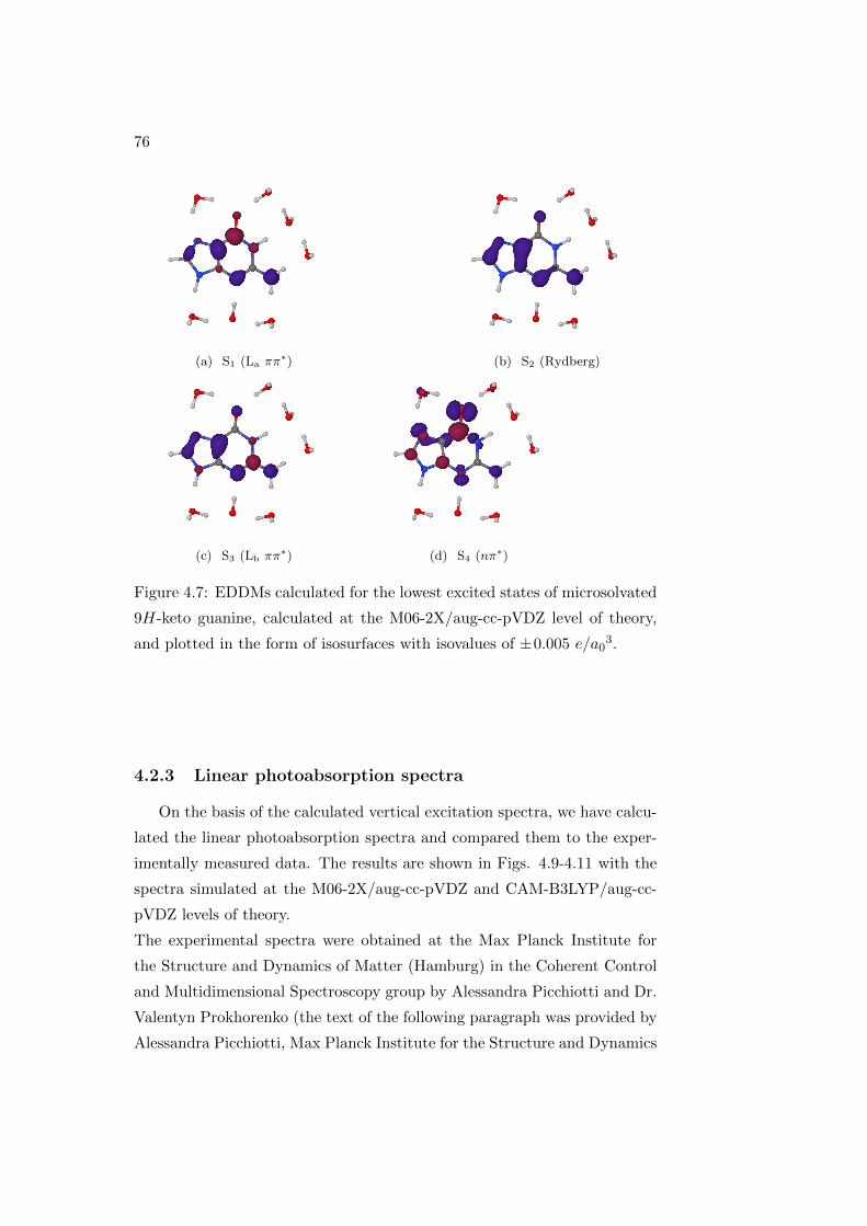
76
(a) S1 (La ππ∗) (b) S2 (Rydberg)
(c) S3 (Lb ππ∗) (d) S4 (nπ∗)
Figure 4.7: EDDMs calculated for the lowest excited states of microsolvated
9H-keto guanine, calculated at the M06-2X/aug-cc-pVDZ level of theory,
and plotted in the form of isosurfaces with isovalues of ±0.005 e/a03.
4.2.3 Linear photoabsorption spectra
On the basis of the calculated vertical excitation spectra, we have calcu-
lated the linear photoabsorption spectra and compared them to the exper-
imentally measured data. The results are shown in Figs. 4.9-4.11 with the
spectra simulated at the M06-2X/aug-cc-pVDZ and CAM-B3LYP/aug-cc-
pVDZ levels of theory.
The experimental spectra were obtained at the Max Planck Institute for
the Structure and Dynamics of Matter (Hamburg) in the Coherent Control
and Multidimensional Spectroscopy group by Alessandra Picchiotti and Dr.
Valentyn Prokhorenko (the text of the following paragraph was provided by
Alessandra Picchiotti, Max Planck Institute for the Structure and Dynamics
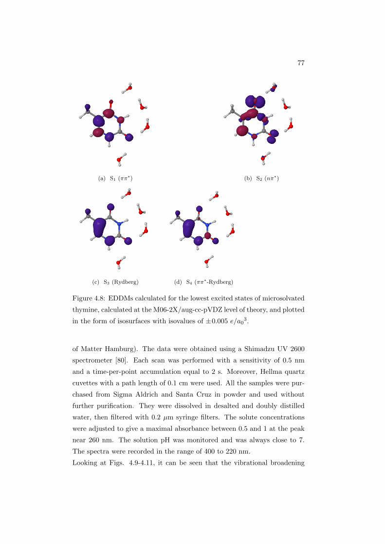
77
(a) S1 (ππ∗) (b) S2 (nπ∗)
(c) S3 (Rydberg) (d) S4 (ππ∗-Rydberg)
Figure 4.8: EDDMs calculated for the lowest excited states of microsolvated
thymine, calculated at the M06-2X/aug-cc-pVDZ level of theory, and plotted
in the form of isosurfaces with isovalues of ±0.005 e/a03.
of Matter Hamburg). The data were obtained using a Shimadzu UV 2600
spectrometer [80]. Each scan was performed with a sensitivity of 0.5 nm
and a time-per-point accumulation equal to 2 s. Moreover, Hellma quartz
cuvettes with a path length of 0.1 cm were used. All the samples were pur-
chased from Sigma Aldrich and Santa Cruz in powder and used without
further purification. They were dissolved in desalted and doubly distilled
water, then filtered with 0.2 µm syringe filters. The solute concentrations
were adjusted to give a maximal absorbance between 0.5 and 1 at the peak
near 260 nm. The solution pH was monitored and was always close to 7.
The spectra were recorded in the range of 400 to 220 nm.
Looking at Figs. 4.9-4.11, it can be seen that the vibrational broadening

78
shifts the simulated spectra to the red relative to the vertical excitation spec-
trum calculated for the ground-state equilibrium geometry. We note that
both for 7H-adenine and 9H-adenine, and for 7H-guanine and 9H-guanine,
a weighted sum of the spectra is shown in order to obtain a more realistic
absorption spectrum containing both tautomers.
In general, the form of the experimental spectra in the low-energy regime
is well reproduced by the simulations. All calculated spectra are blue-shifted
relative to the experimental data by approximately 0.3 eV. The systematic
shifts of the peaks of the two lowest bands between the experimental and
simulated spectra are collected in Tables 4.6 and 4.7, together with the rel-
ative error of the photoabsorption cross section. This quantity has been
determined according to the relation (see Fig. 4.12 for a graphical explana-
tion)
∆σ
σ=σcalcmax − σobsmax
σobsmax. (4.1)
In the case of cytosine, the second peak in the experimental spectrum is
outside the range of 3.50 to 6.20 eV in which the data were collected. For
this reason, we could not analyze the corresponding error in the position
and intensity of the second peak in this case.
The chosen basis set aug-cc-pVDZ is moderately large, but from a com-
putational point of view, an even larger basis could be chosen. Therefore,
to investigate the effect of using a larger one, we have also used the basis set
aug-cc-pVTZ. The importance of this effect is estimated by re-optimizing the
geometries of the six nucleobase-water clusters at the M06-2X/aug-cc-pVTZ
and CAM-B3LYP/aug-cc-pVTZ levels of theory, and then re-calculating
their vertical excitation spectra for the resulting geometries. The compari-
son between the stick spectra calculated by using aug-cc-pVDZ and aug-cc-
pVTZ is presented in Figs. 4.13 and 4.14, where the stick spectra of the two
levels of theory are superposed.
Somewhat counter-intuitively, the vertical excitation energies for the low-
lying bright states generally increase slightly when the calculation is repeated
with the larger aug-cc-pVTZ basis set at the re-optimized energy. In fact, it
would be normally expected that the blue shift is reduced and the excitation

79
Figure 4.9: Simulated absorption spectra of nucleobases in aqueous solu-
tion, computed at the M06-2X/aug-cc-pVDZ level of theory, compared to
the experimentally observed (experimental data by courtesy of Alessandra
Picchiotti, Max Planck Institute for the Structure and Dynamics of Mat-
ter Hamburg) spectra. The black columns indicate the vertical excitation
energies evaluated at the ground-state equilibrium geometry, and their rel-
ative heights are proportional to the corresponding oscillator strengths. In
the case of adenine and guanine, the spectra are averaged over the 7H- and
9H- tautomers of both bases according to their populations, and the column
heights are also scaled proportionally to the respective populations.

80
Figure 4.10: Simulated absorption spectra of nucleobases in aqueous solu-
tion, computed at the CAMB3LYP/aug-cc-pVDZ level of theory, compared
to the experimentally observed (experimental data by courtesy of Alessandra
Picchiotti, Max Planck Institute for the Structure and Dynamics of Mat-
ter Hamburg) spectra. The black columns indicate the vertical excitation
energies evaluated at the ground-state equilibrium geometry, and their rel-
ative heights are proportional to the corresponding oscillator strengths. In
the case of adenine and guanine, the spectra are averaged over the 7H- and
9H- tautomers of both bases according to their populations, and the column
heights are also scaled proportionally to the respective populations.

81
Figure 4.11: Comparison of photoabsorption spectra for the four DNA nucle-
obases simulated using the M06-2X and the CAM-B3LYP functionals with
the experimentally observed (experimental data by courtesy of Alessandra
Picchiotti, Max Planck Institute for the Structure and Dynamics of Matter
Hamburg) spectra.

82
Figure 4.12: Graphical explanation of calculation of values in Tabs. 4.6 and
4.7.

83
Nucleobase Ecalcmax1, eV shift in Ecalc
max1, eV ∆σ/σ at max1
adenine 5.050 0.291 −0.0481
cytosine 5.010 0.358 0.0855
guanine 4.830 0.304 0.0678
thymine 4.970 0.283 −0.0286
Nucleobase Ecalcmax2, eV shift in Ecalc
max2, eV ∆σ/σ at max2
adenine 6.350 0.360 −0.113
cytosine
guanine 5.350 0.332 0.052
thymine 6.280 0.247 −0.204
Table 4.6: Systematic shifts of the peaks and relative errors of the photoab-
sorption cross section of the lowest (max1) and the second lowest (max2)
band between experimental and simulated spectra for the four DNA nucle-
obases, from calculations performed using the M06-2X functional.
Nucleobase Ecalcmax1, eV shift in Ecalc
max1, eV ∆σ/σ at max1
adenine 5.010 0.251 −0.043
cytosine 5.020 0.368 0.0549
guanine 4.810 0.274 0.054
thymine 4.890 0.203 −0.009
Nucleobase Ecalcmax2, eV shift in Ecalc
max2, eV ∆σ/σ at max2
adenine 6.300 0.310 −0.071
cytosine
guanine 5.320 0.302 −0.032
thymine 6.470 0.438 −0.156
Table 4.7: Same as Table 4.4, but using the CAM-B3LYP functional.

84
Figure 4.13: Simulated stick spectra for the six DNA nucleobases tautomers
derived from the M06-2X calculation: comparison between results obtained
by using the aug-cc-pVDZ (black) and aug-cc-pVTZ (red) basis sets.

85
Figure 4.14: Simulated stick spectra for the six DNA nucleobases tau-
tomers derived from CAM-B3LYP calculation: comparison between results
obtained by using the aug-cc-pVDZ (black) and aug-cc-pVTZ (red) basis
sets.

86
energies decrease with increasing the basis set size. Yet, we find that the
vertical excitation energy to the lower bright state are only slightly affected
by enlarging the basis set.
In general, the spectra of the four nucleobases are composed of two clearly
visible bands, separated by a low intensity region. In the case of adenine
and thymine, each of these bands is due to a single bright ππ∗ transition.
For guanine, four ππ∗ states contribute to the lowest photoabsorption band,
i.e., the excitations into the lowest two ππ∗ states arise (the La and Lb states
of each tautomer). This may be related to multiple decay pathways which
can be identified in the molecule after UV absorption [57].
Regarding cytosine, there has been a debate in previous studies as to how
many bright excited states give significant contributions to the photoabsorp-
tion spectrum. On the basis of the linear vibronic coupling method and on
the equations-of-motion coupled cluster with single and double excitations
(EOM-CCSD) level of electronic structure theory, Tajti et al. [108] have
performed spectral simulations for cytosine in the gas phase. They have in-
terpreted the resulting photoabsorption spectrum up to around 60000 cm−1
(7.4 eV) as arising mainly from transitions to only two ππ∗-type states.
Subsequently, Barbatti and coworkers [57] have demonstrated that a third
ππ∗-type state must be taken into account in order to explain the appearance
of the gas-phase spectrum. The present results for microsolvated cytosine in
a bulk solvent indicate that in aqueous solution the number of excited elec-
tronic states which significantly contribute to the photoabsorption spectrum
is even higher. This is due to a mixing of ππ∗ and nπ∗ states. This is fur-
ther supported by the the EDDMs of the low-lying excited electronic states
of microsolvated cytosine calculated at the M06-2X/aug-cc-pVDZ level at
the ground-state equilibrium geometry, which are shown in Fig. 4.5. The
S2 and S3 states are both nominally nπ∗ in character, but also involve a
substantial redistribution of the π-type electron density. These nπ∗ states
have a sizable admixture of ππ∗ character which is reflected by their mod-
erately large oscillator strengths (0.098 and 0.049, respectively, for S2 and
S3). The contribution of these nπ∗ states to the photoabsorption spectrum
is mainly significant in the interband region around 5.5 eV in the simulated
spectrum. This feature may trigger different deactivation pathways right

87
after the photoabsorption [57].
Cytosine has the largest shift between the experimental and calculated spec-
tra for both the functionals M06-2X and CAM-B3LYP. The peak in the
simulated spectra is in the valley of the experimental spectrum, see Figs.
4.9-4.11. The effect of the explicit inclusion of the water molecules form-
ing the hydration shell seems to play a quite important role in particular
for cytosine. To study this in more detail, we have simulated the pho-
toabsorption spectra of cytosine with the polarizable continuum model but
without explicitly including the water molecules of the hydration shell, at
the CAM-B3LYP/aug-cc-pVDZ and M06-2X/aug-cc-pVDZ levels of theory.
The results for the photoabsorption spectra are shown in Fig. 4.15. The
general form of these spectra in the presence of a bulk solvent only is sim-
ilar to that when explicit water molecules are additionally included, but,
importantly, the intensity of the first absorption band is significantly un-
derestimated with respect to the experiment. Hence, this indicates that at
least for cytosine, the inclusion of explicit solvent molecules is mandatory in
order to reproduce the experimentally-observed spectrum. A total of four
excited states with vertical excitation energies below 7 eV have significant
oscillator strengths (larger than 0.1).

88
Figure 4.15: Spectrum of cytosine simulated on the level of M062X/aug-cc-
pVDZ and CAM-B3LYP/aug-cc-pVDZ without an explicit hydration shell,
but only bulk solvent taken into account within the polarizable continu-
ous medium (PCM) method (experimental data by courtesy of Alessandra
Picchiotti, Max Planck Institute for the Structure and Dynamics of Matter
Hamburg). The vertical bars indicate the associated stick spectrum .

89
Dependence on line-shape parameter
Figure 4.16: Simulated spectra for cytosine on the level of M062X/aug-cc-
pVDZ and CAM-B3LYP/aug-cc-pVDZ by including bulk solvent within the
PCM method and neglecting explicit microsolvation, changing the δ param-
eter from 0.2 eV to 0.05 eV (experimental data by courtesy of Alessandra
Picchiotti, Max Planck Institute for the Structure and Dynamics of Matter
Hamburg).

90
In the spectral simulations reported in this work, the value of the line-
shape parameter δ, which appears in Eq. (3.15) and which controls the
width of the line-shape function, was set to the relatively large value of
0.2 eV. The reason for this choice is the aim to obtain smooth simulated
spectra to facilitate the comparison with the experiment. With the goal of
understanding the role of the line-shape parameter, we have investigated the
effect of using a smaller value of δ by recalculating the PCM-only spectra
of cytosine without an explicit hydration shell, by setting δ=0.05 eV. The
resulting absorption spectra are shown in Fig. 4.16. We find that the spectra
obtained with the smaller value of δ have a rough and less smooth shape
due to statistical noise in the calculations, but the overall shapes of the
absorption bands are essentially the same as with δ=0.2 eV. Hence, this
justifies the use of the larger value of δ=0.2 eV to obtain a smooth spectrum
which is in fair agreement with the experimental data.
4.3 Conclusions
The photoabsorption spectra of the four canonical DNA nucleobases ex-
plicitly coupled to a hydration shell of water molecules and embedded in
bulk aqueous solution have been simulated using the semiclassical nuclear
ensemble method in combination with the time-dependent density functional
theory and two choices of the exchange-correlation functional (the M06-2X
and CAM-B3LYP functionals). A major difference to existing approaches
is that we have explicitly included a finite number of water molecules in
the simulations which form a hydration shell. We find that the hydration
shell of the microsolvated nucleobases plays an important role. In general,
both functionals reproduce the general form of the experimentally observed
photoabsorption spectra, while at the same time giving rise to a systematic
energy shift in the calculated positions of absorption peaks. Importantly,
we confirm that the M06-2X and CAM-B3LYP functionals do not give rise
to spurious intermolecular charge transfer excited states when the explicitly
solvated nucleobase molecules are considered. Therefore, these function-
als are well suited for the simulation of the photoabsorption spectra, when
hydration shells are included explicitly.

91
Hydrogen bonding with explicit solvent molecules destabilizes the nπ∗-
type excited states of all four nucleobases relative to the low-lying ππ∗-type
excited states. This destabilization will persist following photoexcitation
into the low-lying bright ππ∗-type states for as long as the system remains
near the Franck-Condon geometry, and all hydrogen bonds with the solvat-
ing water molecules are intact. During this period of time, the nπ∗-type
states will therefore be too high in energy to be populated to a significant
extent. It follows that a rearrangement of the solvating water molecules is a
prerequisite for population transfer into the nπ∗-type states. Precisely this
sequence of events was recently predicted to take place in the relaxation dy-
namics of microsolvated 7H-adenine [93]: in this system, the populated state
initially had a pure ππ∗ character, and gradually acquired a mixed ππ∗- and
nπ∗-type character concurrently with a rearrangement of the solvation shell.
The latter process occurred on a timescale of 100-200 fs. Extrapolating to
the other nucleobase molecules in aqueous solution, we therefore expect that
hydrogen bonding with the solvent will generally delay population transfer
into the nπ∗-type at least until some 100-200 fs following the initial pho-
toexcitation.
Moreover, the additional inclusion of vibrational broadening seems essen-
tial for a reliable comparison of simulated photoabsorption spectra with
experimental data, as the peaks in the vibrationally-broadened spectra are
consistently red-shifted with respect to the vertical excitation energies cal-
culated at the ground-state equilibrium geometries. Further spectroscopic
studies in terms of ultrafast 2D spectroscopy is necessary to confirm this
picture. Yet, the present study can serve as a basis for future simulations of
experimental 2D spectra.

92

Chapter 5
2D electronic spectroscopy of
adenine
Adenine is a prominent example of the decay behavior of DNA nucle-
obases, exhibiting ultrafast radiationsless decay and low emission quantum
yields, which has been extensively investigated, but sofar no definite agree-
ment concerning the relaxation mechanism after excitation has been reached.
Recently, the photophysics of nucleobases was experimentally investigated
by means of transient absorption (pump-probe) and 2D spectroscopies [109]
at the Max Planck Institute for the Structure and Dynamics of Matter (Ham-
burg) in the Coherent Control and Multidimensional Spectroscopy group.
As an example, Fig. 5.1 presents experimental pump-probe spectra and 2D
spectrum at T=225 fs for adenine in water.
They found that, in all nucleobases, deactivation of the induced population
occurs via a “dark” state which is presumably the so-called nπ∗ state, popu-
lated from the excited state ππ∗ via conical intersection (CI) between them.
Further decay of the population of the nπ∗ state occurs via the second CI
which connects the nπ∗ and ground states. From the experiments the au-
thors derived a spectroscopic model, shown on Fig. 5.2, which convincingly
explains their observation [109].
In the following we focus our consideration on the dominant 9H-isomer of
adenine. In the first part we present the modeling results of the 2D electronic
spectroscopy, based on phenomenological model (a) (Fig. 5.2) and obtained
93

94
Figure 5.1: Experimental transient absorption (top) and 2D spectra of 9H-
adenine for waiting time T=225 fs (bottom) [109] (experimental data by
courtesy of Alessandra Picchiotti, Max Planck Institute for the Structure
and Dynamics of Matter Hamburg).
by applying the TNL method, which has been introduced in Section 3.3.
In the second part of this Chapter, we will use the exact hierarchy equation
of motion (HEOM) approach to compare calculated 2D electronic spectra

95
Figure 5.2: Spectroscopic model derived from the experiments: phenomeno-
logical (a) and quantum-chemical (b)
with those obtained from the approximate TNL method and with the exper-
imental one. However, the HEOM approach is exact only for a specifically
chosen spectral density of bath states which restricts the modeling to a high
temperature limit. For this modeling we will use the quantum-mechanical
spectroscopic model (b) (Fig. 5.2) which explicitly accounts for two CIs and
also includes a basic vibrational structure for the involved excited states.
5.1 Time Nonlocal Method
5.1.1 Theoretical modeling
Although several excited states play a role in the dynamics of photoex-
cited adenine, and many decay paths are proposed for this molecule, see
Sec. 1.2, we focus here on a minimal kinetic model derived from experimen-
tal results which is schematically shown in Fig. 5.3 (see also panel (a) in
Fig. 5.2) in which the first CI is formally accounted for by introducing a
coupling parameter V between “bright” and “dark” states.

96
Figure 5.3: Phenomenological model for the UV deactivation of 9H-adenine
After the excitation of the molecule from the ground state S0 to the S1
ππ∗ excited state, the deactivation of population to the ground state occurs
directly (weak channel, approximately 40 ps decay) and via a dark nπ∗
state (main channel, approximately 700 fs decay). Two higher excited states
ESA1 and ESA2 contribute to the measured signals due to absorption from
the populated ππ∗ and nπ∗, respectively. µ indicates the transition dipole
moments associated with the excitations to the bright state involved in this
theoretical model and to highly-excited states.
Transient absorption spectroscopy of adenine reveals three decay times: the
shortest is due to the flow of population from the excited to the “dark”
state. The associated decay time is ∼ 0.6 − 0.7 ps. Depopulation of the
dark state occurs via a CI with the ground state S0 within a decay time
of ∼ 1.5 − 1.8 ps. The third channel is the direct population decay to the
ground state from the excited S1 state with a decay time of ∼ 40 ps. In

97
the present modeling these last two decay channels will be accounted for
phenomenologically (see below).
The formalized Hamiltonian belonging to the energy level scheme of Fig.
5.3 is
Hs =
g 0 0 0 0
0 εππ∗ V 0 0
0 V εnπ∗ 0 0
0 0 0 εESAππ∗ 0
0 0 0 0 εESAnπ∗
(5.1)
where εππ∗ = 37600 cm−1 and εnπ∗ = 37150 cm−1 are the energies of the S1
ππ∗ and the dark nπ∗ states, V = 50 cm−1 is the coupling energy between
the two states, εESAππ∗ = 72600 cm−1 and εESAnπ∗71650 cm−1 are the en-
ergies of the two excited state absorption states.
In Subsection 3.3.2 we reviewed the theory of the TNL method. Accord-
ing to this approach, the Liouville equation describing the evolution of the
total system, formed by the system and the bath, is first projected following
the procedure of Nakajima–Zwanzig [67] and then decomposed into a set of
coupled equations for ρs, ρrk(t), ρ
lk(t) which are local in time but still treat
both memory and initial correlations correctly (see Ref. [69])
ρs(t) = Leffs (t)ρs(t) + λ×
(nr∑k=1
αrkL−ρrk(t) +
nl∑k=1
αlkL−ρlk(t)
), (5.2)
ρrk(t) = (Ls(t) + γrk)ρrk(t) + λL−ρs(t) k = 1, nr, (5.3)
ρlk(t) = (Ls(t) + γlk)ρlk(t) + λL+ρs(t) k = 1, nl. (5.4)
This approach can be applied to reproduce the linear and the 2D electronic
spectra of our simplified model for 9H-adenine. The decays of the bright
and dark states to the ground state S0 are not explicitly included in the
TNL model, but their contributions are modeled using a Lindblad equation:
ρ(t) = −i[H, ρ(t)] +M∑k=1
γk
(Lkρ(t)L†k −
1
2L†kLkρ(t)− 1
2ρ(t)L†kLk
)(5.5)

98
5.1.2 Results
The calculated linear absorption spectrum of 9H-adenine is shown in Fig.
5.4. Overlapped in the same plot the experimental absorption and the laser
spectra are shown for comparison.
The spectrum seems to be very narrow as compared to the experimental
one, and this is due to the fact that in the current investigation we’re more
focused on fitting the transient absorption spectra. The model is subject
to improvement, in order to get a satisfactory agreement with experimental
linear absorption spectra. The 2D spectra, calculated for different waiting
Figure 5.4: Theoretical and experimental absorption spectrum of 9H-
adenine, overlapped is the laser spectrum (blue dotted line) (experimen-
tal data by courtesy of Alessandra Picchiotti, Max Planck Institute for the
Structure and Dynamics of Matter Hamburg).
times, are shown in Fig. 5.5. For calculation of this spectrum we used an
infinitely-short laser pulse (impulsive limit in excitation).
Direct comparison with Fig. 5.1 shows good agreement between the
magnitudes and positions of positive and negative peaks in the simulated
and experimental spectra. This is a first confirmation of the reliability of
the spectroscopic model proposed in Ref. [109].
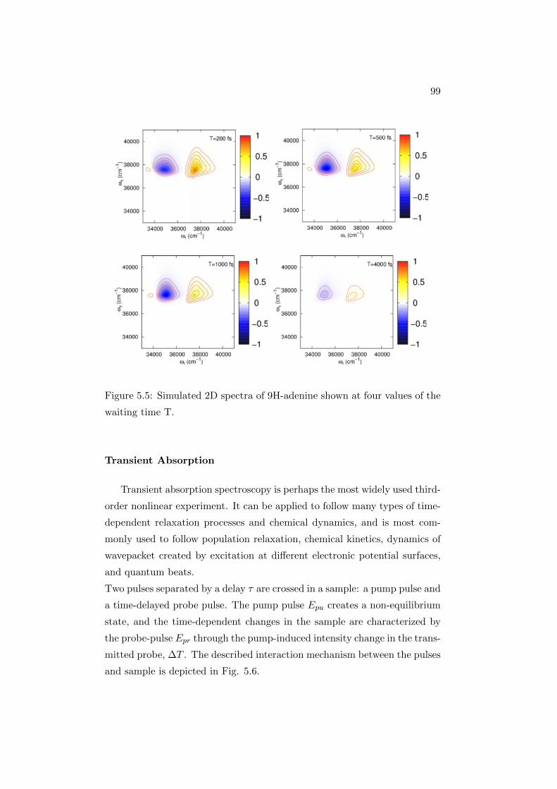
99
Figure 5.5: Simulated 2D spectra of 9H-adenine shown at four values of the
waiting time T.
Transient Absorption
Transient absorption spectroscopy is perhaps the most widely used third-
order nonlinear experiment. It can be applied to follow many types of time-
dependent relaxation processes and chemical dynamics, and is most com-
monly used to follow population relaxation, chemical kinetics, dynamics of
wavepacket created by excitation at different electronic potential surfaces,
and quantum beats.
Two pulses separated by a delay τ are crossed in a sample: a pump pulse and
a time-delayed probe pulse. The pump pulse Epu creates a non-equilibrium
state, and the time-dependent changes in the sample are characterized by
the probe-pulse Epr through the pump-induced intensity change in the trans-
mitted probe, ∆T . The described interaction mechanism between the pulses
and sample is depicted in Fig. 5.6.

100
Figure 5.6: Pump probe setup (picture taken from: Tomakoff Group, Non-
linear and Two dimensional Spectroscopy Notes).
Calculation of the pump-probe (PP) spectra of 9H-adenine was per-
formed according to the method introduced in Ref. [110], briefly reviewed
in the following.
The system’s response to the applied fields
Ea(t) = λaEa(t− τa) exp i(kar− ωat) (5.6)
where λa, ka, ωa and τa denote amplitude, wavevector, frequency and tem-
poral position of the pulses, is determined by the total complex nonlinear

101
polarization
P (r, t) = Tr[µρ(r, t)] (5.7)
which contains contributions corresponding to all possible values of the wave
vector k = l1k1 + l2k2 , with la being arbitrary integers. The pump probe
polarization PPP (t) corresponds to the phase-matching condition l1 = 0,
l2 = 1. PPP (t) can be retrieved from the total polarization P (t) by the
formula
PPP (t) =1
2π
∫ 2π
0dϕ2 exp [−iϕ2]P (ϕ2; t), (5.8)
where P (ϕ2; t) is computed for specific values of the phase angles (k1r = 0
and k2r = ϕ2). Once PPP (t) has been determined, the transient absorption
integral PP signal is obtained according to
SPP (t) = Im
∫ ∞−∞
dtE2(t)(PPP (t)− P offPP (t)), (5.9)
where P offPP (t) is the polarization induced solely by the probe pulse, and
T = τ2 − τ1 is the time delay between the pump and probe pulses.
Pump probe spectra have been simulated for 9H-adenine by applying
the already introduced TNL model.
T (fs)
Wavele
ngth
(nm
)
0 1000 2000 3000 4000 5000
250
260
270
280
290
300 −0.6
−0.4
−0.2
0
0.2
0.4
0.6
0.8
Figure 5.7: Simulated pump-probe spectrum of 9H-adenine

102
0 1000 2000 3000 4000 5000−1
−0.5
0
0.5
1
T (fs)
Am
plit
ude (
arb
.unit)
Theory (266 nm)
Theory (285 nm)
Experiment (266 nm)
Experiment (285 nm)
Figure 5.8: Pump probe amplitude of 9H-adenine (experimental data by
courtesy of Alessandra Picchiotti, Max Planck Institute for the Structure
and Dynamics of Matter Hamburg).
In Fig. 5.7 we show numerically simulated pump-probe spectrum, while
in Fig. 5.8 the experimental and calculated PP traces are overlaid, showing
good agreement between each other. The red and blue lines are the PP
amplitude profiles of the red and the blue peak in the calculated spectra,
respectively. The increasing trend in the PP-amplitude of the blue peaks,
which reflects a decay of ππ∗ state and population growth of nπ∗ state mon-
itored via ESA, is reproduced very well.
From the relatively good agreement between the experimental and numeri-
cal results, we can conclude that the phenomenological model shown in Fig.
5.2 (a) supports the experimental observation and validates our theoretical
model. Moreover, concerning the results already achieved for adenine and
presented in Sec. 1.2, we can conclude that our results of numerical simu-
lation of the PP kinetics supports two of the three decay pathways found
in experiments [109], i.e. the 1Laππ∗ → nπ∗ → S0 and the 1Laππ
∗ → S0
paths.

103
5.2 Hierarchy Equations of Motion
The 2D and pump-probe spectra of adenine in aqueous solution have
been also simulated by applying the second method, the Hierarchy equa-
tions of motion, which was already briefly introduced in Section 3.3.3. This
is a more accurate and precise method and also allows us to take into con-
sideration both CIs explicitly. The signatures of conical intersections have
been detected, and the results obtained from these simulations will be pre-
sented in this section.
Many molecules of interest in spectroscopy exhibit conical intersections
[111]-[118]. Here, we focus in particular on a conical intersection between
the electronic excited state and the ground state, in addition to possible con-
ical intersections between the excited states. Such conical intersections have
been suggested to be present in the nucleobase 9H-adenine (see Section 1.2
and the References listed therein), where they are responsible for ultrafast
deactivation of the excited state. Due to fast dynamics, a rich waiting time
dependence of the two-dimensional spectrum is expected for these systems
[119]-[121]. Of particular interest in this study are the conical intersections
between excited and the ground states.
Nonadiabatic coupling between the excited and ground states was also con-
sidered for a one-dimensional model by Tanimura [79]. In the one-dimensional
model used, a coupling between diabatic states leads to avoided crossing of
the adiabatic surfaces. To go one step further and obtain a conical intersec-
tion of these surfaces, one needs to introduce at least two vibrational modes
[122].
Although several excited states play a role in the wavepacket dynamics of
photoexcited adenine [123], we focus here on a minimal model that cor-
responds to the kinetic model derived from the experimental results and
depicted in Fig. 5.2 (b).
5.2.1 Theoretical modeling
A minimal model for a conical intersection is the linear vibronic cou-
pling model [124, 119]. In this work, we will generalize this model to include
three potential energy surfaces with two CIs: the ground state, a bright

104
Figure 5.9: Diabatic potential energy surfaces along the tuning coordinate
Q2.
ππ∗ state and a dark state, see Fig. 5.9. In addition, as in the previous
modeling, we include the ESA channels for both the bright and the dark
state (not shown). This model differs from the previous one considered in
the framework of TNL by inclusion of a vibronic structure composed by two
vibrational states, which are thought to play an important role in the dy-
namics of the excited states. The present model sketched in Fig. 5.9 includes
both conical intersections CI1 and CI2; however, the direct decay channel
from the excited to the ground state is not accounted for(due to a very long
decay time as compared to the fast deactivation pathways). It should be
noted that, in this model, numerical calculations are limited by the shapes
of potential surfaces: all of them are parabolic (harmonic potentials) and
have the same curvatures.
In this model, three coordinates are involved: the tuning coordinate, along
which the coupling between diabatic states changes, and two coupling coor-
dinates, one for each considered conical intersection. This is a generalization
of the treatment introduced in Chapter 3 (where just one coordinate was
describing both the two CIs), ensuring a more accurate description of the
model.
The potential energy surfaces along the tuning coordinate are harmonic,
105
and the dependence of the diabatic coupling on the coupling coordinate is
linear. This coupling coordinate is not explicitly shown in Fig. 5.9. Ide-
ally, it would be perpendicular to the plane on which the tuning-dependent
potential surfaces are lying. In the present model the tuning and coupling
coordinates have separate and uncorrelated vibrational modes.
Three parabolas represent the three harmonic potentials corresponding
to the ground state S0, the bright ππ∗ and the dark state nπ∗.
The Hamiltonian is given as the sum of a Hamiltonian for the two po-
tential energy surfaces and a Hamiltonian for their coupling to the harmonic
oscillator bath. The first part of the Hamiltonian for three modes is given
by
HP = εe|e〉〈e|+ εd|d〉〈d|
+ M2Ω22Q2deD2|e〉〈e|+M2Ω2
2Q2ddD2|d〉〈d|
+ M1Ω21Q1D1(dV 1|d〉〈e|+ h.c.)
+ M1′Ω21′Q1′D1′(dV 1′ |g〉〈d|+ h.c.), (5.10)
where εe and εd are the vertical transition energies of the ππ∗ state |e〉 and
dark state |d〉, Mj , Dj and Ωj are masses, length scales and frequencies of
the modes with coordinates Qj , and di are the dimensionless displacements.
The potentials for the tuning coordinate Q2 and the coupling coordinates
Q1 and Q1′ are harmonic.
In order to describe damping, we couple the system Hamiltonian to a
bath consisting of infinitely many harmonic oscillators. The interaction of
the coupling and tuning modes with the bath is given by the Hamiltonian:
HSB =∑α
p2α
2mα+
1
2mαω
2α(xα −
g1α
mαω2α
Q1)2
+1
2mαω
2α(xα −
g1′α
mαω2α
Q1′)2
+1
2mαω
2α(xα −
g2α
mαω2α
Q2)2, (5.11)
where mα, ωα, xα and pα are the masses, frequencies, coordinates and mo-
menta of the infinitely many harmonic bath oscillators, and giα are their
coupling strengths to the system.

106
Because of the assumed linear coupling to a harmonic bath, all informa-
tion about the bath and the system bath coupling is encoded in the spectral
densities. The spectral densities are defined as
Ji(ω) =∑α
g2iα
2mαωαδ(ω − ωα), (5.12)
and are chosen to be Ohmic,
J(ω) = Miγiω exp−ω/Λ, (5.13)
where we will take the cut-off Λ larger than all other frequencies in the
system, so that it can be set to infinity. The parameters γi measure the
strength of the damping.
Through a canonical transformation the Hamiltonian is rewritten as [78]
H = εe|e〉〈e|+ εd|d〉〈d|
− (dd|d〉〈d|+ de|e〉〈e|)∑α
g′2αx′α
− (dV 1|d〉〈e|+ h.c.)∑α
g′1αx′α
− (dV 1′ |g〉〈d|+ h.c.)∑α
g′1′αx′α (5.14)
The transformed spectral density, defined for the couplings to the trans-
formed bath g′iα is of the Brownian oscillator form, with reorganization
energies λi = MiD2i Ω
2i /2π~. In the overdamped limit, which allows the
simplest calculation and agrees with experimental results, we approximate
the spectral density by the Debye form
JiOD(ω) = 2λiωc,iω
ω2 + ω2c,i
, (5.15)
where ωc,i is the cut-off frequency.
A hierarchy of equations of motion can be derived by generalizing the
treatment in Refs. [77] and [79] to three coordinates and overdamped baths.
In our calculations, we use the form of the hierarchy proposed in Ref. [125].
Linear spectra, pump-probe spectra and two-dimensional optical spectra can
be calculated with the standard perturbative method. In order to include
induced absorption in the calculation of two-dimensional spectra, we add two

107
levels with energies εf1 and εf2, which can be excited optically from the ππ∗
and dark states, respectively. We do not include dynamics for these states
in the model. Therefore, they are simply characterized by their excitation
energies εf1 and εf2 and transition dipoles µESA1 and µESA2.
5.2.2 Results
In the calculation we used the following set of parameters which allows
satisfactory agreement between the modeled and experimental data: εe =
4.75 eV, εd = 6.3 eV, d2eλ2 = 16 meV, d2
dλ2 = 100 meV, d2V 1λ1 = 9.6 meV,
d2V 1′λ1′ = 4.32 meV, ωc,1 = ωc,1′ = 0.5 eV, ωc,2 = 0.15 eV and εf1 = 8.8 eV,
εf2 = 10.3 eV, µESA1 = 0.7, µππ∗ , µESA2 = 2.0, µππ∗ and β = 0.5/ eV.
In the numerical simulations of 2D and PP spectra horizontal displace-
ments de and dd play a significant role through their product with the reor-
ganization energy λ2, which gives the strength of the coupling to the bath
of the tuning coordinate. The response function formalism with delta (in-
finitely short) laser pulses has been used for the current calculations.
200 220 240 260 280 300 320 340wavelength (nm)
0.0
0.2
0.4
0.6
0.8
1.0
linea
r abs
orption
Figure 5.10: (solid) Calculated and (dashed) experimental linear spectrum
(experimental data by courtesy of Alessandra Picchiotti, Max Planck Insti-
tute for the Structure and Dynamics of Matter Hamburg).
In Fig. 5.10 the calculated and the experimentally obtained linear ab-

108
0 2000 4000time (fs)
0.0
0.2
0.4
0.6
0.8
1.0po
pulatio
n
Figure 5.11: Dynamics of a system with two conical intersections. Plotted
are the populations of the diabatic states. Color coding is as in the potential
energy surfaces in figure 5.9.
sorption spectra are overlaid: by comparing with Fig. 5.4 we can see a
much better performance of the HEOM method with respect to the TNL
approach, at least for simulation of the linear absorption spectra.
The population kinetics of the diabatic states is plotted in Fig. 5.11, where
the color coding corresponds to the coloring of potential energy surfaces in
Fig. 5.9. The pump-probe spectra as a function of waiting time is depicted
in Fig. 5.12 and shows qualitative agreement with the experimental PP-
spectra, see top panel in Fig. 5.1. The positive peak (plotted in the red
and yellow colors) is related to the processes of bleaching and stimulated
emission, the negative peak (plotted in the light-blue color) is the signal
representative of the mechanism of induced absorption. It visualizes the
population of dark state via the excited-state absorption.
Figure 5.13 shows the calculated pump-probe slices through the pump-probe
spectrum at fixed frequency as a function of waiting time. The main fea-
tures of the experimental data, namely a gradual decrease of the positive
peak and an increase of the amplitude of the negative peak on a time scale
of 100s of femtoseconds, followed by a decrease on a picosecond time scale,

109
0.0 0.5 1.0 1.5t2 (ps)
30
32
34
36
38
40
42
44ν t (k
cm−1)
Figure 5.12: Calculated pump probe spectrum as a function of waiting time.
are well reproduced.
In Fig. 5.14 calculated two-dimensional optical spectra are shown for vari-
ous waiting times: size and relative position of the two lobes with opposite
signs reproduces well the experimental observations (Fig. 5.1). The ob-
served spectral shift of ≈ 2000 cm−1 in the calculated 2D spectra to higher
energies is most likely due to some drawbacks of spectroscopic model used
for calculations (harmonic shapes of the PESs with equal curvatures) as well
as due to setting of parameters for calculations (transition energies). The
decrease in intensity of the peaks is a result of the dynamics through conical
intersections.
The main limitation of our model is the equal curvatures of all electronic
states, which should differ from each other in a more exact treatment of the
problem. The second limitation is the Condon approximation (constant
transition dipole moments) used in the calculations. A more realistic model
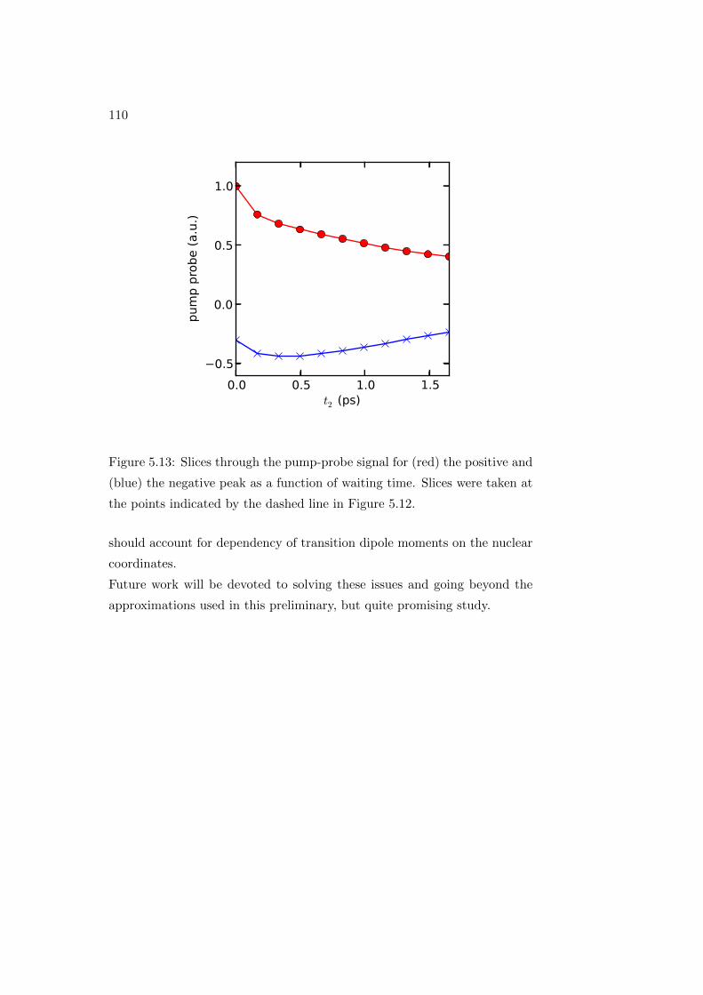
110
0.0 0.5 1.0 1.5t2 (ps)
−0.5
0.0
0.5
1.0pum
p p
robe (
a.u
.)
Figure 5.13: Slices through the pump-probe signal for (red) the positive and
(blue) the negative peak as a function of waiting time. Slices were taken at
the points indicated by the dashed line in Figure 5.12.
should account for dependency of transition dipole moments on the nuclear
coordinates.
Future work will be devoted to solving these issues and going beyond the
approximations used in this preliminary, but quite promising study.

111
Figure 5.14: Calculated two-dimensional optical spectra for various waiting
times.

112

Chapter 6
Conclusions
The present work was devoted to the study of linear and two-dimensional
electronic spectroscopy of DNA nucleobases. Introduction of the theoretical
background, explanation of the used computational methods and description
of main results are provided.
UV photochemistry of nucleic acids is a subject of big interest, as UV
electronic excitations trigger a sequence of events which may lead to UV-
induced damage of DNA, with all its profound and vast biological conse-
quences (e.g. mutagenic and carcinogic effects). This has a big impact in
understanding of exact circumstances for the beginning of life on Earth,
since much of the prebiotic chemistry probably occurred under intense UV
irradiation.
On the other side, investigating the fundamental processes underlying UV
photochemistry of DNA constituents can have extremely important medical
applications, for what concerns the damaging processes following the UV
irradiation, which is one of the main cause of skin cancer [126].
To date, not so much is known about the dynamics of the electronic states
of these DNA macromolecules.
In this work, we intend to provide for the first time a tractable low-
dimensional model of the excited state dynamics of DNA nucleobases in
presence of external fluctuations induced by the solvent. In order to do so,
we follow the so-called reductionist approach and start our analysis from
the single nucleobases and their UV photophysics, studied in terms of linear
113

114
and 2DES spectroscopy.
After UV photoexcitation, all four DNA nucleobases return to the ground
state by means of internal conversion processes at the scale of a few picosec-
onds, a fact that has been often related to the intrinsic photostability of these
bases. The electronic excited states involved in such decay processes have
been intensively investigated in the last decades, but no common picture for
the relaxation of DNA nucleobases have been reached yet.
Understanding and simulating linear absorption spectra of DNA con-
stituents is a first necessary step in this direction, and this is the motivation
for the first part of the present study, where the UV absorption spectra
of the four DNA nucleobases in aqueous solution have been modeled. The
calculation has been performed by using a combination of time-dependent
density functional theory and the semiclassical nuclear ensemble method
[56]. The water molecules forming the microsolvation shell are explicitly in-
cluded and the entire complex is placed in a bulk water solvent represented
as a continuous polarizable dielectric medium (PCM). The simulated spec-
tra are compared to experimentally measured absorption spectra. Apart
from a systematic shift of 0.3 eV of the absorption peaks, the calculated
photoabsorption spectra reproduce the measured ones with good accuracy.
The effect of the solvation shell seems significant: the lone electron pairs
in the hydrogen bonding with the solvating water molecules systematically
increases the energies of vertical excitation into the nπ∗-type states. As a
consequence, the energies of vertical excitation into the nπ∗-type states are
higher by a few tenths of an electronvolt for the microsolvated bases than
the energies for the excitation into the lowest ππ∗-states. This is in contrast
to the case of isolated nucleobases, where the energies of the lowest nπ∗-
and ππ∗-type states are comparable.
The additional inclusion of vibrational broadening, implicit in the use of the
semiclassical ensemble method, seems essential for a reliable comparison of
simulated photoabsorption spectra with experimental data, as the peaks in
the vibrationally-broadened spectra are consistently red-shifted with respect
to the vertical excitation energies calculated at the ground-state equilibrium
geometries.
115
One of the goals of this project is also to determine optical properties of
DNA nucleobases in terms of the third-order response function, which yields
a direct connection of the theoretical modelings to experimental results of
4-wave-mixing time-resolved optical spectroscopies, in particular to photon-
echo-based 2D-UV and transient absorption spectroscopies. The developed
theoretical picture was obtained in close collaboration with the experimen-
talists at the Max Planck Institute for the Structure and Dynamics of Matter
(MPSD), who provided the reference experimental data and a spectroscopic
model derived from the analysis of experimental observations. The investi-
gated system for this study was the 9H- isomer of adenine, the most studied
DNA nucleobase in the past. A minimal kinetic model was derived from
the experimental results: excitation to a bright ππ∗ state is followed by fast
population transfer to a dark nπ∗ state via a conical intersection. The deac-
tivation of the nπ∗ state population is due to a second conical intersection
connecting the dark and the ground state.
The non-Markovian quantum dynamics of such system has been simulated
by means of two methods: Time Nonlocal (TNL) [69], and Hierarchy Equa-
tions of Motion (HEOM) [77, 79] approach. 2DES and pump probe spectra
have been simulated and compared with the available experimental data,
leading in both cases to good agreement between the experiment and the-
ory.
For the HEOM approach, the linear vibronic coupling model [124] has been
used, while in the TNL treatment, no vibronic structure of the excited states
was accounted for. Therefore, the HEOM approach leads to more accurate
results, even though a good agreement for the pump-probe spectra at short
delay times was not yet reached. However, the theoretical modelings pre-
sented here fully supports the spectroscopic model derived from experiments
and the proposed route for deactivation of population in DNA nucleobases
via two conical intersections [109].
Several issues still limit the performance of both TNL and HEOM ap-
proaches, for instance, the use of the Condon approximation and the high
temperature limit. Further spectroscopic studies in terms of ultrafast 2D
spectroscopy are necessary to confirm the results of the present study, which
will serve as a basis for future simulations and experimental investigations.

116
The natural continuation of the research described in the present work
is the extension of the model from single nucleobases to nucleotides (and
nucleosides) polymers. Simulation of linear absorption, circular dichroism
and 2DES spectra for dimers, and even longer chains of nucleobases will be
the next steps of the research, with the goal of reproducing the experimental
data, available for chains of 2, 4 and 10 DNA monomers.
The modeling of such systems clearly would imply taking into account the
exciton couplings between the DNA monomers and charge transfer due to
the interaction of more monomers within a single (or double) DNA strand,
already studied and introduced in Chapter 1.
The present work is the first milestone towards the development of a working
exciton model for single-stranded, and furthermore double-stranded DNA,
so that we can gain a full understanding of the forthcoming 2D spectra.
A suitable system for a promising application of the semiclassical en-
samble method is the cyclobutane thymine dimer, the major DNA lesion
induced in human skin by sunlight, whose recognition and repair are inten-
sively studied for the implication on human health [127]. Linear absorption
and circular dichroism spectroscopies of such molecule are possible topics
for future research.
Bibliography
[1] C. E. Crespo-Hernandez, B. Cohen, P.M. Hare, B. Kohler Chem. Rev.,
2004, 104, 1977-2009.
[2] C.T. Middleton, K. de la Harpe, C. Su, Y.K. Law; C. E. Crespo-
Hernandez, B. Kohler Annu. Rev. Phys. Chem., 2009, 60, 217-239.
[3] K. Kleinermanns, D. Nachtigallova, M.S. de Vries Int. Rev. Phys.
Chem., 2013, 32, 308-342.
[4] W. C. Chung, Z. Lan, Y. Ohtsuki, N. Shimakura, W. Domcke, Y.
Fujimura Phys. Chem. Chem. Phys., 2007,9, 2075-2084.
[5] S. Matsika J. Phys. Chem. A, 2005, 109, 7538-7545.
[6] M. Barbatti, A. J. Aquino, J. J. Szymczak, D. Nachtigallova, P. Hobza,
H. Lischka PNAS, 2010, 107, 21453-21458.
[7] C. E. Crespo-Hernandez, B. Kohler J. Phys. Chem. B, 2004, 108,
11182–11188.
[8] F. Santoro, R. Improta, P. Segado, A. Lami Photochem. Photobiol. Sci.,
2013, 12(8), 1527-1543.
[9] M. Barbatti et al. Phys. Chem. Chem. Phys., 2010, 12, 4959-4967.
[10] A. Nenov, J. Segarra-Marti, A. Giussani, I. Conti, I. Rivalta, E. Du-
mont, V. K. Jaiswal, S. F. Altavilla, S. Mukamel, M. Garavelli Faraday
Discuss., 2015, 177, 345-362.
[11] S. Mai, M. Richter, P. Marquetand, L. Gonzalez Top. Curr. Chem.,
2015, 355, 99-154.
117

118
[12] S. Ulrich, T. Schultz, M. Z. Zgierski, A. Stolow Phys. Chem. Chem.
Phys., 2004, 6, 2796-2801.
[13] S. Ullrich, T. Schultz, M.Z. Zgierski, A. Stolow J. Am. Chem. Soc.,
2004, 126, 2262–2263.
[14] L. Serrano-Andres, M. Merchan, A. C. Borin Proc. Natl. Acad. Sci.
U.S.A., 2006, 103 (23), 8691-8696.
[15] E. Fabiano, W. Thiel J. Phys. Chem. A, 2008, 112(30), 6859-6863.
[16] J. R. Platt Journal of Chemical Physics, 1949, 17, 484-495.
[17] A. F. Fucaloro, L. S. Forster, J. A. Chem. Soc., 1971, 93, 6443-6448.
[18] H. Kang, K. Lee, B. Jung, Y. Ko, S. K. Kim J. Am. Chem. Soc., 2002,
124, 12958-12959.
[19] H. Kang, B. Jung, S. K. Kim J. Chem. Phys., 2003, 118, 6717–6719.
[20] C. Canuel, M. Mons, F. Piuzzi, B. Tardivel, I. Dimicoli, M. Elhanine
J. Chem. Phys., 2005, 122, 074316-1 - 074316-6.
[21] M. Barbatti, H. Lischka J. Am. Chem. Soc., 2008, 130(21), 6831–6839.
[22] Y. Lei, S. Yuan, Y. Dou, Y. Wang, Z. Wen J. Phys. Chem. A, 2008,
112(37), 8497–8504.
[23] A. L. Sobolewski, W. Domcke Eur. J. Phys. D, 2002, 20, 369-374.
[24] S. Perun, A. L. Sobolewski, W. Domcke Chem. Phys., 313, 107–112.
[25] H. R. Mahler, B. Kline and B. D. Mehrotra J. Mol. Biol., 1964, 9,
801-811.
[26] T. Takaya, C. Su, K. de La Harpe, C. E. Crespo-Hernandez, B. Kohler
Proc. Natl. Acad. Sci. USA, 2008, 105, 10285–10290.
[27] F. Plasser, A.J.A. Aquino, H. Lischka, D. Nachtigallova Top. Curr.
Chem., 2015, 356, 1–38.

119
[28] A.J.W.G. Visser, O.J. Rolinski BASIC PHOTOPHYSICS Photobio-
logical Science Online (photobiology.info).
[29] J. Von Neumann, E. P. Wigner Z. Physik, 1929, 30, 465-467.
[30] F. Hund Z. Physik, 1927, 40, 742-764.
[31] S.M.G. Faeder, D.M. Jonas Journal of Physical Chemistry A, 1999,
103(49), 10489–10505.
[32] J.D. Hybl, A.A. Ferro, D.M. Jonas Journal of Chemical Physics, 2001,
115(14), 6606–6622.
[33] M. Khalil, N. Demirdoven, A. Tokmakoff Physical Review Letters, 2003,
90, 047401/1-047401/4.
[34] Shaul Mukamel. Principles of Nonlinear Optical Spectroscopy, Oxford
University Press, 1995.
[35] W. Zhuang, T. Hayashi, and S. Mukamel Angewandte Chemie-
international Edition, 2009, 48(21), 3750–3781.
[36] M. H. Cho. Chemical Reviews, 2008, 108(4), 1331–1418.
[37] J. Allen Myers Two-Dimensional Electronic Spectroscopy of the Pho-
tosystem II D1D2-cyt.b559 Reaction Center, University of Michigan,
2010.
[38] K. Lazonder, M. S. Pshenichnikov, D. A. Wiersma Optics Letters, 2006,
31(22), 3354–3356.
[39] J. P. Ogilvie Advances In Atomic, Molecular, and Optical Physics, 2009,
57, 249–321.
[40] P. Pyykko, J. F. Stanton Chem. Rev. 2012, 112, 1-3.
[41] W. Thiel Angew. Chem. Int. Ed., 2011, 50, 9216–9217.
[42] D. I. Lyakh, M. Musial, V. F. Lotrich, R. J. Bartlett Chem. Rev., 2011,
112,182-243.
[43] D. Cremer, J. A. Pople J. A. Chem. Soc., 1975, 97, 1354–1358.
120
[44] W. Thiel New methods in computational quantum mechanics, Advances
in chemical physics., 1996, 93, 703-757.
[45] W. Thiel WIREs Comput Mol Sci, 2014, 4, 145-157.
[46] A. J. Cohen, P. Mori-Sanchez, W. Yang Chem Rev, 2012, 112, 289–320.
[47] F. Jensen, Introduction to Computational Chemistry, 2nd edition, John
Willey and Sons Ltd.: New York, 2007.
[48] K. Burke J. Chem. Phys., 2012, 136, 150901-1 - 150901-9
[49] L. H. Thomas Proc. Cambridge. Phil. Soc. 23, 542-548.
[50] P. Hohenberg, W. Kohn Phys. Rev. 1964, 136, B864-B871.
[51] W. Kohn, J. Sham Phys.Rev., 1965, 140, A1133-A1138.
[52] Runge, E.; Gross, E. K. U. Phys. Rev. Lett. 52, 997–1000, 1984.
[53] K. Burke, E. K. U. Gross A guided tour of time-dependent density func-
tional theory in Density functional: Theory and applications, Springer,
Berlin, 1998.
[54] R. van Leeuwen Phys. Rev. Lett., 1999, 82, 3863–3866.
[55] F. Plasser, R. Crespo-Otero, M. Pederzoli, J. Pittner, H. Lischka, M.
Barbatti J. Chem. Theory Comput., 2014, 10, 1395-1405.
[56] R. Crespo-Otero, M. Barbatti Theor. Chem. Acc., 2012, 131(6), 1-14.
[57] M. Barbatti, A. J. A. Aquino, H. Lischka Phys. Chem. Chem. Phys.,
2010, 12 (19), 4959-4967.
[58] V. May, O. Kuhn Charge and Energy Transfer Dynamics in Molecular
Systems, 3rd, Revised and Enlarged Edition, Wiley, 2011.
[59] M. Barbatti, G. Granucci, M. Persico, M. Ruckenbauer, M. Vazdar,
M. Eckert-Maksic, H. Lischka J. Photochem. Photobio. A, 2007, 190,
228-240.

121
[60] M. Barbatti, M. Ruckenbauer, F. Plasser, J. Pittner, G. Granucci, M,
Persico, H. Lischka WIREs: Comp. Mol. Sci., 2014, 4, 26-33.
[61] Gaussian 09, Revision E.02, M. J. Frisch, G. W. Trucks, H. B. Schlegel,
G. E. Scuseria, M. A. Robb, J. R. Cheeseman, G. Scalmani, V. Barone,
B. Mennucci, G. A. Petersson, H. Nakatsuji, M. Caricato, X. Li, H.
P. Hratchian, A. F. Izmaylov, J. Bloino, G. Zheng, J. L. Sonnenberg,
M. Hada, M. Ehara, K. Toyota, R. Fukuda, J. Hasegawa, M. Ishida,
T. Nakajima, Y. Honda, O. Kitao, H. Nakai, T. Vreven, J. A. Mont-
gomery, Jr., J. E. Peralta, F. Ogliaro, M. Bearpark, J. J. Heyd, E.
Brothers, K. N. Kudin, V. N. Staroverov, R. Kobayashi, J. Normand,
K. Raghavachari, A. Rendell, J. C. Burant, S. S. Iyengar, J. Tomasi,
M. Cossi, N. Rega, J. M. Millam, M. Klene, J. E. Knox, J. B. Cross,
V. Bakken, C. Adamo, J. Jaramillo, R. Gomperts, R. E. Stratmann,
O. Yazyev, A. J. Austin, R. Cammi, C. Pomelli, J. W. Ochterski, R. L.
Martin, K. Morokuma, V. G. Zakrzewski, G. A. Voth, P. Salvador, J.
J. Dannenberg, S. Dapprich, A. D. Daniels, O. Farkas, J. B. Foresman,
J. V. Ortiz, J. Cioslowski, and D. J. Fox, Gaussian, Inc., Wallingford
CT, 2009.
[62] A.J.A. Aquino, D. Nachtigallova, P. Hobza, D. G. Truhlar, G.C. Hattig,
H. Lischka J. Comput. Chem., 2011, 32(7), 1217–1227.
[63] Y. Zaho, D. G. Truhlar Theo. Chem. Account, 2007, 120(1), 215–241.
[64] David S. Weiss, J. Robin Cowdery and Ralph H. Young Electron Trans-
fer in Chemistry, Wiley, 2008.
[65] H-J. Briegel and B-G. Englert, Phys. Rev. A, 1993, 47, 3311-3329.
[66] U. Kleinekathofer The Journal of Chemical Physics, 2004, 121, 2505-
2514.
[67] R. Zwanzig Lectures in Theoretical Physics, 1961, Boulder, Colorado
3.30, Interscience, New York.
[68] F. Haake, Springer Tracts Mod. Phys., 1973, 66, 98-168.

122
[69] C. Meier, D. j. Tannor, The Journal of Chemical Physics, 1999, 111,
3365-3376.
[70] M. F. Gelin, D. Egorova, W. Domcke J. Chem. Phys., 2005, 123,
164112-1 - 164112-11.
[71] Y. Tanimura, R. Kubo J. Phys. Soc. Jpn., 1989, 58, 1850-1859.
[72] C. Kreisbeck, T. Kramer J. Phys. Chem. Lett., 2012, 3(19), 2828–2833.
[73] A. G. Dijkstra, Y. Tanimura New J. Phys., 2012, 14 (7), 073027-1 -
073027-11.
[74] M. Tanaka, Y. Tanimura J. Phys. Soc. Jpn., 2009, 78,
073802/1–073802/4.
[75] Y. Cheng, W. Hou, Y. Wang, Z. Li, J. Wei, and Y. Yan New J. Phys.,
2015, 17, 033009-1 - 033009-11.
[76] J. S. Jin, X. Zheng, and Y. J. Yan, J. Chem. Phys., 2008, 128, 234703-1
- 234703-15.
[77] M. Tanaka and Y. Tanimura J. Chem. Phys., 2010, 132, 214502-1 -
214502-11.
[78] A. Garg, J. N. Onuchic, and V. Ambegaokar J. Chem. Phys., 1985, 83,
4491-4503.
[79] Y. Tanimura J. Chem. Phys., 2012, 137, 22A550-1 - 22A550-9.
[80] M. Pola, M. Kochman, A. Picchiotti, V. Prokhorenko, R. J. D. Miller,
M. Thorwart ”Linear photoabsorption spectra and vertical excitation
energies of microsolvated DNA nucleobases in aqueous solution”, sub-
mitted to JCP.
[81] E. R. Bittner, J. Chem. Phys., 2006, 125, 094909-1 - 094909-12.
[82] R. P. Rastogi, Richa, A. Kumar, M. B. Tyagi and R. P. Sinha, Journal
of Nucleic Acids, 2010, Article ID 592980.

123
[83] B. Marchetti, T. N. V. Karsili, M. N. R. Ashfold and W.
Domcke Phys. Chem. Chem. Phys., 2016, Advance Article, doi:
10.1039/C6CP00165C.
[84] A. C. Rios and Y. Tor Astrobiology, 2012, 12, 884-891.
[85] A. C. Rios and Y. Tor Isr. J. Chem., 2013, 53, 469-483.
[86] Improta R., Barone V. Top Curr. Chem., 2015, 57, 355-329.
[87] A. W. Lange, M. A. Rohrdanz and J. M. Herbert J. Phys. Chem. B,
2008, 112, 6304-6308.
[88] Lan T., Lu Y., Fabiano E., Thiel W. Chem. Phys. Chem., 2011, Volume
12, Issue 10, 1989–1998.
[89] B. Heggen, Z. Lan, W. Thiel Phys. Chem. Chem. Phys, 2012, 14, 8137-
8146.
[90] D. Tuna, A. L. Sobolewski, W. Domcke J. Phys. Chem. A, 2014, 118,
22.
[91] F. Plasser, H. Lischka Photochem. Photobiol. Sci., 2013, 12, 1440-1452.
[92] T. Lu, Z. Lan, W. Thiel Top Curr. Chem., 2015, 356, 89-122.
[93] M. Barbatti J. Am. Chem. Soc., 2014, 136(29), 10246–10249.
[94] M. Barbatti, H. Lischka Phys. Chem. Chem. Phys., 2015, 53(6-
7)17(23), 15452-15459.
[95] S. Chaiwongwattana, M. Sapunar, A. Ponzi, P. Decleva, N Doslic J.
Phys. Chem. A., 2015, 119(43), 10637–10644.
[96] R. Szabla, J. Campos, J. E. Sponer, R. W. Gora, J. D. Sutherland
Chem. Sci., 2015, 6, 2035-2043.
[97] R. Improta, F. Santoro, L. Blancafort, Chem. Rev., 2016, 116, 3540 -
3593.
[98] Y. Zhao and D. G. Truhlar, Theor. Chem. Account, 2008, 120, 215-241.

124
[99] F. Plasser, R. Crespo-Otero, M. Pederzoli, J. Pittner, H. Lischka and
M. Barbatti, J. Chem. Theory Comput., 2014, 10, 1395-1405.
[100] D. M. York, M. Karplus J. Phys. Chem. A, 1999, 103, 11060-11079.
[101] G. Scalmani, M. J. Frisch J. Chem. Phys., 2010, 132, 114110-1 -
114110-15.
[102] B. Cohen, P. M. Hare, B. Kohler J. Am. Chem. Soc., 2003, 125,
13594-13601.
[103] L. J. Yu, R. Pang, S. Tao, H. T. Yang,D. Y. Wu, Z. Q. Tian J. Phys.
Chem. A, 2013, 117, 4286-4296.
[104] L. Serrano-Andres, M. Merchan, A. C. Borin JACS, 2008, 130, 2473-
2484.
[105] L. Serrano-Andres, M. Merchan, A. C. Borin Chem. Eur. J., 2006, 12,
6559-6571.
[106] P. G. Szalay, T. Watson, A. Perera, V. L. Lotrich, R. J. Bartlett J.
Phys. Chem. A, 2012, 116, 6702-6710.
[107] P. G. Szalay, T. Watson, A. Perera, V. Lotrich, G. Fogarasi, and
R. J. Bartlett, J. Phys. Chem. A, 2012, 116, 8851-8860.
[108] A. Tajti, G. Fogarasi, P.G. Szalay Chem. Phys. Chem., 2009, 10,
1603-1606.
[109] V. I. Prokhorenko, A. Picchiotti, and R.J. D. Miller New insight into
photophysics of DNA nucleobases, 2016, submitted to UP2016.
[110] M. F. Gelin, D. Egorova, W. Domcke J. Phys. Chem. Lett., 2010, 2,
114–119.
[111] D. Polli, P. Alto‘e, O. Weingart, K. M. Spilane, C. Manzoni, D. Brida,
G. Tomasello, G. Orlandi, P. Kukura, R. A. Mathies, et al. Nature,
2010, 467, 440–443.
[112] G. A. Worth, L. S. Cederbaum Annu. Rev. Phys. Chem., 2004, 55,
127-158.

125
[113] M. J. Bearpark, F. Bernardi, S. Clifford, M. Olivucci, M. A. Robb, B.
R. Smith, V. T. J. Am. Chem. Soc., 1996, 118, 169-175.
[114] L. Joubert-Doriol, I. G. Ryabinkin, A. F. Izmaylov J. Chem. Phys. ,
2013, 139, 234103-1 - 234103-10.
[115] K. Dorfman, K. Bennett, M. Kowalewski, and S. Mukamel Phys. Rev.
Lett., 2015, 115, 193003-1 - 193003-6.
[116] M. Kowalewski and S. Mukamel, J. Chem. Phys., 2015, 143, 044117-1
- 044117-9.
[117] R. Szabla, D. Tuna, R. W. Gora, J. Sponer, A. L. Sobolewski, and W.
Domcke J. Phys. Chem. Lett., 2013, 4, 2785-2788.
[118] K. Saita, M. G. Nix, and D. V. Shalashilin Phys. Chem. Chem. Phys.,
2013, 15, 16227-16235.
[119] J. Krmar, M. F. Gelin, D. Egorova, and W. Domcke J. Phys. B: At.
Mol. Opt. Phys., 2014, 47, 124019-1 - 124019-9.
[120] A. Nenov, A. Giussani, J. Segarra-Marti, V. K. Jaiswal, I. Rivalta,
G. Cerullo, S. Mukamel, and M. Garavelli, J. Chem. Phys., 2015, 142,
212443-1 - 212443-17.
[121] A. Nenov, J. Segarra-Marti, A. Giussani, I. Conti, I. Rivalta, E. Du-
mont, V. K. Jaiswal, S. Altavilla, and S. G. M. Mukamel, Faraday Disc.
, 2015, 177, 345-362.
[122] W. Domcke, D. R. Yarkony, and H. Koppel, Conical Intersections:
Theory, Computation and Experiment World Scientific, 2011.
[123] M. I. Hassan, W. C. Chung, N. Shimakura, S. Koseki, H. Kono, and
Y. Fujimura Phys. Chem. Chem. Phys., 2010, 12, 5317-5328.
[124] L. Seidner, W. Domcke Chem. Phys., 1994, 186, 27-40.
[125] A. Ishizaki and G. R. Fleming Proc. Natl. Acad. Sci. USA 2009, 106,
17255.

126
[126] U. Leiter, C. Garbe Advances in experimental medicine and biology,
Springer, New York, 2008, 624, 89–103.
[127] J. T. Reardon, A. Sancar Genes Dev, 2003, 17(20), 2539–2551.

Acknowledgements
I would like to aknowledge my supervisor, Prof. Dr. Michael Thorwart,
and my cosupervisor, Dr. Valentyn I. Prokhorenko, for their guidance dur-
ing my Phd studies.
Special thanks to Dr. Michal Kochman and Dr. Arend Dijkstra for their
constant help and support. The scientific collaboration with them was in-
credibly instructive and played a fundamental role in the realization of this
project.
127

128

Erklarung
Die hier vorgelegte Dissertation habe ich eigenstandig und ohne uner-
laubte Hilfe angefertigt. Die Dissertation wurde in der vorgelegten oder in
ahnlicher Form noch bei keiner anderen Institution eingereicht. Ich habe
bisher keine erfolglosen Promotionversuche unternommen.
Martina Pola
Hamburg, den 14.07.2016
129
Top Related