Download - Non-linear Goal Programming Using Multi-Objective Genetic ... · programming or minimax goal programming 6; 7, these methods are also not free from the dependence on the relative

Non-linear Goal Programming Using Multi-Objective Genetic Algorithms

Kalyanmoy Deb�

Kanpur Genetic Algorithms laboratory (KanGAL)Department of Mechanical EngineeringIndian Institute of Technology, Kanpur

Kanpur, PIN 208 016, IndiaE-mail: [email protected]

Technical Report No. CI-60/98October 1998

Department of Computer Science/XIUniversity of Dortmund, Germany

Abstract

Goal programming is a technique often used in engineering design activities primarily to find a com-promised solution which will simultaneously satisfy a number of design goals. In solving goal program-ming problems, classical methods reduce the multiple goal-attainment problem into a single objective ofminimizing a weighted sum of deviations from goals. Moreover, in tackling non-linear goal programmingproblems, classical methods use successive linearization techniques, which are sensitive to the chosenstarting solution. In this paper, we pose the goal programming problem as a multi-objective optimizationproblem of minimizing deviations from individual goals. This procedure eliminates the need of having ex-tra constraints needed with classical formulations and also eliminates the need of any user-defined weightfactor for each goal. The proposed technique can also solve goal programming problems having non-convex trade-off region, which are difficult to solve using classical methods. The efficacy of the proposedmethod is demonstrated by solving a number of non-linear test problems and by solving an engineeringdesign problem. The results suggest that the proposed approach is an unique, effective, and most practicaltool for solving goal programming problems.

Keywords: Goal programming, Genetic algorithms, Engineering design

1 Introduction

Developed in the year 1955, goal programming method has enjoyed innumerable applications in engineeringdesign activities1�5. Goal programming is different in concept from non-linear programming or optimizationtechniques in that the goal programming attempts to find one or more solutions which satisfy a number ofgoals to the extent possible. Instead of finding solutions which absolutely minimize or maximize objectivefunctions, the task is to find solutions that, if possible, satisfy a set of goals, otherwise, violates the goalsminimally. This makes the approach more appealing to practical designers compared to optimization methods.

The most common approach to classical goal programming techniques is to construct a non-linear pro-gramming problem (NLP) where a weighted sum of deviations from targets is minimized 6. The NLP problemalso contain a constraint for each goal, restricting the corresponding criterion function value to be within thespecified target values. A major drawback with this approach is that it requires the user to specify a set ofweight factors, signifying the relative importance of each criterion. This makes the approach subjective tothe user. Moreover, the weighted goal programming approach has difficulty in finding solutions in problemshaving non-convex feasible decision space. Although there exists other methods such as lexicographic goal

�Presently visiting Computer Science Department/LS11, University of Dortmund, Germany ([email protected])

1

programming or minimax goal programming6;7, these methods are also not free from the dependence on therelative weight factor for each criterion function.

In this paper, we suggest using a multi-objective genetic algorithm (GA) to solve the goal programmingproblem. In order to use a multi-objective GA, each goal is converted into an equivalent objective function.Unlike the weighted goal programming method, the proposed approach does not add any artificial constraintinto its formulation. Since, multi-objective GAs have been shown to find multiple Pareto-optimal solutions 8;9,the proposed approach is likely to find multiple solutions to the goal programming problem, each correspond-ing to a different setting of the weight factors. This makes the proposed approach independent from the user.Moreover, since no explicit weight factor for each criterion is used, the method is also not likely to have anydifficulty in finding solutions for problems having non-convex feasible decision space.

It is worthwhile to highlight here that the use of a multi-objective optimization technique to solve goalprogramming problems is not new8;9 and is novel. But the inefficiency of classical non-linear multi-objectiveoptimization methods has led the researchers and practitioners to only concentrate on solving linear goalprogramming problems. Although there are some attempts to use sequential linear goal programming ap-proaches, where a linear approximation of the non-linear problem is solved sequentially, the methods havenot been successful6. Multi-objective GAs are around for last five years or so and have been shown to solvevarious non-linear multi-objective optimization problems successfully 10�13. As a result of these interests,there exist now a number of multi-objective GA implementations 8;9;14�16. In this paper, we show how onesuch GA implementation can make the non-linear goal programming easier and practical to use.

In the remainder of the paper, we briefly discuss the concept of goal programming and argue why classicalgoal programming methods are not adequate tools. Thereafter, we present the working principle of one multi-objective GA implementation—non-dominated sorting GA (NSGA). The usefulness of the proposed approachis demonstrated by solving five different test problems and an engineering design problem using NSGA.

2 Goal Programming

Goal programming was first introduced in an application of a single-objective linear programming problem byCharnes, Cooper, and Ferguson1. However, goal programming gained popularity after the works of Ignizio 4,Lee17, and others. Romero6 presented a comprehensive overview and listed a plethora of engineering ap-plications where goal programming technique has been used. The main idea in goal programming is to findsolutions which attain a pre-defined target for one or more criterion function. If there exists no solution whichachieves targets in all criterion functions, the task is to find solutions which minimize deviations from tar-gets. Goal programming is different from non-linear programming problems (NLPs), where the main ideais to find solutions which optimizes one or more criteria 18;19. There is no concept of a goal in a mathemati-cal programming problem. We illustrate the concept of goal programming by considering a single-criterionproblem.

Let us consider a design criterion f(~x), which is a function of a solution vector ~x. In the context ofNLP, the objective is to find the solution vector ~x � which will minimize or maximize f(~x). Without loss ofgenerality, we consider criterion functions which is to be minimized (such as fabrication cost of an engineeringcomponent). In most design problems, there exists a number of constraints which make a certain portion(~x 2 F ) of the search space feasible. It is imperative that the optimal solution ~x � is feasible, that is, ~x� 2 F .In a goal programming, a target value t is chosen for every design criterion. One of the design goals may beto find a solution which attains a cost of t:

goal (f(~x) = t) ;~x 2 F : (1)

If the target cost t is smaller than the minimum possible cost f(~x �), naturally there exists no feasible solutionwhich will attain the above goal exactly. The objective of goal programming is then to find that solution whichwill minimize the deviation d between the achievement of goal and the aspiration target, t. The solution forthis problem is still ~x� and the overestimate is d = f(~x�) � t. Similarly, if target cost t is larger than themaximum feasible cost fmax, the solution of the goal programming problem is ~x which makes f(~x) = fmax.

2

However, if the target cost t is within [f(~x�); fmax], the solution to the goal programming problem is thatfeasible solution ~x which makes the criterion value exactly equal to t. Although this solution may not be theoptimal solution of the constrained f(~x), this solution is the outcome of the above goal program.

In the above example, we have considered a single-criterion problem. Goal programming is hardly usedfor single criterion problems. In fact, goal programming brings interesting scenarios when multiple criteria areconsidered. In the above example, an ‘equal-to’ type goal is discussed. However, there can be four differenttypes of goal criteria, as shown below7:

1. Less-than-equal-to (f(~x) � t),

2. Greater-than-equal-to (f(~x) � t),

3. Equal-to (f(~x) = t), and

4. Within a range (f(~x) 2 [tl; tu]).

In order to tackle above goals, usually two non-negative deviation variables (n and p) are introduced. Forthe less-than-equal-to type goal, the positive deviation p is subtracted from the criterion function, so thatf(~x) � p � t. Here, the deviation p quantifies the amount by which the criterion value has surpassed thetarget t. The objective of goal programming is to minimize the deviation p so as to find the solution for whichthe deviation is minimum. If f(~x) > t, the deviation p should take a non-zero positive value, otherwise itmust be zero. For the greater-than-equal-to type goal, a negative deviationn is added to the criterion function,so that f(~x) + n � t. The deviation n quantifies the amount by which the criterion function has not satisfiedthe target t. Here, the objective of goal programming is to minimize the deviation n. For f(~x) < t, thedeviation n should take a nonzero positive value, otherwise it must be zero. For the equal-to type goal, thecriterion function needs to have the target value t, thus both positive and negative deviations are used, so thatf(~x)� p+n = t. Here, the objective of goal programming is to minimize the summation (p+n), so that theobtained solution is minimally away from the target in either direction. If f(~x) > t, the deviation p shouldtake a non-zero positive value and if f(~x) < t, the deviation n should take a non-zero positive value. Forf(~x) = t, both deviations p and n must be zero. The fourth type of goal is handled by using two constraints:f(~x)� p � tl and f(~x)+ n � tu. The objective here is to minimize the summation (p+ n). All of the aboveconstraints can be replaced by a generic equality constraint:

f(~x)� p+ n = t: (2)

For a ‘less-than-equal-to’ type goal, the deviation n is a slack variable which makes the inequality constraintinto an equality constraint18. For a ‘range’ type goal, there are two such constraints, one with t l having p as theslack variable and the other with tu havingn as the slack variable. Thus, to solve a goal programming problem,each goal is converted into a at least one equality constraint, and the objective is to minimize all deviations pand n. Goal programming methods differ in the way the deviations are minimized. Here, we briefly discussthree popular methods, although there exists other goal programming approaches. In all methods, we assumethat there are M criterion functions f

j(~x), each having one of the above four types of goal.

2.1 Weighted Goal Programming

A composite objective function with deviations from each ofM criterion function is used, as described below:

MinimizeP

M

j=1(�jpj+ �

jnj);

Subject to fj(~x)� p

j+ n

j= t

j; for each goal j,

~x 2 Fnj; p

j� 0; for each goal j.

(3)

Here, the parameters �j

and �j

are weighting factors for positive and negative deviations of the j-th criterionfunction. For less-than-equal-to type goals, the parameter �

jis zero. Similarly, for greater-than-equal-to type

3

goals, the parameter �j

is zero. For range-type goals, there exists a pair of constraints for each criterionfunction. Usually, the weight factors �

jand �

jare fixed by the decision-maker, which makes the method

subjective to the user. We illustrate this matter through a simple example problem:

goal (f1 = 10x1 � 2);

goal (f2 =10+(x2�5)

2

10x1� 2);

Subject to F � (0:1 � x1 � 1; 0 � x2 � 10):

(4)

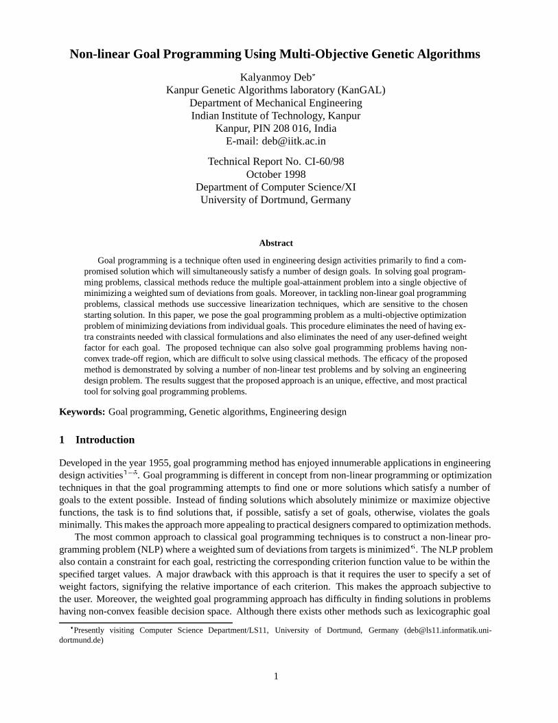
The decision space, which is the feasible solution space (~x 2 F ) is shown in Figure 1 (shaded region). The

��

��

��

��

0

2

4

6

8

10

0 0.2 0.4 0.6 0.8 1x_1

x_2 B C

Decision space

oA

Figure 1: The goal programming problem is shown insolution space.

t_2 = 2

t_1 = 2

��

��

��

��

��

f_2

A

B

C

0

4

6

8

10

0 4 6 8 10f_1

Decision space

Criterionspace Archimedian

contours

Figure 2: The goal programming problem is shown infunction space.

goal lines (f1 � 2 and f2 � 2) are also shown. It is clear that there exists no feasible solution which achievesboth goals. Figure 2 also shows that the criterion space and the decision space do not overlap. Thus, theresulting solution to above goal programming problem will violate either or both the above goals, but in aminimum sense. In solving this problem using the weighted goal programming, the following NLP problemis constructed:

Minimize �1p1 + �2p2;

Subject to 10x1 � p1 � 2;10+(x2�5)

2

10x1� p2 � 2;

0:1 � x1 � 1; 0 � x2 � 10;p1; p2 � 0:

(5)

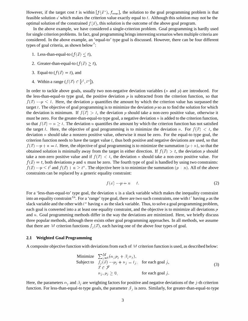
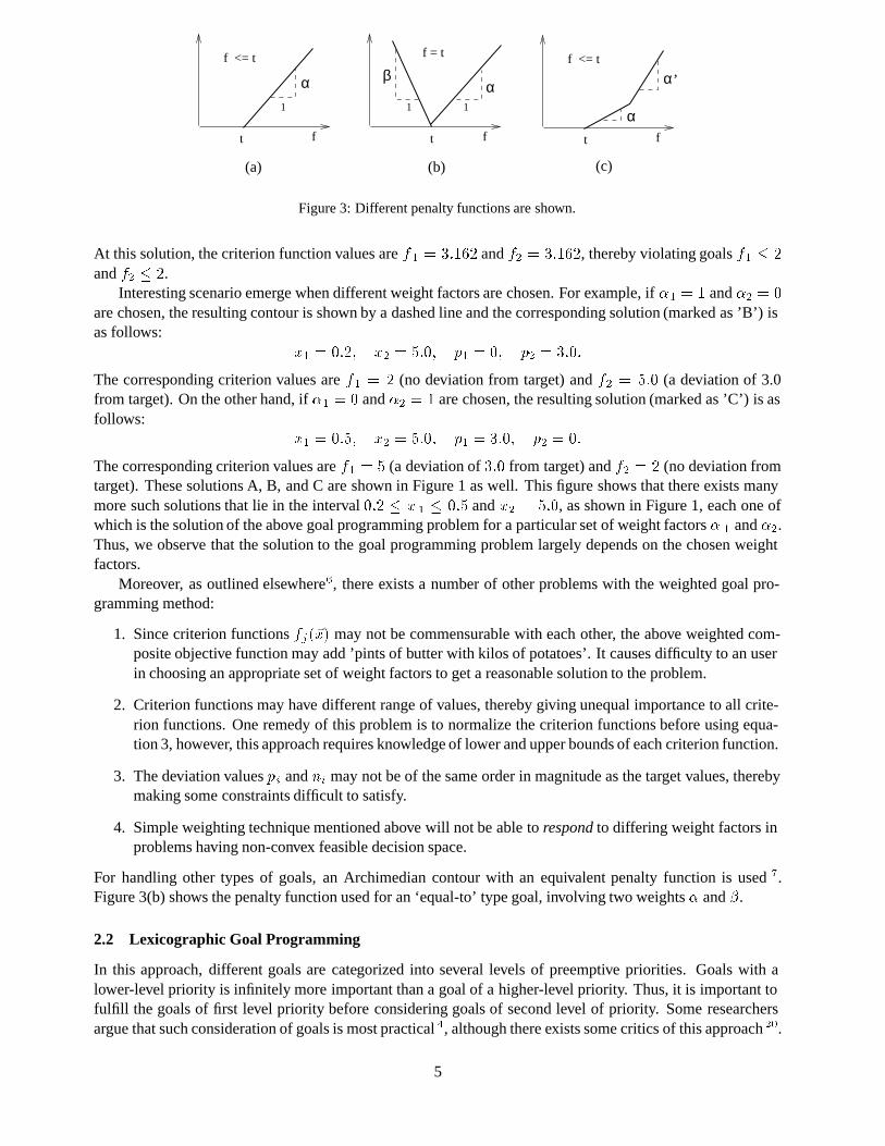
Note that in the above NLP problem the deviations n 1 and n2 in the constraints are eliminated by using a‘�’ relation. Figures 1 and 2 make the concept of goal programming clear. Since no solution in the decisionspace lies in the criterion space, the objective of goal programming is to find that solution in the decisionspace which minimizes the deviation from the criterion space in both criteria. Here comes the dependenceof the resulting solution on the weight factors � 1 and �2. By choosing a value of these weight factors, one,in fact, constructs an artificial penalty function (or known as an utility function) away from the criterionspace. The above formulation constructs a penalty function as shown in Figure 3(a) for each criterion. Thus,the objective �1p1 + �2p2 produces contours (known as Archimedian contours) as shown in Figure 2. Theconcept of the above minimization problem is to find the contour which touches the decision space. In otherwords, the minimization procedure finds that contour which has the minimum value and contains at least onesolution from the decision space. If equal importance to both objectives (that is, � 1 = �2 = 0:5) is given, theminimum contour (marked by solid lines) is shown in Figure 2 and the resulting solution (marked as ’A’) isas follows:

x1 = 0:3162; x2 = 5:0; p1 = p2 = 1:162:

4

t

f <= t

f

α1

f

α11

βf = t

t t

f <= t

f

α

α’

(a) (b) (c)

Figure 3: Different penalty functions are shown.

At this solution, the criterion function values are f 1 = 3:162 and f2 = 3:162, thereby violating goals f1 � 2and f2 � 2.

Interesting scenario emerge when different weight factors are chosen. For example, if �1 = 1 and �2 = 0are chosen, the resulting contour is shown by a dashed line and the corresponding solution (marked as ’B’) isas follows:

x1 = 0:2; x2 = 5:0; p1 = 0; p2 = 3:0:

The corresponding criterion values are f1 = 2 (no deviation from target) and f2 = 5:0 (a deviation of 3.0from target). On the other hand, if �1 = 0 and �2 = 1 are chosen, the resulting solution (marked as ’C’) is asfollows:

x1 = 0:5; x2 = 5:0; p1 = 3:0; p2 = 0:

The corresponding criterion values are f1 = 5 (a deviation of 3:0 from target) and f2 = 2 (no deviation fromtarget). These solutions A, B, and C are shown in Figure 1 as well. This figure shows that there exists manymore such solutions that lie in the interval 0:2 � x 1 � 0:5 and x2 = 5:0, as shown in Figure 1, each one ofwhich is the solution of the above goal programming problem for a particular set of weight factors � 1 and �2.Thus, we observe that the solution to the goal programming problem largely depends on the chosen weightfactors.

Moreover, as outlined elsewhere6, there exists a number of other problems with the weighted goal pro-gramming method:

1. Since criterion functions fj(~x) may not be commensurable with each other, the above weighted com-

posite objective function may add ’pints of butter with kilos of potatoes’. It causes difficulty to an userin choosing an appropriate set of weight factors to get a reasonable solution to the problem.

2. Criterion functions may have different range of values, thereby giving unequal importance to all crite-rion functions. One remedy of this problem is to normalize the criterion functions before using equa-tion 3, however, this approach requires knowledge of lower and upper bounds of each criterion function.

3. The deviation values pi

and ni

may not be of the same order in magnitude as the target values, therebymaking some constraints difficult to satisfy.

4. Simple weighting technique mentioned above will not be able to respond to differing weight factors inproblems having non-convex feasible decision space.

For handling other types of goals, an Archimedian contour with an equivalent penalty function is used 7.Figure 3(b) shows the penalty function used for an ‘equal-to’ type goal, involving two weights � and �.

2.2 Lexicographic Goal Programming

In this approach, different goals are categorized into several levels of preemptive priorities. Goals with alower-level priority is infinitely more important than a goal of a higher-level priority. Thus, it is important tofulfill the goals of first level priority before considering goals of second level of priority. Some researchersargue that such consideration of goals is most practical 4, although there exists some critics of this approach 20.

5

This approach formulates and solves a number of sequential goal programming problems. First, onlygoals and corresponding constraints of the first level priority are considered in the formulation of the goalprogramming problem and is solved. If there exists multiple solution to the problem, another goal program-ming problem is formulated with goals having the second level priority. In this case, the objective is only tominimize deviation in goals of second level priority. However, the goals of first level priority is used as hardconstraints so that obtained solution does not violate the goals of first level priority. This process continueswith goals of other higher level priorities in sequence. The process is terminated as soon as one of the goalprogramming problems results in a single solution. When this happens, all subsequent goals of higher levelpriorities are meaningless and are known as redundant goals 6. Since for solving an individual goal program-ming requires the use of the weighted goal programming approach for nonlinear problems, this method is alsonot free from the subjectiveness of users and other difficulties mentioned earlier.

2.3 Minimax Goal Programming

This approach is similar to the weighted goal programming approach, but instead of minimizing the weightedsum of deviations from targets, the maximum deviation in any goal from target is minimized. The resultingnonlinear programming problem becomes as follows:

Minimize d

Subject to �jpj+ �

jnj� d; for each goal j,

fj(~x)� p

j+ n

j= t

j; for each goal j;

~x 2 F ;nj; p

j� 0; for each goal j:

(6)

Here, the parameter d becomes the maximum deviation in any goal. Once again, this method requires thechoice of weight factors �

jand �

j, thereby making the approach subjective to user.

In the next section, we briefly discuss the multi-objective GAs. Thereafter, we show how multi-objectiveGAs can be used to solve goal programming problems which do not need any weight factor. In fact, theproposed approach simultaneously finds solutions to the same goal programming problem formed for differentweight factors, thereby making the approach both practical and different from the classical approaches.

3 Multi-Objective Genetic Algorithms

Multi-objective optimization problems give rise to a set of Pareto-optimal solutions, none of which can be saidto be better than other in all objectives. In any interesting multi-objective optimization problem, there existsa number of such solutions which are of interest to designers and practitioners. Since no one solution is betterthan any other solution in the Pareto-optimal set, it is also a goal in a multi-objective optimization to findas many such Pareto-optimal solutions as possible. Unlike most classical search and optimization problems,GAs work with a population of solutions and thus are likely (and unique) candidates for finding multiplePareto-optimal solutions simultaneously 8;9;14�16. There are two tasks that are achieved in a multi-objectiveGA:

1. Convergence to the Pareto-optimal set, and

2. Maintenance of diversity among solutions of the Pareto-optimal set.

GAs with suitable modification in their operators have worked well to solve many multi-objective optimizationproblems with respect to above two tasks. Most multi-objective GAs work with the concept of domination.In the following, we first define domination between two solutions and then describe one multi-objective GAimplementation in brief.

For a problem having more than one objective function (say, fj, j = 1; : : : ;M and M > 1), a solution

x(1) is said to weakly dominate the other solution x (2), if both the following conditions are true 7.

6

1. The solution ~x(1) is no worse (say the operator � denotes worse and � denotes better) than ~x (2) in allobjectives, or f

j(~x(1)) � f

j(~x(2)) for all j = 1; 2; : : : ;M objectives.

2. The solution ~x(1) is strictly better than ~x(2) in at least one objective, or f�j(~x(1)) � f�

j(~x(2)) for at least

one �j 2 f1; 2; : : : ;Mg.

With these conditions, it is clear that in a population of N solutions, the set of non-dominated solutions arelikely candidates to be the members of the Pareto-optimal set. It is important to mention here that if the firstcondition is satisfied with strict f

j(~x(1)) � f

j(~x(2)), then the solution ~x(1) is said to strongly dominate the

solution ~x(2). In the following, we describe one implementation of a multi-objective GA which attempts tofind the best set of non-dominated solutions in the search space.

3.1 Non-dominated Sorting GA (NSGA)

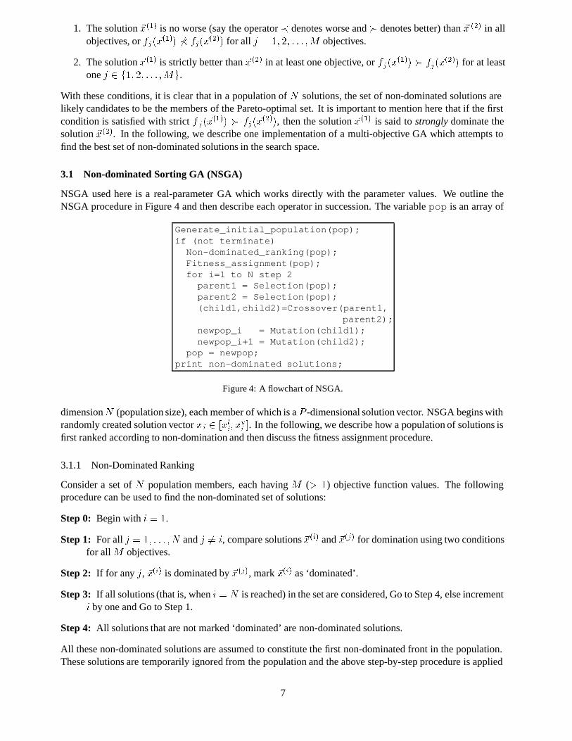
NSGA used here is a real-parameter GA which works directly with the parameter values. We outline theNSGA procedure in Figure 4 and then describe each operator in succession. The variable pop is an array of

Generate_initial_population(pop);if (not terminate)

Non-dominated_ranking(pop);Fitness_assignment(pop);for i=1 to N step 2

parent1 = Selection(pop);parent2 = Selection(pop);(child1,child2)=Crossover(parent1,

parent2);newpop_i = Mutation(child1);newpop_i+1 = Mutation(child2);

pop = newpop;print non-dominated solutions;

Figure 4: A flowchart of NSGA.

dimensionN (population size), each member of which is a P -dimensional solution vector. NSGA begins withrandomly created solution vector x

i2 [xl

i

; xui

]. In the following, we describe how a population of solutions isfirst ranked according to non-domination and then discuss the fitness assignment procedure.

3.1.1 Non-Dominated Ranking

Consider a set of N population members, each having M (> 1) objective function values. The followingprocedure can be used to find the non-dominated set of solutions:

Step 0: Begin with i = 1.

Step 1: For all j = 1; : : : ; N and j 6= i, compare solutions ~x(i) and ~x(j) for domination using two conditionsfor all M objectives.

Step 2: If for any j, ~x(i) is dominated by ~x(j), mark ~x(i) as ‘dominated’.

Step 3: If all solutions (that is, when i = N is reached) in the set are considered, Go to Step 4, else incrementi by one and Go to Step 1.

Step 4: All solutions that are not marked ‘dominated’ are non-dominated solutions.

All these non-dominated solutions are assumed to constitute the first non-dominated front in the population.These solutions are temporarily ignored from the population and the above step-by-step procedure is applied

7

again. The resulting non-dominated solutions are assumed to constitute the second non-dominated front. Thisprocedure is continued until all population members are assigned a front. Thus, a population of size N couldbe classified into a minimum of one non-dominated front of sizeN or a maximum of N non-dominated frontsof size one.

An aspect of this method is that practically any number of objectives can be used. Both minimizationand maximization problems can also be handled by this algorithm. The only place a change is required forthe above two cases is the way the non-dominated solutions are identified (according to the conditions fordominance presented earlier). The next step is to assign fitness to each solution in the population.

3.1.2 Fitness Assignment

Since all solutions in a particular non-dominated front are equally important, all are assigned the same fitnessvalue. We begin with solutions of the first non-dominated front. A large dummy fitness value (equal to N )is assigned to each non-dominated solution of the first front. However, in order to maintain diversity amongsolutions, these non-dominated solutions are then shared with their dummy fitness values. Sharing methodis discussed briefly in the next subsection. Sharing is achieved by dividing the dummy fitness value of anindividual by a quantity (called the niche count) proportional to the number of individuals around it. Thisprocedure causes multiple optimal solutions to co-exist in the population. The worst shared fitness value inthe solutions of the first non-dominated front is noted for further use.

A dummy fitness value, a little smaller than the worst shared fitness value observed in solutions of firstnon-dominated set, is assigned to all members of the second non-dominated front. Thereafter, the sharingprocedure is performed among the solutions of the second non-domination front and shared fitness values arefound as before. This process is continued till all population members are assigned a shared fitness value.

3.1.3 Sharing procedure

Given a set of nk

solutions in the k-th non-dominated front each having a dummy fitness value fk, the sharing

procedure is performed in the following way for each solution i = 1; 2; : : : ; nk:

Step 1: Compute a normalized Euclidean distance measure with another solution j in the k-th non-dominatedfront, as follows:

dij=

vuut PXp=1

x(i)p� x

(j)p

xup� xl

p

!2

;

where P is the number of variables in the problem. The parameters xu

pand xl

pare the upper and lower

bounds of variable xp.

Step 2: This distance dij

is compared with a pre-specified parameter �share and the following sharing func-tion value is computed (Deb and Goldberg, 1989):

Sh(dij) =

(1�

�dij

�share

�2; if d

ij� �share,

0; otherwise.

Step 3: Increment j. If j � nk, go to Step 1 and calculate Sh(d

ij). If j > n

k, calculate niche count for i-th

solution as follows:

mi=

nkXj=1

Sh(dij):

Step 4: Degrade the dummy fitness fk

of i-th solution in the k-th non-domination front to calculate the sharedfitness, f 0

i

, as follows:

f 0i=

fk

mi

:

8

This procedure is continued for all i = 1; 2; : : : ; nk

and a corresponding f 0

i

is found. Thereafter, the smallestvalue fmin

k

of all f 0i

in the k-th non-dominated front is found for further processing. The dummy fitness of thenext non-dominated front is assigned to be f

k+1 = fmink

� �k, where �

kis a small positive number.

The above sharing procedure requires a pre-specified parameter �share, which can be calculated as follows21:

�share �0:5Ppq; (7)

where q is the desired number of distinct Pareto-optimal solutions. Although the calculation of � share dependson this parameter q, it has been been shown elsewhere9 that the use of above equation with q � 10 works inmany test problems. Moreover, the performance of NSGAs is not very sensitive to this parameter near � share

values calculated using q � 10.

3.1.4 Selection Operator

After all solutions are assigned a fitness, selection operator is used to find above-average solution stochas-tically. A stochastic remainder proportionate selection 22 is used with the fitness values, where a solution isselected as a parent in proportion to its fitness value. With such a operator, solutions of the first non-dominatedfront have higher probability of being a parent than solutions of other fronts. This is intended to search fornon-dominated regions, which will finally lead to the Pareto-optimal front. This results in quick convergenceof the population towards non-dominated regions and sharing procedure helps to distribute it over this region.Thus, selection operator helps to emphasize better solutions in the population, but does not help to create newsolutions, a matter which is performed in the following two operators.

3.1.5 Crossover Operator

Two parent solutions ~x(1) and ~x(2) obtained from selection operator are crossed with a probability pc= 0:9.

For a crossover, the solutions are crossed variable-by-variable to create two new children solutions ~y (1) and~y(2). Depending on the relative distance between the parent parameter values, children solutions are createdby using a polynomial probability distribution 23. Each variable is crossed with a probability of 0.5 using thefollowing step-by-step procedure:

Step 1: Create a random number u between 0 and 1.

Step 2: Calculate �q

as follows:

�q=

8<:

(u�)1

�c+1 ; if u � 1�

;�1

2�u�

� 1

�c+1; otherwise;

(8)

where � = 2� ��(�c+1) and � is calculated as follows:

� = 1 +2

x(2)

i

� x(1)

i

min[(x(1)

i

� xli); (xu

i� x

(2)

i

)];

where xli

and xui

are lower and upper bounds of parameter xi. The parameter �

cis the distribution index

and can take any non-negative value. A small value of �c

allows solutions far away from parents tobe created as children solutions and a large value restricts only near-parent solutions to be created aschildren solutions. In all simulations, we use �

c= 30.

Step 3: The children solutions are then calculated as follows:

y(1)i

= 0:5h(x

(1)i

+ x(2)i

)� �qjx(2)

i

� x(1)i

ji;

y(2)

i

= 0:5h(x

(1)

i

+ x(2)

i

) + �qjx(2)

i

� x(1)

i

ji:

9

3.1.6 Mutation Operator

A polynomial probability distribution 24 is used to create a solution z(j)i

in the vicinity of a parent solution

y(j)

i

. The following procedure is used for each variable with a probability pm

:

Step 1: Create a random number u between 0 and 1.

Step 2: Calculate the parameter �q

as follows:

�q =

8>>><>>>:

�2u+ (1� 2u)(1� �)�m+1

� 1�m+1

� 1;

if u � 0:5,

1��2(1� u) + 2(u� 0:5)(1� �)�m+1

� 1�m+1 ;

otherwise,

(9)

where � = min[(y(j)

i

� yli

); (yui

� y(j)

i

)]=(yui

� yli

). The parameter �m

is the distribution index formutation and takes any non-negative value. We use �

m= 100 + t (where t is the iteration number)

here.

Step 3: Calculate the mutated child as follows:

z(j)

i

= y(j)

i

+ �q(yu

i� yl

i):

The mutation probability pm

is linearly varied from 1=P till 1:0, so that, on an average, one parameter getsmutated in the beginning and all parameters get mutated at the end of a simulation run.

4 Suggested Technique

The objective in the above multi-objective GA is to find non-dominated solutions in the search space definedby the minimality or maximality conditions of the objectives. However, the above multi-objective GA can beused to solve goal programming problems. Here, we discuss a couple of changes that are necessary for thispurpose.

4.1 Formulate Objective Functions from Goals

The goals are converted to objective functions of minimizing the deviations. The conversion procedure de-pends on the type of goals used. We present them in the following table.

Type Goal Objective function� goal (fj(~x) � tj) Minimize hfj(~x)� tji

� goal (fj(~x) � tj) Minimize htj � fj(~x)i

= goal (fj(~x) = tj) Minimize jfj(~x)� tjj

Range goal (fj(~x) 2 [tlj; tu

j]) Min. max(htl

j� fj(~x)i,

hfj(~x) � tuji)

Here the bracket operator h i returns the value of the operand if the operand is positive, otherwise returns zero.This way a goal programming problem of various kinds is formulated as a multi-objective problem. Althoughsimilar other methods have been suggested in classical goal programming texts 6;7, the advantage with theabove formulation is that (i) there is no need of any additional constraint for each goal, and (ii) since GAs donot require objective functions to be differentiable, the above objective function can be used.

Although somewhat obvious, we shall show that the NLP problem of solving the weighted goal program-ming for a fixed set of weight factors is exactly the same as solving the above reformulated problem. We shallonly consider the ‘less-than-equal-to’ type goal, however the same conclusion can be made for other types of

10

goal, as well. Consider the a goal programming problem having one goal of finding solutions in the feasiblespace F for which the criterion f(x) � t. We use equation 3 to construct the corresponding NLP problem:

Minimize p

Subject to f(~x)� p � t;

p � 0;~x 2 F :

(10)

We can rewrite both constraints involving p as d � max(0; f(~x) � t). When (f(~x) � t) is negative, theabove problem has the solution d = 0 and when (f(~x) � t) is positive, the above problem has the solutiond = f(~x)� t. This is exactly what is achieved by simply solving the problem: Minimize hf(~x)� ti.

Since we now have a way to convert a goal programming problem into an equivalent multi-objectiveproblem, we can use multi-objective GAs to solve the goal programming problem. In certain cases, theremay exist a unique solution to a goal programming problem, no matter what weight factors are chosen. Insuch cases, the equivalent multi-objective optimization problem is similar to a problem without conflictingobjectives and the resulting Pareto-optimal set contains only one solution. However, in most cases, goalprogramming problems are sensitive to the chosen weight factors and resulting solution to the problem largelydepends on specific weight factors used. The advantage of using the multi-objective reformulation is that eachPareto-optimal solution corresponding to the multi-objective problem becomes the solution of the originalgoal programming problem for a specific set of weight factors. Thus, by using multi-objective GAs, we canget multiple solutions to the goal programming problem simultaneously, which are not subjective to the user.

4.2 Using Weak Condition for Dominance

Most multi-objective search and optimization algorithms use the weak condition for dominance 6 presentedearlier. In such cases, a solution ~x(1) need not be better than ~x(2) in all objectives to dominate. In theleast, if ~x(1) is better than ~x(2) in only one objective and is equal to ~x (2) in all other objectives, then ~x(1)

dominates ~x(2). NSGA finds non-dominated solutions in a population by eliminating all dominated solutions.Thus, checking with the weak condition of dominance will allow more solutions to be qualified as dominatedsolutions than checking with the string condition of dominance. For the non-dominated solutions, the oppositeis true. Thus, using the weak condition for dominance allows more strict non-dominated solutions to beretained.

With the above formulation of objective functions from goals, it is clear that there will be many solutionsfor which the formulated objective value is zero (for example, in�-type goal all solutions having f

j�t

j� 0).

Since in goal programming these solutions are not of much interest, a weak dominance condition will notinclude these solutions in the non-dominated set.

4.3 Estimating Relative Weights

After multiple solutions are found, designers can then use higher-level decision-making approaches or com-promise programming25 to choose one particular solution. Each solution~x can be analyzed to find the relativeimportance of each criterion function as follows:

wj=

jtjj=jf

j(~x)� t

jjP

M

i=1 jtij=jfi(~x)� tij: (11)

For a ‘range’ type goal, the target tj

can be substituted by either t lj

or tuj

depending on which is closer to f(~x).Moreover, the proposed approach also does not pose any other difficulties that the weighted goal program-

ming method has. Since solutions are compared criterion-wise, there is no danger of comparing butter withpotatoes, nor there is any difficulty of scaling in criterion function values. Furthermore, we shall show in thenext section that this approach allows to find critical solutions to non-convex goal programming problems,which are difficult to find using the weighted goal programming method.

11

5 Proof-of-Principle Results

In order to show the working of the proposed approach, we first solve a number of test problems. In the nextsection, we shall apply the technique on an engineering design problem. In all test problems, we have usedNSGAs described in Section 3.1, although any other multi-objective GA implementations with the reformu-lation suggested earlier can be used.

5.1 Test Problem P1

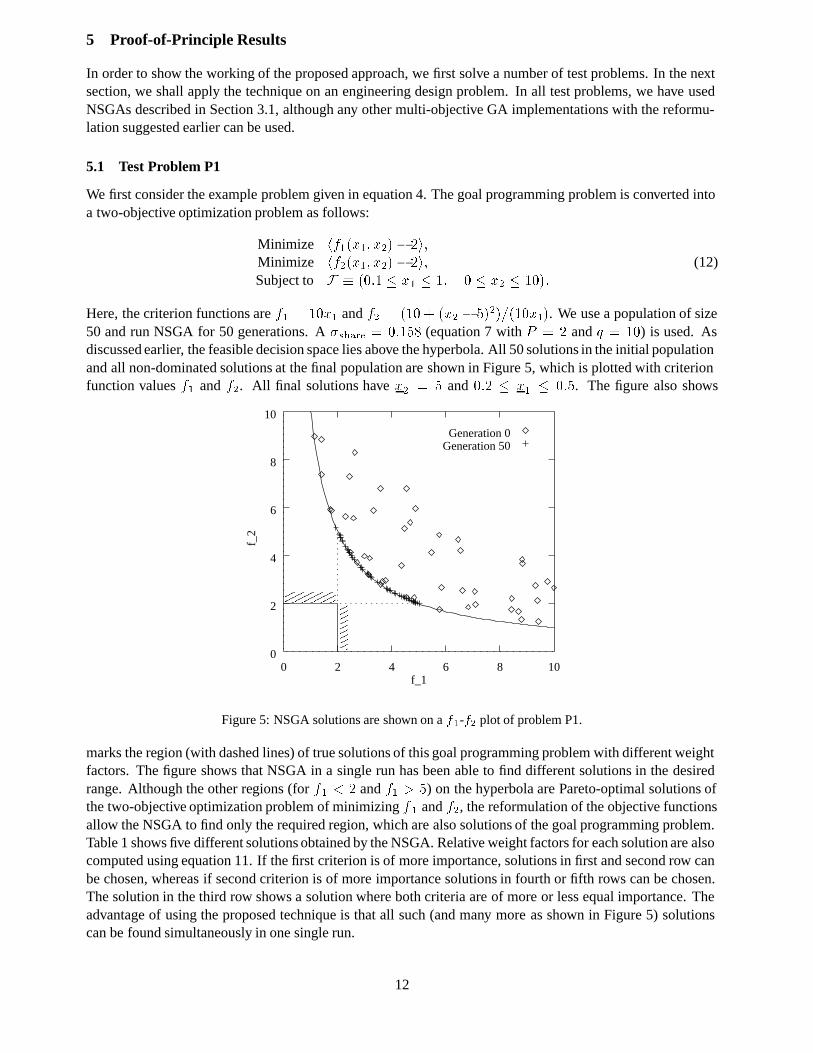
We first consider the example problem given in equation 4. The goal programming problem is converted intoa two-objective optimization problem as follows:

Minimize hf1(x1; x2)� 2i;Minimize hf2(x1; x2)� 2i;Subject to F � (0:1 � x1 � 1; 0 � x2 � 10):

(12)

Here, the criterion functions are f1 = 10x1 and f2 = (10 + (x2 � 5)2)=(10x1). We use a population of size50 and run NSGA for 50 generations. A �share = 0:158 (equation 7 with P = 2 and q = 10) is used. Asdiscussed earlier, the feasible decision space lies above the hyperbola. All 50 solutions in the initial populationand all non-dominated solutions at the final population are shown in Figure 5, which is plotted with criterionfunction values f1 and f2. All final solutions have x2 = 5 and 0:2 � x1 � 0:5. The figure also shows

0

2

4

6

8

10

0 2 4 6 8 10f_1

Generation 0Generation 50

f_2

��

��

��

��

Figure 5: NSGA solutions are shown on a f1-f2 plot of problem P1.

marks the region (with dashed lines) of true solutions of this goal programming problem with different weightfactors. The figure shows that NSGA in a single run has been able to find different solutions in the desiredrange. Although the other regions (for f1 < 2 and f1 > 5) on the hyperbola are Pareto-optimal solutions ofthe two-objective optimization problem of minimizing f 1 and f2, the reformulation of the objective functionsallow the NSGA to find only the required region, which are also solutions of the goal programming problem.Table 1 shows five different solutions obtained by the NSGA. Relative weight factors for each solution are alsocomputed using equation 11. If the first criterion is of more importance, solutions in first and second row canbe chosen, whereas if second criterion is of more importance solutions in fourth or fifth rows can be chosen.The solution in the third row shows a solution where both criteria are of more or less equal importance. Theadvantage of using the proposed technique is that all such (and many more as shown in Figure 5) solutionscan be found simultaneously in one single run.

12

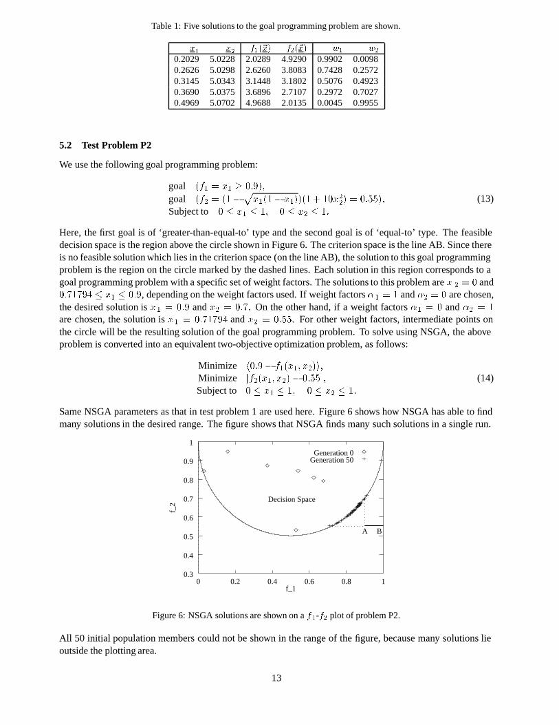
Table 1: Five solutions to the goal programming problem are shown.

x1 x2 f1(~x) f2(~x) w1 w2

0.2029 5.0228 2.0289 4.9290 0.9902 0.00980.2626 5.0298 2.6260 3.8083 0.7428 0.25720.3145 5.0343 3.1448 3.1802 0.5076 0.49230.3690 5.0375 3.6896 2.7107 0.2972 0.70270.4969 5.0702 4.9688 2.0135 0.0045 0.9955

5.2 Test Problem P2

We use the following goal programming problem:

goal (f1 = x1 � 0:9);

goal (f2 = (1�px1(1� x1))(1 + 10x22) = 0:55);

Subject to 0 � x1 � 1; 0 � x2 � 1:

(13)

Here, the first goal is of ‘greater-than-equal-to’ type and the second goal is of ‘equal-to’ type. The feasibledecision space is the region above the circle shown in Figure 6. The criterion space is the line AB. Since thereis no feasible solution which lies in the criterion space (on the line AB), the solution to this goal programmingproblem is the region on the circle marked by the dashed lines. Each solution in this region corresponds to agoal programming problem with a specific set of weight factors. The solutions to this problem are x 2 = 0 and0:71794 � x1 � 0:9, depending on the weight factors used. If weight factors � 1 = 1 and �2 = 0 are chosen,the desired solution is x1 = 0:9 and x2 = 0:7. On the other hand, if a weight factors �1 = 0 and �2 = 1are chosen, the solution is x1 = 0:71794 and x2 = 0:55. For other weight factors, intermediate points onthe circle will be the resulting solution of the goal programming problem. To solve using NSGA, the aboveproblem is converted into an equivalent two-objective optimization problem, as follows:

Minimize h0:9� f1(x1; x2)i;Minimize jf2(x1; x2)� 0:55j;Subject to 0 � x1 � 1; 0 � x2 � 1:

(14)

Same NSGA parameters as that in test problem 1 are used here. Figure 6 shows how NSGA has able to findmany solutions in the desired range. The figure shows that NSGA finds many such solutions in a single run.

Decision Space

0.3

0.4

0.5

0.6

0.7

0.8

0.9

1

0 0.2 0.4 0.6 0.8 1f_1

A B


f_2


All 50 initial population members could not be shown in the range of the figure, because many solutions lieoutside the plotting area.

13

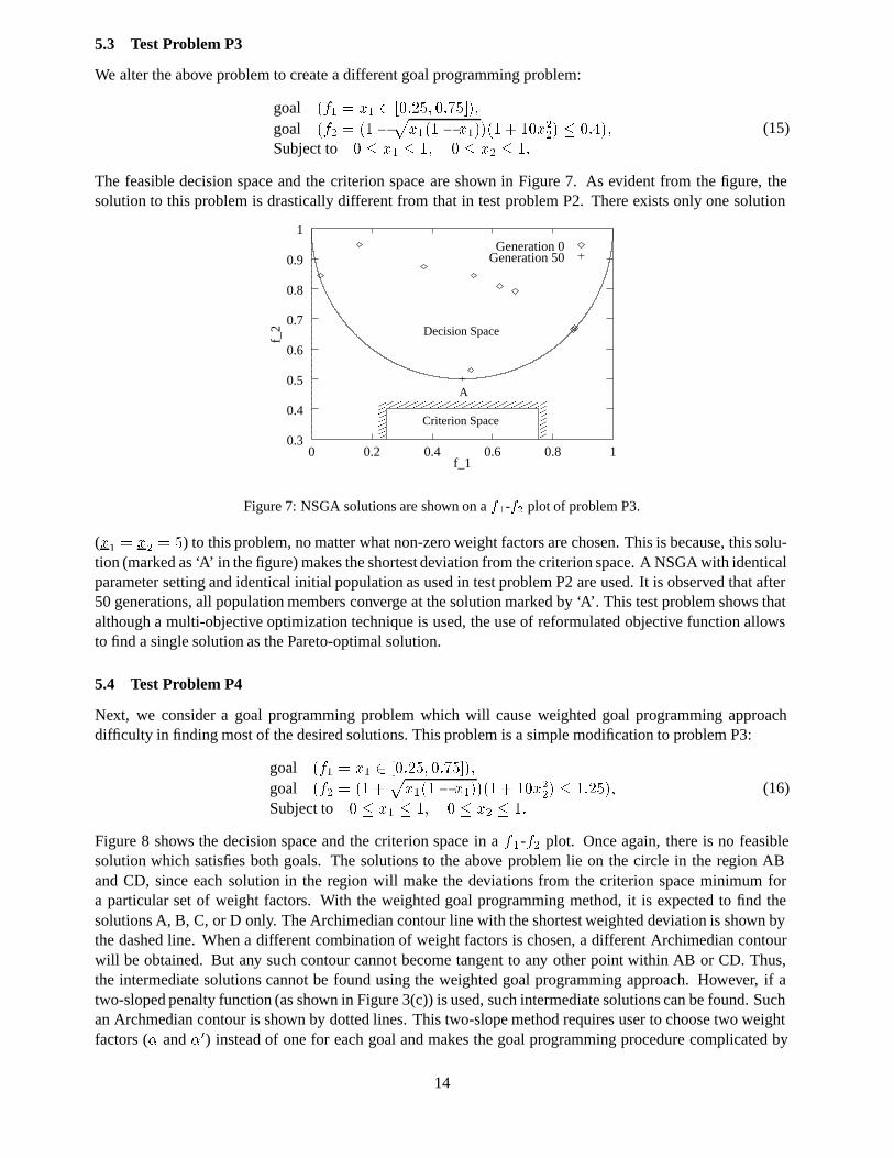
5.3 Test Problem P3

We alter the above problem to create a different goal programming problem:

goal (f1 = x1 2 [0:25; 0:75]);

goal (f2 = (1�px1(1� x1))(1 + 10x22) � 0:4);

Subject to 0 � x1 � 1; 0 � x2 � 1:

(15)

The feasible decision space and the criterion space are shown in Figure 7. As evident from the figure, thesolution to this problem is drastically different from that in test problem P2. There exists only one solution

0.3

0.4

0.5

0.6

0.7

0.8

0.9

1

0 0.2 0.4 0.6 0.8 1f_1


f_2

��

��

��

��

��

A

Decision Space

Criterion Space


(x1 = x2 = 5) to this problem, no matter what non-zero weight factors are chosen. This is because, this solu-tion (marked as ‘A’ in the figure) makes the shortest deviation from the criterion space. A NSGA with identicalparameter setting and identical initial population as used in test problem P2 are used. It is observed that after50 generations, all population members converge at the solution marked by ‘A’. This test problem shows thatalthough a multi-objective optimization technique is used, the use of reformulated objective function allowsto find a single solution as the Pareto-optimal solution.

5.4 Test Problem P4

Next, we consider a goal programming problem which will cause weighted goal programming approachdifficulty in finding most of the desired solutions. This problem is a simple modification to problem P3:

goal (f1 = x1 2 [0:25; 0:75]);

goal (f2 = (1 +px1(1� x1))(1 + 10x22) � 1:25);

Subject to 0 � x1 � 1; 0 � x2 � 1:

(16)

Figure 8 shows the decision space and the criterion space in a f 1-f2 plot. Once again, there is no feasiblesolution which satisfies both goals. The solutions to the above problem lie on the circle in the region ABand CD, since each solution in the region will make the deviations from the criterion space minimum fora particular set of weight factors. With the weighted goal programming method, it is expected to find thesolutions A, B, C, or D only. The Archimedian contour line with the shortest weighted deviation is shown bythe dashed line. When a different combination of weight factors is chosen, a different Archimedian contourwill be obtained. But any such contour cannot become tangent to any other point within AB or CD. Thus,the intermediate solutions cannot be found using the weighted goal programming approach. However, if atwo-sloped penalty function (as shown in Figure 3(c)) is used, such intermediate solutions can be found. Suchan Archmedian contour is shown by dotted lines. This two-slope method requires user to choose two weightfactors (� and �0) instead of one for each goal and makes the goal programming procedure complicated by

14

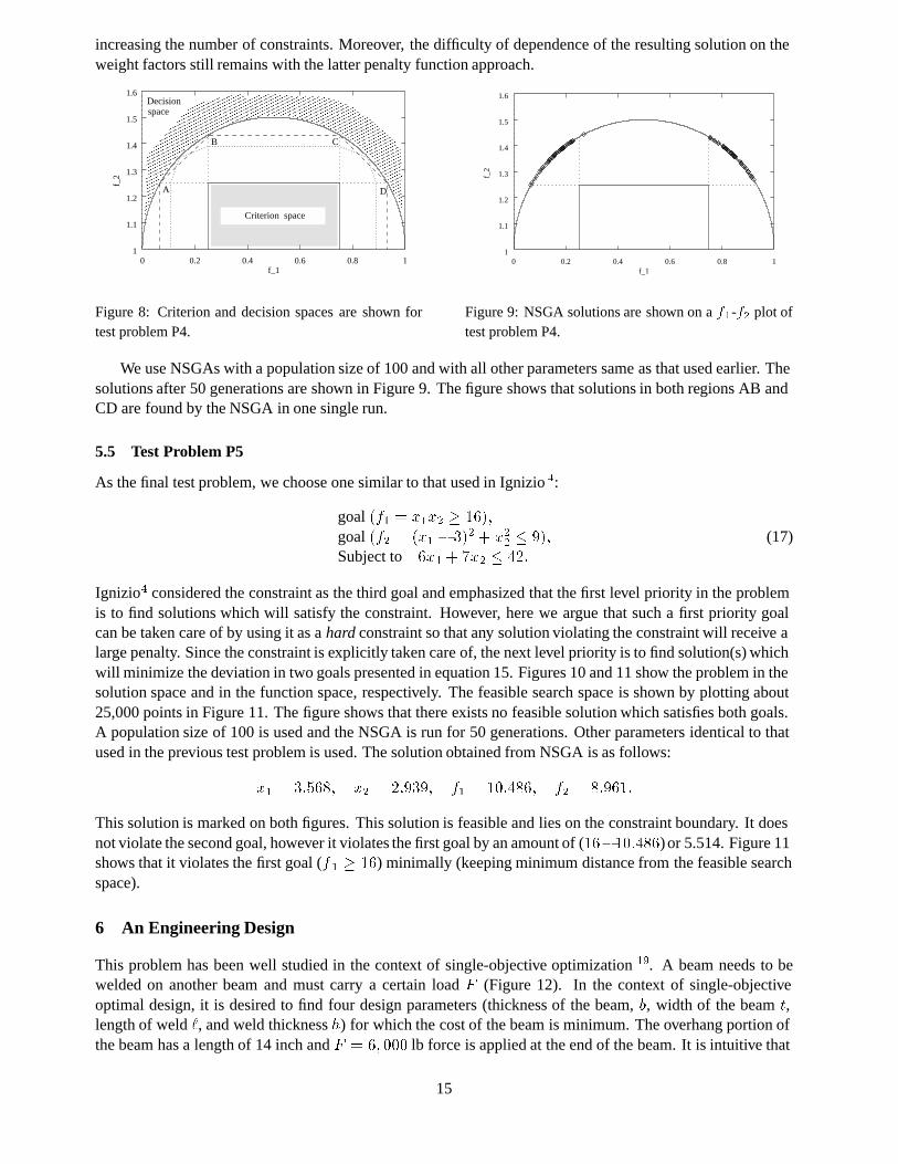
increasing the number of constraints. Moreover, the difficulty of dependence of the resulting solution on theweight factors still remains with the latter penalty function approach.

��

��

Criterion space

Decisionspace

A

B C

D

1

1.1

1.2

1.3

1.4

1.5

1.6

0 0.2 0.4 0.6 0.8 1f_1

f_2

Figure 8: Criterion and decision spaces are shown fortest problem P4.

1

1.1

1.2

1.3

1.4

1.5

1.6

0 0.2 0.4 0.6 0.8 1f_1

f_2

Figure 9: NSGA solutions are shown on a f1-f2 plot oftest problem P4.

We use NSGAs with a population size of 100 and with all other parameters same as that used earlier. Thesolutions after 50 generations are shown in Figure 9. The figure shows that solutions in both regions AB andCD are found by the NSGA in one single run.

5.5 Test Problem P5

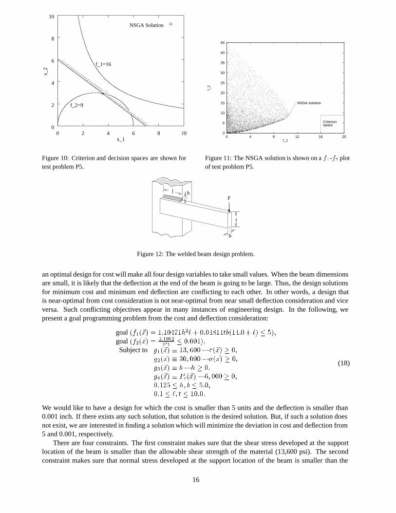
As the final test problem, we choose one similar to that used in Ignizio 4:

goal (f1 = x1x2 � 16);goal (f2 = (x1 � 3)2 + x22 � 9);Subject to 6x1 + 7x2 � 42:

(17)

Ignizio4 considered the constraint as the third goal and emphasized that the first level priority in the problemis to find solutions which will satisfy the constraint. However, here we argue that such a first priority goalcan be taken care of by using it as a hard constraint so that any solution violating the constraint will receive alarge penalty. Since the constraint is explicitly taken care of, the next level priority is to find solution(s) whichwill minimize the deviation in two goals presented in equation 15. Figures 10 and 11 show the problem in thesolution space and in the function space, respectively. The feasible search space is shown by plotting about25,000 points in Figure 11. The figure shows that there exists no feasible solution which satisfies both goals.A population size of 100 is used and the NSGA is run for 50 generations. Other parameters identical to thatused in the previous test problem is used. The solution obtained from NSGA is as follows:

x1 = 3:568; x2 = 2:939; f1 = 10:486; f2 = 8:961:

This solution is marked on both figures. This solution is feasible and lies on the constraint boundary. It doesnot violate the second goal, however it violates the first goal by an amount of (16�10:486) or 5.514. Figure 11shows that it violates the first goal (f 1 � 16) minimally (keeping minimum distance from the feasible searchspace).

6 An Engineering Design

This problem has been well studied in the context of single-objective optimization 19. A beam needs to bewelded on another beam and must carry a certain load F (Figure 12). In the context of single-objectiveoptimal design, it is desired to find four design parameters (thickness of the beam, b, width of the beam t,length of weld `, and weld thickness h) for which the cost of the beam is minimum. The overhang portion ofthe beam has a length of 14 inch and F = 6; 000 lb force is applied at the end of the beam. It is intuitive that

15

0

2

4

6

8

10

0 2 4 6 8 10x_1

f_2=9

f_1=16

NSGA Solution

x_2

��

��

Figure 10: Criterion and decision spaces are shown fortest problem P5.

0

5

10

15

20

25

30

35

40

45

0 4 8 12 16 20

f_2

f_1

NSGA solution

Criterionspace

Figure 11: The NSGA solution is shown on a f1-f2 plotof test problem P5.

b

t

hlF

Figure 12: The welded beam design problem.

an optimal design for cost will make all four design variables to take small values. When the beam dimensionsare small, it is likely that the deflection at the end of the beam is going to be large. Thus, the design solutionsfor minimum cost and minimum end deflection are conflicting to each other. In other words, a design thatis near-optimal from cost consideration is not near-optimal from near small deflection consideration and viceversa. Such conflicting objectives appear in many instances of engineering design. In the following, wepresent a goal programming problem from the cost and deflection consideration:

goal (f1(~x) = 1:10471h2`+ 0:04811tb(14:0+ `) � 5);goal (f2(~x) = 2:1952

t3b

� 0:001);Subject to g1(~x) � 13; 600� �(~x) � 0;

g2(~x) � 30; 000� �(~x) � 0;g3(~x) � b� h � 0;g4(~x) � P

c(~x)� 6; 000 � 0;

0:125 � h; b � 5:0;0:1 � `; t � 10:0:

(18)

We would like to have a design for which the cost is smaller than 5 units and the deflection is smaller than0.001 inch. If there exists any such solution, that solution is the desired solution. But, if such a solution doesnot exist, we are interested in finding a solution which will minimize the deviation in cost and deflection from5 and 0.001, respectively.

There are four constraints. The first constraint makes sure that the shear stress developed at the supportlocation of the beam is smaller than the allowable shear strength of the material (13,600 psi). The secondconstraint makes sure that normal stress developed at the support location of the beam is smaller than the

16

allowable yield strength of the material (30,000 psi). The third constraint makes sure that thickness of thebeam is not smaller than the weld thickness from a practical standpoint. The fourth constraint makes sure thatthe allowable buckling load (along t direction) of the beam is more than the applied load F . A violation ofany of the above four constraints will make the design unacceptable. Thus, in terms of discussion in Ignizio 4,satisfaction of these constraints is the first priority. The stress and buckling terms are given as follows 19:

�(~x) =

q� 02 + � 002 + `� 0� 00=

p0:25(`2+ (h+ t)2);

� 0 =6; 000p2h`

;

� 00 =6; 000(14+ 0:5`)

p0:25(`2+ (h+ t)2)

2 f0:707h`(`2=12 + 0:25(h+ t)2)g ;

�(~x) =504; 000

t2b;

Pc(~x) = 64; 746:022(1� 0:0282346t)tb3:

We handle these constraints using the bracket-operator penalty function 18. Penalty parameters of 100 and0.1 are used for the first and second criterion functions, respectively. Such dependence of penalty parameterson objective functions can be avoided by using a more efficient constraint handling technique suggestedrecently26.

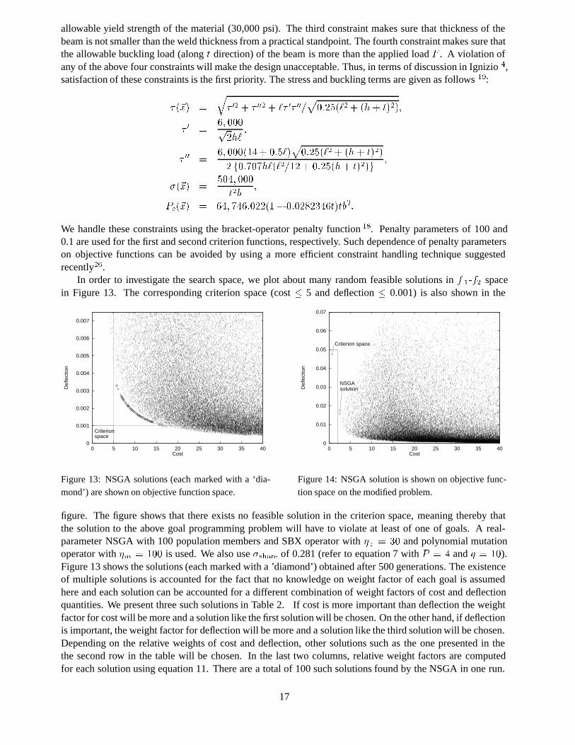
In order to investigate the search space, we plot about many random feasible solutions in f 1-f2 spacein Figure 13. The corresponding criterion space (cost � 5 and deflection � 0.001) is also shown in the

0

0.001

0.002

0.003

0.004

0.005

0.006

0.007

0 5 10 15 20 25 30 35 40

Def

lect

ion

Cost

Criterionspace

Figure 13: NSGA solutions (each marked with a ‘dia-mond’) are shown on objective function space.

0

0.01

0.02

0.03

0.04

0.05

0.06

0.07

0 5 10 15 20 25 30 35 40

Def

lect

ion

Cost

Criterion space

NSGAsolution

Figure 14: NSGA solution is shown on objective func-tion space on the modified problem.

figure. The figure shows that there exists no feasible solution in the criterion space, meaning thereby thatthe solution to the above goal programming problem will have to violate at least of one of goals. A real-parameter NSGA with 100 population members and SBX operator with �

c= 30 and polynomial mutation

operator with �m

= 100 is used. We also use �share of 0.281 (refer to equation 7 with P = 4 and q = 10).Figure 13 shows the solutions (each marked with a ’diamond’) obtained after 500 generations. The existenceof multiple solutions is accounted for the fact that no knowledge on weight factor of each goal is assumedhere and each solution can be accounted for a different combination of weight factors of cost and deflectionquantities. We present three such solutions in Table 2. If cost is more important than deflection the weightfactor for cost will be more and a solution like the first solution will be chosen. On the other hand, if deflectionis important, the weight factor for deflection will be more and a solution like the third solution will be chosen.Depending on the relative weights of cost and deflection, other solutions such as the one presented in thethe second row in the table will be chosen. In the last two columns, relative weight factors are computedfor each solution using equation 11. There are a total of 100 such solutions found by the NSGA in one run.

17

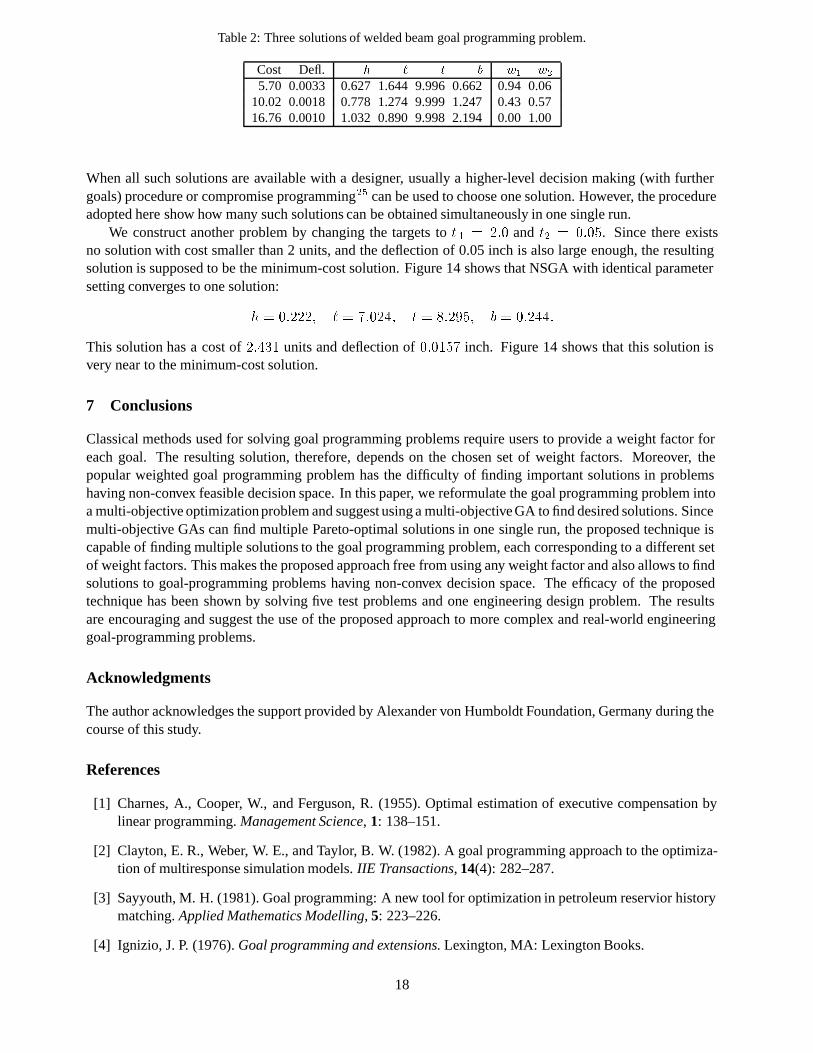
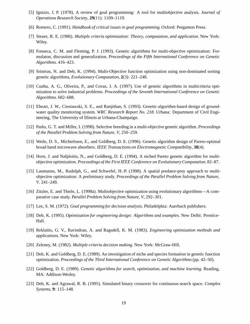
Table 2: Three solutions of welded beam goal programming problem.

Cost Defl. h ` t b w1 w2

5.70 0.0033 0.627 1.644 9.996 0.662 0.94 0.0610.02 0.0018 0.778 1.274 9.999 1.247 0.43 0.5716.76 0.0010 1.032 0.890 9.998 2.194 0.00 1.00

When all such solutions are available with a designer, usually a higher-level decision making (with furthergoals) procedure or compromise programming25 can be used to choose one solution. However, the procedureadopted here show how many such solutions can be obtained simultaneously in one single run.

We construct another problem by changing the targets to t 1 = 2:0 and t2 = 0:05. Since there existsno solution with cost smaller than 2 units, and the deflection of 0.05 inch is also large enough, the resultingsolution is supposed to be the minimum-cost solution. Figure 14 shows that NSGA with identical parametersetting converges to one solution:

h = 0:222; ` = 7:024; t = 8:295; b = 0:244:

This solution has a cost of 2:431 units and deflection of 0:0157 inch. Figure 14 shows that this solution isvery near to the minimum-cost solution.

7 Conclusions

Classical methods used for solving goal programming problems require users to provide a weight factor foreach goal. The resulting solution, therefore, depends on the chosen set of weight factors. Moreover, thepopular weighted goal programming problem has the difficulty of finding important solutions in problemshaving non-convex feasible decision space. In this paper, we reformulate the goal programming problem intoa multi-objective optimization problem and suggest using a multi-objective GA to find desired solutions. Sincemulti-objective GAs can find multiple Pareto-optimal solutions in one single run, the proposed technique iscapable of finding multiple solutions to the goal programming problem, each corresponding to a different setof weight factors. This makes the proposed approach free from using any weight factor and also allows to findsolutions to goal-programming problems having non-convex decision space. The efficacy of the proposedtechnique has been shown by solving five test problems and one engineering design problem. The resultsare encouraging and suggest the use of the proposed approach to more complex and real-world engineeringgoal-programming problems.

Acknowledgments

The author acknowledges the support provided by Alexander von Humboldt Foundation, Germany during thecourse of this study.

References

[1] Charnes, A., Cooper, W., and Ferguson, R. (1955). Optimal estimation of executive compensation bylinear programming. Management Science, 1: 138–151.

[2] Clayton, E. R., Weber, W. E., and Taylor, B. W. (1982). A goal programming approach to the optimiza-tion of multiresponse simulation models. IIE Transactions, 14(4): 282–287.

[3] Sayyouth, M. H. (1981). Goal programming: A new tool for optimization in petroleum reservior historymatching. Applied Mathematics Modelling, 5: 223–226.

[4] Ignizio, J. P. (1976). Goal programming and extensions. Lexington, MA: Lexington Books.

18

[5] Ignizio, J. P. (1978). A review of goal programming: A tool for multiobjective analysis. Journal ofOperations Research Society, 29(11): 1109–1119.

[6] Romero, C. (1991). Handbook of critical issues in goal programming. Oxford: Pergamon Press.

[7] Steuer, R. E. (1986). Multiple criteria optimization: Theory, computation, and application. New York:Wiley.

[8] Fonseca, C. M. and Fleming, P. J. (1993). Genetic algorithms for multi-objective optimization: For-mulaton, discussion and generalization. Proceedings of the Fifth International Conference on GeneticAlgorithms. 416–423.

[9] Srinivas, N. and Deb, K. (1994). Multi-Objective function optimization using non-dominated sortinggenetic algorithms, Evolutionary Computation, 2(3): 221–248.

[10] Cunha, A. G., Oliveira, P., and Covas, J. A. (1997). Use of genetic algorithms in multicriteria opti-mization to solve industrial problems. Proceedings of the Seventh International Conference on GeneticAlgorithms. 682–688.

[11] Eheart, J. W., Cieniawski, S. E., and Ranjithan, S. (1993). Genetic-algorithm-based design of ground-water quality monitoring system. WRC Research Report No. 218. Urbana: Department of Civil Engi-neering, The University of Illinois at Urbana-Champaign.

[12] Parks, G. T. and Miller, I. (1998). Selective breeding in a multi-objective genetic algorithm. Proceedingsof the Parallel Problem Solving from Nature, V, 250–259.

[13] Weile, D. S., Michielssen, E., and Goldberg, D. E. (1996). Genetic algorithm design of Pareto-optimalbroad band microwave absorbers. IEEE Transactions on Electromagnetic Compatibility, 38(4).

[14] Horn, J. and Nafploitis, N., and Goldberg, D. E. (1994). A niched Pareto genetic algorithm for multi-objective optimization. Proceedings of the First IEEE Conference on Evolutionary Computation. 82–87.

[15] Laumanns, M., Rudolph, G., and Schwefel, H.-P. (1998). A spatial predator-prey approach to multi-objective optimization: A preliminary study. Proceedings of the Parallel Problem Solving from Nature,V. 241–249.

[16] Zitzler, E. and Thiele, L. (1998a). Multiobjective optimization using evolutionary algorithms—A com-parative case study. Parallel Problem Solving from Nature, V, 292–301.

[17] Lee, S. M. (1972). Goal programming for decision analysis. Philadelphia: Auerbach publishers.

[18] Deb, K. (1995). Optimization for engineering design: Algorithms and examples. New Delhi: Prentice-Hall.

[19] Reklaitis, G. V., Ravindran, A. and Ragsdell, K. M. (1983). Engineering optimization methods andapplications. New York: Wiley.

[20] Zeleney, M. (1982). Multiple criteria decision making. New York: McGraw-Hill.

[21] Deb, K. and Goldberg, D. E. (1989). An investigation of niche and species formation in genetic functionoptimization. Proceedings of the Third International Conference on Genetic Algorithms (pp. 42–50).

[22] Goldberg, D. E. (1989). Genetic algorithms for search, optimization, and machine learning. Reading,MA: Addison-Wesley.

[23] Deb, K. and Agrawal, R. B. (1995). Simulated binary crossover for continuous search space. ComplexSystems, 9: 115–148.

19

[24] Deb, K. and Goyal, M. (1997). A robust optimization procedure for mechanical component design basedon genetic adaptive search. ASME Journal of Mechanical Design.

[25] Zeleney, M. (1973). Compromise programming. In J. L. Cochrane and M. Zeleney (Eds.) Multiple cri-teria decision making, (pp. 262–301).

[26] Deb, K. (in press). An efficient constraint handling method for genetic algorithms. Computer Methodsin Applied Mechanics and Engineering.

20