


Languages
Pages
Legal

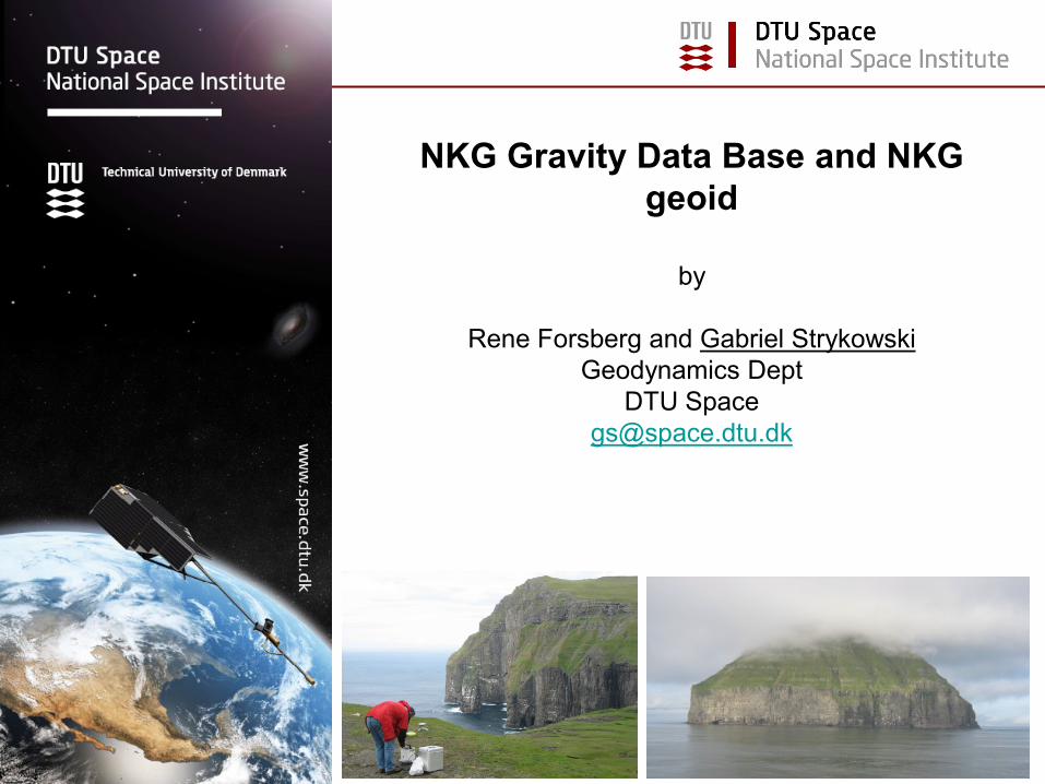
NKG Gravity Data Base and NKG
geoid
by
Rene Forsberg and Gabriel Strykowski
Geodynamics Dept
DTU Space
CONTENTS
• NKG gravity data base
• NKG geoid
History: NKG gravity data base and NKG geoid computations
NKG DB started in 1970s at Geodætisk Institut (GI), DK by prof. C.C. Tscherning,
University of Copenhagen
1980s Dag Solheim, Statens Kartverk (SK), N visited GI and wrote the present
software. Nowdays Sweden also have a copy of the DB (Läntmateriet, LM).
For many years there were two mirror sites, one in Norway (SK) and one
in Denmark (GI/KMS/DNSC/DTU Space)
Traditionally, the NKG geoid is computed in Copenhagen using the data from
NKG DB.
Over the years most countries in the area contributed to the DB. The data owner
can choose their data to be only released by permission.
The existence of the NKG gravity DB makes it straight forward to do the geoid
computations without a need to coordinate the data collection first.
Examples of NKG geoid models: NKG96, NKG2004 ... etc
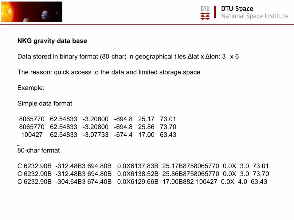
NKG gravity data base
Data stored in binary format (80-char) in geographical tiles Δlat x Δlon: 3 x 6
The reason: quick access to the data and limited storage space
Example:
Simple data format
8065770 62.54833 -3.20800 -694.8 25.17 73.01
8065770 62.54833 -3.20800 -694.8 25.86 73.70
100427 62.54833 -3.07733 -674.4 17.00 63.43
80-char format
C 6232.90B -312.48B3 694.80B 0.0X6137.83B 25.17B8758065770 0.0X 3.0 73.01
C 6232.90B -312.48B3 694.80B 0.0X6138.52B 25.86B8758065770 0.0X 3.0 73.70
C 6232.90B -304.64B3 674.40B 0.0X6129.66B 17.00B882 100427 0.0X 4.0 63.43
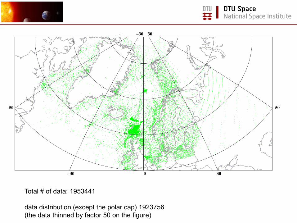
Total # of data: 1953441
data distribution (except the polar cap) 1923756
(the data thinned by factor 50 on the figure)
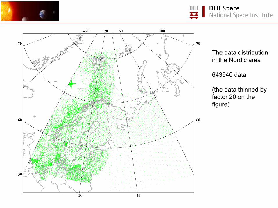
The data distribution
in the Nordic area
643940 data
(the data thinned by
factor 20 on the
figure)
Some problems with the data in the DB:
• The DB data are organized by source code. The ”vintage” (epoch) is
sometimes unknown.
• The history of correction done to the data is sometimes unknown
(e.g. The Potsdam correction, the Gulf of Riga data)
•The national height systems
This could be investigated using an A10/CG5 or an aerogravity survey (GOCINA/OCTAS)
Proposal for the issues related to the NKG gravity DB to be discussed here:
1. A systematic procedure for the quality check of the data.
2. A graphic display of the data.
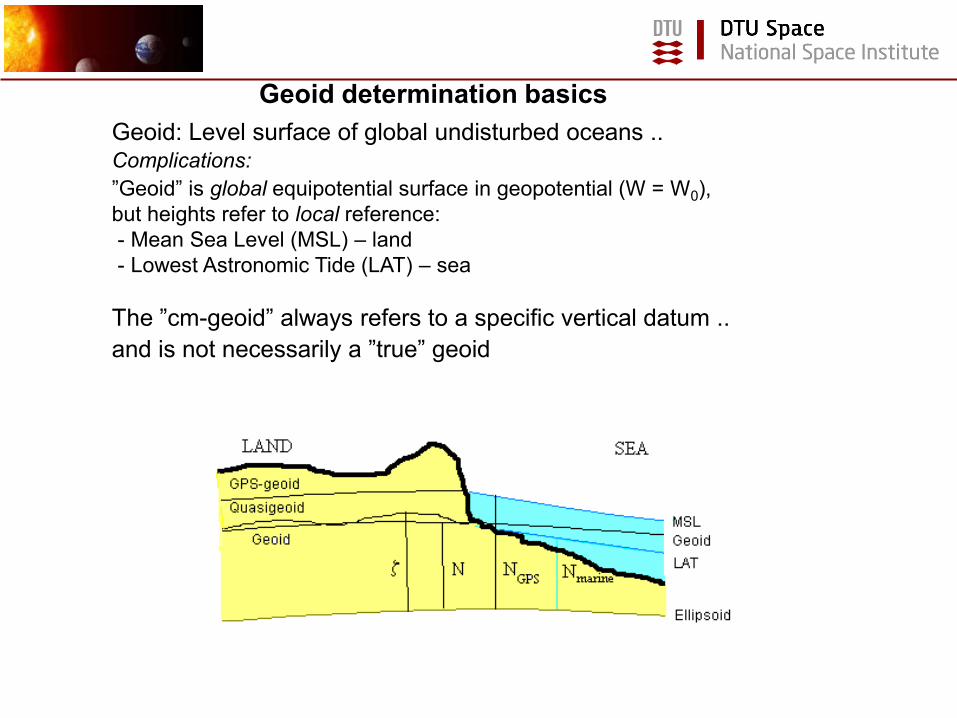
Geoid determination basics
Geoid: Level surface of global undisturbed oceans ..Complications:
”Geoid” is global equipotential surface in geopotential (W = W0),
but heights refer to local reference:
- Mean Sea Level (MSL) – land
- Lowest Astronomic Tide (LAT) – sea
The ”cm-geoid” always refers to a specific vertical datum ..
and is not necessarily a ”true” geoid
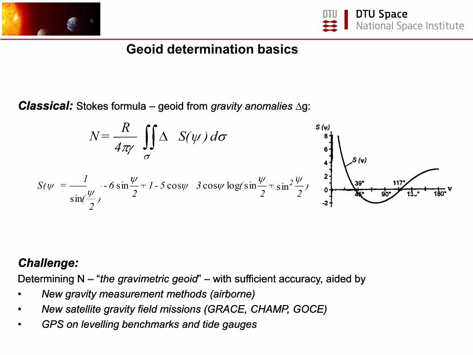
Geoid determination basics
Classical:Classical: Stokes formula Stokes formula –– geoid from geoid from gravity anomaliesgravity anomalies g:g:
Challenge:Challenge:
Determining N Determining N –– ““the gravimetric geoidthe gravimetric geoid” ” –– with sufficient accuracy, aided bywith sufficient accuracy, aided by
•• New gravity measurement methods (airborne) New gravity measurement methods (airborne)
•• New satellite gravity field missions (GRACE, CHAMP, GOCE)New satellite gravity field missions (GRACE, CHAMP, GOCE)
•• GPS on levelling benchmarks and tide gaugesGPS on levelling benchmarks and tide gauges
d ) S(g 4
R = N
)2
+2
( 3 - 5 - 1 + 2
6 -
)2
(
1 = )S( 2
sinsinlogcoscossin
sin
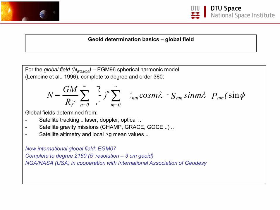
For the global field (NEGM96) – EGM96 spherical harmonic model
(Lemoine et al., 1996), complete to degree and order 360:
Global fields determined from:
- Satellite tracking .. laser, doppler, optical ..
- Satellite gravity missions (CHAMP, GRACE, GOCE ..) ..
- Satellite altimetry and local g mean values ..
New international global field: EGM07
Complete to degree 2160 (5’ resolution – 3 cm geoid)
NGA/NASA (USA) in cooperation with International Association of Geodesy
)(P)sinmS+cosmC()r
R(
R
GM = N nmnmnm
n
=0m
nN
=0n
sin
Geoid determination basics – global field
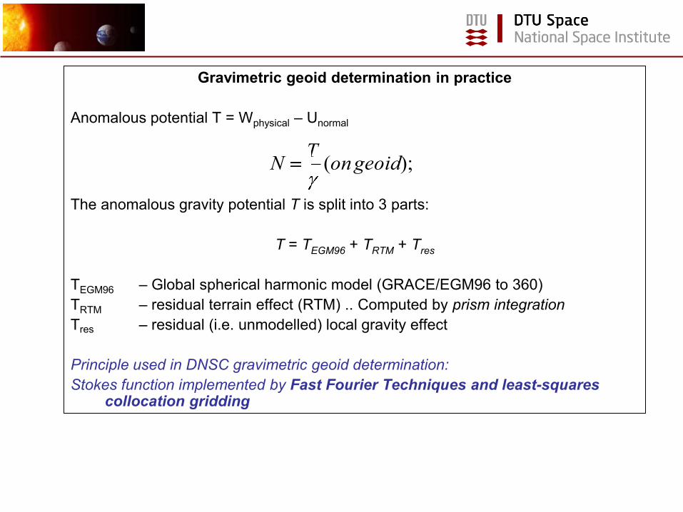
Gravimetric geoid determination in practice
Anomalous potential T = Wphysical – Unormal
The anomalous gravity potential T is split into 3 parts:
T = TEGM96 + TRTM + Tres
TEGM96 – Global spherical harmonic model (GRACE/EGM96 to 360)
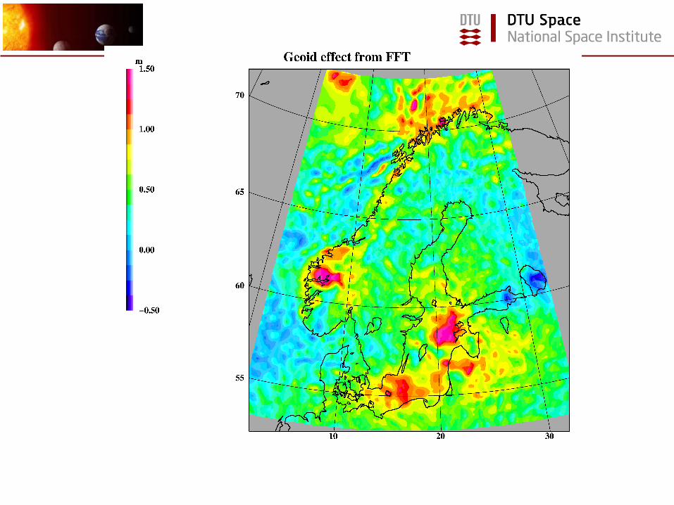
TRTM – residual terrain effect (RTM) .. Computed by prism integration
Tres – residual (i.e. unmodelled) local gravity effect
Principle used in DNSC gravimetric geoid determination:
Stokes function implemented by Fast Fourier Techniques and least-squares collocation gridding
);( geoidonT
N
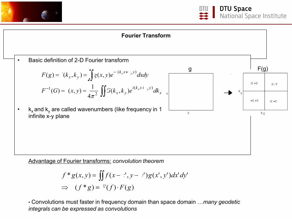
Fourier Transform
• Basic definition of 2-D Fourier transform
• kx and ky are called wavenumbers (like frequency in 1-D time domain) … defined on
infinite x-y plane
yx
ykxki
yx
ykxki
yx
dkdkekkGyxgGF
dxdyeyxgkkFgF
yx
yx
)(
2
1
)(
),(4
1),()(
),(),()(
Advantage of Fourier transforms: convolution theorem
• Convolutions must faster in frequency domain than space domain …many geodetic
integrals can be expressed as convolutions
)()()*(
'')','()','(),(*
gFfFgfF
dydxyxgyyxxfyxgf
g F(g)
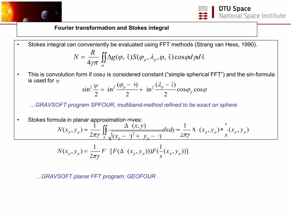
Fourier transformation and Stokes integral
• Stokes integral can conveniently be evaluated using FFT methods (Strang van Hess, 1990).
• This is convolution form if cos is considered constant (”simple spherical FFT”) and the sin-formula is used for
…GRAVSOFT program SPFOUR, multiband-method refined to be exact on sphere
• Stokes formula in planar approximation gives:
ddSgR
N pp cos),,,(),(4
))],(1())),(([
2
1),(
),(1
),(2
1
)()(
),(
2
1),(
1
2
pppppp
pppp
A pp
pp
yxs
FyxgFFyxN
yxs
yxgdxdyyyxx
yxgyxN
…GRAVSOFT planar FFT program: GEOFOUR
coscos2
)(sin
2
)(sin
2sin 222
p
pp
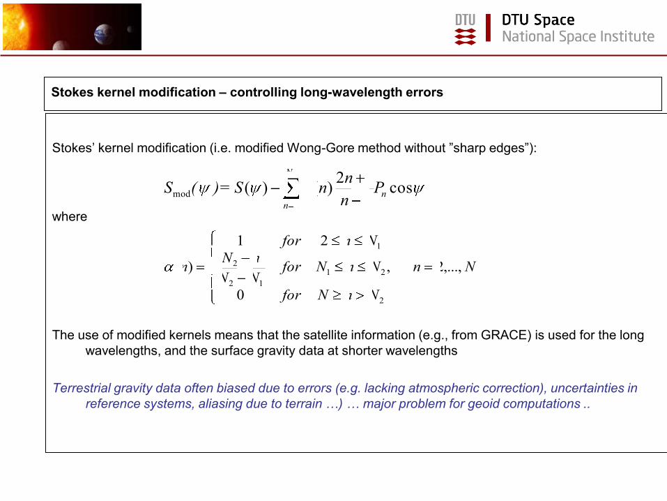
Stokes’ kernel modification (i.e. modified Wong-Gore method without ”sharp edges”):
where
The use of modified kernels means that the satellite information (e.g., from GRACE) is used for the long
wavelengths, and the surface gravity data at shorter wavelengths
Terrestrial gravity data often biased due to errors (e.g. lacking atmospheric correction), uncertainties in
reference systems, aliasing due to terrain …) … major problem for geoid computations ..
Nn
NnNfor
NnNforNN
nN
Nnfor
n ,...,2,
0
21
)(
2
21
12
2
1
cos1
12)()(
2
2
mod n
N
n
Pn
nn S= )(S
Stokes kernel modification – controlling long-wavelength errors
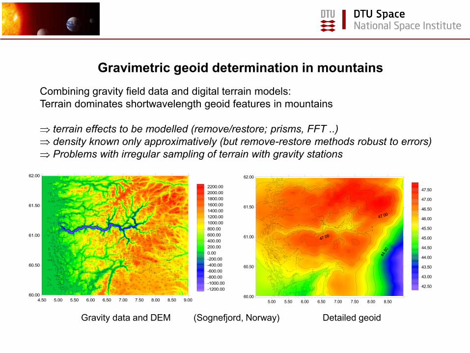
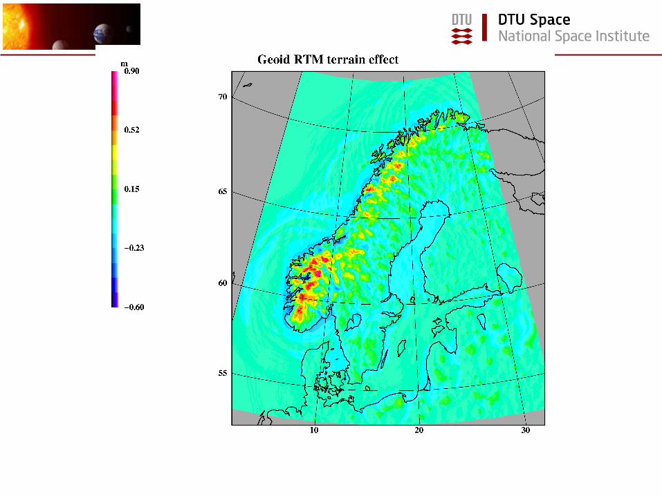
Combining gravity field data and digital terrain models:
Terrain dominates shortwavelength geoid features in mountains
terrain effects to be modelled (remove/restore; prisms, FFT ..)
density known only approximatively (but remove-restore methods robust to errors)
Problems with irregular sampling of terrain with gravity stations
4.50 5.00 5.50 6.00 6.50 7.00 7.50 8.00 8.50 9.00
60.00
60.50
61.00
61.50
62.00
-1200.00
-1000.00
-800.00
-600.00
-400.00
-200.00
0.00
200.00
400.00
600.00
800.00
1000.00
1200.00
1400.00
1600.00
1800.00
2000.00
2200.00
5.00 5.50 6.00 6.50 7.00 7.50 8.00 8.50
60.00
60.50
61.00
61.50
62.00
42.50
43.00
43.50
44.00
44.50
45.00
45.50
46.00
46.50
47.00
47.50
Gravity data and DEM (Sognefjord, Norway) Detailed geoid
Gravimetric geoid determination in mountains
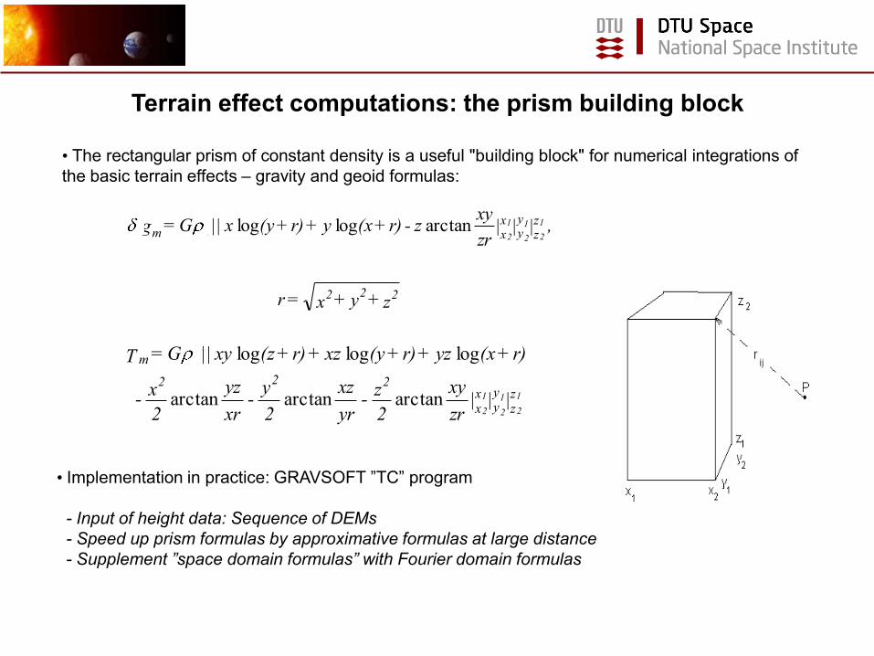
Terrain effect computations: the prism building block
• The rectangular prism of constant density is a useful "building block" for numerical integrations of
the basic terrain effects – gravity and geoid formulas:
z+y+x =r
,|||zr
xyz -r)+(xy + r)+(y x|||G = g
222
zz
yy
xxm
1
2
1
2
1
2arctanloglog
||| zr
xy
2
z -
yr
xz
2
y -
xr
yz
2
x -
r)+(xyz +r)+(yxz + r)+(zxy |||G = T
zz
yy
xx
222
m
1
2
1
2
1
2arctanarctanarctan
logloglog
• Implementation in practice: GRAVSOFT ”TC” program
- Input of height data: Sequence of DEMs
- Speed up prism formulas by approximative formulas at large distance
- Supplement ”space domain formulas” with Fourier domain formulas
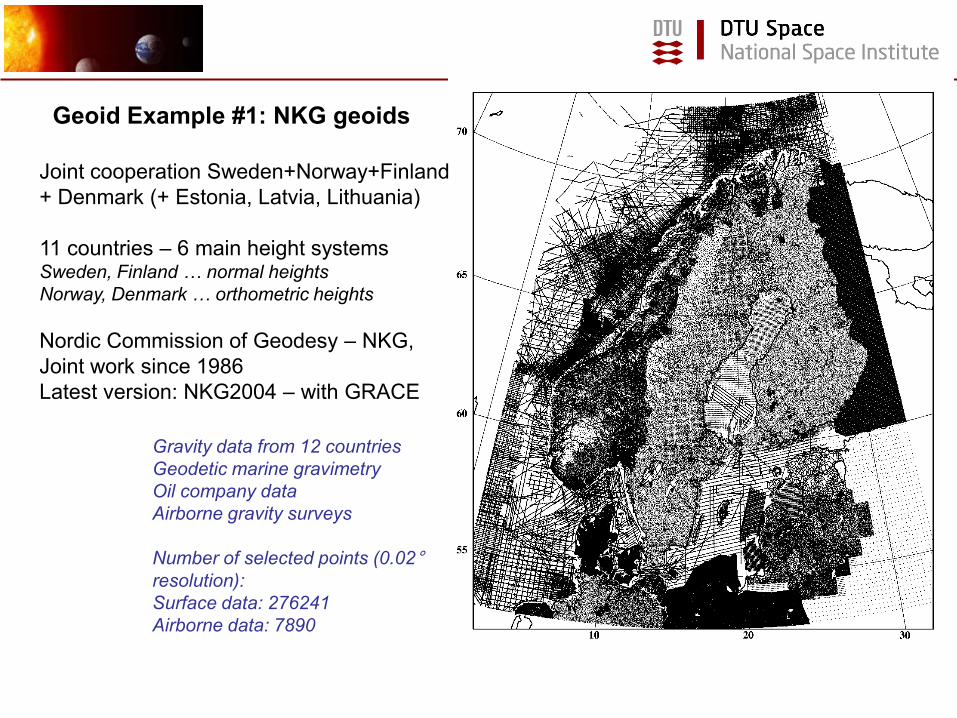
Gravity data from 12 countries
Geodetic marine gravimetry
Oil company data
Airborne gravity surveys
Number of selected points (0.02°resolution):
Surface data: 276241
Airborne data: 7890
Geoid Example #1: NKG geoids
Joint cooperation Sweden+Norway+Finland
+ Denmark (+ Estonia, Latvia, Lithuania)
11 countries – 6 main height systemsSweden, Finland … normal heights
Norway, Denmark … orthometric heights
Nordic Commission of Geodesy – NKG,
Joint work since 1986
Latest version: NKG2004 – with GRACE
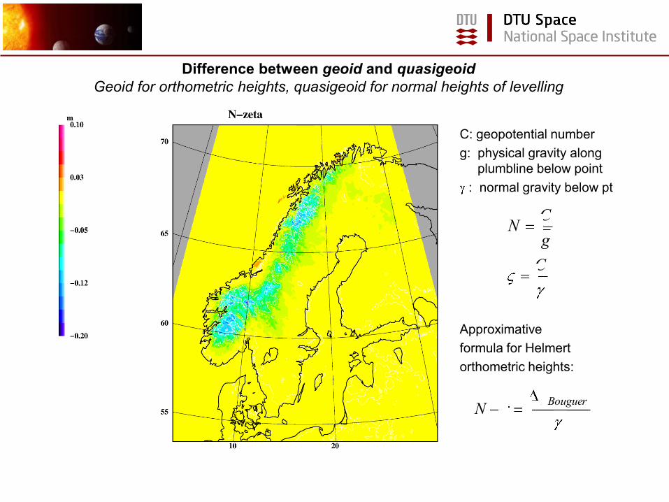
BouguergN
C: geopotential number
g: physical gravity along
plumbline below point
: normal gravity below pt
Approximative
formula for Helmert
orthometric heights:
Difference between geoid and quasigeoid
Geoid for orthometric heights, quasigeoid for normal heights of levelling
C
g
CN
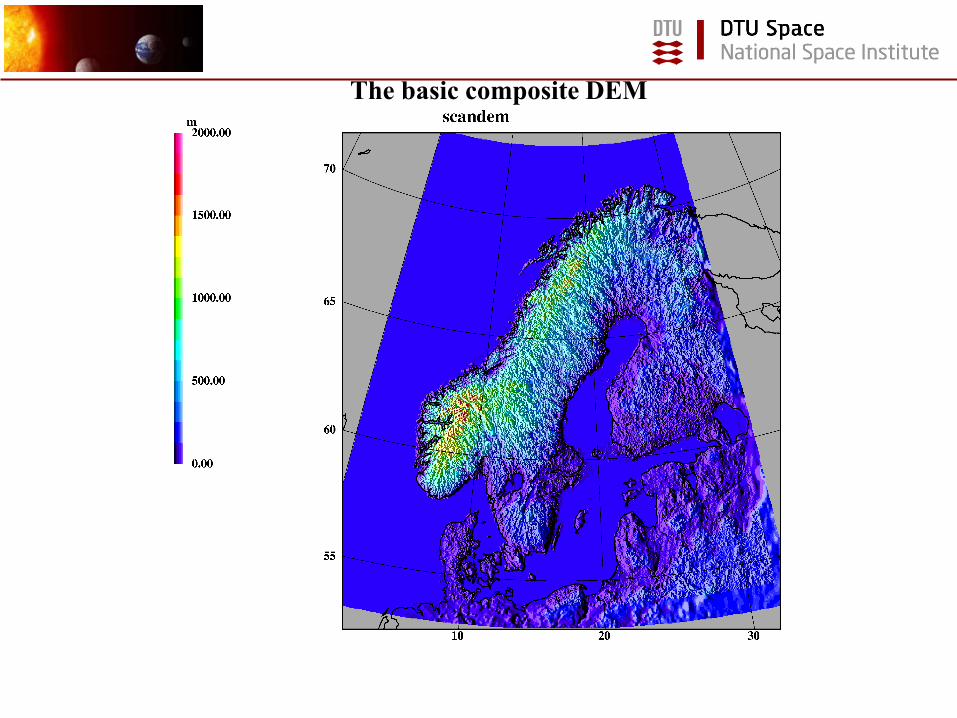
The basic composite DEM

unit: mgal mean std.dev. min. max.
free-air anomalies
(surface data)
-0.85 25.15 -141.17 205.58
- EGM96 -1.13 15.48 -178.93 132.34
- EGM96-RTM 0.37 9.68 -104.49 90.01
airborne data
(Baltic/Skagerrak)
-14.00 19.82 -80.38 48.89
- EGM96 1.56 9.88 -34.12 48.61
- EGM96-RTM 2.07 9.78 -32.46 50.75
Statistics of data reductions – “remove steps”
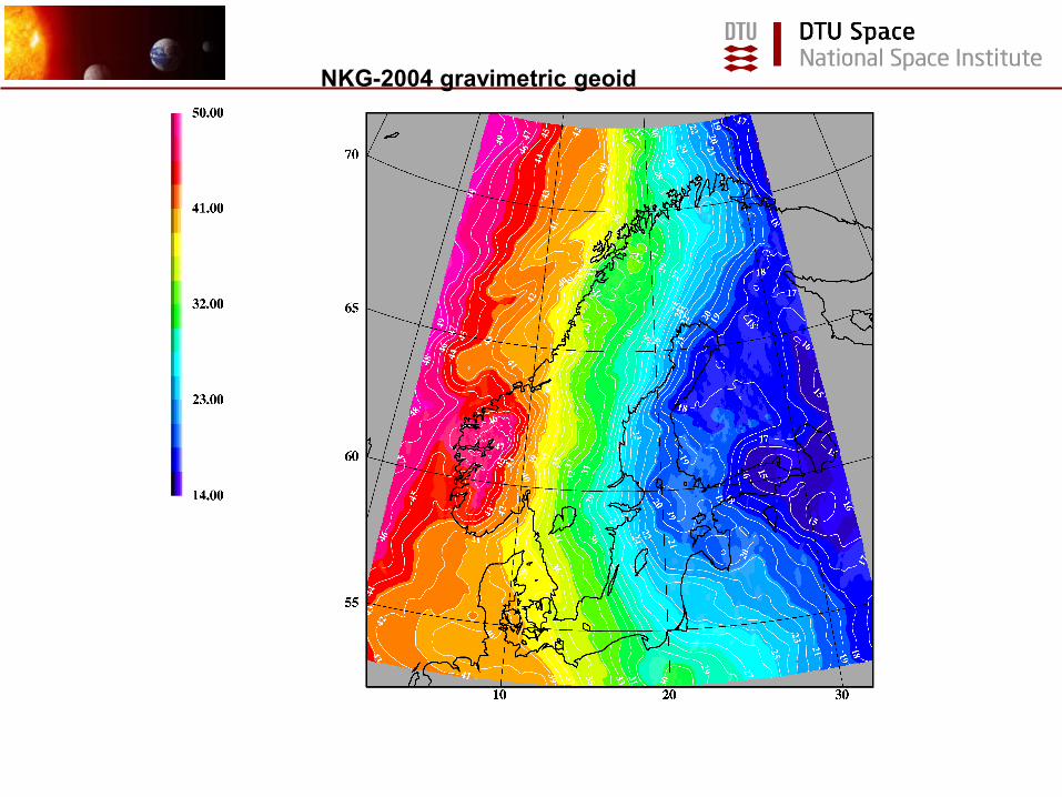
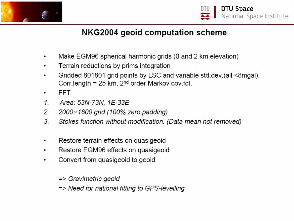
NKG-2004 gravimetric geoid
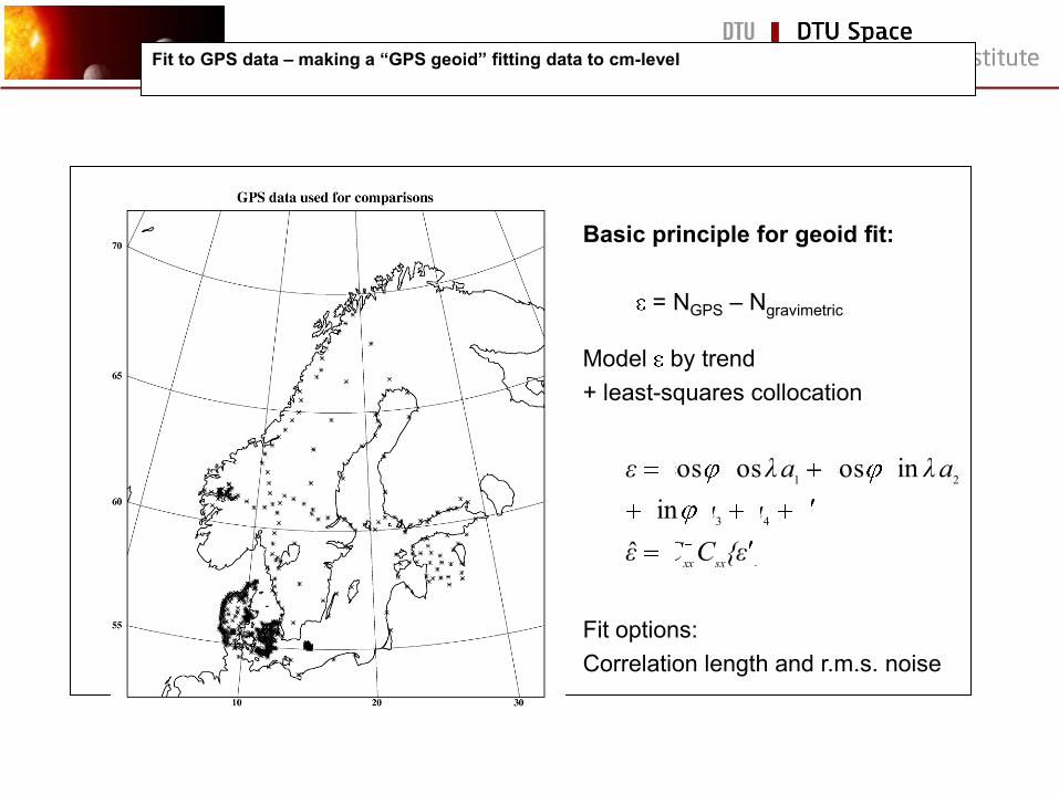
Fit to GPS data – making a “GPS geoid” fitting data to cm-level
Basic principle for geoid fit:
= NGPS – Ngravimetric
Model by trend
+ least-squares collocation
Fit options:
Correlation length and r.m.s. noise
}ˆ
sin
sincoscoscos
1
43
21
ε{CCε
εaa
aλaλε
sxxx
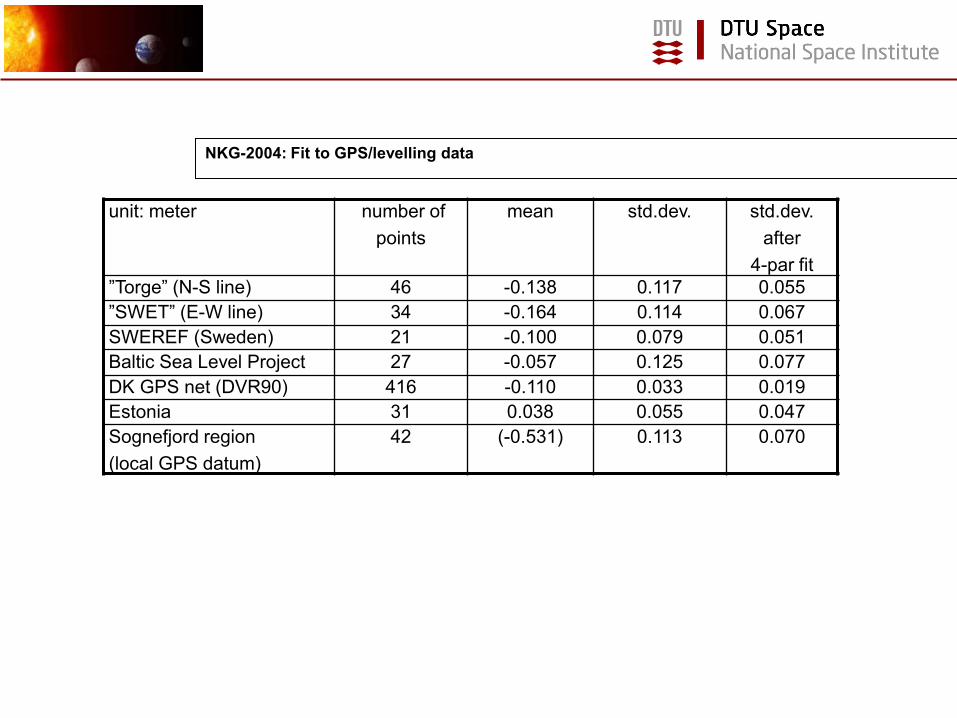
NKG-2004: Fit to GPS/levelling data
unit: meter number of
points
mean std.dev. std.dev.
after
4-par fit
”Torge” (N-S line) 46 -0.138 0.117 0.055
”SWET” (E-W line) 34 -0.164 0.114 0.067
SWEREF (Sweden) 21 -0.100 0.079 0.051
Baltic Sea Level Project 27 -0.057 0.125 0.077
DK GPS net (DVR90) 416 -0.110 0.033 0.019
Estonia 31 0.038 0.055 0.047
Sognefjord region
(local GPS datum)
42 (-0.531) 0.113 0.070
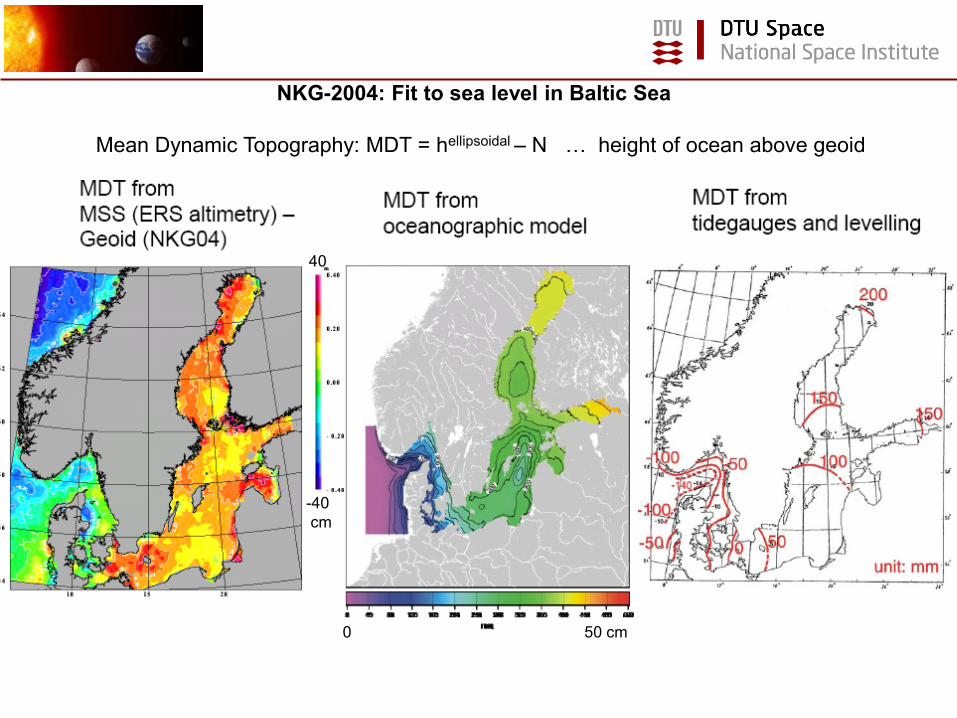
NKG-2004: Fit to sea level in Baltic Sea
Mean Dynamic Topography: MDT = hellipsoidal – N … height of ocean above geoid
0 50 cm
-40
cm
40
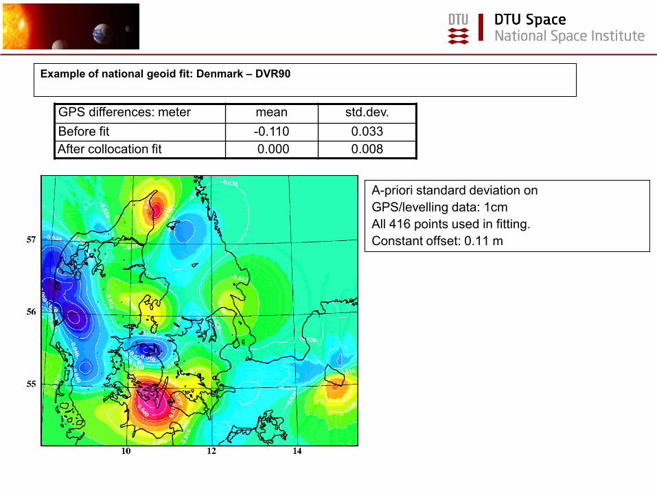
Example of national geoid fit: Denmark – DVR90
A-priori standard deviation on
GPS/levelling data: 1cm
All 416 points used in fitting.
Constant offset: 0.11 m
GPS differences: meter mean std.dev.
Before fit -0.110 0.033
After collocation fit 0.000 0.008

Top Related