Neutrosophic Sets and Systems, Vol. 2, 2014

Rıdvan Şahin, Neutrosophic Hierarchical Clustering Algoritms

Neutrosophic Hierarchical Clustering Algoritms

Rıdvan Şahin

Department of Mathematics, Faculty of Science, Ataturk University, Erzurum, 25240, Turkey. mat.ridone@gmail.com

Abstract. Interval neutrosophic set (INS) is a generaliza-

tion of interval valued intuitionistic fuzzy set (IVIFS),

whose the membership and non-membership values of el-

ements consist of fuzzy range, while single valued neutro-

sophic set (SVNS) is regarded as extension of intuition-

istic fuzzy set (IFS). In this paper, we extend the hierar-

chical clustering techniques proposed for IFSs and IVIFSs

to SVNSs and INSs respectively. Based on the traditional

hierarchical clustering procedure, the single valued neu-

trosophic aggregation operator, and the basic distance

measures between SVNSs, we define a single valued neu-

trosophic hierarchical clustering algorithm for clustering

SVNSs. Then we extend the algorithm to classify an inter-

val neutrosophic data. Finally, we present some numerical

examples in order to show the effectiveness and availabil-

ity of the developed clustering algorithms.

Keywords: Neutrosophic set, interval neutrosophic set, single valued neutrosophic set, hierarchical clustering, neutrosophic aggre-

gation operator, distance measure.

1 Introduction

Clustering is an important process in data mining, pat-

tern recognition, machine learning and microbiology analy-

sis [1, 2, 14, 15, 21]. Therefore, there are various types of techniques for clustering data information such as numerical

information, interval-valued information, linguistic infor-mation, and so on. Several of them are clustering algorithms

such as partitional, hierarchical, density-based, graph-based,

model-based. To handle uncertainty, imprecise, incomplete, and inconsistent information which exist in real world,

Smarandache [3, 4] proposed the concept of neutrosophic set (NS) from philosophical point of view. A neutrosophic

set [3] is a generalization of the classic set, fuzzy set [13], intuitionistic fuzzy set [11] and interval valued intuitionistic

fuzzy set [12]. It has three basic components independently

of one another, which are truht-membership, indeterminacy-membership, and falsity-membership. However, the neutro-

sophic sets is be diffucult to use in real scientiffic or engi-neering applications. So Wang et al. [5, 6] defined the con-

cepts of single valued neutrosophic set (SVNS) and interval

neutrosophic set (INS) which is an instance of a neutro-sophic set. At present, studies on the SVNSs and INSs is

progressing rapidly in many different aspects [7, 8, 9, 10, 16, 18]. Yet, until now there has been little study on clustering

the data represented by neutrosophic information [9]. There-fore, the existing clustering algorithms cannot cluster the

neutrosophic data, so we need to develop some new tech-

niques for clustering SVNSs and INSs.

2 Preliminaries

In this section we recall some definitions, operations and properties regarding NSs, SVNSs and INSs, which will be

used in the rest of the paper.

2.1 Neutrosophic sets

Definition 1. [3] Let 𝑋 be a space of points (objects) and

𝑥 ∈ 𝑋 . A neutrosophic set 𝑁 in 𝑋 is characterized by a truth-membership function 𝑇𝑁, an indeterminacy-member-

ship function 𝐼𝑁 and a falsity-membership function 𝐹𝑁 , where 𝑇𝑁(𝑥) , 𝐼𝑁(𝑥) and 𝐹𝑁(𝑥) are real standard or non-

standard subsets of ]0−, 1+[. That is, 𝑇𝑁 ∶ 𝑈 →]0−, 1+[, 𝐼𝑁 ∶𝑈 →]0−, 1+[ and 𝐹𝑁 ∶ 𝑈 →]0−, 1+[.

There is no restriction on the sum of 𝑇𝑁(𝑥), 𝐼𝑁(𝑥) and

𝐹𝑁(𝑥), so 0− ≤ sup 𝑇𝑁(𝑥) + sup 𝐼𝑁(𝑥) + sup 𝐹𝑁(𝑥) ≤ 3+.

Neutrosophic sets is difficult to apply in real scientific and engineering applications [5]. So Wang et al. [5] pro-

posed the concept of SVNS, which is an instance of neutro-

sophic set.

2.2 Single valued neutrosophic sets

A single valued neutrosophic set has been defined in [5] as follows:

Definition 2. Let 𝑋 be a universe of discourse. A single val-ued neutrosophic set 𝐴 over 𝑋 is an object having the form:

𝐴 = {⟨𝑥, 𝑢𝐴(𝑥), 𝑤𝐴(𝑥), 𝑣𝐴(𝑥)⟩ ∶ 𝑥 ∈ 𝑋},

where 𝑢𝐴: 𝑋 → [0,1] , 𝑤𝐴: 𝑋 → [0,1] and 𝑣𝐴: 𝑋 → [0,1] with the condition

0 ≤ 𝑢𝐴(𝑥) + 𝑤𝐴(𝑥) + 𝑣𝐴(𝑥) ≤ 3, ∀𝑥 ∈ 𝑋.

The numbers 𝑢𝐴(𝑥) , 𝑤𝐴(𝑥) and 𝑣𝐴(𝑥) denote the de-

gree of truth-membership, indeterminacy membership and falsity-membership of 𝑥 to 𝑋, respectively.

Definition 3. Let 𝐴 and 𝐵 be two single valued neutro-sophic sets,

Neutrosophic Sets and Systems, Vol. 2, 2014

Rıdvan Şahin, Neutrosophic Hierarchical Clustering Algoritms

𝐴 = {⟨𝑥, 𝑢𝐴(𝑥), 𝑤𝐴(𝑥), 𝑣𝐴(𝑥)⟩ ∶ 𝑥 ∈ 𝑋} 𝐵 = {⟨𝑥, 𝑢𝐵 (𝑥), 𝑤𝐵 (𝑥), 𝑣𝐵 (𝑥)⟩ ∶ 𝑥 ∈ 𝑋}

Then we can give two basic operations of 𝐴 and 𝐵 as fol-

lows:

1. 𝐴 + 𝐵 = {< 𝑥, 𝑢𝐴(𝑥) + 𝑢𝐵(𝑥) − 𝑢𝐴(𝑥). 𝑢𝐵(𝑥),

𝑤𝐴(𝑥). 𝑤𝐵(𝑥), 𝑣𝐴(𝑥). 𝑣𝐵(𝑥) >∶ 𝑥 ∈ 𝑋};

2. 𝜆𝐴 = {< 𝑥, 1 − (1 − 𝑢𝐴(𝑥))𝜆

, (𝑤𝐴(𝑥))𝜆

, (𝑣𝐴(𝑥))𝜆

>:

𝑥 ∈ 𝑋 and 𝜆 > 0}

Definition 4. Let 𝑋 = {𝑥1, 𝑥2, … , 𝑥𝑛} be a universe of dis-course. Consider that the elements 𝑥𝑖 (i = 1,2,...,n) in the

universe 𝑋 may have different importance, let 𝜔 =(𝜔1, 𝜔2, . . . , 𝜔𝑛)𝑇 be the weight vector of 𝑥𝑖 (i = 1,2,...,n), with 𝜔𝑖 ≥ 0, i = 1,2,...,n, ∑ 𝜔𝑖𝑛

𝑖=1 = 1. Assume that

𝐴 = {⟨𝑥, 𝑢𝐴(𝑥), 𝑤𝐴(𝑥), 𝑣𝐴(𝑥)⟩: 𝑥 ∈ 𝑋} and 𝐵 = {⟨𝑥, 𝑢𝐵(𝑥), 𝑤𝐵(𝑥), 𝑣𝐵(𝑥)⟩: 𝑥 ∈ 𝑋}

be two SVNSs. Then we give the following distance

measures: The weighted Hamming distance and normalized Hamming

distance [9]

𝑒1𝜔(𝐴, 𝐵) = (

1

3∑ 𝜔𝑖(|𝑢𝐴(𝑥𝑖) − 𝑢𝐵(𝑥𝑖)| + |𝑤𝐴(𝑥𝑖) − 𝑤𝐵(𝑥𝑖)| +𝑛

𝑖=1

|𝑣𝐴(𝑥𝑖) − 𝑣𝐵(𝑥𝑖)|)). (1)

Assume that 𝜔 = (1 𝑛⁄ , 1 𝑛⁄ , . . . , 1 𝑛⁄ )𝑇, then Eq. (1) is re-

duced to the normalized Hamming distance

𝑒2𝑛(𝐴, 𝐵) = (

1

3𝑛∑ (|𝑢𝐴(𝑥𝑖) − 𝑢𝐵(𝑥𝑖)| + |𝑤𝐴(𝑥𝑖) − 𝑤𝐵(𝑥𝑖)| +𝑛

𝑖=1

|𝑣𝐴(𝑥𝑖) − 𝑣𝐵(𝑥𝑖)|)) (2)

The weighted Euclidean distance and normalized Euclidean distance [7]

𝑒3𝜔(𝐴, 𝐵) = (

1

3∑ 𝜔𝑖(|𝑢𝐴(𝑥𝑖) − 𝑢𝐵(𝑥𝑖)|)2 + (|𝑤𝐴(𝑥𝑖) − 𝑤𝐵(𝑥𝑖)|)2 +𝑛

𝑖=1

(|𝑣𝐴(𝑥𝑖) − 𝑣𝐵(𝑥𝑖)|)2)

1

2 (3)

Assume that ω = (1/n,1/n,...,1/n)T, then Eq. (3) is reduced to the normalized Euclidean distance

𝑒4𝑛(𝐴, 𝐵) = (

1

3𝑛∑ (|𝑢𝐴(𝑥𝑖) − 𝑢𝐵(𝑥𝑖)|)2 + (|𝑤𝐴(𝑥𝑖) −𝑛

𝑖=1

𝑤𝐵(𝑥𝑖)|)2 + (|𝑣𝐴(𝑥𝑖) − 𝑣𝐵(𝑥𝑖)|)2)

1

2 (4)

2.3 Interval neutrosophic sets

Definition 5. [3] Let 𝑋 be a set and Int[0,1] be the set of all closed subsets of [0,1]. An INS �̃� in 𝑋 is defined with the

form

�̃� = {⟨𝑥, 𝑢𝐴(𝑥), 𝑤𝐴(𝑥), 𝑣𝐴(𝑥)⟩ ∶ 𝑥 ∈ 𝑋}

where 𝑢𝐴: 𝑋 → Int[0,1] , 𝑤𝐴: 𝑋 → Int[0,1] and 𝑣𝐴: 𝑋 →

Int[0,1] with the condition

0 ≤ sup 𝑢𝐴(𝑥) + sup 𝑤𝐴(𝑥) + sup 𝑣𝐴(𝑥) ≤ 3, for all 𝑥 ∈ 𝑋.

The intervals 𝑢𝐴(𝑥), 𝑤𝐴(𝑥) and 𝑣𝐴(𝑥) denote the truth-

membership degree, the indeterminacy membership degree and the falsity-membership degree of 𝑥 to �̃�, respectively.

For convenience, if let

𝑢�̃�(𝑥) = [𝑢�̃�+(𝑥), 𝑢�̃�

−(𝑥)]

𝑤�̃�(𝑥) = [𝑤�̃�+(𝑥), 𝑤�̃�

−(𝑥)]

𝑣�̃�(𝑥) = [𝑣�̃�+(𝑥), 𝑣�̃�

−(𝑥)]

then

�̃� = {⟨𝑥, [𝑢�̃�−(𝑥), 𝑢�̃�

+(𝑥)], [𝑤�̃�−(𝑥), 𝑤�̃�

+(𝑥)], [𝑣�̃�−(𝑥), 𝑣�̃�

+(𝑥)]⟩}: 𝑥 ∈ 𝑋}

with the condition

0 ≤ sup 𝑢𝐴+(𝑥) + sup 𝑤𝐴

+(𝑥) + sup 𝑣𝐴+(𝑥) ≤ 3,

for all 𝑥 ∈ 𝑋 . If 𝑤𝐴(𝑥) = [0,0] and sup 𝑢𝐴+(𝑥) +

sup 𝑣𝐴+ ≤ 1 then �̃� reduces to an interval valued intuition-

istic fuzzy set.

Definition 6. [20] Let �̃� and �̃� be two interval neutrosophic

sets,

�̃� = {⟨𝑥, [𝑢�̃�−(𝑥), 𝑢�̃�

+(𝑥)], [𝑤�̃�−(𝑥), 𝑤�̃�

+(𝑥)], [𝑣�̃�−(𝑥), 𝑣�̃�

+(𝑥)]⟩: 𝑥 ∈ 𝑋},

�̃� = {⟨𝑥, [𝑢�̃�−(𝑥), 𝑢�̃�

+(𝑥)], [𝑤�̃�−(𝑥), 𝑤�̃�

+(𝑥)], [𝑣�̃�−(𝑥), 𝑣�̃�

+(𝑥)]⟩: 𝑥 ∈ 𝑋}.

Then two basic operations of �̃� and �̃� are given as follows:

1. �̃� + �̃� = {< 𝑥, [𝑢�̃�−(𝑥) + 𝑢�̃�

−(𝑥)−, 𝑢�̃�+(𝑥) ⋅ 𝑢�̃�

−(𝑥), 𝑢�̃�+(𝑥) +

𝑢�̃�+(𝑥) − 𝑢�̃�

+(𝑥) ⋅ 𝑢�̃�+(𝑥)], [𝑢�̃�

−(𝑥) ⋅ 𝑤�̃�−(𝑥), 𝑤�̃�

+(𝑥) ⋅ 𝑤�̃�+(𝑥)],

[𝑣�̃�−(𝑥) ⋅ 𝑣�̃�

−(𝑥), 𝑣�̃�+(𝑥) ⋅ 𝑣�̃�

+(𝑥)]: 𝑥 ∈ 𝑋}

2. 𝜆�̃� = {< 𝑥, [, 1 − (1 − 𝑢�̃�−(𝑥))

𝜆, 1 − (1 − 𝑢�̃�

+(𝑥))𝜆

] ,

[(𝑤�̃�−(𝑥))

𝜆, (𝑤�̃�

+(𝑥))𝜆

] , [(𝑣�̃�−(𝑥))

𝜆, (𝑣�̃�

+(𝑥))𝜆

] >: 𝑥 ∈ 𝑋 and 𝜆 > 0}.

Definition 7. Let 𝑋 = {𝑥1, 𝑥2, . . . , 𝑥𝑛} be a universe of dis-

course. Consider that the elements 𝑥𝑖 (i = 1,2,...,n) in the uni-verse 𝑋 may have different importance, let 𝜔 =(𝜔1, 𝜔2, . . . , 𝜔𝑛)𝑇 be the weight vector of 𝑥𝑖 (i = 1,2,...,n), with 𝜔𝑖 ≥ 0, i = 1,2,...,n, ∑ 𝜔𝑖

𝑛𝑖=1 = 1. Suppose that �̃� and

�̃� are two interval neutrosophic sets. Ye [6] has defined the

distance measures for INSs as follows: The weighted Hamming distance and normalized Hamming

distance:

𝑑1𝜔(�̃�, �̃�) = (

1

6∑ 𝜔𝑖(|𝑢�̃�

−(𝑥) − 𝑢𝐵−(𝑥)|𝑛

𝑖=1 + |𝑢�̃�+(𝑥) − 𝑢𝐵

+(𝑥)|

+|𝑤�̃�+(𝑥) − 𝑤𝐵

+(𝑥)| + |𝑣�̃�−(𝑥) − 𝑢𝐵

−(𝑥)| + |𝑣�̃�+(𝑥) − 𝑢𝐵

+(𝑥)|) (5)

Assume that 𝜔 = (1 𝑛⁄ , 1 𝑛⁄ , . . . , 1 𝑛⁄ )𝑇, then Eq. (5) is re-duced to the normalized Hamming distance

𝑑2𝜔(�̃�, �̃�) = (

1

6𝑛∑ (|𝑢�̃�

−(𝑥) − 𝑢�̃�−(𝑥)|𝑛

𝑖=1 +

|𝑢�̃�+(𝑥) − 𝑢�̃�

+(𝑥)| + |𝑤�̃�+(𝑥) − 𝑤�̃�

+(𝑥)| + |𝑣�̃�−(𝑥) − 𝑢�̃�

−(𝑥)| +

Neutrosophic Sets and Systems, Vol. 2, 2014

Rıdvan Şahin, Neutrosophic Hierarchical Clustering Algoritms

|𝑣�̃�+(𝑥) − 𝑢�̃�

+(𝑥)|) (6)

The weighted Euclidean distance and normalized Hamming distance

𝑑3𝜔(�̃�, �̃�) = (

1

6∑ 𝜔𝑖(|𝑢�̃�

−(𝑥) − 𝑢�̃�−(𝑥)|

2𝑛𝑖=1 + |𝑢�̃�

+(𝑥) − 𝑢�̃�+(𝑥)|

2+

|𝑤�̃�−(𝑥) − 𝑤�̃�

−(𝑥)|2

+ |𝑤�̃�+(𝑥) − 𝑤�̃�

+(𝑥)|2

+ |𝑣�̃�−(𝑥) − 𝑢�̃�

−(𝑥)|2

+

|𝑣𝐴+(𝑥) − 𝑢𝐵

+(𝑥)|2))

1

2 (7)

Assume that 𝜔 = (1/𝑛, 1/𝑛, . . . ,1/𝑛)𝑇, then Eq. (7) is re-

duced to the normalized Hamming distance

𝑑4𝑛(�̃�, �̃�) = (

1

6𝑛∑ (|𝑢�̃�

−(𝑥) − 𝑢�̃�−(𝑥)|

2𝑛𝑖=1 + |𝑢�̃�

+(𝑥) − 𝑢�̃�+(𝑥)|

2+

|𝑤�̃�−(𝑥) − 𝑤�̃�

−(𝑥)|2

+ |𝑤�̃�+(𝑥) − 𝑤�̃�

+(𝑥)|2

+ |𝑣�̃�−(𝑥) − 𝑢�̃�

−(𝑥)|2

+

|𝑣�̃�+(𝑥) − 𝑢�̃�

+(𝑥)|2))

1

2 (8)

Definition 8. [20] Let

�̃�𝑘 = ⟨[𝑢�̃�−(𝑥), 𝑢�̃�

+(𝑥)], [𝑤�̃�−(𝑥), 𝑤�̃�

+(𝑥)], [𝑣�̃�−(𝑥), 𝑣�̃�

+(𝑥)]⟩

𝑘 = 1,2, … , . 𝑛) be a collection of interval neutrosophic sets. A mapping �̃�𝜔 ∶ 𝐼𝑁𝑆𝑛 → 𝐼𝑁𝑆 is called an interval neutro-

sophic weighted averaging operator of dimension 𝑛 if it is

satisfies

�̃�𝜔(�̃�1, �̃�2, … , �̃�𝑛) = ∑ 𝜔𝑘�̃�𝑘𝑛𝑘=1

where 𝜔 = (𝜔1, 𝜔2, . . . , 𝜔𝑛)𝑇 is the weight vector of �̃�𝑘 (𝑘 =

1,2, . . . , 𝑛), 𝜔𝑘 ∈ [0,1] and ∑ 𝜔𝑘 = 1𝑛𝑘=1 .

Theorem 1. [20] Suppose that

�̃�𝑘 = ⟨[𝑢𝐴−(𝑥), 𝑢𝐴

+(𝑥)], [𝑤𝐴−(𝑥), 𝑤𝐴

+(𝑥)], [𝑣𝐴−(𝑥), 𝑣𝐴

+(𝑥)]⟩

𝑘 = 1,2, … , . 𝑛) are interval neutrosophic sets. Then the ag-gregation result through using the interval neutrosophic

weighted averaging operator Fω is an interval neutrosophic set and

�̃�𝜔(�̃�1, �̃�2, … , �̃�𝑛) = �̃�𝑘

=< [1 − ∏ (1 − 𝑢�̃�𝑘

− (𝑥))𝜔𝑘

, 1 − ∏ (1 − 𝑢�̃�𝑘

+ (𝑥))𝜔𝑘

𝑛𝑘=1

𝑛𝑘=1 ],

[∏ (𝑤�̃�𝑘

− (𝑥))𝜔𝑘

, ∏ (𝑤�̃�𝑘

+ (𝑥))𝜔𝑘

𝑛𝑘=1

𝑛𝑘=1 ],

[∏ (𝑣�̃�𝑘

− (𝑥))𝜔𝑘

, ∏ (𝑣�̃�𝑘

+ (𝑥))𝜔𝑘

𝑛𝑘=1

𝑛𝑘=1 ] > (9)

where 𝜔 = (𝜔1, 𝜔2, . . . , 𝜔𝑛)𝑇 is the weight vector of �̃�𝑘

(𝑘 = 1,2, . . . , 𝑛), 𝜔𝑘 ∈ [0,1] and ∑ 𝜔𝑘 = 1.𝑛𝑘=1

Suppose that 𝜔 = (1/𝑛, 1/𝑛, . . . ,1/𝑛)𝑇 then the �̃�𝜔 is called an arithmetic average operator for INSs.

Since INS is a generalization of SVNS, according to Defi-nition 8 and Theorem 1, the single valued neutrosophic

weighted averaging operator can be easily obtained as fol-lows.

Definition 9. Let 𝐴𝑘 = ⟨𝑢𝐴𝑘

, 𝑤𝐴𝑘, 𝑣𝐴𝑘

⟩

(𝑘 = 1,2, . . . , 𝑛) be a collection single valued neutro-

sophic sets. A mapping 𝐹𝜔 ∶ 𝑆𝑉𝑁𝑆𝑛 → 𝑆𝑉𝑁𝑆 is called a

single valued neutrosophic weighted averaging operator of

dimension 𝑛 if it is satisfies

𝐹𝜔 (𝐴1, 𝐴2, . . . , 𝐴𝑛) = ∑ 𝜔𝑘𝐴𝑘𝑛𝑘=1

where 𝜔 = (𝜔1, 𝜔2, … , 𝜔𝑛)𝑇 is the weight vector of

𝐴𝑘(𝑘 = 1,2, . . . , 𝑛), 𝜔𝑘 ∈ [0,1] and ∑ 𝜔𝑘 = 1𝑛𝑘=1 .

Theorem 2. Suppose that

𝐴𝑘 = ⟨𝑢𝐴𝑘, 𝑤𝐴𝑘

, 𝑣𝐴𝑘⟩

(𝑘 = 1,2, . . . , 𝑛) are single valued neutrosophic sets. Then

the aggregation result through using the single valued neu-trosophic weighted averaging operator 𝐹𝜔 is single neutro-

sophic set and

𝐹𝜔 (𝐴1, 𝐴2, . . . , 𝐴𝑛) = 𝐴𝑘

=< 1 − ∏ (1 − 𝑢𝐴𝑘(𝑥))

𝜔𝑘

,𝑛𝑘=1

∏ (𝑤𝐴𝑘(𝑥))

𝜔𝑘

,𝑛𝑘=1 ∏ (𝑣𝐴𝑘

(𝑥))𝜔𝑘

>𝑛𝑘=1 (10)

where 𝜔 = (𝜔1, 𝜔2, … , 𝜔𝑛)𝑇 is the weight vector of 𝐴𝑘(𝑘 = 1,2, . . . , 𝑛), 𝜔𝑘 ∈ [0,1] and ∑ 𝜔𝑘 = 1𝑛

𝑘=1 .

Suppose that 𝜔 = (1/𝑛, 1/𝑛, … ,1/𝑛)𝑇 , then the 𝐹𝜔 is

called an arithmetic average operator for SVNSs.

3 Neutrosophic hierarchical algorithms

The traditional hierarchical clustering algorithm [17, 19] is generally used for clustering numerical information.

By extending the traditional hierarchical clustering algo-

rithm, Xu [22] introduced an intuitionistic fuzzy hierar-chical clustering algorithm for clustering IFSs and extended

it to IVIFSs. However, they fail to deal with the data infor-mation expressed in neutrosophic environment. Based on

extending the intuitionistic fuzzy hierarchical clustering al-

gorithm and its extended form, we propose the neutrosophic hierarchical algorithms which are called the single valued

neutrosophic hierarchical clustering algorithm and interval neutrosophic hierarchical clustering algorithm.

Algorithm 1. Let us consider a collection of n SVNSs

𝐴𝑘(𝑘 = 1,2, . . . , 𝑛). In the first stage, the algorithm starts by assigning each of the n SVNSs to a single cluster. Based

on the weighted Hamming distance (1) or the weighted Eu-clidean distance (3), the SVNSs 𝐴𝑘(𝑘 = 1,2, . . . , 𝑛) are

then compared among themselves and are merged them into a single cluster according to the closest (with smaller dis-

tance) pair of clusters. The process are continued until all

the SVNSs 𝐴𝑘 are merged into one cluster i.e., clustered into a single cluster of size n. In each stage, only two clusters can

be merged and they cannot be separated after they are merged, and the center of each cluster is recalculated by us-

ing the arithmetic average (from Eq. (10)) of the SVNSs

proposed to the cluster. The distance between the centers of

Neutrosophic Sets and Systems, Vol. 2, 2014

Rıdvan Şahin, Neutrosophic Hierarchical Clustering Algoritms

each cluster is considered as the distance between two clus-

ters.

However, the clustering algorithm given above cannot

cluster the interval neutrosophic data. Therefore, we need

another clustering algorithm to deal with the data repre-sented by INSs.

Algorithm 2. Let us consider a collection of n INSs �̃�𝑘(𝑘 = 1,2, . . . , 𝑛). In the first stage, the algorithm starts

by assigning each of the n INSs to a single cluster. Based on

the weighted Hamming distance (5) or the weighted Euclid-ean distance (7), the INSs �̃�𝑘(𝑘 = 1,2, . . . , 𝑛) are then

compared among themselves and are merged them into a single cluster according to the closest (with smaller dis-

tance) pair of clusters. The process are continued until all the INSs �̃�𝑘 are merged into one cluster i.e., clustered into a

single cluster of size n. In each stage, only two clusters can

be merged and they cannot be separated after they are merged, and the center of each cluster is recalculated by us-

ing the arithmetic average (from Eq. (9)) of the INSs pro-posed to the cluster. The distance between the centers of

each cluster is considered as the distance between two clus-

ters.

3.1 Numerical examples.

Let us consider the clustering problem adapted from [21].

Example 1. Assume that five building materials: sealant, floor varnish, wall paint, carpet, and polyvinyl chloride

flooring, which are represented by the SVNSs 𝐴𝑘(𝑘 = 1,2, . . . ,5) in the feature space 𝑋 = {𝑥1, 𝑥2, . . . , 𝑥8}. 𝜔 = (0.15,0.10,0.12,0.15,0.10,0.13,0.14,0.11) is the

weight vector of 𝑥𝑖(𝑖 = 1,2, . . . ,8), and the given data are listed as follows:

𝐴1 = {(𝑥1 ,0.20,0.05,0.50), (𝑥2, 0.10,0.15,0.80), (𝑥3 ,0.50,0.05,0.30), (𝑥4, 0.90,0.55,0.00), (𝑥5 ,0.40,0.40,0.35), (𝑥6, 0.10,0.40,0.90), (𝑥7 ,0.30,0.15,0.50), (𝑥8, 1.00,0.60,0.00), }

𝐴2 = {(𝑥1, 0.50,0.60,0.40), (𝑥2, 0.60,0.30,0.15)}, (𝑥3, 1.00,0.60,0.00), (𝑥4, 0.15,0.05,0.65), (𝑥5, 0.00,0.25,0.80), (𝑥6, 0.70,0.65,0.15), (𝑥7, 0.50,0.50,0.30), (𝑥8, 0.65,0.05,0.20)}

𝐴3 = {(𝑥1, 0.45,0.05,0.35), (𝑥2, 0.60,0.50,0.30)}, (𝑥3, 0.90,0.05,0.00), (𝑥4, 0.10,0.60,0.80), (𝑥5, 0.20,0.35,0.70), (𝑥6, 0.60,0.40,0.20), (𝑥7, 0.15,0.05,0.80), (𝑥8, 0.20,0.60,0.65)}

𝐴4 = {(𝑥1, 1.00,0.65,0.00), (𝑥2, 1.00,0.25,0.00)}, (𝑥3, 0.85,0.65,0.10), (𝑥4, 0.20,0.05,0.80), (𝑥5, 0.15,0.30,0.85), (𝑥6, 0.10,0.60,0.70), (𝑥7, 0.30,0.60,0.70), (𝑥8, 0.50,0.35,0.70)}

𝐴5 = {(𝑥1, 0.90,0.20,0.00), (𝑥2, 0.90,0.40,0.10), (𝑥3, 0.80,0.05,0.10), (𝑥4, 0.70,0.45,0.20), (𝑥5, 0.50,0.25,0.15), (𝑥6, 0.30,0.30,0.65), (𝑥7, 0.15,0.10,0.75), (𝑥8, 0.65,0.50,0.80)}

Now we utilize Algorithm 1 to classify the building ma-

terials 𝐴𝑘(𝑘 = 1,2, . . . ,5):

Step1 In the first stage, each of the SVNSs 𝐴𝑘(𝑘 = 1,2, . . . ,5) is considered as a unique cluster {𝐴1}, {𝐴2}, {𝐴3}, {𝐴4}, {𝐴5}.

Step2 Compare each SVNS 𝐴𝑘 with all the other four

SVNSs by using Eq. (1):

𝑒1𝜔(𝐴1, 𝐴2) = 𝑑1 (𝐴2, 𝐴1) = 0.6403

𝑒1𝜔(𝐴1, 𝐴3) = 𝑑1 (𝐴3, 𝐴1) = 0.5191

𝑒1𝜔(𝐴1, 𝐴4) = 𝑑1 (𝐴4, 𝐴1) = 0.7120

𝑒1𝜔(𝐴1, 𝐴5) = 𝑑1 (𝐴5, 𝐴1) = 0.5435

𝑒1𝜔(𝐴2, 𝐴3) = 𝑑1 (𝐴3, 𝐴2) = 0.5488

𝑒1𝜔(𝐴2, 𝐴4) = 𝑑1 (𝐴4, 𝐴2) = 0.4546

𝑒1𝜔(𝐴2, 𝐴5) = 𝑑1 (𝐴5, 𝐴2) = 0.6775

𝑒1𝜔(𝐴3, 𝐴4) = 𝑑1 (𝐴4, 𝐴3) = 0.3558

𝑒1𝜔(𝐴3, 𝐴5) = 𝑑1 (𝐴5, 𝐴3) = 0.2830

𝑒1𝜔(𝐴4, 𝐴5) = 𝑑1 (𝐴5, 𝐴4) = 0.3117

and hence 𝑒1

𝜔(𝐴1, 𝐴3) = min{𝑒1

𝜔(𝐴1, 𝐴2), 𝑒1𝜔(𝐴1, 𝐴3) , 𝑒1

𝜔(𝐴1, 𝐴4), 𝑒1𝜔(𝐴1, 𝐴5)}

= 0.5191,

𝑒1𝜔(𝐴2, 𝐴4) =

min{𝑒1𝜔(𝐴2, 𝐴1), 𝑒1

𝜔(𝐴2, 𝐴3) , 𝑒1𝜔(𝐴2, 𝐴4), 𝑒1

𝜔(𝐴2, 𝐴5)} = 0.4546,

𝑒1𝜔(𝐴3, 𝐴5) =

min{𝑒1𝜔(𝐴3, 𝐴1), 𝑒1

𝜔(𝐴3, 𝐴2) , 𝑒1𝜔(𝐴3, 𝐴4), 𝑒1

𝜔(𝐴3, 𝐴5)} = 0.2830.

Then since only two clusters can be merged in each stage,

the SVNSs 𝐴𝑘(𝑘 = 1,2, . . . ,5) can be clustered into the fol-lowing three clusters at the second stage {𝐴1}, {𝐴2, 𝐴4}, {𝐴3, 𝐴5 }.

Step3 Calculate the center of each cluster by using Eq. (10)

𝑐{𝐴1} = 𝐴1

𝑐{𝐴2, 𝐴4} = 𝐹𝜔(𝐴2, 𝐴4) = {(𝑥1, 1.00,0.62,0.00), (𝑥2, 1.00,0.27,0.00),

(𝑥3, 1.00,0.62,0.00), (𝑥4, 0.17,0.05,0.72), (𝑥5, 0.07,0.27,0.82), (𝑥6, 0.48,0.62,0.32), (𝑥7, 0.40,0.54,0.45), (𝑥8, 0.58,0.13,0.37)}

𝑐{𝐴3, 𝐴5} = 𝐹𝜔(𝐴3, 𝐴5) = {(𝑥1, 0.76,0.10,0.00), (𝑥2, 0.80,0.44,0.17),

(𝑥3, 0.85,0.05,0.00), (𝑥4, 0.48,0.51,0.40), (𝑥5, 0.36,0.29,0.32), (𝑥6, 0.47,0.34,0.36), (𝑥7, 0.15,0.07,0.77), (𝑥8, 0.47,0.54,0.72)}.

Neutrosophic Sets and Systems, Vol. 2, 2014

Rıdvan Şahin, Neutrosophic Hierarchical Clustering Algoritms

and then compare each cluster with the other two clus-

ters by using Eq. (1):

𝑒1𝜔(𝑐{𝐴1}, 𝑐{𝐴2, 𝐴4}) = 𝑒1

𝜔(𝑐{𝐴2, 𝐴4}, 𝑐{𝐴1}) = 0.7101,

𝑒1𝜔(𝑐{𝐴1}, 𝑐{𝐴3, 𝐴5}) = 𝑒1

𝜔(𝑐{𝐴3, 𝐴5}, 𝑐{𝐴1}) = 5266,

𝑒1𝜔(𝑐{𝐴2, 𝐴4}, 𝑐{𝐴3, 𝐴5}) = 𝑒1

𝜔(𝑐{𝐴3, 𝐴5}, 𝑐{𝐴2, 𝐴4})

= 0.4879.

Subsequently, the SVNSs 𝐴𝑘(𝑘 = 1,2, . . . ,5) can be

clustered into the following two clusters at the third

stage {𝐴1}, {𝐴2, 𝐴3, 𝐴4, 𝐴5 }.

Finally, the above two clusters can be further clustered

into a unique cluster {𝐴1, 𝐴2, 𝐴3, 𝐴4, 𝐴5 }.

All the above processes can be presented as in Fig. 1.

FIGURE 1: Classification of the building materi-

als 𝐴𝑘(𝑘 = 1,2, . . . ,5)

Example 2. Consider four enterprises, represented by

the INSs �̃�𝑘(𝑘 = 1,2,3,4) in the attribute set 𝑋 =

{𝑥1, 𝑥2, . . . , 𝑥6} , where (1) 𝑥1−the ability of sale; (2)

𝑥2−the ability of management; (3) 𝑥3−the ability of

production; (4) 𝑥4 −the ability of technology; (5)

𝑥5−the ability of financing; (6) 𝑥6−the ability of risk

bearing (the weight vector of 𝑥𝑖(𝑖 = 1,2, . . . ,6) is 𝜔 =

(0.25,0.20,15,0.10,0.15,0.15) . The given data are

listed as follows.

�̃�1 = {(𝑥1, [0.70,0.75], [0.25,0.45], [0.10,0.15]),

(𝑥2, [0.00,0.10], [0.15,0.15], [0.80,0.90]),

(𝑥3, [0.15,0.20], [0.05,0.35], [0.60,0.65]),

(𝑥4, [0.50,0.55], [0.45,0.55], [0.30,0.35]),

(𝑥5, [0.10,0.15], [0.40,0.60], [0.50,0.60]),

(𝑥6, [0.70,0.75], [0.20,0.25], [0.10,0.15])}

�̃�2 = (𝑥1, [0.40,0.45], [0.00,0.15], [0.30,0.35]),

(𝑥2, [0.60,0.65], [0.10,0.25], [0.20,0.30]),

(𝑥3, [0.80,1.00], [0.05,0.75], [0.00,0.00]),

(𝑥4, [0.70,0.90], [0.35,0.65], [0.00,1.00]),

(𝑥5, [0.70,0.75], [0.15,0.55], [0.10,0.20]),

(𝑥6, [0.90,1.00], [0.30,0.35], [0.00,0.00])}.

�̃�3 = (𝑥1, [0.20,0.30], [0.85,0.60], [0.40,0.45),

(𝑥2, [0.80,0.90], [0.10,0.25], [0.00,0.10]),

(𝑥3, [0.10,0.20], [0.00,0.05], [0.70,0.80]),

(𝑥4, [0.15,0.20], [0.25,0.45], [0.70,0.75]),

(𝑥5, [0.00,0.10], [0.25,0.35], [0.80,0.90]),

(𝑥6, [0.60,0.70], [0.15,0.25], [0.20,0.30])}.

�̃�4 = (𝑥1, [0.60,0.65], [0.05,0.10], [0.30,0.35]),

(𝑥2, [0.45,0.50], [0.45,0.55], [0.30,0.40]),

(𝑥3, [0.20,0.25], [0.05,0.25], [0.65,0.70]),

(𝑥4, [0.20,0.30], [0.35,0.45], [0.50,0.60]),

(𝑥5, [0.00,0.10], [0.35,0.75], [0.75,0.80]),

(𝑥6, [0.50,0.60], [0.00,0.05], [0.20,0.25])}.

Here Algorithm 2 can be used to classify the enter-

prises�̃�𝑘(𝑘 = 1,2,3,4):

Step 1 In the first stage, each of the INSs �̃�𝑘(𝑘 =

1,2,3,4) is considered as a unique cluster

{�̃�1}, {�̃�2}, {�̃�3}, {�̃�4}

Step 2 Compare each INS �̃�𝑘 with all the other three

INSs by using Eq. (5)

𝑑1𝜔(�̃�1, �̃�2) = 𝑑1

𝜔(�̃�2, �̃�1) = 0.3337,

𝑑1𝜔(�̃�1, �̃�3) = 𝑑1

𝜔(�̃�3, �̃�1) = 0.2937,

𝑑1𝜔(�̃�1, �̃�4) = 𝑑1

𝜔(�̃�4, �̃�1) = 0.2041,

𝑑1𝜔(�̃�2, �̃�3) = 𝑑1

𝜔(�̃�3, �̃�2) = 0.3508,

𝑑1𝜔(�̃�2, �̃�4) = 𝑑1

𝜔(�̃�4, �̃�2) = 0.2970,

𝑑1𝜔(�̃�3, �̃�4) = 𝑑1

𝜔(�̃�4, �̃�3) = 0.2487,

then the INSs �̃�𝑘(𝑘 = 1,2,3,4) can be clustered into

the following three clusters at the second stage

{�̃�1, �̃�4}, {�̃�2}, {�̃�3}.

Step 3 Calculate the center of each cluster by using Eq.

(9)

𝑐{�̃�2} = {�̃�2}, 𝑐{�̃�3} = {�̃�3},

𝑐{�̃�1, �̃�4} = 𝐹𝜔(�̃�1, �̃�4) =

(𝑥1, [0.60,0.70], [0.11,0.21], [0.17,0.22]),

(𝑥2, [0.25,0.32], [0.25,0.28], [0.48,0.60]),

(𝑥3, [0.17,0.22], [0.05,0.29], [0.62,0.67]),

(𝑥4, [0.36,0.43], [0.39,0.49], [0.38,0.45]),

(𝑥5, [0.05,0.12], [0.37,0.67], [0.61,0.69]),

(𝑥6, [0.61,0.68], [0.00,0.011], [0.14,0.19])}.

and then compare each cluster with the other two clus-

ters by using Eq. (5)

{A1} {A2} {A4} {A3} {A5}

{A2,A3,A4,A5} }

{A1,A2,A3,A4,A5}

}

{A2,A4} }

{A3,A5}

}

Neutrosophic Sets and Systems, Vol. 2, 2014

Rıdvan Şahin, Neutrosophic Hierarchical Clustering Algoritms

𝑑1𝜔(𝑐{�̃�2}, 𝑐{�̃�3}) = 𝑑1

𝜔(𝑐{�̃�3}, 𝑐{�̃�2}) = 0.3508

𝑑1𝜔(𝑐{�̃�2}, 𝑐{�̃�1, �̃�4}) = 𝑑1

𝜔(𝑐{�̃�4, �̃�1}, 𝑐{�̃�2}) = 0.3003

𝑑1𝜔(𝑐{�̃�3}, 𝑐{�̃�1, �̃�4}) = 𝑑1

𝜔(𝑐{�̃�4, �̃�1}, 𝑐{�̃�3}) = 0.2487.

then the INSs �̃�𝑘(𝑘 = 1,2,3,4) can be clustered into

the following two clusters in the third stage

{�̃�2}, {�̃�1, �̃�3, �̃�4}.

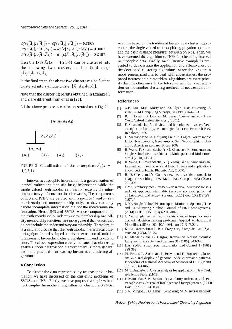
In the final stage, the above two clusters can be further

clustered into a unique cluster {�̃�1, �̃�2, �̃�3, �̃�4}.

Note that the clustering results obtained in Example 1

and 2 are different from ones in [21].

All the above processes can be presented as in Fig. 2.

FIGURE 2: Classification of the enterprises �̃�𝑘(𝑘 =

1,2,3,4)

Interval neutrosophic information is a generalization of interval valued intuitionistic fuzzy information while the

single valued neutrosophic information extends the intui-tionistic fuzzy information. In other words, The components

of IFS and IVIFS are defined with respect to 𝑇 and 𝐹, i.e.,

membership and nonmembership only, so they can only handle incomplete information but not the indetermine in-

formation. Hence INS and SVNS, whose components are the truth membership, indeterminacy-membership and fal-

sity membership functions, are more general than others that

do not include the indeterminacy-membership. Therefore, it is a natural outcome that the neutrosophic hierarchical clus-

tering algorithms developed here is the extension of both the intuitionistic hierarchical clustering algorithm and its extend

form. The above expression clearly indicates that clustering analysis under neutrossophic environment is more general

and more practical than existing hierarchical clustering al-

gorithms.

4 Conclusion

To cluster the data represented by neutrosophic infor-mation, we have discussed on the clustering problems of

SVNSs and INSs. Firstly, we have proposed a single valued

neutrosophic hierarchical algorithm for clustering SVNSs,

which is based on the traditional hierarchical clustering pro-

cedure, the single valued neutrosophic aggregation operator, and the basic distance measures between SVNSs. Then, we

have extented the algorithm to INSs for clustering interval

neutrosophic data. Finally, an illustrative example is pre-sented to demonstrate the application and effectiveness of

the developed clustering algorithms. Since the NSs are a more general platform to deal with uncertainties, the pro-

posed neutrosophic hierarchical algorithms are more prior-

ity than the other ones. In the future we will focus our atten-tion on the another clustering methods of neutrosophic in-

formation.

References

[1] A.K. Jain, M.N. Murty and P.J. Flynn, Data clustering: A

view. ACM Computing Surveys, 31 (1999) 264–323.

[2] B. S. Everitt, S. Landau, M. Leese. Cluster analysis. New

York: Oxford University Press, (2001).

[3] F. Smarandache, A unifying field in logic neutrosophy: Neu-

trosophic probability, set and logic, American Research Pres,

Rehoboth, 1999.

[4] F. Smarandache, A Unifying Field in Logics Neutrosophic

Logic. Neutrosophy, Neutrosophic Set, Neutrosophic Proba-

bility, American Research Press, 2003.

[5] H. Wang, F. Smarandache, Y. Q. Zhang and R. Sunderraman,

Single valued neutrosophic sets, Multispace and Multistruc-

ture 4 (2010) 410-413.

[6] H. Wang, F. Smarandache, Y.Q. Zhang, and R. Sunderraman,

Interval neutrosophic sets and logic: Theory and applications

in computing, Hexis, Phoenix, AZ, (2005).

[7] H. D. Cheng and Y. Guo, A new neutrosophic approach to

image thresholding. New Math. Nat. Comput. 4(3) (2008)

291-308.

[8] J. Ye, Similarity measures between interval neutrosophic sets

and their applications in multicriteria decisionmaking, Journal

of Intelligent and Fuzzy Systems (2013) doi: 10.3233/IFS-

120724.

[9] J. Ye, Single-Valued Neutrosophic Minimum Spanning Tree

and Its Clustering Method, Journal of Intelligent Systems,

(2014) DOI: 10.1515/jisys-2013-0075.

[10] J. Ye, Single valued neutrosophic cross-entropy for mul-

ticriteria decision making problems, Applied Mathematical

Modelling (2013), DOI:10.1016/j.apm.2013.07.020.

[11] K. Atanassov, Intuitionistic fuzzy sets, Fuzzy Sets and Sys-

tems 20 (1986), 87-96.

[12] K. Atanassov and G. Gargov, Interval valued intuitionistic

fuzzy sets, Fuzzy Sets and Systems 31 (1989), 343-349.

[13] L.A. Zadeh, Fuzzy Sets, Information and Control 8 (1965)

338-353.

[14] M. Eissen, P. Spellman, P. Brown and D. Botstein, Cluster

analysis and display of genome- wide expression patterns.

Proceeding of National Academy of Sciences of USA, (1998)

95: 14863–14868.

[15] M. R. Anderberg, Cluster analysis for applications. New York:

Academic Press, (1972).

[16] P. Majumdar, S. K. Samant, On similarity and entropy of neu-

trosophic sets, Journal of Intelligent and fuzzy Systems, (2013)

Doi:10.3233/IFS-130810.

[17] S.A. Mingoti, J.O. Lima, Comparing SOM neural network

{A1} {A4} {A3} {A2}

{A1,A3,A4}

}

{A1,A2,A3,A4}

}

{A1,A4}

}

Neutrosophic Sets and Systems, Vol. 2, 2014

Rıdvan Şahin, Neutrosophic Hierarchical Clustering Algoritms

with fuzzy c-means k-means and traditional hierarchical clus-

tering algorithms. European Journal of Operational Research,

(2006) 174: 1742–1759.

[18] Y. Guo and H. D. Cheng, New neutrosophic approach to im-

age segmentation. Pattern Recognition, 42 (2009) 587-595.

[19] Y. H. Dong, Y. T. Zhuang, K. Chen and X. Y. Tai (2006). A

hierarchical clustering algorithm based on fuzzy graph con-

nectedness. Fuzzy Sets and Systems, 157, 1760–1774.

[20] Z. Hongyu, J. Qiang Wang, and X. Chen, Interval Neutro-

sophic Sets and its Application in Multi-criteria Decision

Making Problems, The Scientific World Journal, to appear

(2013).

[21] Z. M. Wang, Yeng Chai Soh, Qing Song, Kang Sim, Adaptive

spatial information-theoretic clustering for image segmenta-

tion, Pattern Recognition, 42 (2009) 2029-2044.

[22] Z. S. Xu, Intuitionistic fuzzy hierarchical clustering algo-

rithms, Journal of Systems Engineering and Electronics 20

(2009) 90–97.

Received: January 13th, 2014. Accepted: February 3th, 2014