


Languages
Pages
Legal


Network Reliability and
Resiliency in Next
Generation Networks at
Physical, Datalink, and
Network Layers
by
Alex Koudrin
A thesis
submitted to Victoria University of Wellington
in fulfilment of the
requirements for the degree of
Master of Science
in Computer Science.
Victoria University of Wellington
2007


Abstract
The “Next Generation Network”(NGN) will replace today’s separate net-
works for telephone and data. It is expected that the NGN will allow
the introduction of new services, such as broadcast media transmission
and video on demand. A major consideration with the NGN is that it
provides an equivalent voice service quality and resiliency as the cur-
rent telephone network. The analysis carried out for this thesis looked at
the physical reliability of the network topology, network resiliency of the
most popular candidate protocols at datalink and network layers, and
the end-to-end voice performance over an NGN corresponding to the
New Zealand network. This showed that the physical layer reliability of
the network could surpass the reliability of the telephone network. The
results also showed that in a representative ladder-based core network
Multi Protocol Label Switching has a much better resiliency than Open
Shortest Path First. In a representative tree-based access topology MPLS
was found to be superior to Ethernet. The analysis of an end-to-end voice
solution over the NGN yielded results which showed that the network
complies with the most strict standards and the voice is of current tele-
phone quality provided that packet losses in the NGN are below 1.34 %,
which is relatively high to the expected NGN packet loss figures.


Acknowledgments
I would like to thank my supervisor Peter Komisarczuk for his feedback,
patience, and support in helping me produce this thesis.
iii


Contents
1 Introduction 1
1.1 Context and Motivation . . . . . . . . . . . . . . . . . . . . 1
1.2 Research Question . . . . . . . . . . . . . . . . . . . . . . . 4
1.3 Contributions . . . . . . . . . . . . . . . . . . . . . . . . . . 4
1.4 Overview of Main results . . . . . . . . . . . . . . . . . . . 5
1.5 Thesis Outline . . . . . . . . . . . . . . . . . . . . . . . . . . 6
2 Related Work 9
2.1 Public Switched Telephone Network . . . . . . . . . . . . . 10
2.2 Next Generation Network Architecture . . . . . . . . . . . 12
2.2.1 Packet Network Architecture . . . . . . . . . . . . . 14
2.2.2 Migration Path . . . . . . . . . . . . . . . . . . . . . 15
2.2.3 Security . . . . . . . . . . . . . . . . . . . . . . . . . 16
2.3 Last Mile Access Technologies . . . . . . . . . . . . . . . . . 17
2.3.1 Digital Subscriber Line . . . . . . . . . . . . . . . . . 18
2.3.2 Cable . . . . . . . . . . . . . . . . . . . . . . . . . . . 18
2.3.3 Passive Optical Network . . . . . . . . . . . . . . . . 19
2.4 Failure Modes . . . . . . . . . . . . . . . . . . . . . . . . . . 19
2.5 VoIP Transport Concerns . . . . . . . . . . . . . . . . . . . . 20
2.5.1 QoS Concerns of PSTN and VoIP Calls . . . . . . . . 21
v

vi CONTENTS
2.6 VoIP Quality Assessment . . . . . . . . . . . . . . . . . . . . 24
2.6.1 E-model . . . . . . . . . . . . . . . . . . . . . . . . . 24
2.6.2 Objective . . . . . . . . . . . . . . . . . . . . . . . . . 26
2.7 Reliability . . . . . . . . . . . . . . . . . . . . . . . . . . . . 28
2.7.1 Physical Network Reliability . . . . . . . . . . . . . 29
2.7.2 Metrics . . . . . . . . . . . . . . . . . . . . . . . . . . 30
2.8 Resiliency . . . . . . . . . . . . . . . . . . . . . . . . . . . . 31
2.9 Review of Key NGN Protocols . . . . . . . . . . . . . . . . 32
2.9.1 Legacy and Other Protocols . . . . . . . . . . . . . . 32
2.9.2 Open Shortest Path First . . . . . . . . . . . . . . . . 32
2.9.3 Multi Protocol Label Switching . . . . . . . . . . . . 33
2.9.4 Overview of Ethernet . . . . . . . . . . . . . . . . . 35
2.9.5 Rapid Spanning Tree Protocol . . . . . . . . . . . . . 37
2.10 NGN Transport and Signaling Protocols . . . . . . . . . . . 38
2.11 Quality of Service . . . . . . . . . . . . . . . . . . . . . . . . 39
2.11.1 Integrated Services . . . . . . . . . . . . . . . . . . . 40
2.11.2 Differentiated Services . . . . . . . . . . . . . . . . . 40
2.11.3 Other Solutions . . . . . . . . . . . . . . . . . . . . . 41
2.11.4 Metrics . . . . . . . . . . . . . . . . . . . . . . . . . . 42
2.12 Summary . . . . . . . . . . . . . . . . . . . . . . . . . . . . . 44
3 Research Question 45
3.1 Research Question . . . . . . . . . . . . . . . . . . . . . . . 45
3.2 Justification . . . . . . . . . . . . . . . . . . . . . . . . . . . 46
3.2.1 Network Reliability . . . . . . . . . . . . . . . . . . 47
3.2.2 Resiliency . . . . . . . . . . . . . . . . . . . . . . . . 48
3.2.3 Experiment Analysis Steps . . . . . . . . . . . . . . 48

CONTENTS vii
3.2.4 Simulation . . . . . . . . . . . . . . . . . . . . . . . . 49
3.2.5 Failure Modes . . . . . . . . . . . . . . . . . . . . . . 50
3.2.5.1 Other Metrics . . . . . . . . . . . . . . . . . 50
3.2.6 End-to-end Quality Analysis . . . . . . . . . . . . . 51
3.2.6.1 Metrics analysis . . . . . . . . . . . . . . . 51
3.2.6.2 VoIP Analysis with E-model . . . . . . . . 51
3.2.7 Other Issues . . . . . . . . . . . . . . . . . . . . . . . 52
3.3 Core of the Thesis . . . . . . . . . . . . . . . . . . . . . . . . 52
4 Next Generation Core Network 55
4.1 Introduction . . . . . . . . . . . . . . . . . . . . . . . . . . . 55
4.2 Physical Topology . . . . . . . . . . . . . . . . . . . . . . . . 56
4.2.1 Ladder . . . . . . . . . . . . . . . . . . . . . . . . . . 56
4.2.2 Redundant Ladder . . . . . . . . . . . . . . . . . . . 59
4.2.3 Physical Characteristics . . . . . . . . . . . . . . . . 60
4.3 Physical Reliability Analysis . . . . . . . . . . . . . . . . . . 62
4.4 Experiment Setup . . . . . . . . . . . . . . . . . . . . . . . . 65
4.4.1 Performance Metrics . . . . . . . . . . . . . . . . . . 65
4.4.2 Failure Modes . . . . . . . . . . . . . . . . . . . . . . 67
4.4.3 Protocols . . . . . . . . . . . . . . . . . . . . . . . . . 67
4.4.3.1 Overview of OSPF Resiliency . . . . . . . 68
4.4.3.2 Overview of MPLS Resiliency . . . . . . . 72
4.4.4 Simulation Execution and Data Collection . . . . . 74
4.5 Results . . . . . . . . . . . . . . . . . . . . . . . . . . . . . . 76
4.5.1 Uncertainties . . . . . . . . . . . . . . . . . . . . . . 76
4.5.2 Rerouting . . . . . . . . . . . . . . . . . . . . . . . . 78
4.5.3 Packet Loss . . . . . . . . . . . . . . . . . . . . . . . 80

viii CONTENTS
4.5.4 OSPF Hello Timer Variation . . . . . . . . . . . . . . 82
4.5.5 Delay . . . . . . . . . . . . . . . . . . . . . . . . . . . 84
4.5.5.1 Small Link Capacity Study . . . . . . . . . 84
4.5.5.2 Large Link Capacity Study . . . . . . . . . 85
4.5.6 Jitter . . . . . . . . . . . . . . . . . . . . . . . . . . . 86
4.6 Summary . . . . . . . . . . . . . . . . . . . . . . . . . . . . . 87
5 Next Generation Access Network 89
5.1 Introduction . . . . . . . . . . . . . . . . . . . . . . . . . . . 89
5.2 Physical Topology . . . . . . . . . . . . . . . . . . . . . . . . 91
5.2.1 Alternative Topologies . . . . . . . . . . . . . . . . . 94
5.2.2 Physical Characteristics . . . . . . . . . . . . . . . . 94
5.3 Physical Reliability Analysis . . . . . . . . . . . . . . . . . . 95
5.4 Experiment Setup . . . . . . . . . . . . . . . . . . . . . . . . 97
5.4.1 Performance Metrics . . . . . . . . . . . . . . . . . . 97
5.4.2 Failure Modes . . . . . . . . . . . . . . . . . . . . . . 98
5.4.3 Protocols . . . . . . . . . . . . . . . . . . . . . . . . . 99
5.4.3.1 MPLS in the Access Network . . . . . . . 100
5.4.3.2 Ethernet in the Access Network . . . . . . 100
5.4.4 Simulation Execution and Data Collection . . . . . 101
5.5 Results . . . . . . . . . . . . . . . . . . . . . . . . . . . . . . 102
5.5.1 Uncertainties . . . . . . . . . . . . . . . . . . . . . . 102
5.5.2 Rerouting . . . . . . . . . . . . . . . . . . . . . . . . 102
5.5.3 Packet Loss . . . . . . . . . . . . . . . . . . . . . . . 104
5.5.4 Delay . . . . . . . . . . . . . . . . . . . . . . . . . . . 105
5.5.5 Jitter . . . . . . . . . . . . . . . . . . . . . . . . . . . 106
5.6 End-to-end Network Analysis . . . . . . . . . . . . . . . . . 107

CONTENTS ix
5.6.1 Conformance to ITU-T Standards . . . . . . . . . . 108
5.6.2 VoIP Call Quality Analysis . . . . . . . . . . . . . . 110
5.7 Summary . . . . . . . . . . . . . . . . . . . . . . . . . . . . . 112
6 Conclusions 115
6.1 Contributions . . . . . . . . . . . . . . . . . . . . . . . . . . 116
6.2 Future Work . . . . . . . . . . . . . . . . . . . . . . . . . . . 117
A Miscellaneous Core Network Results 127
A.1 Rerouting . . . . . . . . . . . . . . . . . . . . . . . . . . . . . 127
A.1.1 Delay . . . . . . . . . . . . . . . . . . . . . . . . . . . 130
A.1.1.1 Small Link Capacity . . . . . . . . . . . . . 130
A.1.1.2 Large Link Capacity . . . . . . . . . . . . . 132
A.1.2 Jitter . . . . . . . . . . . . . . . . . . . . . . . . . . . 134
A.1.2.1 Small Link Capacity . . . . . . . . . . . . . 134
A.1.2.2 Large Link Capacity . . . . . . . . . . . . . 136
B Miscellaneous Access Network Results 139
B.1 Rerouting . . . . . . . . . . . . . . . . . . . . . . . . . . . . . 139
B.2 Delay . . . . . . . . . . . . . . . . . . . . . . . . . . . . . . . 141
B.3 Jitter . . . . . . . . . . . . . . . . . . . . . . . . . . . . . . . . 142
C Reliability Concepts 143
C.1 Fundamental Concepts . . . . . . . . . . . . . . . . . . . . . 143
C.2 Basic Network Configurations . . . . . . . . . . . . . . . . . 146
C.2.1 Series . . . . . . . . . . . . . . . . . . . . . . . . . . . 146
C.2.2 Parallel . . . . . . . . . . . . . . . . . . . . . . . . . . 146
C.2.3 r-out-of-n . . . . . . . . . . . . . . . . . . . . . . . . 148
C.3 Reliability in Graphs . . . . . . . . . . . . . . . . . . . . . . 149

x CONTENTS
C.3.1 N-modular Redundancy . . . . . . . . . . . . . . . . 149
C.4 Markov Modeling . . . . . . . . . . . . . . . . . . . . . . . . 150
C.5 Fault-Tree Analysis . . . . . . . . . . . . . . . . . . . . . . . 152
C.6 Failure Mode and Effect Analysis . . . . . . . . . . . . . . . 152
C.7 Reliability Optimisation . . . . . . . . . . . . . . . . . . . . 153
C.8 Network Reliability Implementation . . . . . . . . . . . . . 154

List of Figures
1.1 Conceptual comparison of PSTN (top) and NGN (bottom). 2
1.2 Block structure of this thesis . . . . . . . . . . . . . . . . . . 7
2.1 SS7 signaling points and elements . . . . . . . . . . . . . . 11
2.2 NGN functional architecture . . . . . . . . . . . . . . . . . . 13
2.3 End-to-end packet network architecture . . . . . . . . . . . 15
3.1 Network clouds and focus of experiments . . . . . . . . . . 45
4.1 Base ladder topology. Access network and edge router
complexity are simplified. . . . . . . . . . . . . . . . . . . . 57
4.2 Redundant ladder topology . . . . . . . . . . . . . . . . . . 59
4.3 Traffic received by a destination from one source versus
simulation time. Illustration of measurements for a sample
failure. . . . . . . . . . . . . . . . . . . . . . . . . . . . . . . 75
4.4 ETE Delay versus simulation time. Illustration of measure-
ments. . . . . . . . . . . . . . . . . . . . . . . . . . . . . . . . 76
4.5 OSPF HelloInterval variation . . . . . . . . . . . . . . . . . . 83
5.1 Base tree topology . . . . . . . . . . . . . . . . . . . . . . . . 91
5.2 Redundant tree topology . . . . . . . . . . . . . . . . . . . . 93
xi

xii LIST OF FIGURES
5.3 Traffic received by N 0 from all sources, N 0 – N 8 versus
simulation time. Illustration of measurements for a sample
failure. . . . . . . . . . . . . . . . . . . . . . . . . . . . . . . 102
5.4 Summary of the worst case delays in a VoIP path in mil-
liseconds . . . . . . . . . . . . . . . . . . . . . . . . . . . . . 108
5.5 E-model R-value versus error rate e . . . . . . . . . . . . . 111
5.6 E-model R-value versus mouth-to-ear delay . . . . . . . . . 112
C.1 Series configuration . . . . . . . . . . . . . . . . . . . . . . . 146
C.2 Parallel configuration . . . . . . . . . . . . . . . . . . . . . . 148
C.3 Triple modular redundancy configuration with a non-redundant
voter . . . . . . . . . . . . . . . . . . . . . . . . . . . . . . . 150
C.4 Markov reliability model for two identical parallel elements 150
C.5 Inclusion-Exclusion Principle implementation . . . . . . . 155

List of Tables
2.1 Categorisation of Unplanned Failures . . . . . . . . . . . . 20
2.2 Mapping between E-model R-value, MOS, and transmis-
sion speech quality . . . . . . . . . . . . . . . . . . . . . . . 26
2.3 IP QoS class definitions from ITU-T Recommendation Y.1541 [5] 42
2.4 Recommended ETE mouth-to-ear delay for VoIP [1] . . . . 43
4.1 Effective reliability using two parallel paths, P1 and P2, be-
tween E 0 and E 4, given router and link reliabilities . . . . 63
4.2 The ETE reliability, given the reliability of the access net-
work and the core network, ETERel = AccessRel2 · CoreRel 64
4.3 Failure modes examined . . . . . . . . . . . . . . . . . . . . 67
4.4 OSPF configurable timers . . . . . . . . . . . . . . . . . . . 69
4.5 Summary of uncertainties in milliseconds . . . . . . . . . . 77
(a) Small link capacity . . . . . . . . . . . . . . . . . . . . 77
(b) Large link capacity . . . . . . . . . . . . . . . . . . . . 77
4.6 OSPF effective rerouting times in milliseconds . . . . . . . 78
(a) Link failures. Uncertainty range is 145.42 ms. . . . . . 78
(b) Node failures. Uncertainty range is 993.73 ms. . . . . 78
4.7 MPLS effective rerouting times in milliseconds . . . . . . . 79
(a) Link failures. Uncertainty range is 0.41 ms. . . . . . . 79
xiii

xiv LIST OF TABLES
(b) Node failures. Uncertainty range is 0.17 ms. . . . . . 79
4.8 OSPF packet loss to each destination A 0 – A 7 in packets
per second . . . . . . . . . . . . . . . . . . . . . . . . . . . . 81
4.9 Small link capacity. Difference between delay after failure
and delay before failure in milliseconds . . . . . . . . . . . 84
(a) OSPF. Uncertainty range is 0.33 ms. . . . . . . . . . . 84
(b) MPLS. Uncertainty range is 0.13 ms. . . . . . . . . . . 84
4.10 Large link capacity. Difference between delay after failure
and delay before failure in milliseconds . . . . . . . . . . . 86
(a) OSPF. Uncertainty range is 0.56 ms. . . . . . . . . . . 86
(b) MPLS. Uncertainty range is 0.79 ms. . . . . . . . . . . 86
4.11 Small link capacity. Difference between jitter after failure
and jitter before failure in milliseconds. . . . . . . . . . . . 87
(a) OSPF. Uncertainty range before failure is 0.10 ms and
0.09 ms after failure. . . . . . . . . . . . . . . . . . . . 87
(b) MPLS. Uncertainty range before failure is 0.07 ms
and 0.06 ms after failure. . . . . . . . . . . . . . . . . . 87
4.12 Large link capacity. Difference between jitter after failure
and jitter before failure in milliseconds. . . . . . . . . . . . 88
(a) OSPF. Uncertainty range before failure is 0.002 ms
and 0.002 ms after failure. . . . . . . . . . . . . . . . . 88
(b) MPLS. Uncertainty range before failure is 0.001 ms
and 0.001 ms after failure. . . . . . . . . . . . . . . . . 88
5.1 Effective reliability of two parallel paths, P1 and P2, be-
tween S 0 and S 7, given router and link reliabilities . . . . 95
5.2 Failure modes examined . . . . . . . . . . . . . . . . . . . . 98

LIST OF TABLES xv
5.3 Summary of uncertainties in milliseconds . . . . . . . . . . 103
5.4 Ethernet rerouting . . . . . . . . . . . . . . . . . . . . . . . . 103
(a) Link failures. Uncertainty range is 133.05 ms. . . . . . 103
(b) Node failures. Uncertainty range is 180.67 ms. . . . . 103
5.5 MPLS effective rerouting times in milliseconds . . . . . . . 104
(a) Link failures. Uncertainty range is 0.42 ms. . . . . . . 104
(b) Node failures. Uncertainty range is 0.21 ms. . . . . . 104
5.6 Ethernet packet loss from source N 1 – N 8 to destination
N 0 in pps. Without losses N 0 receives 800 pps. Uncer-
tainty range is 0. . . . . . . . . . . . . . . . . . . . . . . . . . 104
5.7 Difference between delay after failure and delay before fail-
ure in milliseconds . . . . . . . . . . . . . . . . . . . . . . . 106
(a) Ethernet. Uncertainty range is 0.45 ms. . . . . . . . . 106
(b) MPLS. Uncertainty range is 0.11 ms. . . . . . . . . . . 106
5.8 Difference between jitter after failure and jitter before fail-
ure in milliseconds . . . . . . . . . . . . . . . . . . . . . . . 107
(a) Ethernet. Uncertainty range is 0.09 ms. . . . . . . . . 107
(b) MPLS. Uncertainty range is 0.05 ms. . . . . . . . . . . 107
A.1 Uncertainty range for OSPF rerouting times in milliseconds 127
(a) Link failures . . . . . . . . . . . . . . . . . . . . . . . . 127
(b) Node failures . . . . . . . . . . . . . . . . . . . . . . . 127
A.2 Uncertainty range for MPLS effective rerouting . . . . . . . 128
(a) Link failures . . . . . . . . . . . . . . . . . . . . . . . . 128
(b) Node failures . . . . . . . . . . . . . . . . . . . . . . . 128
A.3 MPLS average setup and rerouting times . . . . . . . . . . 129
(a) Setup . . . . . . . . . . . . . . . . . . . . . . . . . . . . 129

xvi LIST OF TABLES
(b) Rerouting . . . . . . . . . . . . . . . . . . . . . . . . . 129
A.4 OSPF HelloInterval variation . . . . . . . . . . . . . . . . . . 129
A.5 Small link capacity. Uncertainty range for delay before fail-
ure in milliseconds . . . . . . . . . . . . . . . . . . . . . . . 130
(a) OSPF . . . . . . . . . . . . . . . . . . . . . . . . . . . . 130
(b) MPLS . . . . . . . . . . . . . . . . . . . . . . . . . . . . 130
A.6 Small link capacity. Summary of uncertainty ranges for
delay after failure in milliseconds. . . . . . . . . . . . . . . 131
(a) OSPF . . . . . . . . . . . . . . . . . . . . . . . . . . . . 131
(b) MPLS . . . . . . . . . . . . . . . . . . . . . . . . . . . . 131
A.7 Small link capacity. Delay after failure in milliseconds . . . 131
(a) OSPF. Uncertainty range is 0.38 ms. . . . . . . . . . . 131
(b) MPLS. Uncertainty range is 0.17 ms. . . . . . . . . . . 131
A.8 Large link capacity. Uncertainty range for delay before
failure in milliseconds . . . . . . . . . . . . . . . . . . . . . 132
(a) OSPF . . . . . . . . . . . . . . . . . . . . . . . . . . . . 132
(b) MPLS . . . . . . . . . . . . . . . . . . . . . . . . . . . . 132
A.9 Large link capacity. Uncertainty range for delay after fail-
ure in milliseconds. . . . . . . . . . . . . . . . . . . . . . . . 132
(a) OSPF . . . . . . . . . . . . . . . . . . . . . . . . . . . . 132
(b) MPLS . . . . . . . . . . . . . . . . . . . . . . . . . . . . 132
A.10 Large link capacity. Delay after failure in milliseconds. . . 133
(a) OSPF. Uncertainty range is 0.77 ms. . . . . . . . . . . 133
(b) MPLS. Uncertainty range is 0.83 ms. . . . . . . . . . . 133
A.11 Small link capacity. Uncertainty range for jitter before fail-
ure in milliseconds . . . . . . . . . . . . . . . . . . . . . . . 134
(a) OSPF . . . . . . . . . . . . . . . . . . . . . . . . . . . . 134

LIST OF TABLES xvii
(b) MPLS . . . . . . . . . . . . . . . . . . . . . . . . . . . . 134
A.12 Small link capacity. Uncertainty range for jitter after failure
in milliseconds. . . . . . . . . . . . . . . . . . . . . . . . . . 134
(a) OSPF . . . . . . . . . . . . . . . . . . . . . . . . . . . . 134
(b) MPLS . . . . . . . . . . . . . . . . . . . . . . . . . . . . 134
A.13 Small link capacity. Jitter after failure in milliseconds. . . . 135
(a) OSPF. Uncertainty range is 0.09 ms. . . . . . . . . . . 135
(b) MPLS. Uncertainty range is 0.06 ms. . . . . . . . . . . 135
A.14 Large link capacity. Uncertainty range for jitter before fail-
ure in milliseconds . . . . . . . . . . . . . . . . . . . . . . . 136
(a) OSPF . . . . . . . . . . . . . . . . . . . . . . . . . . . . 136
(b) MPLS . . . . . . . . . . . . . . . . . . . . . . . . . . . . 136
A.15 Large link capacity. Uncertainty range for jitter after fail-
ure in milliseconds. . . . . . . . . . . . . . . . . . . . . . . . 136
(a) OSPF . . . . . . . . . . . . . . . . . . . . . . . . . . . . 136
(b) MPLS . . . . . . . . . . . . . . . . . . . . . . . . . . . . 136
A.16 Large link capacity. Jitter after failure in milliseconds. . . . 137
(a) OSPF. Uncertainty range is 0.002 ms. . . . . . . . . . . 137
(b) MPLS. Uncertainty range is 0.001 ms. . . . . . . . . . 137
B.1 Uncertainty range for RSTP rerouting times in milliseconds 139
(a) Link failures . . . . . . . . . . . . . . . . . . . . . . . . 139
(b) Node failures . . . . . . . . . . . . . . . . . . . . . . . 139
B.2 Uncertainty range for MPLS effective rerouting . . . . . . . 140
(a) Link failures . . . . . . . . . . . . . . . . . . . . . . . . 140
(b) Node failures . . . . . . . . . . . . . . . . . . . . . . . 140
B.3 MPLS average setup and rerouting times . . . . . . . . . . 140

xviii LIST OF TABLES
(a) Setup . . . . . . . . . . . . . . . . . . . . . . . . . . . . 140
(b) Rerouting . . . . . . . . . . . . . . . . . . . . . . . . . 140
B.4 Delay after failure in milliseconds . . . . . . . . . . . . . . . 141
(a) RSTP. Uncertainty range is 0.38 ms. . . . . . . . . . . 141
(b) MPLS. Uncertainty range is 0.13 ms. . . . . . . . . . . 141
B.5 Summary of uncertainty ranges for delay after failure in
milliseconds . . . . . . . . . . . . . . . . . . . . . . . . . . . 141
(a) RSTP . . . . . . . . . . . . . . . . . . . . . . . . . . . . 141
(b) MPLS . . . . . . . . . . . . . . . . . . . . . . . . . . . . 141
B.6 Summary of uncertainty ranges for jitter after failure in
milliseconds . . . . . . . . . . . . . . . . . . . . . . . . . . . 142
(a) RSTP . . . . . . . . . . . . . . . . . . . . . . . . . . . . 142
(b) MPLS . . . . . . . . . . . . . . . . . . . . . . . . . . . . 142
B.7 Jitter after failure in milliseconds . . . . . . . . . . . . . . . 142
(a) RSTP. Uncertainty range is 0.38 ms. . . . . . . . . . . 142
(b) MPLS. Uncertainty range is 0.13 ms. . . . . . . . . . . 142

Chapter 1
Introduction
1.1 Context and Motivation
Next Generation Network (NGN) is a broad concept of a converged net-
work that would carry all services currently supplied by separate net-
works. Considering current residential services we would see best ef-
fort data and voice becoming the two primary services in the near fu-
ture. Future services of the NGN include TV broadcast and high qual-
ity interactive data and voice services, called “triple play”. Voice traffic
is currently transported using the Public Switched Telephone Network
(PSTN), which has a dedicated transport and signaling network. Best ef-
fort data is transported using IP forwarding through a separate network,
sometimes, using the same physical transport links as PSTN.
Figure 1.1 shows the conceptual comparison between PSTN and NGN.
In PSTN an endpoint — the telephone, is connected to a local exchange
(LE). LE is then connected to the core time-division multiplex (TDM)
voice transport network, which consists of transit exchanges (TEs). Sig-
naling System 7 (SS7) is a separate dedicated packet network that pro-
1

2 CHAPTER 1 INTRODUCTION
TE
LE LE
Core
SS7 Packet Treansport Network
TDM Voice Transport
Servers
TE
CRER ER
Servers
CoreCR
Figure 1.1: Conceptual comparison of PSTN (top) and NGN (bottom).
vides all signaling in the PSTN. Any additional services are provided by
the servers attached to SS7 called the Intelligent Network (IN).
The second part of Figure 1.1 shows the NGN at the same level of ab-
straction as the PSTN. The local access parallels that of PSTN, but the ac-
cess point aggregates many subscriber lines into a switch, which connects
to an edge router (ER). An ER connects to the core network consisting
of core routers (CRs). The major difference is that NGN accommodates
signaling and transport using a single packet network, which provides
financial and management advantages over the PSTN. Also, call control
is a function of the residential gateway or the user equipment and servers
in the core network. This is compared to a dumb phone with a local ex-
change on the end of a copper local loop. The LE and signaling network
provide the intelligence to manipulate calls.
PSTN is by definition a carrier grade network, which provides highly
available voice services. Historically, PSTN was built to have “five nines”

SECTION 1.1 CONTEXT AND MOTIVATION 3
— 0.99999 element reliability, which translates into the often measured
and quoted 0.9993 end-to-end reliability. For NGN to be a carrier grade
network it must be at least as reliable as PSTN, provide high quality
transmission guarantees, and be easy to manage and operate [41]. Most
of today’s deployed IP networks do not provide a network availability
equivalent to the PSTN.
In the last decade there have been many advances in network tech-
nology [34]. Hardware switching elements are carrying higher than ever
throughputs with high reliability. Market forces such as traffic and sub-
scriber growth, equipment cost reduction, and new technology penetra-
tion, have deep impact on network buildouts. Some Quality of Service
(QoS) can now be provided using such technologies as Multi-protocol
Label Switching (MPLS).
The technology has matured to the point where it can be used to de-
liver NGN and in the last several years ITU-T has produced several stan-
dards addressing various aspects of the NGN. What remains is testing
the technology in typical network configurations against the NGN stan-
dards. Once the network conforms to the standards it becomes a carrier
grade solution that can safely replace the PSTN.
Migration from PSTN to NGN is happening throughout the world
and New Zealand Telecom is planning to replace PSTN by NGN over the
next decade. Thus, at this time it is vital to determine the effectiveness of
the NGN technology prior to deployment.

4 CHAPTER 1 INTRODUCTION
1.2 Research Question
This thesis investigates the answer to the following question: How well
can current IP and Ethernet technology fulfill NGN network and service relia-
bility and resiliency requirements?
Many aspects of NGN technology need validation against the stan-
dards, however, the focus is narrowed down to the lower three network
layer technologies. Three aspects of current technology are investigated
in this thesis: physical topology; datalink layer protocols, which are MPLS
and Ethernet; and a representative network layer protocols, which is
Open Shortest Path First (OSPF).
Such an investigation needs to be undertaken prior to the NGN roll-
out to make certain the new network will be at least equivalent to the
PSTN voice network today. Physical topologies for various parts of the
network need to be understood in terms of their reliabilities and whether
reliability meets the set target. In particular, this thesis investigates a rep-
resentative ladder topology for the core network and the tree topology
for the access network. Resiliency of the most used protocols — OSPF,
MPLS, and Ethernet — should be compared to select appropriate proto-
cols for NGN deployment. Finally, the end-to-end quality of the voice
service should satisfy the goal of matching or exceeding the PSTN using
the best NGN technology.
1.3 Contributions
This thesis presents three main contributions.
First, is the application of reliability theory to a specific physical NGN
topology, which is chosen to approximate a design for the NGN for New

SECTION 1.4 OVERVIEW OF MAIN RESULTS 5
Zealand. The core and the access network topologies are analysed sepa-
rately and then combined. The analysis demonstrates the range of values
of reliability for the New Zealand NGN and whether those figures con-
form to the NGN requirements.
Second, is the resiliency analysis of the main rival datalink and net-
work layer protocols that are envisaged to be part of NGN. The analysis
involves quality performance assessment by comparing various metrics
to appropriate standards and using models to approximate voice quality.
In the core network OSPF and MPLS are compared, whereas in the access
network Ethernet and MPLS are compared.
Third, is the analysis of the complete end-to-end voice solution, using
the best protocols determined through analysis of the second contribu-
tion.
1.4 Overview of Main results
Both the core and the access network each were found to require 0.9999
reliability to satisfy the end-to-end PSTN reliability of 0.9993. To satisfy
0.9999 reliability, thresholds for individual router and link reliabilities
were calculated. For the core network the router and link reliabilities
must be at least 0.999, whereas for the access network router reliability
must be at least 0.999 and link reliability must be at least 0.9999 or vice
versa.
Resiliency comparison of the datalink and network protocols used
rerouting delay as the primary metric, with packet loss due to rerout-
ing, delay and jitter used as secondary metrics. In the core network OSPF
and MPLS were compared. MPLS was found a much better choice than

6 CHAPTER 1 INTRODUCTION
OSPF because the rerouting delay was at most 13 ms — much smaller
than 6 – 40 seconds for OSPF, which was also supported by the packet
loss endured during the rerouting. The difference between end-to-end
delay after failure and delay before failure was approximately 1.5 ms,
which is around 6 % of the delay before failure. In the access network
Ethernet and MPLS were compared. Again, MPLS dominated the per-
formance with 10 ms rerouting time versus 4 s for Ethernet when using
the Rapid Spanning Tree Protocol to recover from failures. The difference
between end-to-end delay after failure and delay before failure was ap-
proximately 1 ms, which is around 13 % of the delay before failure. The
percentage is larger than that of the core network due to shorter propa-
gation delay. In both cases jitter was seen to be insignificant within the
end-to-end quality of service measurement.
The core and the access results were combined and the complete end-
to-end network was analysed for the quality of voice delivered to users.
Typical values for other parameters were used where the investigation
was out of the scope. According to ITU-T recommendation the end-to-
end solution conformed to the most strict requirements for VoIP service.
The E-model also showed that voice quality is on the par with that of
PSTN even during failures, provided that random packet loss remains
below 1.34 %.
1.5 Thesis Outline
Figure 1.2 shows the overall structure of my thesis. Chapter 2 overviews
the broad scope of related work on NGN. Chapter 3 develops the research
question in some detail. The chapter also narrows down and analyses

SECTION 1.5 THESIS OUTLINE 7
Conclusions
Network
CoreNetwork
RelatedWork
Introduction
ResearchQuestion
Main Contributions
Access
Figure 1.2: Block structure of this thesis
the information presented in Chapter 2 so it is directly relevant to the re-
search question. Chapter 4 analyses reliability of the ladder topology rep-
resenting the core network. It also compares resiliency and quality per-
formance of OSPF and MPLS. Chapter 5 parallels Chapter 4 by analysing
the physical reliability of a tree-based access topology and by comparing
Ethernet and MPLS. At the end, the chapter combines the core and ac-
cess results and analyses the end-to-end voice performance of the NGN.
Chapter 6 draws conclusions, summarises the main contributions, and
provides directions for future work.
Appendix A and B present more extensive results, including uncer-
tainties, for the core network and the access network measurements re-
spectively. Reliability concepts used for computations are described in
Appendix C.


Chapter 2
Related Work
This chapter presents a broad review of literature available on NGN,
which is narrowed down and analysed for the focus of this thesis in
Chapter 3.
To establish the basis to which to compare the NGN, the chapter be-
gins with a brief description of the current telephone network. The archi-
tecture of the NGN is discussed in Section 2.2, which also discusses the
general packet network topology, migration path from PSTN to NGN,
and security issues. Section 2.3 provides a brief overview of the last mile
access technologies, including digital subscriber line and cable. The typi-
cal failure modes in a packet network are discussed in Section 2.4, which
are used to decide what failures to introduce in the experimental work.
Section 2.5 discusses the voice over internet protocol (VoIP) issues,
such as the technical factors that affect voice and general quality of ser-
vice issues of a PSTN and VoIP call. To be able to assess the quality of
a VoIP call Section 2.6 overviews the E-model, objective modeling, and
combinations of the two approaches. Section 2.7 overviews reliability is-
sues in more detail and discusses physical network reliability. The section
9

10 CHAPTER 2 RELATED WORK
concludes by describing end-to-end downtime and defects per million as
the two major metrics to measure physical network reliability.
Making the network reliable at the physical layer means failures still
occur and additional failures may be introduced by higher layers in the
protocol stack. The ability to react to a failure is called network resiliency,
which is described in Section 2.8. Resiliency in this thesis refers to how a
datalink or a network protocol reacts to failure. Section 2.9 overviews the
protocols — OSPF, MPLS, Ethernet with RSTP — that are viewed by the
NGN community as key for the new network. These protocols are used
in the experimental work in this thesis.
Because the NGN combines transport and signaling, there is a set of
signaling protocols identified in Section 2.10. However, these are of much
less importance that transport protocols as they occupy a small fraction of
the total transport bandwidth. Quality of service (QoS) is important for
providing VoIP and there are some common methods for implementing
it, such as differentiated and integrated service architectures. Section 2.11
gives a brief overview of QoS methods and more importantly of metrics
that can be used to determine QoS level of a carrier grade service such as
VoIP.
2.1 Public Switched Telephone Network
There are many books and other resources on Public Switched Telephone
Network (PSTN). The majority of the material in this section is found in
Davidson and Peters [31] and Modarressi and Mohan [58].
PSTN is based on time-division multiplexing (TDM) voice transport.
The control is delegated to a physically separate signaling network, Sig-
SECTION 2.1 PUBLIC SWITCHED TELEPHONE NETWORK 11
TDM Voice Transport
SCPSCP
STP STP
STPSTP
Tru
nk
Cal
lP
roce
ssin
g
Line
Signaling
Central Office Circuit Switch
Central Office Circuit Switch
Cal
lP
roce
ssin
g
Signaling
Tru
nk
Line
SS7 Treansport Network(STPs)
Service Network(SCPs)
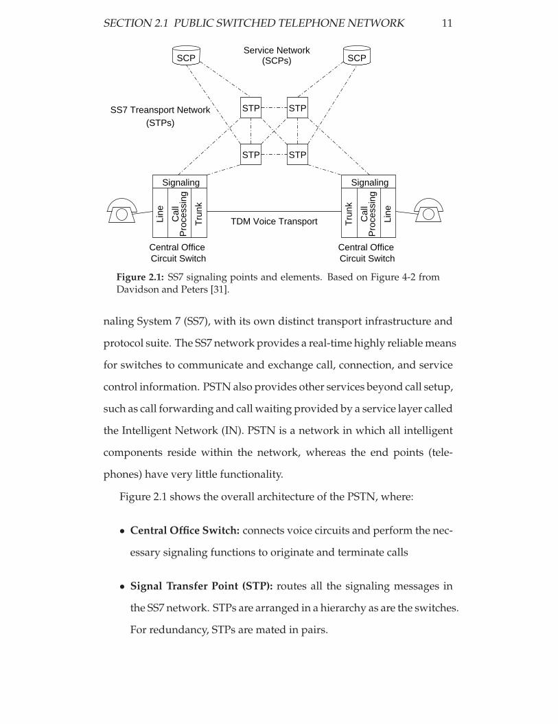
Figure 2.1: SS7 signaling points and elements. Based on Figure 4-2 fromDavidson and Peters [31].
naling System 7 (SS7), with its own distinct transport infrastructure and
protocol suite. The SS7 network provides a real-time highly reliable means
for switches to communicate and exchange call, connection, and service
control information. PSTN also provides other services beyond call setup,
such as call forwarding and call waiting provided by a service layer called
the Intelligent Network (IN). PSTN is a network in which all intelligent
components reside within the network, whereas the end points (tele-
phones) have very little functionality.
Figure 2.1 shows the overall architecture of the PSTN, where:
• Central Office Switch: connects voice circuits and perform the nec-
essary signaling functions to originate and terminate calls
• Signal Transfer Point (STP): routes all the signaling messages in
the SS7 network. STPs are arranged in a hierarchy as are the switches.
For redundancy, STPs are mated in pairs.

12 CHAPTER 2 RELATED WORK
• Service Control Point (SCP): provides access to databases for addi-
tional routing information used in call processing. A SCP is the key
element for delivering IN applications on the telephony network.
Using Figure 2.1 a simplified call setup that involves two local central
office (CO) switches can be analysed. The line module on the incoming
side is responsible for detecting the off-hook event of the connected tele-
phone. The line module then provides dial tone and collects dialed digits.
The processing module analyses the digits passed to it from the line mod-
ule and initiates signaling over the SS7 network. The SS7 network routes
the call setup message to the CO switch of the called party and initiates
the establishment of the voice channel between the two parties over the
TDM network.
2.2 Next Generation Network Architecture
The Next Generation Network (NGN) is a packet based network, which
unifies voice, data, and other potential multimedia services that currently
run over dedicated networks.
There are many organisations and forums that are involved in NGN
development and producing numerous general NGN references, includ-
ing the primary organisation ITU-T [7, 8, 48, 24, 26, 51] ATM Forum [25],
and the Multiservice Switching Forum [33, 30]. There are also several
comprehensive books [28, 57, 62] describe NGN background, issues, and
detailed protocols. Numerous papers, for example, Lee et al. [58, 52] have
also been written on the general NGN architecture and issues.
Figure 2.2 identifies the NGN architecture functional components. The

SECTION 2.2 NEXT GENERATION NETWORK ARCHITECTURE 13
Softswitch
IP Core Network
ApplicationServers
MediaServer
SS7
SignalingGateway
CustomerNetwork
PSTNSwitch
MediaGateway
AccessGateway
AccessNetwork
Figure 2.2: NGN functional architecture based on Figure 1 from Johnsonet al. [46]
architecture has the intermediate elements for compatibility with the cur-
rent PSTN. The short description of the functional elements follows:
Access Network provides connectivity between the customer premise
equipment and the core network. Access method can be one of sev-
eral including broadband and dial-up.
Access Gateway is located in the service provider’s network. It supports
the line interface to the core network for phones, PBXs, and devices.
Functions such as packetisation and echo control are part of access
gateway.
Media Gateway supports a trunk (voice) side interface between to the
PSTN or IP router flows in the packet network. It compresses and
packetises the voice data, and delivers compressed voice packets to
the IP network and vice versa.
Softswitch (also called media gateway controller) handles the registra-
tion and management of resources at the media gateway and is

14 CHAPTER 2 RELATED WORK
responsible for configuration and termination of calls, monitoring
network resources, tracking billing, handling security and authen-
tication, and performing a number of other critical administrative
tasks.
Signaling Gateway provides a signaling interface between VoIP signal-
ing and SS7 signaling.
IP Core Network serves as a high performance transport for IP packet
transport
Media Server is under control of a call agent and provides announce-
ments, tones, and collects user information
Application Server provides additional features not directly hosted on
a call agent
NGN architecture is based around VoIP as its primary service. The
key part of NGN is the softswitch architecture [62], which effectively re-
places the PSTN switching functionality. The three main entities shown
in Figure 2.2 are the signaling gateway interfacing with SS7, media gate-
way interfacing with PSTN voice transport, and the softswitch or the me-
dia gateway controller that provides call control. Section 2.10 identifies
the different protocols used in the softswitch architecture to communi-
cate various functions, such as call control and call state, between the dif-
ferent entities. Ohrtman [62] provides extensive detail on the softswitch
architecture, which is out of scope of this thesis.
2.2.1 Packet Network Architecture
A packet network typically consists of several networks. Figure 2.3 shows

SECTION 2.2 NEXT GENERATION NETWORK ARCHITECTURE 15
End−to−end Connection
AccessAccessNode
Last Mile
CPE
Access AccessNode
Last Mile
CPE
EdgeRouter
EdgeRouter
Core
Figure 2.3: End-to-end packet network architecture
the typical architecture of an end-to-end packet network. It consists of a
low latency and high bandwidth core (or backbone), which typically ex-
tends over a large geographic region such as a country, joined with an
access network by an edge router. The access network aggregates the
traffic from all the access nodes, which perform a lower level aggrega-
tion of individual users connected through a last mile access network.
The last mile may use a variety of technologies, such as ADSL and Cable,
which are briefly described in Section 2.3. Customer Premise Equipment
(CPE) refers to all equipment located past the network interface, such as
router, LAN, and host.
2.2.2 Migration Path
PSTN needs to be replaced by NGN, but it needs to be gradual and seam-
less. Migration from the PSTN to the full NGN is a big issue [28, 57, 25,
10, 61]. As the middle ground PSTN-IP-PSTN architecture is generally re-
garded as the immediate future of NGN. In this architecture the current
PSTN and IP networks are inter-worked together with media gateways

16 CHAPTER 2 RELATED WORK
and signaling gateways as the interfaces. Those gateways are key to reli-
ability and availability of the entire system. For example, if there is only
one gateway then it becomes a single point of failure seriously undermin-
ing end-to-end reliability.
Choi et al. [25] mentions some migration strategies for NGN. Migra-
tion path may involve replacement of class 4 and 5 switches with media
gateways. Alternatively a media gateway may be placed along side of a
switch handling some of the traffic. At the end of the switch lifetime the
traffic can be seamlessly diverted to the media gateway.
2.2.3 Security
PSTN with its separate physical network is very secure [31] due to fac-
tors, such as network intelligence and simple end devices, the nature of
billing makes it almost impossible to affect many network devices. It
is virtually impossible to interfere with a voice conversation. At worst
eavesdropping is possible, which still requires physical access to the line.
IP networks have more security vulnerabilities due to factors such
as, intelligence is at the endpoints instead of the network and the cost
of being connected is much lower than that of PSTN. As a result, NGN
is likely to be susceptible to various security attacks, such as Denial of
Service (DoS), theft of service, and invasion of privacy [33].
There are protective measures against insecurity of data
networks [35]. One extreme option is a completely separate physical net-
work for VoIP. This is currently the most common option to deliver VoIP
capabilities. Virtual overlay networks are also used to achieve a similar
goal. Less drastic measures, in terms of management and financial cost,

SECTION 2.3 LAST MILE ACCESS TECHNOLOGIES 17
include firewalls, intrusion detection, encryption, and authorisation and
authentication techniques.
Increase in security measures also increases the difficulty of NGN op-
eration [33]. For instance, firewalls may make it more difficult to config-
ure VoIP and may degrade its performance, because different and vari-
able ports may be used by the VoIP signaling protocol. Adding more
security means increasing the number of hardware and software compo-
nents in the network, which increases financial costs and decreases net-
work reliability. A significant piece of hardware that is specific to VoIP
security is a Session Border Controller (SBC).
SBCs are typically located between two service provider networks in
a peering environment, or between an access network and a backbone
network to provide service to residential and/or enterprise customers.
They provide a variety of functions to enable or enhance session-based
multi-media services (e.g., VOIP). These functions include: a) perimeter
defense (access control, topology hiding, DoS prevention, and detection);
b) functionality not available in the endpoints (NAT traversal, protocol
interworking or repair); and c) network management (traffic monitoring,
shaping, and QoS). SBCs are envisaged to be a big part of NGN security.
The IETF draft [23] describes more details of the function of SBCs.
2.3 Last Mile Access Technologies
This section gives a brief overview of some of the common last mile ac-
cess technologies. A comprehensive up-to-date reference on last mile ac-
cess technologies is Jayant [45]. Also Black [19] and Tan [79] were used
as supporting references in this section.

18 CHAPTER 2 RELATED WORK
2.3.1 Digital Subscriber Line
xDSL denotes Digital Subscriber Line, where x can be either A(symmetrical),
H(igh-bit-rate), V(ery-high-bit-rate), or S(ymetrical). ADSL is the most
common type of DSL technology used in last mile access. It runs over
the existing PSTN twisted-pair copper cabling. Forward Error Correc-
tion (FEC) is used in ADSL due to PSTN lines being highly susceptible to
noise, such as AM radio. FEC adds up to 20 ms to the end-to-end delay.
The ADSL modem sends and receives data at the customer premises.
An ADSL filter at the customer premise combines voice from a PSTN
phone with ADSL data on the same cable. At the central office exchange
DSL Access Multiplexer (DSLAM) aggregates from 100s to 1000s sub-
scriber lines onto an STM-1 or STM-4 backhaul link.
2.3.2 Cable
Bi-directional Hybrid Fibre-Coaxial (HFC) network is a broadcast tech-
nology created to broadcast video signals to all the endpoints. Data Over
Cable System Interface Specification (DOCSIS) is a set of protocols for
data transmission between a CM and a CMTS. Cable Modem (CM) inter-
faces the user PC on one side and a filter on the other. The filter, combines
video and data channels. The setup parallels that of DSL. Cable Modem
Termination System (CMTS), which is analogous to a DSLAM in ADSL.
A cable network is contended by users in the upstream direction and
broadcast technology is used to transmit downstream. The delay in a ca-
ble network is up to 8 ms, which is much lower than that of ADSL due to
better transmission properties.

SECTION 2.4 FAILURE MODES 19
2.3.3 Passive Optical Network
Passive Optical Network (PON) consists of Optical Link Termination (OLT)
located at the central office exchange; 1:N passive splitter/aggregator lo-
cated near the access region connecting to a maximum of 64 Optical Net-
work Units (ONUs). These entities are linked by fibre connections. For
fibre to the curb deployment, ONUs are located in the road-side cabinets
and users are connect to ONUs using DSL over copper connections.
The main fiber run on a PON network can operate at 155 Mps up to
2.5 Gbps. Downstream data is transported using a broadcast, whereas
upstream data is transported using a time division, multiple access pro-
tocol to avoid collisions at the aggregation point — the splitter.
Ethernet over PON (EPON) is a very promising PON technology. It
combines the ubiquitous low cost and efficient Ethernet technology with
high capacity, low maintenance, up 20 km long reach PON technology.
The delays introduced by any PON is within 1 ms, which is much less
than DSL or cable.
2.4 Failure Modes
Typical failure modes of today’s IP core network have recently been anal-
ysed by Markopoulou et al. [54]. As a result of analysis of Sprint’s IP
backbone network, Markopoulou et al. [54] categorises the failure modes
in Table 2.1, which shows the breakdown of unplanned failures. Planned
maintenance is not shown, because it cannot be avoided in present IP
networks. In NGN maintenance failures may be eliminated as hot swap-
pable IP and MPLS technology improves, which means maintenance can

20 CHAPTER 2 RELATED WORK
Table 2.1: Categorisation of Unplanned Failures. Adapted from Table 3 ofMarkopoulou et al. [54].
be performed without service disruption, except in cases of human error.
My experiments deal with only unplanned failure scenarios.
Markopoulou et al. [54] defines shared and individual sub categories
of unplanned failures. Shared failures are defined as originating from the
same cause. For example, several link attached to a router will share the
same failure if the router processor fails. Individual failures do not share
a cause with any other failures. Such failures are typically link failures.
2.5 VoIP Transport Concerns
Voice over IP (VoIP) is a common term for carrying voice over a packet
network. Much information on packet voice transport is contained in the
general NGN references [7, 8, 48, 24, 26, 51, 25, 33, 30, 28, 57, 62].
The main concern over VoIP is quality [69, 44, 22, 77, 65, 55, 47, 17,
78], which must be maintained at or above the PSTN quality for NGN
to be accepted by consumers. VoIP quality can be influenced in several
different ways.
The coder/decoder (codec) used to encode voice packets greatly in-
fluences voice quality, encoding delay, and bandwidth. Many different
codecs exist, but G.729a is the favorite choice for VoIP in NGN because

SECTION 2.5 VOIP TRANSPORT CONCERNS 21
it satisfies PSTN quality and a good compromise between encoding time
and bandwidth.
End-to-end (ETE) delay is another major factor that affects VoIP qual-
ity. Encoding (and decoding) delay is part of the total delay. There is
also packet assembly, transmission buffer and receiver buffer delays. The
other major source of delay is the general network delay experienced by
all packets flowing between routers and switches to get from source to
destination.
Section 2.6 discusses the E-model and Section 2.11.4 discusses metrics
for packet transport.
2.5.1 QoS Concerns of PSTN and VoIP Calls
This section discusses QoS concerns relating to a typical call in a PSTN
and VoIP networks [39]. The issues include network accessibility, routing
speed, connection setup reliability, routing reliability, connection conti-
nuity, and disconnection continuity. This does not include voice quality,
which is discussed in Section 2.6.
Accessibility is primarily a network issue and is the ability to initiate
a call when desired. It can be measured by the probability that a
user will be unable to use voice services for a given time period.
Accessibility is a critical part of network reliability.
Accessibility of a packet network is similar to accessibility of the
PSTN. However, accessibility may be lower in a hybrid solution
where PSTN and packet network are interfaced together depending
on the reliability of the interface.

22 CHAPTER 2 RELATED WORK
Routing Speed is the rate at which the calls are set up. It can be mea-
sured by a post-dial delay, the time from the last entered piece of
input information to the receipt of the disposition of the request,
such as a ring back or a busy signal.
A packet network is likely to increase the post-dial delay for two
reasons. First, translation between numbers and device addresses
will require a registry look up. Second, negotiation between IP de-
vices is more complex than that of PSTN, for example, Session Ini-
tiation Protocol (SIP) codec negotiation.
Connection Setup Reliability is the probability that a correctly executed
request for a call setup will be extended to the required destination.
If the connection cannot be configured, it is determined as a defect
and clearly contributes to the measure of unreliability of the net-
work.
Additional handling of packets in packet networks is likely to de-
crease connection setup reliability. Hardy [39] hypothesise that the
call completion rate of 99.5 % for the PSTN may drop to 99.0 %,
which is considered barely acceptable.
Routing Reliability is the accuracy of call setup in terms of reaching the
specified destination. As for connection setup the measure is the
misrouted number of call attempts to the total number of calls. This
may be considered as a metric for network reliability as customer
experience is affected by this issue.
This type of reliability is likely to fall due to the additional han-
dling required as in the case of connection setup. There is also an-
other source of potential misroutes originating from the possibility

SECTION 2.5 VOIP TRANSPORT CONCERNS 23
of routing to multiple end-user devices. This is possible when using
the same alias for different IP addresses of devices, such as a desk
phone and a cell phone. If the call is routed to the wrong end device,
this could lead to a misroute from the point of view of the customer.
This aspect of routing reliability is a concern of the service logic.
Connection Continuity is the ability to maintain a connection of a sat-
isfactory quality until call completion. Discontinuities may be the
result of spontaneous disconnects, unacceptable degradation, and
transfer error. A measure for connection continuity is the expected
number of calls that result in disconnects or unacceptable quality
degradation as a function of call duration. The issue is both call ori-
ented and network oriented as both the user is concerned about call
connection and thus reliability of network is affected and measured.
Additional handling of packets in IP networks will increase spon-
taneous disconnects and transfer errors by a marginal amount. The
main concern with packet networks is quality degradation, which
may result users deciding to disconnect voluntarily. The reason for
this is the nature of IP networks where there is no hard reservation
of the call path as in PSTN, where other traffic cannot interfere with
the reserved path. Thus congestion can degrade voice quality in the
middle of a call.
Disconnection Reliability is a measure of whether the disconnection in-
struction produces the desired result, such as correct call termina-
tion and billing. The number of failed disconnection attempts to the
total number of calls is a metric of how good disconnection reliabil-
ity is.

24 CHAPTER 2 RELATED WORK
PSTN has very reliable hardware mechanisms for on-hook and off-
hook events, which therefore can provide accurate billing. In packet
networks a disconnection event is detected using software. There
are also more devices and interactions between them to negotiate
call termination. Thus the additional handling and processing may
decrease the reliability of disconnection and billing by an estimation
of 2 – 4 times that of the PSTN [39].
2.6 VoIP Quality Assessment
To compare VoIP call quality against the traditional PSTN call quality, a
reliable measurement scheme is required. These schemes are outlined in
this section.
2.6.1 E-model
For NGN to constitute an attractive alternative to the traditional PSTN,
it must provide high-quality VoIP services. The problem of assessing
the quality of voice communication over Internet backbones has been
extensively studied in the literature. The most popular model is the E-
model [3] devised by ITU-T, which is used in design of hybrid circuit-
switched and packet-switched networks for carrying high quality voice
applications. The model estimates the relative impairments to voice qual-
ity when comparing different network equipment and network designs.
The E-model estimates the subjective Mean Opinion Score (MOS) rat-
ing of voice quality by using objectively measured quantities over these
planned network environments.

SECTION 2.6 VOIP QUALITY ASSESSMENT 25
In the E-model the terminal, network, and environmental quality fac-
tors are represented by 20 input parameters. A single output of the model
is the R-value (also called the R-factor). Degradation of quality due to in-
dividual quality factors, such as loudness, echo, delay, and distortion,
are calculated on the same psychological scale. Then these are separated
from the reference value. Due to its nature, the E-Model applies only to
telephone band (300 – 3400 Hz) handset communication and it is inappli-
cable to hands-free or wide band communication (150 – 7000 Hz) [3].
Cole and Rosenbluth [27] gives the simplified expression for the R-
factor for various codecs under random packet loss:
R = α − (β1 · d) − β2(d − β3) · H(d − β3) − γ1 − γ2 · ln(1 + γ3 · e),
where: α = 94.2, β1 = 0.024 ms−1, β2 = 0.11 ms−1, β3 = 177.3 ms. For
codec G.729a, γ1 = 11, γ2 = 40, γ3 = 10, whereas for codec G.711 these
values are: γ1 = 0, γ2 = 70, γ3 = 15. The one way mouth-to-ear delay is
given by following relation:
d = dcodec + dde−jitter buffer + dnetwork,
where the total loss probability e is given by:
e = enetwork + (1 − enetwork) · ejitter buffer
Typically ejitter buffer is assumed 0, so e = enetwork. H(x) is a Heavyside
function:
H(x) =
0 if x < 0
1 if x ≥ 0

26 CHAPTER 2 RELATED WORK
Table 2.2: Mapping between E-model R-value, MOS, and transmissionspeech quality
The results for the G.729a codec assume a 20 ms packet size, while the
G.711 results are for a 10 ms packet size. The results for both G.729a
and G.711 listed above are limited to random packet loss. Other values
need to be derived for other combinations of codecs; packet size and error
mask distributions. For the G.729a codec:
R = 83.2 − 0.024d − 0.11(d − 177.3) · H(d − 177.3) − 40ln(1 + 10e)
Table 2.2 shows the R-values corresponding to MOS and speech quality.
R ≥ 80 corresponds to PSTN quality speech.
2.6.2 Objective
Objective modeling is a method to assess the VoIP quality by injecting
sample speech segment across a voice transport path. Using psycho-
acoustic principles, objective modeling compares the output speech with
input speech to produce opinion without reference to underlying channel
conditions. To capture the conversational impairments due to delay, the
low level transport measurements of delay and echo must still be over-
layed on top of this (using the E-model).
Cole and Rosenbluth [27] list the advantages of an objective model as
follows:

SECTION 2.6 VOIP QUALITY ASSESSMENT 27
• No assumptions are made about the underlying network (coder,
de-jitter buffer, error mask, and packet size)
• Results may be more accurate as predicted opinion is based on fun-
damental psycho-acoustics, unlike the E-model, in which an inter-
polation of subjective testing results is used.
Speech layer and packet layer are the two main objective models cur-
rently under standardisation [78].
The disadvantages of objective models are as follows [27]:
• High cost and complexity
• Inaccurate under certain conditions, such as in the case of temporal
clipping
• Intrusive by nature, whereas the E-model can be implemented as
either intrusive or non-intrusive
• The cause of degradation of quality remains unknown
There are efforts to improve the E-model combining it with objective
modeling. For example, Takahashi et al. [78] introduces a second order
polynomial in terms of delay and changes the talker echo impairment
factor. The new model has shown to be a better fit when it was validated
against the data obtained from commercial VoIP products.
Another method [78] directly combines the packet level measurements,
such as delay, jitter, and packet loss. This relies on using thresholds
to define critical quality of voice conversation. Implementation of this
method is very simple, however, defining arbitrarily chosen thresholds

28 CHAPTER 2 RELATED WORK
is it’s weakness, which is overcome by the E-model. Also, it does not at-
tempt to combine the transport metrics in a meaningful way with respect
to voice quality and therefore we ignore it.
2.7 Reliability
PSTN has an ETE reliability of 99.93 % or 0.9993 [28, 46]. The goal of NGN
is to have at least equivalent reliability for the same set of voice services.
Johnson et al. [46] is an excellent summary of VoIP reliability issues.
It lists four techniques required to achieve VoIP reliability:
1. Fault-tolerant hardware is a traditional means of achieving reliabil-
ity by seamlessly switching to a redundant element within a single
platform
2. Fault-tolerant software relies on duplicating software processes
3. Physical network reliability relies on duplicating low reliability net-
work elements to achieve higher network reliability
4. VoIP element interface redundancy employs multiple interfaces and
real-time switch over between them
Out of the four techniques, physical network reliability is explored
further. Reliability of networks is a vast and complex mathematical and
statistical area. This has been a big research in early in 20th century as
electricity grids and PSTN needed to be designed with very high reliabil-
ity. For computer networking only a small part of the field is needed to es-
timate the physical layer reliability. There are many books written about
reliability, a particularly good source is Shooman [74], which has been

SECTION 2.7 RELIABILITY 29
used as an extensive reference to reliability and the underlying statistics
concepts.
2.7.1 Physical Network Reliability
Appendix C defines basic reliability concepts delves into more technical
details of reliability aspects used in my thesis. This section provides a
non-technical overview.
Element reliability at the lowest level is reliability of a single network
element such as an IP router or switch. A router is a device for switch-
ing packets and contains two processors: a route processor and a line
card. Routers are usually designed with redundant processors, line cards,
power supplies and so on. Current router availability is potentially better
than 99.999 % with appropriate redundancy in place. In reality it is closer
to 99.90 % – 99.99 % due to the following factors.
• Chassis remain a single point of failure with large mean time to
repair
• To minimise time to market, development and testing is shortened
• Software and hardware upgrades can cause 10 – 60 min downtime
per year [46]
• Denial of Service (DoS) attacks can cause outages [28, 57]
In 2004, effective router reliability was only 0.9990 to 0.9999 due to main-
tenance downtime, software and chassis low reliability and average link
reliability was approximately the same [82, 46]. Currently, in the year
2006, vendors advertise routers and switches with 0.99999 [6] reliability

30 CHAPTER 2 RELATED WORK
due to hitless switchover technology — eliminating maintenance down-
time, improved software and hardware redundancy.
PSTN element reliability should not be used for all VoIP elements.
VoIP networks vary in size, function, use fault tolerant protocols, and
use more redundant components than PSTN. Thus the reliability require-
ments for a single element should be based on network design and com-
plexity of the element.
2.7.2 Metrics
VoIP service is defined to be available only if the logical end-to-end con-
nection can be completed with sufficient QoS and the calls can be main-
tained for sufficient time to complete the transaction [46].
Johnson et al. [46] proposes two major metrics for reliability: end-to-
end downtime and Defects Per Million (DPM).
End-to-end downtime models a single path between the two end de-
vices such as POTS phones. The path will involve a sequence of equip-
ment such as switches and routers that make the call possible. Each ele-
ment in the sequence has a reliability measurement and combined those
reliabilities produce the total path reliability. This measure does not re-
flect the impact of outages on customers as it does not incorporate cus-
tomer demand during outages. Downtime is usually calculated in min-
utes per year, thus yearly downtime Y D = (1−A)× 525600 min/yr with
A = 99.999 % corresponding to YD = 5.26 min/yr.
DPM counts customer demands not served. More precisely DPM is
the average number of blocked and cutoff calls per million attempted
calls. DPM = (1 − A) × 106. Thus A = 99.999 % corresponds to 10 DPM.

SECTION 2.8 RESILIENCY 31
2.8 Resiliency
Resiliency is the ability to react to a failure, whereas reliability tries to
minimise failures by using redundant network elements.
Failure resiliency is very important in NGN as it ensures the ETE ser-
vice is highly available. Effectively, resiliency makes the reliability vis-
ible at a higher layer of the network protocol stack. For example, with
two two separate physical paths between two points if one of the paths
fails, the a higher layer protocol needs to detect the failure and reroute
the traffic using one of the redundant paths to take advantage of the high
reliability. If on the contrary the protocol had no resiliency, only one re-
dundant path could be used, which effectively decreases the reliability to
a single path.
There has been some research in Europe in the Protection Across Net-
work Layers (PANEL) project, into trying to build models to analyse the
multilayer resilience mechanisms [32]. The models are high level, involv-
ing a lot of approximations. The difficulty is that resiliency depends on
which protocols are used at each layer, how they interact with one an-
other in the face of failure. Improvement in coordination between re-
silience mechanisms is the ultimate goal of the PANEL project. However,
more research efforts are needed to get closer to that goal. The outcome
is a set of guidelines for the type of failure recovery strategy needed in
specific situations. In practice, miscoordination often occurs resulting in
failure detection time being much longer than it could have been. From
time to time network managers typically change protocol configuration
in the network to try and improve failure resiliency.

32 CHAPTER 2 RELATED WORK
2.9 Review of Key NGN Protocols
This section examines the most popular current protocols that are candi-
dates for NGN. The three key protocols are OSPF, MPLS, and Ethernet.
Some of these protocols can be used in the core network and/or the ac-
cess (aggregation) network in Figure 2.3. OSPF is a routing protocol that
is used only in the core network. Ethernet is a datalink protocol used only
in the access network. MPLS is a datalink protocol and it can be used in
both core and access networks.
2.9.1 Legacy and Other Protocols
Other technologies, such as Asynchronous Transfer Mode (ATM) and
Frame Relay (FR), are not examined as they are recognised to be older
technologies that are being gradually phased out of packet networks [57].
These protocols provide performance guarantees, but suffer from many
disadvantages, such as being very complicated and difficult to scale.
Routing protocols such as RIP, ISIS, and BGP are either legacy pro-
tocols, much less popular, or inappropriate. RIP has been surpassed by
OSPF, whereas a very similar Intermediate System to Intermediate Sys-
tem (ISIS) operates in parallel with OSPF but it is used much less in net-
works today. Border Gateway Protocol (BGP) [53] is not are examined as
it provides inter domain connectivity.
2.9.2 Open Shortest Path First
This section overviews OSPF [60] protocol, concentrating on failure re-
covery. A lot of the material is covered in Pasqualini et al. [64].

SECTION 2.9 REVIEW OF KEY NGN PROTOCOLS 33
One of the most common intra-domain routing protocols in IP net-
works is OSPF. The Hello protocol is used for the detection of topology
changes. Each router periodically emits Hello packets on all its outgo-
ing interfaces. If a router has not received Hello packets from an adjacent
router within the RouterDeadInterval, the link between the two routers is
considered down. When a topology change is detected, the information
is broadcasted to neighbours via Link State Advertisements (LSA).
Each router maintains a complete view of the OSPF area, stored as an
LSA Database. Each LSA represents one link of the network, and adjacent
routers exchange bundles of LSAs to synchronise their databases. When
a new LSA is received the database is updated and the information is
broadcasted on outgoing interfaces.
Routes calculation: congurable cost values are associated to each link.
Each router then calculates a complete shortest path tree. Only the next
hop is used for the forwarding process.
The Forwarding Information Base (FIB) of a router determines which
interface has to be used to forward a packet. After each computation of
routes, the FIB must be reconfigured.
Typically a router failure is detected within 30 to 40 seconds, while
a link failure can be detected using hardware detection in under 10 sec-
onds.
2.9.3 Multi Protocol Label Switching
There is a data plane and a control plane to Multi Protocol Label Switch-
ing (MPLS) [66].
The data plane is analogous to ATM virtual paths (VPs) and virtual
circuits (VCs) as MPLS is a connection-oriented by means of Label Switch

34 CHAPTER 2 RELATED WORK
Paths (LSPs). Instead of using ATM VP/VC identifier, MPLS uses 20-bit
labels to identify a connection. This allows up to a theoretical maximum
of 1 million LSPs per interface. This number can be much higher, since
MPLS additionally supports label stacking, which is comparable to the
use of ATM VP/VCs. However, contrary to ATM, label stacking is not
limited to one level, but could be extended to an arbitrary depth.
In core networks, the endpoints and intermediate nodes of the LSP
will typically be IP routers. The endpoints of the LSP are called label
edge routers (LER), whereas the interior nodes are called label switching
routers (LSRs).
MPLS control plane is responsible for establishing an MPLS connec-
tion, which can be done in several ways. The first method is to manually
configure the LSP in each of the involved network elements using a net-
work management tool. This is the equivalent of an ATM PVC and does
not require the use of an MPLS control plane. Another model is to estab-
lish the LSP using MPLS signaling protocols, equivalent to ATM SVCs, or
ATM soft-PVCs. Two commonly used MPLS signaling protocols are the
Label Distribution Protocol (LDP) [12] and Resource Reservation Proto-
col with extensions for LSP establishment, or traffic engineering (RSVP-
TE) [15]. Traffic engineering is about arranging traffic flows around the
network to avoid congestion. RSVP-TE provides mechanisms for doing
that. The control plane is based on network layer protocols and thus uses
IP addressing.
MPLS is the best of both IntServ and DiffServ architectures. As in Diff-
Serv traffic is aggregated into classes (forward equivalence class or FEC),
but there is an unlimited amount of classes or labels in MPLS. A class can
be introduced and all that needs to be done is to circulate the new label

SECTION 2.9 REVIEW OF KEY NGN PROTOCOLS 35
and its level of QoS around the network. The labels are distributed using
a Label Distribution Protocol (LDP).
Unlike DiffServ MPLS is not per hop, but similar to IntServ it sets up
a path, called a label switch path (LSP) for an aggregated flow through
the network. This way MPLS achieves the scalability of DiffServ and the
path set up of IntServ.
MPLS is the most likely to be used to provide QoS. Specifically, pro-
viding voice QoS requires setting up a LSP for voice traffic only once.
All voice traffic will be aggregated into that class and so all packets will
follow the same path through the network.
The main benefits of MPLS are [63]:
• Similar to ATM, MPLS is connection oriented which provides ag-
gregation and segregation of customer traffic
• Scalable technology as label stacking can be performed to arbitrary
depth
• It can tunnel any IP or non-IP protocol
• Inherent support for CoS and QoS
• Many recovery options with performance close to SONET/SDH
2.9.4 Overview of Ethernet
Ethernet is a data link protocol, where the concept of connection is re-
placed by use of a single Ethernet broadcast domain. The network ele-
ments are self learning Ethernet switches that send frames to their final
destination.

36 CHAPTER 2 RELATED WORK
There is no signaling involved, nor is there a need for any higher layer
protocol to be involved, such as a network protocol for label distribution
in MPLS. This is because Ethernet uses the Rapid Spanning Tree Protocol
(RSTP) to eliminate loops and recover in an event of a failure.
Ethernet has traditionally been a LAN technology, however, recently
Meddeb [56] proposed Ethernet for WANs due to various advantages
such as low cost and ease of use of the protocol. However, Ethernet needs
significant alterations for it to become a carrier grade WAN protocol.
Ethernet is rapidly migrating from being a LAN technology to access
network. It was described in an earlier section. The protocol is considered
to be one of the two protocols for access networks.
There are advantages and disadvantages of using Ethernet in the ac-
cess network [56]. The advantages are:
• Granular access speed ranges from 10 Mbps to 10 Gbps
• Efficient multipoint connections support
• No or little training and learning from customers
• No frame termination needed at the CPE
• Low deployment costs due to ubiquitous characteristics of Ethernet
The disadvantages include:
• Contention with proven and widely deployed WAN technologies
• Need for compromise between carrier grade and SLA support ver-
sus simplicity and flexibility of Ethernet
• Interoperability concerns between resilience at other layers and span-
ning tree protocol

SECTION 2.9 REVIEW OF KEY NGN PROTOCOLS 37
• 802.1p frame prioritisation does not necessarily provide end-to-end
QoS
• Potential scalability and latency issues due to large numbers of MAC
addresses
• OAM protocols and tools need to be modified substantially
This thesis investigates resiliency, so for Ethernet, RSTP is the key fo-
cus.
2.9.5 Rapid Spanning Tree Protocol
Unlike routers, switches and bridges do not age-out old packets. This
causes problems such as unicast frame duplication and multicast frame
multiplication. When two or more switches are connected in a loop, they
can multiply multicast frames, sending them round infinitely. The inabil-
ity to tolerate active loops is a fundamental restriction of bridged net-
works.
Redundant connections are essential when designing high-availability
systems, and that is where Rapid Spanning Tree Protocol (RSTP)IEEE
802.1D [9] is used. By blocking redundant connections, RSTP enables a
single/primary data path between nodes, creating a tree topology, which
is a graph with no loops with no disconnected nodes. If a device or a link
failure causes this primary path to become unusable, RSTP will enable a
secondary path. The predecessor of RSTP is STP [9], which has very slow
re-convergence time of 30 to 50 seconds compared to RSTP with several
seconds re-convergence.

38 CHAPTER 2 RELATED WORK
2.10 NGN Transport and Signaling Protocols
There are many types of signaling involved in a VoIP network. It is im-
portant to discuss these protocols because they contribute to the reliabil-
ity metrics discussed in Section 2.7.2. Three categories of signaling are
distinguished, voice transport, transport of SS7 signaling, inter-gateway
signaling within the softswitch model, and service layer signaling.
Voice Transport and Media Signaling Voice packets are carried over IP
using Real Time Protocol (RTP) [71] which uses UDP. Real Time
Control Protocol (RTCP) [72] is used to control the voice packets
. RTCP mainly provides quality related feedback from the receivers
to the transmitter about the state of the RTP flow. Network oper-
ator can use RTCP to monitor quality of voice calls and network
problems.
Stream Control Transmission Protocol The function of Stream Control
Transmission Protocol (SCTP) [76] is to carry SS7 signaling between
a signaling gateway and a softswitch over the NGN. The protocol
is designed to have the speed of UDP and reliability of TCP as pro-
vided by SS7 signaling in PSTN.
MGCP and MEGACO/H.248 Media Gateway Control Protocol (MGCP) [13]
and the more popular MEGACO/H.248 [29] are the two master-
slave protocols used between a softswitch and a media gateway.
H.323 ITU-T Recommendation H.323 [2] describes H.323, which is a sig-
naling protocol for VoIP. The architecture consists of end terminals,
gateways, gatekeepers to control functionality, and multipoint con-
trol units which are used for multi-terminal interaction.

SECTION 2.11 QUALITY OF SERVICE 39
H.323 is a complex protocol suit because it consists of many differ-
ent protocols for doing various functions. Communication involves
many message exchanges, which complicates and retards the speed
of interaction considerably. H.323 is used extensively in todays en-
terprise VoIP in a variety of products and so forms part of NGN.
Session Initiation Protocol Session Initiation Protocol (SIP) [38], is as ex-
pressive a signaling protocol as H.323. SIP has a simpler architec-
ture, message syntax, and it is easily extensible. SIP is based on
a client-server model, in which a client sends SIP requests and a
server responds to SIP requests.
SIP messages are plain text messages with a small number of head-
ers. This makes it simple to communicate, around 5 messages ac-
complish call setup whereas it takes around 20 messages for H.323.
Plain text messages are human readable, making it much easier to
find errors than the Abstract Syntax Notation 1 (ANS.1) notation
used in H.323.
Simplicity and extendibility of SIP make it attractive for VoIP use.
However, it may need extensions to handle security and fault tol-
erance with distributed SIP servers. The extensions are considered
far less formidable than with H.323.
2.11 Quality of Service
Quality of Service (QoS) is a very important aspect that separates NGN
from the current best effort Internet. A particular type of traffic is classi-
fied into a service class (CoS) and is treated according to that classification

40 CHAPTER 2 RELATED WORK
within the network. Prime examples are network management traffic is
usually assigned to the best class and voice traffic is assigned to the sec-
ond highest class. Typically the lower the CoS the worse its performance
in the network, which may include higher end-to-end delay, packet drop,
and so on.
There are three main methodologies for solving the QoS problem.
First is reserving resources on the path to destination prior to the session.
Second is classification of traffic into different classes that are treated with
a different QoS in the network. Third,, bandwidth overprovisioning of
network elements to avoid congestion of all traffic is the simplest but a
more costly solution, since all sections of the network will be underuti-
lized especially during the non-failure operation.
2.11.1 Integrated Services
Integrated Services (IntServ) [21] is a per flow architecture, where each
individual traffic flow reserves resources on its path to the designation to
satisfy required QoS. Resource ReserVation Protocol (RSVP) is used to re-
serve the path resources and admission control. The IntServ architecture
is usually considered too complicated and demanding on the network
and so it is scarcely used by itself.
2.11.2 Differentiated Services
Differentiated Services (DiffServ) [20] uses the concept of aggregating
traffic flows into a set amount of classes. The marking and shaping of
the traffic is achieved by using the DiffServ Code Point IP field. The Diff-
Serv architecture is more scalable than IntServ as only little amount of

SECTION 2.11 QUALITY OF SERVICE 41
state needs to be maintained by the network. The main obstacle to Diff-
Serv is it is on a per hop basis and so a voice packet may take a different
route than the one in the same session thus changing the delay, jitter, and
packet loss. Thus DiffServ is not suitable for sessions that require fixed
QoS, such as VoIP or video conferencing.
A combination of IntServ and DiffServ is also possible, such as IntServ
operation over DiffServ networks, defined in RFC 2998 [18].
2.11.3 Other Solutions
There are many QoS solutions based on QoS and constraint-based rout-
ing. Constraint-based routing is outside of the scope of this thesis, be-
cause it is a large separate field of research.
One interesting example is resilient differentiated QoS (RD-QoS) [14],
which is a combination of DiffServ and routing mechanisms. The ap-
proach argues that resilience to failure of different traffic classes is as im-
portant as QoS classes. Four resilience classes are proposed, with the
first most resilient class having 10 – 100 ms recovery time and a pre-
established recovery path among other specifications. As the classes progress
recovery time increases together with other parameters reflecting lower
resilience needs. RD classes are proposed to be signaled together with
QoS signaling by extending RSVP. The classes are mapped to MPLS re-
covery schemes and they can also be mapped to other QoS architectures
such as DiffServ.

42 CHAPTER 2 RELATED WORK
2.11.4 Metrics
The simple transport level metrics important to assess VoIP quality are
ETE delay, jitter, packet loss, and packet error rate.
ITU-T Recommendation Y.1541 [5], summarised by Seitz [73], speci-
fies numerical values to be achieved for each of the key performance pa-
rameters defined in Y.1540 [4], on international IP network paths. A path
extends from the network interface of the source user to the network in-
terface of the destination user. Customer premise equipment is not part
of the path. The specified values are grouped in a number of distinct
QoS classes to establish a practical basis for communication between end
users and network providers, and among providers, on the quality to be
supported in ETE IP paths.
Table 2.3 specifies Y.1541 performance objectives and QoS classes. Each
QoS class creates a specific combination of bounds on a subset of the per-
formance values. Classes 0 and 1 place upper bounds on packet transfer
delay and packet loss. They also limit packet delay variation. Classes 2
and 3 place upper bounds on packet transfer delay and packet loss, but
do not limit packet delay variation. Classes 0 and 2 differ from classes
1 and 3 in their packet transfer delay objectives. Class 4 limits packet
loss and provides a very soft upper bound on delay. Y.1541 also defines
an unspecified class (class 5) that provides no specific performance guar-
Table 2.3: IP QoS class definitions from ITU-T Recommendation Y.1541 [5]

SECTION 2.11 QUALITY OF SERVICE 43
antees. The value for the single packet error ratio objective was chosen
to ensure that packet loss is the dominant cause of defects presented to
upper layers.
The ETE delay objectives of Class 0 and 2 will not always be achiev-
able on long paths [73]. If only propagation delay is taken into account
the maximum length of a path satisfying the delay of 100 ms is 0.1 s ×
2 × 108 m/s = 2 × 10⁷m = 20, 000 km. Due to node delays this length
is unachievable. However, for New Zealand this is not a problem as the
maximum distance from the bottom of the South Island to the top of the
North Island is less than 2000 km.
Table 2.4 identifies acceptable VoIP mouth-to-ear delays in terms of
user experience, suggested by the ITU-T Recommendation G.114 [1], but
has no relation to the E-model. The delay includes all possible delays
incurred on the path between two users.
Delay will always be present in a VoIP path. The two major classes of
delay are codec related delay and network delay [28, 57]. Codec related
delay is a sum of codec processing, de-jitter buffer, serialisation, packeti-
sation delays. Network delay applies to all packets in the network (pro-
vided they are in the same class of service). The major contributors to
network delay are interface queuing, transmission and node processing
delays [57].
In addition to the formal specifications there are two less formal crite-
ria that a VoIP service may satisfy. One of these an interruption or a fail-
Table 2.4: Recommended ETE mouth-to-ear delay for VoIP [1]

44 CHAPTER 2 RELATED WORK
ure below the network layer should not be longer than 200 ms, in order to
prevent failure detection at the network layer following a timeout. This
time is agreed upon in the network community [28] not only for VoIP but
other real time carrier grade services. The second criteria concerns purely
VoIP because it is a direct consequence of the way the call session is con-
figured and maintained. According to Johnson [46], a VoIP call session is
terminated if any activity between the calling parties is absent for longer
than approximately 2 seconds. This can be regarded as a maximum time
for failure recovery. If a failure cannot be detected and repaired in less
than about 2 seconds all VoIP call sessions currently active (and any new
attempts) will be terminated causing extremely adverse consequences.
2.12 Summary
A broad review of literature has been presented. Reliability, resiliency,
routing protocols, and quality of service that are most significant for my
research have been described in more detail. Chapter 3, analyses these
aspects with respect to the aim of my work.

Chapter 3
Research Question
3.1 Research Question
The question this thesis tries to answer is:
How well can current IP and Ethernet technology fulfil NGN
network and service reliability and resiliency requirements?
The three pieces of current technology investigated are the physical topol-
ogy, datalink layer protocols, and network layer protocols. NGN is in-
vestigated in two sections, the core network and the access network. Fig-
ure 3.1 shows all the major parts of the ETE network topology. The focus
of physical reliability and resiliency experimental work is the core and
access network.
Scope of Experiments
CoreCPE Last Mile Access Access Last Mile CPE
Figure 3.1: Network clouds and focus of experiments
45

46 CHAPTER 3 RESEARCH QUESTION
Physical topology is the basis for other layers in the network protocol
stack. The configuration of network elements and their types and qual-
ity determine physical layer reliability. My thesis investigates physical
reliability of the core and access network separately, because they have
different topologies and requirements. The results of these analyses are
combined to develop an ETE reliability analysis.
Analysis in Chapter 2 shows the important aspects related to answer-
ing the research question. Section 2.7 identified physical network relia-
bility as the most relevant issue and identified two measures in particu-
lar, DPM and end-to-end downtime. Section 2.5.1 showed that the most
important aspect of resiliency is network accessibility. The best metrics
to assess resilience were shown in Section 2.11.4 to be ETE delay, jitter,
packet loss, and packet error rate. The selection of the protocols for the
study is provided in Section 2.9. OSPF and MPLS are selected for com-
parison in the core network and Ethernet and MPLS in the access net-
work. Section 2.11.4 describes the resulting end-to-end network solution
assessment in terms of voice quality. Two ITU-T recommendations and
some less formal measures are used to compare network metrics. The
E-model in Section 2.6.1 is identified to be the best model to assess VoIP
voice quality against that of the PSTN.
3.2 Justification
The focus of this research is determined as physical reliability, protocol
resiliency, and assessing the ETE quality of NGN. These aspects are de-
tailed in the following sections. In this section I determine the justifica-
tion for this specific focus.

SECTION 3.2 JUSTIFICATION 47
3.2.1 Network Reliability
Physical network reliability is selected in Section 2.7 out of a number of
reliability issues, because it constitutes a large part of the reliability space.
Appendix C describes techniques for calculating network reliability.
Using these techniques, the core and access topologies are analysed sep-
arately and combined for a complete reliability measure.
The metric used for reliability is the ETE downtime measure, which is
identified in Section 2.7.2. For theoretical computation of reliability ETE
downtime equivalent to the DPM measure. The two metrics are subtly
different when using real network data because DPM counts user de-
mands not served.
Reliability, which is regarded equivalent to availability in networks, is
primarily a measure of network accessibility (Section 2.5.1), which consti-
tutes the main part of quality concern. The secondary concern is connec-
tion continuity, because it is important that the call progresses without in-
terruptions and is of consistent level of quality throughout the call. Con-
nection continuity is indirectly measured by simulation rerouting time
and other metrics indicating the level of ETE quality. The quality con-
cern is investigated at the end of Chapter 5 as part of the ETE network
analysis. The reliability issues identified in Section 2.5.1, but which are
not part of the scope of this thesis are as follows. Routing speed is a
customer related issue and does not have much bearing on network re-
liability. Connection setup reliability is not directly related to reliability.
Routing Reliability is a concern of the service logic.

48 CHAPTER 3 RESEARCH QUESTION
3.2.2 Resiliency
As Section 2.8 described, resiliency of higher layer protocols is very im-
portant because it effectively translates the physical layer reliability to
higher layer. Examining and comparing resiliency of datalink and net-
work layer protocols is therefore of great importance in answering the
research question.
3.2.3 Experiment Analysis Steps
Hassan and Jain [40] in Chapter 4 describe a methodology for a system-
atic simulation study. The steps are as follows.
1. Define the objective of the study
2. Design reference network model and select fixed parameters
3. Select performance metrics
4. Select variable parameters
5. Construct the network model and set fixed parameters in simula-
tion software
6. Configure simulation software to produce relevant performance data
7. Execute simulation program and collect performance data
8. Present and interpret results
For the purpose of the thesis these steps are modified and combined
with Law and Kelton [50] general advice on performing simulation anal-
ysis.

SECTION 3.2 JUSTIFICATION 49
3.2.4 Simulation
Law and Kelton [50] define Discrete Event Simulation (DES) as:
”Discrete event simulation concerns the modeling of a system
as it evolves over time by a representation in which the state
variables change only at a countable number of points in time.
These points in time are the ones at which an event occurs,
where an event is defined to be an instantaneous occurrence
which may change the state of a system.”
DES is a method used to model real world systems able to be decom-
posed into a set of logically separate processes autonomously progress-
ing through time. Each event must take place on a specific process, and
must be assigned a logical time (a timestamp). The result of this event
can be a message passed to one or more other processes (including, if re-
quired, the process on which the event occurred). On arrival at this other
process, the content of the message may result in the generation of new
events, to be processed at some specified future logical time.
The principle restriction placed on DES is that an event cannot affect
the outcome of a prior event, that is, logical time cannot run backwards.
DES is used because this is the only accurate method to investigate
the performance of a network in response to a failure. An alternative ap-
proach to DES is analytical modeling, which cannot accurately predict
the outcome when there is a complex mix of traffic from multiple traffic
sources and and failure consequences need to be analysed. Such models
are only useful for calculating steady state of a network, when all pro-
cesses have settled down.

50 CHAPTER 3 RESEARCH QUESTION
For all my simulations I used Opnet, because it is one of the best DES
simulators and it contains models of the majority of the NGN technology
required. The other major alternative network simulator is NS 2, which
was ruled out because it needed several non-trivial extensions to perform
the required simulations.
3.2.5 Failure Modes
From Table 2.1 we see that more than two thirds of unplanned failures are
individual link failures, whereas router-related failures contributes only
16.5 %. My thesis discards the optical and unspecified shared failures,
because the optical layer is part of the physical layer, which is not inves-
tigated. Unspecified failures are difficult to simulate because their cause
is not determined or classified.
According to Table 2.1, simultaneous failures of core routers is suffi-
ciently low. The probability of a simultaneous failure of two independent
routers is the probability of one router failure times the unavailability all
squared. According to Miller [57], typical router availability is between
99.99 and 99.9999 %. Unavailability = 1 – Availability, so the worst un-
availability for a router is 0.01 %. Using the figure of single router failure
probability of 16.5 % from Table 2.1, simultaneous router failure is (16.5 %
x 0.01 %)2= 0.00027 %, provided router failures are independent events.
Such an event is extremely negligible and therefore not examined.
3.2.5.1 Other Metrics
The main network metrics used for measurement and identified in Sec-
tion 2.11.4 are ETE, because these are the most meaningful in all models
and standards. The ETE metrics depend on delay, jitter, packet loss, and

SECTION 3.2 JUSTIFICATION 51
packet error rate measurements. ETE delay is the most significant of the
metrics in terms of influence on quality performance. Packet loss as a
result of the network reconfiguration is a significant measure of protocol
resiliency. Random packet loss is not simulated explicitly, but it is used
in the E-model calculations to indicate the range of values of packet loss
that can be tolerated.
Per network element metrics are not very useful for my experiments.
These are processing delays, propagation delays, and queuing delays.
These are analysed briefly to justify their simplification in Chapter 4.
3.2.6 End-to-end Quality Analysis
3.2.6.1 Metrics analysis
Network performance is compared to performance of ITU-T Recommen-
dation Y.1541 [5] QoS classes. VoIP user experience is compared to ITU-T
Recommendation G.114 [1] delay thresholds. Both of these recommen-
dations were overviewed in Section 2.11.4. ITU-T’s E-model [3] (Sec-
tion 2.6.1 is used to compare VoIP quality more accurately.
3.2.6.2 VoIP Analysis with E-model
The E-model was introduces in Section 2.6.1 and it was shown that the E-
model is the most useful tool to assess and compare the VoIP call quality
to that of PSTN. This analysis is critical to perform because the ultimate
goal of NGN is to provide VoIP service that is as good or better than
PSTN service. If that goal cannot be achieved deploying such a network
will be of little benefit to the end users.

52 CHAPTER 3 RESEARCH QUESTION
3.2.7 Other Issues
There is a number of issues in Chapter 2 that are determined to be out of
the scope of this thesis. Not every piece of NGN topology in Figure 3.1 is
considered, CPE and last mile access are not explicitly examined. How-
ever, they do appear in the analysis using well known delay figures. Sec-
tion 2.2.3 presents security as an important aspect of NGN, but it is a
large separate area of research that is not considered.
QoS architectures and CoS issues in Section 2.11 are also not part of
this work because it is a separate research field. My analysis assumes that
voice is allocated the second highest CoS after network management traf-
fic. Signaling protocols in Section 2.10 are important, but as Collins [28]
shows, they utilise an insignificant amount of capacity relative to other
traffic and therefore signaling traffic can be ignored.
PSTN aspects in Section 2.1 are not investigated further, except for a
comparison with PSTN voice quality, which is used as a benchmark in the
E-model for VoIP assessment. Migration scenarios and economic analysis
identified in Section 2.2 are important issues during the transition from
PSTN to NGN. However, these areas are separate areas of research as
economic analysis is a non-technical area, while migration scenarios deal
with interworking which need a different type of analysis than one used
in this thesis.
3.3 Core of the Thesis
The research question is answered in Chapter 4 and Chapter 5. Chapter 4
analyses a representative ladder-based core network. The physical reli-
ability of the network is analysed and the resiliency of OSPF and MPLS

SECTION 3.3 CORE OF THE THESIS 53
is compared. In a similar manner Chapter 5 analyses a representative
tree-based access network. The physical reliability of the access and of
the total end-to-end network is analysed. The resiliency of Ethernet and
MPLS was compared, followed by the analysis of the end-to-end voice
solution.


Chapter 4
Next Generation Core Network
4.1 Introduction
A core or backbone network provides high bandwidth and low latency
transport that carries aggregated traffic between all the top level access
networks. A core network extends over a large region, typically a coun-
try. The network needs to be very reliable because consequences of a fail-
ure may be significant. However, core networks are not fully redundant
due to prohibiting factors such as geographical and economic factors.
This chapter has two main goals. First, is to calculate reliability of the
physical network topology. Second, is to compare resilience performance
of the two most popular traffic routing protocols, OSPF and MPLS. The
core network study does not include the access aggregation, which is the
subject of Chapter 5.
A number of results were established in this chapter. To satisfy the
physical reliability requirement of 0.9999, the core network was found to
need individual router reliability of at least 0.999 and link reliability of
0.9999, or vice versa.
55

56 CHAPTER 4 NEXT GENERATION CORE NETWORK
The comparison of the two protocols using simulations showed that
OSPF experienced 6 to 40 seconds of rerouting delay resulting in signif-
icant packet loss. Rerouting delay for MPLS was found to be around 13
milliseconds, causing no interruption at network layer. The interruption
can be measured by the length of the discontinuity of received traffic by
the callee. The difference between the end-to-end delay after failure and
before failure is around 1.5 milliseconds for both protocols, which is un-
der 7 %. The jitter delay difference was even more negligible at around
0.002 milliseconds, which is under 5 % of total jitter. These delay and
jitter degradations have no practical effect on voice service quality.
Section 4.2 presents the physical topology of the core network and its
characteristics. Section 4.3 analyses the physical reliability of the topol-
ogy. Configuration of the core experiments, including the objective, vari-
ables, failure modes, protocols used, and simulation execution, are cov-
ered in Section 4.4. Section 4.5 presents my simulation results. The sum-
mary in Section 4.6 completes the chapter.
4.2 Physical Topology
This section looks at the physical network topology that is used in the
core network experiments. Redundancy and physical characteristics are
described in detail.
4.2.1 Ladder
Figure 4.1 shows the ladder configuration of core routers as the base case
topology for this study. This is a typical architecture for an elongated
country such as New Zealand. The topology is a balance between an all

SECTION 4.2 PHYSICAL TOPOLOGY 57
Edge Router
Aggregation
AccessPoint
PEBRAS
BRAS PE
E 0
C 0
C 1
E 1
A 2
E 2
C 2
A 3
E 3
C 3 C 4
E 4
A 4
C 5
E 5
A 5E 6
C 6
A 6A 7
E 7
C 7
A 0
A 1
CPE
Access Network
RedundantAccess
Figure 4.1: Base ladder topology. Access network and edge router com-plexity are simplified.

58 CHAPTER 4 NEXT GENERATION CORE NETWORK
connected (also called a full mesh) topology and a topology with minimal
connectivity, due to a tradeoff of two conflicting constraints, financial cost
and network performance. The ladder topology is the middle ground
that is the starting point of an NGN core for an elongated country. The
network shows 8 core routers C 0 – C 7 and 8 access networks A 0 – A 7
connected by edge routers E 0 – E 7.
For the core network study all of the access network is replaced by a
single VoIP endpoint. Figure 4.1 shows what the access network looks
like in a real network. It consists of 100s or 1000s of users connected to an
access point using some last mile technology such as ADSL. Aggregation
of the access points occurs in an access aggregation network, which may
be a tree of Ethernet switches with the root switch connecting to the edge
router. Chapter 5 studies the access aggregation in detail.
The edge router on Figure 4.1 is also a simplified version of the config-
uration in a real network. A typical redundant node consists of a Broad-
band Remote Access Servers (BRAS) and Provider Edge (PE) routers. A
BRAS aggregates user subscriber lines and provides functionality, such as
billing and traffic shaping and monitoring. A BRAS may also incorporate
PE function and SBC function. A PE router aggregates the traffic, which
then goes to a core router (sometimes called Provider (P) router). For
reliability purposes the PE router is often deployed in a redundant con-
figuration and each BRAS connects to two PE routers. If one PE router
fails, the redundant one can still be used. For the purposes of this study
such complexity can be simplified and a single reliability figure used for
the node. In a similar manner this thesis ignores the redundant config-
urations and other complexities of network equipments, such as routers
and switches.

SECTION 4.2 PHYSICAL TOPOLOGY 59
A 1
E 0
C 0
C 1
E 1
A 2
E 2
C 2
A 3
E 3
C 3 C 4
E 4
A 4
C 5
E 5
A 5E 6
C 6
A 6A 7
E 7
C 7
A 0
Figure 4.2: Redundant ladder topology
The ladder network contains resilient links between core routers, but
no resilient links between edge routers and the core. A failure of a single
core router will cause permanent failure of exactly one access network.
For instance, if C 2 fails access network A 2 would be unreachable, but
all the other access networks would remain reachable after route recon-
figuration. For example, A 1 may need to change its route to A 3 if the
original route went through core router C 2. To make the ladder more
resilient to core router failures some redundant links need to be added
between edge and core routers.
4.2.2 Redundant Ladder
My experiments use the redundant ladder topology shown in Figure 4.2.
This is a more realistic scenario because it provides a level of resiliency
to edge routers. There are many choices for the number and location of
redundant links ranging from zero redundancy to a full connectivity be-

60 CHAPTER 4 NEXT GENERATION CORE NETWORK
tween edge and core routers. A full mesh between core and edge routers
is the best option from failure resiliency perspective. However, financial
constraints prohibit such infrastructure. There is an equilibrium point
between minimising costs and satisfying resiliency requirements. Fig-
ure 4.2 shows a more realistic compromise than a full mesh network. E 0
has two redundant links to C 1 and C 7, whereas E 1 has only one redun-
dant link to C 2. E 2 and E 7 do not have any redundancy. The purpose of
the asymmetry was to replicate the real world situation where the cost of
redundant links is different depending on various factors such as geog-
raphy, distance, technology and so on. Also this makes the results more
interesting compared to a simpler completely symmetric topology. The
second half of the network is horizontally symmetrical to the first. The
redundant topology illustrates the benefits of redundancy for the corner
edge routers E 0, E 1, E 4, E 5. The four middle edge routers E 2, E 3, E 6,
E 7 demonstrate the effects of lack of redundancy.
4.2.3 Physical Characteristics
Link length between adjacent core routers is approximately 250 km. Link
propagation speed is set to speed of light in fibre or copper, which is
approximately 2.00 x 10⁸ m/s. All routers have IP forwarding rate and
MPLS datagram switching rate set to 500,000 packets per second (pps).
NGN is likely to use a Differentiated Services architecture, which allo-
cates traffic to different classes of service depending on the type of traffic.
My thesis investigates VoIP, which is the second highest class of service
after management data. An interesting problem is what happens to all
other classes during various failure conditions. For example, each class
may have a different queue type, which would affect its performance in

SECTION 4.2 PHYSICAL TOPOLOGY 61
different ways. My thesis leaves the problem of how different classes are
affected for future work.
A full mesh of call session demands is configured between each access
network. Thus, A 0 has seven connections to each of A 1 to A 7, A 1 has
seven connections to each of A 0 and A 2 to A 7 and so on. A single call
is a G.729a call with parameters of 100 pps or 30,400 bps.
Two link capacities are used in this analysis. During the analysis of
failure recovery a link capacity of just 700,000 bps is used. This is the rate
at which during any failure the maximum link utilisation of VoIP traffic
is approximately 90 % to 95 %. The configuration of my experiments is
such that there are no losses at any time due to insufficient link capacity
through capacity planning. Since failures are easily simulated the best
and simplest way to decide what capacity to use is to decide what is the
maximum target utilisation of any link after a failure. A failure capacity
of 95 % is used because the network provider seeks to minimise the cost
of the network and therefore would like to minimise the link capacities.
A less accurate alternative strategy would be to dimension the net-
work so that no more than a certain proportion of network capacity, such
as 40 % link capacity, is used during non-failure operation. That way dur-
ing failure there is 60 % spare capacity for rerouted traffic. However, this
does not guarantee that during failure utilisation does not exceed 100 %
and therefore packet losses would occur.
When approximating performance during failure conditions typical
core network link capacity of 10 Gbps (9,510,912,000 bps), with a static
background load of 9,510,212,000 bps in order to have the already calcu-
lated capacity (700,000 bps) for the seven calls from each access network
to all others. Background network traffic is not rerouted during network

62 CHAPTER 4 NEXT GENERATION CORE NETWORK
failure, it provides a constant load on the links and the routers.
4.3 Physical Reliability Analysis
Reliability at the physical layer is important to calculate because every-
thing relies on physical connectivity. Each layer added above the physical
layer potentially degrades the reliability by adding more failure modes.
Physical layer reliability should ideally exceed the required reliability at
the very top, service, layer. However, in practice this is not entirely true
because failure recovery mechanisms at different layers can mask failures
below that layer. Such behaviour is in accordance with Saltzer’s end-
to-end argument [68] that advocates that functions should be moved as
close to the application in the network stack as possible. For example, as
Section 2.11.4 mentioned, if the physical failure duration is under 200 ms
at data link layer, network layer will not detect the failure experiencing
very small increase in delay and jitter.
Appendix C, Section C.8 presents an implementation of an algorithm
for calculating the theoretical reliability between two endpoints. The cal-
culation suffers from the problem of overestimating the reliability, be-
cause all possible paths between a source and a destination are used in
parallel and some of them may not be disjoint. Thus, a failure could af-
fect more than one path. However, the theoretical reliability is useful as
an upper bound on reliability.
A more practical approach is to consider only two paths in parallel,
but choose maximally disjoint, longest paths. This gives a realistic lower
bound on the reliability, whereas the absolute lower bound is given by

SECTION 4.3 PHYSICAL RELIABILITY ANALYSIS 63
Table 4.1: Effective reliability using two parallel paths, P1 and P2, betweenE 0 and E 4, given router and link reliabilities
a single path. Note that increasing the number of paths for the parallel
reliability calculation results in improvement in the overall reliability.
From the topology in Figure 4.2, the two maximally disjoint and longest
paths are P1 = {E 0, C 0, C 1, C 2, C 3, E 4} and P2 = {E 0, C 7, C 6, C
5, C 4, E 4}. For simplicity, only two distinct reliability figures are used,
router reliability r and link reliability l. Reliability of P1 and P2 happen to
produce the same expression, T1 = T2 = T = l5r6, using notation for path
reliability from Section C.3. Therefore, assuming independent failures,
the effective reliability of the two paths in parallel is
R = P (T1 + T2)
= T1 + T2 − T1T2
= T (2 − T )
= l5r6(2 − l5r6)
Table 4.1 shows the effective reliability between E 0 and E 4, given router
reliability r and link reliability l.
Depending on the requirement for the reliability of the core network,
Table 4.1 can be used to check what values of r and l satisfy the total
reliability. For example, if the core is required to have reliability of 0.9999
we can see that router and link reliability must be ≥ 0.9999.
As a reference, for small reliability values of r = 0.999 and l = 0.99, the

64 CHAPTER 4 NEXT GENERATION CORE NETWORK
Table 4.2: The ETE reliability, given the reliability of the access networkand the core network, ETERel = AccessRel2 · CoreRel
theoretical reliability between E 0 and E 4 is 0.999946. For r = 0.9999 and
l = 0.99, which is still a low reliability, the result exceeds 0.999999. If only
the theoretical reliability is used, r and l would be greatly underestimated
due to using 24 paths in parallel for the calculation.
To get an estimate of the target reliability of the core network, the
NGN ETE reliability should be considered. The goal of NGN from the
outset was to make it at least as reliable as the PSTN, which has an ETE
reliability of 99.93 % or 0.9993 [28, 46]. However, there is an argument
that users may be willing to accept lower reliability in return for more
functionality. For example, mobile phone users accept lower voice qual-
ity because they are not bound to a land line. However, for an equivalent
PSTN service, such as VoIP, NGN must provide the same or better re-
liability (and voice quality). Table 4.2 shows the ETE reliability, given
core and access network reliabilities. The expression for ETE reliability
is ETERel = AccessRel2 · CoreRel. Last mile access network is not ex-
plicitly included, but, as Section 5.3 shows, it can be incorporated as part
of the access network. Despite its simplicity the expression provides a
good estimation of the ETE reliability without using additional parame-
ters. The bold region in Table 4.2 shows which pairs of core and access
network reliabilities satisfy the target minimum ETE reliability require-
ment of 0.9993. The region indicates that the core and access reliabilities

SECTION 4.4 EXPERIMENT SETUP 65
must be at least 0.9999. The table will be further used in Section 5.3. Cor-
responding to that requirement, Table 4.1 shows that either r ≥ 0.999 and
l ≥ 0.9999, or vice versa.
4.4 Experiment Setup
The core network study has two subparts, which will be referred to as
the Small Link Capacity (SLC) and Large Link Capacity (LLC) studies or
experiments. The SLC was analysed because simulations are faster and
the results are much easier to analyse in terms of the changes in measured
parameters, such as ETE delay, packet loss and so on. The only difference
between the two cases is that the LLC estimates the ETE delay and jitter
more accurately because the scenario is much closer to the real network.
Rerouting times and packet loss are still the same as in the SLC experi-
ments because the amount of dynamic calls have not changed, only that
static background traffic has been introduced, which increases queuing
delays.
4.4.1 Performance Metrics
All the experiments use several specific metrics: rerouting time, packet
loss as a result of the rerouting, end-to-end (ETE) delay and jitter. All
metrics are ETE. Queuing delay is a potential metrics, but in these ex-
periments measurements show that it can be approximated by a constant
time period.
The queue type is a default first-in-first-out with 16 MB buffer, which
is a typical default size for the router of such size [57]. Queuing delay
and buffer utilisation were measured for SLC and LLC configurations.

66 CHAPTER 4 NEXT GENERATION CORE NETWORK
For the SLC scenario queuing delay between any two adjacent core
routers is approximately a constant 1 ms (before and after failure) with
uncertainty range of 0.06 ms, while queue buffer utilisation is around
1 KB with uncertainty range of 0.03 KB. Between access network and
edge router (for example, A 0 – E 0) and between edge router and core
router (for example, E 0 – C 0), the delay is approximately a constant of
0.010 ms with uncertainty range of 0.001 ms. Queue buffer utilisation
is only 0.2 KB, with uncertainty range of 0.07 KB. In comparison with
propagation delays, such as the delay between two adjacent core routers
(250 km x speed of light in fibre or copper = 1.25 ms) the latter queuing
delay is negligible.
For the LLC scenario a large static background utilisation is applied
on all links. According to Opnet documentation and my results, the effect
of this utilisation is solely to increase queuing delays, which simulates
the delays in real networks without having multiple gigabytes of explicit
data, which would make simulation time prohibitively large. The effect
of the background traffic is that all queuing delays are approximately a
constant of 3.8 ms, with a buffer utilisation of approximately 5 KB under
steady state condition.
Buffer utilisation is under 0.031 %, which is extremely low. According
to queuing theory if queue utilisation is less than 1 % then the delay is ef-
fectively constant and the exponential behaviour needs not be analysed.
The utilisations and queuing delays are always constant and so my study
does not investigate queue behaviour explicitly, but only as a constant
component of the ETE delay. As a consequence of low queuing delay
and utilisation, there are no random packet losses in my experiments.

SECTION 4.4 EXPERIMENT SETUP 67
4.4.2 Failure Modes
My experiments investigate single link, double link, and single node fail-
ures, which are justified in Section 2.4. Table 4.3 shows the link and node
failure modes used in the core network experiments. Simultaneous fail-
ures of more than two links were not examined as those approximate
node failure. Failure modes {C 2 – C 3, C 6 – C 7} and C 2, C 7 are not
shown but they were measured to confirm that they completely separate
the core network into two disjoint entities. No traffic can reach either half
for the duration of the failure. One improvement to the topology is to link
the opposite sides of the ladder network by adding an extra link between
either C 0 and C 5 or C 1 and C 4. The link would prevent the event of
the network becoming disjoint with two router or link failures.
The focus of the core network study is core router and link failures.
The effects of failure of edge routers or access networks are trivial as only
the closest access network and all sessions with it are affected. For exam-
ple, a failure of E 0 means A 0 will receive nothing from A 1 – A 7 and
A 1 – A 7 will receive nothing from A 0.
4.4.3 Protocols
The main variables are associated with two routing protocols OSPF and
MPLS. OSPF failure detection timer is varied to compare it with the stan-
Table 4.3: Failure modes examined

68 CHAPTER 4 NEXT GENERATION CORE NETWORK
dard default of 10 s. MPLS is mainly investigated with its fast reroute
(FRR) configuration, but some control simulations were created to com-
pare this with the global recovery configuration.
For the network size in question, OSPF is the most popular rout-
ing protocol and serves as a good representation of the routing proto-
col family [35], whereas MPLS is a label switch technology, which is by
many [57, 28, 62] believed to be the dominant protocol for the NGN core.
Section 2.9 overviews both OSPF and MPLS in general. This section
concentrates on their failure resiliency analysis.
4.4.3.1 Overview of OSPF Resiliency
One of the most common intra-domain routing protocols in IP networks
is OSPF. Pasqualini et al. [64] is the basis of much of the information on
OSPF contained in this section.
The Hello protocol is used for the detection of topology changes. Each
router periodically emits Hello packets on all its outgoing interfaces. If a
router has not received Hello packets from an adjacent router within the
RouterDeadInterval, the link between the two routers is considered down.
When a topology change is detected, the information is broadcasted to
neighbours via Link State Advertisements (LSA).
Each router maintains a complete view of the OSPF area, stored as an
LSA Database. Each LSA represents one link of the network, and adjacent
routers exchange bundles of LSAs to synchronise their databases. When
a new LSA is received the database is updated and the information is
broadcast on outgoing interfaces.

SECTION 4.4 EXPERIMENT SETUP 69
Table 4.4: OSPF configurable timers. Adapted from RFC 2328 [60] andGoyal et al. [36].
Route calculations are based on link costs, which are associated with
each link. Each router then calculates a complete shortest path tree, how-
ever only the next hop is used for the forwarding process.
The Forwarding Information Base (FIB) of a router determines which
interface has to be used to forward a packet. After each computation of
routes, the FIB must be reconfigured. Table 4.4 shows the configurable
OSPF parameters.
In OSPF, two adjacent routers in the same area periodically exchange
Hello messages to maintain the link adjacency. If a router does not re-
ceive a Hello message from its neighbor within a RouterDeadInterval (typ-
ically set to 4 HelloIntervals), it assumes the link to its neighbor is down,
and generates a new Router LSA to reflect the changed topology. All
Router LSAs, generated by the routers affected by the failure, are flooded
throughout the network and cause the routers in the network to recom-
pute the shortest path first (SPF) calculation and update the next hop
information in their respective forwarding tables. In summary, the time
required to recover from a failure consists of:

70 CHAPTER 4 NEXT GENERATION CORE NETWORK
• Failure detection time — RouterDeadInterval
• LSA processing and flooding time — processLSA and lsaFlood
• SPF calculation time — spfDelay and spfHoldTime
• Updating forwarding tables — updateFIB
Using Table 4.4 for the values of the timers, failure detection time is be-
tween 30 and 40 seconds. lsaFlood times consist of the propagation de-
lays and any pacing delays resulting from the rate-limiting of (Link State
Update) LSUpdate packets transmitted on an interface. Once a router re-
ceives a new LSA, it schedules an SPF calculation. LSA processing and
flooding takes approximately 34 ms. Since the SPF calculation using Di-
jkstra’s algorithm [60] constitutes a significant processing load, a router
typically waits spfDelay time to let additional LSAs arrive, before doing
the SPF calculation on a batch of LSAs. Routers also limit the frequency
of SPF calculations introducing further delays. The frequency is set to
spfHoldTime, typically 10 seconds, between successive SPF calculations.
Thus, SPF calculation time is less than 10 seconds. Updating forwarding
tables takes at most 300 ms.
Hence, failure detection is the main component of OSPF failure recov-
ery, followed by the SPF calculation time. Most current efforts have been
concentrated on reducing failure detection time. Goyal et al. [36] and
Basu and Riecke [16] have found that reducing the HelloInterval can sub-
stantially reduce the failure detection time. However, there is a limit up
to which the HelloInterval can be safely reduced. As the HelloInterval be-
comes smaller, there is an increased chance that network congestion will
lead to loss of several consecutive Hello messages thus causing a false
alarm that the adjacency between routers is lost, even though the routers

SECTION 4.4 EXPERIMENT SETUP 71
and the link between them are functioning perfectly well. The LSAs gen-
erated because of a false alarm will lead to new SPF calculations by all
the routers in the network, to avoid the supposedly down link. This false
alarm would soon be corrected by a successful Hello exchange between
the affected routers, which then causes a new set of LSAs to be gener-
ated, and possibly new path calculations by the routers in the network.
Thus, false alarms cause an unnecessary processing load on routers and
sometimes lead to temporary changes in the path taken by network traf-
fic. This can have a serious impact on the QoS achieved in the network.
If false alarms are too frequent, routers have to spend considerable time
doing unnecessary LSA processing and SPF calculations, which may sig-
nificantly delay important tasks such as Hello processing, thereby leading
to more false alarms. Persistent overloads on router processors may ad-
versely affect the routing function in the whole network.
Pasqualini et al. [64] analysed failure detection by minimising the
OSPF timers and comparing the performance with MPLS protection switch-
ing. The conclusion is that even with HelloInterval at 5 ms internal depen-
dencies of OSPF specification restrict failure recovery. To overcome this
the OSPF specification must be modified in order to have sub-second re-
covery time. The work [64] did not take account of false alarms however.
MPLS global and local protection on the other hand proved to perform
in a sub-second region without any modifications.
To improve failure recovery OSPF has an equal-cost multi-path mech-
anism [80, 42] where OSPF stores multiple paths to a single destination
provided more than one such disctinct path and the sum of link costs is
the same for each path. In practice it is not straightforward to find link
cost assignments yielding equal cost for several paths [75]. When a fail-

72 CHAPTER 4 NEXT GENERATION CORE NETWORK
ure occurs on one path, the other one is used without recalculating the
route. Failure detection still needs to be performed and equal paths need
to be configured. There is a very recent attempt by Schollmeier et al. [70]
at a new routing scheme, called O2 routing, which provides each node in
the network with two or more outgoing links towards every destination.
Two or more possible next hops are then used at each router towards
any destination instead of OSPF’s single next hop. This thesis does not
attempt to study the newer routing schemes.
4.4.3.2 Overview of MPLS Resiliency
MPLS Recovery methods [64] provide alternative LSPs to which the traf-
fic can be switched in case of a failure. There are two types of recovery
mechanisms: protection switching and restoration. Protection switching
includes recovery methods where a protection LSP is pre-calculated, just
needing a switching of all traffic from the working LSP to the backup LSP
after the failure detection. In restoration, the backup LSP is calculated
dynamically after the detection. Another way to classify MPLS recovery
mechanisms depends on which router along the LSP takes the rerouting
decision. It can be done locally — called Fast Reroute (FRR), the node
detecting a failure immediately switching the traffic from the working to
the backup LSP, or globally when the failure is notified to upstream and
downstream LSRs that reroute the traffic.
In global recovery secondary LSPs are set up manually (or using a
constrained shortest path first algorithm), which means the network man-
ager explicitly controls where the traffic will flow. The disadvantage of
this method is a longer recovery time as the detection signal must come
back to the router that originated the primary LSP. FRR configuration

SECTION 4.4 EXPERIMENT SETUP 73
performs local failure recovery automatically, which is faster, but there is
less control of traffic flow after the failure.
In my thesis FRR was chosen as an MPLS recovery scheme for several
reasons. Global recovery predetermines all traffic flows exactly and so
there will be no unexpected congestion. This is good in general, but for
the experimental purposes not very interesting and acts as the control or
base case. Although, everything is predetermined with global recovery,
there are important problems. One problem is that the backup LSPs must
be configured manually, which is time consuming for the 56 LSPs used in
the experiments. The other problem is that recovery takes much longer,
because the failure signal must travel back to the ingress LSR to inform
that there is a failure and only then will the new traffic (or the traffic
rerouted back from the failure, depending on the exact scheme used) be
rerouted onto the backup LSP.
FRR on the other hand, needs no manual configuration and it is much
faster to recover from failure because the failure signal does not need to
return all the way back to the ingress LSR. FRR is the best choice if min-
imum recovery time is required, as it is with NGN services such as VoIP.
One potential problem is that there may be unexpected congestion if too
many backup tunnels use the same link during a failure. My experiments
showed that this is not a problem, because both the core and the access
topologies provide enough multiple redundant paths for failure traffic to
be distributed among them.
The FRR scheme used was a restoration category. A bypass tunnel
is only created when a failure happens. This is much more efficient in
terms of resources, than have every possibly bypass tunnel configured
for every possible failure for every possible working LSP. As experiments

74 CHAPTER 4 NEXT GENERATION CORE NETWORK
show the total recovery time is still much less than the guaranteed 50 ms
for FRR, which is much less than the critical failure interval of 200 ms
for real time NGN services. Results for FRR under protection scheme are
easy to obtain by simply subtracting the bypass tunnel setup time from
the effective rerouting time.
4.4.4 Simulation Execution and Data Collection
The experiments were performed using the following simulation config-
uration. For the topology and the protocols in the study, 160 seconds is
allowed at the start of the simulation for the network to reach a steady
state. In a steady state, on average, no changes occur in the network traf-
fic and the route configuration is finished by the routing protocols. An
example of a non-steady state would be if a failure was introduced in
the middle of a queue build up, which increases as time advances. Ex-
tra time is added to protocol convergence to further ensure a steady state
condition. A failure is introduced at 300 simulation seconds.
The failure persists for 100 seconds to let the failure propagate through
the network. A short failure, such as 10 seconds, may not propagate com-
pletely if failure detection time is longer than the failure period. 100 sec-
onds is more than enough for the purposes of my experiments. Simu-
lation persists for further 200 seconds to ensure traffic returns to steady
state after the failure is removed at 400 seconds.
Figure 4.3 shows traffic received by one of the destination access net-
work from one source access network. The graph shows part of the raw
data measured in the core network experiments. The graph shows that
during protocol convergence no traffic is received. After around 160 sec-
onds a VoIP call session is established with the mean rate of 100 packets

SECTION 4.4 EXPERIMENT SETUP 75
Figure 4.3: Traffic received by a destination from one source versus simu-lation time. Illustration of measurements for a sample failure.
per second (pps). To make sure steady state is achieved the failure is
introduced over 100 seconds later, at 300 seconds. When the failure is in-
troduced OSPF takes some time to react to failure by rerouting the session
to a different physical route. The graph is used to measure the rerouting
time. Also we can see the packet loss due to rerouting, which is simply
all of the traffic. Once rerouting is finished the traffic is back to its normal
level before the failure. The failure is repaired at simulation time of 400
seconds.
Figure 4.4 , which corresponds to Figure 4.3, shows the ETE delay
experienced by one destination access network. We can see the ETE delay
from around 160 simulation seconds. When the failure occurs no traffic is
received for a short time, which accounts for the break in the delay data.
The graph is used to measure the delay after failure, which could also be

76 CHAPTER 4 NEXT GENERATION CORE NETWORK
Figure 4.4: ETE Delay versus simulation time. Illustration of measure-ments.
thought of as delay during failure. The delay is significantly higher than
delay elsewhere. For measurement purposes this portion of the graph is
averaged over time to get the measure of delay after failure.
4.5 Results
4.5.1 Uncertainties
To be confident in accuracy of the results uncertainties were measured
for each measurement category. The common method to measure uncer-
tainty in discrete event simulation is to repeat the set of experiments for
several random seed values that lie in a wide range. My simulations used
five seed values ranging from 23 to 1000001.

SECTION 4.5 RESULTS 77
(a) Small link capacity (b) Large link capacity
Table 4.5: Summary of uncertainties in milliseconds
All experiments were repeated for each seed value and Appendix A
shows the appropriate uncertainty ranges. Two exceptions to this are de-
lay and jitter after failure. Unlike, for example, delay before failure, these
measures are different for each failure mode. However, uncertainty range
in all failure modes is very small and very close to each other. So that a
sample of several points would serve as a good representation of the pop-
ulation uncertainties. Three failure modes were chosen to represent the
uncertainty ranges for delay and jitter after failure. These failure modes
are single link failure C 2 – C 3, double link failure C 0 – C 7, E 0 – C 7,
and single node failure C 2. Link C 2 – C 3 was chosen from single link
failures, {C 0 – C 7, E 0 – C 7} was chosen from double link failures, and
C 2 was chosen from node failures. Each failure mode was chosen from
a separate group of failure modes. The mechanism for choosing these
failure modes from each group is so that, in terms of reaction to failure,
each one is not the best or the worst case, but somewhere in the middle.
Thus, the three chosen failure modes approximate the uncertainties for
all failure modes well.
Table 4.5 summarises the uncertainties for all measurements taken.
The summary only approximates the uncertainties. Strictly uncertainties
should be stated with every figure. However, the uncertainties are close
enough to make the average range a good representation of the uncer-

78 CHAPTER 4 NEXT GENERATION CORE NETWORK
(a) Link failures. Uncer-tainty range is 145.42 ms.
(b) Node failures. Uncer-tainty range is 993.73 ms.
Table 4.6: OSPF effective rerouting times in milliseconds
tainty. For example, strictly uncertainty in Table 4.6 is different for each
rerouting figure. However, uncertainties are close enough to simply state
a single figure for uncertainty range of 145.42 ms. This means that each
figure should be taken to be within ±12
uncertainty range. More sophis-
ticated statistical techniques such as standard deviations, sample means
and so on are not used because the level of the analysis does not require
this. The range can be used to state uncertainty because the distribution
of uncertainties is normal (or Gaussian) according to Opnet documen-
tation and measured results. Appendix A presents all the individual fig-
ures for uncertainties, which are used to derive the average uncertainties.
4.5.2 Rerouting
Rerouting and packet loss as its consequence are the main factors in de-
termining how well the rerouting protocol reacts to failure. During the
rerouting time the route is being recalculated by the routers in the net-
work and packets cannot be routed to their destination. Table 4.6 presents
the rerouting times due to each failure. Rerouting times are sufficiently
different between link and node failures. Table 4.6a shows that the av-
erage rerouting time for a link failure using OSPF is approximately 7 s,
whereas for a node failure the rerouting time is approximately 40 s, shown

SECTION 4.5 RESULTS 79
(a) Link failures. Uncertainty range is 0.41 ms.
(b) Node failures. Uncertainty range is 0.17 ms.
Table 4.7: MPLS effective rerouting times in milliseconds
in Table 4.6b. The difference is explained by how OSPF detects fail-
ure [60]. Link failure is detected immediately through loss of carrier with-
out waiting for a RetransmissionInterval. In this case, failure recovery time
(or convergence time after the failure) depends on SPF calculation param-
eters. The default behaviour (and the one modeled in Opnet) is that SPF
calculation parameters are set to periodic with a spfHoldTime of 10 s. This
means that SPF calculations happen every 10 s. In case that a link fails,
it detects that the neighbour is down immediately but the convergence
happens in the next SPF calculation cycle, which is less than or equal to
10 seconds. During a router failure the neighbouring router waits un-
til RetransmissionInterval elapses, which is between 30 to 40 seconds by
default, then, calculate the SPF in the next SPC calculation cycle.
Table 4.7 shows that MPLS effective rerouting is on average approxi-
mately 13 ms for a link failure and 9 ms for a node failure. The effective
rerouting of MPLS is made of two components, a setup time for a new
LSP tunnel to reroute around the failure and a rerouting time, which is

80 CHAPTER 4 NEXT GENERATION CORE NETWORK
the time for the traffic to be placed on the new LSP. Table A.3 shows the
two components. The average for setup time is 10 ms, whereas the aver-
age for rerouting time is 1 ms.
A control experiment was undertaken to measure the effective rerout-
ing of the global MPLS rerouting scheme. The global rerouting scheme
is of no interest as part of my experiments mainly because the traffic be-
fore and after failure is explicitly mapped onto LSPs and traffic cannot
be routed any other way. However, a comparison of the effective rerout-
ing is useful to put the FRR figures in perspective. In the global scheme
the secondary LSP is set up from the head end router (the same as the
primary LSP). Thus even if the failure occurred close to destination the
traffic must be routed back to the head end router. This suggests that the
rerouting component of the effective rerouting delay is greater than that
of FRR. The experiment showed that an average rerouting time for this
topology is 29 ms, compared to the fast reroute rerouting time of 1 ms.
The LSP setup time is around 17 ms, which is also greater than for the
fast reroute case due to a longer path to set up. A new path must be sig-
naled from the head end router to the destination LER in contrast to fast
reroute which has to signal a shorter bypass tunnel around the failure.
The effective rerouting time is 46 ms, which is still under 200 ms, so the
network layer detects no interruption and thus there are no losses due to
rerouting.
4.5.3 Packet Loss
In all my experiments packet loss refers only to losses created through
failures resulting in rerouting. As Section 4.4.1 mentions, due to queuing
utilisation being very small, there are no random losses in the network.

SECTION 4.5 RESULTS 81
Table 4.8: OSPF packet loss to each destination A 0 – A 7 in packets persecond. Without losses each destination receives 700 pps. Uncertaintyrange is 0.
Each access network experiences a different packet loss during the same
failure. The duration of all losses is the same rerouting time for that fail-
ure. A negligible difference may exist due to propagation delays, as the
failure is a different distance from each access network. When a failure
happens and rerouting takes place as part of failure recovery, packets
from some access network may not reach their destination. For example,
if C 1 fails, A 2 will not receive packets from A 0 if the original route from
A 0 to A 2 goes through C 1. Since each access network sends exactly
100 pps to each destination excluding itself (700 pps in total), A 2 would
receive 100 pps less recording 100 pps loss.
Table 4.8 shows losses experienced by each end point during all fail-
ure mode. Packet loss is in multiples of 100 pps because that is the band-
width of a single call between any pair of end points. Alternatively, the
losses could be recorded as lost calls per destination (out of total 7 calls
possible to receive).
The last two link failure modes, {C 1 – C 2, C 2 – C 7} and {C 0 –
C 7, E 0 – C 7}, have lower losses due to OSPF using different links for
the original routes. Table 4.8 does not include C 0 – C 1 and C 0 failures
because they experienced 0 losses, due to OSPF choosing the shortest
path for its routes. C 0 – C 1 link is never used by OSPF because E 0 – C 1

82 CHAPTER 4 NEXT GENERATION CORE NETWORK
uses one less router (C 0) to get to C 1. Likewise C 0 is never used as E 0
– C 1 and E 0 – C 7 are always part of the shorter route to and from A 0.
In summary, the losses are very large, ranging from 88 to 400 pps out
of total possible 700 pps. That is failures in the core network may create
losses of over 50 % for 7 to 40 seconds, which is intolerable for a carrier
grade service, such as VoIP.
MPLS experienced no losses at the network layer due to its extremely
fast effective rerouting times ranging from only 9 to 13 ms, which con-
forms to the recommendation of the carrier grade real time service failure
recovery of 200 ms, stated in Section 2.11.4.
4.5.4 OSPF Hello Timer Variation
The aim of this task was to examine the effect of HelloInterval on rerout-
ing performance of OSPF. Adjusting HelloInterval is the best method of
decreasing rerouting times. Two sets of experiments were simulated. The
first has all other timers set to default and the second has all other timers
set to the minimum allowed by Opnet. The latter was set up to assess if
other timers have any significant effect on rerouting times.
Figure 4.5 shows an approximately linear positive relationship be-
tween HelloInterval and rerouting time. The default behaviour differs lit-
tle from the one with all timers set to minimum. The biggest difference
is at the smallest HelloInterval of 1 s, where the default gives over 8 s and
the other gives just over 3 s.
The set of experiments confirms the latest research on examining fail-
ure detection with OSPF in a real network by Goyal et al. [36]. An im-
portant factor considered by Goyal et al. is false alarms caused by net-
work congestion. As the HelloInterval decreases more hello packets flow

SECTION 4.5 RESULTS 83
Figure 4.5: OSPF HelloInterval variation. Default rerouting has the defaulttimers: InterfaceTransmissionDelay = 1 s, RetransmissionInterval = 5 s, spfDe-lay = 5 s, spfHoldTime = 10 s. For fast rerouting, all timers are set to min-imum values in Opnet: InterfaceTransmissionDelay = 1 s, RetransmissionIn-terval = 1 s, spfDelay = 1 s, spfHoldTime = 1 s. Table A.4 shows the raw data.Uncertainty range is 5382.31 ms, represented as error bars.
through the network causing more congestion. Congestion can cause loss
of consecutive Hello packets, which would cause the router sending Hello
packets to believe the other router is down and begin a new SPF calcu-
lation sending new LSAs. The behaviour would be corrected by a suc-
cessful Hello exchange between the affected routers. However, the effects
are increased load on routers and temporary changes to the routes. Thus,
HelloInterval can only be decreased to a level past which the amount of
false alarms would be excessive. The optimal HelloInterval for the net-
work studied was found by Goyal et al. [36] to be 250 ms. The rerouting
time was found to be a little over 10 s, which slightly exceeds the results in
my thesis based on Opnet models. The research also confirms that other

84 CHAPTER 4 NEXT GENERATION CORE NETWORK
(a) OSPF. Uncertainty range is 0.33 ms.
(b) MPLS. Uncertainty range is 0.13 ms.
Table 4.9: Small link capacity. Difference between delay after failure anddelay before failure in milliseconds
timers do not have any significant affect as there are restricting internal
dependencies of OSPF specification. Modifying the protocol to overcome
these restrictions would lead to potentially a new protocol, which is out
of the scope of my work.
4.5.5 Delay
My experiments analysed the end-to-end one way delay and jitter. The
delay difference is extremely minor between OSPF and MPLS. Analysis
of jitter follows a similar trend.
4.5.5.1 Small Link Capacity Study
Table 4.9 shows the delay before failure and the difference between delay
after failure and delay before failure for OSPF and MPLS. Note the aver-

SECTION 4.5 RESULTS 85
age delay before failure for OSPF is 4.27 ms and 4.61 ms for MPLS, which
is slightly longer as primary LSPs were manually configured with a pol-
icy that redundant links from edge routers may not be used for traffic
during non-failure situations. This way edge routers are not overloaded
during non-failure operation and the redundant links remain free. The
redundant links are only used during failure by FRR. Absolute delay val-
ues are not interesting because a real network will have much more traffic
and links of much larger capacities. Section 4.5.5.2 undertakes a set of ex-
periments to see the approximation to the actual ETE delay using the LLC
study.
The most important factor in determining failure effects is the differ-
ence between delay before failure and delay after failure. The differences
are very minor for both protocols, ranging up to 3 ms for OSPF and 5 ms
for MPLS. Overall, these delay increases are insignificant when compared
to the packet loss effects, which persists for several seconds.
4.5.5.2 Large Link Capacity Study
This set of experiments was performed to estimate the absolute ETE delay
and jitter before and after a failure occurs. The experiments used link
capacity of 10 Gbps (9,510,912,000 bps), with a static background load of
9,510,212,000 bps in order to have the already calculated capacity (700,000
bps) for the seven dynamic calls from each end point to all others. This
is still only an approximation, because ideally the calculations that were
done for the first case with link capacity 700,000 bps, should be done for
the 10 Gbps links working out how many calls should be made from each
end point. However, this is not feasible in Opnet as the number of calls

86 CHAPTER 4 NEXT GENERATION CORE NETWORK
(a) OSPF. Uncertainty range is 0.56 ms.
(b) MPLS. Uncertainty range is 0.79 ms.
Table 4.10: Large link capacity. Difference between delay after failure anddelay before failure in milliseconds
would be in the order of tens of thousands, taking years to simulate. The
approximation does provide a good idea of failure behaviour.
Table 4.10a shows that the delay before failure is on average 21 ms for
OSPF and 23 ms for MPLS. As explained in Section 4.5.5.1, MPLS LSPs
are not the shortest paths between access networks. LLC study inves-
tigated two failure modes that had the most significant failure recovery
effects in SLC study. The difference in delay after and before failure is
approximately 1.5 ms, which is very close to the SLC case. The figure is
< 7 % of the absolute delay, which is insignificant.
The longest delay is experienced by A 4 and A 5, which are the fur-
thest from A 0 with respect to both hop count and physical distance. They
experience delays of 25 to 27 ms at the longest, which is a very small de-
lay for a network of such size.
4.5.6 Jitter
Jitter results in Tables 4.11 and 4.12 show relatively little absolute varia-
tion of less than 0.05 ms (< 5 % of total jitter) for the SLC and less than
0.003 ms ((< 15 % of total jitter) for the LLC. The affect of such jitter is in-

SECTION 4.6 SUMMARY 87
(a) OSPF. Uncertainty range before failure is 0.10 ms and 0.09 ms afterfailure.
(b) MPLS. Uncertainty range before failure is 0.07 ms and 0.06 ms afterfailure.
Table 4.11: Small link capacity. Difference between jitter after failure andjitter before failure in milliseconds.
significant to the end-to-end delay. For these failure conditions, the only
difference between LLC and SLC experiments is that LLC absolute jitter
of approximately 0.02 ms is much smaller than approximately 1.12 ms
of SLC, which is due to larger capacity links. Appendix A Section A.1.2
presents more detailed jitter results.
4.6 Summary
This chapter obtained two major results. Reliability analysis of the ladder
topology showed that to satisfy the ETE PSTN reliability requirement of
0.9993, the core network must have individual router and link reliabilities
of three and four nines respectively or vice versa. The analysis was based

88 CHAPTER 4 NEXT GENERATION CORE NETWORK
(a) OSPF. Uncertainty range before failure is 0.002 ms and 0.002 ms after failure.
(b) MPLS. Uncertainty range before failure is 0.001 ms and 0.001 ms after failure.
Table 4.12: Large link capacity. Difference between jitter after failure andjitter before failure in milliseconds.
on a two parallel path calculation as opposed to the theoretical reliability,
which grossly overestimated the realistic reliability.
The failure detection time of OSPF was found to be approximately lin-
ear as the HelloInterval increases with the range of 4 to 80 seconds rerout-
ing time. It was also found that other OSPF timers had insignificant effect
on the protocol’s rerouting ability.
The comparison of OSPF and MPLS in the ladder network demon-
strated the superiority of MPLS using the main metrics of rerouting delay
and packet loss. OSPF rerouting was shown to be at best approximately
4 seconds with heavy packet losses as a result. On the other hand, MPLS
took at worst 13 milliseconds to reroute around any of the failures used.
The result also means that the network layer perceives no interruption,
but merely a slight increase in delay of the VoIP session. For both proto-
cols, the absolute delay was found to be over 20 milliseconds and delay
variability was under 7 % with similar jitter results. These results were
insignificant relative to the rerouting time and packet loss metrics.

Chapter 5
Next Generation Access Network
5.1 Introduction
An access network provides aggregation of individual users. Figure 3.1
shows the logical location of an access network within the physical NGN
topology. Access networks aggregate from several hundred users in small
communities to millions in large cities and can cover hundreds of kilo-
meters. To provide efficient aggregation, access networks typically use a
tree-like structure. The capacity and resiliency requirements are typically
lower than those for the core network.
This chapter has three main goals. First, is to calculate the reliability of
the physical network topology. Second, is to compare the resilience per-
formance of Ethernet and MPLS, which are the main two rival datalink
protocols expected in the next generation access network. Third, is to
analyse the performance of the complete end-to-end VoIP solution, in-
corporating results from Chapter 4. The first two goals parallel those of
Chapter 4.
Several results were established in this chapter. Physical reliability of
89

90 CHAPTER 5 NEXT GENERATION ACCESS NETWORK
the access network is found to require at least 0.9999 reliability, which
corresponds to individual router and link reliability of at least 0.999. The
result was obtained using the analysis from Section 4.3.
Experimental findings were that Ethernet experienced rerouting de-
lays of around 4 seconds resulting in significant packet loss, whereas
MPLS reroutes in approximately 10 milliseconds, which is short enough
to result in no losses at the network layer. The difference between the
end-to-end delay after failure and before failure is approximately 1 ms or
around 10 % of the ETE delay for each protocol. Jitter results were similar
to delay, with the difference being 0.13 ms or 6 % for MPLS and 0.17 ms
or 5 % for Ethernet. The value of delay and jitter differences are incon-
sequential to the performance of ETE voice service. The absolute values
of these changes are insignificant to the ETE voice performance. MPLS
showed its superiority in absolute figures by being more than 1 ms less
than Ethernet.
Finally, the result of the access and core network were combined into
the total end-to-end solution. The analysis showed that MPLS is the best
protocol to use in both core and access networks. The end-to-end per-
formance conforms to the most stringent requirements of the standards
and thresholds consulted. The VoIP call quality was analysed using the
E-model, which showed that PSTN quality is achieved provided random
packet loss remains below 1.34 % during failure.
Section 5.2 describes the physical topology of the access network and
its characteristics. Physical reliability is analysed in Section 5.3. Sec-
tion 5.4 presents the configuration of my experiments, including the ob-
jectives, variables, failure modes, protocols used, and simulation execu-
tion. Results are described in Section 5.5 and Section 5.6 analyses the ETE

SECTION 5.2 PHYSICAL TOPOLOGY 91
network solution. The summary in Section 5.7 concludes the chapter.
5.2 Physical Topology
A typical access network is a tree of switches or routers. Figure 5.1 shows
a typical example of the access topology. Nodes S 0 – S 14 represent either
Ethernet switches or MPLS enabled routers, which will be referred to
as switches. The root node S 0 connects to an edge router of the core
network. Each leaf node, S 7 – S 14, connects to multiple users through
a last mile access, such as ADSL where a Digital Symmetric Line Access
Multiplexer (DSLAM) is used to aggregate user connections.
N 0
S 7 S 8 S 9 S 10 S 11 S 12 S 13 S 14
S 3 S 4 S 5 S 6
S 2S 1
S 0
N 1 N 2 N 3 N 4 N 5 N 6 N 7 N 8
Figure 5.1: Base tree topology

92 CHAPTER 5 NEXT GENERATION ACCESS NETWORK
According to Moerman et al. [59], which describes constructing the
biggest Ethernet access network in the world, the number of levels in the
tree typically would not exceed four. To accommodate a large number
of users, the number of children on each node may be more than two.
This is due to the leaf node aggregation, for example, an Ethernet switch
may only be able to serve several hundred users at a time. Some access
networks may be required to serve tens or even hundreds of thousands
customers, which could mean over 50 leaf nodes. For the purpose of my
thesis the number of nodes in Figure 5.1 is representative for the task
of comparing protocol performance in terms of failure recovery. Also,
Opnet simulation is prohibitively slow for a larger number of nodes. In
my simulation study there are eight users, each setting up a call session
with an endpoint N 0 attached to the root of the tree. N 0 is a user that
only receives calls in the simulation, but in the total network it represent
the edge router of the core network.
In Figure 5.1 there are no alternative routes between the switches,
which makes it a highly non-resilient network. Figure 5.2 shows a redun-
dant tree access network, which is much more resilient to failure. The
redundant links are placed only between the switches, and not the users
for financial reasons. In general, the number and type of redundant links
is dictated by financial cost, distance between the switches, and perfor-
mance requirements.
The network is highly symmetric so a description of one branch is
enough to describe the whole tree. The redundant links put in place from
S 7 and S 8 are both to S 4, because it is the closest located switch one level
up. A redundant link from S 7 or S 8 to S 5 or S 6 is likely to create a much
longer link, because the two halves of the tree are likely to separated by

SECTION 5.2 PHYSICAL TOPOLOGY 93
N 0
S 7 S 8 S 9 S 10 S 11 S 12 S 13 S 14
S 3 S 4 S 5 S 6
S 2S 1
S 0
N 1 N 2 N 3 N 4 N 5 N 6 N 7 N 8
Figure 5.2: Redundant tree topology
a larger geographical distance than the nodes in the same half of the tree.
A longer link means a larger ETE delay and higher costs. Another option
is to create a redundant link to a switch that is two or three levels higher,
for example, S 7 to S 1 or S 7 to S 0. Although the redundant link is
longer, it bypasses at least one level of the tree. However, this breaks the
structure of the tree topology, which is optimal for aggregation of many
traffic sources.
The topology is configured so that the primary links are preferred dur-
ing the non-failure operation, thus explicitly setting the other links to be
redundant and carrying no traffic. One alternative is using load balanc-
ing over redundant links [37]. However, load balancing and load sharing
schemes constitute a separate research area, which is not covered in this

94 CHAPTER 5 NEXT GENERATION ACCESS NETWORK
thesis.
5.2.1 Alternative Topologies
Other possibilities for the access network topology include a ring topol-
ogy, where the top switch is connected to all switches at the bottom in a
chain or a ring. This is highly non-resilient so is not investigated here.
5.2.2 Physical Characteristics
The physical characteristics of the access network are very similar to
those of the core network in Section 4.2.3. The length of the network from
N 0 to the bottom N 1 – N 8 is approximately 150 km. Thus, each non-
redundant link between two switches is 40 – 50 km. Link propagation
speed is set to 2.00 x 10⁸ m/s — the speed of light in fibre or copper. The
packet processing rate for a switch and a router is 500,000 pps. The Ether-
net processing rate of its control information or Bridge Protocol Data Unit
(BPDU) for each switch is 100,000 pps. The number is may be considered
infinite when compared to the actual control information exchange in my
experiments.
Similar to the core network, each user N 1 – N 8 sets up a G.729a VoIP
call session with the destination N 0. Each session is 100 pps or 30,400
bps, hence, the total amount of traffic received by N 0 with no failures
is eight calls or 800 pps. Link capacity used is 10 Mbps (10,000,000 bps)
to represent a relatively small access network. Contrary to the core net-
work configuration, background utilisation is being used to utilise 80 %
of the link capacity (8,000,000 bps). At this utilisation and the amount of
dynamic traffic, during any failure there are no losses and the links are

SECTION 5.3 PHYSICAL RELIABILITY ANALYSIS 95
Table 5.1: Effective reliability of two parallel paths, P1 and P2, between S 0and S 7, given router and link reliabilities
90 – 95 % utilised as for the core network. The reason the method in the
core network cannot be used to configure link capacities is because Eth-
ernet links have only several discrete capacity values. This configuration
is similar to the Large Link Capacity case in Chapter 4.
5.3 Physical Reliability Analysis
This section analyses the physical reliability of the access network. It
takes a similar approach to Section 4.3.
Two maximally disjoint paths used for realistic reliability calculations
in the access network topology shown in Figure 5.2 are P1 = {S 7, S 3, S
1, S 0} and P2 = {S 7, S 4, S 2, S 0}. Strictly, the last mile access, that is
the link from S 7 to N 1 and N 1, should be included in the reliability cal-
culation, but this will be explored later. As in the core network these two
paths produce exactly the same reliability expression T1 = T2 = T = l4r4,
where l is the link reliability and r is the switch reliability. The effective
reliability of the two paths in parallel is R = l4r4(2−l4r4). Table 5.1 shows
the effective reliability between S 0 and S 7, given router reliability r and
link reliability l. The table is very similar to Table 4.1, but it contains
slightly higher reliability figures for the same link and router reliabilities.
Referring to the highlighted region of Table 4.2, to achieve PSTN reliabil-
ity of 0.9993 the access network must be at least 0.9999 reliable. Table 5.1

96 CHAPTER 5 NEXT GENERATION ACCESS NETWORK
then shows that r ≥ 0.999 and l ≥ 0.999, which are more lenient than r
and l for the core network.
In summary of core and access reliability, both networks must be at
least 0.9999 reliable according to Table 4.2. Referring to Table 4.1, the core
network must have either router reliability of 0.999 and link reliability
of 0.9999, or vice versa to satisfy 0.9999 core reliability. For the access
network to have 0.9999 reliability, both router and link reliabilities must
be at least 0.999.
There is a separate issue of including S 7 to N 1 link and N 1 end node
into the reliability calculation. Strictly, for the PSTN ETE reliability cal-
culation, the last mile access distribution to individual users should be
included, not including reliability of the CPE. The last mile has a lower
reliability, for financial reasons and due to greater number of potential
failure modes, such as a cable cut. Reliability of the last mile access net-
work usually does not exceed 0.9999 [82] and is typically much less.
The expression for the reliability of two parallel paths can be modified
to include the common S 7 to N 1 link, LastMile. The new reliability R∗
is the previous reliability R multiplied by a factor:
R∗ = LastMile · R
The expression for R∗ can be rearranged, making R the subject.
R =R∗
LastMile
Because reliability is always less than 1, R∗ < R. For example, if LastMile =
0.999 and R = 0.9999, the effective reliability R∗ = 0.9989. The second ex-
pression tells us that LastMile ≥ R∗ if the previous reliability R ≥ R∗. In

SECTION 5.4 EXPERIMENT SETUP 97
other words, either a greater reliability is needed everywhere except for
the last mile access, or the last mile access needs to be at least as reliable
as the overall reliability of the rest of the components, R.
Therefore, to achieve the goal access reliability of 0.9999, LastMile ≥
0.9999, which is the maximum reliability figure for the last mile access
stated earlier in this section. Such a requirement is too high to apply to
last mile networks everywhere. There are efforts to bring redundancy to
as near to the customer premise as possible, such as multiple links to the
roadside cabinet so that only the last few meters are not redundant. Im-
proving the local loop is problematic due to cost issues as each customer
needs to be connected, potentially several kilometers away from the ag-
gregation point to the access network. This is outside the scope of my
thesis.
5.4 Experiment Setup
5.4.1 Performance Metrics
The performance metrics for the access network experiments are identical
to those for the core network in Section 4.4.1. These are rerouting time,
packet loss as a result of the rerouting, end-to-end (ETE) delay and jitter.
Queuing delay measurements were similar to the core network study.
Queuing delay between MPLS routers has a mean of 1.0 ms with un-
certainty range of 0.04 ms. Queuing delay between Ethernet switches is
higher, 2.7 ms with uncertainty range of 0.5 ms, which makes the ETE de-
lay slightly longer than that of MPLS due to the Opnet implementation
of the Ethernet model.

98 CHAPTER 5 NEXT GENERATION ACCESS NETWORK
Table 5.2: Failure modes examined
Bandwidth wastage is one of potential problems with Ethernet as
links may be blocked to prevent loops in the spanning tree. Some efforts
have emerged that try to minimise wasted bandwidth of a single span-
ning tree, such as the the Multiple Spanning Trees Protocol (MSTP, IEEE
802.1Q [9]). However, improvements to the Ethernet and RSTP models,
part of which is investigating the problem of queuing and congestion de-
lays, is a separate area of research and is out of the scope of this thesis.
The explicit detailed model of Ethernet needs detailed investigation,
part of which is investigating the problem of queuing and congestion de-
lays. Such a study is a separate part of research concerning improvements
to the Ethernet protocol and is not part of this thesis.
Queue buffer utilisation for MPLS is 0.067 % and for RSTP it is 0.346 %.
Similar to Section 4.4.1, queuing delay can be treated as constant because
buffer utilisation is less than 1 %.
5.4.2 Failure Modes
Table 4.3 shows the link and node failure modes (based upon those in
Section 2.4) used in the core network experiments. The tree topology is
highly symmetric so the failure modes represent most of the possibilities.
The two node failures represent the distinct failures in level two and three
of the tree, because all other node failures are identical to these due to

SECTION 5.4 EXPERIMENT SETUP 99
symmetry. A failure of a node that has no redundant path around it,
such as the end nodes N 0 – N 8 and S 7 – S 14, is not interesting because
the failure only affects one source. These failures will persist until the
node recovers as there are no alternative paths. The same is true for the
links, such as N 1 – S 7.
Link failures are chosen so that in the event of failure more traffic is
affected rather than less. For example, although these represent the same
kind of failure, failing the link S 3 – S 7 has less impact than S 1 – S 3
because the failure is one level higher up the tree. Double link failures
are chosen to be a representative sample of all interesting possibilities.
Some are on the same side of the tree, requiring for traffic to switch to the
other side through redundant links early on. Some failures are a failure
of the primary and redundant link to force a different reroute of traffic.
5.4.3 Protocols
The main simulation variables are the two protocols being used. The
MPLS (and RSVP) and Ethernet RSTP parameters are kept at the default
values because these are widely agreed to produce good failure resiliency.
One RSTP parameter that could make a difference is the BPDU Hello Time,
which is fixed to be 2 seconds in IEEE 802.1D-2004 [9]. However, it is
impossible to change the BPDU Hello Time without producing a modified
version of RSTP. Other RSTP parameters, although could be changed, do
not impact the failure resiliency of the protocol.
Section 2.9 overviews both Ethernet and MPLS protocols in general.
This section concentrates on their failure resiliency. Section 4.4.3.2 de-
scribes the resiliency of MPLS, so it is not mentioned here further.

100 CHAPTER 5 NEXT GENERATION ACCESS NETWORK
5.4.3.1 MPLS in the Access Network
Section 2.9 and 4.4.3.2 overviewed MPLS in general. This section sum-
marises the main reasons for using it in the access network. Hussain [43],
Guichard et al. [37] are two good reference books on MPLS in both core
and access networks. A very good reference on metropolitan MPLS net-
works is Tan [79].
Tan [79] advocates MPLS in access networks, because it satisfies scal-
ability, failure resiliency, ease of network management, and service ori-
ented perspective by using an ETE model and QoS classes. MPLS was
designed from the outset to provide these features, which were problem
areas of most prior protocols.
MPLS rivals Ethernet in the access network. While it is more costly fi-
nancially and is not plug-and-play like Ethernet, it provides carrier grade
guarantees, such as QoS, a number of resiliency choices and so on.
5.4.3.2 Ethernet in the Access Network
IEEE 802.1D-2004 [9] states that failure detection must be
≤ 3 × BPDUHelloT ime, which is a fixed value of 2 s (also confirmed by
Opnet technical support) according to page 153 of IEEE 802.1D-2004 [9].
The exact detection time is implementation specific. In Opnet the detec-
tion time is approximately 1 to 2 BPDU Hello Time. It is possible to get
recovery of as low as 500 ms in some specific cases [63], however, this
results in a modified protocol that does not conform to the 802.1D stan-
dard.
The requirement set out by the IEEE 802.1D-2004 [9] standard is that
failure detection must happen in no more than 3 times hello time. In

SECTION 5.4 EXPERIMENT SETUP 101
most cases the time is the sync time, which is implementation specific. In
Opnet this is equivalent to roughly 1 – 2 times hello time. In some rare
cases the port state can change to a new forwarding state immediately,
causing no interruption as will be evident later.
In the following Ethernet means Ethernet with RSTP.
5.4.4 Simulation Execution and Data Collection
Simulation execution and data collection for the access network are al-
most equivalent to that of the core network in Section 4.4.4. As in the
core network the duration of the failure is 100 seconds, which occurs at
the time period of 3 minutes. These figures are the same as in the core net-
work experiments. The difference for the access scenario is that there is
one destination and multiple sources, instead of multiple destination and
a single source in the core network experiments. This effectively changes
the way packet loss is measured. Rerouting time, ETE delay, and jitter
are measured in the same way as in the core experiments.
Figure 5.3 shows traffic received from all sources by the single des-
tination N 0. There are eight sources so N 0 receives 800 pps normally.
During a failure some call sessions will not reach the destination during
the rerouting period. The graph shows that the particular failure results
in exactly half of the traffic being lost. It is possible to check packet loss
on a per call session basis for each source and add the results together.
The method confirms that exactly half of the traffic is lost.

102 CHAPTER 5 NEXT GENERATION ACCESS NETWORK
Figure 5.3: Traffic received by N 0 from all sources, N 0 – N 8 versus sim-ulation time. Illustration of measurements for a sample failure.
5.5 Results
5.5.1 Uncertainties
Unlike the uncertainty calculations for the core network in Section 4.5.1,
each experiment was simulated for each of the five different seed val-
ues. In the core network some of the experiments were not simulated
multiple times due to the simulation duration and complexity. Table 5.3
summarises the uncertainties for the access network experiments.
5.5.2 Rerouting
Table 5.4 shows Ethernet rerouting time. The average rerouting time is
close to 4 seconds for both link and node failures, which indicates that
Ethernet treats both kinds of failures the same way. IEEE 802.1D [9] con-

SECTION 5.5 RESULTS 103
Table 5.3: Summary of uncertainties in milliseconds
firms that Ethernet RSTP treats node and link failures equally. The only
exception is if switches can detect links down using hardware detection,
which accelerates failure recovery. Such functionality is an optional part
of the switch implementation. My experiments represent the worst case
performance, so hardware detection is not implemented in the switches.
The Ethernet rerouting time is close to constant with a range of only
40 ms.
Table 5.5 shows MPLS effective rerouting times. The figures are very
similar to those of the core network shown in Table 4.7. For link failures
the average effective rerouting time is 10.50 ms and for node failures it is
a similar figure of 6.91 ms. To reroute traffic into a backup tunnel it takes
at most 1.42 ms, whereas tunnel configuration time is the bulk of the ef-
fective rerouting time of at most 9.08 ms. If a hot standby technique [79] is
used to preestablish the backup tunnels for all possible failures, the con-
(a) Link failures. Uncer-tainty range is 133.05 ms.
(b) Node failures.Uncertainty range is180.67 ms.
Table 5.4: Ethernet effective rerouting times in milliseconds

104 CHAPTER 5 NEXT GENERATION ACCESS NETWORK
(a) Link failures. Uncertainty range is 0.42 ms.
(b) Node failures. Uncertainty range is 0.21 ms.
Table 5.5: MPLS effective rerouting times in milliseconds
Table 5.6: Ethernet packet loss from source N 1 – N 8 to destination N 0 inpps. Without losses N 0 receives 800 pps. Uncertainty range is 0.
figuration time would become nearly zero. However, as Section 4.5.2 ex-
plains, that this could potentially bind too many resources because there
are many possible failures and backup tunnels must be preconfigured for
all of them if hot standby is to be used. My experiments do not investi-
gate hot standby explicitly, but the result is predicted to be similar to the
effective rerouting time, that is, in the order of a few milliseconds.
5.5.3 Packet Loss
Table 5.6 shows Ethernet packet loss. The length of the period of the
packet loss corresponds to the values in Table 5.4. Failure modes S 1 –

SECTION 5.5 RESULTS 105
S 3 and S 4 – S 7 experienced no losses because Ethernet was able react
quickly to the failure and the switch was able to change to forwarding
state immediately, causing zero rerouting time and loss as was mentioned
in Section 5.4.3.2. In the case of S 1 – S 3 failure, the redundant link S 3 –
S 2 becomes the primary link without any synchronisation or timer delay.
In case of S 4 – S 7, the primary routing link S 7 – S 3 is not affected so the
failure of the redundant link causes no interruption.
The other losses are explained by looking at the topology. For exam-
ple, S 1 failure causes a temporary disruption to all traffic coming from
the left side of the tree. Thus, half of the traffic (8002
= 400 pps) is lost dur-
ing the rerouting period. The most serious packet loss of 600 pps occurs
during {S 0 – S 1, S 2 – S 3} failure, which is the sum of the loss of the
traffic from the left half of the tree and the right most quarter side of the
tree.
5.5.4 Delay
Table 5.7 shows the difference between ETE delay after failure and delay
before failure. Ethernet delay before failure was measured to be 15.3 ms
with uncertainty range of 0.56 ms, whereas MPLS delay before failure
was 8.08 ms with uncertainty range of 0.09 ms. Identical packet process-
ing rates, link capacities, and background load were used so Ethernet
delay is inherently slower than MPLS. Section 5.4.1 explains that the dif-
ference is caused by a longer queuing delay. The difference is approx-
imately 1.7 ms per switch, which translates to 6.8 ms for a typical path
with four switches corresponding to the difference between the ETE de-
lays shown above. The delay difference potentially impacts the decision

106 CHAPTER 5 NEXT GENERATION ACCESS NETWORK
(a) Ethernet. Uncertainty range is 0.45 ms.
(b) MPLS. Uncertainty range is 0.11 ms.
Table 5.7: Difference between delay after failure and delay before failurein milliseconds
between the protocols. However, the difference in the rerouting time is a
more crucial metric, and clearly MPLS has a big advantage over Ethernet.
The difference between before and after failure delays is more impor-
tant than the absolute delay for resiliency investigation. Table 5.7 shows
that the delay difference range for Ethernet is 0.19 – 1.55 ms, which is 1 –
10 % of the total delay. For MPLS the difference range is 0.07 – 1.05 ms,
translating into 1 – 13 % of the total delay. These differences are insignif-
icant, caused by a longer propagation delay due to the redundant links
being longer than the primary links. There is no indication of any sig-
nificant congestion problems, which would cause a large increase in ETE
delays.
5.5.5 Jitter
Jitter results parallel those of delay, showing the superiority of MPLS over
Ethernet in absolute terms. Table 5.8 presents the difference between jitter
after failure and jitter before failure. Jitter before failure was measured to

SECTION 5.6 END-TO-END NETWORK ANALYSIS 107
(a) Ethernet. Uncertainty range is 0.09 ms.
(b) MPLS. Uncertainty range is 0.05 ms.
Table 5.8: Difference between jitter after failure and jitter before failure inmilliseconds
be 3.70 ms with uncertainty range of 0.10 ms for Ethernet and 2.24 ms
with uncertainty range of 0.04 ms for MPLS. We can see that MPLS is
superior to Ethernet by more than 1 ms. The impact of a failure on jitter
is 0.13 ms or 6 % for MPLS and 0.17 ms or 5 % for Ethernet. The absolute
values of these changes are insignificant to the ETE voice performance.
5.6 End-to-end Network Analysis
Figure 5.4 shows the combination of various delays that make up the
VoIP mouth-to-ear delay. The worst case behaviour must be analysed so
the longest (as opposed to the average) delays for each network are cho-
sen. Figure 5.4 indicates the delays after failure for the core and access
network, which can be found in Table A.6 and B.4. These results show
that the worst delay in core networks is experienced by MPLS with the
highest value of 31.56 ms. Delay in access network is 20.28 ms for Ether-
net and 10.06 ms for MPLS. When combined an all MPLS solution yields

108 CHAPTER 5 NEXT GENERATION ACCESS NETWORK
Total Network Delay 91.68 (83.17)
31.56
(27.01) 10.06
(8.08)
10.06
(8.08)20
ADSL
20
ADSL 20
Codec
20
Codec
CoreCPE Last Mile Access Access Last Mile CPE
Figure 5.4: Summary of the worst case delays in a VoIP path in millisec-onds. Figures in brackets show delays before failure. Network delay ex-tends only to CPE interface. CPE delay represents codec related delays
an ETE delay of 51.68 ms. If Ethernet in access network is used, the ETE
delay is 72.12 ms, however Ethernet performs significantly worse than
MPLS rerouting and loss metrics so only the MPLS worst case ETE delay
is analysed here.
The delay before failure for the all MPLS solution is shown in brackets
in Figure 5.4. The figures come from Table 4.10b for the core network and
from Section 5.5.4 for the access network.
Figure 5.4 indicates the worst case delay for the last mile network is
20 ms. Such delay is possible in ADSL due the use of forward error cor-
rection [81]. Other last mile technologies have much less delay, for ex-
ample, data over cable has a maximum of 8 ms delay. With the last mile
delays of ADSL the network delay becomes d = 91.68 ms.
5.6.1 Conformance to ITU-T Standards
ITU-T Recommendation Y.1541 [5] is applied to the total network delay
in Figure 5.4 as described in Section 2.11.4. According to Table 2.3, the

SECTION 5.6 END-TO-END NETWORK ANALYSIS 109
total delay of 91.68 ms satisfies Class 0 delay threshold of 100 ms. The
ETE jitter, adding two times the access jitter and core jitter, is 2.50 ms,
which is below Class 0 jitter threshold of 50 ms.
To assess user experience of a VoIP call on this network ITU-T Recom-
mendation G.114 [1] is used.
Section 2.6.1 discussed the E-model. For this thesis, the E-model in
Section 2.6.1 can be modified further. My experiments contain no random
loss, which means e = 0 and so the expression for the R-value simplifies
to:
R = 83.2 − 0.024d − 0.11(d − 177.3) · H(d − 177.3)
Without the Heavyside function the expression becomes:
R =
83.2 − 0.024d − 0.11(d − 177.3) if d > 177.3 ms
83.2 − 0.024d if d ≤ 177.3 ms
Section 2.6.1 demonstrated that the total mouth-to-ear delay required
to compute the R-value is,
d = dcodec + dde−jitter buffer + dnetwork
For the examined G.729a codec dcodec = 20 ms, half of which is incurred
on the sender side and half on the receiver side; dde−jitter buffer = 20 ms,
which is incurred only on the receiver side [28]. Thus, for G.729a, the
total mouth-to-ear delay can be written simply as
d = dnetwork + 40
Because dnetwork = 91.68 ms, which is illustrated in Figure 5.4, the

110 CHAPTER 5 NEXT GENERATION ACCESS NETWORK
total delay is d = 131.68 ms. The mouth-to-ear delay before failure in the
access and core networks is 123.17 ms. According to Table 2.4, the delay
is within 150 ms, which means it is acceptable for a national call.
Packet error rate is generally very good in current networks and the
Y.1541 packet error rate of 0.0001 for all classes is easily satisfied [43].
Random packet loss, is not explicitly present in my simulations. How-
ever, Section 5.6.2 uses the E-model to compute the range of error rates
that can be tolerated.
As stated in Section 2.11.4, there are two other benchmarks that can
be used to assess resiliency performance. First, a carrier grade service
requires failure repair of under 200 ms, which means the network layer
does not detect the failure. MPLS achieves this easily with the worst ef-
fective rerouting time of approximately 13 ms in the core and 11 ms in
the access network. OSPF rerouting ranges from 6 to 40 seconds, which
is one or two orders of magnitude over the target 200 ms. The second
benchmark relates to VoIP call continuity, which requires that call inter-
ruption should not be greater than 2 seconds or the call is terminated.
Again MPLS satisfies the requirement with its short rerouting period and
OSPF still fails even this accommodating criterion.
5.6.2 VoIP Call Quality Analysis
Substituting d = 131.68 ms into the simplified R-value expression,
R =
83.2 − 0.024d − 0.11(d − 177.3) if d > 177.3 ms
83.2 − 0.024d if d ≤ 177.3 ms

SECTION 5.6 END-TO-END NETWORK ANALYSIS 111
Figure 5.5: E-model R-value versus error rate e. The worst case delay anddelay before failure are plotted.
yields R = 85.06, which is above the threshold of 80 in Table 2.2 and,
hence, it achieves the PSTN call quality. As expected, the delay before
failure give a slightly better result of R = 86.20.
Because my experiments assumed no random packet loss, Figure 5.5
shows the R-value as a function of error rate e (from Section 2.6.1):
R = 83.2 − 0.024d − 0.11(d − 177.3) · H(d − 177.3) − 40ln(1 + 10e)
Using the worst case delay of 131.68 ms, PSTN quality (R > 80) is achieved
provided e < 0.0134. With no failures (d = 123.17 ms), a higher error rate
of 0.0167 may be tolerated.
Figure 5.6 is a different perspective on the R-value. The R-value is
plotted as a function of delay to investigate what happens to the R-value

112 CHAPTER 5 NEXT GENERATION ACCESS NETWORK
Figure 5.6: E-model R-value versus mouth-to-ear delay. Several error ratesare plotted. The worst case delay and the delay before failure are shown.
when delay is varied. Delays for several representative error rates are
plotted. When e = 0 PSTN quality can be achieved with d < 169 ms,
whereas when e = 0.05 the delay must be less than 48 ms. Note that for
the threshold error rate e = 0.001 in ITU-T Recommendation Y.1541 [5]
shown in Table 2.3, the R-value is practically equivalent to e = 0. The
main result from the graph is that the worst case mouth-to-ear delay sat-
isfies PSTN quality, provided the total packet error rate is less than 1.34 %.
5.7 Summary
Three sets of results were obtained in this chapter. Reliability of the ac-
cess network was found to need individual router and link reliabilities
of at least three nines to satisfy the ETE PSTN reliability requirement of

SECTION 5.7 SUMMARY 113
99.93 %.
The comparison of Ethernet RSTP and MPLS yielded that MPLS is
superior to Ethernet in its effective rerouting and absolute delays. The
rerouting time of RSTP was approximately 4 seconds, compared to 10
milliseconds for MPLS. The absolute delay and jitter differences between
before and after failure are insignificant to the ETE voice service.
The analysis of the total network solution showed that with MPLS
in the core and access the performance of the whole network satisfies
the most stringent ITU-T recommendations. The ETE delay of 91.68 ms
and jitter of 2.50 ms are under the threshold of 100 ms delay and 50 ms
jitter. The E-model shows that even during failure PSTN quality can be
maintained, provided the random packet loss is below 1.34 %.


Chapter 6
Conclusions
The goal of my work was to answer the research question: How well can
current IP and Ethernet technology fulfil NGN network and service reliability
and resiliency requirements? This involved comparing the NGN physical
reliability to that of the existing telephone network and measuring the re-
siliency of network layer and datalink layer protocols in the NGN. From
the complete end-to-end network, core and access networks were inves-
tigated.
The ladder-type network topology was chosen for the core network
because it is suitable for a country such as New Zealand. For the ac-
cess network a redundant tree topology was investigated. Both networks
were separately analysed from the physical reliability perspective and
from failure resiliency perspective. The results were combined to esti-
mate the end-to-end voice performance in the NGN using ITU-T stan-
dards and the E-model.
The conclusion of this work is that the NGN reliability requirement is
fulfilled when using the redundant ladder topology in the core network
and the redundant tree topology in the access network. The NGN re-
115

116 CHAPTER 6 CONCLUSIONS
silience requirements can be optimally fulfilled by using MPLS in both
the core network and the access network, which provides as good a qual-
ity for voice call as that of the telephone network today.
6.1 Contributions
In order to be equivalent to PSTN reliability, computations showed that
both the core and the access network are required to have 0.9999 reliabil-
ity. In turn this means that individual router and link reliabilities for the
core must be 0.999, whereas for the access network router reliability must
be 0.999 and link reliability must be 0.9999 or vice versa. These require-
ments are not very high by today’s standards and therefore the physical
reliability threshold for NGN should be easily satisfied.
The resiliency study of protocols in the core and the access network
was primarily based on rerouting performance of the protocols. Resiliency
was studied in a New Zealand like context of a representative ladder-
based core network and a tree-based access network. The analysis of
rerouting within OSPF and MPLS was extended beyond that of the cur-
rent literature. The two protocols were compared and the analysis showed
that an all-MPLS solution is most optimal.
The OSPF protocol performs much worse than MPLS in the core net-
work, with network convergence 1000 times greater than with MPLS. The
performance of Ethernet using the rapid spanning tree protocol is much
closer to that of MPLS, but it still lags behind MPLS considerably. MPLS
was designed from the beginning with resiliency performance in mind
and it is considered that an all-MPLS solution is easier to manage, is more
scalable and provides end-to-end quality of service.

SECTION 6.2 FUTURE WORK 117
The end-to-end performance of voice services was analysed in a New
Zealand like NGN setting. The analysis of the complete end-to-end net-
work performance demonstrated compliance with all ITU-T recommen-
dations and informal requirements in terms of packet level measurements.
The analysis using the E-model showed that the PSTN voice quality is
achievable even during failures, provided that the end-to-end random
packet loss is below 1.34 %.
6.2 Future Work
There are several directions in which to progress from this thesis.
One direction that needs to be investigated is QoS (or constraint-based)
routing in protocols. QoS routing is based on more than one constraint,
such as delay, jitter, and reliability. Most routing protocols used today
are based on one metric, such as physical distance and hop count. How-
ever, choosing an optimal route in IP networks depends on more than
just distance or hop count. This is even more vital for NGN because
routes may be constrained by voice factors, such as delay, jitter, packet
loss, and packet error rate. Also new NGN applications may bring extra
constraints.
There has been a lot of research trying to find the best algorithm for
QoS routing. Kuiper’s PhD thesis [49] is a good overview of the state of
the art in QoS routing. Constraint-based routing is an NP-hard problem,
for which each algorithm is exponential in the number of network nodes.
Most efforts come up with heuristics, most of which are inaccurate or
can only deal with a small number of constraints. Kuiper [49] develops
a new algorithm which achieves linear performance increase as the net-
118 CHAPTER 6 CONCLUSIONS
work grows for most of the common Internet topologies. The algorithm
uses multiple techniques to reduce the search space, which was never
done in other previous algorithms.
The algorithm is a great breakthrough. However, it needs to be imple-
mented with an existing algorithm, such as the Label Distribution Proto-
col for MPLS to find optimal paths given multiple constraints.
Another direction is investigating more topologies for both access and
core networks. In this thesis topologies most suited to New Zealand
NGN were chosen. Factors such as geographical location, financial costs,
and other constraints may make the topology choices of my thesis inade-
quate.
A more extensive simulation should also be conducted, for example,
with the use of GRID to distribute simulation processing to a cluster of
machines. A full scale simulation can then be conducted, using a realistic
number of access networks and number of calls on each access network.
Such a simulation, would solidify and make more accurate the results
of my work. Specifically congestion through queuing will be more ac-
curately modeled. However, the results should not be far from results
presented here as conservative estimates were used for the traffic utilisa-
tion and therefore queue utilisation.
Section 2.2.3 mentioned that to make the NGN secure a number of
extra network elements, such as firewalls and SBCs, may need to be used.
These elements may degrade the physical reliability as calculated in this
work. This area needs to be analysed, to discover the effects of extra
security and how it can be minimised. For example, a high reliability
firewall may be the result of such work.

Bibliography
[1] One way transmission time. ITU-T Recommendation G.114, May2000.
[2] Packet-based multimedia communications systems. ITU-T Recom-mendation H.323, 2000.
[3] The E-Model, a computational model for use in transmission plan-ning. ITU-T Recommendation G.107, May 2000.
[4] IP Packet Transfer and Availability Performance Parameters. ITU-TRecommendation Y.1540, December 2002.
[5] Network Performance Objectives for IP-Based Services. ITU-T Rec-ommendation Y.1541, May 2002.
[6] The avici terabit switch router. http://www.avici.com, 2004.Last accessed May 2006.
[7] General Overview of NGN. ITU-T Recommendation Y.2001, 2004.
[8] General principles and general reference model for next generationnetwork. ITU-T Recommendation Y.2011, 2004.
[9] 802.1D-2004, I. Ieee standards for local and metropolitan area net-works. Higher Layer LAN Protocols Working Group, 2004.
[10] A step-by-step migration scenario from PSTN to NGN. http://www.alcatel.com, 2001. Last accessed April 2006.
[11] ALI, S. R. Digital switching systems: system reliability and analysis.McGraw-Hill Telecommunications, 1997.
[12] ANDERSSON, L., DOOLAN, P., FELDMAN, N., FREDETTE, A., AND
THOMAS, B. LDP Specification. IETF Request for Comments 3036,January 2001.
[13] ARANGO, M., DUGAN, A., ELLIOTT, I., HUITEMA, C., AND PICK-ETT, S. Media gateway control protocol (mgcp) version 1.0. IETFRequest for Comments 2705, October 1999.
119

120 BIBLIOGRAPHY
[14] AUTENRIETH, A., AND KIRSTDTER, A. Engineering End-to-End IPResilience Using Resilience-Differentiated QoS. IEEE Communica-tions Magazine 40, 1 (January 2002), 50–57.
[15] AWDUCHE, D., BERGER, L., GAN, D., LI, T., SRINIVASAN, V., AND
SWALLOW, G. RSVP-TE: Extensions to RSVP for LSP Tunnels. IETFRequest for Comments 3209, December 2001.
[16] BASU, A., AND RIECKE, J. G. Stability issues in OSPF routing. InACM SIGCOMM (August 2000).
[17] BEARDEN, M., DENBY, L., KARACALI, B., MELOCHE, J., AND
STOTT, D. T. Assessing network readiness for IP telephony. In ICC2002 - IEEE International Conference on Communications (April 2002),vol. 25, pp. 2568–2572.
[18] BERNET, Y., FORD, P., YAVATKAR, R., BAKER, F., ZHANG, L.,SPEER, M., BRADEN, R., DAVIE, B., WROCLAWSKI, J., AND FEL-STAINE, E. A framework for integrated services operation over diff-serv networks. IETF Request for Comments 2998, November 2000.
[19] BLACK, U. Residential Broadband Networks. Prentice Hall, 1998.
[20] BLAKE, S., BLACK, D., CARLSON, M., DAVIES, E., WANG, Z., AND
WEISS, W. An architecture for differentiated services. IETF Requestfor Comments 2475, December 1998.
[21] BRADEN, R., CLARK, D., AND SHENKER, S. Integrated services inthe internet architecture: an overview. IETF Request for Comments1633, June 1994.
[22] BRUNNER, S. Voice over IP 101. http://www.juniper.net, Au-gust 2004. Last accessed December 2005.
[23] CAMARILLO, G., HAUTAKORPI, J., PENFIELD, R., AND
HAWRYLYSHEN, A. Functionality of existing session bordercontroller. Tech. rep., IETF, February 2005.
[24] CARUGI, M., HIRSCHMAN, B., AND NARITA, A. Introduction tothe ITU-T NGN Focus Group Release 1: Target Environment, Ser-vices, and Capabilities. IEEE Communications Magazine 43, 10 (Octo-ber 2005).
[25] CHOI, D., AND ET AL. The Voice of the Future: Next GenerationNetworks. http://www.atmforum.com/aboutatm/ngn.html,April 2002. ATM Forum. Last accessed February 2006.

BIBLIOGRAPHY 121
[26] COCHENNEC, J.-Y. Activities on next-generation networks underglobal information infrastructure in ITU-T. IEEE CommunicationsMagazine 40, 7 (July 2002), 98–101.
[27] COLE, R. G., AND ROSENBLUTH, J. Voice over ip performance mon-itoring. Computer Communications Review 31, 2 (April 2001), 9 – 24.
[28] COLLINS, D. Carrier grade voice over IP, 2 ed. McGraw-Hill, 2003.
[29] CUERVO, F., GREENE, N., RAYHAN, A., HUITEMA, C., ROSEN, B.,AND SEGERS, J. Megaco protocol version 1.0. IETF Request for Com-ments 3015, November 2000.
[30] DANIEL, C., AND WALKER, S. Service Solutions in Next-GenerationNetworks. http://www.msforum.org/techinfo/reports/MSF-TR-ARCH-003-FINAL.pdf, April 2003. Multiservice Switch-ing Forum.
[31] DAVIDSON, J., AND PETERS, J. Voice over IP fundamentals. CiscoPress, 2000.
[32] DEMEESTER, P., GRYSEELS, M., AUTENRIETH, A., BRIANZA, C.,CASTAGNA, L., SIGNORELLI, G., CLEMENTE, R., RAVERA, M.,JAJSZCZYK, A., JANUKOWICZ, D., DOORSELAERE, K. V., AND
HARADA, Y. Resilience in multilayer networks. IEEE Communi-cations Magazine 37, 8 (August 1999), 70–76.
[33] DREW, P., AND GALLON, C. Next-Generation VoIP Network Ar-chitecture. http://www.msforum.org/techinfo/reports/MSF-TR-ARCH-001-FINAL.pdf, March 2003. MultiserviceSwitching Forum.
[34] EL-SAYED, M., AND JAFFE, J. A view of telecommunications net-work evolution. IEEE Communications Magazine (December 2002),74–81.
[35] FOROUZAN, B. A. Data communications and networking, 3 ed.McGraw-Hill Companies, Inc, 2003.
[36] GOYAL, M., RAMAKRISHNAN, K. K., AND CHI FENG, W. Achiev-ing faster failure detection in OSPF networks. In ICC 2003 - IEEEInternational Conference on Communications (May 2003), pp. 296 – 300.
[37] GUICHARD, J., FAUCHEUR, F. L., AND VASSEUR, J.-P. DifinitiveMPLS Network Designs. Cisco Press, 2005.
[38] HANDLEY, M., SCHULZRINNE, H., SCHOOLER, E., AND ROSEN-BERG, J. Sip: Session initiation protocol. IETF Request for Com-ments 2543, March 1999.

122 BIBLIOGRAPHY
[39] HARDY, W. C. VoIP service quality: measuring and evaluating packet-switched voice. McGraw-Hill Companies, Inc, 2003.
[40] HASSAN, M., AND JAIN, R. High performance TCP/IP networking.Pearson Prentice Hall, 2004.
[41] HOOGENDOORN, C., SCHRODI, K., HUBER, M., WINKLER, C., AND
CHARZINSKI, J. Towards Carrier-Grade Next Generation Networks.In ICCT (Bejing, China, April 2003).
[42] HOPPS, C. Analysis of an equal-cost multi-path algorithm. IETFRequest for Comments 2992, November 2000.
[43] HUSSAIN, I. Fault-Tolerant IP and MPLS Networks. Cisco Press, 2005.
[44] JAMES, J. H., CHEN, B., AND GARRISON, L. Implementing VoIP: Avoice transmission performance progress report. IEEE Communica-tions Magazine 42, 7 (July 2002), 36–41.
[45] JAYANT, N., Ed. Broadband Last Mile. CRC, 2005.
[46] JOHNSON, C. R., KOGAN, Y., LEVY, Y., SAHEBAN, F., AND TARA-PORE, P. VoIP reliability: A service provider’s perspective. IEEECommunications Magazine 42, 7 (July 2004), 48–54.
[47] KARAM, M. J., AND TOBAGI, F. A. Analysis of the delay and jitterof voice traffic over the internet. In IEEE INFOCOM 2001 - The Con-ference on Computer Communications (April 2001), no. 1, pp. 824–833.
[48] KNIGHTSON, K., MORITA, N., AND TOWLE, T. NGN Architecture:Generic Principles, Functional Architecture, and Implementation.IEEE Communications Magazine 43, 10 (October 2005).
[49] KUIPERS, F. Quality of Service Routing in the Internet: Theory, Complex-ity and Algorithms. PhD thesis, Delft University Press, The Nether-lands, September 2004.
[50] LAW, A. M., AND KELTON, W. D. Simulation modeling and analysis.McGraw-Hill, 1982.
[51] LEE, C.-S., AND KNIGHT, D. Realization of the Next-GenerationNetwork. IEEE Communications Magazine 43, 10 (October 2005).
[52] LEE, K.-H., LEE, K.-O., PARK, K.-C., LEE, J.-O., AND BANG, Y.-H. Architecture to be deployed on strategies of next-generation net-works . In ICC 2003 — IEEE International Conference on Communica-tions (May 2003), vol. 26, pp. 819–822.

BIBLIOGRAPHY 123
[53] LI, Y. R. T. A border gateway protocol 4. IETF Request for Com-ments 1142, Match 1995.
[54] MARKOPOULOU, A., IANNACCONE, G., BHATTACHARYYA, S.,CHUAH, C.-N., AND DIOT, C. Characterization of failures in anIP backbone. In IEEE INFOCOM 2004 - The Conference on ComputerCommunications (March 2004), vol. 23, pp. 2307 – 2317.
[55] MARKOPOULOU, A. P., TOBAGI, F. A., AND KARAM, M. J. Assess-ment of VoIP Quality over internet backbones. In IEEE INFOCOM2002 - The Conference on Computer Communications (June2002 2002),vol. 21, p. 21.
[56] MEDDEB, A. Why ethernet wan transport? IEEE CommunicationsMagazine 43, 11 (2005), 136–141.
[57] MILLER, M. Voice over IP technologies: Building the converged network.M & T Books, 2002.
[58] MODARRESSI, A. R., AND MOHAN, S. Control and managementin next-generation networks: Challenges and opportunities. IEEECommunications Magazine 38, 10 (October 2000), 94–102.
[59] MOERMAN, K., FISHBURN, J., LASSERRE, M., AND GINSBURG, D.Utah’s utopia: An ethernet-based mpls/vpls triple play deploy-ment. IEEE Communications Magazine 43, 11 (2005), 142–150.
[60] MOY, J. Ospf version 2. IETF Request for Comments 2328, April1998.
[61] NASSAR, A. Strategies for Next-Generation Networks: Migra-tion and Deployment. http://www.iec.org/pubs/print/browse_white_archive.html, 2003.
[62] OHRTMAN, F. D. Softswith: Architecture for VoIP. McGraw-Hill, 2003.
[63] OOGHE, S., CLERCQ, J. D., DE VOORDE, I. V., T’JOENS, Y., AND
JAEGHER, J. D. Impact of the evolution of the metropolitan networkon the DSL access architecture. IEEE Communications Magazine 41, 2(February 2003), 140–145.
[64] PASQUALINI, S., KIRSTADTER, A. I. A., AND FROT, A. Mpls protec-tion switching vs. ospf rerouting - a simulative comparison. In FifthInternational Workshop on Quality of future Internet Services (QofIS’04)(Barcelona, Spain, September 2004).
[65] RAM, A. Assessment of Voice over IP as a Solution for Voice over ADSL.PhD thesis, Virginia Polytechnic Institute and State University, May2002.

124 BIBLIOGRAPHY
[66] ROSEN, E. Multiprotocol label switching architecture. IETF Requestfor Comments 3031, January 2001.
[67] ROSEN, K. H. Discrete Mathematics and Its Applications. McGraw-Hill, 1991, ch. pp. 284–286.
[68] SALTZER, J. H., REED, D. P., AND CLARK, D. D. End-to-end ar-guments in system design. ACM Trans. Comput. Syst. 2, 4 (1984),277–288.
[69] SCHEETS, G., PARPERIS, M., AND SINGH, R. Voice over the Inter-net: A Tutorial Discussing Problems and Solutions Associated withAlternative Transport. IEEE Communications Surveys and Tutorials 6,2 (Second Quarter 2004).
[70] SCHOLLMEIER, G., CHARZINSKI, J., KIRSTADTER, A., REICHERT,C., SCHRODI, K. J., GLICKMAN, Y., AND WINKLER, C. Improvingthe Resilience in IP Networks. In IEEE HPSR (June 2003).
[71] SCHULZRINNE, H., CASNER, S., FREDERICK, R., AND JACOBSON,V. Rtp: A transport protocol for real-time applications. IETF Requestfor Comments 1889, January 1996.
[72] SCHULZRINNE, H., CASNER, S., FREDERICK, R., AND JACOBSON,V. Rtp: A transport protocol for real-time applications. IETF Requestfor Comments 3550, February 2003.
[73] SEITZ, N. ITU-T QoS Standards for IP-Based Networks. IEEE Com-munications Magazine 41, 6 (June 2003), 82–89.
[74] SHOOMAN, M. L. Reliability of computer systems and networks: Faulttolerance, analysis, and design. John Wiley & Sons, Inc., 2002.
[75] SRIDHARAN, A., GUERIN, R., AND DIOT, C. Achieving near opti-mal traffic engineering solutions in current ospf/isis networks. InINFOCOM (San Fransisco, USA, 2003).
[76] STEWART, R., XIE, Q., MORNEAULT, K., SHARP, M. C.,SCHWARZBAUER, H., TAYLOR, T., RYTINA, I., KALLA, M., ZHANG,L., AND PAXSON, V. Stream control transmission protocol. IETFRequest for Comments 2960, October 2000.
[77] SUN, L. Speech quality prediction for voice over internet protocol net-works. PhD thesis, University of Plymouth, January 2004.
[78] TAKAHASHI, A., YOSHINO, H., AND KITAWAKI, N. Perceptual QoSassessment technologies for VoIP. IEEE Communications Magazine42, 7 (July 2004), 28–34.

BIBLIOGRAPHY 125
[79] TAN, N.-K. MPLS for Metropolitan Area Networks. CRC Press, 2005.
[80] THALER, D., AND HOPPS, C. Multipath issues in unicast and multi-cast next-hop selection. IETF Request for Comments 2991, Novem-ber 2000.
[81] TOUMPAKARIS, D., CIOFFI, J. M., GARDAN, D., AND OUZZIF, M. Asquare distance-based byte-erasure method for reduced-delay pro-tection of dsl systems from non-stationary interference. In GLOBE-COM 2003 - IEEE Global Telecommunications Conference (December2003), no. 1, pp. 2114–2119.
[82] VOGT, M., AND ANDVAAG, R. M. T. Availability modeling of ser-vices in ip networks. In Fourth International Workshop on Design ofReliable Communication Networks (October 2003), pp. 167–17.
[83] WOOD, A. P. Reliability-metric varieties and their relationships. InAnnual Reliability and Maintainability Symposium (2001), pp. 110–115.


Appendix A
Miscellaneous Core Network
Results
A.1 Rerouting
(a) Link failures
(b) Node failures
Table A.1: Uncertainty range for OSPF rerouting times in milliseconds
127

128 CHAPTER A MISCELLANEOUS CORE NETWORK RESULTS
(a) Link failures
(b) Node failures
Table A.2: Uncertainty range for MPLS effective rerouting in milliseconds,which is a sum of LSP rerouting and LSP setup

SECTION A.1 REROUTING 129
(a) Setup
(b) Rerouting
Table A.3: MPLS average setup and rerouting times
Table A.4: OSPF HelloInterval variation. Rerouting has the default timers:InterfaceTransmissionDelay = 1 s, RetransmissionInterval = 5 s, spfDelay = 5 s,spfHoldTime = 10 s. Fast reroute has all timers set to minimum amounts inOpnet: InterfaceTransmissionDelay = 1 s, RetransmissionInterval = 1 s, spfDe-lay = 1 s, spfHoldTime = 1 s. Uncertainty range is 5382.31 ms.

130 CHAPTER A MISCELLANEOUS CORE NETWORK RESULTS
A.1.1 Delay
A.1.1.1 Small Link Capacity
(a) OSPF
(b) MPLS
Table A.5: Small link capacity. Uncertainty range for delay before failurein milliseconds
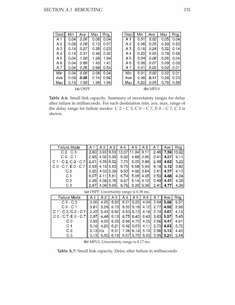
SECTION A.1 REROUTING 131
(a) OSPF (b) MPLS
Table A.6: Small link capacity. Summary of uncertainty ranges for delayafter failure in milliseconds. For each destination min, ave, max, range ofthe delay range for failure modes: C 2 – C 3, C 0 – C 7, E 0 – C 7, C 2 isshown.
(a) OSPF. Uncertainty range is 0.38 ms.
(b) MPLS. Uncertainty range is 0.17 ms.
Table A.7: Small link capacity. Delay after failure in milliseconds

132 CHAPTER A MISCELLANEOUS CORE NETWORK RESULTS
A.1.1.2 Large Link Capacity
(a) OSPF
(b) MPLS
Table A.8: Large link capacity. Uncertainty range for delay before failurein milliseconds
(a) OSPF (b) MPLS
Table A.9: Large link capacity. Uncertainty range for delay after failure inmilliseconds. For each destination min, ave, max, range of the delay rangefor failure modes: C 2 – C 3, C 0 – C 7, E 0 – C 7, C 2 is shown.

SECTION A.1 REROUTING 133
(a) OSPF. Uncertainty range is 0.77 ms.
(b) MPLS. Uncertainty range is 0.83 ms.
Table A.10: Large link capacity. Delay after failure in milliseconds. Uncer-tainty range is 0.77 ms.

134 CHAPTER A MISCELLANEOUS CORE NETWORK RESULTS
A.1.2 Jitter
A.1.2.1 Small Link Capacity
(a) OSPF (b) MPLS
Table A.11: Small link capacity. Uncertainty range for jitter before failurein milliseconds
(a) OSPF (b) MPLS
Table A.12: Small link capacity. Uncertainty range for jitter after failure inmilliseconds. For each destination min, ave, max, range of the delay rangefor failure modes: C 2 – C 3, C 0 – C 7, E 0 – C 7, C 2 is shown.

SECTION A.1 REROUTING 135
(a) OSPF. Uncertainty range is 0.09 ms.
(b) MPLS. Uncertainty range is 0.06 ms.
Table A.13: Small link capacity. Jitter after failure in milliseconds.

136 CHAPTER A MISCELLANEOUS CORE NETWORK RESULTS
A.1.2.2 Large Link Capacity
(a) OSPF
(b) MPLS
Table A.14: Large link capacity. Uncertainty range for jitter before failurein milliseconds
(a) OSPF (b) MPLS
Table A.15: Large link capacity. Uncertainty range for jitter after failure inmilliseconds. For each destination min, ave, max, range of the delay rangefor failure modes: C 2 – C 3, C 0 – C 7, E 0 – C 7, C 2 is shown.

SECTION A.1 REROUTING 137
(a) OSPF. Uncertainty range is 0.002 ms.
(b) MPLS. Uncertainty range is 0.001 ms.
Table A.16: Large link capacity. Jitter after failure in milliseconds.


Appendix B
Miscellaneous Access Network
Results
B.1 Rerouting
(a) Link failures
(b) Node failures
Table B.1: Uncertainty range for RSTP rerouting times in milliseconds
139

140 CHAPTER B MISCELLANEOUS ACCESS NETWORK RESULTS
(a) Link failures
(b) Node failures
Table B.2: Uncertainty range for MPLS effective rerouting in milliseconds,which is a sum of LSP rerouting and LSP setup
(a) Setup
(b) Rerouting
Table B.3: MPLS average setup and rerouting times

SECTION B.2 DELAY 141
B.2 Delay
(a) RSTP. Uncertainty range is 0.38 ms.
(b) MPLS. Uncertainty range is 0.13 ms.
Table B.4: Delay after failure in milliseconds
(a) RSTP (b) MPLS
Table B.5: Summary of uncertainty ranges for delay after failure in mil-liseconds

142 CHAPTER B MISCELLANEOUS ACCESS NETWORK RESULTS
B.3 Jitter
(a) RSTP (b) MPLS
Table B.6: Summary of uncertainty ranges for jitter after failure in mil-liseconds
(a) RSTP. Uncertainty range is 0.38 ms.
(b) MPLS. Uncertainty range is 0.13 ms.
Table B.7: Jitter after failure in milliseconds

Appendix C
Reliability Concepts
Much of the information presented in this chapter comes from Shooman [74],
supported by other references [11, 46, 82, 83].
C.1 Fundamental Concepts
Availability function A(t) is the probability that the system is operational
at time t. With A(250) = 0.95, if 100 units operated for 250 hours, on
average 95 will be operating at the end of that time and 5 units will be
undergoing repair.
Reliability function R(t) is the probability that the system has oper-
ated without failure over the interval [0, t]. With R(250) = 0.95, if 100
units operated during [0, 250] hours time period 95 units will have no
failure and 5 units will have failed at some time.
From the two definitions R(t) ≤ A(t), as reliability is not concerned
with when a unit fails whereas for availability the unit may be fixed be-
fore the time t. Essentially R(t) does not allow for repair and A(t) does.
The special case R(t) = A(t) is when a single unit is irreparable. Re-
143

144 CHAPTER C RELIABILITY CONCEPTS
pairable systems with redundant components do improve R(t). For ex-
ample, a simple two unit parallel system will benefit from repairs as if
unit one fails and gets repaired before the second unit fails the system
will not fail in that time interval.
For networks concepts of availability and reliability are often consid-
ered the same. Steady state availability
Ass = limt→∞
A(t)
is one common measure. A(t) is typically a decreasing function, with
the highest availability of 1 at the start with all units operational. A(t)
decreases with time to some steady value (very close to one in a good
system) called a steady state availability Ass. The reason Ass is used so
frequently is because it gives a lower bound on availability and it is sim-
pler to calculate.
Ass =µ
λ + µis a steady state availability of single component, where
λ is the failure or hazard rate and µ is the repair rate. Ass is often written
as
Availability =Uptime
Downtime + Uptime
Markov modeling is needed in more complicated systems to determine
Ass correctly.
More mathematically,
R(t) = eR
t
0z(ξ)dξ ,where z(t) is the hazard function
In most cases the hazard function is assumed to be constant z(t) = λ.
This makes calculations less complicated and it fits most circumstances

SECTION C.1 FUNDAMENTAL CONCEPTS 145
extremely well. Generally, z(t) follows a bathtub shape. In the early
stages of deployment of an element more failures occur due to new parts
defects, incompatibility, and so on. As time progresses those early fail-
ures disappear and we enter the main lifespan of the element. In this
middle stage relatively few random failures occur at approximately the
same level throughout the time period. In the last stage of the element’s
lifespan wearout failures start to happen and increase at some variable
rate. Thus, if we assume an element always operates in its middle stage,
the constant failure rate assumption should hold.
There are more complex models, such as linear and logarithmic mod-
els, but those are not necessary for the analysis in here. Using a constant
failure rate in the definition of reliability we get R(t) = e−λt.
Hazard rate λ is usually measured in failures in time (FITs) in telecom-
munication industry. One FIT is one failure per a billion hours of opera-
tion. For the earlier example λ = 0.05/250 = 2 × 10−4 = 200, 000 × 10−9
failures per billion hours. Now R(250) = e−2×10−4
× 250 = 0.95, which
agrees with the reliability figure.
Besides reliability Mean Time To Failure (MTTF) is another measure
which can be compared when deciding between different systems. MTTF
can be easier to compute by using Laplace theory. MTTF is defined as
MTTF =
∫ ∞
0
R(t)dt
The MTTF for a single element with reliability expression R(t) = e−λt is
MTTF =
∫ ∞
0
e−λtdt =1
λ

146 CHAPTER C RELIABILITY CONCEPTS
xnx1 x2
Figure C.1: Series configuration
For comparison purposes MTTF of a two element parallel system with
repair is
MTTF =3λ + µ
2λ2
C.2 Basic Network Configurations
C.2.1 Series
A series configuration is one in which its elements are distributed in a
chain, one after another as in Figure C.1. Failure of any one of the ele-
ments will cause system failure. Thus reliability of a series system is R =
P (x1, x2, ...xn) and provided all units are identical R = P (x1)P (x2)...P (xn).
It follows that a series configuration is worse than a single element.
Series configuration is useful when analysing or designing a large sys-
tem. Such system is usually decomposed into a number of subsystems
linked by couplers. In effect the subsystem form a series configuration.
C.2.2 Parallel
A parallel configuration is one in which elements are distributed such
that the only one of the elements is needed to be operational for the sys-
tem to function correctly. Figure C.2 shows a parallel configuration. Re-
liability of a parallel system is the probability of the sum of probabili-
ties must be expanded using Inclusion-Exclusion Principle. Inclusion-

SECTION C.2 BASIC NETWORK CONFIGURATIONS 147
Exclusion Principle is very well known from set theory, it is as follows:
R = P (x1 + x2 + . . . + xj) =∑
1≤i≤j
xi
−∑
1≤l<m≤j
(xl · xm)
+∑
1≤n<o<p≤j
(xn · xo · xp)
...
− (−1)j−1(x1 · x2 · . . . · xj)
For example:
P (x1 + x2 + x3) = x1 + x2 + x3 − x1x2 − x1x3 − x2x3 + x1x2x3
The indecies for each term are given by the number of combinations pos-
sible(
n
k
)
. For example, the second term in the general expression contains(
j
2
)
expressions.
There are two categories of parallel systems. A parallel (or online
or hot standby) system has each of the redundant units operating at all
times. A (cold) standby system is superior since the redundant units are
not powered and so cannot fail. A standby system is superior as time to
system failure of a parallel system is the longest time to failure of one of
n components. In a standby configuration the system failure occurs after
the sum of time to failure of each redundant component.
Both parallel and standby systems have disadvantages. It is rare that
a big system can be constructed using a parallel configuration. Usually it
is several redundant systems joint together by couplers. Even if all those
subsystems employ parallel redundancy, the reliability of the system is

148 CHAPTER C RELIABILITY CONCEPTS
xn
x1
x2
Figure C.2: Parallel configuration
limited to the reliability of the couplers. Calculations show that coupler
reliability must be greater than the reliability of individual components.
Standby systems must switch to use the redundant component in the
presence of failure. Such a switch is never perfect and must detect the fail-
ure of the active element, switch power and I/O to the standby element
efficiently. The effect of the switch is to multiply the existing reliability
by its own.
C.2.3 r-out-of-n
A configuration of units is called r-out-of-n when r units of the total n
units must be functional for the system to continue its operation. When-
ever there are less than r operational units left the system fails. This setup
is a version of parallel redundancy which is more restricted. This type of
redundancy is often employed as it provides big cost savings when com-
pared to a fully redundant parallel setup. Examples of use of the r-out-of-
n system can be found in optical networks with the (N:M) fault-tolerance
scheme, network cabling, and many others.
The reliability expression is governed by the binomial coefficient as
any combination of r out of n units may be operational. Therefore R =
Ps =∑k=r
n
(
n
k
)
pk(1−p)n−k as B(r; n, p) =(
n
k
)
pk(1−p)n−k is the probability
that r units succeed with probability p.

SECTION C.3 RELIABILITY IN GRAPHS 149
C.3 Reliability in Graphs
Reliability of a large network is not easy to assess due to the multiple
number of paths between any two endpoints. A brute force method is
to enumerate each path and do the reliability calculations using all pos-
sible combinations of these paths. For very small network this may be
possible, but for larger structures a method from graph theory is used.
The method uses the notion of tie and cut sets. A tie-set is a set of
branches in the a graph or network connecting two nodes. A cut-set is a
set of branches, which when removed interrupts all connections between
two nodes. Depending on the network topology it may be easier to find
its tie-sets or its cut-sets. Reliability is calculated as follows
R = 1 − Pf = 1 − P (C1 + C2 + . . . + Ci) = P (T1 + T2 + . . . + Tj),
where Ck is the probability of a cut-set and Tl is the probability of a tie-
set. Both probabilities are computed based on the probability of failure
of each network branch and node that is part of the cut-set or tie-set.
It is difficult enough to calculate the reliability between only two nodes.
But in general k-node reliability is required for full assessment of reliabil-
ity. Approximation techniques based on heuristics and graph transfor-
mations exist. The problem is still too extensive to do by hand and a
reliability computer package is likely to be used.
C.3.1 N-modular Redundancy
Practical parallel systems present the difficulties of either couplers in hot
standby system or switches in cold standby system. N-modular redun-

150 CHAPTER C RELIABILITY CONCEPTS
VoterB
A
C
Figure C.3: Triple modular redundancy configuration with a non-redundant voter
1 − (λ + µ)∆t
s0 s1 s2
1
λ∆t λ∆t
µ∆t
1 − λ∆t
Figure C.4: Markov reliability model for two identical parallel elements
dancy is a simpler and more reliable mechanism to deploy a parallel con-
figuration by taking advantage of digital nature of system inputs. The
basic idea is that the same input is used for at least N units, each one
produces and output which is put into a voter. The voter uses majority
voting of its inputs to produce a correct output. Figure C.3 gives the most
common N-modular redundancy scheme, Triple Modular Redundancy
(TMR).
Redundant voters may also be used to improve reliability. Redundant
voters are easier to implement than redundant couplers.
C.4 Markov Modeling
Markov modeling for reliability and availability is described in Chapter
3 and Appendix B of Shooman [74].
The essence of Markov modeling for reliability and availability is to
build a model of states the system can enter and specify transitional prob-
abilities of entering each state.

SECTION C.4 MARKOV MODELING 151
Figure C.4 illustrates the Markov model for a simple two element par-
allel system consists of four states: state s0 with no elements failed; state
s1 with either one elements failed (counts as two); and state s2 with both
elements failed. Transitions from each state are specified by failure rates
λ and repair rates µ. The sum of transitional probabilities at each state
must equal to 1. Once all states and transitions are specified, a system of
first order differential equations with respect to time are written down.
The rules for formulating the differential equations are on pages 113 and
450 of Shooman [74]. The rule can be summarised as equating the deriva-
tive of the probability at any node to the sum of the transmissions coming
into the node (or equivalently, transmissions coming out, with an oppo-
site sign in front). The initial conditions for the model is that we start
with a good system so probability of the first state is 1. The probability of
all other states is set to 0. Solution to such a system of first order differen-
tial equations can be arrived at using a technique of Laplace transforms,
which convert the differential system (in time domain) into algebraic set
of equations (referred to as frequency domain). The new set of equations
is solved and then transferred back to time domain. Mathematics com-
puter packages such as Maple, Matlab, or Mathematica are likely to be
used for systems with more than four states.
A slightly different Markov model is needed to calculate availability.
The difference is that a repair transition from the system down state is
allowed. The change to Figure C.4 is the addition of s2 → s1 transition
with a new repair rate. The rest of the procedure remains the same as for
reliability calculation, with the outcome being an availability function.
To calculate Ass several methods exist. One of the simpler methods
is setting each time derivative to 0 in the system of differential equations

152 CHAPTER C RELIABILITY CONCEPTS
formed from the Markov graph.
Markov models can deal with different failures such as coverage (de-
tection) failures and recovery failures. This is done by adding more states
representing different failures and adding appropriate transitions. Chap-
ters 3 and 4 of Ali [11] give examples of such models in the context of
switching systems.
C.5 Fault-Tree Analysis
To analyse a system it needs to be decomposed into either a reliability
block diagram or a fault tree [74].
Reliability block diagram diagrams represent elements and their con-
nections. Configurations such as series or parallel can be recognised from
such a diagram and appropriate calculations can be made.
Fault tree diagrams represent different failure modes of the system
and its parts. Failure modes that lead to specific effects are organised in
a hierarchical tree diagram. A failure at one level of the tree may trigger
another failure one level above it. In such manner chains of events may be
carefully traced with probabilities assigned to effects from failure modes
and hazards. fault trees provide a view of how the system may fail from
the failure modes point of view, rather than physical layout of elements
shown by a reliability block diagram.
C.6 Failure Mode and Effect Analysis
Failure mode and effect analysis is a tabular procedure that identifies
single-event chains that trigger distinct failures. Such analysis is done

SECTION C.7 RELIABILITY OPTIMISATION 153
early in the design process and serves as an input for many further pro-
cedures such as constructing fault trees, reliability block diagrams, and
testing.
C.7 Reliability Optimisation
In this context optimisation means to design the system with the best
possible reliability or availability given some constraints. Often only the
financial cost constraint is used, but there are other often implicit con-
straints including network topology, time, and complexity.
To optimise reliability or availability in a complex system the system
must be decomposed or apportioned into subsystem, which can in turn
be optimised. Chapter 7 of Shooman [74] discusses reliability optimisa-
tion and states five main approaches to apportionment.
Equal weighting apportionment states that each subsystem must have
the same reliability. This is an easy first attempt to apportionment.
Relative difficulty method improves on equal weighting by factoring
in relative cost and difficulty of each subsystem. Usually rough heuristics
are used to estimate costs and difficulty.
Relative failure rates apportionment requires knowledge of failure
rates of each subsystem. The method is easier than relative difficulty and
is likely to be more accurate.
Albert’s method is an algorithm for apportionment. First an estimate
of each subsystem reliability is needed, with the system reliability lower
than the target. The subsystems that need to have a higher reliability
than estimated to meet the target have their reliability increased so that
they are equal. The algorithm is a good way to calculate the minimum

154 CHAPTER C RELIABILITY CONCEPTS
reliability of the subsystems required to meet the target system reliability
(rather than trial and error).
Finally apportionment can be multi-layered in large systems. In such
cases stratified optimisation is used, which reiterates optimisation in re-
quired subsystems. Engineering process of building a system is usually
a trial-and-error process. This is due to many parameter being unknown
prior to the design, difficult constraints, estimation of maintenance costs
and knock-on effects, and so on. Thus often upper and lower bounds on
the design are calculated using the techniques for apportionment. Sev-
eral designs can then be modeled to give reliability within the bounds.
The best design in terms of reliability and all the constraints is selected.
C.8 Network Reliability Implementation
This section shows how the theoretical network reliability computation
was implemented in this thesis.
According to Section C.2.2, the general method for working out reli-
ability between two points in a network is to compute the probability of
the sum of all paths probabilities. All paths between source and destina-
tion must be found, where a path is a sequence of links and nodes from
source to destination without visiting the same node more than once.
Practically this posed two problems. First, all the correct paths must
be found. Second, the probability of the sum of the path individual re-
liabilities must be calculated. The first problem was solved recursively
as most standard graph algorithms, with graph construction such that
no loops were allowed in a path. The second problem is more difficult

SECTION C.8 NETWORK RELIABILITY IMPLEMENTATION 155
than appears, because the probability of the sum of probabilities must be
expanded using Inclusion-Exclusion Principle, stated in Section C.2.2.
To implement the Inclusion-Exclusion expansion an algorithm from
Rosen [67] was used to systematically generate all combinations of n ele-
ments, taken k at a time, that is(
n
k
)
. This way each term in the expression
can be generated. The pseudocode is shown below:
1: list of individual probabilities2: for all i such that 1 ≤ i ≤ listSize do3: Compute all combinations of size i out of listSize,
(
ilistSize
)
{Using implementation of Rosen [67] algorithm}4: for all combinations of size i do5: for all indecies in one combination do6: Multiply appropriate values in list
7: end for8: Add the combination to the totalProb with appropriate sign9: end for
10: end for11: return totalProb
Figure C.5: Inclusion-Exclusion Principle implementation
Figure C.5 is exact, but it is solving an NP-hard problem, for which
any exact solution is exponential in the number of input elements. This
means that for a medium to large network the method takes too long
to compute the answer. In complex networks, such as electricity grids
and PSTN, complicated (unpublished) heuristic algorithms are used. The
execution time of such heuristics depends on the required precision of the
answer. Investigation of such heuristics and their efficiencies is not part
of my thesis.
Top Related