


Languages
Pages
Legal


Joao Alberto Vieira de Campos Pereira Claro
Multiobjective Metaheuristic Approaches
for Mean-Risk Combinatorial Optimisation
with Applications to Capacity Expansion
Dissertacao apresentada a Faculdade de Engenharia da Universidade do Porto
para obtencao do grau de Doutor em Engenharia Electrotecnica e de Computadores
e realizada sob a orientacao cientıfica do Professor Doutor Jorge Manuel Pinho de Sousa,
Professor Associado da Faculdade de Engenharia da Universidade do Porto
Departamento de Engenharia Electrotecnica e de Computadores
Faculdade de Engenharia da Universidade do Porto
2007

O trabalho de investigacao apresentado nesta dissertacao foi parcialmente enquadrado
no projecto FCT POCI/EGE/61362/2004.
ii

a Teresa
ao Daniel
ao Pedro
a Ana
a Maria
iii

iv

Resumo
Muitas decisoes em Gestao de Operacoes, em particular a um nıvel estrategico, sao
tomadas na presenca de incerteza. Tendo em conta o impacto destas decisoes, a
questao do risco esta surpreendentemente ausente da maioria da investigacao e do
trabalho aplicado nesta area. Tal podera ser parcialmente explicado pela complexi-
dade dos modelos de optimizacao para estes problemas, uma vez que necessitam de
incluir parametros incertos, variaveis de decisao logicas ou outras de natureza discreta,
e mais do que um objectivo.
Uma das areas de decisao crıticas no ambito da Estrategia de Operacoes e a area
da Expansao de Capacidade, que se ocupa das decisoes quanto ao tipo, dimensao,
calendarizacao e localizacao dos investimentos em capacidade. Os modelos de ca-
pacidade tem de tratar diversas questoes relacionadas com a complexidade acima
referida, questoes estas que conduzem a nao-linearidades, nao-convexidades, integra-
lidade e objectivos multiplos.
Por outro lado, as meta-heurısticas multiobjectivo sao algoritmos de optimizacao
com caracterısticas que favorecem uma aplicacao extremamente eficiente em proble-
mas com estas dificuldades, tendo, por este motivo, o potencial de vir a assumir um
papel importante como abordagens genericas para problemas de optimizacao combi-
natoria simultaneamente envolvendo a optimizacao do valor medio dos resultados e a
minimizacao do risco. O principal objectivo deste trabalho foi realizar uma avaliacao
preliminar deste potencial.
v

Na primeira parte desta dissertacao, apresenta-se uma abordagem de meta-heurısticas
multiobjectivo baseadas em pesquisa local para uma formulacao media-risco de um
problema da mochila estocastico estatico, considerando uma versao exacta e uma
versao com aproximacao amostral do problema, e a variancia e o valor em risco
condicional como medidas de risco.
A segunda parte deste trabalho debruca-se sobre uma formulacao media-risco para
um problema de investimento em capacidade multi-perıodo, com irreversibilidade, in-
divisibilidade e economias de escala nos custos de capacidade. E, para este problema,
proposta uma abordagem de meta-heurısticas multiobjectivo baseadas em pesquisa
local, considerando o valor em risco condicional como medida de risco.
Na terceira parte da dissertacao, introduz-se flexibilidade de processo no problema
tratado na segunda parte, o que conduz, em cada perıodo, a decisoes de natureza
discreta relativas ao investimento em expansao de capacidade, e decisoes de natureza
contınua relativas a utilizacao da capacidade disponıvel para satisfazer a procura. Os
problemas de utilizacao de capacidade sao resolvidos com programacao linear, com
o objectivo de determinar a capacidade mınima exigida para cada recurso, quando
os restantes permanecem inalterados, disponibilizando, assim, informacao sobre a
admissibilidade das decisoes de investimento. A este problema sao aplicadas meta-
heurısticas multiobjectivo baseadas em pesquisa local (em que novamente se considera
o valor em risco condicional como medida de risco).
Os estudos computacionais realizados indicam claramente que as abordagens de-
senvolvidas sao capazes de produzir aproximacoes aos conjuntos eficientes media-risco
de elevada qualidade, com um esforco computacional modesto. Fica, assim, validada
a hipotese de que as meta-heurısticas multiobjectivo constituem uma classe de algo-
ritmos apropriados para lidar com as dificuldades apresentadas pelos problemas de
optimizacao combinatoria media-risco.
vi

Abstract
Many decisions in Operations Management, in particular at a strategic level, are
made in the presence of uncertainty. Considering the impact of these decisions, risk
concerns are surprisingly absent in the majority of research and applied work in this
area. This may be partially explained by the complexity of optimisation models for
these problems, as they must include uncertain parameters, logical or other discrete
decision variables, and more than one objective.
One of the critical decision areas within Operations Strategy is Capacity Expan-
sion, which is concerned with deciding the type, magnitude, timing, and location of
capacity acquisition. Capacity models are required to address a variety of problem
features related to the previously mentioned complexity, these features leading to
nonlinearities, nonconvexities, integrality and multiple objectives.
On the other hand, multiobjective metaheuristics are optimisation algorithms ex-
tremely well suited to efficiently tackle problems that present these difficulties. They
have therefore the potential to play an important role as general approaches for combi-
natorial optimisation problems simultaneously dealing with the optimisation of mean
results and the minimisation of risk. The primary objective of our work was to per-
form a preliminary assessment of this potential.
In the first part of this dissertation, we present a multiobjective local search
metaheuristic approach for both exact and sample approximation versions of a mean-
risk static stochastic knapsack problem, considering both variance and conditional
vii

value-at-risk as risk measures.
The second part of this work is concerned with a mean-risk multistage capacity
investment problem with irreversibility, lumpiness and economies of scale in capac-
ity costs. We propose a multiobjective local search metaheuristic approach for this
problem, considering conditional value-at-risk as a risk measure.
In the third part of the dissertation, we introduce process flexibility in the problem
addressed in the second part, leading to the consideration, in each period, of discrete
decisions concerning the investment in capacity expansion, and continuous decisions
concerning the utilization of the available capacity to satisfy demand. We solve the
capacity utilization problems with linear programming, in order to find the minimum
capacity for each resource with the other resources remaining unchanged. In this way,
information is provided on the feasibility of the discrete investment decisions. We
apply a multiobjective local search metaheuristic to this problem, again considering
conditional value-at-risk as a risk measure.
Results of computational studies are presented, that clearly indicate the designed
approaches are capable of producing high-quality approximations to the mean-risk
efficient sets, with a modest computational effort, thus validating the hypothesis that
multiobjective metaheuristics are a class of algorithms well suited to deal with the
difficulties presented by mean-risk combinatorial optimisation problems.
viii

Resume
Beaucoup de decisions en Gestion des Operations, en particulier au niveau strategique,
sont prises en presence d’incertitude. En considerant l’impact de ces decisions, c’est
surprenant que la question du risque soit absente de la majorite de la recherche et
du travail applique dans ce domaine. Ceci peut etre partiellement explique par la
complexite des modeles d’optimisation pour ces problemes, qui demandent l’inclusion
de parametres incertains, variables de decision logiques ou autres de nature discrete,
et plusieurs objectifs.
Un des principaux secteurs de decision en Strategie des Operations, c’est celui
de l’Expansion de Capacite, qui s’occupe des decisions sur le type, la dimension, le
calendrier et la localisation des investissements en capacite. Les modeles de capacite
doivent considerer plusieurs aspects lies a la complexite mentionnee, aspects qui con-
duisent a l’existence de non-linearites et de non-convexites, a l’integralite des variables
et a des objectifs multiples.
D’autre part, les metaheuristiques multiobjectif sont des algorithmes d’optimisation
tres bien adaptes a la resolution efficace des problemes avec ces difficultes, et elles
ont, pour cette raison, le potentiel de jouer un role important comme approches
generiques pour des problemes d’optimisation combinatoire traitant simultanement
l’optimisation de la moyenne des resultats et la minimisation du risque. Le principal
objectif de notre travail a ete de realiser une evaluation preliminaire de ce potentiel.
Dans la premiere partie de ce travail, nous presentons une approche de meta-
ix

heuristiques multiobjectif basees sur recherche locale pour une formulation moyenne-
risque d’un probleme de sac a dos stochastique statique, en considerant une version
exacte et une version avec approximation par echantillonnage, et la variance et la
valeur a risque conditionnelle comme mesures de risque.
La deuxieme partie de ce travail aborde une formulation moyenne-risque pour un
probleme d’investissement en capacite multiperiode, avec irreversibilite, indivisibilite
et economies d’echelle dans les couts de capacite. Pour ce probleme, nous proposons
une approche de metaheuristiques multiobjectif basees sur recherche locale, en con-
siderant la valeur a risque conditionnelle comme mesure de risque.
Dans la troisieme partie de ce travail, nous ajoutons flexibilite de processus au
probleme aborde dans la deuxieme partie, ce qui nos mene a considerer, dans chaque
periode, des decisions de nature discrete associees a l’investissement en expansion de
capacite, et des decisions de nature continue associees a l’utilisation de la capacite
disponible pour satisfaire la demande. Nous resolvons les problemes d’utilisation de
capacite par programmation lineaire, pour trouver le minimum de capacite requis pour
chaque ressource, tandis que les autres ressources sont fixees. Cette procedure fournit
de l’information sur l’admissibilite des decisions d’investissement. Nous appliquons a
ce probleme des metaheuristiques multiobjectif basees sur recherche locale, en con-
siderant encore la valeur a risque conditionnelle comme mesure de risque.
Les etudes computationnelles realisees indiquent clairement que les approches
developpees sont capables de produire des approximations aux ensembles efficaces
moyenne-risque de qualite, avec un petit effort computationnel, en validant l’hypothese
de que les metaheuristiques multiobjectif sont des algorithmes d’optimisation tres
bien adaptes pour traiter les difficultes presentees par les problemes d’optimisation
combinatoire moyenne-risque.
x

Agradecimentos
Ao Prof. Jorge Pinho de Sousa, por me ter acolhido no seu grupo de investigacao, por
me ter colocado em contacto com as areas de aplicacao e as ferramentas abordadas
neste trabalho, pelo incentivo a explorar a ideia de aplicar meta-heurısticas multi-
objectivo a problemas de optimizacao combinatoria media-risco, e pela orientacao
paciente de um aluno de doutoramento frequentemente em orbita.
Ao Prof. Rui Guimaraes e ao Prof. Jose Fernando Oliveira, pelas oportunidades
de ensino que evoluıram para uma posicao a tempo inteiro na Universidade.
Ao Jose Fernando, ao Miguel e ao Ricardo, pelas muitas proveitosas discussoes e
sugestoes.
Ao Jorge, por ser mais do que um orientador, por ser um amigo.
Aos meus pais e as minhas irmas, pelas minhas raızes.
A Teresa, ao Daniel, ao Pedro, a Ana e a Maria, por um amor alem do amor.
A um Amor Supremo.
xi

xii

Acknowledgements
To Prof. Jorge Pinho de Sousa, for receiving me in his research group, for introducing
me to the application areas and the tools considered in this work, for the incentive to
explore the idea of applying multiobjective metaheuristics to mean-risk combinatorial
optimisation problems, and for the patient guidance of a PhD student frequently in
orbit.
To Prof. Rui Guimaraes and Prof. Jose Fernando Oliveira, for the teaching
opportunities that evolved into a full-time position in the University.
To Jose Fernando, Miguel and Ricardo, for the many helpful discussions and
suggestions.
To Jorge, for being more than an advisor, for being a friend.
To my parents and my sisters, for my roots.
To Teresa, Daniel, Pedro, Ana and Maria, for a love beyond love.
To a Love Supreme.
xiii

xiv

Contents
1 Introduction 1
1.1 Research Opportunity . . . . . . . . . . . . . . . . . . . . . . . . . . 1
1.2 Research Strategy . . . . . . . . . . . . . . . . . . . . . . . . . . . . . 2
1.3 Structure of the Dissertation . . . . . . . . . . . . . . . . . . . . . . . 4
2 Some Fundamental Concepts, Tools and References 5
2.1 Multiobjective Combinatorial Optimisation . . . . . . . . . . . . . . . 6
2.2 Multiobjective Metaheuristics . . . . . . . . . . . . . . . . . . . . . . 9
2.3 MetHOOD - a Metaheuristic Framework . . . . . . . . . . . . . . . . 14
2.3.1 Object-Oriented Software . . . . . . . . . . . . . . . . . . . . 14
2.3.2 Object-Oriented Approaches for Metaheuristics . . . . . . . . 15
2.3.3 MetHOOD . . . . . . . . . . . . . . . . . . . . . . . . . . . . . 15
2.3.4 MOLS Template . . . . . . . . . . . . . . . . . . . . . . . . . 16
2.3.5 Implementation of PSA and TAMOCO . . . . . . . . . . . . . 17
2.3.6 Neighbourhood Variation . . . . . . . . . . . . . . . . . . . . . 18
2.4 Risk Measures . . . . . . . . . . . . . . . . . . . . . . . . . . . . . . . 19
2.4.1 Definitions of Risk Measures . . . . . . . . . . . . . . . . . . . 19
2.4.2 Stochastic Dominance . . . . . . . . . . . . . . . . . . . . . . 21
2.4.3 Coherence . . . . . . . . . . . . . . . . . . . . . . . . . . . . . 22
2.4.4 Computing CVaRα via Linear Programming . . . . . . . . . . 23
xv

2.5 Capacity Expansion . . . . . . . . . . . . . . . . . . . . . . . . . . . . 24
2.5.1 Background . . . . . . . . . . . . . . . . . . . . . . . . . . . . 24
2.5.2 Relevant Literature . . . . . . . . . . . . . . . . . . . . . . . . 25
2.5.3 A Multistage Stochastic Integer Programming Model . . . . . 26
2.5.4 Challenges in Capacity Expansion . . . . . . . . . . . . . . . . 29
3 A Multiobjective Metaheuristic for a Mean-Risk Static Stochastic
Knapsack Problem 31
3.1 Introduction . . . . . . . . . . . . . . . . . . . . . . . . . . . . . . . . 32
3.2 The Static Stochastic Knapsack Problem with Random Weights . . . 33
3.2.1 Problem Description . . . . . . . . . . . . . . . . . . . . . . . 33
3.2.2 Mean-Risk Models . . . . . . . . . . . . . . . . . . . . . . . . 34
3.2.3 Sample Approximation . . . . . . . . . . . . . . . . . . . . . . 37
3.2.4 Exact Objective Functions with Independent Normal Weights 39
3.3 Related Work . . . . . . . . . . . . . . . . . . . . . . . . . . . . . . . 40
3.3.1 Static Stochastic Knapsack Problem . . . . . . . . . . . . . . 40
3.3.2 Optimisation with Risk Measures . . . . . . . . . . . . . . . . 41
3.3.3 Applications of Metaheuristics . . . . . . . . . . . . . . . . . . 42
3.4 A Multiobjective Metaheuristic Approach . . . . . . . . . . . . . . . 46
3.5 Computational Study . . . . . . . . . . . . . . . . . . . . . . . . . . . 49
3.5.1 Instances . . . . . . . . . . . . . . . . . . . . . . . . . . . . . 49
3.5.2 Performance Evaluation . . . . . . . . . . . . . . . . . . . . . 50
3.5.3 Study of Sample Approximation . . . . . . . . . . . . . . . . . 51
3.5.4 Algorithm Configuration . . . . . . . . . . . . . . . . . . . . . 53
3.5.5 Experimental Results . . . . . . . . . . . . . . . . . . . . . . . 54
3.6 Conclusions . . . . . . . . . . . . . . . . . . . . . . . . . . . . . . . . 57
xvi

4 A Multiobjective Metaheuristic for a Mean-Risk Multistage Capac-
ity Investment Problem 59
4.1 Introduction . . . . . . . . . . . . . . . . . . . . . . . . . . . . . . . . 59
4.2 Related Work . . . . . . . . . . . . . . . . . . . . . . . . . . . . . . . 61
4.3 A Mean-Risk Model . . . . . . . . . . . . . . . . . . . . . . . . . . . 63
4.4 A Multiobjective Metaheuristic Approach . . . . . . . . . . . . . . . 66
4.4.1 Solution . . . . . . . . . . . . . . . . . . . . . . . . . . . . . . 69
4.4.2 Capacity Variation (CV) Neighbourhood . . . . . . . . . . . . 69
4.4.3 Expansion Shift (ES) Neighbourhood . . . . . . . . . . . . . . 74
4.4.4 Initial Solutions . . . . . . . . . . . . . . . . . . . . . . . . . . 74
4.4.5 Objective Functions . . . . . . . . . . . . . . . . . . . . . . . 75
4.5 Computational Study . . . . . . . . . . . . . . . . . . . . . . . . . . . 75
4.5.1 Test Instances . . . . . . . . . . . . . . . . . . . . . . . . . . . 75
4.5.2 Algorithm Configuration . . . . . . . . . . . . . . . . . . . . . 77
4.5.3 Experimental Results . . . . . . . . . . . . . . . . . . . . . . . 77
4.6 Conclusions . . . . . . . . . . . . . . . . . . . . . . . . . . . . . . . . 78
5 A Multiobjective Metaheuristic for a Mean-Risk Multistage Capac-
ity Investment Problem with Process Flexibility 81
5.1 Introduction . . . . . . . . . . . . . . . . . . . . . . . . . . . . . . . . 82
5.2 Related Work . . . . . . . . . . . . . . . . . . . . . . . . . . . . . . . 83
5.3 Mathematical Programming Models . . . . . . . . . . . . . . . . . . . 85
5.4 A Multiobjective Metaheuristic Approach . . . . . . . . . . . . . . . 90
5.4.1 Basic Concepts . . . . . . . . . . . . . . . . . . . . . . . . . . 92
5.4.2 Solution . . . . . . . . . . . . . . . . . . . . . . . . . . . . . . 94
5.4.3 Capacity Variation (CV) Neighbourhood . . . . . . . . . . . . 95
5.4.4 Expansion Shift (ES) Neighbourhood . . . . . . . . . . . . . . 99
xvii

5.4.5 Initial Solutions . . . . . . . . . . . . . . . . . . . . . . . . . . 100
5.4.6 Objective Functions . . . . . . . . . . . . . . . . . . . . . . . 101
5.5 Computational Study . . . . . . . . . . . . . . . . . . . . . . . . . . . 101
5.5.1 Instances . . . . . . . . . . . . . . . . . . . . . . . . . . . . . 101
5.5.2 Algorithm Configuration . . . . . . . . . . . . . . . . . . . . . 103
5.5.3 Experimental Results . . . . . . . . . . . . . . . . . . . . . . . 104
5.6 Conclusions . . . . . . . . . . . . . . . . . . . . . . . . . . . . . . . . 106
6 Conclusion 109
6.1 Background . . . . . . . . . . . . . . . . . . . . . . . . . . . . . . . . 109
6.2 Main Contributions . . . . . . . . . . . . . . . . . . . . . . . . . . . . 110
6.3 Future Developments . . . . . . . . . . . . . . . . . . . . . . . . . . . 111
xviii

List of Tables
2.1 Definitions of risk measures . . . . . . . . . . . . . . . . . . . . . . . 20
3.1 Instance parameters . . . . . . . . . . . . . . . . . . . . . . . . . . . 49
3.2 Average approximation quality gap (%) as function of number of sce-
narios . . . . . . . . . . . . . . . . . . . . . . . . . . . . . . . . . . . 52
3.3 Standard deviation of approximation quality gap (%) as function of
number of scenarios . . . . . . . . . . . . . . . . . . . . . . . . . . . . 52
3.4 Algorithm configurations for instances with 25 items . . . . . . . . . 53
3.5 Algorithm configurations for instances with 250 items . . . . . . . . . 53
3.6 Results of computational study for exact instances with 25 items . . . 54
3.7 Results of computational study for approximate instances with 25 items 55
3.8 Results of computational study for approximate instances with 250 items 56
4.1 Instance parameters . . . . . . . . . . . . . . . . . . . . . . . . . . . 75
4.2 Algorithm configurations . . . . . . . . . . . . . . . . . . . . . . . . . 78
4.3 Computational study . . . . . . . . . . . . . . . . . . . . . . . . . . . 79
5.1 Instance parameters . . . . . . . . . . . . . . . . . . . . . . . . . . . 102
5.2 Algorithm configurations . . . . . . . . . . . . . . . . . . . . . . . . . 104
5.3 Computational study for instances with 4 periods and time limit 300 s 105
xix

5.4 Computational study for instances with 4 periods and neighbourhood
CV(15)→ES(15) . . . . . . . . . . . . . . . . . . . . . . . . . . . . . 105
5.5 Computational study for instances with 5 periods and time limit 3600 s 106
5.6 Computational study for instances with 5 periods and neighbourhood
CV(15)→ES(15) . . . . . . . . . . . . . . . . . . . . . . . . . . . . . 106
xx

List of Figures
2.1 The MetHOOD framework . . . . . . . . . . . . . . . . . . . . . . . . 16
2.2 MOLS class diagram . . . . . . . . . . . . . . . . . . . . . . . . . . . 17
2.3 PSA and TAMOCO derived from the MOLS template . . . . . . . . 18
2.4 Class diagram for neighbourhood variation . . . . . . . . . . . . . . . 19
2.5 Scenario tree for expansion costs . . . . . . . . . . . . . . . . . . . . . 28
3.1 The MetHOOD framework . . . . . . . . . . . . . . . . . . . . . . . . 48
3.2 Hypervolume indicator . . . . . . . . . . . . . . . . . . . . . . . . . . 50
3.3 Average approximation quality gap as function of the number of scenarios 52
3.4 Nondominated sets and approximation sets of different quality gap levels 57
4.1 Solution and demand constraints . . . . . . . . . . . . . . . . . . . . 64
4.2 Solution and cost structure . . . . . . . . . . . . . . . . . . . . . . . . 65
4.3 The MetHOOD framework . . . . . . . . . . . . . . . . . . . . . . . . 68
4.4 Solution before positive capacity variation . . . . . . . . . . . . . . . 70
4.5 Solution after positive capacity variation . . . . . . . . . . . . . . . . 71
4.6 Solution before negative capacity variation . . . . . . . . . . . . . . . 72
4.7 Solution after negative capacity variation . . . . . . . . . . . . . . . . 73
4.8 Hypervolume indicator . . . . . . . . . . . . . . . . . . . . . . . . . . 76
5.1 Solution and capacity constraints . . . . . . . . . . . . . . . . . . . . 86
xxi

5.2 Capacity expansions and cost structure . . . . . . . . . . . . . . . . . 87
5.3 Capacity utilization and demand constraints . . . . . . . . . . . . . . 88
5.4 The MetHOOD framework . . . . . . . . . . . . . . . . . . . . . . . . 92
5.5 Capacity, K∗i,n, excess of capacity over K∗
i,n, backward and forward
capacity surplus . . . . . . . . . . . . . . . . . . . . . . . . . . . . . . 94
5.6 Solution after positive capacity variation . . . . . . . . . . . . . . . . 96
5.7 Solution after negative capacity variation . . . . . . . . . . . . . . . . 98
5.8 Hypervolume indicator . . . . . . . . . . . . . . . . . . . . . . . . . . 103
xxii

List of Algorithms
1 ε-constraint method . . . . . . . . . . . . . . . . . . . . . . . . . . . . 8
2 Pareto Simulated Annealing . . . . . . . . . . . . . . . . . . . . . . . . 11
3 Tabu Search for Multiobjective Combinatorial Optimisation . . . . . . 12
4 Multiobjective Local Search Template . . . . . . . . . . . . . . . . . . 13
5 Multiobjective Local Search Template . . . . . . . . . . . . . . . . . . 47
6 Multiobjective Local Search Template . . . . . . . . . . . . . . . . . . 67
7 Multiobjective Local Search Template . . . . . . . . . . . . . . . . . . 91
xxiii

xxiv

Quisiera a veces borrar todos mis versos
para escribir por primera vez un poema.
Todo lo escrito no me alcanza
para sentir que he escrito uno.
Tampoco es suficiente haber vivido:
vivir comienza siempre ahora.
Roberto Juarroz
Decimotercera Poesıa Vertical
xxv

xxvi

Chapter 1
Introduction
1.1 Research Opportunity
A large number of decisions in Operations Management are made in the presence
of uncertainty. In fact, key factors, such as prices, resource availability or product
demand, are regularly characterised by uncertainty. Considering the importance of
many of these decisions, in particular at a strategic level, the amount of attention
given to incorporating risk in the decision processes is surprisingly small. This may
be partially explained by the complexity of optimisation models for these problems,
as they include uncertain parameters, logical or other discrete decision variables, and
more than one objective. Analytical tractability is hindered by this complexity, and
even if mixed integer stochastic programming models can be developed, no efficient
generic algorithms exist to solve them.
An important area where these issues are critical is the area of Capacity Expan-
sion, in Operations Strategy. Capacity models are required to address a variety of
problem features directly related to the abovementioned complexity. Partial or com-
plete irreversibility of the investments, uncertainty in future rewards, some latitude
on the timing or dynamics of the investments, multidimensionality of the invest-
1

2 Introduction
ments, indivisibility of capacity expansions, fixed costs, economies of scale, the need
to explicitly consider risk - the presence of these characteristics results, among other
difficulties, in the presence of nonlinearities, nonconvexities, integrality and multiple
objectives.
Metaheuristics are optimisation algorithms extremely well suited to efficiently
tackle problems that present these features. In particular, multiobjective metaheuris-
tics can be quite effective in simultaneously handling objectives reflecting both risk
and, as traditionally, expected results. The application of multiobjective metaheuris-
tics to mean-risk combinatorial optimisation problems is an unexplored research area,
whose potential can thus be significant.
1.2 Research Strategy
Given the embryonic state of the research in this area, the primary objective of our
work was to perform a preliminary assessment of multiobjective metaheuristics in
solving mean-risk combinatorial optimisation problems.
This assessment was performed over a set of problems selected to represent the
characteristics of the problems in the field:
• static single period structure, with all decisions made upfront, and dynamic
multiperiod structure, with future opportunities for decisions that may use new
information available up to the moment;
• binary, integer and mixed integer decision variables;
• linear, quadratic, closed-form and numerical objectives;
• expectation and classic (variance) and more recent (conditional value-at-risk)
risk measures as objectives.

1.2 Research Strategy 3
We have also tried to select problems exclusively related to Capacity Expansion,
but were unsuccessful in finding a binary problem in this area. The three selected
problems are the following:
• The Static Stochastic Knapsack Problem, a static binary problem, that we con-
sider in an exact formulation, with numerical objectives, and in a sample approx-
imation formulation, with closed-form linear and quadratic objectives. Both
variance and conditional value-at-risk are considered as risk measures in both
formulations.
• The Multistage Capacity Investment Problem, a dynamic integer problem, with
uncertainty incorporated in the model by a scenario tree, and discrete capacity
investment decision variables. Conditional value-at-risk is considered as a risk
measure.
• The Multistage Capacity Investment Problem with Process Flexibility, a dynamic
mixed integer problem, where uncertainty again is modelled by a scenario tree.
Capacity investment decision variables are discrete, whereas capacity allocation
decision variables are continuous. Conditional value-at-risk is again considered
as a risk measure.
An object-oriented framework with multiobjective metaheuristics, that we have
developed in previous work, was used in designing and implementing approaches for
these problems. The ILOG CPLEX Mixed Integer Programming solver was used
to obtain the mean-risk reference solution sets for randomly generated instances of
all problems, except for the exact and variance formulations of the Static Stochastic
Knapsack Problem, that required the use of a solution enumeration procedure. The
performance of the developed metaheuristic approaches, in terms of solution qual-
ity and computational time, was then evaluated through a series of computational
experiments.

4 Introduction
1.3 Structure of the Dissertation
Chapter 2 is an introduction to some fundamental topics, aiming at providing the
background for the research presented in this dissertation.
Chapters 3, 4 and 5 are related but self-contained essays that have been individ-
ually submitted for publication in international journals, currently being object of
reviewing procedures. They have been slightly rearranged for inclusion in this dis-
sertation, but the content has suffered no modifications. Chapter 3 is devoted to the
Static Stochastic Knapsack Problem, chapter 4 to the Multistage Capacity Invest-
ment Problem, and chapter 5 to the Multistage Capacity Investment Problem with
Process Flexibility.
Chapter 6 concludes the dissertation, presenting the key contributions of this
research and suggesting future developments.
The option to provide self-contained essays in chapters 3, 4 and 5 entails some
content repetition, namely of the following topics: description of the multiobjective
local search template and overview of the object-oriented framework; description
of performance measures; review of related work regarding optimisation with risk
measures and metaheuristics for stochastic optimisation and portfolio selection; and
definition of risk measures. This option, however, hopefully makes each of these
chapters more accessible and readable.

Chapter 2
Some Fundamental Concepts,
Tools and References
To help make this dissertation as self-contained as possible, we present in this chapter
an introduction to some basic topics, and provide interested readers with a compre-
hensive set of relevant literature references. These topics are: fundamental concepts
in multiobjective combinatorial optimisation; multiobjective metaheuristics, with an
emphasis on multiobjective local search based approaches; the overall architecture
of the MetHOOD object-oriented framework, highlighting the multiobjective local
search template and the support for neighbourhood variation; an overview of the risk
measures that are more commonly discussed in the literature and the prevailing con-
cepts of adequacy of risk measures; a short review of results on capacity expansion,
with some basic literature references, and additional references that suggest and vali-
date the pertinence of the developments that we have proposed. A section is included
for each of these topics.
5

6 Some Fundamental Concepts, Tools and References
2.1 Multiobjective Combinatorial Optimisation
A Combinatorial Optimisation (CO) problem is a mathematical optimisation problem
with a discrete set of feasible solutions. It can be defined generically in the following
way: given a discrete set S and a function f : S → R, find x∗ ∈ S such that
f (x∗) = min {f (x) | x ∈ S} . (2.1)
x is a feasible solution, S is the solution space or decision space and f is the
objective function. It is common and, in a certain way, natural to formulate a CO
problem as an Integer Programming (IP) problem, in which the solutions are described
by vectors of integer variables and the solution space is described by a set of equality
and inequality constraints.
In terms of computational complexity, many CO problems are NP-hard, which
reflects their intrinsic difficulty and justifies the adoption in practice of heuristic,
non-optimising approaches.
Many practical problems, usefully modelled as CO problems, often require an
evaluation of solutions according to a number of different perspectives. Multiobjective
Combinatorial Optimisation (MOCO) problems can be represented by the following
generic model:
min f1 (x) = z1
...
min fk (x) = zk
s.t. x ∈ S,
(2.2)
where x is a feasible solution, S is the discrete solution space, and f1, ..., fk are the ob-
jective functions. z = (z1, . . . , zk) is called a criterion vector. The feasible region in the
objective space is Z ={z ∈ Rk : zi = fi (x) ,x ∈ S
}or Z =
{z ∈ Rk : z = f (x) ,x ∈ S
},
considering a vector function f (x) = (f1 (x) , . . . , fk (x)). z ∈ Z is nondominated if

2.1 Multiobjective Combinatorial Optimisation 7
and only if there is no other z′ ∈ Z such that z′i ≤ zi, ∀i, and z′i < zi, for some i. The
nondominated set consists of all nondominated criterion vectors. x ∈ S is efficient
if and only if its image in the objective space is nondominated. The efficient set
consists of all efficient solutions.
It is often useful to work with similar ranges of values in all objectives. Such
rescaling may be achieved by applying range equalisation factors. Accordingly, each
objective zi is multiplied by its corresponding range equalisation factor
πi =1
Ri
[k∑
j=1
1
Rj
]−1
, (2.3)
where Ri is the range width of the ith criterion value over the efficient set.
As an important part of several methods for MOCO, scalarising functions can
be used for mapping criterion vectors to values in an ordinal scale of quality. The
weighted sum scalarising function sws (z, z0, λ) =∑k
i=1 λi (zi − z0i ), considers a ref-
erence criterion vector z0 and strictly positive scalar weights λi. The weighted sum
problem can be defined as
min sws (z, z0, λ)
s.t. z ∈ Z.(2.4)
The optimal criterion vectors in this problem are designated as supported non-
dominated. Other nondominated criterion vectors are referred to as nonsupported
nondominated. In linear multiobjective optimisation problems there are no nonsup-
ported nondominated criterion vectors. However, in integer or nonlinear multiob-
jective problems, the existence of nonsupported nondominated criterion vectors is
common.
For MOCO problems, the ε-constraint method considers single-objective problems
constructed from the original multiobjective problem, where only one of the objective
functions is kept as an objective, while the others are transformed into constraints

8 Some Fundamental Concepts, Tools and References
(that implicitly define their levels of achievement). By performing a systematic vari-
ation of the bounds of these constraints, this method is able to find both supported
and nonsupported efficient solutions. For a bi-objective problem
min f1 (x) = z1
min f2 (x) = z2
s.t. x ∈ S,
(2.5)
we use the implementation of this method outlined in Algorithm 1, where δ is a
positive constant small enough to avoid missing any efficient solutions.
Algorithm 1: ε-constraint method
Initialise the efficient set E = {};x1 = min f1 (x) , s.t. x ∈ S;while x1 6= {} do
x2 = min f2 (x) , s.t. f1 (x) = f1 (x1) ,x ∈ S;Insert x2 in E;x1 = min f1 (x) , s.t. f2 (x) ≤ f2 (x2)− δ,x ∈ S;
end
The use of metrics, for measuring distances between criterion vectors plays a
fundamental role in several MOCO methods. The Manhattan metric defines the
distance between two criterion vectors, z1 and z2, by
‖z1 − z2‖π1 =
k∑i=1
πi|z1i − z2
i |, (2.6)
considering range equalisation factors πi.

2.2 Multiobjective Metaheuristics 9
2.2 Multiobjective Metaheuristics
The difficulty in solving many practical CO problems has led to important research
efforts in the development of more efficient approaches, reflected in significant reduc-
tions in computational requirements. Among these are heuristics - simple algorithms,
frequently based in common sense, that are able to find a good (not necessarily op-
timal) solution for difficult problems, in a fast and easy way - and metaheuristics -
master strategies that guide and modify other heuristics to produce solutions beyond
those that can be produced by a search for local optima (Glover, 1986).
To a large extent, the success in applying metaheuristics to single-objective CO
problems is due to features such as their general applicability, the flexibility to han-
dle specific constraints in real world problems, and the interesting trade-off between
solution quality and computation, development and implementation effort (Pirlot,
1996). Many of these methods also present a high robustness concerning the features
of problem instances or parameter tuning. Tabu Search (TS), Simulated Annealing
(SA) and Genetic Algorithms (GA) are metaheuristics that are currently broadly
used, and described in mainstream Operations Research textbooks.
These same features have been fostering their application in MOCO, enabling the
handling of variations in problem formulation or in the objectives. Surveys on mul-
tiobjective metaheuristics (MOMH) are available in Ehrgott and Gandibleux (2000),
Jones et al. (2002) and Ehrgott and Gandibleux (2004). GA have led the way in
this area, the pioneer work of Schaffer with the Vector Evaluated Genetic Algorithm
(Schaffer, 1985) dating back to 1985. The early survey on multiobjective GA in
Fonseca and Fleming (1995) points out that GA seem specially fit for use in multiob-
jective contexts for two main reasons: working with a population of solutions, they
can search for the multiple solutions of the efficient set in parallel, eventually exploring
similarities among them; also, they are less sensitive than traditional mathematical

10 Some Fundamental Concepts, Tools and References
programming techniques to the issues of shape and continuity of the nondominated
set.
This second feature is shared with SA and TS based approaches. One group of
these approaches (Serafini, 1992; Ulungu et al., 1998; Gandibleux et al., 1997) is based
on repeated executions of the single-objective metaheuristic, with a combination of
the objectives in an aggregating function, usually a weighted sum scalarising function.
A search direction is established by the weights in this function, whose variation in
each execution aims at enabling a complete approximation of the nondominated set.
In another group, that includes Pareto Simulated Annealing (PSA) (Czyzak and
Jaszkiewicz, 1998) and Tabu Search for Multiobjective Combinatorial Optimisation
(TAMOCO) (Hansen, 2000), the first mentioned feature is introduced in SA and TS
based approaches, through the consideration of a population of solutions, each one
holding its own set of weights. These weights are dynamically computed so that each
solution moves towards the nondominated frontier and away from other solutions in
the population, that are nondominated with respect to it.
In PSA (Algorithm 2) the weights for each solution are updated according to
the relation between the components of the corresponding criterion vector and the
nearest nondominated criterion vector. The distance between criterion vectors may
be measured with a Manhattan metric. A constant multiplying factor α, or its inverse
1/α, are used to update the weights, with α higher than, but close to, 1 (e.g., 1.05).
The weights are incorporated in the acceptance probability, that can be defined as
the minimum of the weighted acceptance probabilities for each objective
minj=1,...,k
{min {1, exp (∆zi,j/T )}λi,j
}. (2.7)
Increasing the weight associated to an objective reduces the probability of accepting
movements that do not improve that objective and increases the probability of im-

2.2 Multiobjective Metaheuristics 11
Algorithm 2: Pareto Simulated Annealing
Generate a set of initial feasible solutions G ⊂ S;Initialise the approximation to the efficient set E = {};foreach xi ∈ G do
Update E with xi;endInitialise temperature T ;while a stopping criterion is not met do
foreach xi ∈ G doSelect solution xw ∈ G, such that f (xw) is nearest to and nondominated by f (xi);if xw does not exist or first iteration with xi then
Generate random weights λi,j for the weight vector λi associated with xi, suchthat λi,j ≥ 0 and
∑kj=1 λi,j = 1;
endelse
foreach objective function fj doif fj (xi) ≤ fj (xw) then λi,j = αλi,j ;else λi,j = λi,j/α;
endNormalise weights λi,j so that
∑kj=1 λi,j = 1;
endRandomly select xs ∈ Neighbourhood (xi);if f (xs) is nondominated by f (xi) then update E with xs;Randomly select a value p ∈ [0; 1];if p ≤ P (f (xi) , f (xs) , T, λi) then xi = xs;
endUpdate temperature T ;
end
proving that objective. The temperature starts at an initial value T0 and, at every L
iterations, is multiplied by a constant positive value lower than 1.
In TAMOCO (Algorithm 3) the vector of weights is used to define a direction of
optimisation for each solution, towards the nondominated set and away from other
nondominated solutions, in proportion to their proximity. Proximity can be defined
as the inverse of distance, which in turn can be measured with a Manhattan metric,
considering range equalisation factors. In the absence of better knowledge, range
equalisation factors can be computed from the objective ranges in the approximation
set.

12 Some Fundamental Concepts, Tools and References
Algorithm 3: Tabu Search for Multiobjective Combinatorial Optimisation
Generate a set of initial feasible solutions G ⊂ S;Initialise the vector of range equalisation factors π with πj = 1/k;Initialise the approximation to the efficient set E = {};foreach xi ∈ G do
Initialise the corresponding tabu list TLi = {};Update E with xi;
endwhile a stopping criterion is not met do
foreach xi ∈ G doInitialise the corresponding weight vector λi = 0;foreach xl ∈ G such that f (xl) is nondominated by and different from f (xi) do
Compute proximity w = g (d (f (xi) , f (xl) , π));foreach objective function fj such that fj (xi) < fj (xl) do
λi,j = λi,j + πjw;endNormalise weights λi,j so that
∑kj=1 λi,j = 1;
endif λi = 0 then
Generate random weights λi,j for the weight vector λi associated with xi, suchthat λi,j ≥ 0 and
∑kj=1 λi,j = 1;
endSelect xs ∈ Neighbourhood (xi) , such thatλi · f (xs) ≤ λi · f (xt) , ∀xt ∈ Neighbourhood (xi) , and(TLi does not make (xi,xs) tabu or xs satisfies the aspiration criterion );Insert attributes of (xi,xs) at the end of TLi, removing the first element if TLi isfull;xi = xs;Update E with xs;Update π;
endif a drift criterion is met then
Replace a randomly selected solution with another randomly selected solution in G;end
end
To avoid the concentration of solutions in certain areas, a drift mechanism is used,
whereby a randomly selected solution is replaced with a copy of another randomly
selected solution. The aspiration criterion consists of accepting any efficient solution.
PSA and TAMOCO can be viewed as Multiobjective Local Search (MOLS) pro-
cedures. Both aim at producing a good approximation of the efficient set, working
with a population of solutions, each solution holding a weight vector for the definition

2.2 Multiobjective Metaheuristics 13
Algorithm 4: Multiobjective Local Search Template
Generate a set of initial feasible solutions G ⊂ S;Initialise the approximation to the efficient set E = {};foreach xi ∈ G do
Initialise the corresponding context;Update E with xi;
endwhile a stopping criterion is not met do
foreach xi ∈ G doUpdate the corresponding weight vector λi;Initialise the selected solution xs = 0;foreach x′ ∈ Neighbourhood(xi) do
Update E with x′;if x′ is selectable and x′ is preferable to xs then xs = x′;
endif xs 6= 0 and xs is acceptable then xi = xs;
endend
of a search direction. Each approach proposes a different strategy for the definition
of the weights, but share identical purposes for that definition: orientation of the
search towards the nondominated frontier and spreading of solutions over that fron-
tier (the former is achieved by the use of positive weights, while the latter is based
on a comparison with other solutions of the population). Although in different ways,
both methods operate on each single solution, searching and selecting a solution in
its neighbourhood that will eventually replace it. Each procedure involves traditional
metaheuristic components such as neighbourhoods, in general, or tabu lists, in the
specific case of TAMOCO. The identification of these common aspects has suggested
the definition of a MOLS template (Algorithm 4), as a way to provide a generic basis
for designing different specific algorithms.

14 Some Fundamental Concepts, Tools and References
2.3 MetHOOD - a Metaheuristic Framework
2.3.1 Object-Oriented Software
Four essential principles of the object-oriented paradigm are data encapsulation, data
abstraction, inheritance and polymorphism. The object is the unit of data encapsula-
tion, consisting of a set of variables and a set of methods used to alter and access those
variables. An object accepts messages that invoke methods. An object’s signature
is the set of messages it accepts. A class is a data abstraction, expressing aspects
that are common to identical objects, and taking the form of a template to create
a particular kind of object. Class inheritance allows a set of classes to share parts
of a common signature or implementation (variables and methods). Polymorphism
is essential to code reuse, by enabling methods to take objects of different types as
arguments.
Reusable object-oriented software has been made available mainly through class
libraries and frameworks. A class library packages together a set of classes, eventually
structured using inheritance, from which an application can be built. A framework
can be defined as a set of classes that embodies an abstract design for solutions to a
family of related problems (Johnson and Foote, 1988). One main difference between
these two concepts is that frameworks provide default behaviour, while with class
libraries, all the collaboration between components usually has to be defined. Frame-
works provide design reuse, an area where another domain has also gained particular
significance - Design Patterns, which are descriptions of communicating objects and
classes that are customised to solve a general design problem in a particular context
(Gamma et al., 1994).

2.3 MetHOOD - a Metaheuristic Framework 15
2.3.2 Object-Oriented Approaches for Metaheuristics
The two main incentives for developing object-oriented approaches for metaheuristics
have been bringing theory and applications closer, by developing simply structured,
open-ended systems, that incorporate theoretical results (Nievergelt, 1994), and facili-
tating the implementation and comparison of methods, through increased modularity,
rational order and reusability of software structures (Ferland et al., 1996). Several
object-oriented approaches for metaheuristics have been presented in the literature.
Descriptions of some of some of the most prominent can be found, in detail, in Voss
and Woodruff (2002) or, in a brief introduction, in Fink et al. (2002).
2.3.3 MetHOOD
MetHOOD (MetaHeuristics Object-Oriented Development) is a framework for MOMH
that extensively incorporates design patterns in its design (Claro and Sousa, 2001).
At the time the MetHOOD framework was proposed, no other object-oriented ap-
proaches for MOMH had been reported in the literature. Still in 2001, a C++ class
library for MOMH, developed by Andrzej Jaszkiewicz, was made publicly available
at http://www-idss.cs.put.poznan.pl/∼jaszkiewicz/MOMHLib/. In a 2004 re-
view of heuristics and metaheuristics designed for the solution of MOCO problems
(Ehrgott and Gandibleux, 2004) MetHOOD was still the only work cited in the area
of reusable MOMH software.
MetHOOD has been used to support the applications described in the following
chapters and in its present state of development, provides (Figure 2.1): support for
the definition of the variable parts of the problem domain, related to solutions, move-
ments, increments and evaluating functions; support for problem data; a template
and a concrete implementation of a constructive algorithm; a MOLS template and
the derivations of PSA and TAMOCO from this template; extensions for a candidate

16 Some Fundamental Concepts, Tools and References
Problem data support
Basic structures and relations
Basic algorithms SolversConstructivealgorithms
Provided by the client
Extensions for basic and constructive algorithms, and solvers
IncrementsSolutionsEvaluationsMovementsData
Figure 2.1: The MetHOOD framework
list strategy and a neighbourhood variation strategy; a solver level for the articula-
tion of constructive and MOLS algorithms, and the implementation of a high-level,
parallel, hybridisation strategy.
2.3.4 MOLS Template
Figure 2.2 presents the class diagram for the MOLS template part of the framework.
A MOLS algorithm (MOLocalSearch) iterates over a population (PopulationInitial)
of solutions (Solution), building an approximation to the efficient set (EfficienSet)
of the considered problem. A neighbourhood (Neighbourhood) is created for each
solution, with the services of a neighbourhood prototype (NeighbourhoodPrototype).
For each solution, the algorithm obtains all the movements (MovementCurrent) in the
neighbourhood and selects one (MovementSelected). The neighbourhood is traversed
with a movement iterator (MoveIterator), that sees the neighbourhood as a move-
ment container (MoveContainer). The efficient set is updated with all generated
movements. Movement selection always involves the solution’s weights, which are
defined by a weight definition strategy (WeightDefinition), taking into consideration
the solutions from a larger population (PopulationLarger). This larger population

2.3 MetHOOD - a Metaheuristic Framework 17
methood::EfficientSet
methood::Population
methood::Solution
1 *
methood::Movement
methood::MOLocalSearch
methood::MoveGeneratormethood::Neighbourhood
methood::SolutionContext
methood::MOLSSolContext
1
1* 1
1
1
*
1
*
1
1
1
1
1methood::WeightDefinition
1
1
methood::RangeEqFactors
1
1
methood::MovementFilter
*1
methood::MoveContainer
1 1
1
1CurrentSelected Prototype
*
1Base
1Base
*
Initial1
1
Larger1
*
*
1
*
1
Prototype
methood::Ranges
1
1
* 1
methood::MoveIterator
* 1
*
1
1 1
*
1
Figure 2.2: MOLS class diagram
contains the population of the algorithm, and may also contain other solutions, such
as reference solutions, or solutions being worked on by other algorithms.
2.3.5 Implementation of PSA and TAMOCO
Figure 2.3 illustrates the differences in the way that PSA (MOSimAnneal) and
TAMOCO (MOTabuSearch) implement the definition of several of the template’s
primitive operations: weight vectors are distinctly initialised and updated (for PSA
PSAWeightDef , and for TAMOCO MOTSWeightDef); the neighbourhood in PSA
is a random subneighbourhood with just one movement; the selection of a gener-
ated movement (+IsMovementV alid()) in TAMOCO considers tabu status, aspira-
tion criteria, and a comparison of evaluations based on a weighted sum scalarising

18 Some Fundamental Concepts, Tools and References
#candidate_list#candidateList#curPopulation#current+found_list#largerPopulation#neighbourhood#obtained#pSol#ranges#REF#REqWeights#selected+ulMaxIter
methood::MOLocalSearch
#Nbh#obtained#selected...
+Initialize ()+Iterate()+isEnd()+Search()+isMovementValid()+UpdateREQWeights()+Selectable()+Select()+Acceptable()
+IterativeProcess()+Finalize()+GetIter()+Go()-IncIter()+Initialize ()+isEnd()+Iterate()+Update()
-ulIter
methood::IterativeProcess
+isMovementValid ()
methood::MovementFilter
Initialize();while(!isEnd()){ Iterate(); Update(); IncIter();}Finalize();
pSol=curPopulation->begin();while(pSol!=curPopulation->end()){current=*pSol; DefineWeights(current,largerPopulation,REF); MoveIterator->First(); while(!MoveIterator->IsDone()) { obtained = MoveIterator->Current(); efficientSet->Update(current,obtained); if(!Selectable(obtained)) delete obtained; MoveIterator->Next(); } selected = Select(); if(selected!=0 && Acceptable(selected)) selected->ExecuteOn(current); delete selected; pSol++;}return Nbh->Selectable(Move);
return Nbh->Select();
methood::MOTabuSearchmethood::MOSimAnneal
+Initialize ()+Update()+Acceptable()+isMovementValid()
+Initialize ()+Update()+Acceptable()+isMovementValid()
methood::AspirationCriteria
methood::CoolingSchedule
methood::TabuMemory
methood::SolutionContextmethood::Solution
1 1
methood::MOLSSolContext
methood::TabuSolContext
Criar contextoCriar lista tabuChamar inicialização deMOLocalSearch
if(isNotTabu(move) || AspirationCriteriaHolds(move) ) return true;else return false;
InsertInTabuMemory(move);return true;
Drift
111
1
11
Pesos aleatórios para todas as soluçõesArrancar esquema dearrefecimentoChamar inicializaçãode MOLocalSearch
Incrementar esquemade arrefecimentoChamar update deMOLocalSearch
Aceitar movimento deacordo com cálculo daprobabilidade de aceitação
return true;
* 1
methood::WeightDefinition
1
1
methood::PSAWeightDef methood::MOTSWeightDef
Create contextCreate tabu listCall initialization of MOLocalSearch
Random weights for all solutionsStart cooling scheduleCall intialization of MOLocalSearch
Increment cooling scheduleCall update of MOLocalSearch
Accept movement according to acceptance probability\
Figure 2.3: PSA and TAMOCO derived from the MOLS template
function, while in PSA a generated movement is always selected; the acceptance
(+Acceptable()) of a selected movement in PSA is a function of an acceptance prob-
ability, while in TAMOCO a selected movement is always accepted.
2.3.6 Neighbourhood Variation
The framework also provides support for neighbourhood variation (Figure 2.4), by
considering a sequence of neighbourhood structures (vector < MoveGenerator >)
and using them dinamically according to the evolution of the search process: if a new

2.4 Risk Measures 19
methood::Neighbourhood
methood::VariableNeighbourhood
methood::MoveGenerator
*
1
vector<MoveGenerator>
1 1..*
1
1
aMoveGenerator1 aMoveGenerator2 aMoveGenerator3
vector<MoveGenerator>::iterator
1 1*
1
*
1
methood::Evaluation
1
-Previous1
Figure 2.4: Class diagram for neighbourhood variation
accepted solution is preferable to the current one, or if the current neighbourhood is
the last in the sequence, the first neighbourhood in the sequence will be used next;
otherwise the following neighbourhood in the sequence will be used next.
2.4 Risk Measures
2.4.1 Definitions of Risk Measures
The identification of adequate risk measures is currently a field of very active research,
that we will not review in detail in this work. This section is a very short introduction
to the basic concepts of risk measurement, aiming at providing an adequate context
for the work that is presented ahead.
Measuring risk requires that a correspondence ρ is established between a space
X of random variables and a nonnegative real number, i.e., ρ : X → R+0 . Scalar
measures of risk allow ordering and comparison according to risk values. Most of the
basic ideas for risk measures arise from the consideration of dispersion parameters,
excess probabilities, quantiles or conditional expectations.

20 Some Fundamental Concepts, Tools and References
For a presentation of some of the fundamental concepts in risk measures, we
consider a continuous loss random variable X with distribution function FX and
density function fX . The expected value of X can be defined in the following way
E [X] =
∫xfX (x) dx. (2.8)
Table 2.1 presents some of the risk measures that are more commonly discussed
in the literature((·)+ = max {·, 0}).
Table 2.1: Definitions of risk measures
Risk measure Definition
Variance E[(X − E [X])2]
Mean absolute deviation E [|X − E [X]|]p-th semideviation from target t
(E
[(X − t)p
+
])1/p
p-th central semideviation(E
[(X − E [X])p
+
])1/p
Gini mean difference∫
E[(ξ −X)+
]dFX (ξ)
α-value-at-risk (VaRα) inf {x|FX (x) > α}α-conditional value-at-risk (CVaRα) E [X|X ≥ VaRα [X]]
To be able to handle possible discontinuities, the definition of CVaRα must replace
the original conditional expectation by the following α-tail expectation
CVaRα [X] =∫
xdFαX (x) ,
where F αX (x) =
0 if FX (x) < α
FX(x)−α1−α
if FX (x) ≥ α
.(2.9)
The prevailing concepts of adequacy of risk measures are consistency with sto-
chastic dominance (Ogryczak and Ruszczynski, 1999) and coherence (Artzner et al.,
1999).

2.4 Risk Measures 21
2.4.2 Stochastic Dominance
The stochastic dominance (Ogryczak and Ruszczynski, 1999) relations between two
random variables are defined by pointwise comparison of performance functions based
on their distribution functions. The first function F(1)X is just the distribution function
F(1)X (x) = FX (x), and the weak (º) and strict (Â) relations of the first degree
stochastic dominance (FSD) are defined as follows:
X ºFSD Y ⇔ FX (z) ≥ FY (z) ,∀z ∈ R.
X ÂFSD Y ⇔ X ºFSD Y and Y �FSD X.(2.10)
FX (x) expresses the probability of having losses below a given target value x. If
X ÂFSD Y , then X is preferred to Y within all models preferring smaller losses,
regardless of risk-aversion.
The second function F(2)X is given by the area below the distribution function
FX (x):
F(2)X (x) =
∫ x
−∞FX (z) dz, x ∈ R. (2.11)
The weak and strict relations of the second degree stochastic dominance (SSD)
are defined as follows:
X ºSSD Y ⇔ F(2)X (z) ≥ F
(2)Y (z) ,∀z ∈ R.
X ÂSSD Y ⇔ X ºSSD Y and Y �SSD X.(2.12)
If X ÂSSD Y , then X is preferred to Y within all risk-averse preference models
that prefer smaller losses. Consistency with SSD is therefore a fundamental aspect
in risk comparison.
Consistency with stochastic dominance has been studied in the literature mainly
considering the following definition: a risk measure ρ is α-consistent with stochastic

22 Some Fundamental Concepts, Tools and References
dominance of order p iff
X ºp Y ⇒ E (X) + αρ (X) ≤ E (Y ) + αρ (Y ) . (2.13)
The α-consistency with stochastic dominance of order p implies α′-consistency
with stochastic dominance of order p, for all α′ such that 0 < α′ ≤ α (Ogryczak
and Ruszczynski, 1999). A risk measure ρ is consistent with stochastic dominance of
order p iff it is α-consistent with stochastic dominance of order p for all α ∈ R+.
In general, variance and mean absolute deviation are not consistent with FSD
or SSD (see, e.g., Markert (2004)). p-th central semideviation is 1-consistent with
stochastic dominance of order 1, ..., p + 1 (Ogryczak and Ruszczynski, 1999) and the
same result applies to Gini’s mean difference (Yitzhaki, 1982). p-th semideviation
from target t is consistent with FSD and SSD, for all p ∈ N (Fishburn, 1977). VaR is
consistent with FSD, but not SSD, whereas CVaR is consistent with both (Ogryczak
and Ruszczynski, 2002).
2.4.3 Coherence
A risk measure ρ : X→ R is coherent (Artzner et al., 1999) if it satisfies the following
properties:
• Translation invariance: ρ (X + a) = ρ (X) + a,∀X ∈ X,∀a ∈ R.
• Subadditivity : ρ (X + Y ) ≤ ρ (X) + ρ (Y ) ,∀X,Y ∈ X.
• Monotonicity : if X ≤ Y, then ρ (X) ≥ ρ (Y ) , ∀X, Y ∈ X.
• Positive homogeneity : ρ (λX) = λρ (X) s,∀X ∈ X,∀λ > 0.
In general, variance, mean absolute deviation, p-th central semideviation and
Gini’s mean difference are not coherent, and p-th semideviation from target t requires

2.4 Risk Measures 23
adaptation of the target to the random variable to be coherent (Markert, 2004). VaR
is not coherent (Artzner et al., 1999). CVaR is coherent (Rockafellar and Uryasev,
2002).
2.4.4 Computing CVaRα via Linear Programming
The properties referred above partially justify the increasing attention that CVaRα
has been receiving in the literature. Another important reason for this attention is
the fact that it can be computed via linear programming. The problem of minimising
CVaRα can be formulated as follows (Rockafellar and Uryasev, 2002):
min ξ + 1(1−α)N
∑Nj=1 Zj
s.t. Zj ≥ f (x, ωj)− ξ, j = 1, ..., N
x ∈ S, Zj ≥ 0, ξ ≥ 0,
(2.14)
where x is a solution, S is the solution space, ω is the randomness component
with a certain probability distribution, ωj are scenarios of ω, j = 1, ..., N, and f (x, ω)
is a loss function. If f (x, ω) is linear and S is described with linear constraints, the
problem of minimising CVaRα is a linear programming problem.
CVaRα constraints can also be considered, as in the following formulation for the
minimisation of the mean loss, with a bound of C for the CVaRα:
min 1N
∑Nj=1 f (x, ωj)
s.t. ξ + 1(1−α)N
∑Nj=1 Zj ≤ C
Zj ≥ f (x, ωj)− ξ, j = 1, ..., N
x ∈ S, Zj ≥ 0, ξ ≥ 0.
(2.15)

24 Some Fundamental Concepts, Tools and References
2.5 Capacity Expansion
2.5.1 Background
A recent review of capacity expansion literature (Julka et al., 2007) identifies the
first recognition of the importance of capacity expansion in Operations Strategy in
Wheelwright (1978), where it was regarded as one of the five strategic manufactur-
ing decision areas, and cites Rudberg and Olhager (2003) to report that substantial
subsequent research has provided wide support for this view. This decision area still
remains crucial, particularly for manufacturing corporations with global production
facilities (Julka et al., 2007) and in high-tech industries such as semiconductor, con-
sumer electronics, telecommunications and pharmaceutical (Wu et al., 2005).
In a 2003 landmark review on strategic capacity management under uncertainty
(Van Mieghem, 2003), capacity expansion has been defined as being concerned with
deciding the type, magnitude, timing, and location of capacity acquisition: these deci-
sions about processing resources in a network play a fundamental role in defining the
network’s capabilities, and are associated with decisions on the types and the levels of
investment. Three very important characteristics are present in investment, in vary-
ing degrees (Dixit and Pindyck, 1994): partial or complete irreversibility, uncertainty
over the future rewards and some latitude on the timing or dynamics of the invest-
ment. A fourth characteristic is added in Van Mieghem (2003): multidimensionality,
i.e., the possibility of investing in resources with different financial and operational
properties. This review also points out additional fundamental challenges in capacity
cost modelling - indivisibility of capacity expansions and nonconvexity arising, e.g.,
from fixed costs or economies of scale - and the surprising fact that few papers on
capacity investment tackle issues related to risk, even if we are often facing significant
investments with uncertain future rewards.

2.5 Capacity Expansion 25
2.5.2 Relevant Literature
Recently the research on capacity expansion has been concerned with the development
of models and techniques that are able to deal with this difficult set of characteristics.
We have found in Ahmed et al. (2003) and Ahmed and Sahinidis (2003) fundamental
references for our work, since the authors have put forward capacity expansion models
that incorporate several of the characteristics pointed out above: irreversibility, un-
certainty, latitude on the timing of investments, multidimensionality and nonconvex
cost functions.
Those authors have divided the previous relevant literature in three main groups:
• Early approaches based on stochastic control theory. These approaches use sim-
ple stochastic processes to model demand, for analytical tractability. Manne
(1961) is the first reference on dynamic capacity models with stochastic de-
mand. Other references are Freidenfelds (1980),Davis et al. (1987) and Bean
et al. (1992).
• Two-stage stochastic programming. Eppen et al. (1989) use standard mixed inte-
ger programming to solve a two-stage stochastic programming model with fixed
charge expansion cost functions, incorporating elements of scenario planning,
integer programming and risk analysis, for strategic capacity planning in the
automotive industry. Berman et al. (1994) apply a two stage stochastic model
with linear costs to capacity expansions in services, using Lagrangian relaxation.
Fine and Freund (1990) formulate and study a product-flexible capacity invest-
ment model as a two-stage nonlinear stochastic program, but assuming linearity
in the cost functions. Liu and Sahinidis (1996) propose a two-stage stochastic
programming approach for process planning under uncertainty, extending a de-
terministic mixed-integer linear programming formulation to account for the
presence of discrete random parameters and subsequently devising a decompo-

26 Some Fundamental Concepts, Tools and References
sition algorithm for the solution of the stochastic model. Swaminathan (2000)
provides heuristics for a two-stage model applied to tool capacity planning in
the semiconductor industry, under uncertainty in demand and with capacity
decisions in the first stage.
• Multistage stochastic programming. Rajagopalan et al. (1998) develop a dy-
namic programming algorithm for a multi-stage capacity acquisition and re-
placement problem, where capacity availability is anticipated, but its magnitude
and timing are uncertain. Chen et al. (2002) use Lagrangian decomposition to
solve a problem of multistage stochastic capacity expansion with technology
selection.
2.5.3 A Multistage Stochastic Integer Programming Model
Addressing the limitations identified in this body of research, those authors propose
a multistage stochastic integer programming model, with a scenario tree to model the
stochastic evolution of costs and demand, and fixed-charge cost functions to model
economies of scale. This model is tackled with approximation and reformulation
schemes that lead to significant improvements on the computational times obtained
by a straightforward use of IP solvers.
The more generic model presented in Ahmed and Sahinidis (2003), addresses the
problem of determining the timing and the level of capacity acquisitions for a set
of production facilities I, as well as an allocation of capacity to satisfy the demand
of a set of product families J . The capacity expansion and allocation decisions are
made with the objective of minimising the expected total discounted investment and
allocation cost, for a discretised planning horizon.
The product demands (d), fixed and variable costs of capacity acquisition (α and
β), and the costs of allocating capacity to products (γ) are assumed to be stochastic.

2.5 Capacity Expansion 27
Uncertainty is modelled as a multilayered tree, whose levels correspond to time peri-
ods. The nodes at a certain tree level constitute the states of the world that can be
distinguished by information available up to that period. T (n) denotes the subtree
rooted in node n, with n = 0 being the root node, and P (n) the path from the root
node to node n. The probability associated with the state of the world in node n is
pn
S is the set of leaf nodes, each related to one of the S scenarios. A scenario
corresponds to a path from the root to a leaf, representing a joint realisation of the
uncertain parameters over all time periods, i.e., for the scenario corresponding to a
leaf node m ∈ S, {dj,n, αi,n, βi,n, γi,j,n}n∈P(m), where i ∈ I and j ∈ J .
Figure 2.5 presents an example of a binary scenario tree, displaying the expansion
costs for a problem with 4 facilities and 3 time periods. In each node the left column
shows the fixed costs, and the right column the variable costs. Each row corresponds
to a different facility. To each arc is associated the probability of the node where the
arc is directed to.
In each node n ∈ T (0), each facility i ∈ I is characterised by a discounted fixed
cost αi,n and a discounted variable cost βi,n of expansion. The capacity expansions
are (deterministically) bounded by Mi,n. The initial capacities are zero, but the
adaptations to include initial capacities are straightforward. The demand for product
j ∈ J is given, in each node, by dj,n. Each unit of capacity of facility i can produce
qi,j units of product j, and the discounted cost associated with this allocation in node
n is γi,j,n.
The decision variables are xi,n, the capacity expansion for facility i at node n,
and wi,j,n, the number of units of capacity of facility i allocated to the production
of product j in node n. The binary variables yi,n take the value 1 if the capacity of
facility i is expanded in node n, and the value 0 otherwise.

28 Some Fundamental Concepts, Tools and References
t=0 t=1 t=2
0.5
0.5
0.25
0.25
0.25
0.25
1
1
2
3
4
5
2
1
3
4
3
6
1
1
2
5
4
6
1
2
3
3
5
6
1
1
3
4
4
5
2
1
3
4
3
7
1
1
2
3
5
8
0
1
2
3
5
6
4
26
25
26
37
25
45
36
Figure 2.5: Scenario tree for expansion costs
This problem can be formulated as follows:
min∑m∈S
pm
∑
n∈P(m)
∑i∈I
(αi,nyi,n + βi,nxi,n +
∑j∈J
(γi,j,nwi,j,n)
)
s.t. xi,n ≤ Mi,nyi,n, n ∈ T (0) , i ∈ I∑i∈I
qi,jwi,j,n ≥ dj,n, n ∈ T (0) , j ∈ J∑j∈J
wi,j,n ≤∑
o∈P(n)
xi,o, n ∈ T (0) , i ∈ I
xi,n ≥ 0, n ∈ T (0) , i ∈ Iyi,n ∈ {0, 1} , n ∈ T (0) , i ∈ I
wi,j,n ≥ 0, n ∈ T (0) , i ∈ I, j ∈ J .
(2.16)
The first set of constraints define yi,n in terms of variables xi,n and establish the

2.5 Capacity Expansion 29
bounds for capacity expansions. The second and third sets of constraints are the
demand satisfaction and capacity constraints, respectively.
2.5.4 Challenges in Capacity Expansion
Lumpiness and the explicit consideration of risk are critical practical issues mentioned
in Van Mieghem (2003) that are not properly addressed in the literature, and whose
importance is reinforced by the survey on capacity management in high-tech industries
by Wu et al. (2005), that confirms the relevance of those features for capacity decisions
in such industries.
In the most recent review of capacity expansion literature, Julka et al. (2007)
identify a primary research opportunity in developing models to simultaneously han-
dle the multiple factors that are relevant in the decision making processes involved in
capacity expansion. As Van Mieghem (2003) concludes, ”Fortunately and unfortu-
nately, capacity-portfolio models rapidly become complex. Complexity is unfortunate
because it often makes superior analytical solutions elusive. Thus, simulation-based
optimization becomes the natural second-best option and is expected to increase in
popularity. At the same time, complexity is fortunate as study is worthwhile with a
potential impact on practice. Compared to the impact of financial portfolio analysis,
even a fraction would be substantial.”

30 Some Fundamental Concepts, Tools and References
Chapter 3
A Multiobjective Metaheuristic for
a Mean-Risk Static Stochastic
Knapsack Problem
(Under review at Computational Optimization and Applications)
In this paper we address two major challenges presented by stochastic discrete op-
timisation problems: the multiobjective nature of the problems, once risk aversion
is incorporated, and the frequent difficulties in computing exactly, or even approx-
imately, the objective function. The latter has often been handled with methods
involving sample average approximation, where a random sample is generated so that
population parameters may be estimated from sample statistics - usually the expected
value is estimated from the sample average. We propose the use of multiobjective
metaheuristics to deal with these difficulties, and apply a multiobjective local search
metaheuristic to both exact and sample approximation versions of a mean-risk static
stochastic knapsack problem. Variance and conditional value-at-risk are considered
as risk measures. Results of a computational study are presented, that indicate the
31

32 A MOMH for a Mean-Risk Static Stochastic Knapsack Problem
approach is capable of producing high-quality approximations to the efficient sets,
with a modest computational effort.
3.1 Introduction
A large number of decisions in Operations Management are made in the presence
of uncertainty. In fact, key factors, such as prices, resource availability or product
demand, are regularly characterised by uncertainty. Considering the importance of
many of these decisions, in particular at a strategic level, the amount of attention
given to incorporating risk in the decision processes is surprisingly small. This may
be partially explained by the complexity of optimisation models for these problems,
as they include uncertain parameters, logical or other discrete decision variables, and
more than one objective.
Even if these problems can be formulated as mixed integer stochastic programming
problems, no efficient generic algorithms exist to solve them, in spite of the recent
increase in the attention given to integrality in the stochastic programming literature.
Research on the application of metaheuristics to these problems, on the other hand,
has either focused on single objective problems or had very confined applications,
particularly in the areas of robust optimisation and portfolio selection.
In this paper we perform a preliminary assessment of multiobjective metaheuristics
for tackling stochastic combinatorial optimisation problems, by applying a multiobjec-
tive local search metaheuristic to a problem with the previously mentioned difficulties
- the static stochastic knapsack problem - that we cast in a mean-risk framework. We
use two different risk measures - variance and conditional value-at-risk - and consider
an exact version of the problem, where expectation and risk measures are computed
exactly, and a sample approximation version, where those values are computed from
a random sample of scenarios.

3.2 The Static Stochastic Knapsack Problem with Random Weights 33
Section 3.2 of the paper describes the problem and presents its several formula-
tions in a mean-risk framework. Section 3.3 surveys related work on the problem,
namely optimisation with risk measures and applications of metaheuristics to sto-
chastic optimisation, portfolio selection and knapsack problems. The multiobjective
local search metaheuristic is outlined in section 3.4, and section 3.5 presents the com-
putational study. We conclude with a summary of the main contributions and future
work perspectives in section 3.6.
3.2 The Static Stochastic Knapsack Problem with
Random Weights
3.2.1 Problem Description
The Static Stochastic Knapsack Problem with Random Weights (SSKP-RW) can be
described as the problem of choosing a subset of k items (i = 1, ..., k), to be put into
a knapsack of weight capacity q. Each item i has a reward ri and a random weight
Wi. Weight in excess is charged with a unit penalty c. The decision variables xi take
value 1 if item i is to be included in the solution (knapsack), and value 0 otherwise.
This problem has usually been defined considering the expected profit as the
objective, thus leading to the following model:
max∑k
i=1 rixi − cE[max
{∑ki=1 Wixi − q, 0
}]
s.t. xi ∈ {0, 1} , i = 1, ..., k,(3.1)
where E denotes the expected value.
In the SSKP-RW, all items are simultaneously available, and the values of their
weights are unknown before the inclusion decisions, that must me made concurrently.
The problem has been subject to repeated studies mainly because it has several

34 A MOMH for a Mean-Risk Static Stochastic Knapsack Problem
practical applications and because many interesting stochastic optimisation problems
have similar expected value objective functions (Kleywegt et al., 2002).
The SSKP-RW falls into a broader category of Stochastic Combinatorial Opti-
misation Problems (SCOP) with stochastic objective function that can be stated as
follows:
min E [f (x, ω)]
s.t. x ∈ S,(3.2)
where x is a solution for the problem, ω is the randomness component with a certain
probability distribution, f is the objective function, E denotes the expected value,
and S is the discrete, feasible region in the decision space.
Problems in this category are quite hard to tackle, due to their discrete nature
and to the difficulties in evaluating, exactly or approximately, the objective function.
3.2.2 Mean-Risk Models
In contexts of decision making under risk, optimising a single expected value criterion
will in general only be appropriate when the exact same decision situation occurs
repeatedly, or when the decision maker is risk neutral. When these assumptions
are not met, the inclusion of risk measures in stochastic models, leading to mean-
risk models, provides an improved framework for decision support. Variance has
classically been used as a risk measure, to a large extent due to Markowitz’s influential
work in portfolio management (Markowitz, 1959). In Markowitz’s approach, two
conflicting criteria are considered: the expected value of the portfolio’s return, to
be maximised; and the variance of the portfolio’s return, to be minimised. This
bicriteria optimisation problem can be solved by exploring the set of efficient solutions
(those solutions for which improvement in one criterion is achieved only with the
deterioration of the other) as a way to support the investor in expressing his implicit
preferences and choosing a solution.

3.2 The Static Stochastic Knapsack Problem with Random Weights 35
Research in risk measurement has pointed out several disadvantages in using vari-
ance as a risk measure, and put forward a number of alternatives to replace variance in
the above formulation (cf. section 3.3). A measure that has been receiving increasing
attention is the Conditional Value-at-Risk (CVaRα), the conditional expected value
beyond the Value-at-Risk (VaRα). CVaRα is a coherent risk measure and can be com-
puted via linear programming (Rockafellar and Uryasev, 2002). Rigorous definitions
of these measures require a certain number of subtleties to handle difficulties that
may be presented by the probability functions. We refer, for instance, to Rockafellar
and Uryasev (2002) for these rigorous definitions. In a simplified manner, considering
a random variable representing profit, VaRα could be defined as the minimum profit
with probability level α and CVaRα as the expected value of the profits below that
minimum profit with probability level α.
Although mean-risk models have gained popularity in contexts of decision making
under risk, their use has in general been limited to financial analysis. Only recently
has the explicit consideration of risk concerns started to secure significant attention
outside that domain, particularly as a result of the increasing research activity in
stochastic optimisation and its applications. Some key references on risk measures
and their use in Stochastic Integer Programming (SIP) may be found in Schultz (2003)
and Ahmed (2006).
An application of this framework to SCOP might be described as a Mean-Risk
Combinatorial Optimisation Problem, and stated as
min E [f (x, ω)]
min R [f (x, ω)]
s.t. x ∈ S,
(3.3)
where R is a risk function.
The general Mean-Risk SSKP-RW might accordingly be formulated in the follow-

36 A MOMH for a Mean-Risk Static Stochastic Knapsack Problem
ing way:
max∑k
i=1 rixi − cE[max
{∑ki=1 Wixi − q, 0
}]
min R[∑k
i=1 rixi − c max{∑k
i=1 Wixi − q, 0}]
s.t. xi ∈ {0, 1} , i = 1, ..., k.
(3.4)
Taking the variance as a risk measure, the risk objective function becomes:
min Var[max
{∑ki=1 Wixi − q, 0
}], (3.5)
where Var denotes the variance.
Additional difficulties arise for this kind of problems, from the multiobjective
nature of the problem and from the quadratic nature of the variance objective. With
CVaRα as a risk measure, the risk objective function becomes the maximisation of
the expected value of the profits below the minimum profit with probability level α,
and can be stated as
max∑k
i=1 rixi − cCVaRα
[max
{∑ki=1 Wixi − q, 0
}], (3.6)
where CVaRα denotes the Conditional Value-at-Risk with probability level α.
These problems can be viewed as particular cases of Multiobjective Combinatorial
Optimisation Problems, that can be represented by the following generic model:
min f1 (x) = z1
...
min fk (x) = zk
s.t. x ∈ S,
(3.7)
where x is a solution to the problem, S is the discrete, feasible region in the decision
space, and f1, ..., fk are the objective functions. z = (z1, . . . , zk) is called a criterion

3.2 The Static Stochastic Knapsack Problem with Random Weights 37
vector. The feasible region in the objective space is Z ={z ∈ Rk : zi = fi (x) ,x ∈ S
}.
z ∈ Z is nondominated if and only if there is no other z′ ∈ Z such that z′i ≤zi,∀i, and z′i < zi, for some i. The nondominated set consists of all nondominated
criterion vectors. x ∈ S is efficient if and only if its image in the objective space is
nondominated. The efficient set consists of all efficient solutions.
As an important part of several methods for Multiobjective Combinatorial Op-
timisation, scalarising functions can be used for mapping criterion vectors to values
in an ordinal scale of quality. The weighted sum scalarising function sws (z, z0, λ) =∑k
i=1 λi (zi − z0i ), considers a reference criterion vector z0 and strictly positive scalar
weights λi.
3.2.3 Sample Approximation
Difficulties in evaluating the expected value objective function, in an exact or in an
approximate way, arise if a closed form does not exist, or if its values are hard to
compute. These difficulties have often been handled with methods involving sample
average approximation, where a random sample of N scenarios ωj is generated so that
the expected value function may be estimated from the sample average function. A
discussion of the issues involved in this type of approach may be found in Kleywegt
et al. (2002). This approximation may naturally be extended to the risk objective,
and a sample approximation for the mean-variance problem would be formulated as
min 1N
∑Nj=1 f (x, ωj)
min 1N−1
∑Nj=1
(f (x, ωj)− 1
N
∑Nj=1 f (x, ωj)
)2
s.t. x ∈ S.
(3.8)
A sample approximation for the mean-CVaRα problem would be formulated as

38 A MOMH for a Mean-Risk Static Stochastic Knapsack Problem
(Rockafellar and Uryasev, 2002)
min 1N
∑Nj=1 f (x, ωj)
min ξ + 1(1−α)N
∑Nj=1 Zj
s.t. Zj ≥ f (x, ωj)− ξ, j = 1, ..., N
x ∈ S, Zj ≥ 0, ξ ≥ 0.
(3.9)
Considering weights W ji for each item i in each scenario j, the sample approxima-
tion to the mean-variance SSKP-RW is the following Quadratic Integer Programming
problem:
max∑k
i=1 rixi − cZ+
min 1N−1
∑Nj=1
(Z+
j − Z+)2
s.t. Z+j − Z−
j =∑k
i=1 W ji xi − q, j = 1, ..., N
Z+j ≤ δjM, j = 1, ..., N
Z−j ≤ (1− δj) M, j = 1, ..., N
Z+ = 1N
∑Nj=1 Z+
j
xi ∈ {0, 1} , i = 1, ..., k
δj ∈ {0, 1} , j = 1, ..., N
Z+j , Z−
j ≥ 0, j = 1, ..., N
Z+ ≥ 0,
(3.10)
where Z+j − Z−
j models the actual difference between the weight and the capacity in
scenario j, δj are additional binary variables that take value 1 if the weight exceeds
the capacity in scenario j or 0 otherwise, and M is an upper bound on the absolute
values of the differences between total weight and capacity (M could be given, for
example, by maxj=1,...,N
{∑ki=1 W j
i
}). Z+
j and Z−j will have, for scenario j, the values
of excess of weight and free capacity, respectively.
The sample approximation to the mean-CVaRα SSKP-RW is an Integer Program-

3.2 The Static Stochastic Knapsack Problem with Random Weights 39
ming problem with the following formulation:
max∑k
i=1 rixi − cZ+
max∑k
i=1 rixi − c(ξ + 1
(1−α)N
∑Nj=1 Yj
)
s.t. Z+j ≥ ∑k
i=1 W ji xi − q, j = 1, ..., N
Z+ = 1N
∑Nj=1 Z+
j
Yj ≥ Z+j − ξ, j = 1, ..., N
Z+j , Yj ≥ 0, j = 1, ..., N
Z+, ξ ≥ 0.
(3.11)
Formulations (3.10) and (3.11) differ in the way that excess weight is modelled.
The quadratic nature of the variance objective in the mean-variance formulation re-
quires the use of additional binary variables δj to express the occurrence of overweight,
whereas the mean-CVaRα formulation handles the definition of excess weight through
the interaction between objective functions and constraints.
3.2.4 Exact Objective Functions with Independent Normal
Weights
If the weights of the items are independent and normally distributed, Wi ∼ N (µi, σ2i ),
the random variable Y (x) =∑k
i=1 Wixi − q is normally distributed with mean
µY (x) =∑k
i=1 µixi − q and variance σ2Y (x) =
∑ki=1 σ2
i x2i . In this case the expected
value, variance and CVaRα of the excess weight Z (x) = max {Y (x) , 0} can be com-
puted exactly as

40 A MOMH for a Mean-Risk Static Stochastic Knapsack Problem
E [Z (x)] = σY (x) ϕ(
µY (x)σY (x)
)+ µY (x) Φ
(µY (x)σY (x)
)
Var [Z (x)] = µY (x) σY (x) ϕ(
µY (x)σY (x)
)+ (σ2
Y (x) + µ2Y (x)) Φ
(µY (x)σY (x)
)− E2 [Z (x)]
CVaRα [Z (x)] =
E[Z(x)]1−α
if α ≤ Φ(−µY (x)
σY (x)
)
µY (x) + σY (x)ϕ(Φ−1(α))
1−αif α > Φ
(−µY (x)
σY (x)
)
(3.12)
where ϕ denotes the standard normal probability density function and Φ denotes the
standard normal probability distribution function.
3.3 Related Work
3.3.1 Static Stochastic Knapsack Problem
Alternative versions of the SSKP have been studied in the literature, by consider-
ing randomness in different subsets of the problem parameters. For problems with
independent normally distributed rewards, Steinberg and Parks (1979) proposed a
preference order dynamic programming algorithm, an approach further elaborated
by Sniedovich (1980, 1981); Henig (1990) proposed a hybridisation of dynamic pro-
gramming with a search procedure; Carraway et al. (1993) and Morton and Wood
(1998) combined dynamic programming with branch-and-bound, for an objective of
maximising the probability of a target achievement; Morton and Wood (1998) also
developed a Monte Carlo approximation for problems with general distributions on
the random rewards.
For problems with random weights and rewards that are linear functions of the
weights, Cohn and Barnhart (1998) devised a branching approach, based on a binary
tree, with items as nodes and inclusion decisions as branches.
For problems with random weights, Kleywegt et al. (2002) studied a Monte Carlo

3.3 Related Work 41
simulation-based approach that repeatedly solves sample average optimisation prob-
lems, in which the expected value function is approximated by a sample average
function, obtained by the generation of a random sample.
For problems with random capacity, Das and Ghosh (2003) proposed a depth first
branch and bound algorithm and a heuristic based on local search using a two-swap
neighbourhood structure.
The SSKP can be viewed as a Stochastic Integer Programming (SIP) problem, a
broader class of problems for which there is extensive work reported in the literature,
ranging from early work in heuristics to later developments with exact methods.
Kleywegt et al. (2002) and Sahinidis (2004) present recent surveys of this area.
3.3.2 Optimisation with Risk Measures
The explicit treatment of risk in Stochastic Optimisation has only recently started to
secure systematic attention. This is a field of active research, as it is also the case
of the more specific issue of identifying adequate risk measures. For this adequacy,
the prevailing concepts are consistency with stochastic dominance (Ogryczak and
Ruszczynski, 1999) and coherence (Artzner et al., 1999). A common way to explicitly
consider risk in stochastic optimisation problems is to include a second objective,
in addition to expectation, consisting of a risk measure (such as dispersion parame-
ters, excess probabilities, quantiles, or conditional expectations). Recent research in
stochastic optimisation has focused on identifying measures that are coherent and
consistent with stochastic dominance, while at the same time allowing the use of al-
ready available tools. Scalarisation approaches have therefore been privileged, with
an emphasis in models with a weighted sum of the two objectives, often called “mean-
risk” models. It should, however, be noted that in integer problems the feasible region
may be nonconvex, and therefore nonsupported efficient solutions may exist which
can not be found by optimising a weighted sum objective function.

42 A MOMH for a Mean-Risk Static Stochastic Knapsack Problem
Although mean-variance models have wide acceptance in practice, they are nei-
ther consistent with the stochastic dominance relation nor coherent (Ogryczak and
Ruszczynski, 1999; Artzner et al., 1999). Additionally the quadratic nature of the
variance objective does not allow an efficient use of mixed-integer linear program-
ming solvers. These are two of the main reasons that have led researchers to consider
approaches involving other risk measures.
Optimisation with conditional value-at-risk has been studied by Rockafellar and
Uryasev (2002), Eichhorn and Romisch (2005) and Schultz and Tiedemann (2006).
Schultz (2003) looks at multi-stage stochastic integer problems with excess probabil-
ity, conditional value-at-risk and absolute semideviation. Ahmed (2006) investigates
semideviation from a target, conditional value-at-risk, central semideviation, quantile-
deviation and Gini’s mean absolute difference. Shapiro and Ahmed (2004) examine a
particular class of minimax stochastic programming models and relate it to mean-risk
models with deviation from a quantile as risk measure. Takriti and Ahmed (2004)
propose the use of non-decreasing variability measures, such as below fixed target
risk measures, in the context of two-stage planning systems, to avoid suboptimality
in the recourse problem. Kristoffersen (2005) considers central deviation, semidevia-
tion and expected excess of target. Markert and Schultz (2004) apply deviation based
measures to SIP. Ruszczynski and Shapiro (2006) present a general theory of convex
optimisation of convex risk measures.
3.3.3 Applications of Metaheuristics
Stochastic Optimisation Problems
The application of metaheuristics to stochastic optimisation problems has typically
involved the incorporation of sampling methods for solution evaluation, and statistical
inference methods for solution comparison. Alrefaei and Andradottir (1999), Ahmed

3.3 Related Work 43
and Alkhamis (2002) and Rosen and Harmonosky (2005) are recent references on
Simulated Annealing that provide overviews of developments in this field. Costa and
Silver (1998) present an adaptation of Tabu Search along the generic lines mentioned
above. In Haugen et al. (2001), scenario decomposition with the Progressive Hedging
Algorithm (Rockafellar and Wets, 1991) is combined with Tabu Search to solve the
mixed-integer sub-problems. In Gutjahr (2003), Ant Colony Optimisation uses Monte
Carlo simulation for approximating the expected value objective function. Jin and
Branke (2005) present an extensive survey on the use of Evolutionary Algorithms for
optimisation in uncertain environments, devoting particular attention to multiobjec-
tive approaches, which allow the search for solutions with different tradeoffs between
performance and robustness (Das, 2000; Ray, 2002; Jin and Sendhoff, 2003; Deb and
Gupta, 2004). Cheng et al. (2004) also use a multiobjective evolutionary algorithm
for multiobjective joint capacity planning and inventory control under uncertainty.
Portfolio Selection Problems
Mean-risk models have emerged and acquired relevance in the field of financial decision-
making. It is also in this field that most applications of Multicriteria Decision Mak-
ing (MCDM) techniques have been proposed for this type of models. Steuer and Na
(2003) review applications of MCDM in finance, many of them in mean-risk models.
Several algorithms based on metaheuristics have been proposed for non-linear mixed
integer programming problems in portfolio selection. The addition of constraints
on the number and proportion of assets in a portfolio, resulting in a mixed integer
quadratic programming problem, is handled with Simulated Annealing, Tabu Search
and Genetic Algorithms in Chang et al. (2000). In Crama and Schyns (2003) Sim-
ulated Annealing is used to approach another mixed integer quadratic programming
formulation, that arises from the consideration of several practical constraints. Prac-
tical concerns, introducing non-linearity and integer valued variables, are again the

44 A MOMH for a Mean-Risk Static Stochastic Knapsack Problem
starting point for the work presented in Schlottmann and Seese (2004), in which a
hybrid algorithm involving Multiobjective Evolutionary Algorithms and Local Search
is used to approach a discrete risk-return efficient set, allowing for non-linear, non-
quadratic, non-convex objective functions. In Ehrgott et al. (2004) a risk-return
model with five objectives is proposed - a decision-maker utility function is built,
based on a hierarchy of the objectives, and incorporated in a single objective nonlin-
ear mixed integer programming model that is approached with Simulated Annealing,
Tabu Search and Genetic Algorithms.
Knapsack Problems
In this context, metaheuristics have mostly been applied to a generalisation of the
standard knapsack problem, called the multidimensional knapsack problem (MKP).
The MKP extends the standard problem by considering several types of weights for
each item, and a capacity constraint for each of these types of weights. In Freville
(2004) a survey on this problem is presented, including a section on metaheuristics.
The author mentions applications of Simulated Annealing, Tabu Search, Genetic
Algorithms and Neural Networks, many of which make use of the properties of the
problem to achieve improved results.
In this work we need to repeatedly solve instances of knapsack problems. However,
as the focus is not on efficiency, we have adopted a rather straightforward algorithmic
design and implementation. In this approach we have therefore directed our atten-
tion to the more basic components: solution representation, construction of initial
solutions and local search neighbourhoods.
In the large majority of the literature, a standard binary string is used for solution
representation (with the value 1 meaning the item is in the knapsack and the value
0 otherwise). This representation does not preclude infeasible solutions, and several
alternative ways of dealing with infeasibility have been proposed. A review of these

3.3 Related Work 45
approaches can be found in Hanafi and Freville (1998). In the particular problem
we address, capacity constraints do not exist, thus leading to a problem formulation
similar to the one proposed by Battiti and Tecchiolli (1992), who consider a penalty
factor in the objective function to handle infeasibility.
Several simple and fast greedy algorithms for the MKP have been proposed in the
literature, that can be used to provide initial solutions for metaheuristic algorithms.
A section dedicated to reviewing greedy algorithms for the MKP is included in Freville
(2004).
In local search based applications, the simplest movement that can be performed
on a binary string is to change the value of a single item: an add movement will
change it from 0 to 1; a drop movement from 1 to 0. More elaborate movements may
be built from a set of strategically selected drop and add movements. Hanafi and
Freville (1998) include a review of these movements.
Multiobjective metaheuristics have also been applied to multiobjective versions of
knapsack problems, essentially for benchmarking purposes. In Teghem et al. (2000)
an interactive procedure based on the author’s multiobjective simulated annealing
(MOSA) method is applied to a standard knapsack problem with multiple linear
objectives. The same type of problem is handled in Gandibleux and Freville (2000)
with a tabu search based procedure and decision space reduction. A survey and
a benchmark of multiobjective evolutionary algorithms applied to another type of
multiobjective knapsack problems (MOKP) are presented in Jaszkiewicz (2002). This
version of MOKP considers a set of items, a set of knapsacks and weights and profits,
associating each item with each knapsack. For each knapsack, a capacity constraint
is imposed and a profit function is to be maximised. More recently, in Phelps and
Koksalan (2003) an interactive evolutionary algorithm has been proposed and applied
to the standard knapsack problem with multiple linear objectives. Silva et al. (2006)
present a scatter search based method for large size bi-criteria problems.

46 A MOMH for a Mean-Risk Static Stochastic Knapsack Problem
3.4 A Multiobjective Metaheuristic Approach
Multiobjective metaheuristics have been successfully applied to MOCO problems and
are particularly well-suited to deal with the above mentioned difficulties arising in
Mean-Risk Combinatorial Optimisation problems. Surveys on multiobjective meta-
heuristics are available in Ehrgott and Gandibleux (2000) and Jones et al. (2002).
Tabu Search for Multiobjective Combinatorial Optimisation (TAMOCO) (Hansen,
2000) and Pareto Simulated Annealing (PSA)(Czyzak and Jaszkiewicz, 1998) can be
viewed as Multiobjective Local Search (MOLS) approaches. Both aim at producing a
good approximation of the efficient set, working with a population of solutions, each
solution holding a weight vector for the definition of a search direction. Each approach
proposes a different strategy for the definition of the weights, but share identical
purposes for that definition: orientation of the search towards the nondominated
frontier and spreading of solutions over that frontier (the former is achieved by the
use of positive weights, while the latter is based on a comparison with other solutions
of the population). Although in different ways, both methods operate on each single
solution, searching and selecting a solution in its neighbourhood that will eventually
replace it. Moreover, each procedure involves traditional metaheuristic components
such as neighbourhoods, in general, or tabu lists, in the specific case of TAMOCO.
The identification of these common aspects has suggested the definition of a MOLS
generic template (Algorithm 5).
PSA and TAMOCO differ in the definition of several of the template’s primitive
operations: weight vectors are distinctly initialised and updated; Neighbourhood(s)
in PSA is a random subneighbourhood with just one movement; the generated move-
ment in PSA is always selected, while in TAMOCO movement selection considers
tabu status, aspiration criteria, and a comparison of evaluations based on a weighted
sum scalarising function; in PSA a selected movement is accepted according to an

3.4 A Multiobjective Metaheuristic Approach 47
Algorithm 5: Multiobjective Local Search Template
Generate a set of initial feasible solutions G ⊂ S;Initialise the approximation to the efficient set E = {};foreach si ∈ G do
Initialise the corresponding context;Update E with si;
endwhile a stopping criterion is not met do
foreach si ∈ G doUpdate the corresponding weight vector λi;Initialise the selected solution ss = 0;foreach s′ ∈ Neighbourhood(si) do
Update E with s′;if s′ is selectable and s′ is preferable to ss then ss = s′;
endif ss 6= 0 and ss is acceptable then si = ss;
endend
acceptance probability, while in TAMOCO it is always accepted.
This template and related procedures have been implemented in an object-oriented
framework called MetHOOD (Claro and Sousa, 2001) (Figure 3.1), that has been used
to support the application described in this paper. Also of interest for this application
is the support that the framework provides for neighbourhood variation, i.e., we can
consider a sequence of neighbourhood structures and use them dinamically according
to the evolution of the search process: if a new accepted solution is preferable to the
current one, or if the current neighbourhood is the last in the sequence, the first neigh-
bourhood in the sequence will be used next; otherwise the following neighbourhood
in the sequence will be used next.
The MetHOOD framework has been instantiated for the SSKP-RW according to
the following implementation choices:
• The solution representation is a binary string (where a 1 means the item is in
the knapsack).
• For constructing initial solutions, the choice of items is based on a combina-

48 A MOMH for a Mean-Risk Static Stochastic Knapsack Problem
Problem data support
Basic structures and relations
Basic algorithms SolversConstructivealgorithms
Provided by the client
Extensions for basic and constructive algorithms, and solvers
IncrementsSolutionsEvaluationsMovementsData
Figure 3.1: The MetHOOD framework
tion of one sorting criterion and one inclusion criterion: sorting criteria are
decreasing ri/µi or decreasing ri/ (µi + σi) ratios; inclusion criteria are improv-
ing the expected value or keeping the probability of exceeding the capacity below
a threshold value.
• Neighbourhoods are built with one of the simplest movements for binary strings,
the flip movement, which reverses the value of a binary string component.
• Objective functions for exact and approximate expected value, variance and
CVaRα have also been implemented. For CVaRα, a value of α = 0.9 has been
considered. The normal distribution and its inverse were implemented with the
Applied Statistics Algorithms AS66 (Hill, 1973) and AS241 (Wichura, 1988),
respectively.
With this framework instantiation several MOLS algorithms become readily avail-
able. For computational experiments we have used an algorithm based in TAMOCO,
without a tabu list, and using a variable neighbourhood.

3.5 Computational Study 49
3.5 Computational Study
3.5.1 Instances
Two sets of instances for the SSKP-RW have been generated, following Freville and
Plateau (1994) and Kleywegt et al. (2002) (Table 3.1), one with a moderate size of
25 items and the other with a larger size of 250 items. Each of these sets includes 30
instances, 10 for each of 3 tightness factors. For each of these instances, one instance
of an approximate problem with 1000 scenarios was generated. This number was
chosen based on a computational study of the evolution of the approximation quality
with the number of scenarios (as presented later in this section).
Table 3.1: Instance parameters
Parameter ValueNumber of items 25 and 250Weights Normal distributionWeight mean Uniform, between 50 and 100Weight standard deviation Uniform, between 5 and 10Rewards Mean weight added by a uniform value between 0 and 50Unit penalty 5Capacity Sum of mean weights multiplied by a tightness factorTightness factor 0.25, 0.50 and 0.75
For the instances with 25 items, the nondominated sets could be obtained by
full solution enumeration in short computational times (approximately 2 minutes for
the exact problems, 10 minutes for the approximate problems with variance and 20
minutes for the approximate problems with CVaRα). For the instances with 250
items, solution enumeration is not feasible anymore and our study focused on the
approximate mean-CVaRα instances, for which the nondominated sets could be ob-
tained with an ε-constraint method, using ILOG CPLEX 10.1 MIP solver. For the
approximate mean-variance instances, the QIP and QCIP solvers available in ILOG
CPLEX 10.1 were used, but even for the instances with 25 items the computational
times were quite large (hours).

50 A MOMH for a Mean-Risk Static Stochastic Knapsack Problem
All experiments were performed in a platform with an Intel Xeon Dual Core 5160
3.0 GHz CPU, 8 GB RAM, running Red Hat Enterprise Linux 4. The software was
generated with GCC 3.4.6 with level 3 optimisation.
3.5.2 Performance Evaluation
The nondominated sets were used to evaluate the quality of the approximations. We
have based our evaluation on one of the unary quality indicators with fewer limita-
tions: the hypervolume (Zitzler and Thiele, 1998) bounded by the set (z1, z2, ...) and
a reference point (zref ) (Figure 3.2). For each problem instance, a reference point has
been chosen so that all points in the nondominated and approximation sets lie in the
hypervolume, by considering the worst values for each objective function degraded by
an additional 0.1%. A relative measure was built upon this one, consisting of the ratio
between the values of the indicators for the approximation set and the nondominated
set, so as to enable comparison of performance across multiple instances. The quality
gap indicator being used consists of the difference to 1 of this measure.
z1
z2
z1
z2
z3
zref
Figure 3.2: Hypervolume indicator
Considering, for example, the nondominated set {(1, 3) , (2, 2) , (3, 1)} and an ap-
proximation set {(2, 4) , (3, 3) , (4, 2)}, for a problem with two minimisation objectives:
• the reference point is (4.004, 4.004);
• the hypervolume of the nondominated set (shaded area in Figure 3.2) is 6.024016;

3.5 Computational Study 51
• the hypervolume of the approximation set is 1.016016;
• the quality gap indicator for the approximation set is 1− 1.016016/6.024016 =
83.13%.
3.5.3 Study of Sample Approximation
To characterise the convergence behaviour of approximate problems, we have carried
out a small study involving instances with 25 items. For each tightness factor, we have
considered one exact problem instance and generated approximate problem instances
with 50, 100, 200, 500, 1000 and 2000 scenarios. 10 instances were generated for
each combination of tightness factor and number of scenarios. Through solution
enumeration we have obtained the nondominated sets for all approximate problem
instances. The solutions in these sets were then evaluated in the exact problem
and two hypervolume indicators were recorded: one bounded by the nondominated
solutions in the set (NDTD) and the other bounded by the nondominating solutions
in the set (NDTG), providing information on how good the sets of, respectively, best
and worst solutions are.
Average results are summarised in Figure 3.3 and in Table 3.2 and standard
deviations in Table 3.3. Overall, we are able to verify the improvement in the quality
of the approaches, with the nondominating sets converging to the nondominated sets,
and both converging to the exact problem nondominated sets. This evolution is
matched by the reduction in the standard deviations. It is also visible that for the
same number of scenarios the approximation quality is lower for the mean-CVaRα
formulations, a fact that was expectable since CVaRα is computed from the tail of
the distribution. Relatively small improvements are obtained with the increase of the
number of scenarios from 1000 to 2000.

52 A MOMH for a Mean-Risk Static Stochastic Knapsack Problem
0,00
0,02
0,04
0,06
0,08
0,10
0,12
0 500 1000 1500 2000
0,00
0,02
0,04
0,06
0,08
0,10
0,12
0 500 1000 1500 2000
0,00
0,02
0,04
0,06
0,08
0,10
0,12
0 500 1000 1500 2000
0,00
0,02
0,04
0,06
0,08
0,10
0,12
0 500 1000 1500 2000
0,00
0,02
0,04
0,06
0,08
0,10
0,12
0 500 1000 1500 2000
0,00
0,02
0,04
0,06
0,08
0,10
0,12
0 500 1000 1500 2000
Mean-Variance Mean-ααααCVaR
TightnessFactor
0.25
0.50
0.75
nondominating nondominated
Figure 3.3: Average approximation quality gap as function of the number of scenarios
Table 3.2: Average approximation quality gap (%) as function of number of scenarios
Mean-Variance Mean-CVaRα
Tight. Set 50 100 200 500 1000 2000 50 100 200 500 1000 20000.25 NDTD 1.79 0.41 0.31 0.17 0.07 0.02 11.12 2.56 1.63 0.76 0.52 0.41
NDTG 3.72 1.63 1.44 0.81 1.04 1.34 22.30 7.55 6.52 2.69 2.53 3.390.50 NDTD 2.35 0.56 0.50 0.18 0.08 0.04 5.50 2.29 3.22 0.79 0.33 0.24
NDTG 5.61 1.24 1.00 0.35 0.17 0.08 25.97 11.92 5.79 1.51 0.75 1.410.75 NDTD 1.66 0.98 0.54 0.06 0.02 0.02 7.51 3.38 2.05 0.20 0.23 0.03
NDTG 4.44 2.08 0.82 0.09 0.05 0.03 15.21 6.84 5.79 0.35 0.32 0.27
Table 3.3: Standard deviation of approximation quality gap (%) as function of numberof scenarios
Mean-Variance Mean-CVaRα
Tight. Set 50 100 200 500 1000 2000 50 100 200 500 1000 20000.25 NDTD 1.60 0.18 0.14 0.09 0.07 0.01 12.24 1.87 0.87 0.72 0.72 0.24
NDTG 3.95 1.15 0.85 0.76 0.76 0.64 24.60 6.74 7.97 1.35 1.41 1.350.50 NDTD 2.58 0.18 0.20 0.20 0.08 0.06 4.48 1.84 2.61 0.96 0.54 0.76
NDTG 8.75 0.82 0.40 0.31 0.12 0.06 22.99 14.79 3.07 1.12 0.65 1.350.75 NDTD 0.58 0.56 0.53 0.04 0.03 0.02 4.29 2.48 2.58 0.34 0.34 0.10
NDTG 4.04 2.43 0.52 0.04 0.02 0.02 13.09 7.01 5.37 0.40 0.39 0.37

3.5 Computational Study 53
3.5.4 Algorithm Configuration
The computational experiments have been performed with an adaptation of TA-
MOCO, as implemented in MetHOOD, with no tabu list and with fixed or variable
sub-neighbourhoods. These configurations can be viewed as a Multiobjective Random
Local Search, in the case of fixed sub-neighbourhoods, and a Multiobjective Variable
Neighbourhood Search, in the case of variable sub-neighbourhoods.
With the results of a series of preliminary algorithm executions we have confined
the range of parameter values to be studied to those presented in Tables 3.4 and 3.5.
Each algorithm configuration has been executed 30 times for each instance. For
all runs the generated approximation set has been recorded and its quality evaluated.
Table 3.4: Algorithm configurations for instances with 25 items
Parameter ValueSub-neighbourhood size 5, 10 and 20 movementsVariable neighbourhood iterate sub-neighbourhoods of sizes 5, 10 and 20;
with improvement return to size 5Population size 4 and 8 solutionsConstructive algorithms equal number of solutions for each algorithm;
excess weight threshold probability of 0.2Time limit 1 second
Table 3.5: Algorithm configurations for instances with 250 items
Parameter ValueSub-neighbourhood size 100, 175 and 250 movementsVariable neighbourhood iterate sub-neighbourhoods of sizes 100, 175 and 250;
with improvement return to size 100Population size 16 and 32 solutionsConstructive algorithms equal number of solutions for each algorithm;
excess weight threshold probability of 0.2Time limit 1 minute

54 A MOMH for a Mean-Risk Static Stochastic Knapsack Problem
3.5.5 Experimental Results
In tables 3.6, 3.7 and 3.8 we present the results obtained with the procedure con-
figuration that provided higher quality results: for the problems with 25 items, the
configuration with a population of 8 solutions and variable neighbourhood; for the
problems with 250 items, the configuration with a population of 32 solutions and
variable neighbourhood.
Overall, the results can be considered of high quality. For the exact problems with
25 items, the nondominated set is almost always found within the imposed time limit.
The computational times for the mean-CVaRα problem are lower than for the mean-
variance problem. This is partially explained by the fact that the nondominated sets
Table 3.6: Results of computational study for exact instances with 25 items
Quality Gap (%) Time (seconds)Mean-Variance Mean-CVaRα Mean-Variance Mean-CVaRα
Tight. Inst. Mean St. Dev. Mean St. Dev. Mean St. Dev. Mean St. Dev.0.25 1 0.00 0.00 0.00 0.00 0.70 0.20 0.02 0.01
2 0.00 0.00 0.00 0.00 0.77 0.18 0.03 0.033 0.00 0.00 0.00 0.00 0.75 0.20 0.00 0.014 0.00 0.00 0.00 0.00 0.32 0.27 0.01 0.015 0.00 0.00 0.00 0.00 0.64 0.20 0.01 0.016 0.00 0.00 0.00 0.00 0.61 0.21 0.00 0.007 0.00 0.00 0.00 0.00 0.78 0.19 0.01 0.018 0.00 0.00 0.00 0.00 0.23 0.11 0.04 0.049 0.00 0.00 0.00 0.00 0.67 0.22 0.00 0.0110 0.00 0.00 0.00 0.00 0.53 0.23 0.02 0.02
0.50 1 0.00 0.00 0.00 0.00 0.77 0.17 0.01 0.022 0.00 0.00 0.00 0.00 0.87 0.09 0.22 0.223 0.00 0.00 0.00 0.00 0.88 0.13 0.12 0.104 0.00 0.00 0.00 0.00 0.85 0.13 0.10 0.115 0.00 0.00 0.00 0.00 0.87 0.11 0.16 0.096 0.00 0.00 0.00 0.00 0.87 0.11 0.04 0.077 0.01 0.03 0.00 0.00 0.85 0.15 0.06 0.048 0.01 0.02 0.00 0.00 0.92 0.07 0.55 0.309 0.02 0.05 0.01 0.02 0.95 0.04 0.54 0.2610 0.00 0.00 0.00 0.00 0.65 0.26 0.04 0.04
0.75 1 0.00 0.02 0.08 0.42 0.88 0.11 0.27 0.212 0.00 0.00 0.00 0.00 0.84 0.17 0.08 0.063 0.01 0.03 0.37 1.48 0.87 0.14 0.18 0.264 0.00 0.00 0.00 0.00 0.89 0.10 0.10 0.095 0.00 0.00 0.00 0.00 0.85 0.11 0.29 0.186 0.00 0.00 0.00 0.00 0.86 0.09 0.02 0.027 0.00 0.00 0.00 0.00 0.85 0.14 0.04 0.048 0.00 0.01 0.00 0.00 0.90 0.06 0.41 0.269 0.04 0.01 0.00 0.00 0.87 0.12 0.53 0.2510 0.00 0.00 0.00 0.00 0.85 0.13 0.01 0.01

3.5 Computational Study 55
for the former have less solutions than for the latter.
For the sample problems with 25 items, the approximation quality is again very
high, with difficulties arising in just 4 instances, for which the average quality gap
indicator values remain above 2%. The computational times for the mean-CVaRα
problem are closer to the times for the mean-variance problem, due to the higher
computational effort required to compute CVaRα. They are, still, at least an order
of magnitude lower than the times required by the ε-constraint method.
For the sample problems with 250 items, the average quality gap indicator values
are below 1% for 14 instances, between 1% and 2% for 8 instances, and above 2% for
the remaining 8 instances, with a higher value of 4.34%. These results were achieved
Table 3.7: Results of computational study for approximate instances with 25 items
Quality Gap (%) Time (seconds)Mean-Variance Mean-CVaRα Mean-Variance Mean-CVaRα
Tight. Inst. Mean St. Dev. Mean St. Dev. Mean St. Dev. Mean St. Dev. ε-constraint0.25 1 0.11 0.21 0.00 0.00 0.69 0.20 0.55 0.27 29.89
2 0.99 1.50 0.24 1.00 0.60 0.28 0.48 0.26 16.553 1.20 1.71 0.00 0.00 0.72 0.20 0.10 0.07 12.914 0.93 1.17 0.24 0.74 0.72 0.23 0.34 0.22 17.585 0.02 0.05 0.02 0.05 0.83 0.14 0.57 0.25 22.786 0.00 0.01 0.00 0.00 0.57 0.28 0.06 0.06 5.517 0.00 0.01 0.00 0.01 0.48 0.22 0.15 0.17 7.288 0.02 0.03 0.00 0.00 0.88 0.10 0.58 0.20 32.529 0.04 0.09 0.01 0.03 0.65 0.26 0.21 0.22 6.4910 0.00 0.00 0.00 0.00 0.74 0.18 0.18 0.17 16.60
0.50 1 0.06 0.18 0.03 0.08 0.56 0.27 0.37 0.22 9.092 0.24 0.09 4.93 9.25 0.80 0.16 0.38 0.23 14.403 2.34 1.14 2.94 2.61 0.72 0.23 0.39 0.26 6.354 0.80 0.59 1.21 1.30 0.78 0.17 0.45 0.24 19.285 0.22 0.19 0.15 0.19 0.84 0.12 0.69 0.22 22.966 0.05 0.10 0.00 0.00 0.67 0.22 0.21 0.24 8.887 0.03 0.03 0.01 0.03 0.62 0.21 0.66 0.22 19.468 0.09 0.06 0.02 0.07 0.83 0.17 0.30 0.23 24.669 0.21 0.14 0.31 0.25 0.79 0.14 0.66 0.26 30.3610 0.00 0.00 0.00 0.00 0.75 0.18 0.61 0.22 14.26
0.75 1 2.79 2.60 5.95 9.11 0.85 0.13 0.58 0.27 9.372 0.03 0.04 0.06 0.07 0.68 0.26 0.56 0.27 12.303 0.51 1.12 0.30 0.55 0.73 0.19 0.17 0.17 10.014 0.76 1.01 2.81 3.29 0.88 0.12 0.51 0.27 12.975 0.15 0.07 0.05 0.07 0.58 0.22 0.37 0.30 14.716 0.01 0.01 0.00 0.02 0.79 0.14 0.27 0.22 9.527 0.03 0.08 0.00 0.00 0.69 0.26 0.42 0.24 9.768 0.01 0.00 0.11 0.08 0.79 0.18 0.41 0.26 18.419 0.14 0.05 0.01 0.00 0.72 0.19 0.46 0.32 9.7810 0.00 0.00 0.00 0.00 0.80 0.13 0.44 0.22 9.13

56 A MOMH for a Mean-Risk Static Stochastic Knapsack Problem
Table 3.8: Results of computational study for approximate instances with 250 items
Mean-CVaRα
Quality Gap (%) Time (seconds)Tight. Inst. Mean St. Dev. Mean St. Dev. ε-constraint0.25 1 1.13 0.27 58.07 3.52 1891.70
2 2.37 0.31 56.79 4.38 2471.283 2.48 0.47 55.88 5.65 2768.804 3.51 0.69 59.52 1.81 3327.545 4.41 0.73 59.41 1.15 1698.486 1.04 0.30 56.50 4.30 1480.967 4.34 0.95 59.54 1.61 2180.458 2.46 0.36 58.39 2.32 3028.539 1.15 0.24 58.30 2.72 4368.3510 2.23 0.64 56.69 3.97 1410.78
0.50 1 0.61 0.26 59.25 1.72 878.412 0.51 0.22 59.70 1.37 1204.143 1.41 0.20 59.57 1.73 1245.364 1.15 0.23 59.60 1.61 1209.515 0.12 0.08 56.03 4.94 513.066 0.99 0.26 58.98 2.32 1108.427 1.71 0.50 59.79 0.84 1372.048 1.08 0.26 58.19 2.64 1127.139 2.52 0.53 59.95 1.04 1996.5810 0.48 0.16 57.23 3.55 503.37
0.75 1 1.44 0.42 59.43 1.36 1626.502 0.82 0.17 60.02 1.10 1268.573 0.90 0.20 59.84 1.14 2097.674 0.82 0.27 59.15 1.59 1347.075 0.51 0.18 58.72 2.76 1009.846 0.56 0.13 59.99 0.96 1020.387 0.36 0.10 59.66 1.33 1142.518 0.20 0.07 59.28 1.38 825.049 0.33 0.11 58.85 2.53 659.5110 0.39 0.09 57.98 2.81 711.31
with a computational time limit that is again at least an order of magnitude lower
than the times required by the ε-constraint method.
Figure 3.4 presents approximation sets with values for the quality gap indicator
of 15%, 10%, 5% and 2%, and compares them to the corresponding nondominated
set, to provide a more accurate notion of the approximation quality for several levels
of the quality gap indicator.

3.6 Conclusions 57
0.02
1800
1810
1820
1830
1840
1850
1860
1870
0 2000 4000 6000
Nondominated
Approximation
0.15
1800
1810
1820
1830
1840
1850
1860
1870
0 2000 4000 6000
Mean
0.10
1800
1810
1820
1830
1840
1850
1860
1870
0 2000 4000 6000
0.05
1800
1810
1820
1830
1840
1850
1860
1870
0 2000 4000 6000
Variance
Figure 3.4: Nondominated sets and approximation sets of different quality gap levels
3.6 Conclusions
The work described in this paper goes beyond what has been reported in the literature
for the SSKP, by introducing an approach that considers mean and risk criteria,
and can handle both exact and sample approximation problems. IP and QIP/QCIP
solvers are unable to tackle the exact problem, but can be used to obtain efficient sets
for the sample approximation problems, for example using the ε-constraint method.
However, the computational times involved are very large, whereas the approach
presented here can produce high quality approximations to the efficient sets in very
short computational times.
Another unique feature of this approach is the fact that adopting different risk
measures can be done by simply changing the corresponding objective function, while
keeping the remaining parts of the implementation. Multiobjective metaheuristics
have had very confined applications in optimisation with uncertainty, in particular in
the areas of robust optimisation and portfolio selection. With this work we explicitly
introduce a multiobjective mean-risk framework for the general class of Stochastic
Combinatorial Optimisation problems and show that multiobjective metaheuristics

58 A MOMH for a Mean-Risk Static Stochastic Knapsack Problem
are a class of algorithms that are well-suited to deal with the difficulties presented by
these problems.
This work is being followed by an effort to apply the mean-risk tools and framework
to the area of Operations Strategy, where we are particularly interested in problems
of capacity investment in contexts of uncertainty, that have seldom been approached
explicitly considering risk.

Chapter 4
A Multiobjective Metaheuristic for
a Mean-Risk Multistage Capacity
Investment Problem
(Under review at Journal of Heuristics)
In this paper, we propose a multiobjective local search metaheuristic for a mean-risk
multistage capacity investment problem with irreversibility, lumpiness and economies
of scale in capacity costs. Conditional value-at-risk is considered as a risk measure.
Results of a computational study are presented, that clearly indicate that the ap-
proach is capable of producing high-quality approximations to the efficient sets, with
a modest computational effort.
4.1 Introduction
Decisions about capacity investments are among the most important in the context of
Operations Strategy. They are basically concerned with the choice of type, magnitude,
59

60 A MOMH for Mean-Risk Capacity Investment
timing and location of capacity investments. These decisions are often irreversible and
their impact can be extremely important. In fact, a large mismatch, either positive
or negative, between capacity and demand will always be negatively reflected on the
performance of a company.
Uncertainty in demand and in the conditions of resource availability is intrinsic
to the long-term settings of decisions concerning capacity investments, and naturally
increases the complexity of these decisions. Van Mieghem (2003) points out that
the consideration of the variability of payoffs in uncertain settings has received very
scarce attention in the literature. This complexity can be even higher in the presence
of frictions such as lumpiness or economies of scale in capacity costs, which may
result from technological factors or from the configuration of the suppliers’ operations.
Wu et al. (2005) recognise the presence of the above-mentioned features in several
industries and the difficulty in dealing with them, particularly in high-tech sectors
(semiconductors, consumer electronics, telecommunications, and pharmaceutical). In
fact, Van Mieghem (2003) identifies indivisibility, irreversibility and nonconvexity as
the three main challenges in capacity cost modelling.
In this paper we address a problem of multistage capacity investment under un-
certainty, with irreversibility, lumpiness and economies of scale in capacity costs. The
uncertainty in demand and costs is considered through a scenario tree. The economies
of scale are modelled with fixed charge cost functions. The problem is approached
from a mean-risk perspective, considering conditional value-at-risk (CVaR) as a risk
measure, with an application of multiobjective metaheuristics to a bi-objective mean-
CVaR formulation.
The paper is organised as follows: section 4.2 briefly reviews the relevant literature;
section 4.3 presents an integer programming formulation for the problem; section
4.4 describes the multiobjective metaheuristics approach; section 4.5 presents the
computational experiments and results; section 4.6 closes the paper with conclusions

4.2 Related Work 61
and perspectives for future work.
4.2 Related Work
The work presented in this paper has its starting point in the problem of multistage
capacity expansion under uncertainty considered in Ahmed et al. (2003) and Ahmed
and Sahinidis (2003). These authors use a scenario tree to model the stochastic
evolution of costs and demand, and consider economies of scale in costs through
fixed-charge cost functions. The resulting problem is a multistage stochastic integer
programming problem, a class of problems for which the stochastic programming
literature provides no generic approaches. The authors develop approximation and
reformulation schemes that lead to significant improvements on the computational
times obtained by straightforward use of IP solvers.
The survey on capacity management presented in Van Mieghem (2003) has moti-
vated us to readdress this problem, by including some additional challenging features
in capacity modelling, namely lumpiness and the explicit consideration of risk. This
motivation has been recently reinforced by the survey on capacity management in
high-tech industries by Wu et al. (2005), that confirms the relevance of these fea-
tures for capacity investment decisions in those industries. These recent references
have presented comprehensive reviews of literature, and therefore we direct interested
readers to them for in depth information on the theory and applications of capac-
ity management and, in particular, on issues related to capacity expansion under
uncertainty.
Recent advances in the explicit consideration of risk in stochastic optimisation
have been stimulated by advances in the identification of adequate risk measures.
Conditional value-at-risk (CVaRα), the conditional expected value beyond value-at-
risk (VaRα), is a risk measure that has received significant attention, mainly due to

62 A MOMH for Mean-Risk Capacity Investment
the fact that it is coherent and can be computed via linear programming (Rockafellar
and Uryasev, 2002). Rigorous definitions of these measures require a certain number
of subtleties to handle the difficulties raised by the probability functions. We refer,
for instance, to Rockafellar and Uryasev (2002) for these rigorous definitions. In a
simplified way, given a random variable representing cost, VaRα could be defined as
the maximum cost with probability level α and CVaRα as the expected value of the
costs above that maximum cost with probability level α.
Optimisation with conditional value-at-risk has also been studied by Eichhorn
and Romisch (2005) and Schultz and Tiedemann (2006). Schultz (2003) looks at
multistage stochastic integer problems with excess probability, conditional value-at-
risk and absolute semideviation. Ahmed (2006) investigates semideviation from a
target, conditional value-at-risk, central semideviation, quantile-deviation and Gini’s
mean absolute difference. Ruszczynski and Shapiro (2006) present a general theory
of convex optimisation of convex risk measures. The emphasis in a great majority of
these works has been on models that consider a weighted sum of the mean and risk
objectives. In integer problems this type of approaches has the disadvantage of being
unable to find nonsupported efficient solutions.
The application of metaheuristics to stochastic optimisation problems has typi-
cally involved the incorporation of sampling methods for solution evaluation, and sta-
tistical inference methods for solution comparison. Alrefaei and Andradottir (1999),
Ahmed and Alkhamis (2002) and Rosen and Harmonosky (2005) are recent references
on Simulated Annealing that provide overviews of developments in this field. Costa
and Silver (1998) present an adaptation of Tabu Search along the generic lines men-
tioned above. In Haugen et al. (2001), scenario decomposition with the Progressive
Hedging Algorithm (Rockafellar and Wets, 1991) is combined with Tabu Search to
solve the mixed-integer sub-problems. In Gutjahr (2003), Ant Colony Optimisation
uses Monte Carlo simulation for approximating the expected value objective func-

4.3 A Mean-Risk Model 63
tion. Jin and Branke (2005) present an extensive survey on the use of Evolutionary
Algorithms for optimisation in uncertain environments, devoting particular attention
to multiobjective approaches that allow the search for solutions with different trade-
offs between performance and robustness (Das, 2000; Ray, 2002; Jin and Sendhoff,
2003; Deb and Gupta, 2004). Cheng et al. (2004) also use a multiobjective evolution-
ary algorithm for multiobjective joint capacity planning and inventory control under
uncertainty.
Several algorithms based on metaheuristics have been proposed for risk-return
non-linear MIP problems in portfolio selection. Quadratic formulations with car-
dinality/proportion and other practical constraints have been addressed in Chang
et al. (2000) with Simulated Annealing, Tabu Search and Genetic Algorithms, and in
Crama and Schyns (2003) with Simulated Annealing. Practical concerns, reflected in
the introduction of non-linearity and integer valued variables, are again the starting
point for the work presented in Schlottmann and Seese (2004) with a multiobjective
hybridisation of evolutionary and local search algorithms. In Ehrgott et al. (2004)
a risk-return model with five objectives is proposed and approached with Simulated
Annealing, Tabu Search and Genetic Algorithms.
4.3 A Mean-Risk Model
We consider here a discretised planning horizon, over which the evolution of demand
and costs is modelled with a scenario tree. Each level of the tree corresponds to a
time period. T (n) denotes the subtree rooted in node n, with n = 0 being the root
node, and P (n) the path from the root node to node n. S is the set of leaf nodes,
each corresponding to one of the S equally probable scenarios. Each node n ∈ T (0)
is characterised by demand dn. In each node n, each resource i ∈ I is characterised
by a discounted fixed cost αi,n and a discounted variable cost βi,n of expansion. The

64 A MOMH for Mean-Risk Capacity Investment
capacity of resource i can be changed by discrete increments of value li. The supply of
capacity is unbounded and initial capacities are zero, without loss of generality. The
decision variables are xi,n, the number of capacity increments for resource i at node
n. The binary variables yi,n take the value 1 if capacity of resource i is incremented
in node n, and the value 0 otherwise.
Figures 4.1 and 4.2 show a binary scenario tree for a problem with 3 resources
(i = 1, 2, 3) and 3 periods, and a corresponding feasible solution:
• Figure 4.1 shows the demand in each node satisfied by the sum of all capacity
expansions in the path from the root to that node. In each node, from left
to right, the first column contains the capacity expansions performed for each
resource in that node, the second shows the capacity for each resource, with total
capacity in the bottom row, and the third, with just one row, is the demand.
10
2
2
t=0 t=1
14 ≥≥≥≥ 14
=
0
0
2
+
10
2
0
12 ≥≥≥≥ 12
=
0
2
0
+
10
0
0
10 ≥≥≥≥ 10
=
10
0
0
+
10
3
0
13 ≥≥≥≥ 13
=
0
3
0
+
10
2
3
15 ≥≥≥≥ 15
=
0
0
3
+
10
3
2
15 ≥≥≥≥ 15
=
0
0
2
+
10
3
3
16 ≥≥≥≥ 16
=
0
0
3
+
t=2
0.5
0.5
0.25
0.25
0.25
0.25
0
1
2
3
5
6
4
Figure 4.1: Solution and demand constraints

4.3 A Mean-Risk Model 65
t=0 t=1 t=2
0.5
0.5
0.25
0.25
0.25
0.25
+
1
1
1
3
4
5
*
10
0
0
+ *
1
0
0
+
2
1
2
4
3
5
*
0
2
0
+ *
0
1
0
+
1
1
2
5
4
6
*
0
3
0
*
0
1
0
+
2
2
1
3
5
4
*
0
0
2
+ *
0
0
1
+
3
3
1
4
6
5
*
0
0
3
+ *
0
0
1
+
3
2
1
4
6
5
*
0
0
2
+ *
0
0
1
+
2
3
1
6
7
5
*
0
0
3
+ *
0
0
1
0
1
2
3
5
6
4
Figure 4.2: Solution and cost structure
• Figure 4.2 displays the cost structure for the same solution, with the two com-
ponents considered for each resource in each node - fixed and variable costs. In
each node, from left to right, the columns contain: the fixed costs, the binary
variables yi,n, the variable costs and the capacity expansions.
In both figures the solution is represented by the capacity expansions in each node.
To each arc is associated the probability of the node where the arc is directed to.
The inclusion of a CVaRα risk objective results in the following bi-objective integer
programming formulation:

66 A MOMH for Mean-Risk Capacity Investment
min E =1
S
∑m∈S
∑
n∈P(m)
∑i∈I
(αi,nyi,n + βi,nlixi,n)
min CVaRα = ξ +1
(1− α) S
∑m∈S
Zm
s.t. Zm ≥∑
n∈P(m)
∑i∈I
(αi,nyi,n + βi,nlixi,n)− ξ, m ∈ S∑
p∈P(n)
∑i∈I
lixi,p ≥ dn, n ∈ T (0)
lixi,n ≤ Myi,n, n ∈ T (0) , i ∈ Ixi,n ≥ 0 and integer, n ∈ T (0) , i ∈ Iyi,n ∈ {0, 1} , n ∈ T (0) , i ∈ IZm ≥ 0, m ∈ S
ξ ≥ 0.
(4.1)
In this formulation, the objective E minimises the expected value of the total in-
vestment cost over the planning horizon, and the objective CVaRα minimises the
conditional value-at-risk of that investment cost. The first set of constraints are the
usual constraints required for defining the conditional value-at-risk. The second set
of constraints are the demand satisfaction constraints. The third set of constraints
define yi,n in terms of variables xi,n.
4.4 A Multiobjective Metaheuristic Approach
Multiobjective metaheuristics have been successfully applied to Multiobjective Com-
binatorial Optimisation (MOCO) problems and are particularly well-suited to deal
with the set of previously mentioned challenging features in capacity modelling. Sur-
veys on multiobjective metaheuristics are available in Ehrgott and Gandibleux (2000)
and Jones et al. (2002).

4.4 A Multiobjective Metaheuristic Approach 67
Tabu Search for Multiobjective Combinatorial Optimisation (TAMOCO) (Hansen,
2000) and Pareto Simulated Annealing (PSA)(Czyzak and Jaszkiewicz, 1998) can be
viewed as Multiobjective Local Search (MOLS) approaches. Both aim at producing
a good approximation of the efficient set, working with a population of solutions,
each solution holding a weight vector for the definition of a search direction. Each
approach proposes a different strategy for the definition of the weights, but with
the same purpose: orientation of the search towards the nondominated frontier and
spreading of solutions over that frontier (the former is achieved by the use of positive
weights, while the latter is based on a comparison with other solutions of the pop-
ulation). Although in different ways, both methods operate on each single solution,
searching and selecting a solution in its neighbourhood that will eventually replace
it. Moreover, each procedure involves traditional metaheuristic components such as
neighbourhoods, in general, or tabu lists, in the specific case of TAMOCO. The iden-
tification of these common aspects has suggested the definition of a MOLS generic
template (Algorithm 6).
Algorithm 6: Multiobjective Local Search Template
Generate a set of initial feasible solutions G ⊂ S;Initialise the approximation to the efficient set E = {};foreach si ∈ G do
Initialise the corresponding context;Update E with si;
endwhile a stopping criterion is not met do
foreach si ∈ G doUpdate the corresponding weight vector λi;Initialise the selected solution ss = 0;foreach s′ ∈ Neighbourhood(si) do
Update E with s′;if s′ is selectable and s′ is preferable to ss then ss = s′;
endif ss 6= 0 and ss is acceptable then si = ss;
endend

68 A MOMH for Mean-Risk Capacity Investment
PSA and TAMOCO differ in the definition of several of the template’s primitive
operations: weight vectors are distinctly initialised and updated; Neighbourhood(s)
in PSA is a random subneighbourhood with just one movement; the generated move-
ment in PSA is always selected, while in TAMOCO movement selection considers
tabu status, aspiration criteria, and a comparison of evaluations based on a weighted
sum scalarising function; in PSA a selected movement is accepted according to an
acceptance probability, while in TAMOCO it is always accepted.
This template and related procedures have been implemented in an object-oriented
framework called MetHOOD (Claro and Sousa, 2001) (Figure 4.3), that has been used
to support the application described in this paper. Also of interest for this applica-
tion is the support that the framework provides for neighbourhood variation, i.e.,
we can consider a sequence of neighbourhood structures and use them dynamically
according to the evolution of the search process: if a new accepted solution is prefer-
able to the current one, or if the current neighbourhood is the last in the sequence,
the first neighbourhood in the sequence will be used next; otherwise the following
neighbourhood in the sequence will be used next.
The MetHOOD framework has been instantiated for the capacity investment prob-
Problem data support
Basic structures and relations
Basic algorithms SolversConstructivealgorithms
Provided by the client
Extensions for basic and constructive algorithms, and solvers
IncrementsSolutionsEvaluationsMovementsData
Figure 4.3: The MetHOOD framework

4.4 A Multiobjective Metaheuristic Approach 69
lem according to the implementation choices described next. With this framework
instantiation several MOLS algorithms become readily available.
4.4.1 Solution
A tree representation has been used, matching the scenario tree structure that models
demand and costs (see Section 4.3), with an array of capacity expansions for each
resource in each node. Any node with a maximum demand in its subtree not higher
than the maximum demand in the path from the root to its parent is not considered
in the solution representation, since existing capacity at that node will be able to
satisfy all the demand in its subtree with no further expansions.
4.4.2 Capacity Variation (CV) Neighbourhood
This neighbourhood structure is defined by modifications to a solution consisting of
positive or negative capacity variations, for a selected resource in a selected node.
Positive Variations
Positive variations are limited by the maximum demand in the subtree of the selected
node. The nodes in this subtree are visited in depth first order: if the capacity in a
node does not exceed the new capacity value by more than the node’s capacity surplus
(the minimum difference between capacity and demand at any node in its subtree),
any existing expansions are discarded; otherwise, existing expansions are reduced to
the required level, starting with the resources that provide higher cost reduction, and
the nodes below are not visited, their capacity expansions remaining unchanged.
Figures 4.4 and 4.5 illustrate a positive capacity variation for resource 2 in node
0, from 0 to 2, with total capacity increased from 10 to 12. The considered costs are
the ones presented in Figure 4.2. The boxes with black background correspond to the

70 A MOMH for Mean-Risk Capacity Investment
10
4
2
t=0 t=1
16 ≥≥≥≥ 14
=
0
0
2
+
10
4
0
14 ≥≥≥≥ 12
=
0
4
0
+
10
0
0
10 ≥≥≥≥ 10
=
10
0
0
+
10
4
0
14 ≥≥≥≥ 13
=
0
4
0
+
10
6
3
19 ≥≥≥≥ 15
=
0
2
3
+
10
4
2
16 ≥≥≥≥ 15
=
0
0
2
+
10
4
3
17 ≥≥≥≥ 16
=
0
0
3
+
t=2
0.5
0.5
0.25
0.25
0.25
0.25
0
1
2
3
5
6
4
Figure 4.4: Solution before positive capacity variation
adjustments in capacity expansions:
1. In node 1, capacity was 14 with a surplus of 2. The difference to 12 does not
exceed the surplus, so all expansions are discarded.
2. In node 2, capacity was 16 with a surplus of 2. The difference to 12 exceeds
the surplus, but the minimum required capacity is 14, so expansions remain
unchanged.
3. In node 3, capacity was 19 with a surplus of 4. The difference to 12 exceeds
the surplus, so expansions are adjusted. The minimum required capacity is 15,
so a total of 2 may be discarded. The resource where the cost savings with this
reduction are greater is resource 2, so its expansion is completely discarded.
4. In node 4, capacity was 14 with a surplus of 1. The difference to 12 exceeds the

4.4 A Multiobjective Metaheuristic Approach 71
=
10
2
2
t=0 t=1
14 ≥≥≥≥ 14
=
0
0
2
+
10
2
0
12 ≥≥≥≥ 12
0
0
+
10
2
0
12 ≥≥≥≥ 10
=
10
2
0
+
10
3
0
13 ≥≥≥≥ 13
=
0
1
0
+
10
2
3
15 ≥≥≥≥ 15
=
0
0
3
+
10
3
2
15 ≥≥≥≥ 15
=
0
0
2
+
10
3
3
16 ≥≥≥≥ 16
=
0
0
3
+
t=2
0.5
0.5
0.25
0.25
0.25
0.25
0
0
1
2
3
5
6
4
Figure 4.5: Solution after positive capacity variation
surplus, so expansions are adjusted. The minimum required capacity is 13, so a
total of 3 may be discarded. The only resource with an expansion is resource 2,
so its expansion is reduced to 1. The expansions in the node’s subtree remain
unaltered.
Negative Variations
Negative variations are limited by the capacity of the selected resource in the selected
node, and by the demand satisfaction constraints for the nodes in the path from the
selected node to the root. The capacity level has to be adjusted for the set of nodes in
the path from the selected node to the root where the selected resource’s capacity level
is higher or equal to the reduced value: in the topmost of these nodes, the resource’s
expansion is reduced so that its capacity becomes equal to the reduced value; in
the remaining nodes, existing expansions of the selected resource are discarded. In

72 A MOMH for Mean-Risk Capacity Investment
the children of the nodes in this set that are not themselves part of the set, an
expansion covering the capacity reduction in the parent node, and considering the
node’s capacity surplus, is created for the resource that provides it at the minimum
cost.
Figures 4.6 and 4.7 illustrate a negative capacity variation for resource 1 in node
2, from 12 to 10. Costs are presented in Figure 4.2. The boxes with black background
correspond to the adjustments in capacity expansions:
1. The capacity reduction for resource 1 in node 2 is limited by the capacity and
demand conditions in nodes 2, 1 and 0. The minimum required capacities for
resource 1, in theses nodes, are 8, 6 and 10, respectively. The capacity can not,
therefore, be reduced below 10, so the maximum feasible reduction is 2. The
proposed reduction is within this range.
12
6
0
t=0 t=1
18 ≥≥≥≥ 14
=
1
0
0
+
11
6
0
17 ≥≥≥≥ 12
=
0
6
0
+
11
0
0
11 ≥≥≥≥ 10
=
11
0
0
+
11
2
0
13 ≥≥≥≥ 13
=
0
2
0
+
11
6
0
17 ≥≥≥≥ 15
=
0
0
0
+
11
2
2
15 ≥≥≥≥ 15
=
0
0
2
+
11
2
3
16 ≥≥≥≥ 16
=
0
0
3
+
t=2
0.5
0.5
0.25
0.25
0.25
0.25
0
1
2
3
5
6
4
Figure 4.6: Solution before negative capacity variation

4.4 A Multiobjective Metaheuristic Approach 73
2. In node 2, the expansion is eliminated.
3. In node 1, no changes occur since there are no expansions and capacity is not
lower than 10.
4. In node 3, no changes occur due to the fact that the reduction to 10 is compen-
sated by the capacity surplus.
5. In node 0, the expansion is reduced from 11 to 10.
6. In node 4, the capacity expansions must be raised by 1. The resource where
this expansion will have the lower cost is resource 2.
10
6
0
t=0 t=1
16 ≥≥≥≥ 14
=
0
0
0
+
10
6
0
16 ≥≥≥≥ 12
=
0
6
0
+
10
0
0
10 ≥≥≥≥ 10
=
10
0
0
+
10
3
0
13 ≥≥≥≥ 13
=
0
3
0
+
10
6
0
16 ≥≥≥≥ 15
=
0
0
0
+
10
3
2
15 ≥≥≥≥ 15
=
0
0
2
+
10
3
3
16 ≥≥≥≥ 16
=
0
0
3
+
t=2
0.5
0.5
0.25
0.25
0.25
0.25
0
1
2
3
5
6
4
Figure 4.7: Solution after negative capacity variation

74 A MOMH for Mean-Risk Capacity Investment
4.4.3 Expansion Shift (ES) Neighbourhood
This neighbourhood structure is defined by modifications to a solution consisting of
partial or total shifts of capacity expansion from a selected resource in a selected
node, to a resource in the same node or adjacent nodes:
• Backward - An expansion covering the reduction is created in the parent node for
the resource that provides it for the minimum cost, and a procedure identical
to the positive capacity variation is applied to the subtrees of the remaining
children of the parent node.
• Same - An expansion covering the reduction and considering the node’s capacity
surplus is created in the same node for the other resource that provides it for
the minimum cost.
• Forward - Reductions are limited by the demand satisfaction constraint for the
selected node and a procedure identical to the negative capacity variation is
used for the children of the selected node.
• Cut - Expansions are reduced by the selected node’s capacity surplus.
4.4.4 Initial Solutions
Solutions are constructed by performing a depth first traversal of the tree, selecting
a resource at each node and expanding its capacity by the minimum multiple of
capacity increment that will enable satisfaction of the demand. The following criteria
for resource selection and definition of the demand to satisfy have been defined:
• Resource selection can be made randomly or by a cost minimisation criterion.
• The last tree level at which capacity expansions can occur can be taken as a
parameter, so that for the nodes above that level, expansions will cover the

4.5 Computational Study 75
node’s demand, and for the nodes at that level, the maximum demand in the
node’s subtree will have to be satisfied - this allows for some flexibility in the
definition of the timing of capacity expansion.
4.4.5 Objective Functions
Both expected value and CVaRα have been implemented. A value of α = 0.9 has
been considered.
4.5 Computational Study
4.5.1 Test Instances
A set of problem instances was randomly generated for the purpose of this computa-
tional study. The guidelines for the creation of these instances are from the work by
Ahmed et al. (2003) and by Huang and Ahmed (2005) (Table 4.1).
Table 4.1: Instance parameters
Parameter ValueBranches for nonleaf nodes 3Periods 4 (27 scenarios, 40 nodes)
5 (81 scenarios, 121 nodes)Resources 3, 4Capacity increments Integer and uniform, between 1 and 5Demand for root node, in t = 0 (d0) Integer and uniform, between 5 and 10Fixed costs for root node, in t = 0 (αi,0) Integer and uniform, between 2 and 10Variable costs for root node, in t = 0 (βi,0) Integer and uniform, between 1 and 5Demand and costs for a node in t > 0 Root value multiplied by lognormal variable
Rounded to nearest integerMinimum of 1 for fixed and variable costs
Lognormal variable 4 patterns:δ1 ∼ LN (µ = 1, σ = 0.5)δ2 ∼ LN (µ = 1 + 0.5t, σ = 0.5)δ3 ∼ LN (µ = 1, σ = 0.5 + 0.1t)δ4 ∼ LN (µ = 1 + 0, 5t, σ = 0.5 + 0.1t)

76 A MOMH for Mean-Risk Capacity Investment
One instance was created for each combination of number of periods, number of
resources and evolution pattern for demand and costs, in a total of 16 instances. An
ε-constraint method was used to obtain the nondominated sets for each instance. This
method was implemented using the ILOG CPLEX 10.1 MIP solver. All experiments
were performed in a platform with an Intel Xeon Dual Core 5160 3.0 GHz CPU, 8
GB RAM, running Red Hat Enterprise Linux 4. The software was generated with
GCC 3.4.6 with level 3 optimisation.
Trees were implemented with tree.hh, an STL-like container class for n-ary trees,
templated over the data stored at the nodes, developed by Kasper Peeters, and avail-
able at http://www.damtp.cam.ac.uk/user/kp229/tree/.
The nondominated sets were used to evaluate the quality of the approximations.
For this evaluation we have chosen one of the unary quality indicators with fewer
limitations: the hypervolume (Zitzler and Thiele, 1998) bounded by the set (z1, z2, ...)
and a reference point (zref ) (Figure 4.8). For each instance, a reference point has
been chosen so that all points in the nondominated and approximation sets lie in the
hypervolume, by considering the worst values for each objective function degraded by
an additional 0.1%. A relative measure was built upon this one, consisting of the ratio
between the values of the indicators for the approximation set and the nondominated
set, so as to enable comparison of performance across multiple instances. The quality
gap indicator being used consists of the difference to 1 of this measure.
z1
z2
z1
z2
z3
zref
Figure 4.8: Hypervolume indicator

4.5 Computational Study 77
Considering, for example, the nondominated set {(1, 3) , (2, 2) , (3, 1)} and an ap-
proximation set {(2, 4) , (3, 3) , (4, 2)}, for a problem with two minimisation objectives:
• the reference point is (4.004, 4.004);
• the hypervolume of the nondominated set (shaded area in Figure 4.8) is 6.024016;
• the hypervolume of the approximation set is 1.016016;
• the quality gap indicator for the approximation set is 1− 1.016016/6.024016 =
83.13%.
4.5.2 Algorithm Configuration
The computational experiments have been performed with an adaptation of TA-
MOCO, as implemented in MetHOOD, with no tabu list and with fixed or variable
sub-neighbourhoods. These configurations can be viewed as a Multiobjective Random
Local Search, in the case of fixed sub-neighbourhoods, and a Multiobjective Variable
Neighbourhood Search, in the case of variable sub-neighbourhoods.
With the results of a series of preliminary algorithm runs we have confined the
range of parameter values to be studied to those presented in Table 4.2. The solution
populations include 2 solutions constructed with each combination of the criteria for
resource selection and last level for expansions.
Each of the 8 configurations has been run 30 times for each of the 16 instances. For
all runs the generated approximation set has been recorded and its quality evaluated.
4.5.3 Experimental Results
In Table 4.3 we present the results obtained with the algorithmic configurations that
provided higher quality results for the different neighbourhoods, individually - CV(50)

78 A MOMH for Mean-Risk Capacity Investment
Table 4.2: Algorithm configurations
Parameter ValueCV neighbourhoods CV(50) - sub-neighbourhood of size 50%
CV(75) - sub-neighbourhood of size 75%ES neighbourhoods ES(50) - sub-neighbourhood of size 50%
ES(75) - sub-neighbourhood of size 75%Variable neighbourhoods CV(50)→ES(50)
CV(50)→ES(75)CV(75)→ES(50)CV(75)→ES(75)
Population size 16 (problems with 4 periods); 20 (problems with 5 periods).Time limit (seconds) 1 (problems with 4 periods); 5 (problems with 5 periods).
- and taken in combination - CV(75)→ES(50). In the identification of the problem
instances we have number of periods / number of resources / lognormal variable.
Overall, the results are of high quality. Both configurations always find the efficient
set in about half of the instances. For the remaining instances the efficient set is
found in a large percentage of the runs while good approximations are obtained in
the others. For each configuration, in only one instance does the average quality gap
remain above 2%.
The use of variable neighbourhoods leads to significant improvement in the results
in 4 instances and deterioration in 2 instances, with a globally positive effect in iden-
tical computational times. Computational times are at least an order of magnitude
lower than the times required by the ε-constraint method, with the largest difference
as high as 4 orders of magnitude.
4.6 Conclusions
The work described in this paper for multistage capacity expansion under uncertainty
goes beyond what has been reported in the literature, by introducing an approach
that considers lumpiness in capacity and both mean and risk criteria. MIP solvers can
be used to obtain efficient sets for the problem, for example using the ε-constraint

4.6 Conclusions 79
Table 4.3: Computational study
Quality Gap(%) Time (seconds)Problem CV(50) CV(75)→ES(50) CV(50) CV(75)→ES(50)Instances Mean St. Dev. Mean St. Dev. Mean St. Dev. Mean St. Dev. ε-constraint4 / 3 / δ1 0.00 0.00 0.00 0.00 0.01 0.00 0.01 0.00 0.814 / 3 / δ2 0.00 0.00 0.00 0.00 0.00 0.00 0.00 0.00 0.554 / 3 / δ3 0.00 0.00 0.00 0.00 0.05 0.04 0.07 0.09 3.974 / 3 / δ4 0.00 0.00 0.02 0.07 0.14 0.11 0.19 0.23 3.064 / 4 / δ1 0.00 0.00 0.00 0.00 0.02 0.02 0.01 0.01 5.884 / 4 / δ2 0.00 0.00 0.00 0.00 0.01 0.01 0.01 0.01 24.934 / 4 / δ3 0.04 0.20 0.57 0.58 0.27 0.18 0.26 0.19 2.414 / 4 / δ4 1.79 3.93 0.27 0.52 0.11 0.13 0.17 0.24 21.975 / 3 / δ1 0.00 0.00 0.00 0.00 0.07 0.02 0.08 0.04 7.285 / 3 / δ2 0.02 0.00 0.02 0.01 0.31 0.12 0.30 0.19 3.915 / 3 / δ3 0.88 0.93 0.46 0.66 2.49 1.47 2.20 1.13 459.055 / 3 / δ4 0.07 0.37 2.24 4.25 2.19 1.42 0.99 1.27 19.755 / 4 / δ1 0.00 0.00 0.00 0.00 0.16 0.11 0.09 0.04 588.675 / 4 / δ2 2.08 2.30 0.04 0.20 1.51 1.01 1.76 1.06 92.565 / 4 / δ3 0.00 0.00 0.00 0.00 0.07 0.01 0.09 0.02 1385.285 / 4 / δ4 0.79 2.11 0.47 0.63 0.84 0.72 1.65 1.31 808.83
method. However, the computational times involved are very large, whereas the
approach presented here can produce high quality approximations to the efficient sets
in very short computational times.
Another unique feature of this approach is the fact that adopting different risk
measures can be done by simply changing the corresponding objective function, while
keeping the remaining parts of the implementation.
There are several ongoing extensions to this work: the consideration of flexible
resources, forcing the inclusion of decisions on how to use the available resources to
satisfy the demand; the exploitation of the properties of the problem to tackle the
version with no lumpiness with metaheuristics; the study of features that solutions
should exhibit in order to avoid stochastically dominated solutions in the efficient sets
of mean-variance versions of the problem.

80 A MOMH for Mean-Risk Capacity Investment

Chapter 5
A Multiobjective Metaheuristic for
a Mean-Risk Multistage Capacity
Investment Problem with Process
Flexibility
(Under review at Journal of Scheduling)
In this paper, we propose a multiobjective local search metaheuristic for a mean-
risk multistage capacity investment problem with process flexibility, irreversibility,
lumpiness and economies of scale in capacity costs. In each period, discrete decisions
concerning the investment in capacity expansion, and continuous decisions concern-
ing the utilization of the available capacity to satisfy demand are considered. We
solve the capacity utilization problems with linear programming, in order to find the
minimum capacity for each resource with the other resources remaining unchanged,
this way providing information on the feasibility of the discrete investment decisions.
81

82 A MOMH for Mean-Risk Capacity Investment with Process Flexibility
Conditional value-at-risk is considered as a risk measure. Results of a computational
study are presented, that show the approach is capable of obtaining high-quality
approximations to the efficient sets, with a modest computational effort.
5.1 Introduction
In previous work (Claro and Sousa, 2007), we have addressed a problem of multi-
stage capacity investment in dedicated resources with irreversibility, lumpiness and
fixed-charge cost functions, in the presence of uncertainty. These features have been
considered as main challenges in capacity modelling, in a recent survey on capac-
ity management (Van Mieghem, 2003). Their relevance to industry applications has
been emphasised by another recent survey on capacity management in the high-tech
industry (Wu et al., 2005).
Here we extend that work by considering process flexibility in the resources, i.e.,
by allowing the possibility of producing different products in the same resource. This
flexibility may be advantageous for firms that produce multiple products with uncer-
tainty in the demand, if a favourable trade-off exists between the cost of dedicated
resources and the benefits of demand-pooling (by taking advantage of changes or
uncertainty in the relative proportions of the product quantities demanded) and a
contribution margin option (by exploiting differentials in margin, i.e., the difference
between price and variable cost, to produce and sell more of highly profitable prod-
ucts at the expense of less profitable products) (Van Mieghem, 1998). Previously, we
proposed a multiobjective metaheuristic approach to tackle a bi-objective mean-risk
formulation of the aforementioned problem, with conditional value-at-risk (CVaR) as
a risk measure, and considering uncertainty in demand and capacity costs through a
scenario tree. This problem is now extended to include demand for multiple products
and resources that may be used to produce multiple products, and the metaheuris-

5.2 Related Work 83
tic approach is adapted to handle these features, in particular in what concerns the
continuous decisions on the utilization of the available capacity.
The paper is organised as follows: section 5.2 reviews related work; section 5.3
presents a mixed integer programming (MIP) formulation for the problem, and a
linear programming (LP) formulation for the capacity utilization problems; section
5.4 describes the multiobjective metaheuristic approach to the problem; section 5.5
presents the computational experiments and results; section 5.6 presents some con-
clusions and future work prospects.
5.2 Related Work
The starting point for our previous work (Claro and Sousa, 2007) was the problem
of multistage dedicated capacity expansion under uncertainty considered in Ahmed
et al. (2003). These authors use a scenario tree to model the stochastic evolution of
costs and demand, and consider economies of scale in costs through fixed-charge cost
functions. The survey on capacity management presented in Van Mieghem (2003)
motivated us to readdress that problem, by including some additional challenging
features in capacity modelling, namely lumpiness and the explicit consideration of
risk. That work is now extended with the inclusion of process flexibility in the re-
sources, in settings with multiple product demands.
Manufacturing flexibility has received significant attention in both literature and
practice since the advent of flexible manufacturing systems in the 1980’s. Reviews of
research in manufacturing flexibility are available in Sethi and Sethi (1990), Kouvelis
(1992), de Groote (1994), Toni and Tonchia (1998) and Beach et al. (2000).
Our work has partly been motivated by research in newsvendor models, in partic-
ular by Tomlin and Wang (2005) and Van Mieghem (2006), which consider risk-averse
newsvendor networks. These two references provide reviews of the body of research

84 A MOMH for Mean-Risk Capacity Investment with Process Flexibility
in both risk-averse single-resource newsvendors and newsvendor networks models,
one of the major streams of literature on flexible capacity, essentially concerned with
deriving managerial insights from those models.
A research stream that is closer to our work consists of mathematical program-
ming approaches to investment in flexible capacity: Eppen et al. (1989) incorporate
elements of scenario planning, integer programming and risk analysis in a model
for strategic capacity planning in the automotive industry; Fine and Freund (1990)
formulate and study a product-flexible capacity investment model as a two-stage
nonlinear stochastic program; Li and Tirupati (1994) examine a multiproduct dy-
namic investment model for selection and expansion of dedicated and flexible capac-
ity, formulated as a mathematical program, for which two heuristics are developed;
Cheng et al. (2003) present a stochastic programming model for technology selection
and capacity expansion with product mix flexibility and uncertainty in demand cap-
tured through a scenario-based approach, and develop a solution procedure based on
an augmented Lagrangian method and restricted simplicial decomposition. Ahmed
and Sahinidis (2003) formulate a stochastic capacity expansion problem with fixed-
charge expansion cost functions and uncertainty in the problem parameters consid-
ered through scenarios as a multistage stochastic integer program, and develop a fast,
linear-programming-based, approximation scheme.
Van Mieghem (2003) and Wu et al. (2005) present recent surveys on capacity
management, and Julka et al. (2007) a review of capacity expansion, to which we
direct interested readers. Claro and Sousa (2007) presents several references on the
consideration of risk in stochastic optimisation and the application of (multiobjective)
metaheuristics to stochastic optimisation problems and risk-return non-linear MIP
problems. These are topics that are closely related to this work.

5.3 Mathematical Programming Models 85
5.3 Mathematical Programming Models
We consider here a discretised planning horizon, over which the evolution of demands
and costs is modelled with a scenario tree. Each level of the tree corresponds to a
time period. T (n) denotes the subtree rooted in node n, with n = 0 being the root
node, and P (n) the path from the root node to node n. S is the set of leaf nodes, each
corresponding to one of the S equally probable scenarios. In each node n ∈ T (0),
each resource i ∈ I is characterised by a discounted fixed cost αi,n and a discounted
variable cost βi,n of expansion. The capacity of resource i can be changed by discrete
increments of value li. The supply of capacity is unbounded and initial capacities are
zero. The adaptations to include initial capacities are straightforward.
The demand for product j ∈ J is now given, in each node, by dj,n. Each unit
of capacity of resource i can produce qi,j units of product j. The decision variables
are xi,n, the number of capacity increments for resource i at node n, and wi,j,n, the
number of units of capacity of resource i allocated to the production of product j
in node n. The binary variables yi,n take the value 1 if capacity of resource i is
incremented in node n, and the value 0 otherwise.
Figures 5.1, 5.2 and 5.3 show a binary scenario tree and a feasible solution for
a problem with 3 periods, 2 products (j = 1, 2), a resource dedicated to product 1
(i = 1), a resource dedicated to product 2 (i = 2), and 2 flexible resources (i = 3, 4):
• Figure 5.1 shows, at each node, capacity expansions and accumulated capacity,
along with the capacity allocated to the production of each product in each
resource. In each node, from left to right, the first column contains the capacity
expansions performed for each resource in that node, the second column shows
the capacity for each resource, the third column shows the amount of capacity
allocated to the production of product 1, and the fourth to product 2.
• Figure 5.2 displays the solution’s cost structure, with the two components con-

86 A MOMH for Mean-Risk Capacity Investment with Process Flexibility
t=0 t=1 t=2
0.5
0.5
0.25
0.25
0.25
0.25
≥≥≥≥
0
0
0
0
0
0+
0
0
0+ =
0
0
0
0
0
4
0
0
4
0
0
0
0
0
4
3
0
0
3
0
0
0
0
0
3
0
0
2
0
4
2
6
0
0
3
0
2
6
4
3
0
0
0
0
6
0
0
6
3
0
6
3
0
0
0
7
0
0
7
0
3
7
0
0
1
2
3
5
6
4
1020 820
80 1020
100 820
80 1020
120 620
130 520
≥≥≥≥ ++ =
≥≥≥≥ ++ =
≥≥≥≥ ++ =
≥≥≥≥ ++ =
≥≥≥≥ ++ =
3
0
4
3
3
0
0
1
0
3
3
4
80 1020
≥≥≥≥ ++ =
Figure 5.1: Solution and capacity constraints
sidered for each resource in each node - fixed and variable costs. In each node,
from left to right, the columns contain: the fixed costs, the binary variables yi,n,
the variable costs and the capacity expansions.
• Figure 5.3 shows, for each node, how the total amount of each product that can
be produced with the corresponding allocated capacity satisfies its demand.
Each node is divided in two, horizontally: the upper part concerns product 1
and the lower product 2. In each part, the upper row contains the amount
of capacity allocated in each resource to the production of the corresponding
product, the lower row contains the amount of product each unit of allocated
capacity can produce, the value on the left side of the inequality sign is the
total amount of product, obtained by multiplying the allocated capacity by the
amount of product each unit of capacity can produce, and the value on the right

5.3 Mathematical Programming Models 87
t=0 t=1 t=2
0.5
0.5
0.25
0.25
0.25
0.25
+
1
1
2
3
4
5*
0
0
0+ *
0
0
0
2
1
3
4
3
6
0
0
4
0
0
1
1
1
2
5
4
6
3
0
0
1
0
0
1
2
3
3
5
6
2
6
0
1
1
0
1
1
3
4
4
5
3
3
0
1
1
0
2
1
3
4
3
7
0
0
6
0
0
1
1
1
2
3
5
8
0
7
0
0
1
0
0
1
2
3
5
6
4
26 201
25 00
26 00
37 00
25 00
45 00
36 00
+ *+ *
+ *+ *
+ *+ *
+ *+ *
+ *+ *
+ *+ *
Figure 5.2: Capacity expansions and cost structure
side is the product demand in that node.
The solution is represented by the capacity expansions (Figures 5.1 and 5.2) and
capacity utilization (Figures 5.1 and 5.3) in each node. To each arc is associated the
probability of the node where the arc is directed to.
The conditional value-at-risk (CVaRα), which can be viewed as the conditional
expected value beyond value-at-risk (VaRα), is a risk measure that has been receiving
significant attention in the literature, mainly due to the fact that it is coherent and
can be computed via linear programming (Rockafellar and Uryasev, 2002). Rigorous
definitions of these measures can be found, for instance, in Rockafellar and Uryasev
(2002). In a simplified way, we could say that, given a random variable representing
cost, VaRα could be defined as the maximum cost with probability level α, and CVaRα
as the expected value of the costs above that maximum cost with probability level α.

88 A MOMH for Mean-Risk Capacity Investment with Process Flexibility
t=0 t=1 t=2
0.5
0.5
0.25
0.25
0.25
0.25
0 0 4••••
1 0 1
0
1
2
3
5
6
4
8
1 = 12 ≥≥≥≥ 12
0 0 0••••
0 1 1
10
1 = 10 ≥≥≥≥ 10
0 0 0••••
1 0 1
10
1 = 10 ≥≥≥≥ 10
0 0 0••••
0 1 1 1 = 8 ≥≥≥≥ 8
3 0 0••••
1 0 1
10
1 = 13 ≥≥≥≥ 13
0 0 0••••
0 1 1 1 = 8 ≥≥≥≥ 8
2 0 4••••
1 0 1
8
1 = 14 ≥≥≥≥ 14
0 3 0••••
0 1 1
10
1 = 13 ≥≥≥≥ 13
3 0 4••••
1 0 1
8
1 = 15 ≥≥≥≥ 15
0 1 0••••
0 1 1 1 = 11 ≥≥≥≥ 11
3 0 0••••
1 0 1
12
1 = 15 ≥≥≥≥ 15
0 0 6••••
0 1 1 1 = 12 ≥≥≥≥ 12
3 0 0••••
1 0 1
13
1 = 16 ≥≥≥≥ 16
0 7 0••••
1 0 1 1 = 12 ≥≥≥≥ 12
8
6
8
5
10
Figure 5.3: Capacity utilization and demand constraints
The consideration of a CVaRα risk objective results in the following bi-objective
mixed integer programming formulation:

5.3 Mathematical Programming Models 89
min E =1
S
∑m∈S
∑
n∈P(m)
∑i∈I
(αi,nyi,n + βi,nlixi,n)
min CVaRα = ξ +1
(1− α) S
∑m∈S
Zm
s.t. Zm ≥∑
n∈P(m)
∑i∈I
(αi,nyi,n + βi,nlixi,n)− ξ, m ∈ S
lixi,n ≤ Myi,n, n ∈ T (0) , i ∈ I∑i∈I
qi,jwi,j,n ≥ dj,n, n ∈ T (0) , j ∈ J∑j∈J
wi,j,n ≤∑
p∈P(n)
lixi,p, n ∈ T (0) , i ∈ I
xi,n ≥ 0 and integer, n ∈ T (0) , i ∈ Iyi,n ∈ {0, 1} , n ∈ T (0) , i ∈ I
wi,j,n ≥ 0, n ∈ T (0) , i ∈ I, j ∈ JZm ≥ 0, m ∈ S
ξ ≥ 0.
(5.1)
In this formulation, the objective E minimises the expected value of the total in-
vestment cost over the planning horizon, and the objective CVaRα minimises the
conditional value-at-risk of that investment cost. The first set of constraints are the
usual constraints required for defining the conditional value-at-risk. The second set
of constraints define yi,n in terms of variables xi,n. The third and fourth sets of
constraints are the demand satisfaction and capacity constraints, respectively.
A useful information regarding the feasibility of changes to the discrete investment
decisions in a given solution, is the minimum capacity K∗r,n that is required for a
resource r in a node n, considering only the conditions of node n and with the
capacities of all other resources remaining unchanged. To compute this minimum
capacity K∗r,n we define a new problem, where the variables are Kr,n and wi,j,n, i ∈

90 A MOMH for Mean-Risk Capacity Investment with Process Flexibility
I, j ∈ J , while xi,p, p ∈ P (n) , i ∈ I \ {r} become problem parameters.
The new problem can be formulated as a linear program, as follows:
min Kr,n
s.t.∑i∈I
qi,jwi,j,n ≥ dj,n, j ∈ J∑j∈J
wi,j,n ≤∑
p∈P(n)
lixi,p, i ∈ I \ {r}∑j∈J
wr,j,n ≤ Kr,n,
wi,j,n ≥ 0, i ∈ I, j ∈ JKr,n ≥ 0.
(5.2)
The first set of constraints in this formulation are the demand satisfaction con-
straints. The other constraints model capacities.
5.4 A Multiobjective Metaheuristic Approach
Multiobjective metaheuristics have been successfully applied to Multiobjective Com-
binatorial Optimisation (MOCO) problems and are particularly well-suited to deal
with the set of previously mentioned challenging features in capacity modelling. Sur-
veys on multiobjective metaheuristics are available in Ehrgott and Gandibleux (2000)
and Jones et al. (2002).
Tabu Search for Multiobjective Combinatorial Optimisation (TAMOCO) (Hansen,
2000) and Pareto Simulated Annealing (PSA)(Czyzak and Jaszkiewicz, 1998) can be
viewed as Multiobjective Local Search (MOLS) approaches. Both aim at producing
a good approximation of the efficient set, working with a population of solutions,
each solution holding a weight vector for the definition of a search direction. Each
approach proposes a different strategy for the definition of the weights, but with

5.4 A Multiobjective Metaheuristic Approach 91
the same purpose: orientation of the search towards the nondominated frontier and
spreading of solutions over that frontier (the former is achieved by the use of positive
weights, while the latter is based on a comparison with other solutions of the pop-
ulation). Although in different ways, both methods operate on each single solution,
searching and selecting a solution in its neighbourhood that will eventually replace
it. Moreover, each procedure involves traditional metaheuristic components such as
neighbourhoods, in general, or tabu lists, in the specific case of TAMOCO. The iden-
tification of these common aspects has suggested the definition of a MOLS generic
template (Algorithm 7).
PSA and TAMOCO differ in the definition of several of the template’s primitive
operations: weight vectors are distinctly initialised and updated; Neighbourhood(s)
in PSA is a random subneighbourhood with just one movement; the generated move-
ment in PSA is always selected, while in TAMOCO movement selection considers
tabu status, aspiration criteria, and a comparison of evaluations based on a weighted
sum scalarising function; in PSA a selected movement is accepted according to an
Algorithm 7: Multiobjective Local Search Template
Generate a set of initial feasible solutions G ⊂ S;Initialise the approximation to the efficient set E = {};foreach si ∈ G do
Initialise the corresponding context;Update E with si;
endwhile a stopping criterion is not met do
foreach si ∈ G doUpdate the corresponding weight vector λi;Initialise the selected solution ss = 0;foreach s′ ∈ Neighbourhood(si) do
Update E with s′;if s′ is selectable and s′ is preferable to ss then ss = s′;
endif ss 6= 0 and ss is acceptable then si = ss;
endend

92 A MOMH for Mean-Risk Capacity Investment with Process Flexibility
Problem data support
Basic structures and relations
Basic algorithms SolversConstructivealgorithms
Provided by the client
Extensions for basic and constructive algorithms, and solvers
IncrementsSolutionsEvaluationsMovementsData
Figure 5.4: The MetHOOD framework
acceptance probability, while in TAMOCO it is always accepted.
This template and related procedures have been implemented in an object-oriented
framework called MetHOOD (Claro and Sousa, 2001) (Figure 5.4), that has been used
to support the application described in this paper. Also of interest for this applica-
tion is the support that the framework provides for neighbourhood variation, i.e.,
we can consider a sequence of neighbourhood structures and use them dynamically
according to the evolution of the search process: if a new accepted solution is prefer-
able to the current one, or if the current neighbourhood is the last in the sequence,
the first neighbourhood in the sequence will be used next; otherwise the following
neighbourhood in the sequence will be used next.
The MetHOOD framework has been instantiated for the capacity investment prob-
lem according to the implementation choices described next. With this framework
instantiation several MOLS algorithms become readily available.
5.4.1 Basic Concepts
The instantiation of the MetHOOD framework involved the definition of several con-
cepts derived from the basic description of the problem:

5.4 A Multiobjective Metaheuristic Approach 93
• A resource’s capacity equivalent is a set of resources that is able to produce
the resource’s range of products and has no redundant resources, i.e., resources
whose exclusion does not eliminate the ability to produce any product in that
range. For the instance considered in Figures 5.1, 5.2 and 5.3, the equivalents
are the following: for resource 1, {1}, {3} and {4}; for resource 2, {2}, {3} and
{4}; for resource 3, {1, 2}, {3} and {4}; for resource 4, {1, 2}, {3} and {4}.
• A capacity out-shift factor is defined for any ordered pair of resources (i1, i2)
that share at least one product, and consists of the maximum qi1,j/qi2,j ratio
over all shared products. Multiplying the capacity of i1 by the out-shift factor
results in just enough capacity of i2 to produce the maximum quantity that
i1 would be able to produce of any of the shared products. For the instance
considered in Figures 5.1, 5.2 and 5.3, all factors are 1.
• In each node n, an array with the solutions to problem (5.2) for each resource i,
K∗i,n may be defined, as well as an array containing the excesses of capacity over
each K∗i,n. Based on these, arrays of forward capacity surplus (the minimum
excess in the node’s subtree) and backward capacity surplus (the capacity in
excess from the maximum K∗i,p in the nodes belonging to the path from the
root to the node) may also be defined. For the problem instance and solution
described in Figures 5.1, 5.2 and 5.3, Figure 5.5 displays, for each node, from
left to right, arrays of capacity, K∗i,n, excess of capacity over K∗
i,n, backward and
forward capacity surplus.
In node 1, for example, only flexible resources 3 and 4 have capacity: 4 units
for resource 3, and 20 for resource 4. The demands are 12 for product 1, and
10 for product 2. For the flexible resource 4:
– Since q3,1 = q3,2 = q4,1 = q4,2 = 1, to compute K∗4,1 it is indifferent which
products are assigned to which resources. From the total demand of 22, a

94 A MOMH for Mean-Risk Capacity Investment with Process Flexibility
t=0 t=1 t=2
0.5
0.5
0.25
0.25
0.25
0.25
0
0
0
0
0
0
0
0
0
0
1
2
3
5
6
4
2 218
0
0
0
20
0
0
0
2
0
0
2
0
0
2
0
0
2
2 218
0
0
4
20
0
0
2
2
2
5
4
2
5
2
0
1
0
5 215
2
6
4
20
2
5
4
5
3
3
4
3
3
2
0
0
0
4 216
3
3
4
20
3
3
4
4
2
0
2
2
0
2
1
0
4
2 218
3
0
6
20
2
0
2
2
2
2
0
2
2
0
1
5
0
2 218
3
7
0
20
2
2
0
2
2
0
0
2
0
0
1
0
0
2 218
3
0
0
20
2
0
0
2
Figure 5.5: Capacity, K∗i,n, excess of capacity over K∗
i,n, backward and forward capac-ity surplus
maximum of 4 can be assigned to resource 3, and the remaining 18 have
to be assigned to resource 4. K∗4,1 is, therefore, 18.
– The excess of capacity is 20− 18 = 2.
– The forward capacity surplus is the minimum excess, for resource 4, in
nodes 1, 2 and 3, i.e., min {2, 5, 4} = 2.
– The backward capacity surplus is the capacity in excess of the maximum
K∗4,n, in nodes 0 and 1, i.e., 20−max {18, 18} = 2.
5.4.2 Solution
A tree representation has been used, matching the scenario tree structure that models
demand and costs (see Section 5.3), and considering arrays of capacity expansions and
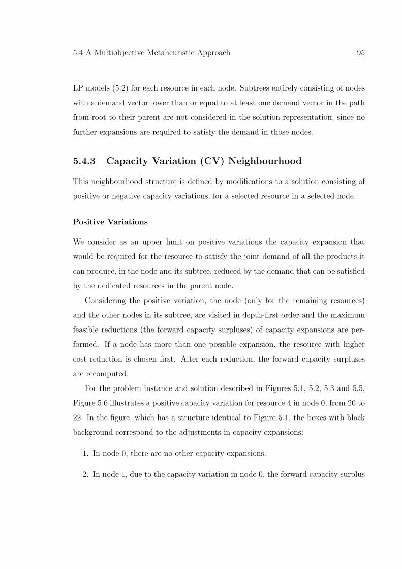
5.4 A Multiobjective Metaheuristic Approach 95
LP models (5.2) for each resource in each node. Subtrees entirely consisting of nodes
with a demand vector lower than or equal to at least one demand vector in the path
from root to their parent are not considered in the solution representation, since no
further expansions are required to satisfy the demand in those nodes.
5.4.3 Capacity Variation (CV) Neighbourhood
This neighbourhood structure is defined by modifications to a solution consisting of
positive or negative capacity variations, for a selected resource in a selected node.
Positive Variations
We consider as an upper limit on positive variations the capacity expansion that
would be required for the resource to satisfy the joint demand of all the products it
can produce, in the node and its subtree, reduced by the demand that can be satisfied
by the dedicated resources in the parent node.
Considering the positive variation, the node (only for the remaining resources)
and the other nodes in its subtree, are visited in depth-first order and the maximum
feasible reductions (the forward capacity surpluses) of capacity expansions are per-
formed. If a node has more than one possible expansion, the resource with higher
cost reduction is chosen first. After each reduction, the forward capacity surpluses
are recomputed.
For the problem instance and solution described in Figures 5.1, 5.2, 5.3 and 5.5,
Figure 5.6 illustrates a positive capacity variation for resource 4 in node 0, from 20 to
22. In the figure, which has a structure identical to Figure 5.1, the boxes with black
background correspond to the adjustments in capacity expansions:
1. In node 0, there are no other capacity expansions.
2. In node 1, due to the capacity variation in node 0, the forward capacity surplus

96 A MOMH for Mean-Risk Capacity Investment with Process Flexibility
t=0 t=1 t=2
0.5
0.5
0.25
0.25
0.25
0.25
≥≥≥≥
0
0
0
0
0
0+
0
0
0+ =
0
0
0
0
0
0
0
0
0
0
0
0
0
0
0
0
0
0
0
0
0
0
0
0
0
0
0
2
0
0
2
3
0
0
3
0
2
3
0
0
0
0
0
0
5
0
0
5
0
0
5
0
0
0
0
6
0
0
6
0
0
6
0
0
1
2
3
5
6
4
1022 822
120 1022
130 822
120 1022
150 722
160 622
≥≥≥≥ ++ =
≥≥≥≥ ++ =
≥≥≥≥ ++ =
≥≥≥≥ ++ =
≥≥≥≥ ++ =
1
0
0
1
3
0
0
3
0
1
3
0
140 822
≥≥≥≥ ++ =
Figure 5.6: Solution after positive capacity variation
for resource 3 changes to 4. The capacity expansion has a value of 4, not higher
than the capacity surplus, so it can be discarded.
3. In node 2, due to the capacity variations in nodes 0 and 1, the forward capacity
surpluses for resources 1 and 2 change to 2 and 3, respectively. The higher cost
reduction is achieved for resource 2, so its capacity expansion is reduced by 3,
to 3.
4. In node 3, due to the capacity variations in nodes 0 and 1, the forward capacity
surpluses for both resources 1 and 2 change to 2. The cost reductions are
identical, so the capacity expansion in resource 1 is reduced by 2, to 1.
5. In node 4, due to the capacity variation in node 0, the forward capacity surplus
for resource 1 changes to 3, so the entire expansion is discarded.

5.4 A Multiobjective Metaheuristic Approach 97
6. In node 5, due to the capacity variations in nodes 0 and 4, the forward capacity
surplus for resource 3 changes to 1, so its capacity expansion is reduced by 1,
to 5.
7. In node 6, due to the capacity variations in nodes 0 and 4, the forward capacity
surplus for resource 2 changes to 1, so its capacity expansion is reduced by 1,
to 6.
Negative Variations
Negative variations are limited by the backward capacity surpluses. The capacity
level has to be adjusted for the set of nodes in the path from the selected node to
the root where the selected resource’s capacity level is higher or equal to the reduced
value: in the topmost of these nodes, the resource’s expansion is reduced so that
its capacity becomes equal to the reduced value; in the remaining nodes, existing
expansions of the selected resource are discarded.
In the children of the nodes in this set that are not themselves part of the set,
expansions covering the capacity reduction in the parent node are created for the
capacity equivalent that provides them at the minimum cost. The set of expansions
for a capacity equivalent is found by, first, expanding the capacity of all its resources
by the minimum amount that covers the capacity reduction (obtained with the appli-
cation of the relevant out-shift factor), and then, iteratively reducing the expansions
as much as possible starting with the ones that present higher cost reductions.
For the problem instance and solution described in Figures 5.1, 5.2, 5.3 and 5.5,
Figure 5.7 illustrates a negative capacity variation for resource 4 in node 2, from 20
to 18. In the figure, which has a structure identical to Figure 5.1, the boxes with
black background correspond to the adjustments in capacity expansions:
1. The capacity reduction for resource 4 in node 2 is limited by its backward

98 A MOMH for Mean-Risk Capacity Investment with Process Flexibility
t=0 t=1 t=2
0.5
0.5
0.25
0.25
0.25
0.25
≥≥≥≥
0
0
0
0
0
0+
0
0
0+ =
0
0
0
0
0
4
0
0
4
0
0
0
0
0
4
3
0
0
3
0
0
0
0
0
3
0
0
2
0
4
2
6
0
0
3
0
2
6
4
3
0
0
0
0
6
0
0
6
3
0
6
3
0
0
0
7
0
0
7
0
3
7
0
0
1
2
3
5
6
4
1018 818
80 1018
100 818
80 1018
120 618
130 518
≥≥≥≥ ++ =
≥≥≥≥ ++ =
≥≥≥≥ ++ =
≥≥≥≥ ++ =
≥≥≥≥ ++ =
0
0
4
0
4
0
0
4
0
0
4
4
110 718
≥≥≥≥ ++ =
Figure 5.7: Solution after negative capacity variation
capacity surplus, with a value of 2. The capacity can not, therefore, be reduced
below 18. The proposed reduction is within this range.
2. In node 1, no changes occur since there are no expansions and capacity is not
lower than 18.
3. In node 3, an adjustment of capacity may be required, due to the capacity
reduction in its parent node. The candidates for this adjustment are the capacity
equivalents of resource 4:
• For {1, 2}, the expansions in both resources are increased by 2, and could
then be reduced by 5. Both reductions have the same cost, so the expansion
in resource 1 is discarded and the expansion in resource 2 is increased by
1, to 4.

5.4 A Multiobjective Metaheuristic Approach 99
• For {3}, the expansion is increased by 2, and could be reduced by 2.
• For {4}, the expansion is increased by 2, and could be reduced by 2.
The changes in capacity equivalent {1, 2} have the lower cost (negative, in this
case), so they are performed.
4. In node 0, the capacity expansion of resource 4 is reduced from 20 to 18.
5. In node 4, an adjustment of capacity may be required, due to the capacity
reduction in its parent node. The candidates for this adjustment are, again, the
capacity equivalents of resource 4:
• For {1, 2}, the expansions in resources 1 and 2 are both increased by 2,
and could then be reduced by 4 and 2, respectively. The achievable cost
reduction is higher for resource 2, so the expansion in resource 2 remains
0, and the expansion in resource 1 remains 3.
• For {3}, the capacity is increased by 2, and could be reduced by 2.
• For {4}, the capacity is increased by 2, and could be reduced by 2.
All alternatives lead to no changes in the expansions in this node.
5.4.4 Expansion Shift (ES) Neighbourhood
This neighbourhood structure is defined by modifications to a solution consisting of
capacity expansion cuts and partial or total shifts of capacity expansions in the same
node:
• Cut - Expansions are reduced by the selected resource’s forward capacity sur-
plus.

100 A MOMH for Mean-Risk Capacity Investment with Process Flexibility
• Same - As in negative variations, expansions covering the new capacity re-
quirements are created for the capacity equivalent that provides them at the
minimum cost, with the exception of the origin resource. The set of expansions
for a capacity equivalent is found with the same logic as in negative variations.
5.4.5 Initial Solutions
Solutions are constructed by performing a depth first traversal of the tree. At each
node, a sequence of capacity expansions are performed for a random sequence of the
products. This sequence of expansions is computed with the use of the LP models
(5.2) for the resources in the node:
• Initial conditions for all models are no demand and disabling of all capacity
utilization.
• At each iteration of the sequence of products:
– The demand for that product is introduced in the LP models, and capacity
utilization for that product is enabled.
– For each resource that is able to produce the product, the LP model is
solved in order to determine its minimum required expansion. The expan-
sion with lower cost is performed.
The last tree level at which capacity expansions can occur can be taken as a parameter,
so that for the nodes above that level, expansions will cover the node’s demand, and
for the nodes at that level, the maximum demands for each product in the node’s
subtree will have to be satisfied. This allows for some flexibility in the definition of
the timing of capacity expansion.

5.5 Computational Study 101
5.4.6 Objective Functions
Both expected value and CVaRα have been implemented. A value of α = 0.9 has
been considered.
5.5 Computational Study
5.5.1 Instances
A set of problem instances was generated for the purpose of this computational study.
The guidelines for the creation of these instances are from the work described by
Ahmed et al. (2003), Huang and Ahmed (2005) and Claro and Sousa (2007) (Ta-
ble 5.1). Straightforward adaptations were made to include the demands for 2 prod-
ucts, that were considered to be independent, and to define the amount of product
produced by unit of capacity, for which values of either 0 or 1 were considered. In
the root node, the variable costs for flexible resources are forced to be higher than
the variable costs for dedicated resources and lower than the sums of variable costs
for dedicated resources. A total of 10 instances were created, 5 for each number of
periods.
For the instances with 4 time periods, an ε-constraint method was used to obtain
the nondominated sets. For the instances with 5 time periods, the single objective
constrained problems that are solved in the ε-constraint method became very hard to
solve, requiring computational times in the order of thousands of seconds just to find
a feasible solution. Our option was, in this case, to use weighted sum formulations
of the bi-objective problem to obtain reasonable approximations to the efficient sets.
These formulations are computationally less demanding; however, they are unable to
find nonsupported efficient solutions and even some supported efficient solutions may
be missed if the intervals between the weights considered in each problem are not

102 A MOMH for Mean-Risk Capacity Investment with Process Flexibility
Table 5.1: Instance parameters
Parameter ValueBranches for nonleaf nodes 3Periods 4 (27 scenarios, 40 nodes)
5 (81 scenarios, 121 nodes)Products 2Resources 2 flexible and 2 dedicated (1 for each product)Capacity increments Integer and uniform, between 1 and 5Capacity utilization 1 for all feasible product-resource pairsDemands for root node, in t = 0 (d0) Integer and uniform, between 5 and 10
IndependentFixed costs for root node, in t = 0 (αi,0) Integer and uniform, between 2 and 10Variable costs for root node, in t = 0 (βi,0) Integer and uniform, between 1 and 5Demand and costs for a node in t > 0 Root value multiplied by lognormal variable
δ ∼ LN (µ = 1 + 0, 5t, σ = 0.5 + 0.1t)Rounded to nearest integerMinimum of 1 for fixed and variable costs
tight enough. Range equalisation was not used because the expected value and the
CVaRα have values in the same order of magnitude. A step of 0.05 was used for the
weights and a time limit of 1000 seconds was imposed for each problem. The ILOG
CPLEX 10.1 MIP solver was used.
All experiments were performed in a platform with an Intel Xeon Dual Core 5160
3.0 GHz CPU, 8 GB RAM, running Red Hat Enterprise Linux 4. The software was
generated with GCC 3.4.6 with level 3 optimisation.
Trees were implemented with tree.hh, an STL-like container class for n-ary trees,
templated over the data stored at the nodes, developed by Kasper Peeters, and avail-
able at http://www.damtp.cam.ac.uk/user/kp229/tree/. The LP problems are
solved with the ILOG CPLEX 10.1 LP solver.
The reference sets obtained with the MIP solver were used to evaluate the quality
of the approximations. For this evaluation we have chosen one of the unary quality in-
dicators with fewer limitations: the hypervolume (Zitzler and Thiele, 1998) bounded
by the set (z1, z2, ...) and a reference point (zref ) (Figure 5.8). For each instance, a
reference point has been chosen so that all points in the reference and approxima-

5.5 Computational Study 103
z1
z2
z1
z2
z3
zref
Figure 5.8: Hypervolume indicator
tion sets lie in the hypervolume, by considering the worst values for each objective
function degraded by an additional 0.1%. A relative measure was built upon this
one, consisting of the ratio between the values of the indicators for the approximation
set and the reference set, so as to enable comparison of performance across multiple
instances. The quality gap indicator being used consists of the difference to 1 of this
measure.
Considering, for example, the reference set {(1, 3) , (2, 2) , (3, 1)} and an approxi-
mation set {(2, 4) , (3, 3) , (4, 2)}, for a problem with two minimisation objectives:
• the reference point is (4.004, 4.004);
• the hypervolume of the reference set (shaded area in Figure 5.8) is 6.024016;
• the hypervolume of the approximation set is 1.016016;
• the quality gap indicator for the approximation set is 1− 1.016016/6.024016 =
83.13%.
5.5.2 Algorithm Configuration
These computational experiments have been performed with an adaptation of TA-
MOCO, as implemented in MetHOOD, with no tabu list and with fixed or variable
sub-neighbourhoods. These configurations can be viewed as a Multiobjective Random
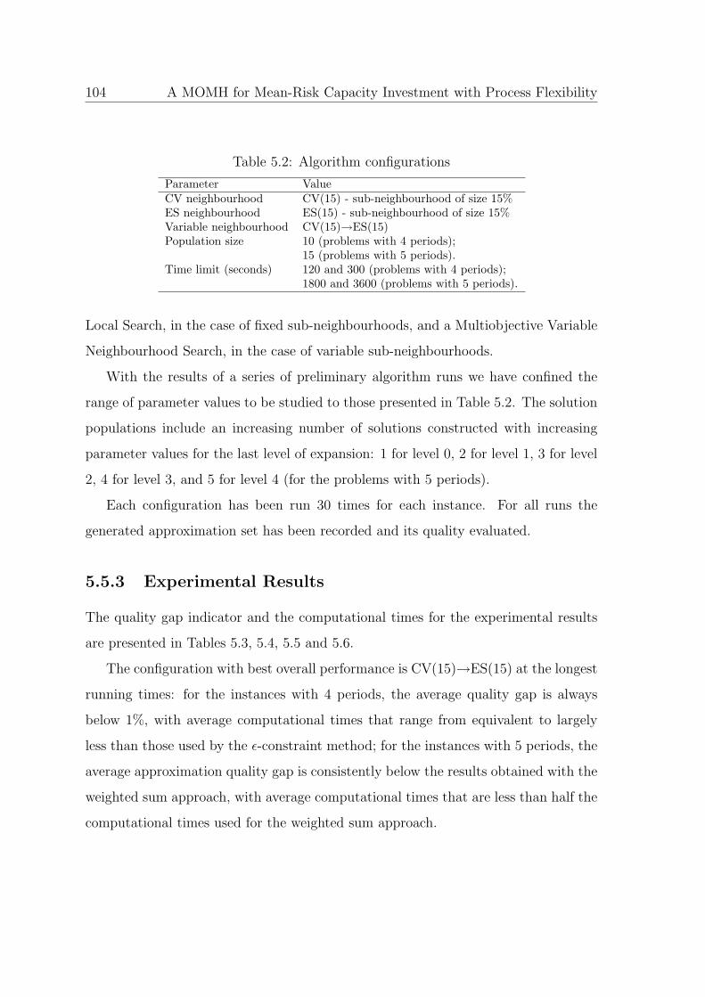
104 A MOMH for Mean-Risk Capacity Investment with Process Flexibility
Table 5.2: Algorithm configurations
Parameter ValueCV neighbourhood CV(15) - sub-neighbourhood of size 15%ES neighbourhood ES(15) - sub-neighbourhood of size 15%Variable neighbourhood CV(15)→ES(15)Population size 10 (problems with 4 periods);
15 (problems with 5 periods).Time limit (seconds) 120 and 300 (problems with 4 periods);
1800 and 3600 (problems with 5 periods).
Local Search, in the case of fixed sub-neighbourhoods, and a Multiobjective Variable
Neighbourhood Search, in the case of variable sub-neighbourhoods.
With the results of a series of preliminary algorithm runs we have confined the
range of parameter values to be studied to those presented in Table 5.2. The solution
populations include an increasing number of solutions constructed with increasing
parameter values for the last level of expansion: 1 for level 0, 2 for level 1, 3 for level
2, 4 for level 3, and 5 for level 4 (for the problems with 5 periods).
Each configuration has been run 30 times for each instance. For all runs the
generated approximation set has been recorded and its quality evaluated.
5.5.3 Experimental Results
The quality gap indicator and the computational times for the experimental results
are presented in Tables 5.3, 5.4, 5.5 and 5.6.
The configuration with best overall performance is CV(15)→ES(15) at the longest
running times: for the instances with 4 periods, the average quality gap is always
below 1%, with average computational times that range from equivalent to largely
less than those used by the ε-constraint method; for the instances with 5 periods, the
average approximation quality gap is consistently below the results obtained with the
weighted sum approach, with average computational times that are less than half the
computational times used for the weighted sum approach.

5.5 Computational Study 105
Table 5.3: Computational study for instances with 4 periods and time limit 300 s
Quality Gap(%) Time (seconds)CV(15) CV(15)→ES(15) CV(15) CV(15)→ES(15)
Instance Mean St. Dev. Mean St. Dev. Mean St. Dev. Mean St. Dev. ε-constraint4 1 0.40 0.39 0.38 0.40 236.91 61.37 212.43 58.30 642.814 2 0.56 0.55 0.65 0.56 199.42 81.39 195.30 76.67 675.694 3 0.00 0.00 0.00 0.00 74.88 45.99 34.38 22.34 59329.684 4 1.04 0.00 0.98 0.18 59.48 35.82 88.07 63.07 1773.564 5 0.18 0.14 0.15 0.13 101.04 78.88 133.82 83.99 129.28
Table 5.4: Computational study for instances with 4 periods and neighbourhoodCV(15)→ES(15)
Quality Gap(%) Time (seconds)120 s 300 s 120 s 300 s
Instance Mean St. Dev. Mean St. Dev. Mean St. Dev. Mean St. Dev. ε-constraint4 1 0.98 0.53 0.38 0.40 95.48 20.50 212.43 58.30 642.814 2 1.05 0.63 0.65 0.56 72.29 26.33 195.30 76.67 675.694 3 0.00 0.00 0.00 0.00 41.22 26.04 34.38 22.34 59329.684 4 1.08 0.14 0.98 0.18 61.37 31.30 88.07 63.07 1773.564 5 0.28 0.10 0.15 0.13 52.63 37.16 133.82 83.99 129.28
Two statistical comparisons between algorithm configurations were performed: for
the variable neighbourhood configuration, between shorter and longer running times;
for the longer running times, between single and variable neighbourhood configura-
tions. These comparisons were performed separately for the group of instances with
4 time periods and the group of instances with 5 time periods. The data violates
ANOVA assumptions, so pairwise comparisons of the algorithms were performed for
each instance, using Mann-Whitney tests, and the individual significance levels were
adjusted using a Bonferroni correction to provide an overall significance level of 0.05.
For each group of 5 instances, 10 comparisons were performed, resulting in an indi-
vidual significance level of 0.005.
Comparing the single and variable neighbourhood configurations, with longer run-
ning times, statistically significant differences in approximation quality were found
for only one instance with 5 periods. No other significant differences were found.
In the group of instances with 4 periods, the increase in available running time
resulted in statistically significant improvements for 3 instances. For the remaining

106 A MOMH for Mean-Risk Capacity Investment with Process Flexibility
Table 5.5: Computational study for instances with 5 periods and time limit 3600 s
Quality Gap(%) Time (seconds)CV(15) CV(15)→ES(15) CV(15) CV(15)→ES(15)
Instance Mean St. Dev. Mean St. Dev. Mean St. Dev. Mean St. Dev. Weighted Sum5 1 -4.17 0.52 -4.34 0.45 3182.35 446.22 3302.17 366.65 6987.275 2 0.19 0.70 -0.97 0.59 3512.45 158.89 3479.32 171.02 13424.905 3 -0.74 1.85 -1.19 1.47 2953.42 644.63 3111.35 492.69 6635.445 4 -11.53 3.96 -13.38 2.66 2694.72 771.68 2905.17 722.74 11190.905 5 -3.94 1.93 -4.69 1.26 2786.22 669.36 3082.48 547.46 9523.72
Table 5.6: Computational study for instances with 5 periods and neighbourhoodCV(15)→ES(15)
Quality Gap(%) Time (seconds)1800 s 3600 s 1800 s 3600 s
Instance Mean St. Dev. Mean St. Dev. Mean St. Dev. Mean St. Dev. Weighted Sum5 1 -3.57 0.85 -4.34 0.45 1730.49 86.48 3302.17 366.65 6987.275 2 0.27 1.14 -0.97 0.59 1792.11 34.31 3479.32 171.02 13424.905 3 0.15 1.55 -1.19 1.47 1669.71 177.87 3111.35 492.69 6635.445 4 -12.51 3.11 -13.38 2.66 1483.94 268.58 2905.17 722.74 11190.905 5 -4.08 1.56 -4.69 1.26 1709.30 193.76 3082.48 547.46 9523.72
instances (4 3 and 4 4) an early convergence, as can be observed by the similarity
in convergence times, justifies the absence of differences. In the group of instances
with 5 periods, the increase in available computational time resulted in statistically
significant improvements also for 3 instances. For the remaining instances (5 4 and
5 5) a large dispersion of the results renders the quality improvement statistically
insignificant.
5.6 Conclusions
Our previous work (Claro and Sousa, 2007) went beyond work reported in the lit-
erature regarding multistage capacity expansion under uncertainty, by presenting an
approach that considered lumpiness in capacity and both mean and risk criteria. Here
we have extended that work here by considering process flexibility in the resources.
The resulting problem is a MIP problem that we have addressed with a multiobjective
local search metaheuristic, integrating linear programming to tackle the continuous

5.6 Conclusions 107
decisions on the utilization of the available flexible capacity to satisfy demand.
MIP solvers can be used to obtain efficient sets for this problem, for example
using the ε-constraint method. The computational times, however, soon become
prohibitive, whereas the approach presented here leads to high quality approximations
to the efficient sets in comparatively reduced computational times.
The incorporation of flexible capacity is a first step to enrich this capacity ex-
pansion model. In future work we will be aiming at incorporating product prices,
processing costs and capacity leadtimes in the model. Another line of development
that we will be looking into is the integration of this optimisation model with a
game-theoretic framework to tackle capacity expansion in multiresource multiagent
networks.

108 A MOMH for Mean-Risk Capacity Investment with Process Flexibility

Chapter 6
Conclusion
6.1 Background
Many important decisions in Operations Management, in particular at a strategic
level, are made in the presence of uncertainty, and should naturally consider the
variability of their results. However, the majority of research and applied work in
this area ignores this aspect and focuses exclusively on an expected value decision
criterion. These decision settings are usually complex and if mathematical models
are to be used to characterise them, they are required to include uncertainty in the
parameters, logical and other discrete decision variables, and multiple objectives.
One of the critical decision areas within Operations Strategy is Capacity Expan-
sion, which is concerned with deciding the type, magnitude, timing, and location of
capacity acquisition. Capacity models are required to address a variety of problem
features related to the previously mentioned complexity, leading to nonlinearities,
nonconvexities, integrality and multiple objectives.
Multiobjective metaheuristics are optimisation algorithms extremely well suited
to efficiently tackle problems that present these difficulties and have therefore the
potential to play an important role as general approaches for mean-risk combina-
109

110 Conclusion
torial optimisation problems. The primary objective of our work was to perform a
preliminary assessment of this potential.
6.2 Main Contributions
Static Stochastic Knapsack
We have proposed an approach that:
• is able to handle both exact and sample approximation formulations of the
problem, and extends these formulations to consider both mean and risk criteria;
• produces high quality approximations to the efficient sets in computational
times much shorter than state-of-the-art IP and QIP/QCIP solvers;
• can easily accommodate different risk measures by simply changing the imple-
mentation of the corresponding objective function.
Multistage Capacity Investment
The approach developed for this problem:
• extends previous formulations proposed in the literature, by considering lumpi-
ness in capacity expansions and both mean and risk criteria;
• produces high quality approximations to the efficient sets in computational
times much shorter than state-of-the-art IP solvers.
Multistage Capacity Investment with Process Flexibility
We have developed an approach for this problem that:

6.3 Future Developments 111
• extends our previous formulation by considering process flexibility in the re-
sources;
• addresses the continuous decisions in a MIP problem integrating linear pro-
gramming in a multiobjective local search metaheuristic;
• can obtain high quality approximations to the efficient sets in comparatively
reduced computational times.
General Contributions
In a more general perspective, we can view the main contributions of the work pre-
sented in this dissertation as being the following:
• we explicitly introduce a multiobjective mean-risk framework for the general
class of Stochastic Combinatorial Optimisation problems;
• we propose and assess the potential of multiobjective metaheuristics as a class of
algorithms well suited to deal with the difficulties presented by these problems.
6.3 Future Developments
In the broader scope of decision making in Operations Strategy, Capacity Expansion
problems are probably the application area where our work may have a larger impact.
In a near future, the developments of this work should focus on:
• the enrichment of the capacity expansion model, incorporating product prices,
processing costs and capacity leadtimes;
• integrating the multiobjective optimisation framework with a game-theoretic
framework to tackle multiresource multiagent networks, this being a natural

112 Conclusion
extension of capacity investment models since capacity decisions often are con-
tingent upon the decisions of the other economic agents (customers, suppliers,
partners, competitors) in the network.
Alongside these developments, two additional research topics, of a more practical
nature, should be considered:
• one is the task of deriving managerial insights from these models, a task that is
acknowledgedly difficult to pursue due to the complexity of the models;
• the other is the recognition of the gap between these tools and the tools that
are required in practice to support corporate decisions, and the resulting need
to set up research and development initiatives to bridge that gap.
On the other hand, concerning the application of multiobjective metaheuristics
to stochastic combinatorial optimisation problems, we intend to focus on some in-
cremental but natural developments to our work. Two possibilities of enhancing the
Multiobjective Local Search template would be worth exploring:
• one would be to accommodate specific characteristics and components of sto-
chastic problems, such as scenario trees or objective functions that are computed
from a common vector of objective function values for each scenario;
• the other would be to generalise and incorporate the algorithmic solutions that
have typically been used to adapt single-objective metaheuristics to stochastic
optimisation - the incorporation of sampling methods for solution evaluation,
and statistical inference methods for solution comparison.

Bibliography
Ahmed, M. A. and Alkhamis, T. M. (2002). Simulation-based optimization using
simulated annealing with ranking and selection. Comput. Oper. Res., 29(4):387–402.
Ahmed, S. (2006). Convexity and decomposition of mean-risk stochastic programs.
Math. Program., 106(3):433–446.
Ahmed, S., King, A., and Parija, G. (2003). A multi-stage stochastic integer pro-
gramming approach for capacity expansion under uncertainty. J. Global Optim.,
26(1):3–24.
Ahmed, S. and Sahinidis, N. V. (2003). An approximation scheme for stochastic
integer programs arising in capacity expansion. Oper. Res., 51(3):461–471.
Alrefaei, M. H. and Andradottir, S. (1999). A simulated annealing algorithm with
constant temperature for discrete stochastic optimization. Manag. Sci., 45(5):748–
764.
Artzner, P., Delbaen, F., Eber, J. M., and Heath, D. (1999). Coherent measures of
risk. Math. Finance, 9(3):203–228.
Battiti, R. and Tecchiolli, G. (1992). Parallel biased search for combinatorial opti-
mization - genetic algorithms and TABU. Microproc. Microsyst., 16(7):351–367.
113

114 Bibliography
Beach, R., Muhlemann, A. P., Price, D. H. R., Paterson, A., and Sharp, J. A. (2000).
Manufacturing operations and strategic flexibility: survey and cases. Int. J. Oper.
Prod. Manag., 20(1):7–30.
Bean, J. C., Higle, J. L., and Smith, R. L. (1992). Capacity expansion under sto-
chastic demands. Oper. Res., 40(S2):210–216.
Berman, O., Ganz, Z., and Wagner, J. M. (1994). A stochastic optimization model
for planning capacity expansion in a service industry under uncertain demand. Nav.
Res. Log., 41(4):545–564.
Carraway, R. L., Schmidt, R. L., and Weatherford, L. R. (1993). An algorithm
for maximizing target achievement in the stochastic knapsack-problem with normal
returns. Nav. Res. Log., 40(2):161–173.
Chang, T. J., Meade, N., Beasley, J. E., and Sharaiha, Y. M. (2000). Heuristics for
cardinality constrained portfolio optimisation. Comput. Oper. Res., 27(13):1271–
1302.
Chen, Z.-L., Li, S., and Tirupati, D. (2002). A scenario-based stochastic pro-
gramming approach for technology and capacity planning. Comput. Oper. Res.,
29(7):781–806.
Cheng, L., Subrahmanian, E., and Westerberg, A. W. (2003). Design and planning
under uncertainty: issues on problem formulation and solution. Comput. Chem.
Eng., 27(6):781–801.
Cheng, L. F., Subrahmanian, E., and Westerberg, A. W. (2004). Multi-objective
decisions on capacity planning and production - inventory control under uncertainty.
Ind. Eng. Chem. Res., 43(9):2192–2208.

Bibliography 115
Claro, J. and Sousa, J. P. (2001). An object-oriented framework for multiobjective
local search. In Sousa, J. P., editor, MIC’2001 4th Metaheuristics Int. Conf., pages
231–236, Porto, Portugal.
Claro, J. and Sousa, J. P. (2007). A multiobjective metaheuristic for a mean-risk
multistage capacity investment problem. Submitted for publication.
Cohn, A. M. and Barnhart, C. (1998). The stochastic knapsack problem with ran-
dom weights: a heuristic approach to robust transportation planning. In Triennial
Sympos. Transportation Anal. (TRISTAN III), San Juan, Puerto Rico.
Costa, D. and Silver, E. A. (1998). Tabu search when noise is present: An illustration
in the context of cause and effect analysis. J. Heuristics, 4(1):5–23.
Crama, Y. and Schyns, M. (2003). Simulated annealing for complex portfolio selec-
tion problems. Eur. J. Oper. Res., 150(3):546–571.
Czyzak, P. and Jaszkiewicz, A. (1998). Pareto simulated annealing - a metaheuris-
tic technique for multiple-objective combinatorial optimization. J. Multi-Criteria
Decision Anal., 7(1):34–47.
Das, I. (2000). Robustness optimization for constrained nonlinear programming
problems. Eng. Optim., 32(5):585–618.
Das, S. and Ghosh, D. (2003). Binary knapsack problems with random budgets. J.
Oper. Res. Soc., 54(9):970–983.
Davis, M. H. A., Dempster, M. A. H., Sethi, S. P., and Vermes, D. (1987). Optimal
capacity expansion under uncertainty. Adv. Appl. Prob., 19(1):156–176.
de Groote, X. (1994). The flexibility of production processes: a general framework.
Manag. Sci., 40(7):933–945.

116 Bibliography
Deb, K. and Gupta, H. (2004). Introducing robustness in multiobjective optimiza-
tion. Technical Report 2004016, Kanpur Genetic Algorithms Laboratory (KanGAL),
Indian Institute of Technology, Kanpur, India.
Dixit, A. K. and Pindyck, R. S. (1994). Investment Under Uncertainty. Princeton
University Press, Princeton, NJ.
Ehrgott, M. and Gandibleux, X. (2000). A survey and annotated bibliography of
multiobjective combinatorial optimization. OR Spectrum, 22(4):425–460.
Ehrgott, M. and Gandibleux, X. (2004). Approximative solution methods for multi-
objective combinatorial optimization. TOP (Spanish journal of operations research),
12(1):1–90.
Ehrgott, M., Klamroth, K., and Schwehm, C. (2004). An MCDM approach to
portfolio optimization. Eur. J. Oper. Res., 155(3):752–770.
Eichhorn, A. and Romisch, W. (2005). Polyhedral risk measures in stochastic pro-
gramming. SIAM J. Optim., 16(1):69–95.
Eppen, G. D., Martin, R. K., and Schrage, L. (1989). A scenario approach to
capacity planning. Oper. Res., 37(4):517–527.
Ferland, J. A., Hertz, A., and Lavoie, A. (1996). An object-oriented methodology
for solving assignment-type problems with neighborhood search techniques. Oper.
Res., 44(2):347–359.
Fine, C. H. and Freund, R. M. (1990). Optimal investment in product-flexible
manufacturing capacity. Manag. Sci., 36(4):449–466.
Fink, A., Voss, S., and Woodruff, D. L. (2002). Metaheuristic class libraries. In
Glover, F. and Kochenberger, G., editors, Handbook of Metaheuristics, pages 515–
535. Kluwer.
Bibliography 117
Fishburn, P. C. (1977). Mean-risk analysis with risk associated with below-target
returns. Am. Econ. Rev., 67(2):116–26.
Fonseca, C. M. and Fleming, P. J. (1995). An overview of evolutionary algorithms
in multiobjective optimization. Evol. Comput., 3:1–16.
Freidenfelds, J. (1980). Capacity expansion when demand is a birth-death random
process. Oper. Res., 28(3):712–721.
Freville, A. (2004). The multidimensional 0-1 knapsack problem: An overview. Eur.
J. Oper. Res., 155(1):1–21.
Freville, A. and Plateau, G. (1994). An efficient preprocessing procedure for the
multidimensional 0-1-knapsack problem. Discrete Appl. Math., 49(1-3):189–212.
Gamma, E., Helm, E., Johnson, R., and Vlissides, J. (1994). Design Patterns:
Elements of Reusable Object-Oriented Software. Addison Wesley, Massachussets.
Gandibleux, X. and Freville, A. (2000). Tabu search based procedure for solving
the 0-1 multiobjective knapsack problem: The two objectives case. J. Heuristics,
6(3):361–383.
Gandibleux, X., Mezdaoui, N., and Freville, A. (1997). A multiobjective tabu search
procedure to solve combinatorial optimization problems. In Caballero, R., Ruiz, F.,
and Steuer, R., editors, Adv. Mult. Objective Goal Program., volume 445 of Lect.
Notes Econ. Math. Syst., pages 291–300. Springer.
Glover, F. (1986). Future paths for integer programming and links to artificial-
intelligence. Comput. Oper. Res., 13(5):533–549.
Gutjahr, W. J. (2003). A converging ACO algorithm for stochastic combinatorial
optimization. In Albrecht, A. and Steinhofel, K., editors, Stoch. Alg.: Found. Appl.,
volume 2827 of Lect. Notes Comput. Sci., pages 10–25. Springer.

118 Bibliography
Hanafi, S. and Freville, A. (1998). An efficient tabu search approach for the 0-1
multidimensional knapsack problem. Eur. J. Oper. Res., 106(2-3):659–675.
Hansen, M. P. (2000). Tabu search for multiobjective combinatorial optimization:
TAMOCO. Control Cybern., 29(3):799–818.
Haugen, K. K., Lokketangen, A., and Woodruff, D. L. (2001). Progressive hedging as
a meta-heuristic applied to stochastic lot-sizing. Eur. J. Oper. Res., 132(1):116–122.
Henig, M. I. (1990). Risk criteria in a stochastic knapsack-problem. Oper. Res.,
38(5):820–825.
Hill, I. D. (1973). Algorithm AS66: The normal integral. Appl. Statist., 22(3):424–
427.
Huang, K. and Ahmed, S. (2005). The value of multi-stage stochastic programming
in capacity planning under uncertainty. Submitted for publication.
Jaszkiewicz, A. (2002). On the performance of multiple-objective genetic local search
on the 0/1 knapsack problem - a comparative experiment. IEEE Trans. Evol. Com-
put., 6(4):402–412.
Jin, Y. and Branke, J. (2005). Evolutionary optimization in uncertain environments
- a survey. IEEE Trans. Evol. Comput., 9(3):303–317.
Jin, Y. C. and Sendhoff, B. (2003). Trade-off between performance and robustness:
An evolutionary multiobjective approach. In Goos, G., Hartmanis, J., and van
Leeuwen, J., editors, Evol. Multi-Criterion Optim., Proc., volume 2632 of Lect. Notes
Comput. Sci., pages 237–251. Springer.
Johnson, R. E. and Foote, B. (1988). Designing reusable classes. J. Object-Orient.
Program., 1(2):22–35.

Bibliography 119
Jones, D. F., Mirrazavi, S. K., and Tamiz, M. (2002). Multi-objective meta-
heuristics: An overview of the current state-of-the-art. Eur. J. Oper. Res., 137(1):1–
9.
Julka, N., Baines, T., Tjahjono, B., Lendermann, P., and Vitanov, V. (2007). A re-
view of multi-factor capacity expansion models for manufacturing plants: Searching
for a holistic decision aid. Int. J. Prod. Econ., 106(2):607–621.
Kleywegt, A. J., Shapiro, A., and Homem-De-Mello, T. (2002). The sample aver-
age approximation method for stochastic discrete optimization. SIAM J. Optim.,
12(2):479–502.
Kouvelis, P. (1992). Design and planning problems in flexible manufacturing systems:
a critical review. J. Intell. Manuf., 3(2):75–99.
Kristoffersen, T. K. (2005). Deviation measures in linear two-stage stochastic pro-
gramming. Math. Methods Oper. Res., 62(2):255–274.
Li, S. and Tirupati, D. (1994). Dynamic capacity expansion problem with multi-
ple products: Technology selection and timing of capacity additions. Oper. Res.,
42(5):958–976.
Liu, M. and Sahinidis, N. (1996). Optimization in process planning under uncer-
tainty. Ind. Eng. Chem. Res., 35(11):4154–4165.
Manne, A. S. (1961). Capacity expansion and probabilistic growth. Econometrica,
29(4):632–649.
Markert, A. and Schultz, R. (2004). On deviation measures in stochastic integer
programming. Oper. Res. Letters, 33(5):441–449.

120 Bibliography
Markowitz, H. M. (1959). Portfolio selection: efficient diversification of investments.
Wiley, New York,.
Morton, D. P. and Wood, R. K. (1998). On a stochastic knapsack problem and
generalizations. In Woodruff, D. L., editor, Adv. in Comput. and Stoch. Optim.,
Logic Program., and Heuristic Search: Interfaces in Comput. Sci. and Oper. Res.,
pages 149–168. Kluwer Academic Publishers, Dordrecht, the Netherlands.
Markert, A. (2004). Deviation measures in stochastic programming with mixed-
integer recourse. PhD thesis, Institute of Mathematics, University of Duisburg-
Essen.
Nievergelt, N. (1994). Complexity, algorithms, programs, systems: the shifting focus.
J. Symb. Comput., 17(4):297–310.
Ogryczak, W. and Ruszczynski, A. (1999). From stochastic dominance to mean-risk
models: Semideviations as risk measures. Eur. J. Oper. Res., 116(1):33–50.
Ogryczak, W. and Ruszczynski, A. (2002). Dual stochastic dominance and related
mean-risk models. SIAM J. Optim., 13(1):60–78.
Phelps, S. and Koksalan, M. (2003). An interactive evolutionary metaheuristic for
multiobjective combinatorial optimization. Manag. Sci., 49(12):1726–1738.
Pirlot, M. (1996). General local search methods. Eur. J. Oper. Res., 92(3):493–511.
Rajagopalan, S., Singh, M. R., and Morton, T. E. (1998). Capacity expansion and
replacement in growing markets with uncertain technological breakthroughs. Manag.
Sci., 44(1):12–30.
Ray, T. (2002). Constrained robust optimal design using a multiobjective evolution-
ary algorithm. In Proc. 2002 Cong. Evol. Comput., 2002, CEC ’02, volume 1, pages
419–424.

Bibliography 121
Rockafellar, R. T. and Uryasev, S. (2002). Conditional value-at-risk for general loss
distributions. J. Banking Finance, 26(7):1443–1471.
Rockafellar, R. T. and Wets, R. J. B. (1991). Scenarios and policy aggregation in
optimization under uncertainty. Math. Oper. Res., 16(1):119–147.
Rosen, S. L. and Harmonosky, C. M. (2005). An improved simulated annealing
simulation optimization method for discrete parameter stochastic systems. Comput.
Oper. Res., 32(2):343–358.
Rudberg, M. and Olhager, J. (2003). Manufacturing networks and supply chains:
an operations strategy perspective. Omega, 31(1):29–39.
Ruszczynski, A. and Shapiro, A. (2006). Optimization of convex risk functions.
Math. Oper. Res., 31(3):433–452.
Sahinidis, N. V. (2004). Optimization under uncertainty: state-of-the-art and op-
portunities. Comput. Chem. Eng., 28(6-7):971–983.
Schaffer, J. D. (1985). Multiple objective optimization with vector evaluated genetic
algorithms. In Grefenstette, J. J., editor, Gen. Alg. Appl.: Proc. First Int. Conf.
Gen. Alg., pages 92–100. Lawrence Erlbaum.
Schlottmann, F. and Seese, D. (2004). A hybrid heuristic approach to discrete multi-
objective optimization of credit portfolios. Comput. Statist. Data Anal., 47(2):373–
399.
Schultz, R. (2003). Stochastic programming with integer variables. Math. Program.,
97(1-2):285–309.
Schultz, R. and Tiedemann, S. (2006). Conditional value-at-risk in stochastic pro-
grams with mixed-integer recourse. Math. Program., 105(2-3):365–386.

122 Bibliography
Serafini, P. (1992). Simulated annealing for multiple objective optimization prob-
lems. In Proc. Tenth Int. Conf. Mult. Criteria Decision Making, pages 87–96, Taipei
- Taiwan.
Sethi, A. K. and Sethi, S. P. (1990). Flexibility in manufacturing: A survey. Int. J.
Flex. Manuf. Syst., 2(4):289–328.
Shapiro, A. and Ahmed, S. (2004). On a class of minimax stochastic programs.
SIAM J. Optim., 14(4):1237–1249.
Silva, C. G., Climaco, J., and Figueira, J. (2006). A scatter search method for
bi-criteria {0,1}-knapsack problems. Eur. J. Oper. Res., 169(2):373–391.
Sniedovich, M. (1980). Preference order stochastic knapsack-problems: Methodolog-
ical issues. J. Oper. Res. Soc., 31(11):1025–1032.
Sniedovich, M. (1981). Some comments on preference order dynamic-programming
models. J. Math. Anal. Appl., 79(2):489–501.
Steinberg, E. and Parks, M. S. (1979). Preference order dynamic program for a
knapsack problem with stochastic rewards. J. Oper. Res. Soc., 30(2):141–147.
Steuer, R. E. and Na, P. (2003). Multiple criteria decision making combined with
finance: A categorized bibliographic study. Eur. J. Oper. Res., 150(3):496–515.
Swaminathan, J. M. (2000). Tool capacity planning for semiconductor fabrication
facilities under demand uncertainty. Eur. J. Oper. Res., 120(14):545–558.
Takriti, S. and Ahmed, S. (2004). On robust optimization of two-stage systems.
Math. Program., 99(1):109–126.

Bibliography 123
Teghem, J., Tuyttens, D., and Ulungu, E. L. (2000). An interactive heuristic method
for multi-objective combinatorial optimization. Comput. Oper. Res., 27(7-8):621–
634.
Tomlin, B. and Wang, Y. (2005). On the value of mix flexibility and dual sourcing
in unreliable newsvendor networks. Manuf. Serv. Oper. Manag., 7(1):37–57.
Toni, A. D. and Tonchia, S. (1998). Manufacturing flexibility: a literature review.
Int. J. Prod. Res., 36(31):1587–1617.
Ulungu, E. L., Teghem, J., Fortemps, P. H., and Tuyttens, D. (1998). MOSA
method: a tool for solving multiobjective combinatorial optimization problems. J.
Multi-Criteria Decision Anal., 8(4):221–236.
Van Mieghem, J. A. (1998). Investment strategies for flexible resources. Manag.
Sci., 44(8):1071–1078.
Van Mieghem, J. A. (2003). Capacity management,investment, and hedging: Review
and recent developments. Manuf. Serv. Oper. Manag., 5(4):269–302.
Van Mieghem, J. A. (2006). Risk mitigation in newsvendor networks: Resource
diversification, flexibility, sharing, and hedging. To appear in Manag. Sci.
Voss, S. and Woodruff, D. L., editors (2002). Optimization Software Class Libraries.
Kluwer, Boston.
Wheelwright, S. C. (1978). Reflecting corporate strategy in manufacturing decisions.
Bus. Horiz., 21(1):57–66.
Wichura, M. J. (1988). Algorithm AS241: The percentage points of the normal
distribution. Appl. Statist., 37(3):477–484.

124 Bibliography
Wu, S. D., Erkoc, M., and Karabuk, S. (2005). Managing capacity in the high-tech
industry: A review of literature. Eng. Econ., 50(2):125–158.
Yitzhaki, S. (1982). Stochastic dominance, mean variance, and Gini’s mean differ-
ence. Am. Econ. Rev., 72(1):178–85.
Zitzler, E. and Thiele, L. (1998). Multiobjective optimization using evolutionary
algorithms - a comparative case study. In Eiben, A. E., Back, T., Schoenauer,
M., and Schwefel, H. P., editors, Parallel Problem Solving from Nature - PPSN V,
volume 1498 of Lect. Notes Comput. Sci., pages 292–301. Springer.
Top Related