Multimodal Blending for High-Accuracy Instance Recognition

Ziang Xie, Arjun Singh, Justin Uang, Karthik S. Narayan, Pieter Abbeel

Abstract— Despite the rich information provided by sensorssuch as the Microsoft Kinect in the robotic perception setting,the problem of detecting object instances remains unsolved,even in the tabletop setting, where segmentation is greatlysimplified. Existing object detection systems often focus ontextured objects, for which local feature descriptors can be usedto reliably obtain correspondences between different views ofthe same object.

We examine the benefits of dense feature extraction andmultimodal features for improving the accuracy and robustnessof an instance recognition system. By combining multiplemodalities and blending their scores through an ensemble-based method in order to generate our final object hypotheses,we obtain significant improvements over previously publishedresults on two RGB-D datasets. On the Challenge dataset, ourmethod results in only one missed detection (achieving 100%precision and 99.77% recall). On the Willow dataset, we alsomake significant gains on the prior state of the art (achieving98.28% precision and 87.78% recall), resulting in an increasein F-score from 0.8092 to 0.9273.

I. INTRODUCTION

Object recognition remains a challenging problem incomputer vision. Researchers often divide the recognitiontask into (1) category-level recognition, where objects in aparticular category are given the same label (e.g. “bowl” or“soda can”), and (2) instance recognition, where each specificobject is given its own label (e.g. “Coke can” or “Diet Cokecan”). Several differences distinguish the robotic setting fromthe classic computer vision setting of detecting objects in 2Dimages. First, since robots in fixed environments may onlyhave to interact with on the order of hundreds of objects,instance recognition may be sufficient for a wide variety oftasks. Second, in order for robots to be able to manipulate therecognized objects, the object poses must also be determined.Finally, given the relatively low cost of RGB-D sensors, suchas the Microsoft Kinect, in comparison to other componentsof robotic platforms, both color images and point cloudsare becoming standard in the robotic perception setting [1].Despite the additional information provided by the depthchannel, no instance recognition systems are robust enoughto detect all objects in the standard benchmark settings weconsider here, let alone in highly unstructured household andoffice environments.

In this paper, we present a system which significantlyimproves on the state of the art for the above task. While we

Department of Electrical Engineering and Computer Sciences, Univer-sity of California, Berkeley, Berkeley, CA, USA. zxie@berkeley.edu,{arjun, karthik.narayan}@eecs.berkeley.edu,justin.uang@berkeley.edu, pabbeel@cs.berkeley.edu

Fig. 1: Example detection. Despite clutter and heavy occlu-sions, our approach accurately captures object class and pose.

briefly describe our end-to-end pipeline, we emphasize thatour primary contributions are as follows:1. We present experiments demonstrating that dense feature

extraction (with moderate downsampling) results in sig-nificantly higher recall than feature extraction at keypoint-based interest points. This holds at training time, whenbuilding feature models, and at test time, when extractingfeatures from the test images.

2. We illustrate how a discriminative extension of featureweighted linear stacking [2] can be used to generate objecthypotheses using a learned combination of scores derivedfrom texture, color, and shape-based features, leading toanother significant boost in performance.

3. Finally, we achieve state-of-the-art results on two in-stance recognition datasets. On the Challenge dataset,our method results in near perfect performance, (1.000precision and 0.9977 recall). On the Willow dataset, wepresent a significant leap over the previous state of the art,with .9828 precision and 0.8778 recall, corresponding toan increase in F-score from 0.8092 to 0.9273.

II. RELATED WORK

Many existing approaches toward instance recognition firstextract descriptors from a training set of objects, then matchthem to corresponding descriptors in a given test scene,using the correspondences to simultaneously determine thecorrect object and pose. One such example is the MOPEDsystem of Collet et al. [3], which first constructs a sparsedescriptor database by extracting SIFT features [4] at trainingtime. At test time, MOPED uses the SIFT features to jointlyestimate object class and pose. Unlike our system, it does not

use depth information or perform multimodal verification.Aldoma et al. [5] obtain good performance by combiningtwo pipelines, one using 2D and the other 3D features, via anoptimization-based hypothesis verification framework. Theytoo use features extracted at keypoints, and differ in their useof a 3D histogram-based feature.

While methods using the depth modality typically extractfeatures from depth maps for use in recognition, such asextensions of histograms of oriented gradients (HOG) [6],[7], spin images [8], and point feature histograms [9], weuse depth primarily for segmentation and to determine the3D correspondences of pixels in test images.

Several works on category recognition suggest that densesampling tends to yield higher performance [10], [11]. Forexample, Tuytelaars et al. [10] attribute part of the suc-cess of their Naive Bayes Nearest Neighbor classifier todense descriptor computation. In the unsupervised featurelearning context, Coates et al. [11] demonstrate that denseconvolution in convolutional neural networks leads to higherperformance. Nowak et al. also illustrate the importance ofdense sampling for bag-of-features image classification [12].To the best of our knowledge, however, this paper is thefirst to demonstrate that dense features play a crucial rolein attaining strong performance on the instance recognitionproblem.

In addition to improving performance using dense features,we consider using an ensemble of models over severalmodalities to aid in recognition. Ensemble learning, alsoreferred to as blending, has been explored thoroughly inthe machine learning community [13], [14]. One simplemethod is to learn an affine combination of the scoresobtained through each modality. Another method that extendsthis idea is feature weighted linear stacking [15], [16].We evaluate both methods for the purpose of generatinghypothesis detections.

Thorough experimentation illustrates that our approachobtains significantly better results than previous state of theart. Before presenting our approach, we first give an overviewof the test datasets, which we use as the primary evaluationmetrics.

III. PROBLEM SETTING

We evaluate our approach on two datasets, Challenge andWillow, which were collected for the 2011 ICRA Solutions inPerception Challenge. Both datasets share a set of 35 trainingobjects, which must be detected in a variety of tabletopscenes.

The training data consists of 37 views of each trainingobject, with each view containing a registered point cloudC, a 1024×1280 image I , the training object’s image mask,and the associated camera matrix K for that view. At a highlevel, we build models of each object by merging informationfrom each view. We present details of this training procedurein Section V.

The test data consists of a series of test scenes. Each testscene provides at most 20 scene views, each accompaniedby a color image I and an associated point cloud C from a

Kinect sensor. We also assume a gravity vector, which wecompute using a single scene from both the Challenge andWillow test sets, since the sensor remains fixed throughout.Test scenes can be highly cluttered, potentially containingany subset of the 35 objects in any pose, as well as imposterobjects not among the training objects. At test time, givena view with C, I , we are asked to jointly recognize eachtraining object and its pose in each view independently,while ignoring imposter objects. The datasets differ greatlyin difficulty; the Challenge dataset consists of 39 test sceneswhich may each contain multiple objects with low occlusionsand no imposter objects, while the Willow dataset consistsof 24 test scenes with heavy (possibly even full) occlusionsas well as imposter objects. We present sample training andtesting data from each dataset in Section 5.

Our current solution operates under the following assump-tions, satisfied by both the Willow and Challenge datasets:1. Training objects have relatively non-specular and non-

transparent surfaces; RGB-D sensors using structured-light approaches (e.g. the Kinect) can, at best, generatenoisy, incomplete point clouds of highly-specular or trans-parent objects.

2. Training objects contain texture: we use gradient-baseddescriptors to estimate training object poses.

3. Objects in test scenes are supported by a tabletop plane:this allows for simple test scene segmentation (Section V).From here, we organize the paper as follows: we first

present a brief overview of our system, which builds on Tanget al. [17]. We then present our main contributions, namelyan examination of dense feature extraction, multimodal fea-ture models and pose-based verification, and multimodalblending. Finally, we conclude with a series of experimentsdetailing the performance of our pipeline on the Challengeand Willow datasets.

IV. SYSTEM OVERVIEW

At training time, we first merge point clouds from multipleviews of each training object, then construct a mesh usingPoisson reconstruction. After extracting features from imagesof each view of the object, we then project the features ontothe mesh. The resulting descriptor list with associated 3Dmodel coordinates constitutes a feature model. Section V-Adetails our feature computation approach, and Section V-Bdetails the types of feature we use.

At test time, we first detect table planes in the scene usinga RANSAC plane fitting approach, eliminating hypothesesusing the gravity vector for the dataset and selecting the high-est supporting plane. We then apply agglomerative clusteringto points lying above this supporting plane. Next, we projecteach test cluster onto the images to form image masks andextract features from unmasked portions of the image. Toobtain the 3D coordinates associated with each feature, weproject features extracted from the masked image back ontothe 3D point cloud.

Algorithm 1 describes the procedure we run on each testcluster to compute a RANSAC score and pose estimate foreach candidate object. We then use Algorithm 2 to compute

Point Clouds

Merged Clouds

3D Mesh

Image Data

Mask Image

Extract Features

Object Model

Point Clouds

Object Clusters

Image Data

Extract Features

RANSAC + Pose Estimation

Mode1

Mode2

Mode3

Meta

SVM

Multimodal Blending

Generate Occlusion Data

Verify

Fig. 2: An overview of our pipeline. The top row shows the training pipeline, and the bottom row shows the test pipeline.

Symbol Description

I ∼ a color imagep ∼ a point (x, y, z)P ∼ a point cloud of size |P |f ∼ an image feature descriptorF ∼ a set of descriptors of size |F |M ∼ a feature model or (P, F ) pair with

each pi corresponding to fiC ∼ a set of feature correspondencesp(f) ∼ point corresponding to descriptor f

NN(f,Md) ∼ nearest neighbor of feature f in modelMd, d ∈ {shape, color, SIFT}

ε ∼ distance threshold—either in featurespace (εd) or 3D space (ε3D)

s ∼ score—either RANSAC (sNN) or ver-ification (sd)

T ∼ an estimated 6DOF poseNobj ∼ number of training objects

NRANSAC ∼ number of RANSAC iterations

TABLE I: Summary of Notation

pose-based verification scores (one for each type of feature)for each candidate object using their estimated poses.

Finally, we compute metafeatures on the test scenes(see Table II), and, given the metafeatures as well as theRANSAC and verification scores, we use a multimodalblender to output our final object hypotheses (Section V-C).

V. METHODS

We now describe the key contributions of our approach,namely dense feature extraction, pose-based verification us-

Algorithm 1: RANSAC Pose EstimationInput: test cluster P test, corresponding test features

F test, feature models {Mdi }

Nobj

i=1 where d is themodel feature type, query-to-model NNcorrespondences {Ci}Nobj

i=1

Output: RANSAC scores {sNNi }

Nobj

i=1 , estimated poses{Ti}Nobj

i=1

Initialize {sNNi = −∞}Nobj

i=1

for i = 1 to Nobj dofor j = 1 to NRANSAC do

Cij ← sample 3 correspondences from CiTij ← EstimateTransform(Cij)Align P test to Md

i using Tifor j = 1 to |P test| do

if ‖pj − p(NN(fj ,Mdi ))‖2 < ε3D then

sNNij = sNN

ij + 1 // Increment score

endendif sNN

ij > sNNi then

sNNi = sNN

ij // Update best score

Ti = Tij // Update best pose

endend

end

ing multiple feature models, and multimodal blending.

A. Dense Feature Extraction

We compute image features densely at both training andtest time. At training time, rather than keep descriptors com-puted at every pixel, we employ voxel grid downsampling(with a leaf size of 0.5cm) of the descriptors for each viewafter projecting them onto the object mesh. At test time, we

Algorithm 2: Pose-based VerificationInput: test cluster P test, corresponding test features

F test, estimated poses {Ti}Nobj

i=1 , feature models{Md

i }Nobj

i=1 , where d is the feature model typeOutput: verification scores {sdi }

Nobj

i=1

Initialize {sdi = 0}Nobj

i=1

for i = 1 to Nobj doAlign P test to Md

i using Tifor j = 1 to |P test| do

// Radius search finds all model points

// within ε3D of ptestj in Mdi when aligned

F trainij , P train

ij ← RadiusSearch(Mdi , ptestj , ε3D)

for k = 1 to |P trainij | do

if ‖f testj − f trainijk ‖2 < εd thensdi = sdi + 1 // Increment score

breakend

endend

end

use a stride of 20px for the query image descriptors. Usingthese two methods hardly impacts performance due to highcorrelation between neighboring descriptors, and still yieldsapproximately 5 to 10 times as many descriptors as usingkeypoints. See Section VI-D for a detailed analysis of theresults using keypoints versus our dense sampling approach.

As described in Algorithm 1, we attempt to align eachtraining object to a given test cluster using the SIFT featuremodel. Empirically, we find that the training object yieldingthe highest sNN usually matches the testing object, assumingthe test object is not an imposter.

In the presence of imposters and spurious segmentations,the ratio between the first and second highest sNN is areliable indicator of whether the first ranked object shouldbe declared.1 This baseline approach alone yields 100%precision and 99.31% recall on the Challenge dataset (whichcontains no imposters), but far from perfect performance onthe Willow dataset (93.82% precision and 83.97% recall).

B. Multimodal Feature Models and Pose-Based Verification

Motivated by the remaining errors on the Willow dataset,we also construct models to exploit local color and shapeinformation in addition to the models using gradient-basedimage descriptors. Concretely, we construct color featuremodels using L*a*b* values at each pixel, and shape featuremodels using shape context features computed in a similarfashion as described by Belongie et al. [18], using theadditional depth information to scale the downsampled edgepoints before binning.

After detecting and estimating the pose of an object in ascene, we then perform a verification of the detection usingeach of the SIFT, shape, and color models (Algorithm 2).

1Specifically, we use rNN = 1.5; if the ratio is lower than this thanwe do not declare a detection.

(a) Example of nontextured testobject view.

(b) Example test scene withonly two non-imposters.

Fig. 3: Cases where our multimodal approach improvesperformance.

These scores ({scolor, sSIFT, sshape}Nobj

i=1 ) provide additionalinformation for whether to declare or eliminate a detection.

Intuitively, the multimodal approach leverages the strengthof each feature type in different contexts. For example, fewtexture cues in an object view (e.g. Figure 3a) typically yieldlow RANSAC scores, rendering the ratio test unreliable.In this case, shape cues can provide information regardingcorrect object detection.

Color information also greatly helps in improving preci-sion. Given that our procedure estimates an accurate pose,the color ratio check

scolori

|F test| > rcolor

then serves as a reliable indicator of whether object i is thecorrect object. One case in particular this check works wellfor is instances of different flavors, such as the Odwallabottles shown in Figure 3b, where the algorithm cannotreliably distinguish objects using only gradient or local shapeinformation.

Given object hypotheses for a test cluster, we apply thecolor ratio check described above as well as verify that theobject hypothesis ranks at the top in at least half of the modelscores before declaring a detection.

C. Multimodal Blending

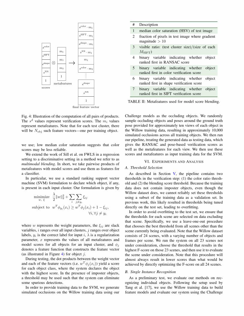
There are many rules that could be used in addition to thecolor ratio threshold described in the previous section. Ratherthan relying on (typically tedious and labor-intensive) hand-engineering to generate such rules for combining the multiplemodalities, we use a method inspired by the feature-weightedlinear stacking (FWLS) approach proposed by Sill et al. [2].This method blends the scores obtained using each modelthrough a systematic, data-driven approach. Furthermore, thismethod can leverage the intuition that certain models maybe more reliable in some settings than others.

The FWLS approach described by Sill et al. blends themodel outputs by using metafeatures, which provide infor-mation about which models might be most reliable for a par-ticular input scene. Rather than performing regression againstthe outputs of several models, the FWLS approach performsregression against all pairs of products of metafeatures andmodel outputs, as illustrated in Figure 4. For example, themedian color saturation of the test image is one metafeature

⊗ →

scolor

sSIFT

sshape

sNN

1

scores

m1

m2

m3

1

metafeatures

sSIFT

...

1

scolor · m1

sSIFT · m1

sshape · m1

sNN · m1

m1

scolor · m2

sNN

sshape

final feature vector

Fig. 4: Illustration of the computation of all pairs of products.The sd values represent verification scores. The mi valuesrepresent metafeatures. Note that for each test cluster, therewill be Nobj such feature vectors—one per training object.

we use; low median color saturation suggests that colorscores may be less reliable.

We extend the work of Sill et al. on FWLS in a regressionsetting to a discriminative setting in a method we refer to asmultimodal blending. In short, we take pairwise products ofmetafeatures with model scores and use them as features fora classifier.

In particular, we use a standard ranking support vectormachine (SVM) formulation to declare which object, if any,is present in each input cluster. Our formulation is given by

minimizew, ξ

λ

2‖w‖22 +

∑i

∑j 6=yi

ξij

subject to wTφyi(xi) ≥ wTφj(xi) + 1− ξij ,∀i,∀j 6= yi

where w represents the weight parameters, the ξij are slackvariables, i ranges over all input clusters, j ranges over objectlabels, yi is the correct label for input i, λ is a regularizationparameter, x represents the values of all metafeatures andmodel scores for all objects for an input cluster, and φjdenotes a feature function that constructs the feature vector(as illustrated in Figure 4) for object j.

During testing, the dot products between the weight vectorand each of the feature vectors (i.e. wTφj(xi)) yield a scorefor each object class, where the system declares the objectwith the highest score. In the presence of imposter objects,a threshold may be used such that the system can eliminatesome spurious detections.

In order to provide training data to the SVM, we generatesimulated occlusions on the Willow training data using our

# Description

1 median color saturation (HSV) of test image2 fraction of pixels in test image where gradient

magnitude > 10

3 visible ratio: (test cluster size)/(size of eachMSIFT)

4 binary variable indicating whether objectranked first in RANSAC score

5 binary variable indicating whether objectranked first in color verification score

6 binary variable indicating whether objectranked first in shape verification score

7 binary variable indicating whether objectranked first in SIFT verification score

TABLE II: Metafeatures used for model score blending.

Challenge models as the occluding objects. We randomlysample occluding objects and poses around the ground truthpose provided for approximately ten views of each object inthe Willow training data, resulting in approximately 10,000simulated occlusions across all training objects. We then runour pipeline, treating the generated data as testing data, whichgives the RANSAC and pose-based verification scores aswell as the metafeatures for each view. We then use thesescores and metafeatures as input training data for the SVM.

VI. EXPERIMENTS AND ANALYSIS

A. Threshold Selection

As described in Section V, the pipeline contains twothresholds in the verification step: (1) the color ratio thresh-old and (2) the blending score threshold. Because the trainingdata does not contain imposter objects, even though theWillow dataset does, we cannot reliably set these thresholdsusing a subset of the training data as a validation set. Inprevious work, this likely resulted in thresholds being tuneddirectly on the test set, leading to overfitting.

In order to avoid overfitting to the test set, we ensure thatthe thresholds for each scene are selected on data excludingthat scene. Specifically, we use a leave-one-out procedurethat chooses the best threshold from all scenes other than thescene currently being evaluated. Note that the Willow datasetconsists of 24 scenes, with a varying number of objects andframes per scene. We run the system on all 23 scenes notunder consideration, choose the threshold that results in thehighest F-score on those 23 scenes, and then use it to evaluatethe scene under consideration. Note that this procedure willalmost always result in lower scores than what would beachieved by directly optimizing the F-score on all 24 scenes.

B. Single Instance Recognition

As a preliminary test, we evaluate our methods on rec-ognizing individual objects. Following the setup used byTang et al. [17], we use the Willow training data to buildfeature models and evaluate our system using the Challenge

Method Precision Recall F-score

Tang et al. [17] 0.9672 0.9744 0.9710Bo et al. [19] 0.9744 1.000 0.9870

Ours [no blending] 0.9976 0.9976 0.9980Ours [blending] 1.0000 1.0000 1.000

TABLE III: Single object instance recognition. “No blend-ing” declares the object with the highest RANSAC inliercount score, while “blending” uses the highest score (asoutput by the ranking SVM) with no metafeatures.

training data as test data. For this experiment, we removeany verification checks, simply choosing the highest scoringobject as the detection. We present results in Table III,where we also compare our performance to the hierarchicalmatching pursuit algorithm described by Bo et al. [19]. Ourmethod achieves perfect precision and recall on this task.

C. Multiple Instance Recognition

We now investigate our pipeline’s performance on the Wil-low and Challenge testing data, which can contain multipleobjects in the same frame. Recall that the Willow dataset maycontain imposter objects not present in the training data (e.g.in Figure 3b); the system should not declare any detectionon imposter objects.

We use both verification methods described in Section V-B for all results for this experiment. When we use blending,we also have a threshold for the blending score. We compareour results to those of Tang et al. [17] and Aldoma et al. [5]and surpass state-of-the-art performance on these datasets.We provide results for our method (1) without blending, (2)with blending but no metafeatures, and (3) with blending andmetafeatures.

We present results for the Challenge dataset in Table IV.Note that Challenge is a small dataset, with only 434objects to be detected. Without blending, our method alreadyachieves near-perfect performance (perfect precision, 0.9931recall), only failing to declare 3 out of the 434 correct detec-tions. Although blending without metafeatures improves thisfurther, adding metafeatures slightly descreases performance.We attribute this primarily to noise due to the dataset’s smallsize, as only a small number of detections are changed.

We present results for Willow in Table V. On Willow,we present a significant leap over the previous state of theart, which we primarily ascribe to dense feature extractionand multimodal verification, yielding a recall of 0.8311and a precision of .9976, corresponding to a significantincrease in F-score (from 0.8092 to 0.9062). Even giventhis large performance increase, blending further increasesperformance by trading a small sacrifice in precision for alarge improvement in recall. Incorporating all components(including blending and metafeatures) yields a recall of0.8778 and precision of 0.9828, which correspond to a fur-ther increase in F-score to 0.9273. We analyze the remainingfailure cases in Section VII.

Method Precision Recall F-score

Tang et al. [17] 0.9873 0.9023 0.9429Aldoma et al. [5] 0.9977 0.9977 0.9977

Ours [no blending] 1.0000 0.9931 0.9965Ours [blending] 1.0000 0.9977 0.9988

Ours [blending+mf] 0.9954 0.9885 0.9919

TABLE IV: Results on Challenge dataset.

Method Precision Recall F-score

Tang et al. [17] 0.8875 0.6479 0.7490Aldoma et al. [5] 0.9430 0.7086 0.8092

Ours [no blending] 0.9976 0.8311 0.9062Ours [blending] 0.9683 0.8827 0.9235

Ours [blending+mf] 0.9828 0.8778 0.9273

TABLE V: Results on Willow dataset.

D. Comparison to Using Sparse Keypoints

Our experiments indicate that dense feature extractionplays a major role in attaining high performance. We examinethe effects of using SIFT keypoints versus our currentapproach. At training time, we extract features at each pixel,then perform voxel grid downsampling of the features afterprojecting them onto our mesh models. At test time, wedownsample by using a stride of 20 over the pixels at whichwe extract descriptors.

In general, using keypoints results in good precision butsignificantly reduced recall. Table VI illustrates the effects onperformance of using SIFT keypoints when training featuremodels and when extracting test image descriptors.

E. Blending with Keypoints

Although multimodal blending boosts performance evenwhen applied on top of dense feature extraction, we observethat it yields significantly better relative increases in perfor-mance when using sparse keypoints at test time with queryimages.

Table VII shows the large increases in performance whenapplying blending to results obtained from RANSAC andmultimodal verification with keypoints.

These results are largely due to the fact that many ofthe remaining errors when using dense feature extractionstem from poor pose estimations from the RANSAC phase,in which case the RANSAC and verification scores areunreliable (we discuss such failure cases further in Sec-tion VII). In contrast, when using keypoints, there are stillmany cases where a good pose was estimated, but not enoughfeatures were extracted to determine the object class usingthe ratio test with SIFT scores alone. In these cases, blendingcan combine scores across modalities, which significantlyimproves keypoint-based performance.

Fig. 5: Example test scenes from the Challenge and Willowdatasets.

Fig. 6: Histograms of pose errors on Challenge dataset.Ground truth poses are unavailable for the Willow dataset.

F. Timing Results

All timing experiments were done on a commodity desk-top with a 4-core i7 processor and 32GB of RAM.

The entire training phase takes under 6 minutes for a singleobject. By parallelizing across objects, we can complete thetraining phase for all 35 objects in well under an hour.Training the weight vector for multimodal blending on the10,000 generated examples takes roughly 75s.

A timing breakdown for the testing phase (averaged overscenes in the Challenge test set) is given in Table VIII.Applying blending using a linear SVM simply consists ofa dot product and thus takes a negligible amount of time.Note that all steps following segmentation (i.e. RANSACand pose-verification scores) can be run in parallel acrossclusters.

It is possible to sacrifice some performance to speed upthe testing phase by excluding the pose-based verificationstep, which yields the already state-of-the-art results givenin Table VI. Another alternative to greatly speed up thetesting phase is to combine keypoints with blending, which,as described in Section VI-E, yields good performance aswell (the RANSAC and verification phases take < 2s totalwhen using keypoints).

G. Improving the Willow Dataset

A small number of failures on Willow are due to errors inthe ground truth, where labeled objects are actually fullyoccluded. After fixing all such labeling errors, we reportperformance on this dataset as “Willow-Vis.”

Additionally, we created another set of ground truth labelsfor Willow, where only objects determined to be at least

Model Query Dataset Prec. Recall F-score

sparse sparse Challenge 0.9894 0.8614 0.9210sparse sparse Willow 0.9453 0.5412 0.6883sparse dense Challenge 0.9879 0.9401 0.9634sparse dense Willow 0.9279 0.7199 0.8108dense sparse Challenge 0.9975 0.9171 0.9556dense sparse Willow 0.9432 0.5915 0.7271dense dense Challenge 1.0000 0.9931 0.9965dense dense Willow 0.9382 0.8397 0.8862

TABLE VI: Performance using sparse vs. densely computed(then downsampled) SIFT models and query features. OnlyRANSAC scores and the ratio test are used for these results.

Experiment Prec. Recall F-score

Challenge 0.9975 0.9171 0.9556Challenge [blending] 0.9881 0.9585 0.9731

Challenge [blending+mf] 0.9905 0.9585 0.9742Willow 0.9432 0.5915 0.7271

Willow [blending] 0.9508 0.7604 0.8451Willow [blending+mf] 0.9475 0.7654 0.8468

TABLE VII: Results when using keypoints at test time withblending.

20% visible are marked as present in the scene. We reportperformance on this dataset as “Willow-20.”

Both of these modified datasets are available for downloadat http://rll.berkeley.edu/2013_IROS_ODP. To givean idea of how many errors are due to the object being eitherfully or highly occluded, we report results for both datasetsin Table IX.

VII. DISCUSSION

We now discuss the two primary failure cases of oursystem on the Willow dataset, namely detection errors dueto poor pose estimation and imposter objects being mistakenfor training objects.

A. Pose Estimation Failures

We attribute the majority of the remaining missed detec-tions to RANSAC failing to discover the correct pose for thecorrect object. When RANSAC fails, the verification scoresare usually unreliable, leading to the algorithm declaringthe incorrect object (or no object). Because RANSAC onlyworks with local SIFT features, this frequently happens withhighly occluded objects or when only a nontextured part ofthe object is visible. Incorporating features that are computedover larger windows or that are more robust for untexturedobjects into the RANSAC computation may eliminate manyof these errors, although at present it is unclear how to bestincorporate these into our framework.

Testing Step Time Per Scene (s)

Segmentation 5.4Feature extraction, SIFT/shape/color 5.1 / 5.4 / 0.3RANSAC pose estimation 13.9Verification, SIFT/shape/color 3.8 / 0.4 / 3.7Total 38.1

TABLE VIII: Timing results, test phase.

Method Precision Recall F-score

Willow [no blending] 0.9976 0.8311 0.9062Willow [blending] 0.9683 0.8827 0.9235

Willow [blending+mf] 0.9828 0.8778 0.9273Willow-Vis [no blending] 0.9898 0.8504 0.9148

Willow-Vis [blending] 0.9683 0.9032 0.9346Willow-Vis [blending+mf] 0.9882 0.8982 0.9386Willow-20 [no blending] 0.9963 0.8780 0.9334

Willow-20 [blending] 0.9677 0.9319 0.9494Willow-20 [blending+mf] 0.9690 0.9325 0.9504

TABLE IX: Results on modified Willow datasets. “Willow-Vis” refers to a ground truth labeling in which objects thatare fully occluded are not counted as present in the scene.“Willow-20” refers to a ground truth labeling in whichonly objects that are hand-labeled as at least 20% visible(by human inspection) are counted as present in the scene.Results on Willow are repeated for ease of comparison.

B. Failures Due to Imposters

There are also a small number of errors due to imposterobjects being declared as one of the training objects. Becausethe training data contains no imposter objects, the classifiercannot differentiate between the training objects and animposter that has a high score for a single feature model, butonly moderate scores for the other feature models. Addingimposter objects to the training data, which could be usedas negatives for the classifier, may help eliminate thesefailure cases. Imposters would not require complete models;a collection of views without pose information would suffice.

VIII. CONCLUSION

This paper presents several methods which together yieldsignificantly higher precision and recall on the Challengeand Willow datasets compared to the prior state of the art.The key contributing factors to our approach’s performanceare dense feature extraction, multimodal feature models, anddata-driven blending of the scores for each feature modelaccording to metafeatures of the current scene.

For visualizations of every detection (and mistake) madeby our algorithm, please refer to:

http://rll.berkeley.edu/2013_IROS_ODP

To allow for comparison on a version of the dataset with

completely occluded objects removed from the labeling (andanother with mostly occluded objects removed), we providesupplementary ground truth labelings for Willow at the abovewebsite. A significant number of errors are due to objectsbeing completely occluded in the supplied views.

ACKNOWLEDGEMENTS

We thank Jie Tang and James Sha for insightful dis-cussions. This work is supported in part by ONR Grant #N00014-12-1-0756 and by ONR YIP Award # N00014-13-1-0570. Arjun Singh is supported by an NDSEG Fellowship.Karthik Narayan is supported by an NSF Graduate Fellow-ship.

REFERENCES

[1] R. B. Rusu and S. Cousins. 3D is here: Point Cloud Library (PCL).In International Conference on on Robotics and Automation (ICRA),2011.

[2] Joseph Sill, Gabor Takacs, Lester Mackey, and David Lin. Feature-weighted linear stacking. CoRR, abs/0911.0460, 2009.

[3] M. Martinez, A. Collet, and S. S. Srinivasa. MOPED: A Scalableand Low Latency Object Recognition and Pose Estimation System.In International Conference on on Robotics and Automation (ICRA),2010.

[4] D. G. Lowe. Distinctive Image Features from Scale-Invariant Key-points. In International Journal of Computer Vision (IJCV), 2004.

[5] A. Aldoma, F. Tombari, J. Prankl, A. Richtsfeld, L di Stefano, andM. Vincze. Multimodal Cue Integration through Hypotheses Verifica-tion for RGB-D Object Recognition and 6DOF Pose Estimation. InInternational Conference on Robotics and Automation, 2013.

[6] N. Dalal and B. Triggs. Histograms of Oriented Gradients for HumanDetection. In Computer Vision and Pattern Recognition (CVPR), 2005.

[7] K. Lai, L. Bo, X. Ren, and D. Fox. A Large-Scale HierarchicalMulti-View RGB-D Object Dataset. In International Conference onon Robotics and Automation (ICRA), 2011.

[8] A. Johnson and M. Hebert. Using Spin Images for Efficient ObjectRecognition in Cluttered 3D Scenes. In Pattern Analysis and MachineIntelligence (TPAMI), 1999.

[9] R. B. Rusu, N. Blodow, and M. Beetz. Fast Point Feature Histograms(FPFH) for 3D Registration. In International Conference on onRobotics and Automation (ICRA), 2009.

[10] T. Tuytelaars, M. Fritz, K. Saenko, and T. Darrell. The NBNN Kernel.In International Conference on Computer Vision (ICCV), 2011.

[11] A. Coates, H. Lee, and A. Y. Ng. An analysis of single-layer networksin unsupervised feature learning. In AISTATS, 2011.

[12] E. Nowak, F. Jurie, and B. Triggs. Sampling Strategies for Bag-of-Features Image Classification. In European Conference on ComputerVision (ECCV), 2006.

[13] Y. Freund and R. E. Schapire. A decision-theoretic generalization ofon-line learning and an application to boosting. In Proceedings ofthe Second European Conference on Computational Learning Theory,EuroCOLT ’95, pages 23–37, London, UK, UK, 1995. Springer-Verlag.

[14] L. Breiman. Bagging predictors. Machine Learning, 24(2):123–140,August 1996.

[15] Z. Marton, F. Seidel, F. Balint-Benczedi, and M. Beetz. Ensemblesof Strong Learners for Multi-cue Classification. Pattern RecognitionLetters (PRL), Special Issue on Scene Understandings and BehavioursAnalysis, 2012. In press.

[16] J. Sill, G. Takacs, L. Mackey, and D. Lin. Feature-weighted linearstacking. CoRR, abs/0911.0460, 2009.

[17] J. Tang, S. Miller, A. Singh, and P. Abbeel. A Textured ObjectRecognition Pipeline for Color and Depth Image Data. In InternationalConference on on Robotics and Automation (ICRA), 2012.

[18] S. Belongie, J. Malik, and J. Puzicha. Shape Matching and ObjectRecognition Using Shape Contexts. In Pattern Analysis and MachineIntelligence (TPAMI), 2002.

[19] L. Bo, X. Ren, and D. Fox. Unsupervised Feature Learning forRGB-D Based Object Recognition. In International Conference onExperimental Robotics (ISER), June 2012.