


Languages
Pages
Legal

MODELING THE ELASTIC AND PLASTIC RESPONSE OF SINGLE
CRYSTALS AND POLYCRYSTALLINE AGGREGATES
A Thesis
by
PARAG VILAS PATWARDHAN
Submitted to the Office of Graduate Studies of Texas A&M University
in partial fulfillment of the requirements for the degree of
MASTER OF SCIENCE
December 2003
Major Subject: Mechanical Engineering
MODELING THE ELASTIC AND PLASTIC RESPONSE OF SINGLE
CRYSTALS AND POLYCRYSTALLINE AGGREGATES
A Thesis
by
PARAG VILAS PATWARDHAN
Submitted to the Office of Graduate Studies of Texas A&M University
in partial fulfillment of the requirements for the degree of
MASTER OF SCIENCE
Approved as to style and content by:
Arun Srinivasa (Chair of Committee)
Ibrahim Karaman (Member)
John Whitcomb (Member)
Dennis L. O’Neal (Interim Head of Department)
December 2003
Major Subject: Mechanical Engineering
iii
ABSTRACT
Modeling the Elastic and Plastic Response of Single Crystals
and Polycrystalline Aggregates.
(December 2003)
Parag Vilas Patwardhan, B. Engg., Government College of Engineering, Pune, India
Chair of Advisory Committee: Dr. Arun Srinivasa
Understanding the elastic-plastic response of polycrystalline materials is an
extremely difficult task. A polycrystalline material consists of a large number of crystals
having different orientations. On its own, each crystal would deform in a specific manner.
However, when it is part of a polycrystalline aggregate, the crystal has to ensure
compatibility with the aggregate, which causes the response of the crystal to change.
Knowing the response of a crystal enables us to view the change in orientation of the
crystal when subjected to external macroscopic forces. This ability is useful in predicting
the evolution of texture in a material. In addition, by predicting the response of a crystal
that is part of a polycrystalline aggregate, we are able to determine the free energy of
each crystal. This is useful in studying phenomena like grain growth and diffusion of
atoms across high energy grain boundaries.
This thesis starts out by presenting an overview of the elastic and plastic response
of single crystals. An attempt is made to incorporate a hardening law which can describe
the hardening of slip systems for all FCC materials. The most commonly used theories
for relating the response of single crystals to that of polycrystalline aggregates are the
Taylor model and the Sachs model. A new theory is presented which attempts to
encompass the Taylor as well as the Sachs model for polycrystalline materials. All of the
above features are incorporated into the software program “Crystals”.

iv
ACKNOWLEDGEMENTS
First of all, I would like to thank Dr. Arun Srinivasa. I am greatly honored for
having had an opportunity to work with him. Whenever I had problems in my research,
he was there to patiently explain things to me. He constantly inspired and motivated me
to achieve my academic goals. I am amazed by his knowledge and insight into various
technical fields.
I would like to thank Dr. Ibrahim Karaman for serving on my thesis committee.
His course in Fall 2002 went a long way in extending my understanding of the
deformation of crystalline materials. I would also like to thank Dr. John Whitcomb for
serving on my thesis committee. I am highly privileged to have him on my thesis
committee.
And most importantly, I would like to thank my parents, Vilas and Meena
Patwardhan, for everything they have done for me. Throughout my life, they have
supported me in all of my endeavors. I could not have completed this journey without
their unwavering support and encouragement. I cannot possibly forget all the sacrifices
they have made over the years so that I could get this education. I would also like to
thank my sister, Manjiri Patwardhan, for always cheering me up when I was depressed,
as well as rejoicing with me in my times of happiness.
v
TABLE OF CONTENTS Page
ABSTRACT ....................................................................................................................... iii
ACKNOWLEDGEMENTS............................................................................................... iv
TABLE OF CONTENTS.................................................................................................... v
LIST OF TABLES............................................................................................................ vii
LIST OF FIGURES ........................................................................................................... ix
CHAPTER
I INTRODUCTION ......................................................................................... 1
Importance of predicting crystal response ............................................ 2 A brief history of crystal response theories .......................................... 4 Research objectives............................................................................... 9 Uniqueness of approach...................................................................... 10
II CRYSTAL MODEL .................................................................................... 12
Single crystal constitutive model ........................................................ 12 Algorithm............................................................................................ 15 Hardening law for slip systems........................................................... 18 Deformation of polycrystalline aggregates......................................... 25
III USING THE PROGRAM “CRYSTALS”................................................... 30
File formats for project and input files ............................................... 30 Naming conventions for files in Polycrystal projects ......................... 35 Specifying matrices in input files ....................................................... 36 Specifying the initial orientation of a crystal...................................... 37 The Graphical User Interface.............................................................. 40 Sample projects................................................................................... 43
vi
CHAPTER Page
IV RESULTS .................................................................................................... 49
Single crystal simulation results ......................................................... 49 Polycrystal simulation results ............................................................. 59
V CODE ORGANIZATION ........................................................................... 64
File listing ........................................................................................... 64 Bringing it all together ........................................................................ 66 Changing modules in the code............................................................ 67 Classes................................................................................................. 68
VI SUMMARY AND CONCLUSION ............................................................ 76
REFERENCES ................................................................................................................. 77
APPENDIX – NOTATION USED................................................................................... 79
VITA................................................................................................................................. 80
vii
LIST OF TABLES
Page
Table 1: Format of Project file (.proj)............................................................................... 31
Table 2: Sample Project file.............................................................................................. 32
Table 3: Format of input files ........................................................................................... 33
Table 4: Sample Input file................................................................................................. 34
Table 5: Single crystal project - sample Project file (default.proj)................................... 43
Table 6: Single crystal project - sample Input file (default.in) ......................................... 44
Table 7: Polycrystal project - sample Project file (polycrystal.proj) ................................ 45
Table 8: Polycrystal project - sample Input file (polycrystal.in) ...................................... 46
Table 9: Polycrystal project — sample initial Input file for crystal 0 (default-0--1.in).... 47
Table 10: List of files that constitute the application........................................................ 65
Table 11: Quick reference – Code modules...................................................................... 67
Table 12: Member variables in class CMatrix.................................................................. 69
Table 13: Function reference - CMatrix::CMatrix()......................................................... 69
Table 14: Function reference - CMatrix::GetColumns() .................................................. 70
Table 15: Function reference - CMatrix::GetRows()........................................................ 70
Table 16: Function reference - CMatrix::CMatrix()......................................................... 70
Table 17: Function reference - CMatrix::Transpose() ...................................................... 71
Table 18: Function reference - CMatrix::SetSize() .......................................................... 71
Table 19: Function reference - CMatrix::GetElement() ................................................... 71
Table 20: Function reference - CMatrix::L2norm().......................................................... 72
Table 21: Function reference - CMatrix::SetElement() .................................................... 72
viii
Table 22: Function reference - CMatrix::Determinant() .................................................. 72
Table 23: Function reference - CMatrix::DotProduct() .................................................... 73
Table 24: Function reference - CMatrix::Operator42() .................................................... 73
Table 25: Function reference - CMatrix::Inverse()........................................................... 73
Table 26: Function reference - CMatrix::DataPointer() ................................................... 74
Table 27: Function reference - CMatrix::Reset().............................................................. 75
Table 28: Function reference - CMatrix::AddRow() ........................................................ 75
ix
LIST OF FIGURES Page
Figure 1: {111} <110> Slip systems in a FCC crystal ....................................................... 6
Figure 2: Kinematics of elastic-plastic deformation......................................................... 12
Figure 3: Algorithm for calculating crystal response ....................................................... 16
Figure 4: Algorithm for finding F* for a single time step ................................................ 17
Figure 5: Arriving at the master hardening curve............................................................. 21
Figure 6: Arriving at the master hardening curve – Determining scaling stress for a
given shearing rate ..............................................................................................22
Figure 7: Master hardening curve: Same as Figure 6, with reduced coordinates ............. 23
Figure 8: Euler angle 1 - Rotation about X axis by angle θ1 ............................................ 38
Figure 9: Euler angle 2 - Rotation about Y' axis by angle θ2............................................ 38
Figure 10: Euler angle 3 - Rotation about Z'' axis by angle θ3 ......................................... 38
Figure 11: Input file Euler angles – I ................................................................................ 39
Figure 12: Input file Euler angles – II............................................................................... 39
Figure 13: The Main screen .............................................................................................. 40
Figure 14: Buttons in the program.................................................................................... 41
Figure 15: Switching between screens.............................................................................. 42
Figure 16: Sample output screen....................................................................................... 42
Figure 17: Results - Simulation with time step = 0.005 sec. ............................................ 50
Figure 18: Results - Simulation with time step = 0.01 sec. ............................................. 51
Figure 19: Results - Plot of E* vs Time............................................................................ 52
Figure 20: Results - Shearing rates ................................................................................... 53
x
Figure 21: Results - Old hardening law ............................................................................ 55
Figure 22: Results - "Universal" FCC hardening law....................................................... 56
Figure 23: Results - Euler angles 0 deg, 0 deg, 0 deg....................................................... 57
Figure 24: Results - Euler angles 0 deg, 65 deg, 27 deg................................................... 58
Figure 25: Results - total energy for µ = 50 x 103 ............................................................ 60
Figure 26: Results - interaction energy for µ = 50 x 103 .................................................. 61
Figure 27: Results - total energy for µ = 107 .................................................................... 62
Figure 28: Results - interaction energy for µ = 107 .......................................................... 63
Figure 29: Interaction between various files in the program ............................................ 66
1
CHAPTER I
INTRODUCTION
A crystal may be defined as a region of matter within which the atoms are
arranged in a three-dimensional translationally periodic pattern (Buerger, 1956). A
polycrystalline material consists of a large number of crystals. Each crystal within the
solid has a certain orientation with respect to a fixed coordinate system, and exhibits
anisotropy due to this orientation. A solid is considered to be anisotropic when its
physical properties (like Modulus of Elasticity) are not identical in all directions. If the
solid contains a large number of crystals which are randomly oriented, then the solid
itself will be isotropic although each individual crystal exhibits anisotropy.
The texture of a solid is defined as the distribution of the orientation of individual
crystals within the solid. It is becoming increasingly important to have the ability to
predict the texture of a solid after we perform various machining operations on the solid.
This will allow us to take advantage of the anisotropy in single crystals of the solid. We
might want isotropic properties by having crystals which are oriented in all directions
with an equal probability, or we may want to emphasize certain orientations for optimal
use of the mechanical properties of the material.
In order to predict the texture of a material after undergoing a deformation
process, we must first understand the mechanics behind the deformation of a single
crystal. This knowledge can then be used t1o construct a model for the deformation of
polycrystalline materials. In this dissertation, an overview of the deformation of single
crystals is presented, along with a number of theories that attempt to link the deformation
of single crystals to the deformation of polycrystalline materials. A new framework for
simulating the response of single crystals as well as polycrystalline materials is set up.
This thesis follows the style of Journal of the Mechanics and Physics of Solids.
2
This framework can be modified to further study the dynamics of polycrystalline
materials.
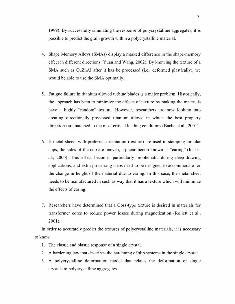
Importance of predicting crystal response
As mentioned earlier, “texture” is defined as the distribution of the orientations of
various crystals in a polycrystalline aggregate. A material having a “strong” texture has a
majority of the crystals having similar orientation. This gives rise to anisotropy within the
material. On the other hand, a material having a “weak” texture has the crystals oriented
in a much more “random” manner. We need to be able to predict the texture that a
material will attain after certain forming processes are performed on it. This will enable
us to create processes and materials that take advantage of the texture of the material.
Some examples where the ability to predict the crystal response would be an asset are
1. In the case of a simple pinned-pinned column, for a homogenous material with
fixed geometry, the critical buckling load is seen to be a linear function of the
Young’s modulus of the material. For copper polycrystals, this modulus can vary
from 66.7 GPa to 156.4 GPa (Mason and Maudlin, 1999). For designing a simple
pinned-pinned copper column, it can be seen that a “Wire” texture, with a
Young’s modulus of 156.4 GPa, would be preferred as it would be able to
withstand a higher load.
2. In nanocrystalline materials, it has been shown that non-equilibrium grain
boundaries in polycrystalline materials can form equilibrium grain boundaries by
the process of diffusive flow of atoms towards the grain boundaries (Bachurin et
al., 2003). The flow of atoms is governed by the difference in energy between two
neighboring crystals, which in turn depends upon the stress in the crystal.
3. In polycrystalline materials subjected to arbitrary strains, a phenomenon known as
grain growth takes place. During grain growth, grains with a lower energy grow at
the expense of grains having a higher energy. The process takes place in such a
way that the total energy of the polycrystalline material is lowered (Ono et al.,
3
1999). By successfully simulating the response of polycrystalline aggregates, it is
possible to predict the grain growth within a polycrystalline material.
4. Shape Memory Alloys (SMAs) display a marked difference in the shape-memory
effect in different directions (Yuan and Wang, 2002). By knowing the texture of a
SMA such as CuZnAl after it has be processed (i.e., deformed plastically), we
would be able to use the SMA optimally.
5. Fatigue failure in titanium alloyed turbine blades is a major problem. Historically,
the approach has been to minimize the effects of texture by making the materials
have a highly “random” texture. However, researchers are now looking into
creating directionally processed titanium alloys, in which the best property
directions are matched to the most critical loading conditions (Bache et al., 2001).
6. If metal sheets with preferred orientation (texture) are used in stamping circular
cups, the sides of the cup are uneven, a phenomenon known as “earing” (Inal et
al., 2000). This effect becomes particularly problematic during deep-drawing
applications, and extra processing steps need to be designed to accommodate for
the change in height of the material due to earing. In this case, the metal sheet
needs to be manufactured in such as way that it has a texture which will minimize
the effects of earing.
7. Researchers have determined that a Goss-type texture is desired in materials for
transformer cores to reduce power losses during magnetization (Rollett et al.,
2001).
In order to accurately predict the textures of polycrystalline materials, it is necessary
to know
1. The elastic and plastic response of a single crystal.
2. A hardening law that describes the hardening of slip systems in the single crystal.
3. A polycrystalline deformation model that relates the deformation of single
crystals to polycrystalline aggregates.
4
A brief history of crystal response theories
Various theories have been proposed for describing the response of crystalline
materials. These theories fall into two broad categories:
1. Theories that describe the response of single crystals subjected to arbitrary
deformations.
2. Theories that relate the response of single crystals to the response of
polycrystalline aggregates.
We shall consider these two categories in the following pages.
Deformation of single crystals
If an arbitrary deformation is applied to a crystal, it accommodates this
deformation by the process of shearing on crystallographic slip planes. This mechanism
is known as slip. Any crystal has a small number of slip systems available for slipping.
Consequently, the arbitrary deformation is accommodated by a combination of rigid
rotation and slipping.
One method in common use involves treating the incremental deformation in a
crystal as being the sum of two independent atomic mechanisms (Hill, 1966). On a
macroscopic level, these mechanisms have the following effect: (i) An overall elastic
distortion of the lattice and (ii) A plastic distortion of the crystal. It is important to note
that the lattice geometry remains unchanged in during the plastic part of the deformation.
Lee has presented a theory for describing the behavior of crystals to which an arbitrary
strain is applied (Lee, 1969). Lee’s paper describes the kinematics of crystal deformation
for elastic-plastic deformations at finite strains.
5
Mechanism of slip
The plastic deformation of metals takes place by two mechanisms: slip and
twinning. Plastic deformation occurs primarily by sliding of atoms along certain preferred
directions, known as slip directions. It has been proved that the simultaneous operation of
at least five independent slip systems is required to maintain continuity at grain
boundaries in a polycrystalline solid, if the deformations of individual grains are treated
as homogenous (Taylor, 1938). In the absence of five independent slip systems, the
deformation is accommodated by twinning (Hertzberg, 1976). The case where five
independent slip systems are unavailable to the crystal occurs when the crystal is forced
to undergo an extremely high deformation. In this thesis, we shall focus on deformation
of materials due to slip.
A slip system is defined by two factors:
1. The slip plane Normal – This is a normal to the plane that contains the slip
direction.
2. The slip direction – This is the direction along which the material slips, if the slip
system is activated.
The slip system parameters (slip plane Normal and direction) are determined by
the atomic packing of the individual atoms within the material. Therefore, we find that
the slip system parameters for Face Centered Cubic (FCC) materials are quite different
than those for Body Centered Cubic (BCC) and Hexagonal Close Packed (HCP)
materials. In our simulation, we shall mainly focus on FCC materials. However, the
software, that will be described presently, is written in such a manner that the user can
specify the number of slip systems as well as the slip system parameters.
Each slip system has a Critical Resolved Shear Stress (CRSS) associated with it.
Any stress imposed on the crystal can be projected onto each slip system. For a slip
system to be activated, the projected stress must exceed the CRSS on that slip system.
6
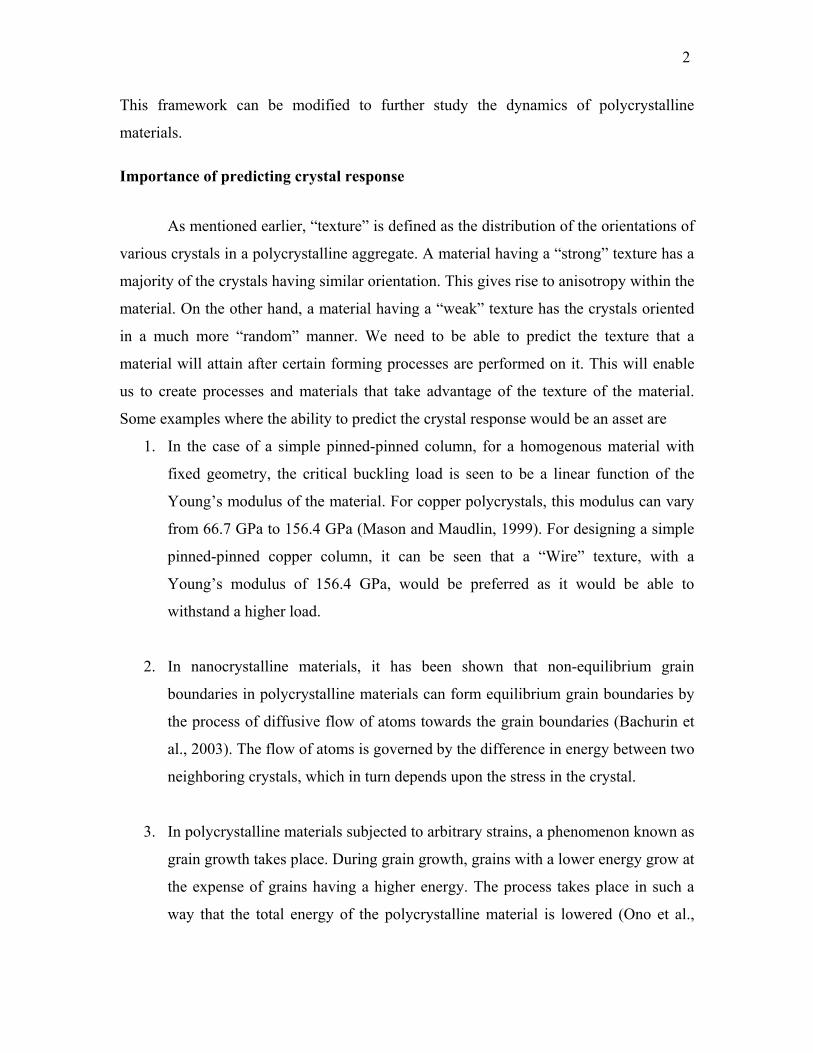
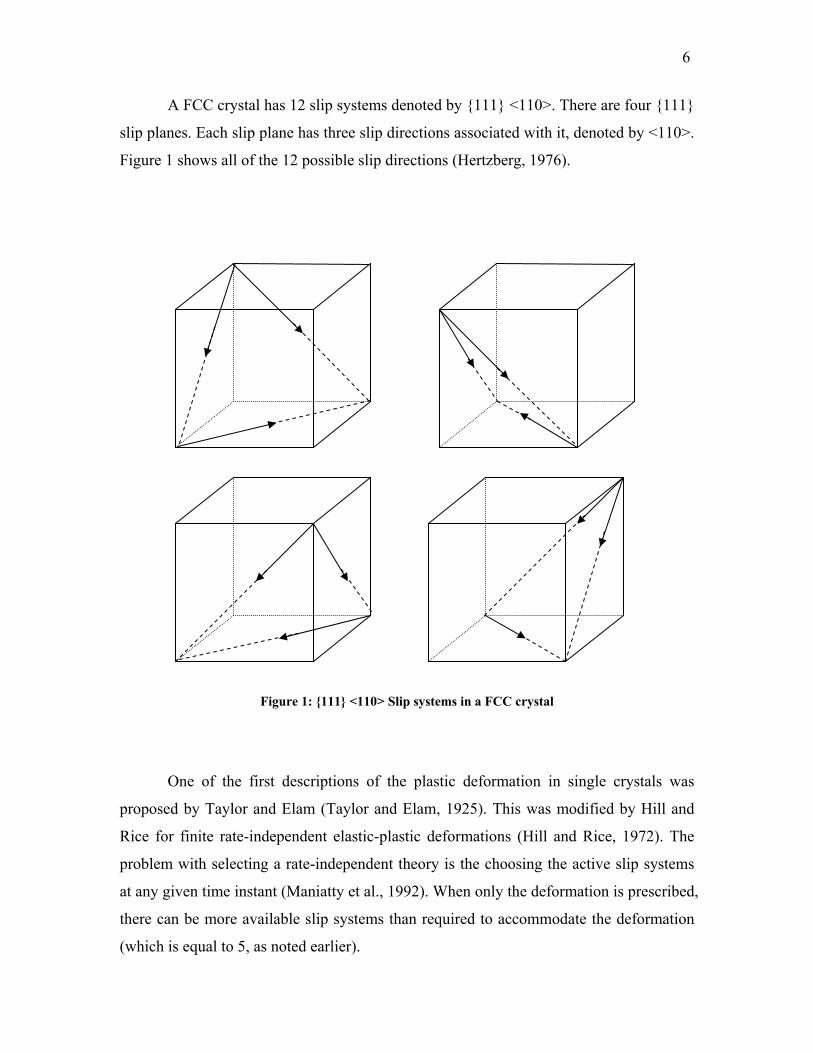
A FCC crystal has 12 slip systems denoted by {111} <110>. There are four {111}
slip planes. Each slip plane has three slip directions associated with it, denoted by <110>.
shows all of the 12 possible slip directions (Hertzberg, 1976). Figure 1
Figure 1: {111} <110> Slip systems in a FCC crystal
One of the first descriptions of the plastic deformation in single crystals was
proposed by Taylor and Elam (Taylor and Elam, 1925). This was modified by Hill and
Rice for finite rate-independent elastic-plastic deformations (Hill and Rice, 1972). The
problem with selecting a rate-independent theory is the choosing the active slip systems
at any given time instant (Maniatty et al., 1992). When only the deformation is prescribed,
there can be more available slip systems than required to accommodate the deformation
(which is equal to 5, as noted earlier).
7
Pan and Rice proved that for agreement with experimental results, it is necessary
to assume a rate-dependent model (Pan and Rice, 1983). For example, a superimposed
shear during compressive loading was found to produce an initially elastic response. This
could be explained only if the slipping was assumed to be rate-dependent. In this rate-
dependent model, the shearing rates are uniquely related to the stress state and the
material state.
Canova et al. have also discussed the effect of rate sensitivity on slip system
activity and lattice rotation (Canova et al., 1988). Most of the current models either (a)
neglect the elastic response completely, or (b) replace the elastic deformation gradient
with a rotation matrix which accounts for the rotation of the lattice, but does not consider
the elastic deformation.
Peirce et al. are among the few researchers who have included the elastic part of
the deformation gradient in their study on material rate dependence (Peirce et al., 1983).
Sarma and Zacharia have presented a novel integration scheme which directly calculates
the elastic deformation gradient of a crystal with respect to time (Sarma and Zacharia,
1999).
Hardening of slip systems
When a slip system activates, it causes the dislocations to move along the slip
direction. This causes a buildup of dislocations along that slip direction. This buildup
gives rise to a phenomenon known as “work hardening”. The higher the deformation of
the crystal, the more work is required to be done on it in order to cause further
deformation of the crystal.
As the dislocations pileup along a slip system, a larger stress has to be applied in
order to activate that slip system. In other words, the Critical Resolved Shear Stress
8
(CRSS) of that slip system increases. The CRSS is also referred to as the Hardness of the
slip system in this dissertation.
An accurate hardening law is of crucial importance in predicting the response of a
single crystal. As the future plastic deformation of the material is dependent upon the
current CRSS on all slip systems, it is necessary to pay great attention to selecting the
hardening law to be used.
Most of the models developed till date use a power law to describe the hardening
of slip systems which was first described by Hutchinson (Hutchinson, 1976). This law
assumes an equal hardening rate on all the slip systems. A quick glance at the mechanics
of slip, however, will show that a more advanced formulation is needed which takes into
account the different hardening rates on different slip systems.
Kocks and Mecking have pointed out that a modified Voce law appears to fit the
hardening data for a large range of stress-strain values (Kocks and Mecking, 2003). The
modified law requires the calculation of a scaling stress for each slip system at each time
step. Mecking et al. have proposed a “universal” FCC hardening law (Mecking et al.,
1986). This law manages to integrate the scaling-stress versus strain rate curves for FCC
materials over a wide range of temperature into one master curve.
Deformation of polycrystalline materials
There are a number of theories that attempt to relate the deformation of single
crystals to the deformation of polycrystals. One of the first attempts was by Taylor, which
assumed that the strain on any crystal within a polycrystalline material is the same as the
strain on the polycrystalline aggregate (Taylor, 1938). This model has been found to give
acceptable texture prediction for materials having high crystal symmetry and low rate
sensitivity (the Taylor model is a rate-independent model). While this model ensures
compatibility by prescribing an identical deformation on all crystals, the equilibrium
9
across grain boundaries is violated. The Sachs model (put forth in 1928), on the other
hand, postulates that the stress on each crystal within a polycrystalline aggregate is the
same. The Sachs model ensures equilibrium across grain boundaries, but in the process, it
violates compatibility across grain boundaries.
Additionally, these theories consider each crystal within the aggregate as an
independent entity which does not interact with neighboring grains. As pointed by Van
Houtte et al., the Taylor hypothesis predicts textures in which the locations of final
orientations can be “off” by 100, and the volume fractions can be off by a factor of 2 (Van
Houtte et al., 2002). To truly model the polycrystal response, it is necessary to consider
either a 2-point model (which considers the interaction of the crystal with its immediate
neighbor) or an n-point model (which considers the interaction of the crystal with “n”
other crystals). In this dissertation, an attempt is made for an n-point model by taking the
free energy of all crystals into account.
Research objectives
The overall goal of this dissertation is to provide a framework for simulating the
elastic and plastic response of single crystal and polycrystalline materials. With this in
mind, the following objectives are set to be achieved:
1. Implementing the algorithm outlined by Sarma and Zacharia (Sarma and Zacharia,
1999) to calculate the elastic deformation gradient of a single crystal subjected to
a prescribed velocity gradient. The plastic velocity gradient is also calculated and
stored, which can be used to view the development of the plastic deformation
gradient. The software should be written such that adapting it to BCC and HCP
materials should be a simple case of changing the input files passed to the
program. The user will be able to configure the following parameters:
a) Initial orientation of the crystal with respect to a fixed coordinate system.
b) Prescribed velocity gradient.
10
c) Slip systems
d) Material properties
e) Initial Hardness of slip systems
2. Changing the algorithm mentioned above to account for a more sophisticated
hardening law. The model proposed by Sarma and Zacharia assumes a simple law
that assumes uniform hardening for all the slip systems (Sarma and Zacharia,
1999). The hardening law outlined by Kocks and Mecking, and by Mecking et al.
allows us to calculate the hardening of each slip system uniquely, based on the
history of shearing rates on each slip system (Kocks and Mecking, 2003; Mecking
et al., 1986). The procedure for updating the Hardness of the slip systems with
time is to be written such that it can be easily changed to easily accommodate
future developments in the area of work hardening.
3. Proposing a theory for polycrystalline deformation. As pointed out before,
polycrystal models are more effective if the interaction between neighboring
grains is considered. The proposed theory shall use the concept of “free energy”
of the crystals and will take the energy of all crystals into account (creating, in
effect, an “n-point” model, with n = the number of crystals in the polycrystalline
aggregate).
Uniqueness of approach
This approach is unique in sense that it integrates two theories into one module:
1. Simulation of the elastic-plastic response of single crystals and the application of
this simulation to predicting the response of polycrystalline aggregates. The
simulation takes into account both the elastic and plastic parts of the total
deformation gradient of the crystal. The elastic part of the deformation gradient is
calculated directly.
11
2. The existence of a “universal” hardening law for FCC materials. This law fits the
experimental curves for FCC materials over a large range of temperatures. The
law also takes into account the fact that each slip system in a crystal has a
different hardening curve, which is based upon the history of shearing rates of that
particular slip system.
Another important facet of this work is the proposal of a theory for the
deformation of polycrystalline materials. This theory takes into account the free energies
of each crystal in a polycrystalline aggregate. This causes the response of each crystal to
be dependent upon its own state, as well as the states of all the other crystals in the
polycrystal. The theory will be set up in a way as to allow control over the amount of
compliance that each crystal exhibits with respect to the polycrystal, i.e., the deformation
of each crystal can be made to match the deformation of the polycrystal, or each crystal
can be allowed a certain amount of “freedom” in the deformation it undergoes in
response to the applied strain.
12
CHAPTER II
CRYSTAL MODEL
This chapter deals with the model used for describing the behavior of a single
crystal. An overview of polycrystalline models is also presented, the most prominent
among them being the Taylor and Sachs models. First, it is necessary to cover some of
the basic aspects of continuum mechanics.
Single crystal constitutive model
Reference configuration (C0)
Fp
Z
F* F
Y
Current configuration (C) X
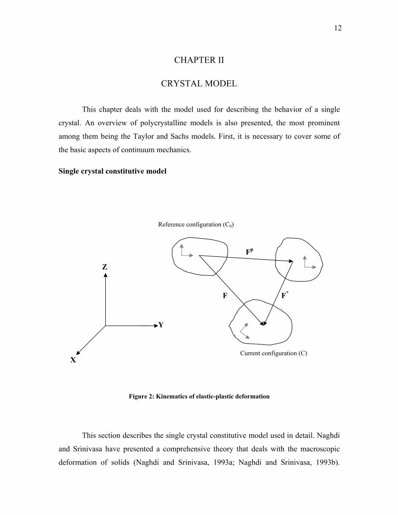
Figure 2: Kinematics of elastic-plastic deformation
This section describes the single crystal constitutive model used in detail. Naghdi
and Srinivasa have presented a comprehensive theory that deals with the macroscopic
deformation of solids (Naghdi and Srinivasa, 1993a; Naghdi and Srinivasa, 1993b).
13
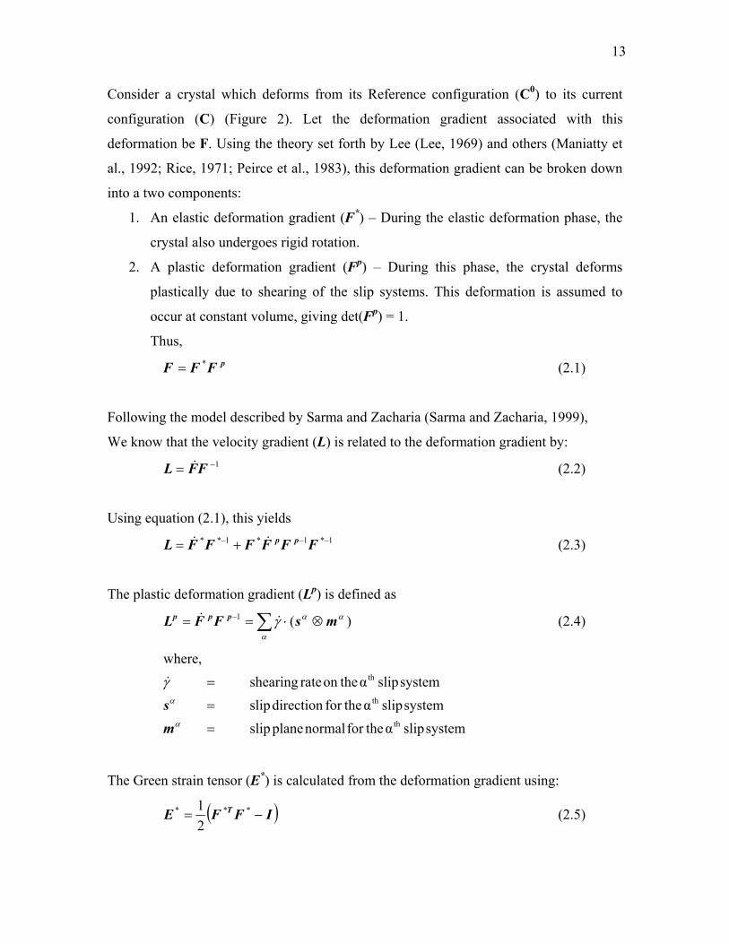
Consider a crystal which deforms from its Reference configuration (C0) to its current
configuration (C) ( ). Let the deformation gradient associated with this
deformation be F. Using the theory set forth by Lee (Lee, 1969) and others (Maniatty et
al., 1992; Rice, 1971; Peirce et al., 1983), this deformation gradient can be broken down
into a two components:
Figure 2
1. An elastic deformation gradient (F*) – During the elastic deformation phase, the
crystal also undergoes rigid rotation.
2. A plastic deformation gradient (Fp) – During this phase, the crystal deforms
plastically due to shearing of the slip systems. This deformation is assumed to
occur at constant volume, giving det(Fp) = 1.
Thus, pFFF *= (2.1)
Following the model described by Sarma and Zacharia (Sarma and Zacharia, 1999),
We know that the velocity gradient (L) is related to the deformation gradient by: 1−= FFL & (2.2)
Using equation (2.1), this yields 1*1*1** −−− += FFFFFFL pp&& (2.3)
The plastic deformation gradient (Lp) is defined as
∑ ⊗⋅== −
α
ααγ )(1 msFFL ppp && (2.4)
systemslipαthefornormalplaneslipsystemslipαthefordirectionslip
systemslipαtheonrateshearingwhere,
th
th
th
=
=
=
α
α
γ
ms
&
The Green strain tensor (E*) is calculated from the deformation gradient using:
( IFFE T −= ***
21 ) (2.5)
14
The second Piola-Kirchoff stress (T*) is given by:
][][ ** ELT = (2.6)
tensorelasticityorderfourth][where,
−=L
The shearing rate is given by:
)(ˆ
1
0α
α
αα τ
ττγγ sign
m&& = (2.7)
parameterysensitivitratesystemslipαtheforstressshearresolvedcriticalˆ
systemslipαthealongstressshearresolved
rateshearing)(referenceinitialwhere,
th
th0
==
=
=
m
α
α
τ
τ
γ&
The resolved shear stress on each slip system is given by:
)()()()( ** ααααααατ msTCmsTsTm ⊗⋅=⊗⋅=⋅= (2.8)
T
T
TFFFTTT
FFC
−−=
=
=
*1***
*
***
)(det:bytorelatediswhichtensor,stresscauchy
where,
The algorithm for implementing these equations is outlined in the paper by Sarma
and Zacharia (Sarma and Zacharia, 1999). It was also observed that keeping the Hardness
of the slip systems constant for the duration of a time step does not affect the calculations
15
by a noticeable degree. This simplifies the calculations, since the Hardness of the slip
systems has to be updated only at the end of each time step. The algorithm can be split
into two separate modules:
1. Calculating the elastic and plastic deformation gradients for a time step.
2. Updating the Hardness of the slip systems at the end of that time step.
Thus, to incorporate a new hardening law, we simply have to change the module
that updates the Hardness of the slip systems.
Algorithm
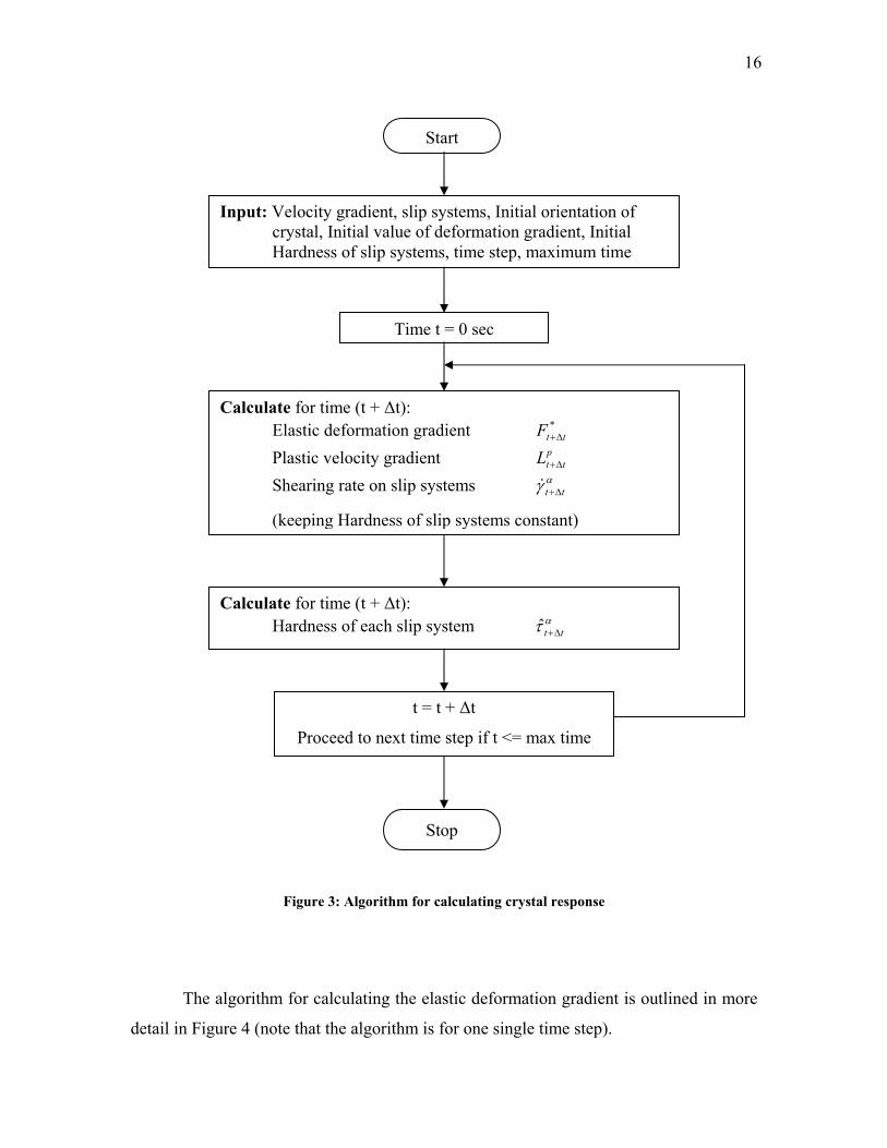
The algorithm for calculating the elastic deformation gradient for a crystal
subjected to an arbitrary deformation is described in detail by Sarma and Zacharia (Sarma
and Zacharia, 1999). This section provides an overview of that algorithm. The equations
to be used in calculating the elastic deformation gradient, the plastic velocity gradient and
the shearing rates have been given in the preceding pages. This algorithm is outlined in
. Figure 3
16
*ttF ∆+
pttL ∆+
αγ tt ∆+&
ατ tt ∆+ˆ
Start
Input: Velocity gradient, slip systems, Initial orientation of crystal, Initial value of deformation gradient, Initial Hardness of slip systems, time step, maximum time
Time t = 0 sec
Calculate for time (t + ∆t): Elastic deformation gradient Plastic velocity gradient
Shearing rate on slip systems
(keeping Hardness of slip systems constant)
Calculate for time (t + ∆t): Hardness of each slip system
t = t + ∆t
Proceed to next time step if t <= max time
Stop
Figure 3: Algorithm for calculating crystal response
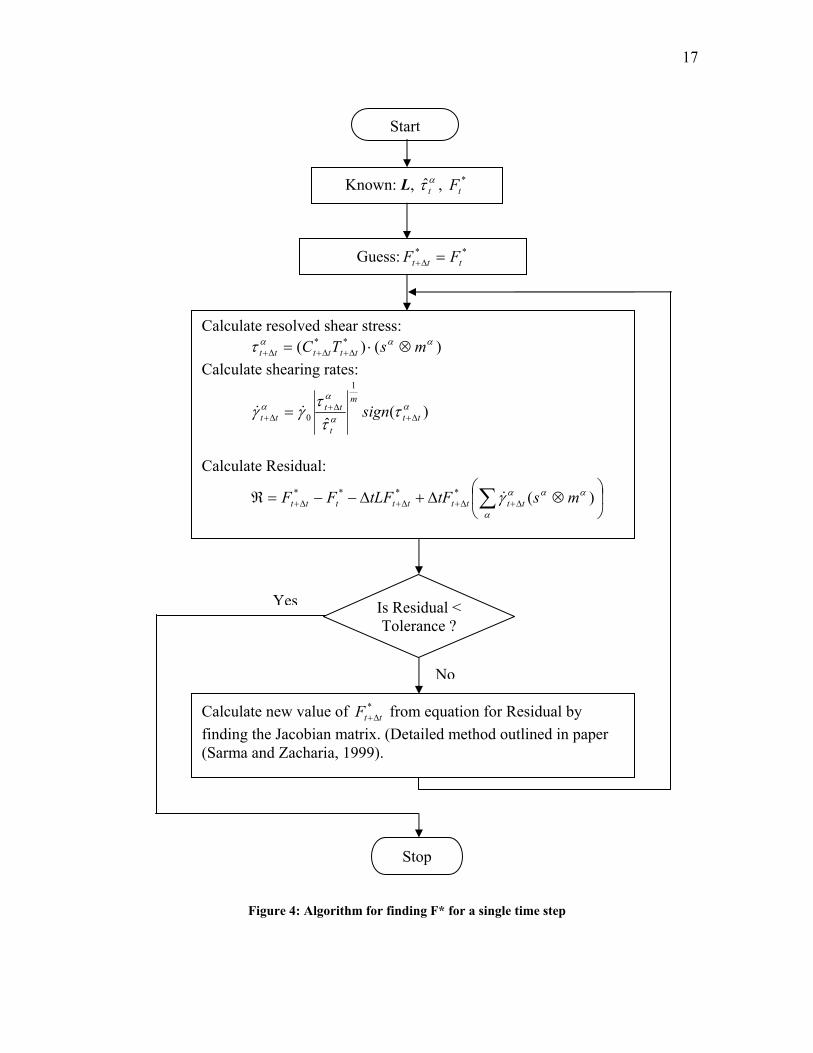
The algorithm for calculating the elastic deformation gradient is outlined in more
detail in (note that the algorithm is for one single time step). Figure 4
17
ατ tˆ*
t
**ttt FF =∆+
)()( ** ααατ msTC tttttt ⊗⋅= ∆+∆+∆+
)(ˆ
1
0α
α
αα τ
ττ
γγ tt
m
t
tttt sign ∆+
∆+∆+ = &&
⊗∆+∆−−=ℜ ∑ ∆+∆+∆+∆+
α
αααγ )(**** mstFtLFFF ttttttttt &
*ttF ∆+
Start
Known: L, , F
Guess:
Calculate resolved shear stress: Calculate shearing rates:
Calculate Residual:
Yes Is Residual < Tolerance ?
No
Calculate new value of from equation for Residual by finding the Jacobian matrix. (Detailed method outlined in paper (Sarma and Zacharia, 1999).
Stop
Figure 4: Algorithm for finding F* for a single time step
18
Hardening law for slip systems
In this section, a new hardening law for FCC materials is discussed. This
hardening law accounts for different hardening rates on for each slip system in the
material. The law has been found to fit the experimental data for a large number of FCC
materials, over a wide range of temperatures.
The Critical Resolved Shear Stress (CRSS, also known as Hardness) of each slip
system changes with time. Voce proposed a hardening law which takes the form:
−Θ=Θ
vσσ10 (2.9)
stressscalingcrystalonstress
constantratehardeningnet
where,
0
===Θ=Θ
vσσ
As pointed out by Kocks and Mecking (Kocks and Mecking, 2003), the Voce law
does not fit the stress-strain curves over the entire regime, but does give a reasonable fit
over a significant range of Θ/Θ0.
A modified hardening law suggested by Kocks and Mecking takes the form
(Kocks and Mecking, 2003): κ
κσσ
−Θ=Θ
v
10 (2.10)
constant empiricalstressscaling
crystalonstressconstant
ratehardeningnetwhere,
0
====Θ=Θ
κσσ
v
19
It is necessary at this point to digress a little, and explain the nature of hardening
laws. An important fact is that all hardening laws are theories, developed in order to
attempt to explain the observed response of loaded polycrystalline materials. A theory
that takes into account all the microscopic mechanisms (such as dislocations) would
involve an extremely high number of parameters (and statistical methods since it would
be impractical to measure each dislocation in a material). As a result, researchers attempt
to develop theories such that the predicted stress-strain response of a material will closely
match the experimental results.
Since the stresses and strains on individual crystals in a polycrystalline material
cannot be directly measured, they must be approximated. The most common theory used
is the Taylor model, which assumes that the strain on each crystal is the same as the strain
on the polycrystalline material (Taylor, 1938).
In equations (2.9) and (2.10), the quantity Θ = dσ / dγ. Here σ represents the stress
on the polycrystal, and γ denotes the strain. These quantities can be measured
experimentally. The corresponding single-crystal quantities, i.e., τ and ε cannot be
measured experimentally. The assumption made at this point is that Θ in the above
equations can be replaced with its single-crystal counterpart, namely θ = dτ / dε. Finally,
note that the expression dτ / dε does not imply that τ is a function of ε (even though it
appears to be so due to the way it is written). The actual expression should be:dtddtd
//
ετθ = .
Using our notation for variables in equation (2.10), the hardening law will take
the form
20
ακα
α γκσττ && ⋅
−Θ=
v
1ˆ 0 (2.11)
systemslipαonrateshearing
stressscaling2003) Mecking, and (Kocks 1.3constantempirical
systemslipαtheonstressshearresolved
constantsystemslipαtheofhardnessofderivativeTimeˆ
where,
th
th0
th
=
===
=
=Θ=
α
α
α
γ
σκτ
τ
&
&
v
To apply the hardening law on our algorithm, let us consider each variable in turn:
• - This is the time derivative of the Hardness of the αατ&̂ th slip system. Once we
find this quantity, we can update the Hardness of each slip system.
• - This is a constant, and can be calculated from experimental results. The
procedure for selecting is outlined by Mecking et al. (Mecking et al., 1986)
0Θ
0Θ
• - This is the resolved shear stress on the αατ th slip system. This can be calculated
from equation (2.8).
• κ – empirical constant = 1.3 (Kocks and Mecking, 2003).
• σv – scaling stress, to be determined.
• - shearing rate on the ααγ& th slip system. This can be calculated from equation (2.7)
Thus, we can see that, for using the hardening law given in Equation (2.11), the only
thing we need to determine is a suitable scaling stress (σv) for each slip system at the end
of each time step.
21
Determining the scaling stress
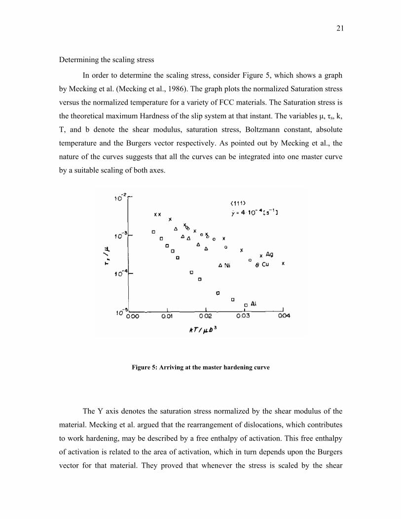
In order to determine the scaling stress, consider Figure 5, which shows a graph
by Mecking et al. (Mecking et al., 1986). The graph plots the normalized Saturation stress
versus the normalized temperature for a variety of FCC materials. The Saturation stress is
the theoretical maximum Hardness of the slip system at that instant. The variables µ, τs, k,
T, and b denote the shear modulus, saturation stress, Boltzmann constant, absolute
temperature and the Burgers vector respectively. As pointed out by Mecking et al., the
nature of the curves suggests that all the curves can be integrated into one master curve
by a suitable scaling of both axes.
Figure 5: Arriving at the master hardening curve
The Y axis denotes the saturation stress normalized by the shear modulus of the
material. Mecking et al. argued that the rearrangement of dislocations, which contributes
to work hardening, may be described by a free enthalpy of activation. This free enthalpy
of activation is related to the area of activation, which in turn depends upon the Burgers
vector for that material. They proved that whenever the stress is scaled by the shear
22
modulus of the material, the temperature must be scaled by the quantity µb3. The X axis
in the above figure denotes the normalized temperature multiplied by the Boltzmann
constant of the material.
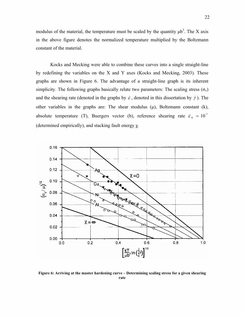
Kocks and Mecking were able to combine these curves into a single straight-line
by redefining the variables on the X and Y axes (Kocks and Mecking, 2003). These
graphs are shown in . The advantage of a straight-line graph is its inherent
simplicity. The following graphs basically relate two parameters: The scaling stress (σv)
and the shearing rate (denoted in the graphs by ε& , denoted in this dissertation by γ&
0 =
). The
other variables in the graphs are: The shear modulus (µ), Boltzmann constant (k),
absolute temperature (T), Buergers vector (b), reference shearing rate
(determined empirically), and stacking fault energy χ.
710ε&
Figure 6
Figure 6: Arriving at the master hardening curve – Determining scaling stress for a given shearing rate
23
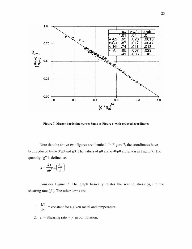
Figure 7: Master hardening curve: Same as Figure , with reduced coordinates 6
Note that the above two figures are identical. In Figure 7, the coordinates have
been reduced by σv0/µ0 and g0. The values of g0 and σv0/µ0 are given in Figure 7. The
quantity “g” is defined as
=εε
µ &
&03 ln
bkTg
Consider Figure 7. The graph basically relates the scaling stress (σv) to the
shearing rate (γ& ). The other terms are:
1. 3µbkT = constant for a given metal and temperature.
2. ε& = Shearing rate = γ& in our notation.

24
3. (Kocks and Mecking, 2003). 170 10 −= sε&
Thus, using the graphs from Figure 7, we can obtain a suitable scaling stress (σv) for each
time step. Once the scaling stress is obtained, it is a simple matter of plugging it into
equation (2.11) to obtain the hardening rate.
To summarize, the following steps have to be followed at the end of each time
step in order to update the Hardness of the slip systems according to the hardening law
outlined above:
1. Determine the scaling stress (σv) at the end of each time step from the graphs
shown in
2. Figure 7. Each slip system will have a unique scaling stress based on its shearing
rate.
3. Find the hardening rate for each slip system for that time step ( ) using
Equation (2.11).
ατ&̂
4. Update the Hardness of each slip system for that time step by using. ααα τττ tttt t &̂ˆˆ ⋅∆+=∆+
25
Deformation of polycrystalline aggregates
In this section, an attempt is made to arrive at a theory for relating the response of
single crystals to polycrystalline materials. As stated before, there are currently two major
theories in use: The Taylor hypothesis, which assumes the strain to be the same for all
crystals, and the Sachs model, which assumes the stress of each crystal to be the same.
The Taylor hypothesis works best when the crystals in a polycrystalline aggregate have
orientations which are similar to each other. While this model ensures compatibility by
prescribing an identical deformation on all crystals, the equilibrium across grain
boundaries is violated. The Sachs model ensures equilibrium across grain boundaries, but
in the process, it violates compatibility across grain boundaries. Other theories assume
the polycrystal to be made up of a number of ellipsoids embedded in a homogenous
matrix. By choosing the relationships between the matrix and the medium, different
averaging schemes are obtained. Some examples of these are self-consistent models and
the Mori-Tanaka model (Mori and Tanaka, 1973).
An attempt is made to arrive at a formulation wherein the relationship between
the single crystal and polycrystal response can be adjusted to vary from a Taylor type
model to a Sachs type model. This attempt treats each crystal as an individual entity
without considering the interaction between neighboring crystals. This theory is
presented as an example of how the single crystal solver can be used to try out various
theories relating the single crystal response to polycrystal response.
The following conventions are used to distinguish single crystal variables from
polycrystal variables:
1. Single crystal variables have a superscript of “(i)”, which indicates that the
variable represents the ith crystal. The superscript is appended before any existing
superscripts (e.g. “*” for indicating the elastic part of the deformation).
Examples: F(i), F(i)*, F(i)p, L(i)
26
2. Polycrystal variables have the usual superscripts for denoting elastic and plastic
parts.
Examples: F, F*, Fp, L
Let α(i) denote the volume fraction of the ith crystal in the polycrystalline aggregate.
( 1)We have: )( =∑i
iα
∑=i
ii FF )()(α (2.12)
crystalitheofgradientndeformatiooverallaggregatellinepolycrysta ofgradient ndeformatiooverall
where,
th)( =
=iF
F
The above equation can also be written in the form
[ ] 0)()( =−∑i
ii FFα (2.13)
We assume that the stored energy in the ith crystal is given by the sum of
1. Ψ1 – The stored energy of deformation in the ith crystal, and
2. Ψ2 – The energy due to the difference in the deformation between neighboring
crystals.
[ ] [ ])()(2
)*()(1
)( iiiii FFF −Ψ+Ψ=Ψ (2.14)
We assume that Ψ2 takes the form [ ] [ ])()(
2ii FFFF −⋅−
µ . If a crystal has a
deformation that is significantly different from the mean deformation of the
polycrystalline aggregate, its interaction energy (Ψ2) will be higher.
Thus, equation (2.14) becomes
[ ] [ ] [ ])()()*()(1
)(
2iiiii FFFFF −⋅−+Ψ=Ψ
µ (2.15)
27
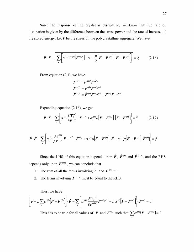
Since the response of the crystal is dissipative, we know that the rate of
dissipation is given by the difference between the stress power and the rate of increase of
the stored energy. Let P be the stress on the polycrystalline aggregate. We have
[ ] [ ] [ ] ξµαα =
−⋅−+Ψ−⋅
⋅
∑i
iiiiii FFFFFFP )()()(*)()(1
)(
2& (2.16)
From equation (2.1), we have
1)()(1)()(*)(
1)()(*)(
)(*)()(
−−
−
+=
=
=
piipiii
piii
piii
FFFFFFFFFFF
&&&
Expanding equation (2.16), we get
[ ] [ ] ξµαα =
−⋅−+⋅
∂Ψ∂
−⋅ ∑i
iiiii
ii FFFFF
FFP )()()()*(
)*(
)(1)( &&&& (2.17)
[ ] [ ] ξµαµαα =
⋅−−⋅−+⋅
∂Ψ∂
−⋅ ∑−
i
iiiiiipii
ii FFFFFFFF
FFP
T )()()()()()()()*(
)(1)( &&&&
Since the LHS of this equation depends upon F& , )(iF& and piF )(& , and the RHS
depends only upon piF )(& , we can conclude that
1. The sum of all the terms involving F& and )(iF& = 0.
2. The terms involving piF )(& must be equal to the RHS.
Thus, we have
[ ] [ ] 0)()()()()*(
)(1)()()( =⋅
−−
∂Ψ∂
−⋅
−− ∑∑
− i
i
iipii
ii
i
ii FFFFF
FFFPT && µαααµ
This has to be true for all values of F& and )(iF& such that ( ) 0)()( =−∑i
ii FF &&α .
28
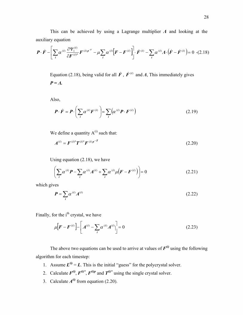
This can be achieved by using a Lagrange multiplier Λ and looking at the
auxiliary equation
[ ] ( ) 0)()()()()()()*(
)(1)( =−⋅−⋅
−−
∂Ψ∂
−⋅ ∑∑∑−
i
iii
i
ii
i
pii
ii FFΛFFFF
FFP
T &&&& ααµα -(2.18)
Equation (2.18), being valid for all F& , )(iF& and Λ, This immediately gives
P = Λ.
Also,
(∑∑ ⋅=
⋅=⋅
i
ii
i
ii FPFPFP )()()()( αα& ) (2.19)
We define a quantity A(i) such that: Tpiiii FTFA −
= )(*)(*)()( (2.20)
Using equation (2.18), we have
( ) 0)()()()()( =
−+− ∑∑∑ i
i
ii
i
i
i
i FFAP µααα (2.21)
which gives )()( i
i
i AP ∑= α (2.22)
Finally, for the ith crystal, we have
[ ] 0)()()()( =
−−− ∑
i
iiii AAFF αµ (2.23)
The above two equations can be used to arrive at values of F(i) using the following
algorithm for each timestep:
1. Assume L(i) = L. This is the initial “guess” for the polycrystal solver.
2. Calculate F(i), F(i)*, F(i)p and T(i)* using the single crystal solver.
3. Calculate A(i) from equation (2.20).
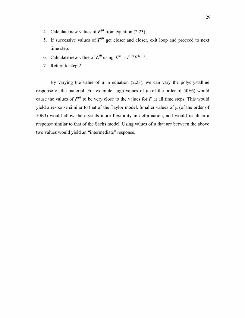
29
4. Calculate new values of F(i) from equation (2.23).
5. If successive values of F(i) get closer and closer, exit loop and proceed to next
time step.
6. Calculate new value of L(i) using 1)()()( −= iii FFL & .
7. Return to step 2.
By varying the value of µ in equation (2.23), we can vary the polycrystalline
response of the material. For example, high values of µ (of the order of 50E6) would
cause the values of F(i) to be very close to the values for F at all time steps. This would
yield a response similar to that of the Taylor model. Smaller values of µ (of the order of
50E3) would allow the crystals more flexibility in deformation, and would result in a
response similar to that of the Sachs model. Using values of µ that are between the above
two values would yield an “intermediate” response.
30
CHAPTER III
USING THE PROGRAM “CRYSTALS”
“Crystals” is an interactive program that enables the user to simulate the loading
of a single crystal or a polycrystalline material. Each simulation is described by a
“project”. There are two basic types of projects – Single crystal projects, and Polycrystal
projects. Each project consists of a set of files, namely:
1. A Project file (having an extension of “.proj”)
2. Input files (having an extension of “.in”)
3. Output files (having an extension of “.out”). Output files are generated by the
software.
File formats for project and input files
The program has a Graphical User Interface, which can be used to enter various
parameters. In order to use the interface, it is first essential to have an understanding of
the formats of project and input files. The following sections describe these file formats.
All project and input files are to be supplied in plain ASCII format. The specific
format of each type of file is described in the following pages. Text that is enclosed
within “< >” stands for a variable. For example, <type of project> on a line means that
the user should enter the “type of project” on that line, which can be: 0 for a Single
crystal project, or 1 for a Polycrystal project. All other text is to be entered in the file as it
is.
31
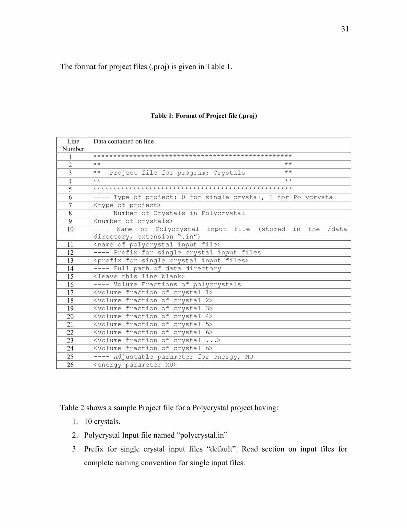
The format for project files (.proj) is given in Table 1.
Table 1: Format of Project file (.proj)
Line
Number Data contained on line
1 ************************************************** 2 ** ** 3 ** Project file for program: Crystals ** 4 ** ** 5 ************************************************** 6 ---- Type of project: 0 for single crystal, 1 for Polycrystal 7 <type of project> 8 ---- Number of Crystals in Polycrystal 9 <number of crystals> 10 ---- Name of Polycrystal input file (stored in the /data
directory, extension “.in”) 11 <name of polycrystal input file> 12 ---- Prefix for single crystal input files 13 <prefix for single crystal input files> 14 ---- Full path of data directory 15 <leave this line blank> 16 ---- Volume Fractions of polycrystals 17 <volume fraction of crystal 1> 18 <volume fraction of crystal 2> 19 <volume fraction of crystal 3> 20 <volume fraction of crystal 4> 21 <volume fraction of crystal 5> 22 <volume fraction of crystal 6> 23 <volume fraction of crystal ...> 24 <volume fraction of crystal n> 25 ---- Adjustable parameter for energy, MU 26 <energy parameter MU>
Table 2 shows a sample Project file for a Polycrystal project having:
1. 10 crystals.
2. Polycrystal Input file named “polycrystal.in”
3. Prefix for single crystal input files “default”. Read section on input files for
complete naming convention for single input files.
32
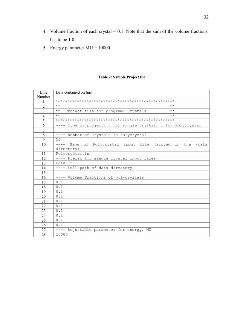
4. Volume fraction of each crystal = 0.1. Note that the sum of the volume fractions
has to be 1.0.
5. Energy parameter MU = 10000
Table 2: Sample Project file
Line
Number Data contained on line
1 ************************************************** 2 ** ** 3 ** Project file for program: Crystals ** 4 ** ** 5 ************************************************** 6 ---- Type of project: 0 for single crystal, 1 for Polycrystal 7 1 8 ---- Number of Crystals in Polycrystal 9 10 10 ---- Name of Polycrystal input file (stored in the /data
directory) 11 Polycrystal.in 12 ---- Prefix for single crystal input files 13 Default 14 ---- Full path of data directory 15 16 ---- Volume Fractions of polycrystals 17 0.1 18 0.1 19 0.1 20 0.1 21 0.1 22 0.1 23 0.1 24 0.1 25 0.1 26 0.1 27 ---- Adjustable parameter for energy, MU 28 10000
33
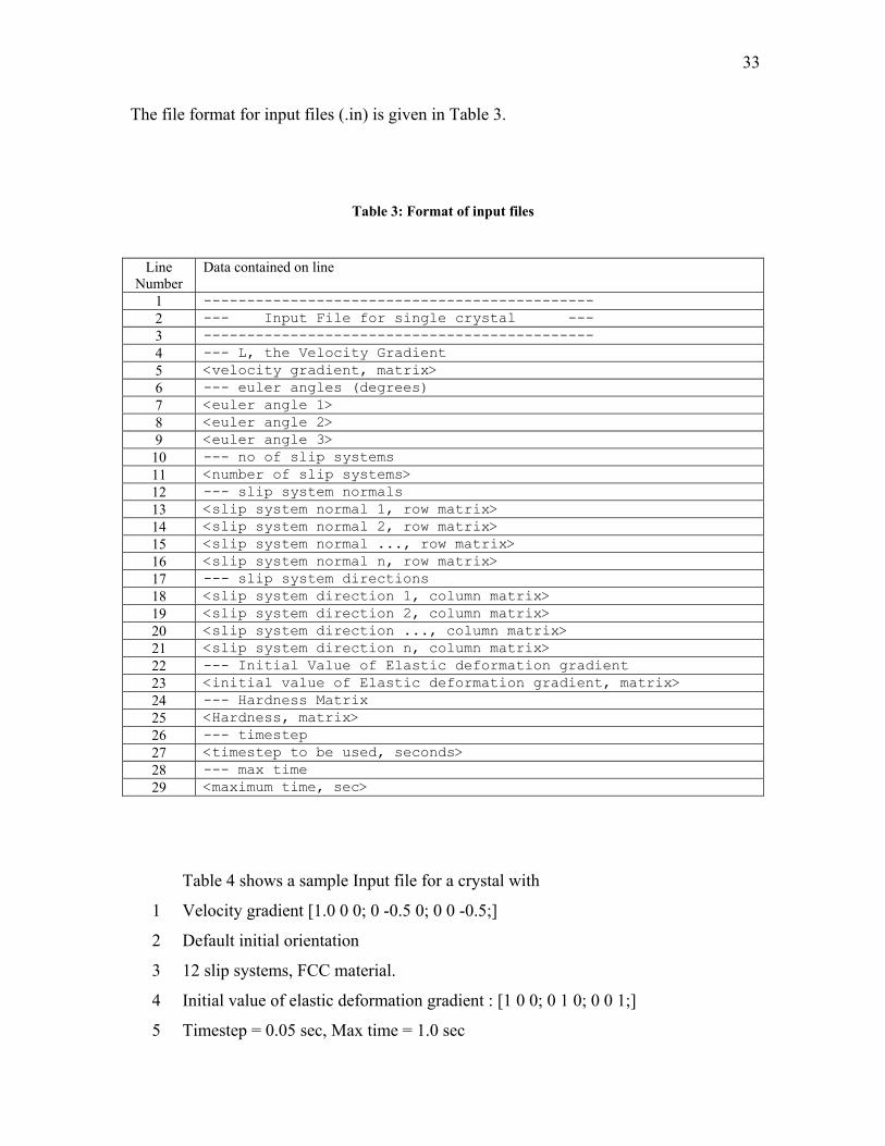
The file format for input files (.in) is given in . Table 3
Table 3: Format of input files
Line
Number Data contained on line
1 --------------------------------------------- 2 --- Input File for single crystal --- 3 --------------------------------------------- 4 --- L, the Velocity Gradient 5 <velocity gradient, matrix> 6 --- euler angles (degrees) 7 <euler angle 1> 8 <euler angle 2> 9 <euler angle 3> 10 --- no of slip systems 11 <number of slip systems> 12 --- slip system normals 13 <slip system normal 1, row matrix> 14 <slip system normal 2, row matrix> 15 <slip system normal ..., row matrix> 16 <slip system normal n, row matrix> 17 --- slip system directions 18 <slip system direction 1, column matrix> 19 <slip system direction 2, column matrix> 20 <slip system direction ..., column matrix> 21 <slip system direction n, column matrix> 22 --- Initial Value of Elastic deformation gradient 23 <initial value of Elastic deformation gradient, matrix> 24 --- Hardness Matrix 25 <Hardness, matrix> 26 --- timestep 27 <timestep to be used, seconds> 28 --- max time 29 <maximum time, sec>
Table 4 shows a sample Input file for a crystal with
1 Velocity gradient [1.0 0 0; 0 -0.5 0; 0 0 -0.5;]
2 Default initial orientation
3 12 slip systems, FCC material.
4 Initial value of elastic deformation gradient : [1 0 0; 0 1 0; 0 0 1;]
5 Timestep = 0.05 sec, Max time = 1.0 sec
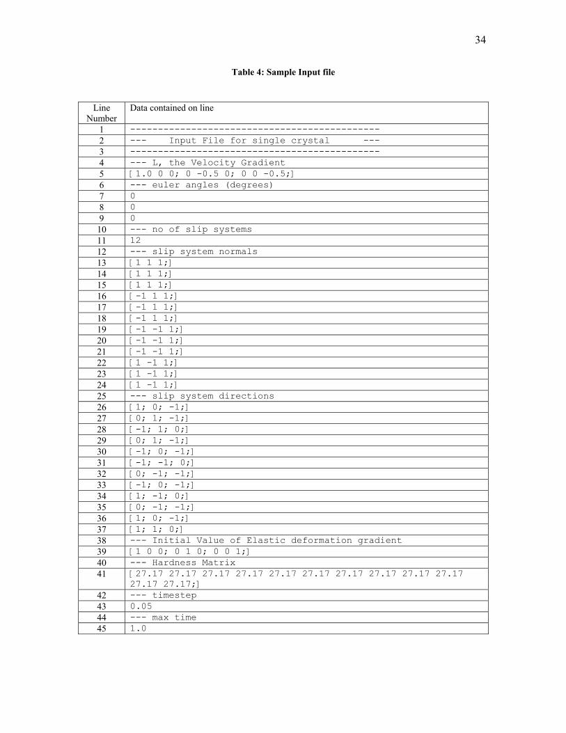
34
Table 4: Sample Input file
Line
Number Data contained on line
1 --------------------------------------------- 2 --- Input File for single crystal --- 3 --------------------------------------------- 4 --- L, the Velocity Gradient 5 [1.0 0 0; 0 -0.5 0; 0 0 -0.5;] 6 --- euler angles (degrees) 7 0 8 0 9 0 10 --- no of slip systems 11 12 12 --- slip system normals 13 [1 1 1;] 14 [1 1 1;] 15 [1 1 1;] 16 [-1 1 1;] 17 [-1 1 1;] 18 [-1 1 1;] 19 [-1 -1 1;] 20 [-1 -1 1;] 21 [-1 -1 1;] 22 [1 -1 1;] 23 [1 -1 1;] 24 [1 -1 1;] 25 --- slip system directions 26 [1; 0; -1;] 27 [0; 1; -1;] 28 [-1; 1; 0;] 29 [0; 1; -1;] 30 [-1; 0; -1;] 31 [-1; -1; 0;] 32 [0; -1; -1;] 33 [-1; 0; -1;] 34 [1; -1; 0;] 35 [0; -1; -1;] 36 [1; 0; -1;] 37 [1; 1; 0;] 38 --- Initial Value of Elastic deformation gradient 39 [1 0 0; 0 1 0; 0 0 1;] 40 --- Hardness Matrix 41 [27.17 27.17 27.17 27.17 27.17 27.17 27.17 27.17 27.17 27.17
27.17 27.17;] 42 --- timestep 43 0.05 44 --- max time 45 1.0
35
The output files generated by the program are in plain ASCII format, and can be
imported into other programs for analysis if needed.
The concepts of “Initial Orientation” and “Specifying Matrices” will be discussed
later on in this chapter.
Naming conventions for files in Polycrystal projects
The standard naming conventions for files are:
1 Project files - .proj
2 Input files - .in
3 Output files - .out
In case of Polycrystal projects, we must have
1. A Project file
2. A polycrystal Input file.
3. Initial input files for each of the single crystals that make up the polycrystal.
The initial input files for each of the single crystals should follow the follwing
convention: <single-crystal-file-prefix>-<crystal number>--1.in
For example, a project having <single-crystal-file-prefix> as “default” and having
10 crystals will have the following single-crystal input files:
default-0--1.in
default-1--1.in
default-2--1.in
default-3--1.in
default-4--1.in
default-5--1.in
default-6--1.in
default-7--1.in
default-8--1.in
default-9--1.in
36
The files generated by the program have the following convention:
Input files: <single-crystal-file-prefix>-<crystal number>-<timestep>.in
Output files: <single-crystal-file-prefix>-<crystal number>-<timestep>.out
For example, the program will generate the following files for crystal number 5,
timestep 3. (Note that both crystal number and timestep are zero-based)
default-5-3.in
default-5-3.out
Specifying matrices in input files
The program makes extensive use of matrices during the course of calculations.
Many parameters have to be specified as matrices. For example, the initial value of the
elastic deformation gradient is a 3x3 matrix. Slip System normals are specified as vectors
(row matrices) and Slip System directions are specified as vectors (column matrices).
Matrices can be specified by using initialization strings which are similar to the
initialization strings used by MATLAB. The program does not perform any error-
checking on the initialization string, and hence it is necessary to follow these rules strictly:
1. The first character of the initialization string must be "[". (without the quotes).
2. Elements on a row are separated by a space. There must be exactly ONE space
between two elements.
3. The end of a row is indicated by the ";" character. The ";" character must be
followed by exactly one space. The trailing space may be omitted if it is the last
row of the matrix.
4. The last character of the initialization string must be "]".
37
Here are some sample matrices and their initialization strings:
1. Identity matrix – [1 0 0; 0 1 0; 0 0 1;]
2. A 2 x 4 matrix – [1 6 2 6; 4 3 3 0;]
3. A row matrix – [1 -1 1;]
4. A column matrix – [1; -1; 1;]
5. Matrix with elements specified using scientific notation –
[1e34 -5e-30 5.4544;]
Specifying the initial orientation of a crystal
Every crystal can have a different orientation with respect to a fixed reference
frame. This orientation can be specified in the Input file with the help of three Euler
Angles.
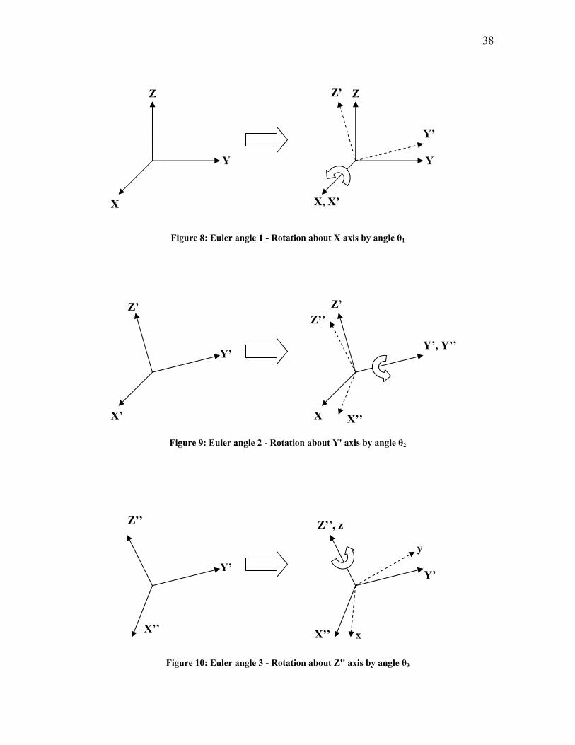
Consider the material to have a fixed reference frame, denoted by the axes X, Y
and Z. Let the coordinate axes of the crystal be denoted by x, y and z. A crystal can be
transformed from the reference coordinate system (X, Y, Z) to any arbitrarily oriented
system (x,y,z) using three rotations. These rotations are known as Euler angles, and these
can be entered into the input files to describe how the crystal is oriented with respect to
the material.
- demonstrate how three rotations can transform axes (X,Y,Z)
into axes (x,y,z).
Figure 8 Figure 10
38
Z’Z Z
Y’
Y Y
X, X’ X
Figure 8: Euler angle 1 - Rotation about X axis by angle θ1
Z’Z’ Z’’
Y’, Y’’ Y’
XX’ X’’
Figure 9: Euler angle 2 - Rotation about Y' axis by angle θ2
Z’’ Z’’, z
y
Y’ Y’
X’’ X’’ x
Figure 10: Euler angle 3 - Rotation about Z'' axis by angle θ3
39
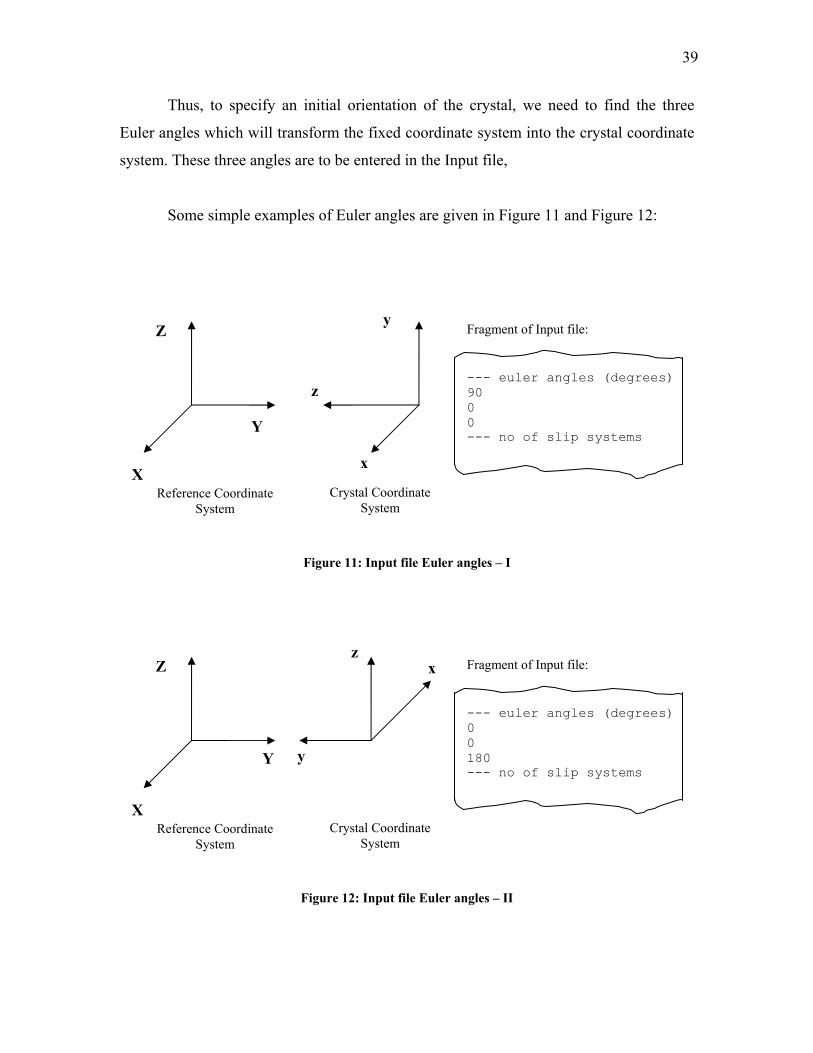
Thus, to specify an initial orientation of the crystal, we need to find the three
Euler angles which will transform the fixed coordinate system into the crystal coordinate
system. These three angles are to be entered in the Input file,
Some simple examples of Euler angles are given in Figure 11 and Figure 12:
y Z Fragment of Input file:
--- euler angles (degrees)
Figure 11: Input file Euler angles – I
Figure 12: Input file Euler angles – II
Y
Z
X
y
z
Reference Coordinate System
Crystal Coordinate System
Fragment of Input file: --- euler angles (degrees)0 0 180 --- no of slip systems
x
Y
X
z 90 0 0 --- no of slip systems
x
Crystal Coordinate Reference Coordinate System System
40
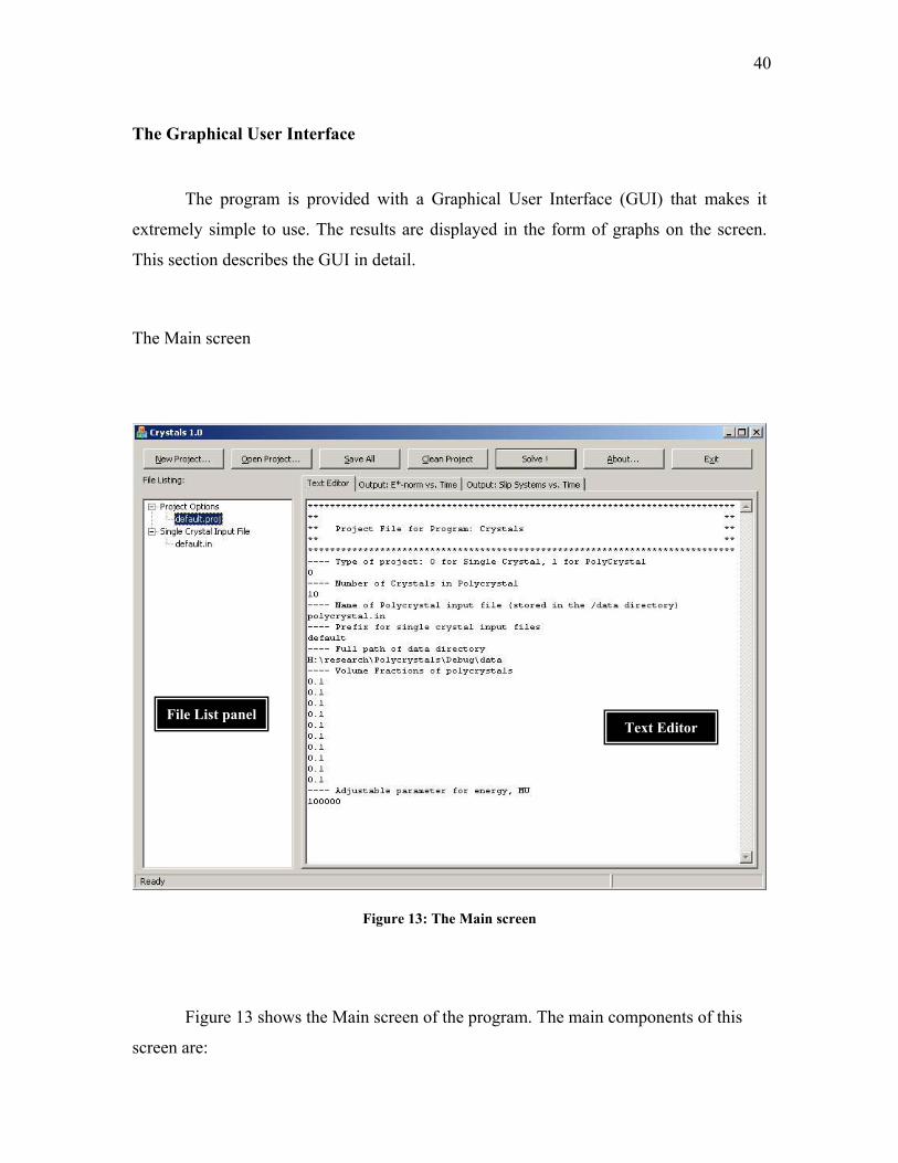
The Graphical User Interface
The program is provided with a Graphical User Interface (GUI) that makes it
extremely simple to use. The results are displayed in the form of graphs on the screen.
This section describes the GUI in detail.
The Main screen
File List panel Text Editor
Figure 13: The Main screen
Figure 13 shows the Main screen of the program. The main components of this
screen are:

41
1. t
is currently open.
it it.
Figure 14 shows the buttons that are available at the top of the Main screen:
The File List panel: This panel contains a listing of all input files for the projec
that
2. The Text Editor: This is a text editor built into the program. Select a file from
the File List panel to ed
Creates a new project.
Opens an existing project. The Project filename must have an extension of “.proj”
Saves all open file(s) in the text editor.
Deletes all intermediate input and output files (only for Polycrystal projects)
Fires up the Solver. Select one of the “Output:” tabs to splot of the results as th
ee a ey are calculated.
Displays information about the application
Exits the application
Figure 14: Buttons in the program
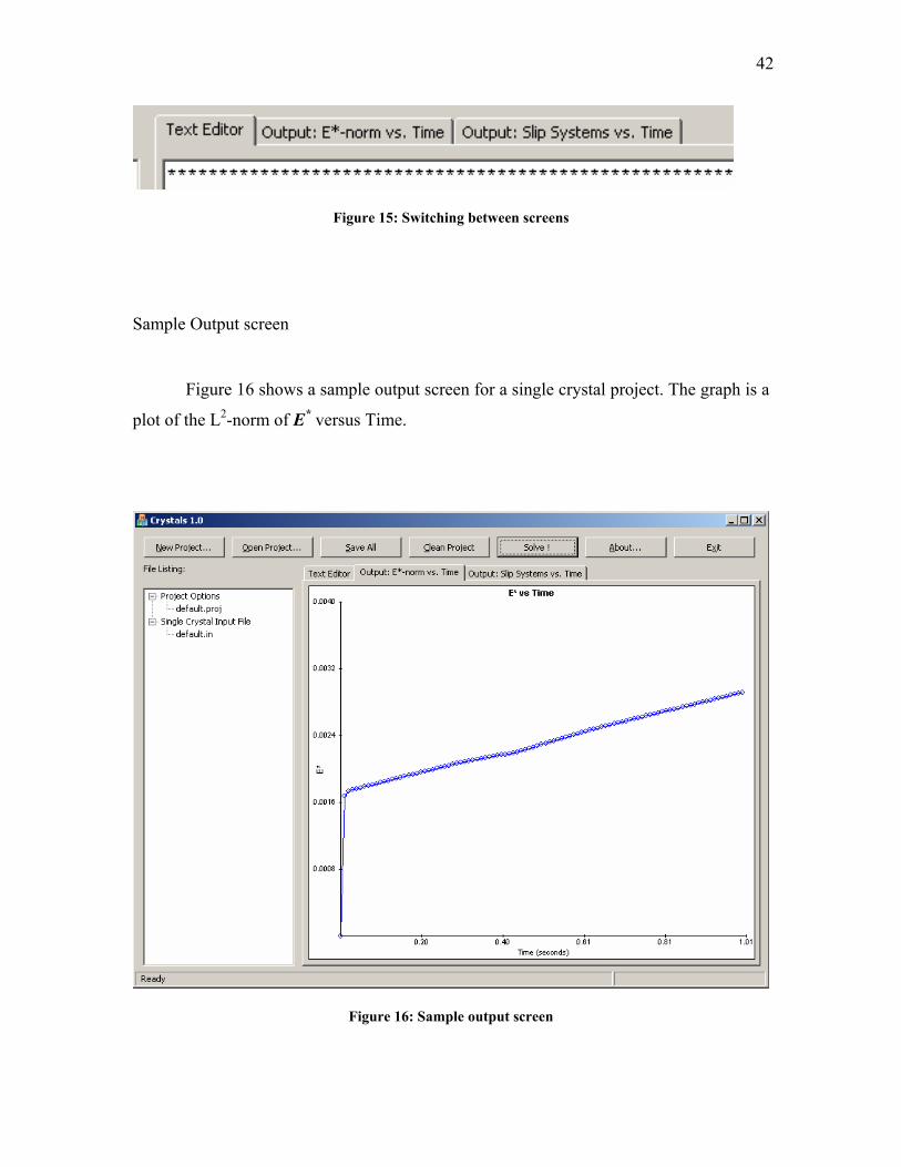
witching between screens
between the Text Editor and Output screens using the tabs at
e top of the Main window shown in Figure 15. (Note that the ordering and naming of
tabs may be different for a single crystal and polycrystal project.
S
The user can switch
th
42
Figure 15: Switching between screens
Sample Output screen
Figure 16 shows a sample output screen for a single crystal project. The graph is a * versus Time.
plot of the L2-norm of E
Figure 16: Sample output screen
43
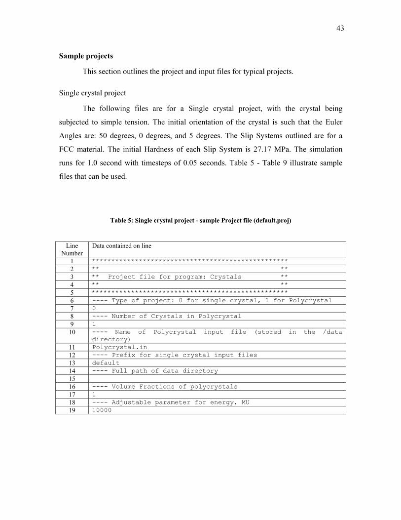
Sample projects
This section outlines the project and input files for typical projects.
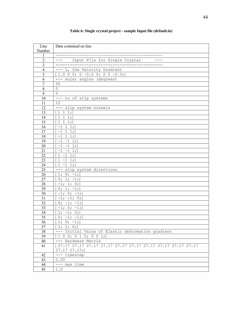
Single crystal project
The following files are for a Single crystal project, with the crystal being
subjected to simple tension. The initial orientation of the crystal is such that the Euler
Angles are: 50 degrees, 0 degrees, and 5 degrees. The Slip Systems outlined are for a
FCC material. The initial Hardness of each Slip System is 27.17 MPa. The simulation
runs for 1.0 second with timesteps of 0.05 seconds. Table 5 - Table 9 illustrate sample
files that can be used.
Table 5: Single crystal project - sample Project file (default.proj)
Line
Number Data contained on line
1 ************************************************** 2 ** ** 3 ** Project file for program: Crystals ** 4 ** ** 5 ************************************************** 6 ---- Type of project: 0 for single crystal, 1 for Polycrystal 7 0 8 ---- Number of Crystals in Polycrystal 9 1 10 ---- Name of Polycrystal input file (stored in the /data
directory) 11 Polycrystal.in 12 ---- Prefix for single crystal input files 13 default 14 ---- Full path of data directory 15 16 ---- Volume Fractions of polycrystals 17 1 18 ---- Adjustable parameter for energy, MU 19 10000
44
Table 6: Single crystal project - sample Input file (default.in)
Line
Number Data contained on line
1 --------------------------------------------- 2 --- Input File for Single Crystal --- 3 ---------------------------------------------
5 [1.0 0 0; 0 -0.5 0; 0 0 -0.5;] 6 --- euler angles (degrees) 7 50 8 0
10 --- no of slip systems 12
12 --- slip s
4 --- L, the Velocity Gradient
9 5
11 ystem normals
13 [1 1 1;] 14 [1 1 1;] 15 [1 1 1;] 16 [-1 1 1;] 17 [-1 1 1;] 18 [-1 1 1;] 19 [-1 -1 1;] 20 [-1 -1 1;] 21 [-1 -1 1;] 22 [1 -1 1;] 23 [1 -1 1;] 24 [1 -1 1;] 25 --- slip system directions 26 [1; 0; -1;] 27 [0; 1; -1;] 28 [-1; 1; 0;] 29 [0; 1; -1;] 30 [-1; 0; -1;] 31 [-1; -1; 0;] 32 [0; -1; -1;] 33 [-1; 0; -1;] 34 [1; -1; 0;] 35 [0; -1; -1;] 36 [1; 0; -1;] 37 [1; 1; 0;] 38 --- Initial Value of Elastic deformation gradient 39 [1 0 0; 0 1 0; 0 0 1;] 40 --- Hardness Matrix 41 [27.17
27.17 2 27.17 27.17 27.17 27.17 27.17 27.17 27.17 27.17 27.17 7.17;]
42 --- timestep 43 0.05 44 --- max time 45 1.0
45
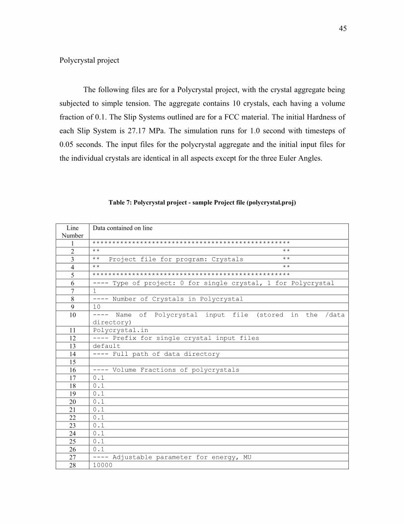
Polycrystal project
h ystal aggregate being
sub t ch having a volume
fraction f or a FCC material. The initial Hardness of
eac l runs for 1.0 second with timesteps of
0.05 seconds. The input files for the polycrystal aggregate and the initial input files for
the indi id crystals are identical in all aspects except for the three Euler Angles.
: Polycrystal project - sample Project file (polycrystal.proj)
Line
Nuon line
T e following files are for a Polycrystal project, with the cr
jec ed to simple tension. The aggregate contains 10 crystals, ea
o 0.1. The Slip Systems outlined are f
h S ip System is 27.17 MPa. The simulation
v ual
Table 7
mber Data contained
1 ************************************************** 2 ** ** 3 ** Project file for program: Crystals ** 4 ** ** 5 ************************************************** 6 ---- Type of project: 0 for single crystal, 1 for Polycrystal 7 1 8 ---- Number of Crystals in Polycrystal 9 10 10 ---- Name of Polycrystal input file (stored in the /data
directory) 11 Polycrystal.in 12 ---- Prefix for single crystal input files 13 default 14 ---- Full path of data directory 15 16 ---- Volume Fractions of polycrystals 17 0.1 18 0.1 19 0.1 20 0.1 21 0.1
0.1 23 0.1 24 0.1 25 0.1 26 0.1
22
27 ---- Adjustable parameter for energy, MU 28 10000
46
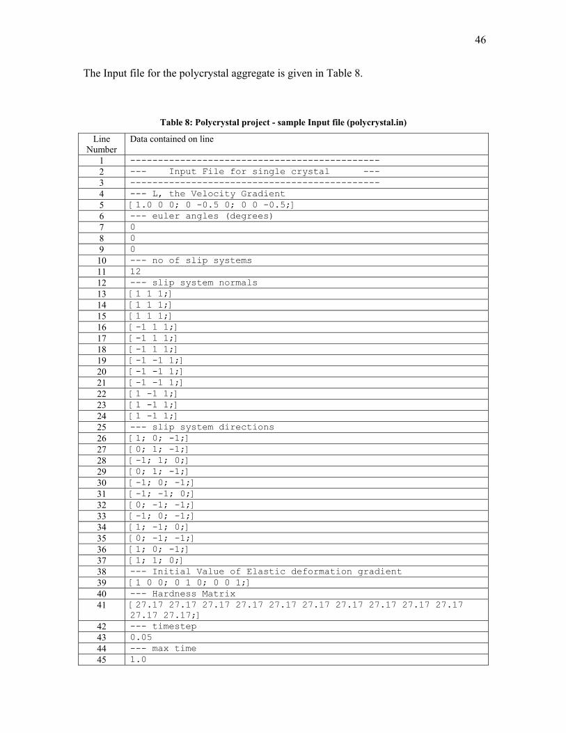
The Input file for the polycrystal aggregate is given in Table 8.
Table 8: Polycrystal project - sample Input file (polycrystal.in)
Line Number
Data contained on line
1 ---------------------------------------------
3 --------------------------------------------- --- L, the Velocity Gradient
5 [1.0 0 0; 0 -0.5 0; 0 0 -0.5;] 6 --- euler angles (degrees) 7 0
2 --- Input File for single crystal ---
4
8 0 9 0 10 --- no of slip systems
11 12 12 --- slip system normals 13 [1 1 1;] 14 [1 1 1;] 15 [1 1 1;] 16 [-1 1 1;] 17 [-1 1 1;] 18 [-1 1 1;] 19 [-1 -1 1;] 20 [-1 -1 1;] 21 [-1 -1 1;] 22 [1 -1 1;] 23 [1 -1 1;] 24 [1 -1 1;] 25 --- slip system directions 26 [1; 0; -1;]
[0; 1; -1;] 28 [-1; 1; 0;] 29 [0; 1; -1;] 30 [-1; 0; -1;] 31 [-1; -1; 0;] 32 [0; -1; -1;] 33 [-1; 0; -1;] 34 [1; -1; 0;] 35 [0; -1; -1;] 36 [1; 0; -1;] 37 [1; 1; 0;] 38 --- Initial Value of Elastic deformation gradient 39 [1 0 0; 0 1 0; 0 0 1;] 40 --- Hardness Matrix 41 [27.17 27.17 27.17 27.17 27.17 27.17 27.17 27.17 27.17 27.17
27.17;] 27.1742 --- timestep 43 0.05 44 --- max
27
time 45 1.0
47
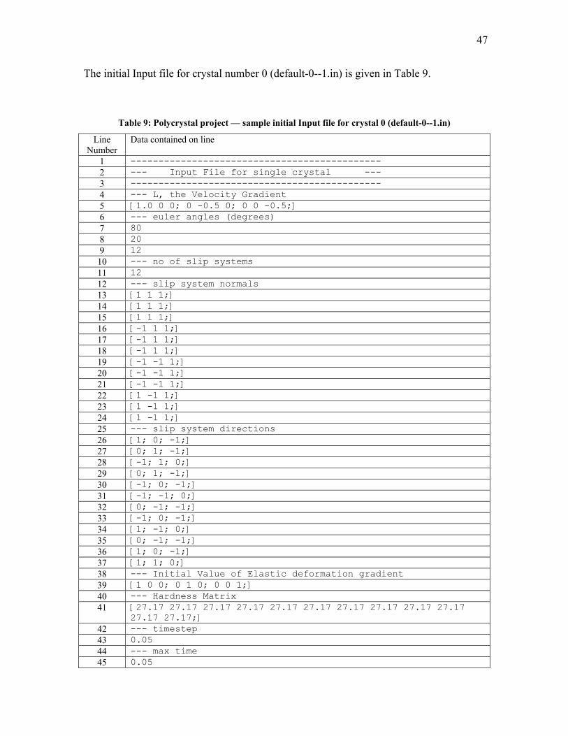
The initial Input file for crystal number 0 (default-0--1 iv.in) is g
olycrystal project — sample initial Input file for crystal 0 (defau
en in Table 9.
Table 9: P lt-0--1.in)
Line Number
Data contained on line
1 --------------------------------------------- 2 --- Input File for single crystal --- 3 --------------------------------------------- 4 --- L, the Velocity Gradient 5 [1.0 0 0; 0 -0.5 0; 0 0 -0.5;] 6 --- euler angles (degrees) 7 80 8 20 9 12 10 --- no of slip systems 11 12 12 --- slip system normals 13 [1 1 1;] 14 [1 1 1;] 15 [1 1 1;] 16 [-1 1 1;] 17 [-1 1 1;] 18 [-1 1 1;] 19 [-1 -1 1;] 20 [-1 -1 1;] 21 [-1 -1 1;] 22 [1 -1 1;] 23 [1 -1 1;] 24 [1 -1 1;] 25 --- slip system directions 26 [1; 0; -1;] 27 [0; 1; -1;] 28 [-1; 1; 0;] 29 [0; 1; -1;] 30 [-1; 0; -1;] 31 [-1; -1; 0;] 32 [0; -1; -1;] 33 [-1; 0; -1;] 34 [1; -1; 0;] 35 [0; -1; -1;] 36 [1; 0; -1;] 37 [1; 1; 0;] 38 --- Initial Value of Elastic deformation gradient 39 [1 0 0; 0 1 0; 0 0 1;] 40 --- Hardness Matrix 41 [27.17 27.17 27.17 27.17 27.17 27.17 27.17 27.17 27.17 27.17
27.17 27.17;] 42 --- timestep 43 0.05 44 --- max time 45 0.05

48
The input files for the remaining 9 crystals follow the n caming onventions
utlined earlier. The user can specify a different initial orientation for each of the
dividual crystals.
o
in
49
CHAPTER IV
RESULTS
This chapter presents the results of our simulations. First, the results of the Single
crystal solver are presented. The effect of different timesteps on the simulation is studied.
Next, a set of simulations is presented which shows the shearing rate on the individual
slip systems and the corresponding graph of strain versus time. A set of simulations is
presented which compares the difference between an empirical hardening law and the
“universal” hardening law for FCC metals. Finally, we see the difference in the graphs of
two crystals which are oriented differently with respect to the reference coordinate
system.
Single crystal simulation results
Effect of time steps
Let us consider a single FCC crystal under simple tension. The velocity gradient
for this case will be given by
The orientation of the crystal is aligned with our sample axes, i.e., the Euler
Angles are 0 deg, 0 deg and 0 deg. The slip systems are the same for all FCC materials.
The simulation is carried out for a time of 0.5 seconds.
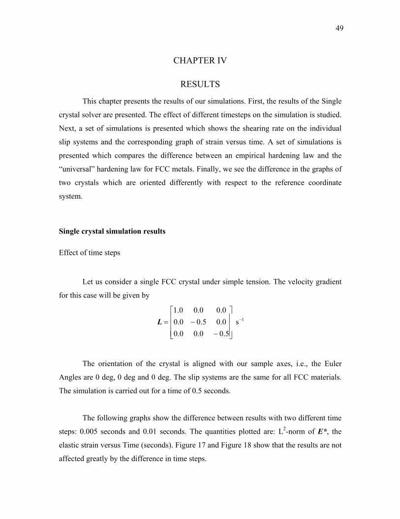
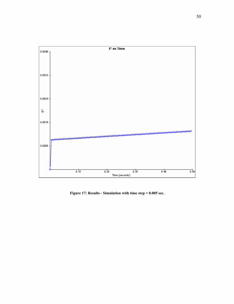
The following graphs show the difference between results with two different time
steps: 0.005 seconds and 0.01 seconds. The quantities plotted are: L2-norm of E*, the
elastic strain versus Time (seconds). Figure 17 and Figure 18 show that the results are not
affected greatly by the difference in time steps.
1s 5.00.00.0
0.05.00.00.00.00.1
−
−−=L
50
Figure 17: Results - Simulation with time step = 0.005 sec.
51
Figure 18: Results - Simula with time step = 0.01 sec. tion
52
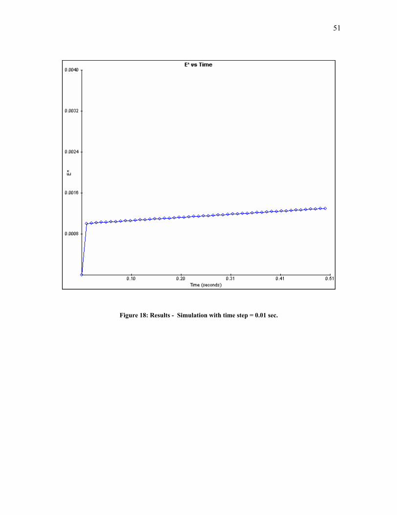
Shearing rates on slip systems
Again, consider a single FCC crystal under simple tension. The velocity gradient
for this case will be given by
The orientation of the crystal is aligned with our sample axes, i.e., the Euler
Angles are 0 deg, 0 deg and 0 deg. The slip systems are the same for all FCC materials.
The simulation is carried out for a time of 1.0 seconds. Figure 19 shows the plot of the
L2-norm of E* versus Time (seconds).
1s 5.00.00.0
0.05.00.00.00.00.1
−
−−=L
Figure 19: Results - Plot of E* vs Time
53
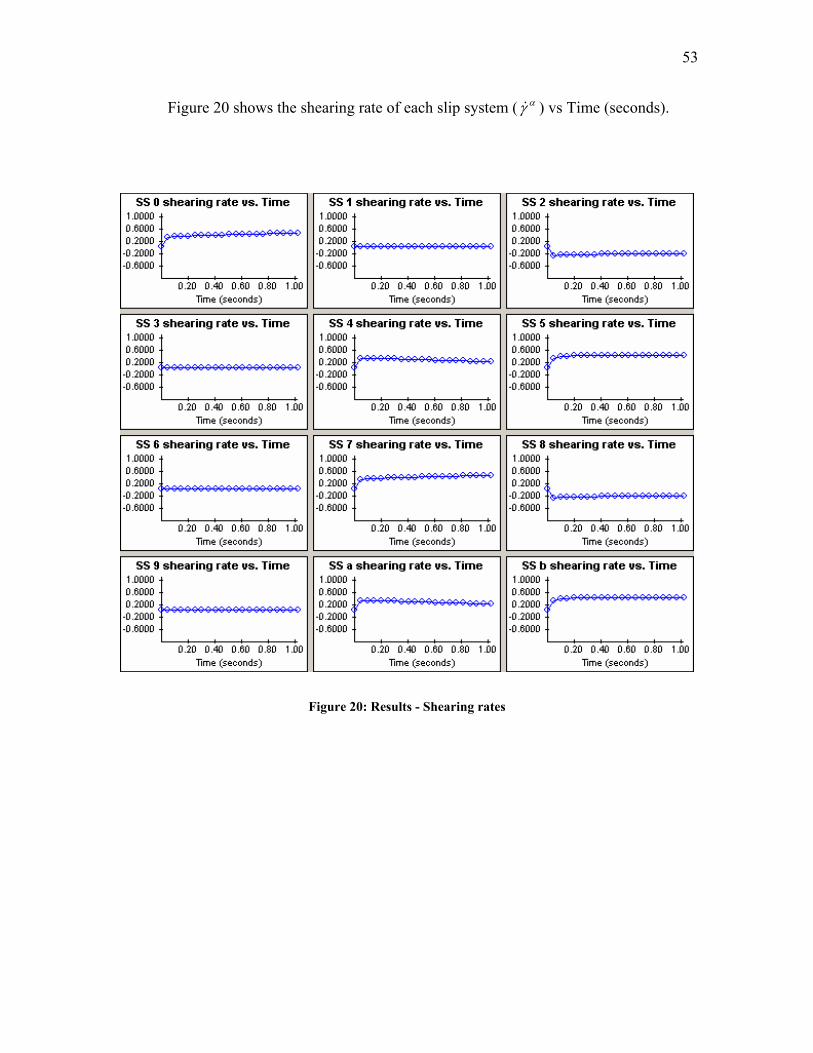
Figure 20 shows the shearing rate of each slip system ( ) vs Time (seconds).
αγ&
Figure 20: Results - Shearing rates
54
Comparison of hardening laws
Again, consider a single FCC crystal under simple tension. The velocity gradient
for this case will be given by
The orientation of the crystal is aligned with our sample axes, i.e., the Euler
Angles are 0 deg, 0 deg and 0 deg. The slip systems are the same for all FCC materials.
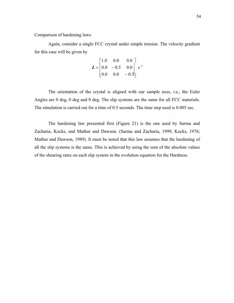
The simulation is carried out for a time of 0.5 seconds. The time step used is 0.005 sec.
The hardening law presented first (Figure 21) is the one used by Sarma and
Zacharia, Kocks, and Mathur and Dawson. (Sarma and Zacharia, 1999; Kocks, 1976;
Mathur and Dawson, 1989). It must be noted that this law assumes that the hardening of
all the slip systems is the same. This is achieved by using the sum of the absolute values
of the shearing rates on each slip system in the evolution equation for the Hardness.
1s 5.00.00.0
0.05.00.00.00.00.1
−
−−=L
55
Figure 21: Results - Old hardening law
56
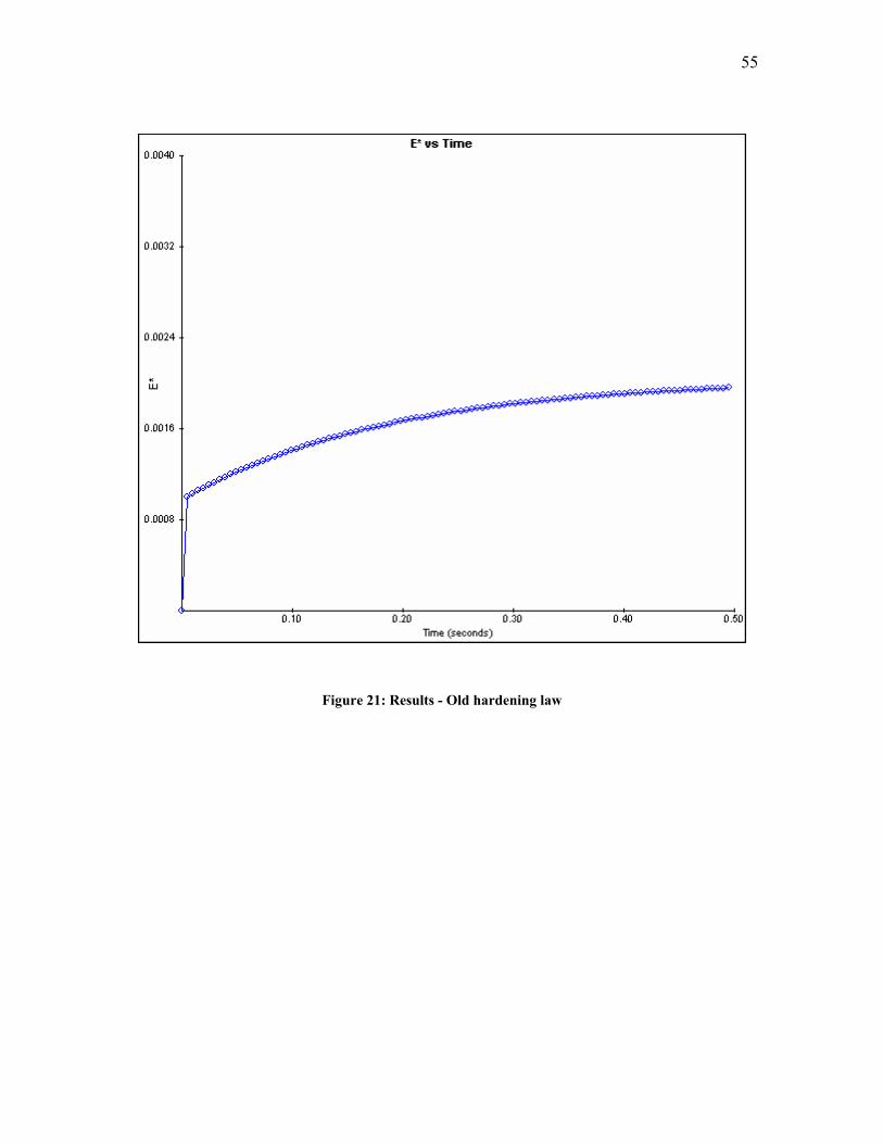
The result of using the “Universal” hardening law, is given in Figure 22.
Figure 22: Results - "Universal" FCC hardening law
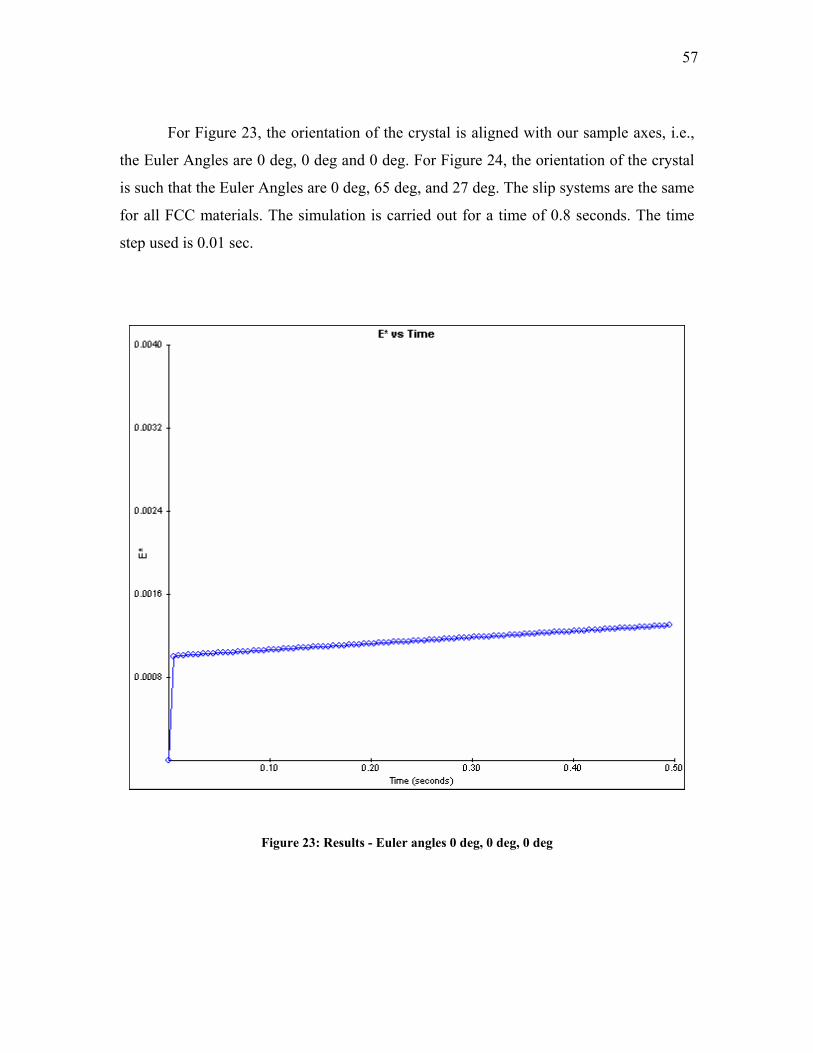
Effect of crystal orientation
Again, consider a single FCC crystal under simple tension. The velocity gradient
for this case will be given by
1s 5.00.00.0
0.05.00.00.00.00.1
−
−−=L
57
For Figure 23, the orientation of the crystal is aligned with our sample axes, i.e.,
the Euler Angles are 0 deg, 0 deg and 0 deg. For Figure 24, the orientation of the crystal
is such that the Euler Angles are 0 deg, 65 deg, and 27 deg. The slip systems are the same
for all FCC materials. The simulation is carried out for a time of 0.8 seconds. The time
step used is 0.01 sec.
Figure 23: Results - Euler angles 0 deg, 0 deg, 0 deg
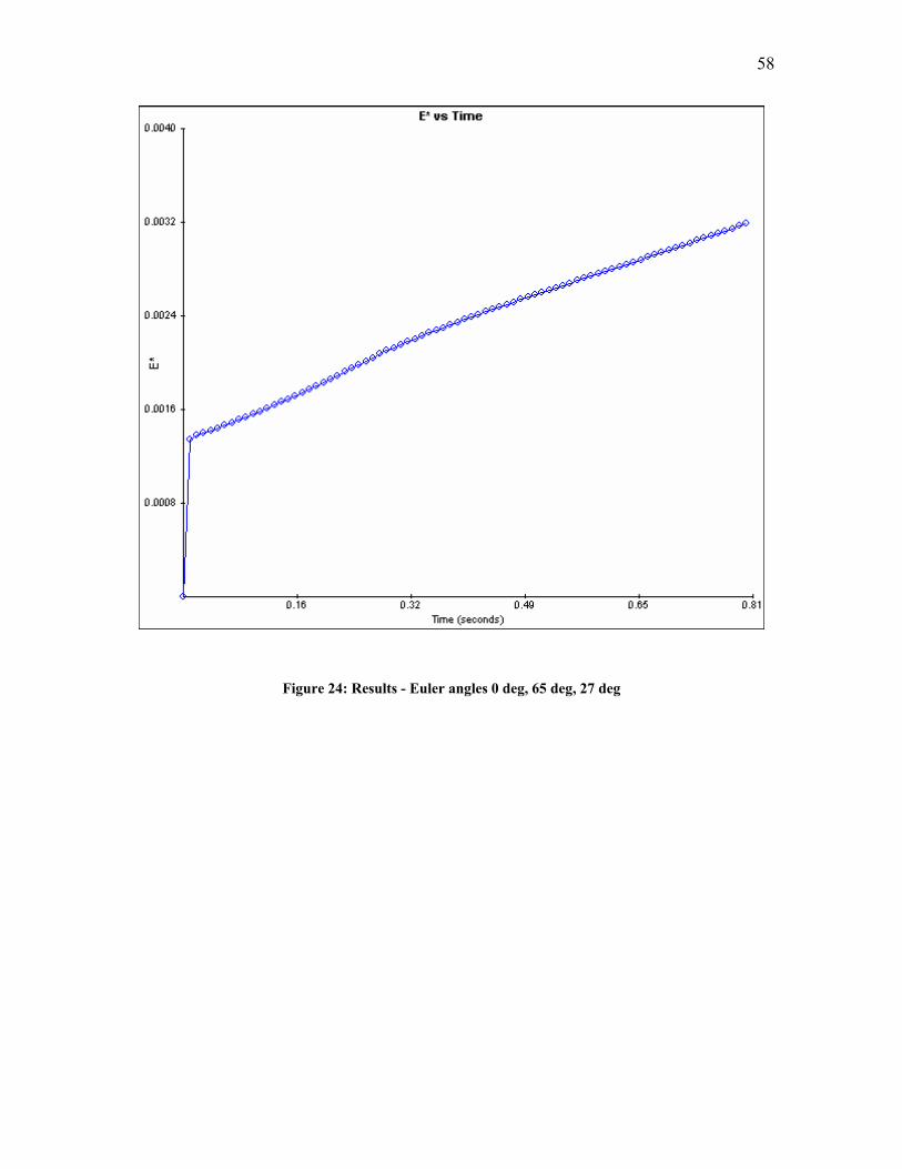
58
Figure 24: Results - Euler angles 0 deg, 65 deg, 27 deg
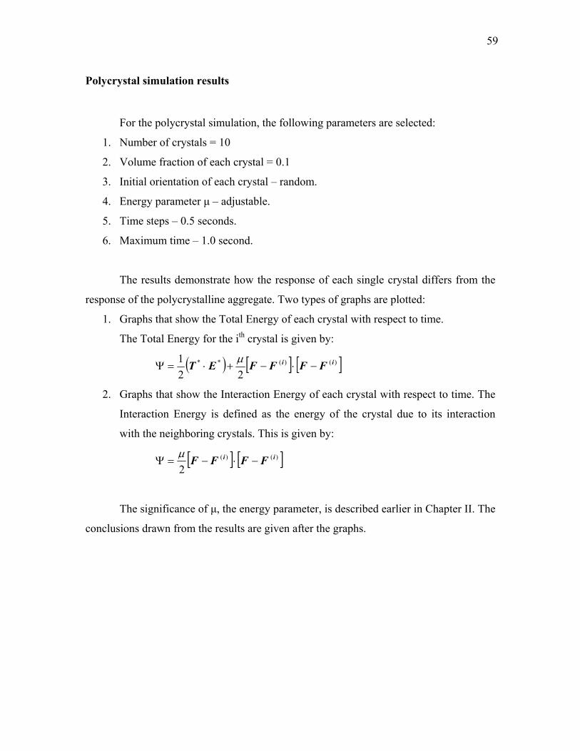
59
Polycrystal simulation results
For the polycrystal simulation, the following parameters are selected:
1. Number of crystals = 10
2. Volume fraction of each crystal = 0.1
3. Initial orientation of each crystal – random.
4. Energy parameter µ – adjustable.
5. Time steps – 0.5 seconds.
6. Maximum time – 1.0 second.
The results demonstrate how the response of each single crystal differs from the
response of the polycrystalline aggregate. Two types of graphs are plotted:
1. Graphs that show the Total Energy of each crystal with respect to time.
The Total Energy for the ith crystal is given by:
( ) [ ] [ ])()(**
221 ii FFFFET −⋅−+⋅=Ψ
µ
2. Graphs that show the Interaction Energy of each crystal with respect to time. The
Interaction Energy is defined as the energy of the crystal due to its interaction
with the neighboring crystals. This is given by:
[ ] [ ])()(
2ii FFFF −⋅−=Ψ
µ
The significance of µ, the energy parameter, is described earlier in Chapter II. The
conclusions drawn from the results are given after the graphs.
60
Two test cases are considered:
1. µ = 50 x 103 - This value is close to the Lamĕ constant for the material. Figure 25
and Figure 26 give the total energy and the interaction energy, respectively.
Figure 25: Results - total energy for µ = 50 x 103
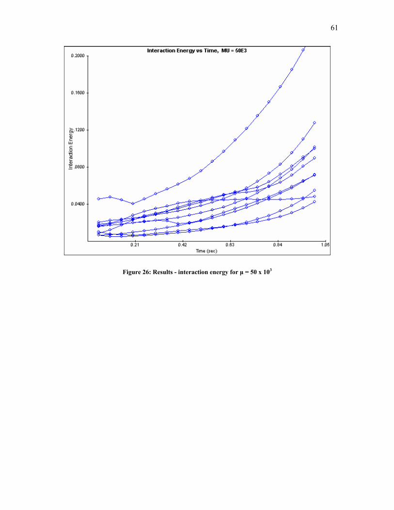
61
Figure 26: Results - interaction energy for µ = 50 x 103
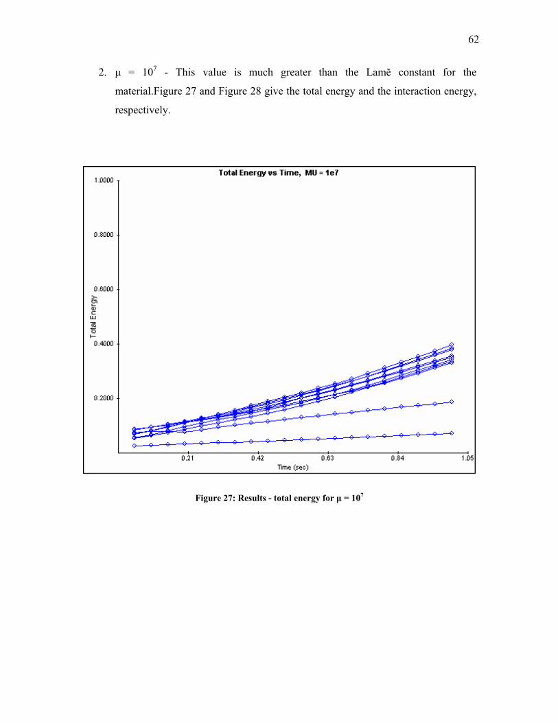
62
2. µ = 107 - This value is much greater than the Lamĕ constant for the
material.Figure 27 and Figure 28 give the total energy and the interaction energy,
respectively.
Figure 27: Results - total energy for µ = 107
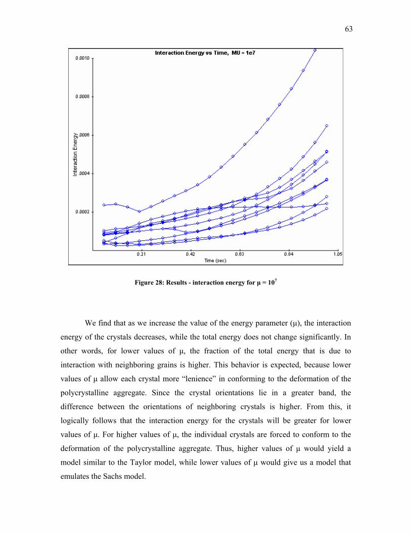
63
Figure 28: Results - interaction energy for µ = 107
We find that as we increase the value of the energy parameter (µ), the interaction
energy of the crystals decreases, while the total energy does not change significantly. In
other words, for lower values of µ, the action of the total energy that is due to
interaction with neighbo expected, because lower
values of µ allow each crystal more “lenien ” in conforming to the deformation of the
polycrystalline aggregate. Since the crystal orientations lie in a greater band, the
difference between the orientations of neighboring crystals is higher. From this, it
logically follows that the interaction energy for the crystals will be greater for lower
values of µ. For higher values of µ, the individual crystals are forced to conform to the
deformation of the polycrystalline aggregate. Thus, higher values of µ would yield a
model similar to the Taylor model, while lower values of µ would give us a model that
emulates the Sachs model.
fr
ring grains is higher. This behavior is
ce
64
CHAPTER V
CODE ORGANIZATION
The software was developed on a Microsoft Windows XP platform using C++
and Microsoft Foundation Classes. The development environment used was Microsoft
Visual Studio .NET.
Some of the general guidelines followed while writing the code were:
1. Each sub-program consists of a header file (with extension .h) and a source file
(with extension .cpp).
2. Variables follow the camel notation.
3. Member variables in a class module begin with “m_”
File listing
This section l rogram, and a broad
verview of each file. Note that the header (.h) and source code (.cpp) files are clubbed
gether as one unit. Table 10 gives the list of files used in the application.
ists the various files that constitute the p
o
to
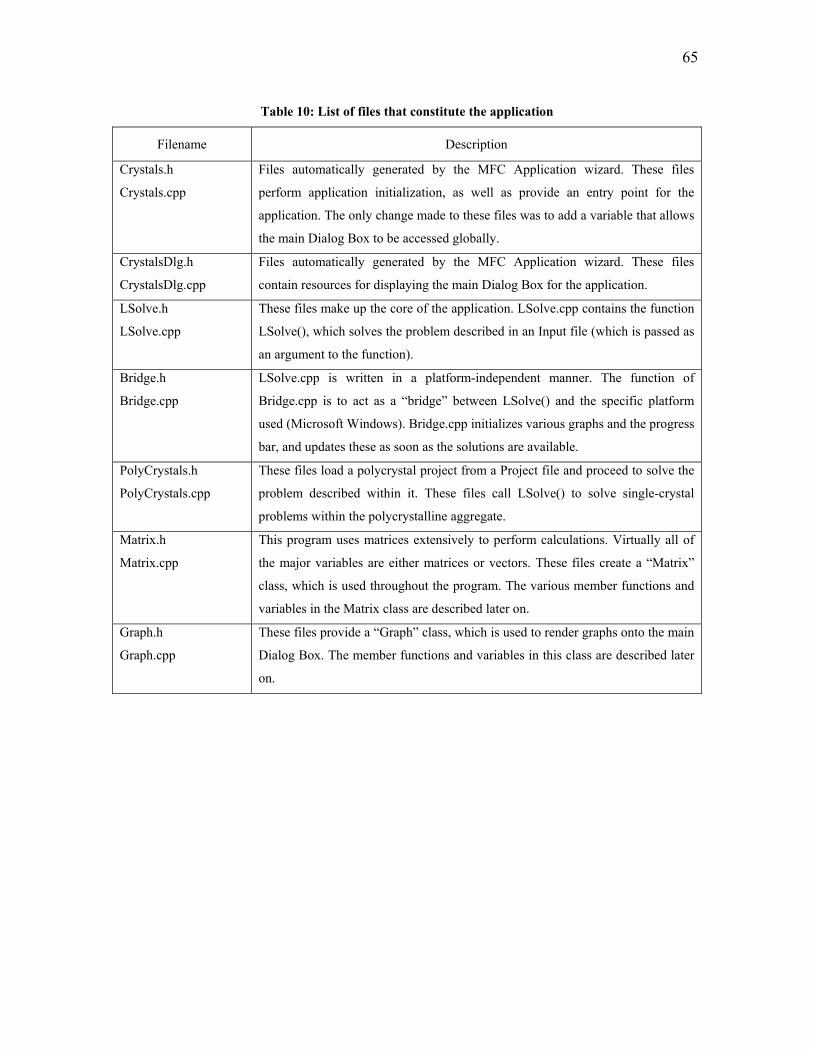
65
Table 10: List of the application
Filename
files that constitute
Description
Crystals.h
rystals.cpp
Files automatically generated by the MFC Application wizard. These files
perform application initialization, as well as provide an entry point for the C
application. The only change made to these files was to add a variable that allows
the main Dialog Box to be accessed globally.
CrystalsDlg.h
CrystalsDlg.cpp
Files automatically generated by the MFC Application wizard. These files
contain resources for displaying the main Dialog Box for the application.
LSolve.h
Solve.c
These files make up the core of the application. LSolve.cpp contains the function
h is passed as L pp LSolve(), which solves the problem described in an Input file (whic
an argument to the function).
LSolve.cpBridge.h
.c
p is written in a platform-independent manner. The function of
bridge” between LSolve() and the specific platform
used (Microsoft Windows). Bridge.cpp initializes various graphs and the progress
re available.
Bridge pp Bridge.cpp is to act as a “
bar, and updates these as soon as the solutions a
PolyCrystals.h
PolyCrystals.cpp
These files load a polycrystal project from a Project file and proceed to solve the
problem described within it. These files call LSolve() to solve single-crystal
problems within the polycrystalline aggregate.
Matrix.h
atrix.c
This program uses matrices extensively to perform calculations. Virtually all of
variables in the Matrix class are described later on.
M pp the major variables are either matrices or vectors. These files create a “Matrix”
class, which is used throughout the program. The various member functions and
Graph.h s provide a “Graph” class, which is used to render grap
Graph.cpp
hs onto the main
Dialog Box. The member functions and variables in this class are described later
on.
These file
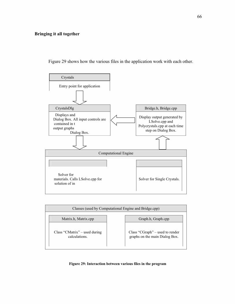
66
Bringing it all togeth
Figure 29 sho
Fi
er
ws how the various files in the application work with each other.
.h, Crystals.cpp
.h, CrystalsDlg.cpp
manages the main
his Dialog Box. All are displayed in this
LSolve.h, LSolve.cpp PolyCrystals.h, PolyCrystals.cpp
Polycrystalline
dividual crystals.
Bridge.h, Bridge.cpp
Display output generated by LSolve.cpp and
step on Dialog
Crystals
Entry point for application
CrystalsDlg
Displays andDialog Box. All input controls are contained in toutput graphs
Dialog Box.
Computational Engine
Solver for Single Crystals.
Solver formaterials. Calls LSolve.cpp for solution of in
Polycrystals.cpp at each time Box.
M
Classcal
Classes (used by Computational Engine and Bridge.cpp)
h, Matrix.cpp Graph.h, Graph.cpp
Class “
atrix.
“CMatrix” – used during
gure 29: Interaction between various file
culations. graphs
CGraph” – used to renders in the program
on the main Dialog Box.
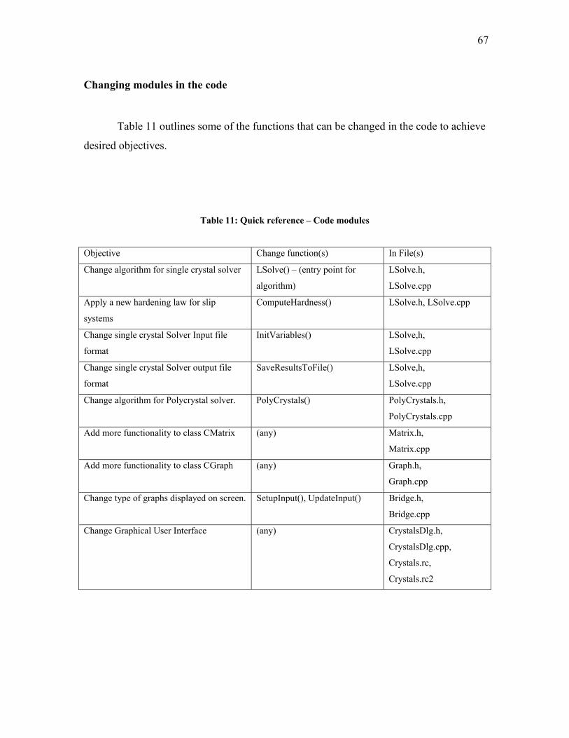
67
Changing modules in the code
Table 11 outlines some of the functions that can be changed in the code to achieve
Table 11: Quick reference – Code modules
Objective Change function(s) In File(s)
desired objectives.
Change algor LSolve() – (entry point fo
gorithm)
ithm for single crystal solver r LSolve.h,
al
hardening law for slip C
LSolve.cpp
LSolve.h, LSolvApply a new
systems
omputeHardness() e.cpp
Change single crystal Solver Input file
format
InitVariables() LSolve,h,
LSolve.cpp
Change single crystal Solver output file
format
) LSolve,h,
LSolve.cpp
SaveResultsToFile(
Change alg PolyCrystals() ls.h,
PolyCrystals.cpp
orithm for Polycrystal solver. PolyCrysta
Add more fu (any)
Matrix.cpp
nctionality to class CMatrix Matrix.h,
Add more functionality to class CGraph (any) Graph.h,
Graph.cpp
Change type of graphs displayed on screen. SetupInput(), UpdateInput() Bridge.h,
Bridge.cpp
Change Graphica (any) sDlg.h,
CrystalsDlg.cpp,
l User Interface Crystal
Crystals.rc,
Crystals.rc2
68
Classes
The code makes extensive use of Classes. There are two types of classes used in this
project.
1. Application classes: These classes are generated by the MFC Application Wizard,
and provide entry and exit points for the application. These classes are specific to
the Win32 platform.
2. Arithmetic classes: These classes are needed to perform computational tasks, such
as finding the inverse of a matrix and plotting graphs on screen.
The following classes are used in the application:
CCrystalTexturesApp
This is the application class, and is generated automatically by the MFC
Application Wizard.
CCrystalTexturesDlg
This is the Dialog class for the Crystal Textures application. The user interacts
with the application using this dialog. This class is automatically generated by the MFC
Application Wizard.
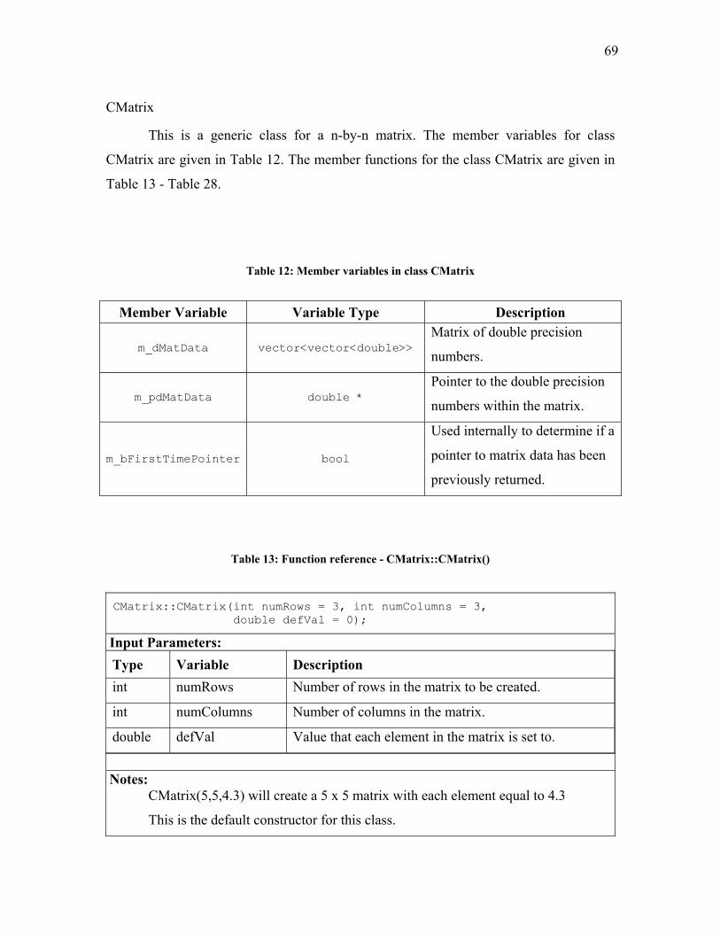
69
CMatrix
This is a generic class for a n-by-n matrix. The member variables for class
.
T
er Variable Varia tion
CMatrix are given in Table 12. The member functions for the class CMatrix are given in
Table 13 - Table 28
able 12: Member variables in class CMatrix
Memb ble Type Descrip
m_pdMatData double * Pointer to the double precision
numbers within the matrix.
m_bFirstTimePointer bool
Used inter etermine if a
pointer to matrix data has been
previously
nally to d
returned.
Table 13: Function reference - CMatrix::CMatrix()
CMatrix::CMatrix(int numRows = 3, int numColumns = 3, l
double defVa = 0);
Type Variable created.
m_dMatData vector<vector<double>>Matrix of double precision
numbers.
Input Parameters: Description
int numRows Number of rows in the matrix to be
int numColumns Number of columns in the matrix.
double defVal Value that each element in the matrix is set to. Notes: CMatrix(5,5,4.3) will create a 5 x 5 matrix with each element equal to 4.3
This is the default constructor for this class.
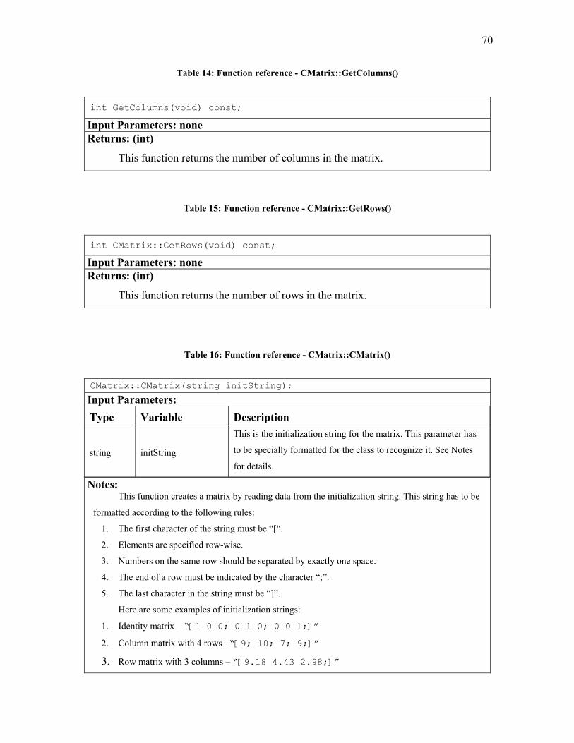
70
Table 14: Function reference - CMatrix::GetColumns()
in
t GetColumns(void) const;
Input Parameters: none Returns: (int)
This function returns the number of columns in the matrix.
Table 15: Function reference - CMatrix::GetRows()
int CMatrix::GetRows(void) const; Input Parameters: none Returns: (int)
This function returns the number of rows in the matrix.
16: Function reference - CMatrix::CMatrix() Table
CMatrix::CMatrix(string initString);
Input Parameters: Type Variable Description
string initString
This is the initialization string for the matrix. This parameter has
to be specially formatted for the class to recognize it. See Notes
for details. Notes:
This function creates a matrix by reading data from the initialization string. This string has to be
formatted according to the following rules:
1. The first character of the string must be “[“.
2. Elements are specified row-wise.
3. Numbers on the same row should be separated by exactly one space.
4. The end of a row must be indicated by the character “;”.
5. The last character in the string must be “]”.
Here are some examples of initialization strings:
1. Identity matrix – “[1 0 0; 0 1 0; 0 0 1;]”
2. Column matrix with 4 rows– “[9; 10; 7; 9;]”
3. Row matrix with 3 columns – “[9.18 4.43 2.98;]”
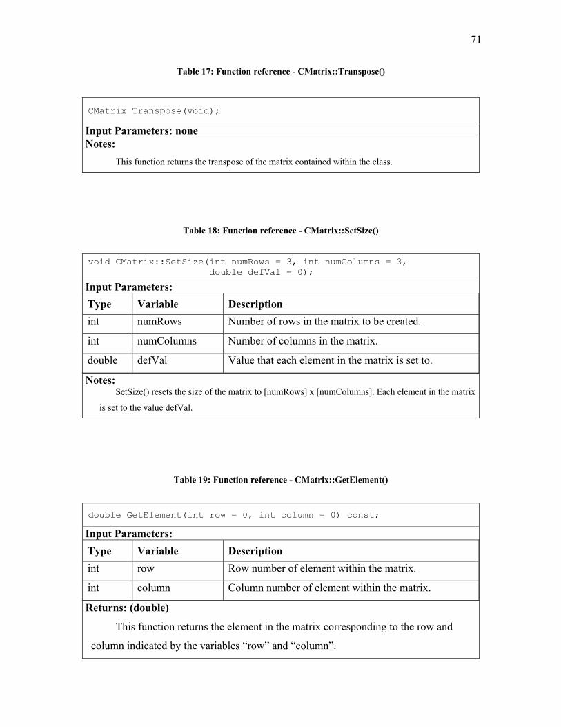
71
Table 17: Function reference - CMatrix::Transpose()
CMatrix Transpose(void);
Input Parameters: none Notes:
This function returns the transpose of the matrix contained within the class.
Table 18: Function reference - CMatrix::SetSize() void CMatrix::SetSize(int numRows = 3, int u
n double defVal = 0);
mColumns = 3,
scription atrix to be created.
he matrix.
double defVal Value that each element in the matrix is set to.
Input Parameters: Type Variable Deint numRows Number of rows in the m
int numColumns Number of columns in t
Notes:
SetSize() resets the size of the matrix to [numRows] x [numColumns]. Each element in the matrix
is set to the value defVal.
Ge int row lumn = 0) const;
Table 19: Function reference - CMatrix::GetElement()
double tElement( = 0, int co
Inpu meters: Typ Variable Description int row Row number of element within the matrix.
Returns: (double)
d
colum mn”.
This function returns the element in the matrix corresponding to the row an
n indicated by the variables “row” and “colu
t Parae
int column Column number of element within the matrix.
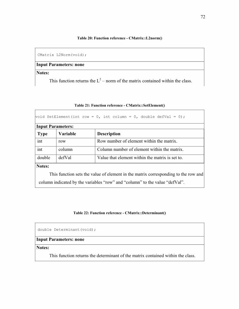
72
Table 20: Function reference - CMatrix::L2norm()
CMatrix L2Norm(void);
I Parameters: none nput
Notes:
This function returns the L2 – norm of the matrix contained within the class.
ence - CMatrix::SetElement()
t(int row = 0, int column = 0, double defVal = 0);
Table 21: Function refer
void SetElemen
Input Parameters: Type Variable Description int row Row number of element within the matrix.
int column e matrix. Column number of element within th
double defVal Value that element within the matrix is set to. Notes:
This ts the val in the matrix corresponding to the row and
column indicated by the variab
function se ue of element
les “row” and “column” to the value “defVal”.
Table 22: Function r
ut Parameters: none
tes
This function returns the determinant of th
eference - CMatrix::Determinant()
double Determinant(void);
Inp
No :
e matrix contained within the class.
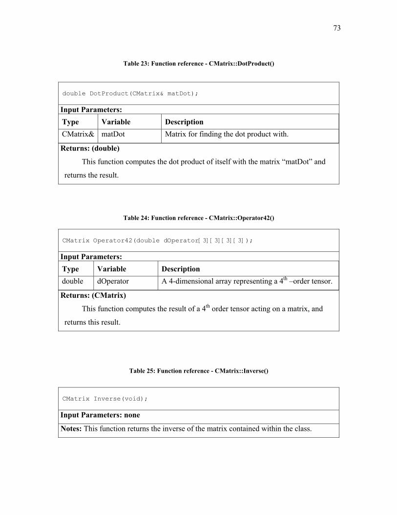
73
Table 23: Function reference - CMatrix::DotProduct()
trix& matDot);
double DotProduct(CMa
Input Parameters: Type Variable Description CMatrix& matDot Matrix for finding the dot product with.
Returns: (double)
This function c ix “matDot” and
returns the result.
omputes the dot product of itself with the matr
Table 24: Fun - CMatrix::Operator42()
trix O uble
ction reference
CMa perator42(do dOperator[3][3][3][3]);
Input Para Variable Description meters:
Type u dOperator A 4-dimensional array representing a 4th –order tensor. do ble
Returns: (CMatrix)
This function computes the result of a 4th order tensor acting on a matrix, and
returns this result.
CMatrix Inverse(void);
Table 25: Function reference - CMatrix::Inverse()
Inpu meters:
Notes: This function returns the inverse of the matrix contained within the class.
t Para none
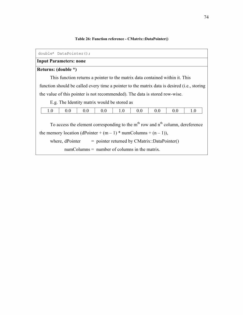
74
T ) able 26: Function reference - CMatrix::DataPointer(
double* DataPointer();
T
th th To access the element corresponding to the m row and n column, dereference
the memory location (dPointer + (m – 1) * numColumns + (n – 1)),
wher ointer = p
olumns = n
e, dP ointer returned by CMatrix::DataPointer()
numC umber of columns in the matrix.
Input Parameters: none
Returns: (double *)
his function returns a pointer to the matrix data contained within it. This
function should be called every time a pointer to the matrix data is desired (i.e., storing
the value of this pointer is not recommended). The data is stored row-wise.
E.g. The Identity matrix would be stored as
1.0 0.0 0.0 0.0 1.0 0.0 0.0 0.0 1.0
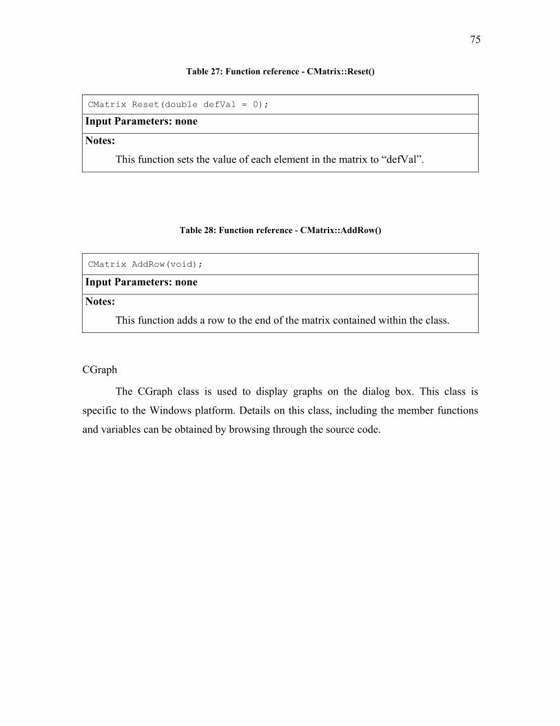
75
Table 27: Function reference - CMatrix::Reset() Matrix Reset(double defVal = 0); C
Input Parameters: none
Notes:
This function sets the value of each element in the matrix to “defVal”.
Table 28: Function reference - CMatrix::AddRow() Matrix AddRow(void); C
Input Parameters: none
Notes:
This function adds a row to the end of the matrix contained within the class.
CGraph
he ss is us s
s platform. Details on this class, including the member functions
an var
T CGraph cla ed to display graphs on the dialog box. This class i
specific to the Window
d iables can be obtained by browsing through the source code.
76
CHAPTER VI
SUMMARY AND CONCLUSION
as been set up for simulating the elastic-plastic response of single
crystal e single
cr
re ls.
e m for the single crystal solver been ted FCC tals.
Adapting it for BCC and HCP materials should involve simply changing the slip systems
in he I a
“u w allows for an
in epen
The polycrystal solver is implemented with a new theory for relating the response
f single crystals to polycrystalline aggregates. The adjustable energy parameter in this
algorithm allows us to tune the response such that it can either emulate the Taylor model,
the Sachs model, or an “intermediate” model. All output from the single crystal solver
can be stored in the form of output files on any disk. The orientation of the crystal can be
obtained from polar decomposition of the elastic deformation gradient. This data can be
used to view the development of texture in a material over time.
Future work can include integration of the predicted results with experimental
results. For example, a method can be devised to determine the texture of a material
specimen before deformation, as well as the volume fractions of the crystals that make up
the specimen. This data can be fed to the program. By comparing the experimental and
simulated results, researchers can build a database of materials and their corresponding
energy parameters. Once this database is compiled, the program can be modified such
that it will automatically select the energy parameter if the material is known.
A framework h
s as well as polycrystalline materials. Each part of the program, such as th
ystal solver and the polycrystal solver is included as a separate module. This enables
searchers to quickly test new theories for single crystals as well as polycrysta
Th odule has tes with me
t nput file passed to the solver. This module also includes an implementation of
niversal” hardening law for FCC materials. The hardening la
d dent hardening curve for each of the slip systems.
o
77
REFERENCES
Suddell, B., Herrouin, F.R.M., 2001. The effects of texture in
um alloys for engineering components under fatigue. Inter. J. Fatigue 23, S153-
S15
Bachurin, D.V., Nazarov, A.A., Shenderova, O.A., Brenner, D.W., 2003. Diffusion-
accomodated rigid-body translations along grain boundaries in nanostructured
materials. Mater. Sci. Engg. A359, 247-252.
Buerger, M.J., 1956. , Inc., New York.
anova, G. R., Fressengeas, C., Molinari, A., Kocks, U.F., 1988. Effect of rate sensitivity
d lattice rotation. Acta Metall. 8, 1961-1970.
Hertzberg, R.W., 1976. Deformation and Fracture Mechanics of Engineering Materials.
John Wiley & Sons, New York.
Hill, R., 1966. Generalized constitutive relations for incremental deformation of metal
crystals by multislip. J. Mech. Phys. Solids. 14, 95-102.
ice, J.R., 1972. Constitutive analysis of elastic-plastic crystals at arbitrary strain.
J. M
Inal, K., Wu, P.D., Neale, K.W., 2000. Simulation of earing in textured aluminum sheets.
Inter. J. Plast. 16, 635-648.
Kocks, U.F., Mecking H., 2003. Physics and phenomenology of strain hardening: the
FCC case. Progress in Mater. Sci. 48, 171-273.
Lee, E.H., 1969. Elastic-plastic deformation at finite strains. J. Appl. Mech. 36, 1-6.
Maniatty, A.M., Dawson, P.R., Lee, Y.S., 1992. A time integration algorithm for elasto-
viscoplastic cubic crystals applied to modeling polycrystalline deformation. Inter. J.
Num. Meth. Engrg 35, 1565-1588.
Mason, T.A., Maudlin, P.J., 1999. Effects of higher-order anisotropic elasticity using
textured polycrystals in three-dimensional wave propagation problems. Mech. Mater.
31, 861-882.
Bache, M.R., Evans, W.J.,
titani
9.
Elementary Crystallography. John Wiley & Sons
C
on slip system activity an
Hill, R., R
ech. Phys. Solids 20, 401-413.
Hutchinson, J.W., 1976. Bounds and self-consistent estimates for creep of polycrystalline
materials. Proc. R. Soc. Lond. A348, 101-127.
78
Mecking, H., Nicklas, B., Zarubova, N., Kocks, U.F., 1986. A “universal” temperature
scale for plastic flow. Acta Meta
Mori, T., Tanaka, K., age elastic energy of
materials with misfitting inclusions. Acta Metall. 21, 571-574.
agdhi, P.M., Srinivasa, A.R., 1993a. A dynamical theory of structured solids. I. Basic
dev
no, N., Kimura, K., Watanabe, T., 1999. Monte Carlo simulation of grain growth with
the
rate dependence and localized
deformation in crystalline solids. Acta Metall. 31, 1951-1976.
e of aluminium crystals.
Proc. R. Soc. Lond. A108, 28-51.
ll. 34, 527-535.
1973. Average stress in matrix and aver
N
elopments. Phil. Trans. R. Soc. Lond. A 345, 425-458.
Nagdhi, P.M., Srinivasa, A.R., 1993b. A dynamical theory of structured solids. I. Special
constitutive equations and special cases of the theory. Phil. Trans. R. Soc. Lond. A
345, 459-476.
O
full spectra of grain orientation and grain boundary energy. Acta Mater. 47, 1007-
1017.
Pan, J., Rice, J.R., 1983. Rate sensitivity of plastic flow and implications for yield surface
vertices. Int. J. Solids Struct. 19, 973-987.
Peirce, D., Asaro, R.J., Needleman, A., 1983. Material
Rice, J.R., 1971. Inelastic constitutive relations for solids: an internal-variable theory and
its application to metal plasticity. J. Mech. Phys. Solids 19, 433-455.
Rollett, A.D., Storch, M.L., Hilsinki, E.J., Goodman, S.R., 2001. Approach to saturation
in textured soft magnetic materials. Metall. Mater. Trans. A 32, 2595-2603.
Sarma, G., Zacharia, T., 1999. Integration algorithm for modeling the elasto-viscoplastic
response of polycrystalline materials. J. Mech. Phys. Solids 47, 1219-1238.
Taylor, G.I., Elam, C.F., 1925. The plastic extension and fractur
Taylor, G.I., 1938. Plastic strain in metals. J. Inst. Metals 62, 307-324.
Van Houtte, P., Delannay, L., Kalidindi, S.R., 2002. Comparison of two grain interaction
models for polycrystal plasticity and deformation texture prediction. Inter. J. Plast. 18,
359-377.
Yuan, W.Q., Wang, J.N., 2002. Anisotropy of the phase-transformation plasticity in
textured CuZnAl shape-memory sheets. J. Mater. Proc. Tech. 123, 31-35.
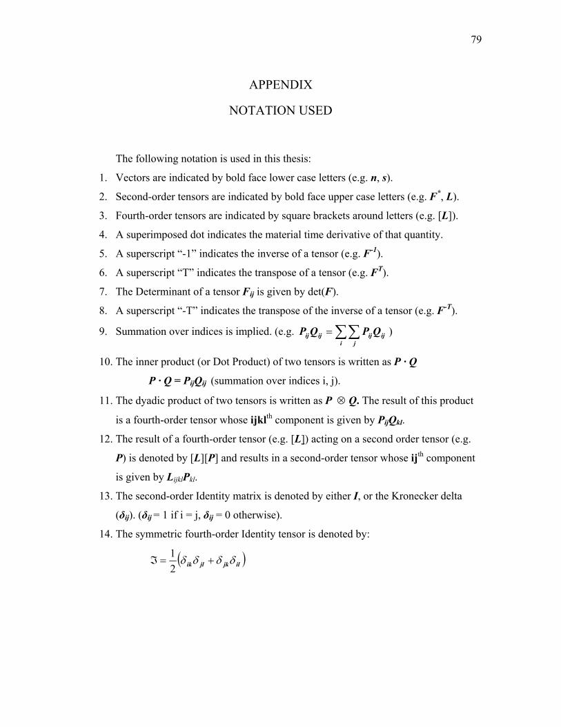
79
APPENDIX
NOTATION USED
following notation is used in this thesis:
re brackets around letters (e.g. [L]).
he transpose of the inverse of a tensor (e.g. F-T).
The
1. Vectors are indicated by bold face lower case letters (e.g. n, s).
2. Second-order tensors are indicated by bold face upper case letters (e.g. F*, L).
3. Fourth-order tensors are indicated by squa
4. A superimposed dot indicates the material time derivative of that quantity.
5. A superscript “-1” indicates the inverse of a tensor (e.g. F-1).
6. A superscript “T” indicates the transpose of a tensor (e.g. FT).
7. The Determinant of a tensor Fij is given by det(F).
8. A superscript “-T” indicates t
9. Summation over indices is implied. (e.g. ∑∑=i
ijijijij QPQP ) j
10. The inner product (or Dot Product) of two tensors is written as P · Q
P · Q = PijQij n over indices i, j).
th ent is given by PijQkl.
(summatio
11. The dyadic product of two tensors is written as P ⊗ Q. The result of this product
is a fourth-order tensor whose ijkl compon
12. The result of a fourth-order tensor (e.g. [L]) acting on a second order tensor (e.g.
P) is denoted by [L][P] and results in a second-order tensor whose ijth component
by either I, or the Kronecker delta
is given by LijklPkl.
13. The second-order Identity matrix is denoted
(δij). (δij = 1 if i = j, δij = 0 otherwise).
14. The symmetric fourth-order Identity tensor is denoted by:
( )iljkjlik δδδδ +=ℑ1 2
80
VITA
Parag Vilas Patwardhan obtained his Bachelor of Engineering degree in mechanical
eng e – India. In the Fall of
Texas A&M University and received it in December 2003.
Parag Vilas Patwardhan
Ban
Pune – 411007
ineering from the Government College of Engineering, Pun
2001, he began studying for his Master of Science degree in mechanical engineering at
3, Vibha Heights, Sane Wadi,
er Road, Aundh,
Maharashtra, India.
Top Related