


Languages
Pages
Legal

Modeling naturalistic affective states via facial and vo-
cal expressions recognition George Caridakis1, Lori Malatesta1, Loic Kessous2, Noam Amir2,
Amaryllis Raouzaiou1 and Kostas Karpouzis1
1 School of Electrical and Computer Engineering, National Technical University of Athens, Politechnioupoli, Zographou, Greece
{gcari, lori, araouz, kkarpou }@image.ece.ntua.gr 2Tel Aviv Academic College of Engineering
218 Bnei Efraim St. 69107, Tel Aviv, Israel
[email protected], [email protected]
ABSTRACT
Affective and human-centered computing are two areas related to
HCI which have attracted attention during the past years. One of
the reasons that this may be attributed to, is the plethora of devic-
es able to record and process multimodal input from the part of
the users and adapt their functionality to their preferences or indi-
vidual habits, thus enhancing usability and becoming attractive to
users less accustomed with conventional interfaces. In the quest to
receive feedback from the users in an unobtrusive manner, the
visual and auditory modalities allow us to infer the users’ emo-
tional state, combining information both from facial expression
recognition and speech prosody feature extraction. In this paper,
we describe a multi-cue, dynamic approach in naturalistic video
sequences. Contrary to strictly controlled recording conditions of
audiovisual material, the current research focuses on sequences
taken from nearly real world situations. Recognition is performed
via a ‘Simple Recurrent Network’ which lends itself well to mod-
eling dynamic events in both user’s facial expressions and speech.
Moreover this approach differs from existing work in that it mod-
els user expressivity using a dimensional representation of activa-
tion and valence, instead of detecting the usual ‘universal emo-
tions’ which are scarce in everyday human-machine interaction.
The algorithm is deployed on an audiovisual database which was
recorded simulating human-human discourse and, therefore, con-
tains less extreme expressivity and subtle variations of a number
of emotion labels.
Categories and Subject Descriptors
H.5.2 [Information Interfaces and Presentation]: User Interfac-
es – User-centered design, interaction styles, standardization.
Keywords
Affective interaction, multimodal analysis, image processing,
facial expression recognition, user modeling, prosodic feature
extraction, naturalistic data.
1. INTRODUCTION The introduction of the term ‘affective computing’ by R. Picard 7
epitomizes the fact that computing is no longer considered a
‘number crunching’ discipline, but should be thought of as an
interfacing means between humans and machines and sometimes
even between humans alone. To achieve this, application design
must take into account the ability of humans to provide multi-
modal input to computers, thus moving away from the monolithic
window-mouse-pointer interface paradigm and utilizing more
intuitive concepts, closer to human niches ([2], [3]). A large part
of this naturalistic interaction concept is expressivity [4], both in
terms of interpreting the reaction of the user to a particular event
or taking into account their emotional state and adapting presenta-
tion to it, since it alleviates the learning curve for conventional
interfaces and makes less technology-savvy users feel more com-
fortable. In this framework, both speech and facial expressions are
of great importance, since they usually provide a comprehensible
view of users’ reactions.
The complexity of the problem relies in the combination of the
information extracted from modalities, the interpretation of the
data through time and the noise alleviation from the natural set-
ting. The current work aims to interpret sequences of events thus
modeling the user’s behaviour through time. With the use of a
recurrent neural network, the short term memory, provided
through its feedback connection, works as a memory buffer and
the information remembered is taken under consideration in every
next time cycle. Theory on this kind of network back up the claim
that it is suitable for learning to recognize and generate temporal
patterns as well as spatial ones [10].
The naturalistic data chosen as input is closer to human reality
since the dialogues are not acted, and the expressivity is not guid-
ed by directives (e.g. Neutral expression one of the six univer-
sal emotions neutral). This amplifies the difficulty in discern-
ing facial expressions and speech patterns. Nevertheless it pro-
vides the perfect test-bed for the combination of the conclusions
drawn from each modality in one time unit and use as input in the
following sequence of audio and visual events analysed.
Permission to make digital or hard copies of all or part of this work for
personal or classroom use is granted without fee provided that copies are
not made or distributed for profit or commercial advantage and that
copies bear this notice and the full citation on the first page. To copy
otherwise, or republish, to post on servers or to redistribute to lists,
requires prior specific permission and/or a fee.
Conference’04, Month 1–2, 2004, City, State, Country.
Copyright 2004 ACM 1-58113-000-0/00/0004…$5.00.
2. DATA COLLECTION Research on signs of emotion emerged as a technical field around
1975, with research by Ekman and his colleagues [36] on encod-
ing emotion-related features of facial expression, and by Williams
and Stevens [37] on emotion in the voice. The early paradigms
simplified their task by concentrating on emotional extremes –
often simulated, and not always by skilled actors. Most of the data
used in research on speech and emotion has three characteristics:
the emotion in it is simulated by an actor (not necessarily trained);
the actor is reading preset material; and he or she is aiming to
simulate fullblown emotion.
That kind of material has obvious attractions: it is easy to obtain,
and it lends itself to controlled studies. However, it has become
reasonably clear that it does not do a great deal to illuminate the
way face and speech express emotion in natural settings. The
1990’s saw growing interest in naturalistic data, but retained a
focus on cases where emotion was at or approaching an extreme.
The major alternative is to develop techniques which might be
called directed elicitation – techniques designed to induce states
that are both genuinely emotional and likely to involve speech.
Most of these tasks have a restricted range. They provide more
control and higher data rates than other methods, but they still
tend to elicit weak negative emotions, and they often impose con-
straints on the linguistic form and content of the speech which
may restrict generalisation. One of them, SAL, was used to ac-
quire the data processed by the presented system.
The SAL scenario [42] is a development of the ELIZA concept
introduced by Weizenbaum. The user communicates with a sys-
tem whose responses give the impression of sympathetic under-
standing, and that allows a sustained interaction to build up. In
fact, though, the system takes no account of the user’s meaning: it
simply picks from a repertoire of stock responses on the basis of
surface cues extracted from the user’s contributions. A second
factor in the selection is that the user selects one of four ‘artificial
listeners’ to interact with at any given time. Each one will try to
initiate discussion by providing cues mapped to each of the four
quadrants defined by valence and activation – ‘Spike’ is provoca-
tive or angry (negative/active), while ‘Poppy’ is always happy
(positive/active). SAL took its present form as a result of a good
deal of pilot work [27]. In that form, it provides a framework
within which users do express a considerable range of emotions in
ways that are virtually unconstrained. The process depends on
users’ co-operation – they are told that it is like an emotional gym,
and they have to use the machinery it provides to exercise their
emotions. But if they do enter into the spirit, they can move
through a very considerable emotional range in a recording ses-
sion or a series of recording sessions: the ‘artificial listeners’ are
designed to let them do exactly that.
As far as emotion representation is concerned we use the Activa-
tion-Evaluation space. Activation-Evaluation space as a represen-
tation has great appeal as it is both simple, while at the same time
makes it possible to capture a wide range of significant issues in
emotion. The concept is based on a simplified treatment of two
key themes:
- Valence: The clearest common element of emotional states
is that the person is materially influenced by feelings that
are valenced, i.e., they are centrally concerned with positive
or negative evaluations of people or things or events.
- Activation level: Research from Darwin forward has recog-
nized that emotional states involve dispositions to act in cer-
tain ways. A basic way of reflecting that theme turns out to
be surprisingly useful. States are simply rated in terms of the
associated activation level, i.e., the strength of the person’s
disposition to take some action rather than none.
Dimensional representations are attractive mainly because they
provide a way of describing emotional states that is more tractable
than using words. This is of particular importance when dealing
with naturalistic data, where a wide range of emotional states
occur. Similarly, they are much more able to deal with
non-discrete emotions and variations in emotional state over time,
since it such cases changing from one universal emotion label to
another would not make much sense in real life scenarios.
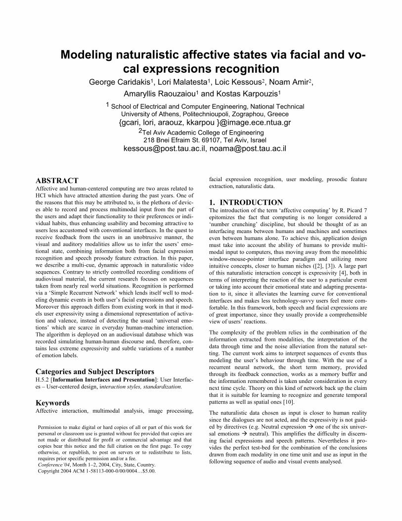
The available SAL Data Set is given along with some of their
important features in Table 1, while Figure 1 shows some frames
of the processed naturalistic data.
Table 1. Summary of the available SAL data sets up to date.
Data Set
Subjects 2 males, 2 females
Passages 76
Tunes ~1600
Emotion space coverage Yes, all quadrants
FeelTrace ratings 4 rators
Transcripts Yes
Text Post-Processing No
Figure 1. Frames of SAL dataset
Naturalistic data goes beyond extreme emotions, as is usually the
case in existing approaches, and concentrates on more natural
emotional episodes that happen more frequently in everyday dis-
course, that’s why the output of the presented system is not a well
known emotion, but a quadrant of the Activation-Evaluation
space.
3. FACIAL FEATURES EXTRACTION
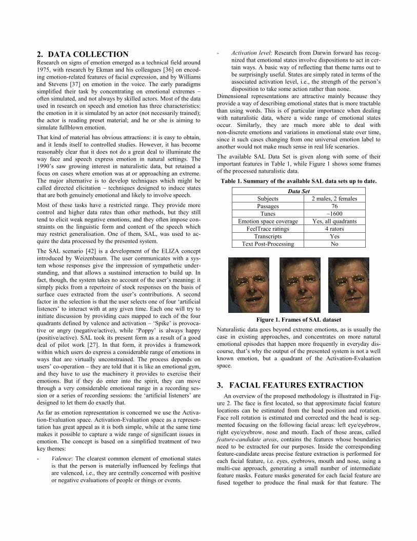
An overview of the proposed methodology is illustrated in Fig-
ure 2. The face is first located, so that approximate facial feature
locations can be estimated from the head position and rotation.
Face roll rotation is estimated and corrected and the head is seg-
mented focusing on the following facial areas: left eye/eyebrow,
right eye/eyebrow, nose and mouth. Each of those areas, called
feature-candidate areas, contains the features whose boundaries
need to be extracted for our purposes. Inside the corresponding
feature-candidate areas precise feature extraction is performed for
each facial feature, i.e. eyes, eyebrows, mouth and nose, using a
multi-cue approach, generating a small number of intermediate
feature masks. Feature masks generated for each facial feature are
fused together to produce the final mask for that feature. The
mask fusion process uses anthropometric criteria [29] to perform
validation and weight assignment on each intermediate mask;
each feature’s weighted masks are then fused to produce a final
mask along with confidence level estimation.
Figure 2. Diagram of the proposed methodology
Since this procedure essentially locates and tracks points in the
facial area, we chose to work with MPEG-4 FAPs and not Action
Units (AUs), since the former are explicitly defined to measure
the deformation of these feature points. In addition to this, dis-
crete points are easier to track in cases of extreme rotations and
their position can be estimated based on anthropometry in cases of
occlusion, whereas this is not usually the case with whole facial
features. Another feature of FAPs which proved useful is their
value (or magnitude) which is crucial in order to differentiate
cases of varying activation of the same emotion (e.g. joy and ex-
hilaration) [34] and exploit fuzziness in rule-based systems [13].
Measurement of Facial Animation Parameters (FAPs) requires the
availability of a frame where the subject’s expression is found to
be neutral. This frame will be called the neutral frame and is
manually selected from video sequences to be analyzed or interac-
tively provided to the system when initially brought into a specific
user’s ownership. The final feature masks are used to extract 19
Feature Points (FPs) [34]; Feature Points obtained from each
frame are compared to FPs obtained from the neutral frame to
estimate facial deformations and produce the Facial Animation
Parameters (FAPs). Confidence levels on FAP estimation are
derived from the equivalent feature point confidence levels. The
FAPs are used along with their confidence levels to provide the
facial expression estimation.
3.1 Face Detection and Pose Estimation
In the proposed approach facial features including eyebrows,
eyes, mouth and nose are first detected and localized. Thus, a first
processing step of face detection and pose estimation is carried
out as described below, to be followed by the actual facial feature
extraction process described in section 3.2. At this stage, it is
assumed that an image of the user at neutral expression is availa-
ble, either a-priori, or captured before interaction with the pro-
posed system starts.
The goal of face detection is to determine whether or not there
are faces in the image, and if yes, return the image location and
extent of each face [35]. Face detection can be performed with a
variety of methods. In this paper we used nonparametric discrimi-
nant analysis with a Support Vector Machine (SVM) which classi-
fies face and non-face areas reducing the training problem dimen-
sion to a fraction of the original with negligible loss of classifica-
tion performance [30],[27].
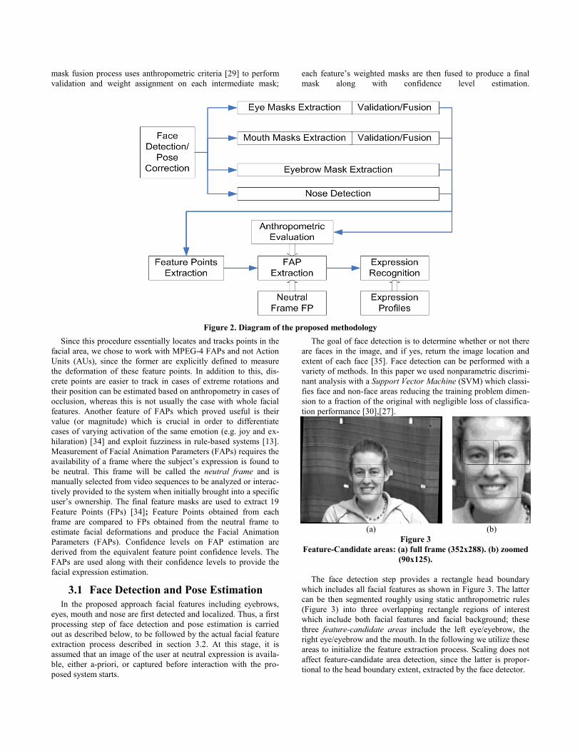
(a) (b)
Figure 3
Feature-Candidate areas: (a) full frame (352x288). (b) zoomed
(90x125).
The face detection step provides a rectangle head boundary
which includes all facial features as shown in Figure 3. The latter
can be then segmented roughly using static anthropometric rules
(Figure 3) into three overlapping rectangle regions of interest
which include both facial features and facial background; these
three feature-candidate areas include the left eye/eyebrow, the
right eye/eyebrow and the mouth. In the following we utilize these
areas to initialize the feature extraction process. Scaling does not
affect feature-candidate area detection, since the latter is propor-
tional to the head boundary extent, extracted by the face detector.

The accuracy of feature extraction depends on head pose. In
this paper we are mainly concerned with roll rotation, since it is
the most frequent rotation encountered in real life video sequenc-
es. Small head yaw and pitch rotations which do not lead to fea-
ture occlusion do not have a significant impact on facial expres-
sion recognition. The face detection techniques described in the
former section is able to cope with head roll rotations up to 30o.
This is a quite satisfactory range in which the feature-candidate
areas are large enough so that the eyes reside in the eye-candidate
search areas defined by the initial segmentation of a rotated face.
To estimate the head pose we first locate the left and right eyes
in the detected corresponding eye candidate areas. After locating
the eyes, we can estimate head roll rotation by calculating the
angle between the horizontal plane and the line defined by the eye
centers. To increase speed and reduce memory requirements, the
eyes are not detected on every frame using the neural network.
Instead, after the eyes are located in the first frame, two square
grayscale eye templates are created, containing each of the eyes
and a small area around them. The size of the templates is half the
eye-center distance (bipupil breadth, Dbp). For the following
frames, the eyes are located inside the two eye-candidate areas,
using template matching which is performed by finding the loca-
tion where the sum of absolute differences (SAD) is minimized.
After head pose is computed, the head is rotated to an upright
position and new feature-candidate segmentation is performed on
the head using the same rules so as to ensure facial features reside
inside their respective candidate regions. These regions containing
the facial features are used as input for the facial feature extraction
stage, described in the following section.
3.2 Automatic Facial Feature Detection
and Boundary Extraction
To be able to compute MPEG-4 FAPs, precise feature bounda-
ries for the eyes, eyebrows and mouth have to be extracted. Eye
boundary detection is usually performed by detecting the special
color characteristics of the eye area [26], by using luminance pro-
jections, reverse skin probabilities or eye model fitting. Mouth
boundary detection in the case of a closed mouth is a relatively
easily accomplished task. In case of an open mouth, several meth-
ods have been proposed which make use of intensity or color
information [26]. Color estimation is very sensitive to environ-
mental conditions, such as lighting or capturing camera’s charac-
teristics and precision. Model fitting usually depends on ellipse or
circle fitting, using Hough-like voting or corner detection [31].
Those techniques while providing accurate results in high resolu-
tion images, are unable to perform well with low video resolution
which lack high frequency properties; such properties which are
essential for efficient corner detection and feature border
trackability [32], are usually lost due to analogue video media
transcoding or low quality digital video compression.
In this work, nose detection and eyebrow mask extraction are
performed in a single stage, while for eyes and mouth which are
more difficult to handle, multiple (four in our case) masks are
created taking advantage of our knowledge about different proper-
ties of the feature area; the latter are then combined to provide the
final estimates as shown in Figure 4. More technical details can be
found at [13].
3.2.1 Eye Boundary Detection
Luminance and color information fusion mask tries to refine
eye boundaries extracted by the neural network described earlier
building on the fact that eyelids usually appear darker than skin
due to eyelashes and are almost always adjacent to the iris. The
initial mask provided by the neural network is thresholded and the
distance transformation of the resulting mask gives as the first eye
mask.
This second approach is based on eyelid edge detection. Eye-
lids reside above and below the eye centre, which has already
been estimated by the neural network. Taking advantage of their
mainly horizontal orientation, eyelids are easily located through
edge detection. By combining the canny edge detector and the
vertical gradient we are locating the eyelids and the space between
them is considered the eye mask.
A third mask is created for each of the eyes to strengthen the
final mask fusion stage. This mask is created using a region grow-
ing technique; the latter usually gives very good segmentation
results corresponding well to the observed edges. Construction of
this mask relies on the fact that facial texture is more complex and
darker inside the eye area and especially in the eyelid-sclera-iris
borders, than in the areas around them. Instead of using an edge
density criterion, we developed a simple but effective iterative
method to estimate both the eye centre and eye mask based on the
standard deviation of the luminance channel.
Finally, a second luminance-based mask is constructed for
eye/eyelid border extraction. In this mask, we compute the normal
luminance probability resembling to the mean luminance value of
eye area defined by the NN mask. From the resulting probability
mask, the areas with a given confidence interval are selected and
small gaps are closed with morphological filtering. The result is
usually a blob depicting the boundaries of the eye. In some cases,
the luminance values around the eye are very low due to shadows
from the eyebrows and the upper part of the nose. To improve the
outcome in such cases, the detected blob is cut vertically at its
thinnest points from both sides of the eye centre; the resulting
mask’s convex hull is used as the Luminance mask (Figure 4).
(a) (b) (c)
Figure 4. Eye masks
3.2.2 Eyebrow Boundary Detection
Eyebrows are extracted based on the fact that they have a sim-
ple directional shape and that they are located on the forehead,
which due to its protrusion, has a mostly uniform illumination.
Each of the left and right eye and eyebrow-candidate images
shown in Figure 3 is used for brow mask construction.
The first step in eyebrow detection is the construction of an
edge map of the grayscale eye/eyebrow-candidate image. This
map is constructed by subtracting the dilation and erosion of the
grayscale image using a line structuring element of size n and then
thresholding the result. The selected edge detection mechanism is
appropriate for eyebrows because it can be directional; it pre-
serves the feature’s original size and can be combined with a
threshold to remove smaller skin anomalies such as wrinkles. The
above procedure can be considered as a non-linear high-pass fil-
ter.
Each connected component on the edge map is labeled and
then tested against a set of filtering criteria. These criteria were
formed through statistical analysis of the eyebrow lengths and
positions on 20 persons of the ERMIS database [27]. Firstly, the
major axis is found for each component through principal compo-
nent analysis (PCA). All components whose major axis has an
angle of more than 30 degrees with the horizontal plane are re-
moved from the set. From the remaining components, those whose
axis length is smaller than a given threshold are removed. Finally
components with a lateral distance from the eye centre greater
than a threshold calculated by anthropometric criteria are removed
and the top-most remaining is selected resulting in the eyebrow
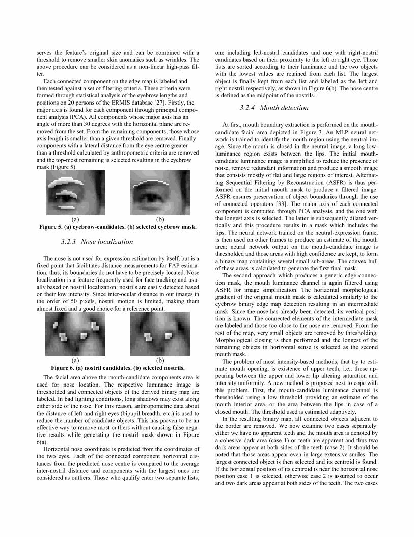
mask (Figure 5).
(a)
(b)
Figure 5. (a) eyebrow-candidates. (b) selected eyebrow mask.
3.2.3 Nose localization
The nose is not used for expression estimation by itself, but is a
fixed point that facilitates distance measurements for FAP estima-
tion, thus, its boundaries do not have to be precisely located. Nose
localization is a feature frequently used for face tracking and usu-
ally based on nostril localization; nostrils are easily detected based
on their low intensity. Since inter-ocular distance in our images in
the order of 50 pixels, nostril motion is limited, making them
almost fixed and a good choice for a reference point.
(a)
(b)
Figure 6. (a) nostril candidates. (b) selected nostrils.
The facial area above the mouth-candidate components area is
used for nose location. The respective luminance image is
thresholded and connected objects of the derived binary map are
labeled. In bad lighting conditions, long shadows may exist along
either side of the nose. For this reason, anthropometric data about
the distance of left and right eyes (bipupil breadth, etc.) is used to
reduce the number of candidate objects. This has proven to be an
effective way to remove most outliers without causing false nega-
tive results while generating the nostril mask shown in Figure
6(a).
Horizontal nose coordinate is predicted from the coordinates of
the two eyes. Each of the connected component horizontal dis-
tances from the predicted nose centre is compared to the average
inter-nostril distance and components with the largest ones are
considered as outliers. Those who qualify enter two separate lists,
one including left-nostril candidates and one with right-nostril
candidates based on their proximity to the left or right eye. Those
lists are sorted according to their luminance and the two objects
with the lowest values are retained from each list. The largest
object is finally kept from each list and labeled as the left and
right nostril respectively, as shown in Figure 6(b). The nose centre
is defined as the midpoint of the nostrils.
3.2.4 Mouth detection
At first, mouth boundary extraction is performed on the mouth-
candidate facial area depicted in Figure 3. An MLP neural net-
work is trained to identify the mouth region using the neutral im-
age. Since the mouth is closed in the neutral image, a long low-
luminance region exists between the lips. The initial mouth-
candidate luminance image is simplified to reduce the presence of
noise, remove redundant information and produce a smooth image
that consists mostly of flat and large regions of interest. Alternat-
ing Sequential Filtering by Reconstruction (ASFR) is thus per-
formed on the initial mouth mask to produce a filtered image.
ASFR ensures preservation of object boundaries through the use
of connected operators [33]. The major axis of each connected
component is computed through PCA analysis, and the one with
the longest axis is selected. The latter is subsequently dilated ver-
tically and this procedure results in a mask which includes the
lips. The neural network trained on the neutral-expression frame,
is then used on other frames to produce an estimate of the mouth
area: neural network output on the mouth-candidate image is
thresholded and those areas with high confidence are kept, to form
a binary map containing several small sub-areas. The convex hull
of these areas is calculated to generate the first final mask.
The second approach which produces a generic edge connec-
tion mask, the mouth luminance channel is again filtered using
ASFR for image simplification. The horizontal morphological
gradient of the original mouth mask is calculated similarly to the
eyebrow binary edge map detection resulting in an intermediate
mask. Since the nose has already been detected, its vertical posi-
tion is known. The connected elements of the intermediate mask
are labeled and those too close to the nose are removed. From the
rest of the map, very small objects are removed by thresholding.
Morphological closing is then performed and the longest of the
remaining objects in horizontal sense is selected as the second
mouth mask.
The problem of most intensity-based methods, that try to esti-
mate mouth opening, is existence of upper teeth, i.e., those ap-
pearing between the upper and lower lip altering saturation and
intensity uniformity. A new method is proposed next to cope with
this problem. First, the mouth-candidate luminance channel is
thresholded using a low threshold providing an estimate of the
mouth interior area, or the area between the lips in case of a
closed mouth. The threshold used is estimated adaptively.
In the resulting binary map, all connected objects adjacent to
the border are removed. We now examine two cases separately:
either we have no apparent teeth and the mouth area is denoted by
a cohesive dark area (case 1) or teeth are apparent and thus two
dark areas appear at both sides of the teeth (case 2). It should be
noted that those areas appear even in large extensive smiles. The
largest connected object is then selected and its centroid is found.
If the horizontal position of its centroid is near the horizontal nose
position case 1 is selected, otherwise case 2 is assumed to occur
and two dark areas appear at both sides of the teeth. The two cases

are quite distinguishable through this process. In case 2, the se-
cond largest connected object is also selected. A new binary map
is created containing either one object in case 1 or both objects in
case 2; the convex hull of this map is then calculated.
The detected lip corners provide a robust estimation of mouth
horizontal extent but are not adequate to detect mouth opening.
Therefore, the latter binary mask is expanded to include the lower
lips. An edge map is created as follows: the mouth image gradient
is calculated in the horizontal direction, and is thresholded by the
median of its positive values. This mask contains objects close to
the lower middle part of the mouth, which are sometimes missed
because of the lower teeth. The two masks have to be combined to
a final mask. An effective way of achieving this is to keep from
both masks objects which are close to each other.
3.3 Final Masks Generation and Confi-
dence Estimation
Each facial feature’s masks must be fused together to produce a
final mask for that feature. The most common problems, especial-
ly encountered in low quality input images, include connection
with other feature boundaries or mask dislocation due to noise. In
some cases some masks may have completely missed their goal
and provide a completely invalid result. Outliers such as illumina-
tion changes and compression artifacts cannot be predicted and so
individual masks have to be re-evaluated and combined on each
new frame.
The proposed algorithms presented in section 3.2 produce a
mask for each eyebrow, nose coordinates, four intermediate mask
estimates for each eye and three intermediate mouth mask esti-
mates. The four masks for each eye and three mouth masks must
be fused to produce a final mask for each feature. Since validation
can only be done on the end result of each intermediate mask, we
unfortunately cannot give different parts of each intermediate
mask different confidence values, so each pixel of those masks
will share the same value. We propose validation through testing
against a set of anthropometric conformity criteria. Since, howev-
er some of these criteria relate either to aesthetics or to transient
feature properties, we cannot apply strict anthropometric judg-
ment.
For each mask of every feature, we employ a set of validation
measurements, which are then combined to a final validation tag
for that mask. Each measurement produces a validation estimate
value depending on how close it is to the usually expected feature
shape and position, in the neutral expression. Expected values for
these measurements are defined from anthropometry data [29] and
from images extracted from video sequences of 20 persons in our
database [27]. Thus, a validation tag between [0,1] is attached to
each mask, with higher values denoting proximity to the most
expected measurement values. We want masks with very low
validation tags to be discarded from the fusion process and thus
those are also prevented from contribution on final validation
tags.
3.4 From FP to FAP Estimation
A 25-dimensional distance vector is created containing vertical
and horizontal distances between 19 extracted FPs, as shown in
Figure 7. Distances are normalized using scale-invariant MPEG-4
units, i.e. ENS, MNS, MW, IRISD and ES [25]. Unit bases are
measured directly from FP distances on the neutral image; for
example ES is calculated as |FP9,FP13|.
3
4
11
14
15
20 21
1
57
9
12
16
18
24
2
6 8
10
13
17
19
24
22
22
1
10
2 3
16
8
97
12
11
6 5
4
14
13
17
15
18
19
12
8
FP #
Distance #
Figure 7. Feature Point Distances
The distance vector is created once for the neutral-expression
image and for each of the subsequent frames FAPs are calculated
by comparing them with the neutral frame. The value of each FAP
is calculated from a set of geometric rules based on variations of
distances from immovable points on the face. For example, the
inner eyebrow FAPs are calculated by projecting vertically the
distance of the inner eye corners, points 8 and 12 in Figure 7, to
points 3 and 6 and comparing it to their distance in the neutral
frame. A more detailed discussion on this procedure is found at
[34].
4. ACOUSTIC FEATURES EXTRACTION The features used in this work are exclusively based on prosody
and related to pitch and rhythm. All information related to emo-
tion that one can extract from pitch is probably not only in these
features, but the motivation of this approach is in the desire to
develop and use a high level of speech prosody analysis, calculate
as many features as possible and then reduce them to those uncor-
related with each other and relevant to expressivity ([42], [44]).
We analyzed each tune with a method employing prosodic repre-
sentation based on perception called ‘Prosogram’ [11]. Prosogram
is based on a stylization of the fundamental frequency data (con-
tour) for vocalic (or syllabic) nuclei. It gives globally for each
voiced nucleus a pitch and a length. According to a 'glissando
treshold' in some cases we don’t get a fixed pitch but one or more
lines to define the evolution of pitch for this nucleus. This repre-
sentation is in a way similar to the 'piano roll' representation used
in music sequencers. This method, based on the Praat environ-
ment, offers the possibility of automatic segmentation based both
on voiced part and energy maxima. From this model - representa-
tion stylization we extracted several types of features: pitch inter-
val based features, nucleus length features and distances between
nuclei.
In musical theory, ordered pitch interval is the distance in semi-
tones between two pitches upwards or downwards. For instance,
the interval from C to G upward is 7, but the interval from G to C
downwards is −7. Using integer notation (and eventually modulo
12) ordered pitch interval, ip, may be defined, for any two pitches
x and y, as:
,
,
ip y x x y
ip x y y x
(1)

In this study we considered pitch intervals between successive
voiced nuclei. For any two pitches x and y, where x precedes y, we
calculate the interval ,ip x y y x , then deduce the follow-
ing features.
For each tune, feature (f1) is the minimum of all the successive
intervals in the tune. In a similar way, we extract the maximum
(f2), the range (absolute difference between minimum and maxi-
mum) (f3), of all the successive intervals in each tune. Using the
same measure, we also deduce the number of positive intervals
(f4) and the number of negative intervals (f5). Using the absolute
value, a measure equivalent to the unordered pitch interval in
music theory, we deduce a series of similar features: minimum
(f6), maximum (f7), mean (f8) and range (f9) of the pitch interval.
Another series of features is also deduced from the ratio between
successive intervals, here again maximum (f10), minimum (f11),
mean (f12) and range (f13) of these ratios give the related fea-
tures. In addition to the aforementioned features, the usual pitch
features have also been used such as fundamental frequency min-
imum (f14), maximum (f15), mean (f16) and range (f17). The
global slope of the pitch curve (f18), using linear regression, has
also been added.
As was previously said, each segment (voiced “nucleus” if it is
voiced) of this representation has a length, and this has also been
used in each tune to extract features related to rhythm. These fea-
tures are, as previously, maximum (f19), minimum (f20), mean
(f21) and range (f22). Distances between segments have also been
used as features and the four last features we used are maximum
(f23), minimum (f24), mean (f25) and range (f26) of these dis-
tances.
5. EXPERIMENTAL RESULTS
5.1 Fusion of visual and acoustic features
In the area of unimodal emotion recognition there have been many
studies using different, but single, modalities. Facial expressions
[12], [13], [18], vocal features [14], [15] and physiological sig-
nals [16] have been used as inputs during these attempts, while
multimodal emotion recognition is currently gaining ground ([19],
[20], [43], [47]).
As primary material we consider the audiovisual content collected
using the SAL approach. This material was labeled using
FeelTrace [23] by four labelers. The activation-valence coordi-
nates from the four labelers were initially clustered into quadrants
and were then statistically processed so that a majority decision
could be obtained about the unique emotion describing the given
moment. The corpus under investigation was segmented into 1000
tunes of varying length. For every tune the input vector, as far as
facial features is concerned, consisted of the FAPs produced by
the processing of the frames of the tune. The acoustic input vector
consisted of only one value per SBPF (Segment Based Prosodic
Feature) per tune. The fusion was performed on a frame basis,
meaning that the values of the SBPFs were repeated for every
frame of the tune. This approach was preferred because it pre-
served the maximum of the available information since SBPFs are
only meaningful for a certain time period and cannot be calculated
per frame.
5.2 Recurrent Neural Networks
A wide variety of machine learning techniques have been used in
emotion recognition approaches ([13], [18], [42]). Especially in
the multimodal case [41], they all employ a large number of au-
dio, visual or physiological features, a fact which usually impedes
the training process; therefore, we need to find a way to reduce
the number of utilized features by picking out only those related
to emotion. An obvious choice for this is neural networks, since
they enable us to pinpoint the most relevant features with respect
to the output, usually by observing their weights. Although such
architectures have been successfully used to solve problems that
require the computation of a static function, where output depends
only upon the current input, and not on any previous inputs, this
is not the case in the domain of emotion recognition. One of the
reasons for this is that expressivity is a dynamic, time-varying
concept, where it is not always possible to deduce an emotional
state merely by looking at a still image. As a result, Bayesian ap-
proaches which lend themselves nicely to similar problems [22],
need to be extended to include support for time-varying features.
Picard 7 proposes the use of Hidden Markov Models (HMMs) to
model discrete emotional states (interest, joy or distress) and use
them to predict the probability of each one, given a video of a
user. However, this process needs to build a single HMM for each
of the examined cases (e.g. each of the universal emotions), mak-
ing it more suitable in cases where discrete emotions need to be
estimated. In our case, building dedicated HMMs for each of the
quadrants of the emotion representation would not suffice, since
each of them contains emotions expressed with highly varying
features (e.g. anger and fear in the negative/active quadrant).
A more suitable choice would be RNNs (Recurrent Neural Net-
works) where past inputs influence the processing of future inputs
[38]. RNNs possess the nice feature of modelling explicitly time
and memory ([39], [40], [46]), catering for the fact that emotional
states are not fluctuating strongly, given a short period of time.
Additionally, they can model emotional transitions and not only
static emotional representations, providing a solution for diverse
feature variation and not merely for neutral to expressive and back
to neutral, as would be the case for HMMs.
The implementation of a RNN we used was based on an Elman
network [10], [38]. The input vectors were formed as described
earlier and the output classes were 4 (3 for the possible emotion
quadrants, since the data for the positive/passive quadrant was
negligible, and one for neutral affective state) resulting in a da-
taset consisting of around 10000 records. The training/testing
dataset was on a 3 to 1 ratio. The classification efficiency, for
facial only and audio only, was measured at 67% and 73% respec-
tively but combining the two modalities we achieved a recogni-
tion rate of 79%. This fact illustrates the ability of the proposed
method to take advantage of multimodal information and the re-
lated analysis.
6. CONCLUSIONS – FUTURE WORK
Naturalistic data goes beyond extreme emotions and concentrates
on more natural emotional episodes that happen more frequently
in everyday discourse. In this paper, we described a feature-based
approach that tackles most of the intricacies of every-day audio-
visual HCI and models the time-varying nature of these features in
cases of expressivity. Most approaches focus on the detected of
(mainly) visual features in pre-recorded, acted datasets and the
utilization of machine learning algorithms to estimate the illustrat-
ed emotions. Even in cases of multimodality, features are fed into
the machine learning algorithms without any real attempt to find
structure and correlations between the features themselves and the
estimated result. Neural networks are a nice solution to finding
such relations, thus coming up with comprehensible connections
between the input (features) and the output (emotion).
The fact that we use naturalistic and not acted data introduces a
number of interesting issues, for example segmentation of the
discourse in tunes. During the experiment, tunes containing a
small number of frames (less than 5 frames, i.e. 0.2 seconds) were
found to be error prone and classified close to chance level (not
better than 37%). This is attributed to the fact that emotion in the
speech channel needs at least half a second to be expressed via
wording, as well as to the internal structure of the Elman network
which works better with a short-term memory of ten frames. From
a labeling point of view, ratings from four labelers are available;
in some cases, experts would disagree in more than 40% of the
frames in a single tune. In order to integrate this fact, the decision
system has to take into account the interlabeller disagreement, by
comparing this to the level of disagreement with the automatic
estimation. One way to achieve this, is the modification of the
Williams Index, which is used to this effect for the visual channel
in [13].
A future direction regarding the features themselves is to model
the correlation between phonemes and FAPs. In general, FPs from
the mouth area do not contribute much when the subject is speak-
ing; however, consistent phoneme detection could help differenti-
ate expression-related deformation (e.g. a smile) to speech-related.
Regarding the speech channel, the multitude of the currently de-
tected features is hampering the training algorithms. To overcome
this, we need to evaluate the importance/prominence of features
so as to conclude on the influence they have on emotional transi-
tion. This can be achieved through statistical analysis (PCA analy-
sis, K-Means Cluster Analysis, Two Step Cluster Analysis, Hier-
archical Cluster Analysis) or Sensitivity Analysis [24].
7. ACKNOWLEDGMENTS Current work was funded by the 03ED375 research project, im-
plemented within the framework of the ''Reinforcement Pro-
gramme of Human Research Manpower'' (PENED) and co-
financed by National and Community Funds (25% from the Greek
Ministry of Development-General Secretariat of Research and
Technology and 75% from E.U.-European Social Fund).
8. REFERENCES [1] R. W. Picard, Affective Computing, MIT Press, 1997.
[2] A. Jaimes, Human-Centered Multimedia: Culture, Deploy-
ment, and Access, IEEE Multimedia Magazine, Vol. 13,
No.1, 2006.
[3] A. Pentland, A., Socially Aware Computation and Commu-
nication, Computer, vol. 38, no. 3, pp. 33-40, 2005.
[4] R. W. Picard, Towards computers that recognize and respond
to user emotion, IBM Syst. Journal, 39 (3–4), 705–719,
2000.
[5] A. Mehrabian, Communication without Words, Psychology
Today, vol. 2, no. 4, pp. 53-56, 1968.
[6] A.J. Fridlund, Human Facial Expression: An Evolutionary
Perspective, Academic Press, 1994.
[7] M, Pantic, Face for Interface, in The Encyclopedia of Multi-
media Technology and Networking, M. Pagani, Ed., Idea
Group Reference, vol. 1, pp. 308-314, 2005.
[8] A. Nogueiras, A. Moreno, A. Bonafonte and J.B. Mariño,
Speech emotion recognition using hidden markov models.
Proceedings of Eurospeech, Aalborg, Denmark, 2001.
[9] J. Lien, Automatic recognition of facial expressions using
hidden markov models and estimation of expression intensi-
ty, Ph.D. dissertation, Carnegie Mellon University, Pittsburg,
PA, 1998.
[10] J.L. Elman, Finding structure in time, Cognitive Science, vol.
14, 1990, pp. 179-211.
[11] P. Mertens, The Prosogram: Semi-Automatic Transcription
of Prosody based on a Tonal Perception Model. in B. Bel &
I. Marlien (eds.), Proc. of Speech Prosody, Japan, 2004.
[12] K. Karpouzis, A. Raouzaiou, A. Drosopoulos, S. Ioannou, T.
Balomenos, N. Tsapatsoulis and S. Kollias, Facial expression
and gesture analysis for emotionally-rich man-machine inter-
action, in N. Sarris, M. Strintzis, (eds.), 3D Modeling and
Animation: Synthesis and Analysis Techniques, pp. 175-200,
Idea Group Publ., 2004.
[13] S. Ioannou, A. Raouzaiou, V. Tzouvaras, T. Mailis, K.
Karpouzis, S. Kollias, Emotion recognition through facial
expression analysis based on a neurofuzzy network, Neural
Networks, Elsevier, Vol. 18, Issue 4, May 2005, pp. 423-435
[14] R. Cowie and E. Douglas-Cowie, Automatic statistical analy-
sis of the signal and prosodic signs of emotion in speech. In
Proc. International Conf. on Spoken Language Processing,
pp. 1989–1992, 1996.
[15] K.R. Scherer, Adding the affective dimension: A new look in
speech analysis and synthesis, In Proc. International Conf.
on Spoken Language Processing, pp. 1808–1811, 1996.
[16] R.W. Picard, E. Vyzas, and J. Healey, Toward machine emo-
tional intelligence: Analysis of affective physiological state,
IEEE Trans. on Pattern Analysis and Machine Intelligence,
23(10):1175–1191, 2001.
[17] L.S. Chen, Joint processing of audio-visual information for
the recognition of emotional expressions in human-computer
interaction, PhD thesis, University of Illinois at Urbana-
Champaign, Dept. of Electrical Engineering, 2000.
[18] M. Pantic and L.J.M. Rothkrantz, Automatic analysis of
facial expressions: The state of the art. IEEE Trans. on Pat-
tern Analysis and Machine Intelligence, 22(12):1424–1445,
2000.
[19] L.C. De Silva and P.C Ng, Bimodal emotion recognition, In
Proc. Automatic Face and Gesture Recognition, pp. 332–
335, 2000.
[20] L.S. Chen and T.S. Huang, Emotional expressions in audio-
visual human computer interaction, In Proc. International
Conference on Multimedia and Expo, pp. 423–426, 2000.
[21] L.M. Wang, X.H. Shi, G.J. Chen, H.W. Ge, H.P. Lee, Y .C.
Liang, Applications of PSO Algorithm and OIF Elman Neu-

ral Network to Assessment and Forecasting for Atmospheric
Quality, ICANNGA 2005, 2005
[22] N. Sebe, I. Cohen, T.S. Huang, Handbook of Pattern Recog-
nition and Computer Vision, World Scientific, January 2005
[23] R. Cowie, E. Douglas-Cowie, S. Savvidou, E. McMahon, M.
Sawey and M. Schröder, FEELTRACE: An instrument for
recording perceived emotion in real time, ISCA Workshop on
Speech and Emotion, Northern Ireland, pp. 19-24, 2000.
[24] AP Engelbrecht, I. Cloete, A Sensitivity Analysis Algorithm
for Pruning Feedforward Neural Networks, IEEE Interna-
tional Conference in Neural Networks, Washington, Vol 2,
1996, pp 1274-1277.
[25] A. Murat Tekalp, Joern Ostermann, Face and 2-D mesh ani-
mation in MPEG-4, Signal Processing: Image Communica-
tion 15, Elsevier, pp. 387-421, 2000.
[26] Rein-Lien Hsu, Mohamed Abdel-Mottaleb, Anil K. Jain,
Face Detection in Color Images, IEEE Transactions on Pat-
tern Analysis and Machine Intelligence, Vol.24, No.5, May
2002
[27] ERMIS, Emotionally Rich Man-machine Intelligent System
IST-2000-29319, http://www.image.ntua.gr/ermis
[28] HUMAINE IST, Human-Machine Interaction Network on
Emotion, 2004-2007, http://www.emotion-research.net
[29] J. W. Young, Head and Face Anthropometry of Adult U.S.
Civilians, FAA Civil Aeromedical Institute, 1963-1993 (final
report 1993)
[30] R. Fransens, Jan De Prins, SVM-based Nonparametric Dis-
criminant Analysis, An Application to Face Detection, Ninth
IEEE International Conference on Computer Vision, Vol-
ume 2, October 13 - 16, 2003.
[31] Kin-Man Lam and Hong Yan, Locating And Extracting the
Eye in Human Face Images, Pattern Recognition, Vol.29,
No.5, 1996, pp. 771-779.
[32] C. Tomasi and T. Kanade, Detection and Tracking of Point
Features, Carnegie Mellon University Technical Report
CMU-CS-91-132, April 1991.
[33] L. Vincent, Morphological Grayscale Reconstruction in Im-
age Analysis: Applications and Efficient Algorithms, IEEE
Trans. Image Processing, vol. 2, no. 2, 1993, pp. 176-201.
[34] A. Raouzaiou, N. Tsapatsoulis, K. Karpouzis and S. Kollias,
Parameterized facial expression synthesis based on MPEG-4,
EURASIP Journal on Applied Signal Processing, Vol. 2002,
No 10, 2002, pp. 1021-1038.
[35] M. H. Yang, D. Kriegman, N. Ahuja, Detecting Faces in
Images: A Survey, IEEE Trans. on Pattern Analysis and Ma-
chine Intelligence, Vol.24(1), 2002, pp. 34-58.
[36] P. Ekman and W. Friesen, Pictures of Facial Affect, Palo
Alto, CA: Consulting Psychologists Press, 1978.
[37] U. Williams, K. N. Stevens, Emotions and Speech: some
acoustical correlates, JASA 52, pp. 1238-1250, 1972.
[38] Mathworks, Manual of Neural Network Toolbox for
MATLAB
[39] S. Haykin. Neural Networks: A Comprehensive Foundation.
Macmillan, New York, 1994.
[40] H. G. Zimmermann, R. Grothmann, A. M. Schaefer, and Ch.
Tietz. Identification and forecasting of large dynamical sys-
tems by dynamical consistent neural networks. In S. Haykin,
T. Sejnowski J. Principe, and J. McWhirter, editors, New Di-
rections in Statistical Signal Processing: From Systems to
Brain. MIT Press, 2006.
[41] M. Pantic, N. Sebe, J. Cohn, T. Huang, Affective Multimodal
Human-Computer Interaction, Proceedings of the 13th an-
nual ACM international conference on Multimedia, pp. 669
– 676, 2005.
[42] R. Cowie, E. Douglas-Cowie, N.Tsapatsouulis, G. Votsis, S.
Kollias, W. Fellenz and J. G. Taylor, Emotion Recognition in
Human-Computer Interaction, IEEE Signal Processign
Magazine, pp 33- 80, January 2001.
[43] M. Pantic and L.J.M. Rothkrantz, Towards an Affect-
sensitive Multimodal Human-Computer Interaction, Pro-
ceedings of the IEEE, vol. 91, no. 9, pp. 1370-1390, 2003.
[44] P. Oudeyer, The production and recognition of emotions in
speech: features and algorithms. International Journal of
Human Computer Interaction, 59(1-2):157-183, 2003.
[45] I. Cohen, A. Garg, and T. S. Huang, Emotion Recognition
using Multilevel-HMM, NIPS Workshop on Affective Com-
puting, Colorado, Dec 2000.
[46] F. Freitag, E. Monte, Acoustic-phonetic decoding based on
Elman predictive neural networks, Proceedings of ICSLP 96,
Fourth International Conference on, Page(s): 522-525, vol.1.
[47] Z. Zeng, J. Tu, M. Liu, T.S. Huang, Multi-stream Confidence
Analysis for Audio-Visual Affect Recognition, ACII 2005,
pp. 964-971.
Top Related