


Languages
Pages
Legal


General rights Copyright and moral rights for the publications made accessible in the public portal are retained by the authors and/or other copyright owners and it is a condition of accessing publications that users recognise and abide by the legal requirements associated with these rights.
Users may download and print one copy of any publication from the public portal for the purpose of private study or research.
You may not further distribute the material or use it for any profit-making activity or commercial gain
You may freely distribute the URL identifying the publication in the public portal If you believe that this document breaches copyright please contact us providing details, and we will remove access to the work immediately and investigate your claim.
Downloaded from orbit.dtu.dk on: May 13, 2020
Migration of plasticisers from PVC and other polymers
Lundsgaard, Rasmus
Publication date:2011
Document VersionPublisher's PDF, also known as Version of record
Link back to DTU Orbit
Citation (APA):Lundsgaard, R. (2011). Migration of plasticisers from PVC and other polymers. Technical University of Denmark.

Migration of
plasticisers from PVC
and other polymers
Understanding of additive
migration and diffusion in
Polyvinyl chloride (PVC) and Polyolefins
Rasmus Lundsgaard
October 15, 2010
Migration of plasticisers from
PVC and other polymersProject period: 1/7-2007 - 30/9-2010
PhD thesis
Supervisors: Georgios M. Kontogeorgis (CERE, DTU Chemical Engineering),
Bjarne Nielsen (DANISCO A/S)
& Ulrik Aunskjær (DANISCO A/S)
Center for Energy Ressources Engineering (CERE)
Department of Chemical and Biochemical Engineering
Technical University of Denmark
Rasmus Lundsgaard


Preface
This thesis is submitted in partial fulfillment of the requirements to obtain the Doctor of Phi-
losophy degree at the Technical University of Denmark (DTU). The work has been carried out
at the CERE-DTU (Center for Energy Ressources Engineering, formerly known as IVC-SEP)
at the Department of Chemical and Biochemical Engineering, DTU, under the supervision of
Professors Georgios M. Kontogeorgis from CERE-DTU and Bjarne Nielsen and Ulrik Aunskjær,
both from Danisco A/S.
The project was financially supported by 1/3 form the Technical University of Denmark, 1/3
from the Graduate School in Chemical Engineering and finally 1/3 by Danisco A/S. The author
gratefully acknowledges their support.
I would like to express my deepest gratitude to my main supervisor Prof. Georgios M. Konto-
georgis for his endless support and encouragement over the last four years since he accepted to
be my supervisor on my master project. He is truly my scientific adviser and mentor, and has
always shown support and genuine interest in my project. Also I am deeply grateful to Prof.
Georgios M. Kontogeorgis for introducing me to the vast network of great Greek scientists in
the international community.
One of these is Prof. Ioannis G. Economou of the National Center for Scientific Research
”Demokritos” in Athena, Greece, who soon also became an important adviser to me. I am
deeply grateful to him for always finding time to discuss and advise me in the problems I en-
countered during my work on molecular simulations. Moreover I would very much like to thank
him and his co-workers (Niki, Zoe, George and Eleni) at N.C.S.R. Demokritos to find space and
time to have me visiting the research center in Athens. My two long visits at the research center
in Athens have given me an opportunity to learn the greek way of living, and Athens will for
always be my second home.
I would also like to thank Nuno Garrido from the Chemical Engineering Department at Uni-
versity of Porto, Portugal, for our sharing of knowledge and code for molecular simulation with
the GROMACS software, and Søren Enemark from Department of Chemical and Biomolecular
Engineering at the National University of Singapore sharing of code and testing of the developed
hydrogen bond cluster counting code.
I would also like to express my gratitude to Danisco A/S and especially Bjarne Nielsen, Ulrik
– i –

Aunskjær, Torkil F. Jensen and Jørgen K. Kristiansen for finding time for me in their always
busy schedule at Danisco. It was really a valuable experience to me to become a full member
of the development team at Danisco on the new antistatic additive project, and through this
project learn how my knowledge through the PhD project directly could get to use.
I am also deeply honored that Dr. Otto G. Piringer has taken time to discuss with me on the
migration of plasticisers in highly plasticised PVC, and moreover that he has shown personal
interest in this project and its progress.
To the colleagues at KT and especially in the CERE group I would like to express my gratitude
to the many joyful moments I have shared with you over the last four years. I would especially
like to thank Ane S. Avlund for our many discussions on our projects and of course for her
company during our professional trips together. Also I am deeply grateful to the guidance and
help by Philip L. Fosbøl on Matlab programming, and our many discussions on understanding
of the acetic acid data and the development of the antistatic additive migration model.
Lastly I would like to thank my family and friends for nodding and smiling understandingly
when I explained you in many details on the complex problems in this project I was trying
to solve, and for moments together with reminding me that there are other things in life than
molecular dynamics and migration modeling.
Rasmus Lundsgaard
Søborg, Denmark
October 15, 2010
– ii –

I would like to devote this thesis to my father, who has always encouragedme to be curious and question the world around me. You were alwayswilling to answer my numerous questions, and always in the most truthfulway...
– iii –

Summary
The main purpose of this thesis is to investigate, from a modeling point of view, the migra-
tion of GRINDSTEDr SOFT-N-SAFE (SNS) and other plasticisers from polyvinyl chloride
(PVC) and polyolefin food package materials and into foodstuff (specifically the four food
simulants set by EU legislation). In this work it is shown how diffusion coefficients can
be obtained by regression of experimental migration data plotted as the square root of
time. This was done from plasticiser migration data of GRINDSTEDr SOFT-N-SAFE,
GRINDSTEDr ACETEM 95 CO (Acetem) and Epoxidised Soybean Oil (ESBO) migrating
from Polyvinyl Chloride (PVC) and into iso-octane at 20◦C, 40◦C and 60◦C. Using these
experimentally obtained diffusion coefficients the migration was modeled using two analyti-
cal models with relatively good accuracy. The diffusion coefficient in highly plasticised PVC
should, however, not be considered uniform over the whole polymer layer when the migrant
is the plasticiser itself.
It was attempted to predict the diffusion coefficient of SNS in highly plasticised PVC from
pure component data alone, using the model by Vrentas and Vrentas, which is based on
the free volume theory. The results, however, showed that the model under-predicts the
experimental diffusion coefficient values. These experimentally obtained values should be
regarded as average diffusion coefficient values of the whole polymer and lower than the
diffusion coefficient of the fully plasticised PVC. Instead of using this elaborated complex
model, it was decided to use the much simpler semi-empirical model by Piringer. Using this
simple model, with a polymer-specific parameter obtained from ESBO migration data alone,
it was possible to estimate diffusion coefficients for Acetem and SNS. The results were close
to the experimentally obtained diffusion coefficients at 20◦C, except at higher temperatures.
Using the finite element mesh method in Matlab and COMSOL environments the migration
was modeled with a diffusion coefficient able to change with local plasticiser concentra-
tion. Three different models for this plasticiser concentration dependence of the diffusion
coefficient were evaluated. All models performed similarly, with better predicting ability
compared to modeling with a static diffusion coefficient.
This numerical solution by the finite element mesh method has also been used to model
the migration of an antistatic additive to the surface of Low Density Polyethylene (LDPE)
and Poly Propylene (PP). It was possible with a newly developed model to estimate the
migration with very high accuracy. This result leads to the somewhat surprising conclusion
that the controlling step in the migration of the additive to the surface was not the migration
within the polymer bulk. Migration is probably due to a temperature dependent partitioning
of the additive between the polymer bulk and the surface layer.
The possibility of using molecular dynamics calculations to estimate the partition coefficients
of additives between polymers and foodstuff was also investigated. The development of the
methodology was done against experimental data of a system composed of a hydrophilic or a
hydrophobic additive between LDPE and different ethanol/water mixtures. The calculated
partition coefficients of different additives between LDPE and ethanol/water were correlated
with high accuracy against experimental data. To extend the methodology to acetic acid
– iv –

systems (food simulant B), it was chosen firstly to investigate the predictive capabilities of
the TraPPE, OPLS-AA and CHARMM27 force fields for pure acetic acid and acetic acid /
water mixtures. None of the three force fields was able to predict satisfactorily the density
of acetic acid / water mixtures. Only the CHARMM27 force field was able to predict the
local density maxima of the system.
A hydrogen bond connectivity counting code was developed for investigating the clustering of
acetic acid. Statistics using the cluster counting code showed that the acetic acid molecules in
the liquid phase mostly formed chain-like structures, with chains of 2 and 3 molecules in size
to be the most predominant ones. Furthermore, the ability of the force fields to predict the
enthalpy of vaporization was tested. All three force fields over-predict this property, resulting
to a value about twice the experimental one (≈ 50kJ/mol compared to 23.7kJ/mol). The gas
phase consisted almost entirely of monomers, where experimental Pressure-Volume data of
the gas phase at 298K and 1 bar give a dimer fraction of around 80-90%. This dimer fraction
in the gas phase was elevated using higher atomic charges as shown by Chocholousova et al.[J.
Chocholousova, J. Vacek, and P. Hobza; J. Phys. Chem. A; 107, 17, (2003), 3086-3092],
but the calculated enthalpy of vaporization was still almost twice as high. It was shown that
most literature data listing a value of ≈ 50kJ/mol originate from the work by Konicek and
Wadso[J. Konicek and I. Wadso; Acta Chem. Scand.; 24, 7, (1970), 2612-2616] from 1970.
In the same work is explained how the enthalpy of vaporization of acetic acid theoretically
can be seen as consisting of two contributions, the ”pure” enthalpy of vaporization of the
monomer and the enthalpy of dissociation. It is important that this theoretically-derived
”pure”enthalpy of vaporization (which is ≈ 50kJ/mol) is not confused with the experimentally
obtained enthalpy of vaporization (23.7kJ/mol). The OPLS-AA force field is parameterized
towards the theoretical ”pure” enthalpy of vaporization in a correct way, by only calculating
the energy difference for the single acetic acid monomer molecule between the two phases.
However simulations in this work have shown that these parameters do not allow the force
field to predict the gas phase dimer fraction accurately.
Overall from this work it can be concluded that a full prediction of migration in polyolefins
can be obtained using the numerical solution by finite element mesh together with diffusion
coefficients obtained from the Piringer model and partition coefficient by molecular dynam-
ics. For the complex system of migration of plasticisers in highly plasticised PVC, a full
predicitive model was not obtained. A model was, however, developed for this system that
predicts satisfactorily with only 1 or 2 adjustable parameters to plasticiser migration from
PVC.
– v –

Resume
(Summary in Danish)
Hovedformalet med denne afhandling er at undersøge, fra et modelleringssynspunkt, migra-
tionen af GRINDSTEDr SOFT-N-SAFE (SNS) og andre blødgørere fra fødevareemballager
af polyvinylchlorid (PVC) og polyolefiner og ind i fødevarer (specielt de fire fødevaresim-
ulanter fastsat i EU’s lovgivning). I dette arbejde er det vist, hvordan diffusionskoeffi-
cienter kan fas ved regression af eksperimentelle migration data plottet som funktion af
kvadratroden af tid. Dette blev gjort i dette arbejde med data fra migrationen af blødgør-
erne SNS GRINDSTEDr ACETEM 95 CO (Acetem) og Epoxideret sojaolie (ESBO) fra
polyvinylchlorid (PVC) og ud i iso-oktan ved 20◦C, 40◦C og 60◦C. Ved hjælp af disse eksper-
imentelt opnaede diffusionskoefficienter, blev migrationen modelleret ved hjælp af to ana-
lytiske modeller med relativt god nøjagtighed. Diffusionskoefficienten i blødgjort PVC bør
dog ikke betragtes som ensartet over hele polymeren hvis migrationen netop er af blødgøreren
selv.
Det blev forsøgt at estimere diffusionskoefficienten af SNS i blødgjort PVC fra ren kompo-
nent data alene, udfra modellen af Vrentas og Vrentas, som er baseret pa den frie volume
teori. Resultaterne viste imidlertid, at modellen underestimerer de eksperimentelle diffu-
sionskoefficientværdier. Disse beregnede diffusionskoefficienter fra eksperimentelle data, bør
betragtes som en gennemsnitsdiffusionskoefficient for hele polymeren og dermed lavere end
diffusionskoefficienten i den fuldt blødgjorte PVC. I stedet for at bruge denne komplekse
model, blev det besluttet at anvende den enklere semi-empiriske model af Piringer. Ved at
bruge denne simple model, med en polymer-specifik parameter kun fra ESBO data, var det
muligt at estimere diffusionskoefficienter for Acetem og SNS. Resultaterne var tæt pa de
eksperimentelt opnaede diffusionskoefficienter ved 20◦C, men ikke ved højere temperaturer.
Ved brug af finite element mesh metoden i Matlab og COMSOL, blev migrationen modelleret
med en koncentrationsafhængig diffusionskoefficient, der ændrer sig med den lokale blødgører
koncentration. Tre forskellige modeller for denne blødgører koncentrationsafhængighed af
diffusionskoefficenten blev evalueret. Alle modeller var ca. lige succesfulde, med generelt
bedre resultater end modellering med en statisk diffusionskoefficient.
Den numeriske løsning med finite element mesh metoden er ogsa blevet brugt til at mod-
ellere et antistatisk additivs migration til overfladen af Low Density Polyethylen (LDPE) og
Poly Propylen (PP). Det var muligt med en nyudviklet model at estimere migration med
meget stor nøjagtighed. Dette resultat førte til den lidt overraskende konklusion, at det kon-
trollerende led i migrationen af additivet til overfladen ikke var migration i selve polymeren.
Migration er sandsynligvis kontrolleret af en temperatur afhængig partitionskoefficient for
additivet imellem polymer og overfladelaget.
Muligheden for at anvende molekyle simuleringer ved ”Molecular dynamics” beregninger til
estimering af partitionskoefficienter for additiver i de forskellige polymerer og fødevarer blev
ogsa undersøgt. Udvikling af metoden blev gjort mod eksperimentelle data af et system
bestaende af et hydrofilt og et hydrofobt additiv imellem LDPE og forskellige ethanol/vand
blandinger. De beregnede partitionskoefficienter for forskellige additiver imellem LDPE og
– vi –

ethanol/vand var korreleret med stor nøjagtighed til eksperimentelle data. For at udvide
denne metode til ogsa eddikesyre systemer (fødevaresimulant B), blev det valgt først at un-
dersøge hvor godt de tre force fields (Trappe, OPLS-AA og CHARMM27) virker for simu-
leringer af eddikesyre og eddikesyre/vand blandinger alene. Ingen af de tre force fields kunne
forudsige densiteten af eddikesyre/vand blandingerne tilfredsstillende. Kun CHARMM27
force fieldet var i stand til at forudsige det lokale densitetsmaksimum.
En kode blev udviklet til at tælle størrelsen eddikesyre klynger deffineret ud fra hydro-
genbinding imellem enkelte eddikesyre molekyler. Statistik fra koden viste at eddikesyre
molekyler i væskefasen mest forefindes som kæde strukturer, med kæder af 2 og 3 molekyler
i størrelse som værende den mest fremherskende størrelse. Derudover blev det ogsa un-
dersøgt hvor godt de enkelte force fields kunne forudsige fordampningsenthalpien. Alle tre
force fields overestimerede denne egenskab til en værdi omkring det dobbelte af den eksper-
imentelle værdi (≈ 50kJ/mol sammenlignet med 23.7kJ/mol). Det viste sig at gasfasen næsten
udelukkende bestod af monomerer, hvor eksperimentelle data af gasfasen pa 298K og 1 bar
giver en dimer andel pa omkring 80-90%. Dimer andelen i gasfasen blev forhøjet v.h.a. hø-
jere atomare ladninger, som beskrevet af Chocholousova et al.[J. Chocholousova, J. Vacek,
and P. Hobza; J. Phys. Chem. A; 107, 17, (2003), 3086-3092], men fordampningsen-
thalpien var stadig næsten dobbelt sa høj. Det blev vist, at de fleste data fra litteraturen
der referer en værdi ≈ 50kJ/mol stammer fra arbejdet af Konicek og Wadso[J. Konicek and
I. Wadso; Acta Chem. Scand.; 24, 7, (1970), 2612-2616] fra 1970. I dette arbejde er det
forklaret hvordan fordampningsenthalpien af eddikesyre teoretisk kan ses som bestaende af
to bidrag, den ”rene” fordampningsenthalpi af monomer og dissocieringsenthalpien. Det er
vigtigt, at denne teoretisk udledte ”rene” fordampningsenthalpi (≈ 50kJ/mol) ikke forveksles
med den eksperimentelt opnaede fordampningsenthalpi (23.7kJ/mol). OPLS-AA force fieldet
er parametriseret imod den teoretiske ”rene” fordampningsenthalpi pa en korrekt made, ved
kun at beregne energi forskellen for eddikesyre monomeren alene imellem de to faser. Men
simuleringer i dette arbejde har dog vist, at molekyle simuleringer med disse parametre ikke
vil representere dimer andelen i gasfasen korrekt.
Samlet set udfra dette arbejde kan det konkluderes, at en komplet estimering af migration
i polyolefiner kan opnas ved hjælp af numeriske løsning ved finite element mesh metoden
sammen med diffusionskoefficienter opnaet udfra Piringers model og partitionskoefficien-
ten opnaet ved hjælp af molekyle simuleringer. For det komplekse system af migration af
blødgørere i blødgjort PVC, blev en komplet prædiktiv model ikke opnaet. En model blev
imidlertid udviklet til dette system, som forudsiger tilfredsstillende ved fitning af kun 1 eller
2 empiriske parametre til migrationsdata.
– vii –


Contents
Symbols and abbreviations 3
1 Introduction 6
1.1 Structure of the Thesis . . . . . . . . . . . . . . . . . . . . . . . . . . . . . . . . . 7
2 Plasticisers 9
2.1 The Danisco migration data . . . . . . . . . . . . . . . . . . . . . . . . . . . . . . 9
2.2 GRINDSTEDr SOFT-N-SAFE . . . . . . . . . . . . . . . . . . . . . . . . . . . . 10
2.2.1 Hansen solubility parameters . . . . . . . . . . . . . . . . . . . . . . . . . 11
2.3 GRINDSTEDr ACETEM 95 CO . . . . . . . . . . . . . . . . . . . . . . . . . . . 12
2.4 ESBO . . . . . . . . . . . . . . . . . . . . . . . . . . . . . . . . . . . . . . . . . . 13
2.5 DEHP . . . . . . . . . . . . . . . . . . . . . . . . . . . . . . . . . . . . . . . . . . 13
2.5.1 Hansen solubility parameters . . . . . . . . . . . . . . . . . . . . . . . . . 15
3 Diffusion coefficient 17
3.1 Vrentas and Vrentas Free Volume theory for Diffusion . . . . . . . . . . . . . . . 19
3.1.1 Calculation of parameters of free volume models . . . . . . . . . . . . . . 20
3.1.2 Conclusion . . . . . . . . . . . . . . . . . . . . . . . . . . . . . . . . . . . 24
3.2 Empirical diffusion coefficient estimation . . . . . . . . . . . . . . . . . . . . . . . 25
3.2.1 Ap by equation 3.27 . . . . . . . . . . . . . . . . . . . . . . . . . . . . . . 25
3.2.2 Ap by equation 3.28 . . . . . . . . . . . . . . . . . . . . . . . . . . . . . . 26
3.2.3 Estimation of diffusion coefficients by equations 3.27 and 3.28 . . . . . . . 28
3.2.4 Conclusion . . . . . . . . . . . . . . . . . . . . . . . . . . . . . . . . . . . 30
3.3 Concentration dependent diffusion coefficient . . . . . . . . . . . . . . . . . . . . 30
3.3.1 Results . . . . . . . . . . . . . . . . . . . . . . . . . . . . . . . . . . . . . 34
3.3.2 Conclusion . . . . . . . . . . . . . . . . . . . . . . . . . . . . . . . . . . . 42
4 Migration 43
4.1 Modeling of migration in highly plasticised PVC . . . . . . . . . . . . . . . . . . 46
4.1.1 Conclusion . . . . . . . . . . . . . . . . . . . . . . . . . . . . . . . . . . . 46
Page 1 of 140

Contents Contents
4.2 Modeling of antistatic additive migration . . . . . . . . . . . . . . . . . . . . . . 47
4.2.1 The antistatic additive project . . . . . . . . . . . . . . . . . . . . . . . . 47
4.2.2 Modelling . . . . . . . . . . . . . . . . . . . . . . . . . . . . . . . . . . . . 49
4.2.3 Conclusion . . . . . . . . . . . . . . . . . . . . . . . . . . . . . . . . . . . 58
5 Modeling partition coefficients 59
5.1 Molecular Dynamics . . . . . . . . . . . . . . . . . . . . . . . . . . . . . . . . . . 60
5.2 Partition coefficients article . . . . . . . . . . . . . . . . . . . . . . . . . . . . . . 63
5.2.1 Abstract . . . . . . . . . . . . . . . . . . . . . . . . . . . . . . . . . . . . . 63
5.2.2 Introduction . . . . . . . . . . . . . . . . . . . . . . . . . . . . . . . . . . 63
5.2.3 Partition coefficients from thermodynamic integration . . . . . . . . . . . 65
5.2.4 Force fields . . . . . . . . . . . . . . . . . . . . . . . . . . . . . . . . . . . 68
5.2.5 Computational details . . . . . . . . . . . . . . . . . . . . . . . . . . . . . 70
5.2.6 Results and discussion . . . . . . . . . . . . . . . . . . . . . . . . . . . . . 72
5.2.7 Conclusions . . . . . . . . . . . . . . . . . . . . . . . . . . . . . . . . . . . 77
5.2.8 Acknowledgement . . . . . . . . . . . . . . . . . . . . . . . . . . . . . . . 78
5.3 Modeling Acetic Acid by Molecular Dynamics . . . . . . . . . . . . . . . . . . . . 79
5.3.1 The true enthalpy of vaporization . . . . . . . . . . . . . . . . . . . . . . 90
5.4 Conclusion . . . . . . . . . . . . . . . . . . . . . . . . . . . . . . . . . . . . . . . 93
6 Conclusion and Future work 95
A Article: Modeling of the Migration in PVC 108
B XPS measurements 121
B.1 Impact Poly Propylene . . . . . . . . . . . . . . . . . . . . . . . . . . . . . . . . . 122
B.2 Poly Propylene (RB 707) . . . . . . . . . . . . . . . . . . . . . . . . . . . . . . . 123
B.3 Poly Propylene (RD 226) . . . . . . . . . . . . . . . . . . . . . . . . . . . . . . . 125
B.4 Low Density Poly Ethylene . . . . . . . . . . . . . . . . . . . . . . . . . . . . . . 126
C Migration of antistatic additive 127
C.1 Low Density Poly Ethylene . . . . . . . . . . . . . . . . . . . . . . . . . . . . . . 128
C.2 Poly Propylene . . . . . . . . . . . . . . . . . . . . . . . . . . . . . . . . . . . . . 130
D Hydrogen bond clustering 131
D.1 hb-dat.sh . . . . . . . . . . . . . . . . . . . . . . . . . . . . . . . . . . . . . . . . 131
D.2 Hydrogen bond wrap.m . . . . . . . . . . . . . . . . . . . . . . . . . . . . . . . . 131
D.3 make clusters.m . . . . . . . . . . . . . . . . . . . . . . . . . . . . . . . . . . . . . 135
D.4 find dimers.m . . . . . . . . . . . . . . . . . . . . . . . . . . . . . . . . . . . . . . 138
Page 2 of 140

Contents Contents
Symbols and abbreviations
Symbol Description SI Units
Ap Empirical polymer specific parameter
A′
p Empirical polymer specific parameter (Ap = A′
p − τT )
Cg1,i The C1 constant from the WLF equation[1] for component
i with Tg as the reference temperature
Cg2,i The C2 constant from the WLF equation[1] for component
i with Tg as the reference temperature
[K]
Cp0 Initial concentration of migrant in polymer [mg/cm3]
D Diffusion coefficient [cm2/s ]
D0 Constant preexponential diffusion factor from Vrentas orig-
inal model[2]
[cm2/s ]
D0 Average constant preexponential diffusion factor defined by
Vrentas[3] (− ln D0 ≈ − ln D0 + EsRT )
[cm2/s ]
D01 Average constant preexponential diffusion factor defined by
Hong[4] (D01 = D0 when Ep − Es = 0)
[cm2/s ]
D1 Solvent self diffusion coefficient [cm2/s ]
Ep − Es Energy per mole for one molecule to overcome the attractive
forces which holds it to its neighbours
[J/mol]
∆solvXG Free energy of solvation into component X [kJ/mol]
K1i Free-volume parameter for component i [cm3/g·K]
K2i Free-volume parameter for component i [K]
Kps Polymer/solvent partition coefficient of the migrant
L Thickness of polymer [cm]
M∞ Amount of plasticiser migrated at infinite time [mg/cm2]
Mi The molar weight of component i [g/mol]
Mr The molar weight of the migrant [g/mol]
Mt Amount of plasticiser migrated at time t [mg/cm2]
qn Positive roots of tan qn = −αqn
Page 3 of 140

Contents Contents
Symbol Description SI Units
t Time [s]
T Temperature [K]
Tgi Glass transition temperature of component i [K]
u Mass transfer velocity parameter (agitation parameter)
V ∗
i Specific critical hole free volume required for a jump for a
molecule of component i, can be set equal to the specific oc-
cupied volume of component i at temperature 0K ((V 0i (O)))
[cm3/g]
VFH(T ) The specific hole free volume of component i at temperature
T
[cm3/g]
V 0i (T ) The specific volume of component i at temperature T [cm3/g]
Vc,i The molar volume of component i at its critical temperature
Tc
[cm3/mol]
α Ratio of solvent volume over polymer volume times the par-
tition coefficient (α = 1Kps
VsVp
)
χ Flory-Huggins polymer-solvent interaction parameter
η Viscosity [pa · s]λ Decoupling parameter used in Molecular Dynamics
φi Solvent volume fraction of component i
γi Overlap factor for the free-volume of component i
ωi Mass fraction of component i
τ Polymer specific parameter (Ap = A′
p − τT ) [K]
ξ Ratio of solvent jumping unit critical molar volume over
polymer jumping unit critical molar volume
Abbreviation Description
Acetem GRINDSTEDr ACETEM 95 CO
CHARMM27 All Atom force field (Chemistry at HARvard Macromolecu-
lar Mechanics)[5]
DEHP Di-2-ethylhexyl phtalate
DIMODAN HP GRINDSTED DIMODAN HP, an antistatic additive devel-
oped by Danisco A/S
Page 4 of 140

Contents Contents
Abbreviation Description
ESBO Epoxidised Soybean oil
FEM numerical solution by Finite Element Mesh
GMS Glycerol MonoStearate
GROMACS Software for Molecular Dynamics calculation (GROningen
MAchine for Chemical Simulations)[6]
IPP Impact Polypropylene
LJ Lennard-Jones
LDPE Low Density Polyethylene
OPLS-AA All Atom force field (Optimized Potentials for Liquid
Simulations)[7]
PGE 308 Antistatic additive developed by Danisco A/S
PP Polypropylene
PVC Polyvinyl Chloride
SNS GRINDSTEDr SOFT-N-SAFE
TraPPE United atom force field (Transferable Potentials for Phase
Equilibria)[8]
Page 5 of 140

Chapter 1Introduction
The process of changing the temperature at which the transition from the glassy state to the
rubbery state of polymers by adding adequate chemicals with strong solvent effects on them
is called plasticisation. Rather than dissolving the plastic material, the plasticiser causes the
polymer structure to swell, which causes increased chain movement, especially locally, giving
a softer and more flexible structure. Plasticisers are like a solvent for the polymer where only
enough solvent is added to cause some swelling. This leads to disentangling of the molecules and
some breaking of secondary intermolecular bonds, but where sufficient intermolecular interac-
tions still exist that the material is not liquid. This more flexible state, still not as flexible as a
liquid, is called the rubbery state. The transition from glassy state (rigid and brittle structure)
to the rubbery state (flexible state, as rubber) is called the glass transition temperature. Adding
plasticiser to a polymer gives the ability to shift the glass transition temperature, and by this
”design” the macroscopic structure of the final polymer product.
The most important commercial application for plasticisation is in polyvinyl chloride (PVC)
production. PVC is hard and brittle in its non-plasticised state but when plasticised, it is soft
and flexible. Plasticisers are added to the polymer PVC (Polyvinyl Chloride) to enhance the
flexibility of the polymer by decreasing its glass transition temperature from around 80◦C to
below 0◦C [9]. The plasticiser is not chemically bonded to the polymer, as already mentioned,
which means that it can migrate from the polymer depending on the environment surrounding
the polymer (hydrophobic/hydrophilic, solvent or air). The most commonly used plasticisers for
PVC are the phtalates, especially the plasticiser DEHP (Di-2-ethylhexyl phtalate)[10]. Several
phthalates used as PVC- additives are very slow biodegredable and most importantly they are
being suspected to be carcinogenic, therefore there is an immediate need to find safe substitutes
of these plasticisers in food packaging materials.
The Danish food-additive manufacture Danisco has recently developed such an alternative, the
GRINDSTEDr SOFT-N-SAFE (SNS) plasticiser which is based on a fully acetylated glycerol
monoester on the hardened oil from the castor bean. The product is now approved for use in
Page 6 of 140

Chapter 1. Introduction 1.1. Structure of the Thesis
the European market while preliminary results show smaller migration to specific food simu-
lants (aqueous acetic acid, water-ethanol and sunflower oil) compared to DEHP[11]. In addition,
GRINDSTEDr SOFT-N-SAFE has shown to be fully biodegradable and a non toxic substitute
of phthalates.
The purpose of this thesis is to investigate, from a modelling point of view, the migration of
GRINDSTEDr SOFT-N-SAFE and other plasticisers from PVC and polyolefins into different
liquids (specifically the four food simulants set by the European Commision[12]: water, 3%
acetic Acid, 10% ethanol and olive oil). While the development of a full migration model is the
main aim of this project, a qualitative understanding of the factors controlling the migration,
and their quantification, are also of paramount importance.
1.1 Structure of the Thesis
The thesis is structured in the same way as the work progressed throughout the three years
of the PhD project. Chapter 2 - Plasticisers contains information on the four plasticisers
of main interest in this work. The choice of these specific plasticisers is based on a migration
experiment Danisco conducted in 2005 (also descriped in this chapter).
Chapter 3 - Diffusion coefficient it is firstly described how diffusion coefficients have been
estimated from the migration data by Danisco. Then it is explained how to model the diffusion
coefficients based on the free volume theory by Vrentas and Vrentas[13] and further on with the
semi-empirical model by Piringer[14]. The last section in this chapter describes three proposed
models for modeling a diffusion coefficient dependent on the local plasticiser concentration in
PVC.
Chapter 4 - Migration firstly explains how to model migration from food packaging materials
and into foodstuff by numerical and analytical solutions. Then the work on modeling migration
of SNS in PVC is presented, which has been published in the article ”Modeling of the Migration
of Glycerol Monoester Plasticizers in Highly Plasticized Poly(vinyl chloride)”[15] and is available
in Appendix A. The last section in the migration chapter describes how the developed numerical
solution has been used to model migration of an antistatic additive to the surface of Low Density
Polyethylene (LDPE) and Polypropylene (PP), which is part of a product development project
at Dansico.
The developed migration model is only as good as the parameters used in the model, i.e. the
diffusion and the partition coefficients. The semi-empirical model by Piringer had showed to
be successful for the systems in this work, but no model existed for estimation of partition co-
efficients. For this reason it was chosen to continue the work by developing a consistent way
to estimate partition coefficients for the systems of interest in this work. This work, based on
molecular dynamics simulation, is presented in Chapter 5 - Modeling partition coefficients
Page 7 of 140

Chapter 1. Introduction 1.1. Structure of the Thesis
in polymer/solvent systems by molecular dynamics. Very little experimental data exist
for partition coefficients of small organic molecules between polymers and one of the four food
simulants. It was chosen to develop the methodology on a system of LDPE and water/ethanol
solvents. The last part of this chapter is testing of the modeling capabilities of molecular dy-
namics for acetic acid (one of the four food simulants).
Finally Chapter 6 - Conclusion and Future work gives the overall conclusions to the pre-
sented work, and suggestions to future work.
Common symbols and abbreviations used throughout this work are listed in the front at page 3.
Page 8 of 140

Chapter 2Plasticisers
The most important commercial application for plasticisation is in PVC. Plasticisers are an
additive necessary to manufacture flexible PVC products, as PVC alone is hard and brittle.
Depending on the final use of the polymer, the plasticiser content in PVC varies between 15
and 60% (by weight), with typical ranges for most flexible applications around 35 to 40%[9].
In Europe alone approximately 1 million tonnes of plasticisers are produced each year, out of
which around 90% are added in PVC[9]. Plasticisers for PVC are generally phthalate esters
(93% in 1997)[10], among which the most common one by far is Di(2-ethylhexyl) phthalate
(DEHP). From the mid 1990’s especially DEHP, but also phthalates in general, came under
strong suspicion for being carcinogenic and mutagenic, which lead to a EC recommendation on
the use of phthalates in toys in 1998[12] and later in 2002 an EU Directive for the use of plastic
materials coming in contact with food[16]. Both documents have been updated many times
over the years[17–20], while in parallel other plasticisers, in particular adipates, trimellitates,
organophosphates and epoxidised soybean oil have been more and more used in PVC[10]. How-
ever, these other plasticisers represent still today only a small fraction of total plasticisers in
use due to their price (they are more expensive than phthalates) and their lower performance.
Danisco, a world leader company in food ingredients, enzymes and bio-based solutions, released
in 2006 a new product called GRINDSTEDr SOFT-N-SAFE which is a fully biodegradable and
non-toxic plasticiser for PVC[11].
2.1 The Danisco migration data
In 2005 Danisco conducted a big migration experiment on two new plasticisers for PVC, can-
didates to replace the widely used ESBO (Epoxidised Soybean oil) in the market of gaskets for
jars[21]. The migration experiment was conducted because every polymer used as food contact
material sold in the EU or US has to comply with current legislation, which asks from the
producer to prove that all additive migration from the polymer to the food stays within the sys-
tematic migration limits (SML) set by EU or the FDA in the US. The data from this experiment
were made available for this PhD project with the aim to investigate and develop a better un-
Page 9 of 140
Chapter 2. Plasticisers 2.2. GRINDSTEDr SOFT-N-SAFE
derstanding of the migration in the system under study. The three plasticisers (GRINDSTEDr
SOFT-N-SAFE (SNS), GRINDSTEDr ACETEM 95 CO (Acetem) and Epoxidised Soybean Oil
(ESBO)) are described in more detail later in this chapter (section 2.2, 2.3 and 2.4). The total
migration experiment was set up by measuring migration of the three plasticisers from three dif-
ferent PVC types at three different temperatures (20◦C, 40◦C and 60◦C) into iso-octane, leading
to 27 independent migration measurements. The composition of the three PVC types was the
following:
Type 1: 50phr plasticiser, 2.5phr surfactant and stabiliser.
Type 2: 50phr plasticiser, 2.5phr surfactant and stabiliser, 7phr lubricant.
Type 3: 67phr plasticiser, 2.5phr surfactant and stabiliser.
(where phr is parts per hundred resin, a concentration term often used in the polymer industry)
A full description of the experimental setup and all migration data can be found in the article:
”Modeling of the Migration of Glycerol Monoester Plasticizers in Highly Plasticized Poly(vinyl
chloride)”[15] (printed in in appendix A). A good plasticiser candidate should not only give
easily controlled property changes in the plastic material over a reasonably wide range of plas-
ticiser concentrations, but it should also have low cost, remain in the polymer, be nontoxic,
biodegradable and stable through processing and use. The two new plasticiser candidates are
more expensive than ESBO, but superior to ESBO in being nontoxic and biodegradable.
2.2 GRINDSTEDr SOFT-N-SAFE
GRINDSTEDr SOFT-N-SAFE [11] (SNS) is a newly developed plasticiser which shows great
potential for being a safe alternative to the widely used DEHP plasticiser for PVC polymers[11].
SNS is a fully acetylated glycerol monoester based on fully hydrogenated oil from the castor bean.
The oil from the castor bean (castor oil) is known as a liquid used as a cure for constipation
and for inducing vomiting, especially adequate for children. The fully hydrogenated castor
oil (mainly consisting of 12-hydroxystearic acid) is esterified with excess glycerin to make a
product of 95-96% monoglycerides. The free hydroxyl groups on the monoglycerides are then
esterified by acetic acid to give the final product (see figure 2.1). As this product is made from
a natural product (the castor oil), small deviations within the product are to be expected, fact
which means that different isomers and also small amounts of di- and triglycerides can be found
in the product[22]. Throughout this work SNS has been modelled as shown in figure 2.1 for
simplification reasons.
Page 10 of 140

Chapter 2. Plasticisers 2.2. GRINDSTEDr SOFT-N-SAFE
HC
H2C
H2C
O
OAc
OAc
CH2 CH2
O
10
OAc
5
(a) SNS90
HC
H2C
H2C
O
OAc
OAc
CH2
O
16
(b) SNS10
Figure 2.1: The two main components of GRINDSTEDr SOFT-N-SAFE, SNS90 arefully acetylated glycerol monoester based on 12-hydroxystearic acid (≈ 85% but modelledas 90%) and SNS10 isfully acetylated glycerol monostearate (10%).
SNS is fully biodegradable and can be metabolised in the body[23] as other fatty acids. Further-
more it has not yet shown any hormone disrupting effects. Not only is SNS a good candidate
as a safe alternative of DEHP as plasticiser in PVC, but when used in biodegradable polymers,
a fully biodegradable product is obtained which almost has the same mechanical properties as
normal, non-degradable polymers. The current migration limit set by the European Union for
the use of SNS as plasticiser is 60mg/kg [16]. The main issue holding this new safe plasticiser
back from taking over some of the market share of DEHP is a current market price 3-4 times
higher than that of DEHP[11]. For the end user this difference in price is very little (i.e less
than 2c (Euro cent) more in price for a barbie doll estimated by Danisco), but for the producer
who produces maybe millions of product per day it is significant.
2.2.1 Hansen solubility parameters
I was asked by Danisco to calculate the Hansen solubility parameters for SNS. The Hansen solu-
bility parameters are basically the contributions of three different types of intermolecular interac-
tions to the total solubility: The dispersive interactions contribution (δd), the polar interactions
contribution(δp) and the hydrogen bonding interactions contribution (δh)[24]. These parameters
have been estimated by a group contribution methodology as proposed by van Krevelen[25] and
the by more recent work by Stefanis[26]. The calculated Hansen solubility parameters for the
two main components of SNS (shown in figure 2.1) are listed in table 2.1.
Page 11 of 140

Chapter 2. Plasticisers 2.3. GRINDSTEDr ACETEM 95 CO
Table 2.1: Calculated Hansen solubility parameters for the two main components ofSNS using the group contribution methods by van Krevelen[25] and Stefanis et al.[26].Furthermore some experimentally obtained parameters for similar compounds found inthe official Hansen database[24] are listed for comparison
[MPa(1/2)] δd δp δh δ
van Krevelen[25]:SNS90 17.20 2.11 7.76 18.99SNS10 17.33 2.00 7.03 18.81
Stefanis[26]:SNS90 14.32 4.40 7.13 16.59SNS10 14.71 3.90 5.03 16,03
Isopropyl palmitate 14.30 3.90 3.70 15.28Dioctyl adipate 16.70 2.00 5.10 17.58Butyl stearate 14.50 3.70 3.50 15.08
In table 2.1 the calculated Hansen solubility parameters are listed together with experimentally
obtained Hansen solubility parameters of three similar compounds found in the official Hansen
database[24]. As it can be seen the estimated parameters from group contribution methodology
are fairly close to the parameters from similar compounds.
2.3 GRINDSTEDr ACETEM 95 CO
GRINDSTEDr ACETEM 95 CO (Acetem) is a Danisco product normally utilised for moisture
coating or as a plasticiser in chewing gum. Acetem is very similar to SNS and is also a fully
acetylated glycerol monoester, but instead of being produced from castor oil, it is made from
coconut oil. This means that the fatty acid used for Acetem mainly consists of caprylic-, capric-
and lauric acid (carboxylic acids with carbon chain lengths of 8, 10 and 12 respectively, see
figure 2.2).
HC
H2C
H2C
O
OAc
OAc
CH2
O
6, 8 or 10
Figure 2.2: The main components of GRINDSTEDr ACETEM 95 CO. The fatty acidsused for Acetem production come from the coconut oil and have a carbon chain lengthof 8, 10 or 12.
Page 12 of 140
Chapter 2. Plasticisers 2.4. ESBO
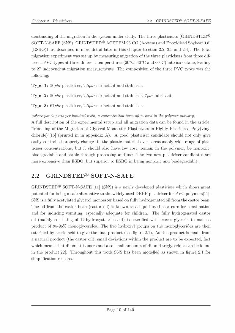
2.4 ESBO
Epoxidised Soybean oil (ESBO, see figure 2.3) is commonly used as the plasticiser for PVC when
the latter is destinated to be used as the lid of jars. ESBO serves a double purpose when added
to the PVC, first of all as plasticiser it makes the polymer more flexible and soft, secondly for
binding any hydrogen chloride released from the PVC during heating by ring opening of the
epoxide (PVC has a tendency to decompose by giving off HCl gas and forming crosslinks among
the polymer chains when HCl leaves. This autocatalytic decomposition occurs at temperatures
near the melting point should be prevented).[9]. ESBO is known for its low migration compared
to other plasticisers, and for this reason it is used in food packaging films and other PVC products
in direct contact with food. The reason for this is to keep the migration of the plasticisers in
the polymer and into the food product within the maximum migration limit of additives[9].
The migration limits set by the European Commission for the use of ESBO is 60mg/kg, and
furthermore there is a limit of 30mg/kg specifically for use in lids of jars containing babyfoods[18].
Figure 2.3: The main component of ESBO.
2.5 DEHP
Di-2-ethylhexyl phtalate (DEHP, see figure 2.4), also sometimes named dioctyl phtalate (DOP),
is by far the most commonly used PVC plasticiser in the world; in 1997 phthalate production
represented 93% of the 900.000 tonnes of plasticisers produced for PVC that year[10]. This is
the reason why this plasticiser is the one against which other plasticisers for PVC are compared
and measured[9].
Page 13 of 140

Chapter 2. Plasticisers 2.5. DEHP
Figure 2.4: Di-2-ethylhexyl phtalate (DEHP)
From the mid 1990’s DEHP came under strong suspicion for being carcinogenic and mutagenic,
which lead to limitations to its use as plasticiser in babytoys (0.04 mg/cm2) in 1998[12], and by
2005 close to a total ban of the product (up to 0.1% in the final product)[27] in the EU. From
2002 the migration from packaging and into foodstuff was also limited by EU legislation[16], and
in 2007 DEHP was only to be used in foodcontact materials as[19]:
a: Plasticiser in repeated use materials and articles contacting non-fatty foods
b: Technical support agent in concentrations up to 0.1 % in the final product
The general systematic migration limit (SML) of DEHP is 1.5 mg/kg food simulant (1.5 ppm).
Along with the implementation of these limitations to the use of DEHP in Europe, a thorough
investigation was conducted by the EU to evaluate the risks of using DEHP. The final risk as-
sessment report was published in 2008[28] with the following general results:
DEHP will not build up in the body, but will be naturally metabolised to mono(2-ethylhexyl)phthalate
(MEHP) and 2 ethylhexanol and excreted from the body mainly through the urine but also fae-
ces. Only very few studies with humans exist. These studies show a somewhat different result,
but in general a half-life of DEHP in the human body from 12 to 48 hours is probably a good
estimate.
As babies have a smaller body mass than adults and as a result a higher exposure ratio of
DEHP, and as they tend to suck and chew on polymer products, many studies have evaluated
the exposure of babies to PVC products containing DEHP. In the risk assessment report a
general worst case exposure for children is set to 0.2 mg/kg·day (sucking and chewing for 3 hours a
day). By monitoring the excretion level of DEHP and its metabolites of a big sample of people
an estimated median intake level of DEHP has been set to 0.0138 mg/kg·day.
The LD50 of DEHP (single dose exposure) is estimated to >10,000mg/kg from experiments with
mice. Repeated dose toxicity tests (2 years with rats) showed toxicity effects to kidneys (increase
of kidney size) which lead to a NOAEL (No Observable Adverse Effect Level) for males at 29
mg/kg·day and 36 mg/kg·day for females.
Page 14 of 140

Chapter 2. Plasticisers 2.5. DEHP
Studies with rodents have shown DEHP to be non-mutagenic, but regarding carcinogenicity a
relevance to humans can not be ruled out, although the evidence is inconclusive. As for repro-
duction concerns a very conservative NOAEL has been set to 4.8 mg/kg·day, based on minimal
testis atrophy at 14 mg/kg·day and complete testis atrophy at 359 mg/kg·day.
Based on these general results, the general conclusion towards consumer risks are[28]:
There is a need for limiting the risks; risk reduction measures which are already
being applied shall be taken into account.
This conclusion is reached because of:� Concerns for children with respect to testicular effects, fertility and toxicity to
kidneys, on repeated exposure, as a consequence of oral exposure from toys and
child-care articles, and multiple routes of exposure.� Concerns for children undergoing long-term blood transfusion and neonates un-
dergoing transfusions with respect to testicular toxicity and fertility, as a con-
sequence of exposure from materials in medical equipment containing DEHP.� Concerns for adults undergoing long-term haemodialysis with regard to repeated
dose toxicity to kidney and testis, fertility, and developmental toxicity, as a
consequence of exposure from materials in medical equipment containing DEHP.
2.5.1 Hansen solubility parameters
For comparison reasons to the calculated Hansen solubility parameters calculated for SNS, these
were also calculated for DEHP. The parameters have been estimated from the group contribution
methodology as proposed by van Krevelen[25] and more recently by Stefanis et al.[26]. The
calculated Hansen solubility parameters calculated by group contribution are listed in table 2.2
together with the parameters found in the official Hansen database[24].
Table 2.2: Calculated Hansen solubility parameters for DEHP using the group con-tribution methods by van Krevelen[25] and Stefanis et al.[26] and parameters from theofficial Hansen database[24] for comparison
[MPa(1/2)] δd δp δh δ
van Krevelen[25]: 17.71 1.84 6.10 18.82Stefanis[26]: 17.54 5.85 1.22 18.53Hansen[24]: 16.60 7.00 3.10 18.28
From table 2.2 it can be seen that the group contribution method captures the dispersive part
(δd) fairly well. Both group contribution methods show problems in estimating the polar (δp) and
the hydrogen bonding part (δh), with the method of Stefanis et al.[26] showing to be the best of
the two for DEHP. The Hansen solubility parameters of DEHP are very similar to the estimated
for SNS (table 2.1), as expected because of the similarities of the two solvents. Furthermore is
Page 15 of 140

Chapter 2. Plasticisers 2.5. DEHP
the method of Stefanis et al.[26] also the one performing best for SNS when comparing to the
similar compounds Hansen solubility parameters.
Page 16 of 140

Chapter 3Diffusion coefficient
The quality of the results from migration modeling are only as good as the parameters used
in the model, i.e. the diffusion and partition coefficients. If experimental migration data exist
for the system of interest, the diffusion coefficient can be obtained by linear regression of the
migration data as a function of the square root of time, eq. 3.1. This very simple correlation
holds however only when there is a big concentration difference of the migrant in the polymer
and the solvent:
Mt = 2Cp0
√
Dt
π⇔ Mt
Cp0=
√D · 2
√
t
π(3.1)
In the linear migration model (eq. 3.1) is Mt [mg/cm2]the migration at time t [s], Cp0 [mg/cm3] is
the initial concentration in the polymer and D [cm2/s ] is the diffusion coefficient. The problem
with this method for estimating the diffusion coefficient is that there must be sufficient available
data points in the early part of the migration, where the concentration difference between the
two layers is very big. Only the four first data points of the seven from the experiment with
Acetem migrating from PVC compound 3 into iso-octane at 20◦C (figure 3.1), clearly lie in the
linear part of the migration, whereas the last three data points show a slower migration than the
correlation (eq. 3.1) predicts. For the same system with SNS as the migrant, six of the seven
data points lie in the linear part.
Page 17 of 140

Chapter 3. Diffusion coefficient
0 100 200 300 400 500 600 700 8000
0.01
0.02
0.03
0.04
0.05
0.06
2q
tπ
Mt/C
p0
(a) SNS
0 100 200 300 400 500 600 700 8000
0.01
0.02
0.03
0.04
0.05
0.06
2q
tπ
Mt/C
p0
(b) Acetem
Figure 3.1: Plots of the linear regression of the data points from the migration of SNSand Acetem from PVC compound 3 at 20◦C into iso-octane used for the estimation ofthe diffusion coefficient through equation 3.1. Only the 4 first data points are used forthe regression in the right figure, whereas 6 out of the 7 data points are used in the leftfigure.
One of the purposes of this project was to estimate the diffusion coefficients of SNS at different
temperatures, based on the migration data from the Danisco experiment. As the migration
experiments conducted by Danisco also included the plasticiser candidate Acetem and the widely
used plasticiser ESBO, the diffusion coefficients were calculated for these plasticisers as well. All
the estimated diffusion coefficients are listed in table 3.1.
Table 3.1: Estimated diffusion coefficients based on equation 3.1 from the Daniscomigration experiment on SNS, Acetem and ESBO from PVC into iso-octane. (datapoints = data points used for linear regression / total number of data points in theexperiment.)
20◦C [cm2
/s ] 40◦C [cm2
/s ] 60◦C [cm2
/s ](data points) (data points) (data points)
SNSPVC type 1 1,30·10−9 (5/7) 1,10·10−9 (4/7) 2,49·10−9 (5/5)PVC type 2 5,95·10−9 (5/7) 5,84·10−9 (5/7) 2,67·10−9 (5/5)PVC type 3 5.93·10−9 (6/7) 5,81·10−9 (4/7) 4,95·10−9 (5/5)
AcetemPVC type 1 6,17·10−9 (7/7) 6,42·10−9 (4/7) 1,07·10−9 (5/5)PVC type 2 1,66·10−8 (5/7) 3,30·10−8 (4/7) 1,49·10−9 (5/5)PVC type 3 3,07·10−8 (4/7) 6,63·10−8 (4/7) 7,67·10−9 (5/5)
ESBOPVC type 1 7,07·10−11 (5/7) 2,43·10−10 (3/6) 6,21·10−10 (5/5)PVC type 2 1,25·10−10 (5/7) 7,25·10−10 (6/7) 8,59·10−10 (4/4)PVC type 3 3,09·10−10 (5/7) 9,47·10−10 (5/7) 1,78·10−9 (4/4)
When diffusion coefficients are needed for temperatures or systems where no experimental data
exist, a theoretical model is then needed. In this work both the polymer-solvent free volume
model of Vrentas and Vrentas[13], and the empirical model by Piringer[14] have been used.
Page 18 of 140

Chapter 3. Diffusion coefficient 3.1. Vrentas and Vrentas Free Volume theory for Diffusion
3.1 Vrentas and Vrentas Free Volume theory for Diffusion
For the estimation of diffusion coefficients in polymer-solvent systems, models based on free
volume theory are widely used, among which the model by Vrentas and Vrentas[13] is probably
the most widely used . This model has shown to be accurate for the estimation of diffusion
coefficients of organic solvent molecules in both rubbery and glassy polymers[14]. A complete
list of symbols for all the expressions used in this section are provided at the end of this thesis.
In all expressions are sub-index 1 used for the solvent and sub-index 2 for the polymer.
By the terminology of Vrentas and Vrentas the solvent self-diffusion coefficient in a rubbery
(above Tg) polymer-solvent system, can be calculated by[13]:
D1 = D0 exp
[
−Ep − Es
RT
]
exp
[
−ω1V∗
1 + ω2ξV∗
2
VFH/γ
]
(3.2)
VFH
γ= ω1
K11
γ1(K21 + T − Tg1) + ω2
K12
γ2(K22 + T − Tg2) (3.3)
The model parameters are: D0, Ep, Es, γ1, γ2,K11,K12,K21,K22, ω1, ω2, Tg1, Tg2, V∗
1 , V ∗
2 , ξ
As it can be seen in equation 3.2 the solvent self-diffusion coefficient by Vrentas and Vrentas[13]
depends on 16 parameters. Though being a large number of parameters it is stated by the authors
that all parameters are physically meaningful (as opposed to the later explained empirical model
by Piringer, eq. 3.27 and 3.28).
For systems where the solvent mass fraction is between 0 to 0.9 (0 < ω1 < 0.9) the polymer
molecule overlap is very much predominant, and for this reason Es can be neglected compared to
Ep in the expression Ep − Es [2]. For simplification reasons and in order to reduce the number
of parameters, many researchers have chosen to set the term Ep − Es equal to zero[4, 29], which
can be the case for many polymer - solvent systems especially at lower temperatures, but is far
from always the case as stated by Macedo and Litovitz [30]. In this work this simplification has
also been used, which means that the expression of the solvent self diffusion coefficient reduces
to:
D1 = D01 exp
(
−(ω1V∗
1 + ξω2V∗
2 )
VFH/γ
)
(3.4)
VFH
γ= ω1
K11
γ1(K21 − Tg1 + T ) + ω2
K12
γ2(K22 − Tg2 + T ) (3.5)
Parameters: D01, ω1, γ1, γ2,K11,K12,K21,K22, ω2, Tg1, Tg2, V∗
1 , V ∗
2 , ξ
Page 19 of 140

Chapter 3. Diffusion coefficient 3.1. Vrentas and Vrentas Free Volume theory for Diffusion
In this more simplified expression of the solvent self diffusion coefficient by Hong[4], only 14
parameters are needed. D01 in the equation of Hong (Eq. 3.4) is equal to D0 when Ep − Es is
set to 0 in the original expression by Vrentas and Vrentas[13], equation 3.2. The determination
of all the parameters needed for the system of SNS in PVC is explained in the following section.
3.1.1 Calculation of parameters of free volume models
D0 and D01 can be calculated by a relationship between viscosity and temperature proposed
by Vrentas[3] derived from a viscosity/self-diffusion relationship by Dullien[31] (Eq. 3.6) and
the solvent self diffusion coefficient expression (eq. 3.2) for the pure solvent, i.e. ω1 = 1 (Eq.
3.7).
ηV D
RT= 0.124 · 10−16V 2/3
c (3.6)
D1 = D0 exp
[
− Es
RT
]
exp
[
− V ∗
1
(K11/γ1)(K21 + T − Tg1)
]
(3.7)
As Es does not change much with temperature, it was chosen by Vrentas to define a new
preexponential diffusion factor in order to decrease the number of parameters − ln D0 ≈ − lnD0+EsRT [3]. With this new average preexponential diffusion factor in the equation it is possible to
determine D0, K11/γ1 and K21 − Tg1 from viscosity/temperature data, by combining eq. 3.6
and eq. 3.7 into eq. 3.8 and using the viscosity/temperature relationship by Vogel[32] (Eq. 3.9).
ln η1 = ln
(
0.124 · 10−16V2/3c,1 RT
M1V01
)
− ln D0 +V ∗
1
(K11/γ1)(K21 + T − Tg1)(3.8)
ln ηi = Ai +Bi
Ci + T(3.9)
Hence (K11/γ1) can be calculated as:
K11/γ1 =V ∗
1
Bi(3.10)
and (K21 − Tg1) as:
K21 − Tg1 = Ci (3.11)
Page 20 of 140

Chapter 3. Diffusion coefficient 3.1. Vrentas and Vrentas Free Volume theory for Diffusion
and D0 as:
D0 =
(
0.124 · 10−16V2/3c,1 RT
M1V 01
)
exp(Ai) (3.12)
From viscosity/temperature data of SNS from Danisco it was possible to obtain a fit to the
expression by Vogel[32] (Eq. 3.9 as shown in figure 3.2. Danisco had two sets of viscosity/tem-
perature data for SNS, and fitting was done using the lsqnonlin function of MATLAB to each set
of data separately and both sets combined. The three sets of parameters did not deviate much
(see figure 3.2), so it was decided to use the combined data for the subsequent calculations.
Figure 3.2: The fitting to the viscosity/temperature data of SNS by the model ofVogel (eq. 3.9). Two sets of experimental data was given by Dansico and the threesets of parameters were obtained by using each set of experimental data or the twocombined. The fitting is done by the lsqnonlin function of MATLAB, which uses alevenberg-marquardt algorithm.
(K12/γ2) and K22 are proposed by Vrentas to be in direct relationship with the WLF constants[1]
by equations 3.13 and 3.14 [33].
K12
γ2=
V ∗
2
2.303Cg1,2C
g2,2
(3.13)
Page 21 of 140

Chapter 3. Diffusion coefficient 3.1. Vrentas and Vrentas Free Volume theory for Diffusion
K22 = Cg2,2 (3.14)
These relationships are derived from the WLF theory[1] by:
log aT = log
(
η
ηg
)
= log
(
Dg
D
)
=−Cg
1 (T − Tg)
Cg2 + T − Tg
(3.15)
From the definition of the self diffusion coefficient for one component (the pure polymer) by
Vrentas[33], it is given that:
ln D = ln D0 −γV ∗
2
K12 (K22 + T − Tg2)(3.16)
Thus:
lnDg
D0= − γV ∗
2
K12 (K22 + Tg2 − Tg2)⇔ (3.17)
lnDg
D0= − γV ∗
2
K12K22(3.18)
By combination of (3.16) and (3.18):
lnDg
D0+ ln
D0
D= − γV ∗
2
K12K22+
γV ∗
2
K12 (K22 + T − Tg2)⇔ (3.19)
lnDg
D=
γV ∗
2 K22 − γV ∗
2 (K22 + T − Tg2)
K12K22 (K22 + T − Tg2)⇔ (3.20)
lnDg
D=
−γV ∗
2 (T − Tg2)
K12K22 (K22 + T − Tg2)⇔ (3.21)
lnDg
D=
− γV ∗
2K12K22
(T − Tg2)
K22 + T − Tg2(3.22)
By comparing (3.22) to the WLF equation (3.15), it can be seen that:
Cg2 = K22 ∧ (3.23)
2.303Cg1 =
γV ∗
2
K12K22⇔ (3.24)
2.303Cg1 Cg
2 =γV ∗
2
K12(3.25)
ω1 is the weight fraction of the solvent in the polymer, hence ω2 (the weight fraction of the
polymer in the solvent) is (1 − ω1). This parameter is kept as the one free parameter that the
Page 22 of 140
Chapter 3. Diffusion coefficient 3.1. Vrentas and Vrentas Free Volume theory for Diffusion
self diffusion should be dependent on.
Tg2 is the glass transition temperature of the polymer and can be found for many polymers in
the literature f.ex. many data are included in the ”Polymer Handbook”[34].
V ∗
1 the specific critical hole free volume, which is the free volume required for a jump of a solvent
molecule. It has been argued by e.g. Vrentas[35] that this volume can be set equal to the specific
occupied volume of solvent at 0K, hence V ∗
1 = V 01 (O). This is also the case of the polymer,
which means that V ∗
2 = (V 02 (O))
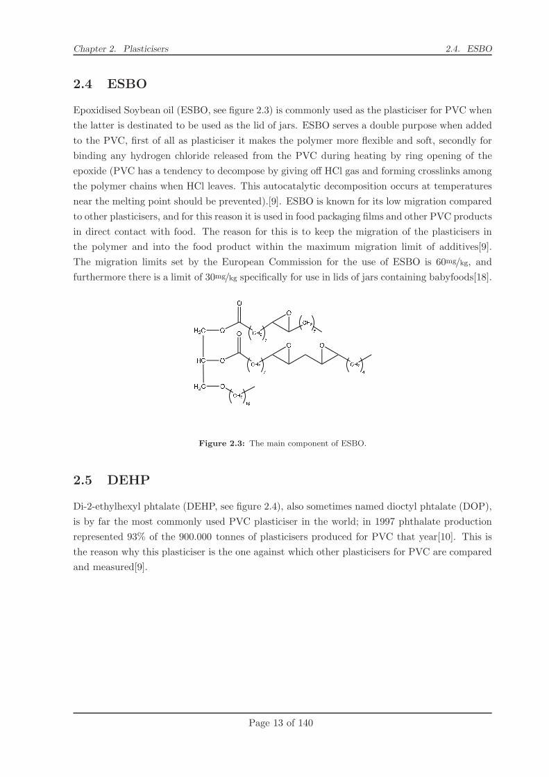
Table 3.2: The calculated parameters used for calculation of the solvent self-diffusioncoefficient (D1) of SNS in PVC by equation 3.4. In the reference column is listed howthe parameters are calculated and the reference.
Parameter value unit Reference
Ep − Es 0.00 [J/mol] [4, 29]K11/γ1 9.66·10−4 [cm3/g·K] visc./temp. data (eq. 3.8)[3]K21 − Tg1 -1.63·102 [K] visc./temp. data (eq. 3.8)[3]K12/γ2 5.44·10−4 [cm3/g·K] WLF (eq. 3.13)[1, 33, 36]K22 3.22·101 [K] WLF (eq. 3.13)[1, 33, 36]Tg2 3.39·102 [K] [34]
V ∗
1 8.22·10−1 [cm3/g] GC model[37]
V ∗
2 6.25·10−1 [cm3/g] [34]
Vc,1 1.61·103 [cm3/g] GC model[38]M1 4.95·102 [g/mol]
V 01 (298K) 9.66·10−1 [cm3/g] GC model[37]
D0/D01 4.68·10−4 [cm2/s] visc./temp. data (eq. 3.8)[3]ω1 3.50·101
ξ 1.31·100 from V ∗
1 and V ∗
2 [4]χ 3.60·10−1 estimate from data by Wang[29]
From the calculated parameters of table 3.2 it is now possible to calculate the solvent self-diffusion
coefficient (D1) using equation 3.4. For the migration modeling it is the polymer/solvent binary
mutual diffusion coefficient that is needed, which can be calculated by equation 3.26[4].
D = D1(1 − φ1)2(1 − 2χφ1) (3.26)
In figure 3.3 an approximated estimate of the Flory-Huggins polymer-solvent interaction pa-
rameter has been used (χ = 0.36)[29] for the calculation of the mutual diffusion coefficient by
equation 3.26. By this method an estimated diffusion coefficient for SNS with a weight ratio of
approximately 0.35 at 298K is 7.0·10−14 cm2/s. The calculated value of SNS from experimental
data as shown in table 3.1 is approximately 6.0·10−9 cm2/s.
Page 23 of 140

Chapter 3. Diffusion coefficient 3.1. Vrentas and Vrentas Free Volume theory for Diffusion
0 0.1 0.2 0.3 0.4 0.5 0.6 0.7 0.8 0.9 110
−50
10−45
10−40
10−35
10−30
10−25
10−20
10−15
10−10
10−5
100
solvent weight fraction ω1
D [c
m2 /
s]
D
1
D
Figure 3.3: Estimated solvent self-diffusion coefficient (D1, eq 3.4) and the solventdiffusion coefficient from the Vrentas/Duda free volume model.
3.1.2 Conclusion
This complex model by Vrenta and Vrentas contains 7 to 12 physical parameters depending on
how they are defined. The results shows for this specific case that the model under predict the
experimentally derived mutual diffusion coefficients of this highly plasticised PVC. As highly
plasticised PVC is a complex system, there is no guarantee that the experimentally derived
diffusion coefficient is physically meaningful. But a system is never stronger that its weakest
point. In this case the model uses up to 12 physically meaningful parameters, but many of
these parameters are at best derived from fitting to experimental data and in many cases from
group contribution models. This results in low predictive power for the model. Many of these
estimated physically meaningful parameters for each of the pure components could just as well
be grouped to one or two non-physical meaningful parameters fitted to one set of experimental
data. Moreover, the estimated value of ξ is larger than 1, meaning that the jumping unit of the
solvent (SNS) is larger than the jumping unit of the polymer for this system. To conclude, this
Page 24 of 140

Chapter 3. Diffusion coefficient 3.2. Empirical diffusion coefficient estimation
free volume model does not perform well for systems where ξ is larger than 1, i.e. for diffusion of
very large organic molecules. The scope of this work has been to develop a simple method to be
used by the industry (in this case specifically by Danisco) able to obtain accurate and reliable
migration data, which proved to be very hard with the previously examined free volume model.
3.2 Empirical diffusion coefficient estimation
In 2003 a simplified, empirical approach to obtain diffusion coefficients for the migration mod-
eling was approved in EU, for the cases where only little or none data exist for the system of
interest. The model that was approved for this use, was the semi-empirical model proposed by
Otto Piringer for safe over estimation of diffusion coefficients[14]. Safe over estimation means
that the model is optimized to predict or overpredict at least 95% of the diffusion coefficient
data that was used for the development of the model. The aim when developing the specific
model has been to make a reliable model with as few as possible parameters, easy to use for
industrial applications. The model is only dependent on three parameters: a purely empirical
collective polymer specific parameter (Ap), the molecular weight of the migrant (Mr) and the
temperature (T ).
From the migration experiments of Danisco it was only the data of the ESBO plasticiser that
followed the Arrhenius correlation. For this reason it was chosen to use only these data in order
to find the polymer specific parameter Ap for the three PVC types in the study. In the book
by Piringer[14] two versions of the diffusion coefficient estimation model (3.27 and 3.28) are
presented:
Dp = 104 exp
(
Ap − 0.01Mr −10454
T
)
(3.27)
Dp = 104 exp
(
(
A′
p −τ
T
)
− 0.1351M2/3r + 0.003Mr −
10454
T
)
(3.28)
3.2.1 Ap by equation 3.27
From the experimentally derived diffusion coefficients of ESBO in the three compounds it is
possible to get the Ap value for each experiment when the molecular weight of the migrant is
known. Table 3.3 shows the values and the mean values for the different PVC types:
Table 3.3: Experimentally derived Ap values for ESBO in PVC by equation 3.27, usingthe diffusion coefficients from table 3.1, temperature and the molecular weight of ESBO(Mr = 905g/mol)
20◦C 40◦C 60◦C Mean Ap
Type 1 12.13 11.09 10.02 11.08Type 2 12.70 12.18 10.34 11.74Type 3 13.60 12.44 11.07 12.37
Page 25 of 140

Chapter 3. Diffusion coefficient 3.2. Empirical diffusion coefficient estimation
When the diffusion takes place in PVC it is suggested by Piringer to use only equation 3.27, but
as it can be seen in figure 3.4, the Ap values seem to be dependent on temperature as well.
290 295 300 305 310 315 320 325 330 33510
10.5
11
11.5
12
12.5
13
13.5
14
Temp [K]
Ap
Figure 3.4: Ap mean value for each PVC type by equation 3.27. (black=type 1,red=type 2, blue=type 3)
3.2.2 Ap by equation 3.28
As for equation 3.27 the Ap value can be estimated for all the PVC types and temperatures of
ESBO (see table 3.4).
Table 3.4: Experimentally derived Ap values for ESBO in PVC by equation 3.28 usingthe diffusion coefficients from table 3.1, temperature and the molecular weight of ESBO(Mr = 905g/mol).
20◦C 40◦C 60◦C
Type 1 13.00 11.96 10.89Type 2 13.57 13.05 11.22Type 3 14.48 13.32 11.95
From these Ap values the two polymer parameters of equation 3.28 can be calculated by linear
regression (Ap = A′
p − τT , see table 3.5). This gives a satisfactory fit of the model to the experi-
mentally derived Ap values (see figure 3.5).
Page 26 of 140

Chapter 3. Diffusion coefficient 3.2. Empirical diffusion coefficient estimation
290 295 300 305 310 315 320 325 330 33510.5
11
11.5
12
12.5
13
13.5
14
14.5
15
Temp [K]
Ap
Figure 3.5: Ap now also dependent of temperature`
Ap = A′
p −τT
´
for each compoundby equation 3.28. (black=type 1, red=type 2, blue=type 3)
The fitted parameters for equation 3.28 are presented in table 3.5:
Table 3.5: The fitted polymer parameters of equation 3.28, and the collected Arrheniusactivation energy EA = (10454 + τ )R.
A′
p τ EA
[kJ/mol]
Type 1 -4.5 -5140 44.16Type 2 -5.5 -5667 39.78Type 3 -6.5 -6160 35.68
Page 27 of 140

Chapter 3. Diffusion coefficient 3.2. Empirical diffusion coefficient estimation
3.2.3 Estimation of diffusion coefficients by equations 3.27 and 3.28
290 295 300 305 310 315 320 325 330 335−11
−10.5
−10
−9.5
−9
−8.5
−8
Temp [K]
Log(
D)
Figure 3.6: Estimation of the diffusion coefficients for ESBO in the three PVC com-pounds (black=type 1, red=type 2, blue=type 3). The dotted line corresponds to equa-tion 3.27 results, and the filled corresponds to equation 3.28results .
As it can be seen in figure 3.6 there is no doubt that equation 3.28 correlates more accurately
the experimental data. In the book by Piringer[14] the listed Ap value for PVC (T < 70◦C) has
a value of -4, which is very far from the value of Ap estimated here, which is in the area of 11 to
13. This is because the value for PVC in the Piringer book corresponds to empty and very rigid
PVC. The ”high” loading of plasticiser in the PVC in the experiments performed by Danisco
makes the polymer much more flexible, hence a totally different specific polymer parameter is
obtained. The results from this work have been confirmed by Otto Piringer himself as being
very plausible (by private communications in 2008).
Once these polymer specific parameters have been obtained, it should be possible to estimate
the diffusion coefficients for the two other plasticisers (SNS and Acetem), knowing that ESBO
has a molecular weight of 905 g/mol, SNS of 500 g/mol and Acetem of 330 g/mol. The estimation
for each of the three PVC types can be seen in figures 3.7 and 3.8.
Page 28 of 140

Chapter 3. Diffusion coefficient 3.2. Empirical diffusion coefficient estimation
300 400 500 600 700 800 900 1000−11
−10.5
−10
−9.5
−9
−8.5
−8
−7.5
−7
−6.5
−6
Mr
Log(
D)
(a) PVC type 1
300 400 500 600 700 800 900 1000−11
−10
−9
−8
−7
−6
−5
Mr
Log(
D)
(b) PVC type 2
Figure 3.7: The estimation of the diffusion coefficient for PVC Type 1 and 2. Dashedline is obtained with eq. 3.27 and solid line is obtained with eq. 3.28. (black=20◦C,red=40◦C, blue=60◦C)
300 400 500 600 700 800 900 1000−10.5
−10
−9.5
−9
−8.5
−8
−7.5
−7
−6.5
−6
−5.5
Mr
Log(
D)
Figure 3.8: he estimation of the diffusion coefficient for PVC Type 3. Dashed line isobtained with eq. 3.27 and solid line obtained is with eq. 3.28. (black=20◦C, red=40◦C,blue=60◦C)
From figures (3.7, 3.8) it is clear that the diffusion coefficients obtained experimentally (by the
linear model, eq. 3.1) for SNS and Acetem at 40◦C and 60◦C are not as high as predicted by
the Piringer model. This is thought to be because of the fast depletion of plasticisers from the
outer area of the polymer, which gives a much lower diffusion through this more rigid PVC area.
This partly depleted PVC polymer will then have a much different average mutual diffusion
coefficient of the system. This is explained in more detail in section ”Diffusion Coefficients from
Experimental Data” in the article: ”Modeling of the Migration of Glycerol Monoester Plasticisers
in Highly Plasticised Poly(vinyl chloride)”[15], printed in appendix A. Moreover, it is clear that
equation 3.28 makes the best fit also at higher molecular weights. Table 3.6 lists the estimated
diffusion coefficients at 20◦C of SNS, Acetem, ESBO and DEHP.
Page 29 of 140

Chapter 3. Diffusion coefficient 3.3. Concentration dependent diffusion coefficient
Table 3.6: Diffusion coefficients estimated (Dcalc by equation 3.28) and from experi-mentally data (Dexp) for SNS, Acetem, ESBO and DEHP in PVC at 20◦C. PVC type1,2,3 are almost the same PVC compound only with minor changes to the ratio of thedifferent additives in the final PVC compound (see section 2.1).
PVC type 1 PVC type 2 PVC type 3Mw Dcalc Dexp Dcalc Dexp Dcalc Dexp
[g/mol] [cm/s2]·10−10 [cm/s2]·10−10 [cm/s2]·10−10
Acetem 330 62.68 61.66 139.32 166.01 275.71 307.36DEHP 390 35.10 78.00 154.36SNS 500 13.32 13.00 29.59 59.54 58.56 74.30ESBO 905 0.72 0.71 1.60 1.25 3.18 3.09
This methodology of estimating diffusion coefficients was used for the approval of SNS as plasti-
ciser in Polyethylene terephthalate (PET) polymers by the American Food and Drug Adminis-
tration (FDA) in 2009. The calculations was done using equation 3.28 with the specific polymer
parameters of A′
p = 6.0 and τ = 1577 as suggested by Begley et al.[39]. The calculated diffusion
coefficients of SNS in PET by this method are: Dcalc(20◦C) = 2.53·10−10 cm2/s; Dcalc(40
◦C) =
17.54·10−10 cm2/s; Dcalc(60◦C) = 96.33·10−10 cm2/s.
3.2.4 Conclusion
The fully estimated diffusion coefficients of SNS and Acetem at 20◦C are very close to those
experimentally derived. This shows the capability of this very simple model to give fairly good
estimates of diffusion coefficients of similar migrants in the same polymer. The problem of over
prediction of diffusion coefficients at the higher temperatures is probably related to the change
of the polymer physics of the system due to fast depletion of plasticisers[15].It seems that the
model is very applicable for the specific use of getting good and fast estimates of the diffusion
coefficients.
3.3 Concentration dependent diffusion coefficient
Normally for migration modeling the Diffusion coefficient (D) is seen as concentration indepen-
dent, which in most cases is acceptable. But for highly plasticised Polyvinyl Chloride (PVC),
where the plasticisers migrates away from the polymer this concentration independence of the
diffusion coefficient is not feasible any more. It is proposed that the diffusion coefficient in PVC
can change from 10−7 cm2/s in fully plasticised PVC to around 10−16 cm2/s in depleted, rigid
PVC[14]. This large span has to be implemented in the migration model in some way. As the
migration is solved by fem methodology it is proposed to let the diffusion coefficient between
each mesh point be a function of the local concentration. Three functions for this dependence
is proposed:
Page 30 of 140

Chapter 3. Diffusion coefficient 3.3. Concentration dependent diffusion coefficient
Model 1:
D =
(
Ct
C0
)w
(Dhigh − Dlow) + Dlow (3.29)
Model 2:
log D =
(
Ct
C0
)w
(log Dhigh − log Dlow) + log Dlow (3.30)
where D is the calculated diffusion coefficient; Dlow is the diffusion coefficient in rigid PVC;
Dhigh is the diffusion coefficient in fully plasticised PVC; Ct is the local concentration of plasti-
ciser at time t; C0 is the concentration of plasticiser at the beginning or when fully plasticised
and w is the fitting parameter going from 0 to 1000 for model 1 and from 0 to 100 for model 2
(see figure 3.9).
These two models (eq. 3.29 and 3.30) are simply the completely linear relationship between
the two outer points of the diffusion coefficient function (Dlow is rigid and Dhigh fully plasti-
cised PVC). Model 2 is the same as model 1 but the two outer points are represented as the
logarithm of the diffusion coefficients. For both models the boundary conditions are fulfilled
(Ct
C0= 0 → D = Dlow and Ct
C0= 1 → D = Dhigh). Plots of model 1 and 2 can be seen in figure
3.9, using some arbitrary model parameters covering most of the parameters space.
0 0.1 0.2 0.3 0.4 0.5 0.6 0.7 0.8 0.9 110
−16
10−15
10−14
10−13
10−12
10−11
10−10
10−9
10−8
10−7
C0 / C
t
D
(a) Model 1 (eq. 3.29)
0 0.1 0.2 0.3 0.4 0.5 0.6 0.7 0.8 0.9 110
−16
10−15
10−14
10−13
10−12
10−11
10−10
10−9
10−8
10−7
C0 / C
t
D
(b) Model 2 (eq. 3.30)
Figure 3.9: Plot of D as function of the local concentration when changing the wparameter for model 1 (left, w=[0.1, 1, 5, 10, 20, 50, 100, 1000]) and model 2 (right,w=[0.1, 0.2, 0.5, 1, 2, 5, 10, 100]). For reference in all graphs are plotted model 1(w=10), model 2 (w=1) and model 3 (w=0.6; p=100).
Model 3:
D = Dlow +Dhigh
1 + exp(
p(
w − CtC0
)) (3.31)
where D is the calculated diffusion coefficient; Dlow is the diffusion coefficient in rigid PVC;
Page 31 of 140

Chapter 3. Diffusion coefficient 3.3. Concentration dependent diffusion coefficient
Dhigh is the diffusion coefficient in fully plasticised PVC; Ct is the local concentration of plas-
ticiser at time t; C0 is the concentration of plasticiser at start or when fully plasticised and w
and p are fitting parameters going from 0 to 1 or 1 to 1000 respectively.
Model 3 (plotted in figure 3.10) is derived after discussing with professor Ole Hassager from the
Danish Polymer Centre, Department of Chemical and Biochemical Engineering, DTU. If the
concentration of the plasticiser is lowered in the polymer, then the glass transition temperature
(Tg) will rise (the opposite of plasticisation of the polymer). At some stage as the concentration
of the plasticiser changes Tg will be equal to the temperature of the system (T ), if the system
is at ambient temperature. At this point a big change of the diffusion coefficient is expected.
Model 3 can mimic such a sudden change between the two outer values. The boundary condi-
tions are not fulfilled as such in model 3, and some further derivations have to be done. Two new
terms are introduced, Dempty (true diffusion coefficient at empty PVC) and Dfull (true diffusion
coefficient at fully plasticised PVC)
Boundary Condition 1, (CtC0
= 0 → D = Dempty):
Dempty = Dlow +Dhigh
1 + exp (p (w − 0))⇔
Dlow = Dempty −Dhigh
1 + exp (pw)(3.32)
Boundary Condition 2, (CtC0
= 1 → D = Dfull):
Dfull = Dlow +Dhigh
1 + exp (p (w − 1))⇒ using Boundary Condition 1, eq. 4
Dfull = Dempty −Dhigh
1 + exp (pw)+
Dhigh
1 + exp (p (w − 1))⇔
Dfull − Dempty = Dhigh
( −1
1 + exp (pw)+
1
1 + exp (p (w − 1))
)
⇔
Dhigh =Dfull − Dempty1
1+exp(p(w−1)) −1
1+exp(pw)
(3.33)
This means that model 3 (eq. 3.31) with the right boundary conditions (eq. 3.32 and 3.33) will
be:
Model 3:
D = Dempty −Dfull−Dempty1
1+exp(p(w−1))−
11+exp(pw)
1 + exp (pw)+
Dfull−Dempty1
1+exp(p(w−1))−
11+exp(pw)
1 + exp(
p(
w − CtC0
)) ⇔ (3.34)
D = Dempty +Dfull − Dempty1
1+exp(p(w−1)) − 11+exp(pw)
1
1 + exp(
p(
w − CtC0
)) − 1
1 + exp (pw)
Page 32 of 140

Chapter 3. Diffusion coefficient 3.3. Concentration dependent diffusion coefficient
0 0.1 0.2 0.3 0.4 0.5 0.6 0.7 0.8 0.9 110
−16
10−15
10−14
10−13
10−12
10−11
10−10
10−9
10−8
10−7
C0 / C
t
D
Figure 3.10: Plot of D as function of the local concentration when changing the wparameter (w=[0.2, 0.4, 0.6, 0.8, 1.0], the full line with p=100) and the p parameter(p=[1, 10, 20, 50, 100, 1000], broken lines with w=0.6) for model 3 (eq. 3.31). Forreference in all graphs are plotted model 1 (w=10), model 2 (w=1) and model 3 (w=0.6;p=100).
Finally, an analytical model with a concentration independent diffusion coefficient which in ear-
lier investigations showed capabilities to mimic the slower migration along with the depletion of
the plasticiser from the polymer was also tested against the migration data[15]. This model was
originally developed by Kondyli et al.[40] for migration into more or less agitated solutions. In
this model (named model 4) the fitting is done on the agitation parameter ”u”, and this model
is not solved by the fem methodology but by calculating the migration as a function of time t.
Model 4:
Mt
M∞
=ut
2Lerf
(
ut
2√
Dt
)
ut − L
2Lerf
(
L − ut
2√
Dt
)
+1
2
+
√Dt
L√
π
{
exp
[
−(ut)2
4Dt
]
− exp
[
−(L − ut)2
4Dt
]}
(3.35)
With the migration data at 20◦C it was possible with the normal concentration independent
diffusion coefficient to obtain fairly good correlation to the experimental data[15], but this was
not possible at 40◦C and at 60◦C. This investigation around concentration-dependent diffusion
coefficient modeling aims at finding better methods for the estimation of migration data at 40◦C
and 60◦C, but of course all available data were used. From the same migration data as used
in this investigation the polymer specific parameters for the Piringer model[14] for diffusion
coefficient estimation have been found[15]. These parameters can be seen in table 3.4.
In the fitting calculations the diffusion coefficient of the empty, rigid PVC (Dlow or Dempty) was
set to the same value calculated by equation 3.27 using the polymer specific parameters given
by Piringer for rigid PVC (Ap = −4), which give diffusion coefficients in the order of ∼ 10−17
cm2/s. For the diffusion coefficient of the fully plasticised PVC (Dhigh or Dfull) three different
Page 33 of 140

Chapter 3. Diffusion coefficient 3.3. Concentration dependent diffusion coefficient
values where used.
DAp Calculated with eq. 3.27 using an Ap value of 14.
DAp2 Calculated with eq. 3.28 using an Ap value of 20 and τ = 1577.
Dest Calculated with eq. 3.28 using data from table 3.4.
The fitting was done via the optimisation functions in MatLab (R2008a) called ”lsqnonlin”and
”fmincon”. The objective function used is:
feval =n∑
t=1
(
xt − Mt
xt
)2
(3.36)
where xt is migration measured at time t, Mt is the estimated migration at time t, and n is the
number of samples (here 7).
3.3.1 Results
SNS
As it can been seen in table 3.7, model 4 (the analytical model by Kondyli et al. eq. 3.35) is
not very accurate at 40◦C and especially at 60◦C. Furthermore, the agreement when using DAp2
or DAp, which are diffusion coefficients with no use of experimental data, is very poor. When
comparing models 1-3 (the models with concentration dependent diffusion coefficient) it is clear
that there is no significant difference in the results when using Dest, DAp2 or DAp. Should one be
chosen, it must be DAp2 when looking at all three temperatures. In the same way the difference
between using models 2 or 3 is very small, although these two models are somewhat better than
model 1.
Table 3.7: The optimal value of the objective function (feval in eq. 3.36) for all the
experiments with SNS. The value is muliplied with 100 for easier reading of the table.
For each experiment the best fit is indicated with bold letters.
Temp Compound Model Dest DAp2 DAp
(lsq) (fmin) (fmin) (fmin)
20◦C 1 1 109 109 87 33
2 110 110 88 35
3 138 109 63 38
4 991 995 31 4061
2 1 505 505 8 26
2 505 505 8 24
3 716 508 6 34
4 882 882 355 163
Page 34 of 140

Chapter 3. Diffusion coefficient 3.3. Concentration dependent diffusion coefficient
table 3.7 – continued
Temp Compound Model Dest DAp2 DAp
(lsq) (fmin) (fmin) (fmin)
3 1 75 75 43 13
2 75 75 43 12
3 160 85 43 22
4 654 654 580 47
40◦C 1 1 185 185 6958 3364
2 186 186 121 155
3 180 179 127 191
4 141 141 29170 66026
2 1 96 96 60 194
2 97 97 50 165
3 77 77 42 450
4 472 472 1380 5583
3 1 204 206 63 107
2 207 206 63 86
3 132 132 60 124
4 304 304 788 3633
60◦C 1 1 13 13 4947 173
2 13 13 82 132
3 15 15 96 140
4 91 91 129254 178930
2 1 75 76 39 4739
2 74 74 36 41
3 83 83 41 61
4 516 516 75702 103966
3 1 57 57 61 4990
2 58 58 54 76
3 59 59 67 103
4 296 296 38900 54820
With this knowledge when looking at table 3.8 with the optimal parameters of the models, it
is clear that by average the optimal p parameters for model 3 is around 20. this means that
Page 35 of 140

Chapter 3. Diffusion coefficient 3.3. Concentration dependent diffusion coefficient
the optimal slope of model 3 (see figure 3.10) is almost the same as for models 1 and 2. It was
hoped that when making the calculated diffusion coefficient a function of the temperature (Dest,
DAp2 or DAp) it would be possible to obtain a good average parameter from the fitting at the
different temperatures. But as it can be seen the optimal parameters for models 2 and 3 (the
w parameter) are not the same for the three temperatures. This is not even the case within the
same temperature where the optimal parameter deviates significantly between the three PVC
types.
Table 3.8: The optimal parameters (w and p) for SNS for models 1-3. For model 4 the
optimal agitation parameter u is listed in the w column and it is multiplied with 105.
Temp Compound Model Dest DAp2 DAp
(lsq) (fmin) (fmin) (fmin)
w p w p w p w p
20◦C 1 1 0.02 0.02 1.74 4.68
2 0.00 0.00 0.11 0.28
3 0.03 20 0.00 120 0.55 20 0.77 20
4 7.23 6.77 0.15 0.00
2 1 0.00 0.00 0.10 1.51
2 0.00 0.00 0.01 0.09
3 0.01 20 0.00 1000 0.00 20 0.64 5
4 38.68 38.92 36.61 26.80
3 1 0.00 0.00 0.00 1.22
2 0.00 0.00 0.00 0.07
3 0.01 20 0.00 121 0.00 431 0.50 7
4 39.98 39.96 39.90 34.14
40◦C 1 1 1.58 1.58 72.42 38.69
2 0.12 0.12 0.69 1.03
3 0.53 20 0.53 20 1.00 15 1.00 22
4 0.00 0.00 0.00 0.00
2 1 0.25 0.25 3.39 6.06
2 0.02 0.02 0.22 0.37
3 0.13 20 0.13 20 1.00 6 0.82 20
4 31.59 31.56 0.00 0.00
Page 36 of 140

Chapter 3. Diffusion coefficient 3.3. Concentration dependent diffusion coefficient
table 3.8 – continued
Temp Compound Model Dest DAp2 DAp
(lsq) (fmin) (fmin) (fmin)
w p w p w p w p
3 1 0.74 0.74 3.24 5.66
2 0.05 0.05 0.21 0.35
3 0.32 20 0.32 20 0.85 7 0.89 12
4 27.51 27.36 0.15 0.00
60◦C 1 1 1.79 1.79 72.42 32.09
2 0.15 0.15 1.61 1.92
3 0.57 20 0.57 20 1.00 31 0.99 40
4 0.00 0.00 0.00 0.00
2 1 2.36 2.38 19.69 65.21
2 0.19 0.19 1.30 1.67
3 0.63 20 0.63 20 1.00 27 0.99 35
4 0.00 0.00 0.00 0.00
3 1 2.20 2.20 14.85 154.03
2 0.17 0.17 0.97 1.27
3 0.62 20 0.62 20 1.00 21 1.00 27
4 0.00 0.00 0.00 0.00
In figure 3.11 are shown two examples for the best fit of the models to SNS migration from PVC
type 3 at 40◦C and 60◦C. The models are compared to the estimated migration by the analytical
solution of Crank[41] with the calculated diffusion coefficient from the first 5 data points (Dexp).
Page 37 of 140

Chapter 3. Diffusion coefficient 3.3. Concentration dependent diffusion coefficient
0 1000 2000 3000 4000 5000 60000
0.1
0.2
0.3
0.4
0.5
0.6
0.7
0.8
0.9
1
minutes
Ct /
C0
Crank with DexpCrank with DfullCrank with DemptyModel 1, Fval=0.062759Model 2, Fval=0.063313Model 3, Fval=0.060236Model 4, Fval=0.78806
0 100 200 300 400 5000
0.1
0.2
0.3
0.4
0.5
0.6
0.7
0.8
0.9
1
minutes
Ct /
C0
Crank with DexpCrank with DfullCrank with DemptyModel 1, Fval=0.060887Model 2, Fval=0.054386Model 3, Fval=0.066713Model 4, Fval=38.9001
Figure 3.11: Migration estimated with the optimal parameter fitting results (listed intable 3.10) of the 4 models for SNS in PVC type 3 at 40◦C (left) and 60◦C (right) usingDAp2. Also in the figure is plotted the migration using the analytical migration modelof Crank (eq. 4.1 using the three diffusion coefficients Dempty , Dexp, Dfull.
Acetem
As for SNS, model 4 performs poorly compared to the other models at 60◦C (see table 3.9).
When comparing the other three models over all temperatures it is seen that, as for SNS, mod-
els 2 and 3 perform somewhat better than model 1. For Acetem using Dest and DAp2 in models
1 and 2 the results are overall about equally good.
Table 3.9: The optimal value of the objective function (feval in eq. 3.36) for all the
experiments with Acetem. The value is muliplied with 100 for easier reading of the table.
For each experiment the best fit is indicated with bold letters.
Temp Compound Model Dest DAp2 DAp
fmin fmin fmin
20◦C 1 1 130 264 617
2 130 255 585
3 134 285 631
4 185 825 7570
2 1 67 78 284
2 67 78 261
3 70 140 236
4 108 24 1603
Page 38 of 140

Chapter 3. Diffusion coefficient 3.3. Concentration dependent diffusion coefficient
table 3.9 – continued
Temp Compound Model Dest DAp2 DAp
fmin fmin fmin
3 1 43 38 36
2 43 38 31
3 40 31 45
4 166 141 179
40◦C 1 1 165 231 455
2 170 186 368
3 102 193 436
4 153 7061 13533
2 1 132 128 422
2 132 105 345
3 73 83 715
4 214 1031 2604
3 1 252 108 152
2 252 116 136
3 238 105 131
4 305 178 394
60◦C 1 1 3251 300 186
2 52 187 1368
3 51 143 160
4 37257 658300 768552
2 1 4647 64 4951
2 128 56 351
3 125 68 71
4 25051 221284 256737
3 1 405 4658 479
2 407 444 468
3 430 473 480
4 8082 54238 63394
When looking at the optimal parameters found for Acetem (table 3.10) there is no tendency
towards one optimal p parameter when looking at DAp2. When Dest is used the value p=20
is again the optimal value, as for SNS. As for SNS, there are no overall best w parameters for
Page 39 of 140

Chapter 3. Diffusion coefficient 3.3. Concentration dependent diffusion coefficient
models 2 and 3, not even at each temperature.
Table 3.10: The optimal parameters (w and p) for Acetem for models 1-3. For model 4
the optimal agitation parameter u is listed in the w column and is multiplied with 105.
Temp Compound Model Dest DAp2 DAp
(fmin) (fmin) (fmin)
w p w p w p
20◦C 1 1 0.10 1.89 5.56
2 0.01 0.12 0.34
3 0.00 20 0.73 6 0.94 10
4 44.98 19.79 0.00
2 1 0.00 0.63 2.79
2 0.00 0.04 0.17
3 0.00 75 0.28 20 1.00 5
4 116.43 92.85 44.06
3 1 0.00 0.05 1.58
2 0.00 0.00 0.09
3 0.02 638 0.00 20 0.65 6
4 186.11 183.41 135.27
40◦C 1 1 1.12 7.51 12.19
2 0.09 0.50 0.77
3 0.42 20 1.00 11 1.00 17
4 24.00 0.00 0.00
2 1 0.30 3.31 6.06
2 0.02 0.22 0.37
3 0.17 20 1.00 6 0.81 15
4 159.96 112.19 82.73
3 1 0.00 1.85 3.56
2 0.00 0.12 0.22
3 0.05 20 0.59 9 1.00 7
4 424.77 261.22 347.51
60◦C 1 1 33.60 42.05 49.85
2 0.86 3.61 3.47
3 0.92 20 1.00 53 1.00 59
4 0.00 0.00 0.00
Page 40 of 140

Chapter 3. Diffusion coefficient 3.3. Concentration dependent diffusion coefficient
table 3.10 – continued
Temp Compound Model Dest DAp2 DAp
(fmin) (fmin) (fmin)
w p w p w p
2 1 49.85 37.70 109.59
2 0.78 2.94 2.95
3 0.91 20 1.00 47 1.00 52
4 0.00 0.00 0.00
3 1 6.11 65.21 32.09
2 0.50 1.80 2.25
3 0.83 20 0.99 35 1.00 40
4 0.00 0.00 0.00
In figure 3.12 are shown two examples given for the best fit of the models to Acetem migration
from PVC type 3 at 40◦C and 60◦C. The models are compared to the estimated migration
by the analytical solution of Crank[41] with the calculated diffusion coefficient based on the
first 5 data points (Dexp). As it can be seen the quality of experimental migration data is not
very good in all cases , fact which partly explains the somewhat poor performance of the models.
0 1000 2000 3000 4000 5000 60000
0.2
0.4
0.6
0.8
1
1.2
1.4
minutes
Ct /
C0
Crank with DexpCrank with DfullCrank with DemptyModel 1, Fval=0.10758Model 2, Fval=0.11605Model 3, Fval=0.10517Model 4, Fval=0.17802
0 100 200 300 400 5000
0.1
0.2
0.3
0.4
0.5
0.6
0.7
0.8
0.9
1
minutes
Ct /
C0
Crank with DexpCrank with DfullCrank with DemptyModel 1, Fval=0.064158Model 2, Fval=0.056461Model 3, Fval=0.067853Model 4, Fval=221.2839
Figure 3.12: Migration estimated with the optimal parameter fittings (listed in table3.10) of the 4 models for Acetem in PVC type 3 at 40◦C (left) and PVC type 2 60◦C(right) using DAp2. Also in the figure is plotted the migration using the analyticalmigration model of Crank using the three diffusion coefficients Dempty , Dexp, Dfull.Especially on the left plot the scattering of the experimental migration data can beclearly seen.
Page 41 of 140

Chapter 3. Diffusion coefficient 3.3. Concentration dependent diffusion coefficient
3.3.2 Conclusion
The main conclusion from this investigation is that no new final model with physically mean-
ingfull parameters has been found, able to correlate satisfactorily the migration data of the
plasticisers in highly plasticised PVC. However, when compared to the proposed best migration
model with concentration independent diffusion coefficient (model 4, eq. 3.35), all three new
suggested models perform better with optimised parameters. Models 2 and 3 seem to perform
overall slightly better than model 1, and DAp2 is the best function to use for calculating the
diffusion coefficient of the fully plasticised PVC as a function of temperature.
0 0.1 0.2 0.3 0.4 0.5 0.6 0.7 0.8 0.9 10
0.1
0.2
0.3
0.4
0.5
0.6
0.7
0.8
0.9
1x 10
−7
C0 / C
t
D
0 0.1 0.2 0.3 0.4 0.5 0.6 0.7 0.8 0.9 110
−16
10−15
10−14
10−13
10−12
10−11
10−10
10−9
10−8
10−7
C0 / C
t
D
Figure 3.13: Plot of the overall optimal parameters for model 2 (w=[0.00 0.05, 0.17],at 20◦C, 40◦C, 60◦C respectively) and for model 3 (p=20; w=[0.01 0.3, 0.6], at 20◦C,40◦C, 60◦C respectively). The left figure is with linear scale of the diffusion coefficientand the right is with logarithmic scale. For both models is the plot of the function goingtowards the lower right corner as the temperature rise. Especially on the logarithmicplot (right) it can be seen that the optimal function for the two models lies fairly close ateach temperature; 20◦C corresponds to the two plots most up in the top left corner, 40◦Ccorresponds to the next two and 60◦C corresponds to the ones furthest down towardsthe middle of the graph.
The optimum parameters of models 2 and 3 are shown in figure 3.13 and as it can be seen, the
optimal functions, when going from Dempty to Dfull, are fairly close to each other for the two
models at all three temperatures examined.
Page 42 of 140

Chapter 4Migration
In this work the focus has been so far to accurately predict migration of additives in a polymer
and into food (often as migration from food packaging), in order to comply with the systematic
migration limits (SML) set by EU[12, 16–20] as described in chapter 2. For simplification and
unification of the experimental work and/or calculations that have to be done in order to get
a product approved by the legislation, four food simulants have been chosen by the European
Commision[12]:
(A) Distilled water
(B) 3% Acetic Acid (weight/volume)
(C) 10% Ethanol (volume/volume)
(D) Olive oil or Sunflower oil (in some cases Iso-octane)
In the specific case of milk and similar products, it is suggested to use 50% ethanol as the food
simulant.
For systems with a low concentration of the additive in the polymer and consisting of only
one polymer layer, this migration can be solved analytical by the solution of Fick’s second law
of diffusion as done by Crank in his book: ”Mathematics of diffusion”[41]. Equation 4.1 is the
solution by Crank for the simple system of migration from a polymer layer and into a solvent,
which also is the solution suggested by Piringer for this system[14].
Mt
M∞
= 1 −∞∑
n=1
2α (1 + α)
1 + α + α2q2n
exp
(−Dtq2n
L2
)
(4.1)
where Mt is the migration at time t, M∞ is the migration at infinite time, D the diffusion
coefficient, L is the thickness of the polymer and qn is the positive roots of [tan qn = −αqn]. α
is a dimensionless quantity taking the solubility of the migrant in the solvent and the volume
ratio of the polymer to the solvent into account. α = 1K
VsVp
, where VsVp
is the volume ratio of the
Page 43 of 140

Chapter 4. Migration
solvent over the polymer and K is the partition coefficient of the migrant in the polymer over
the solvent, K =Cp,∞
Cs,∞.
For highly plasticised PVC, the concentration of the migrant (the plasticiser itself) is so high,
that the depletion of the plasticiser from the polymer effects the structural behavior of the
polymer. Such system are not readily solved by solutions such as Eq. 4.1. The analytical
solution (eq. 4.2), originally developed by Kondyli et al. to systems under strong agitation of
the solvent[40], has been used with some success for this kind of systems[15].
Mt
M∞
=ut
2Lerf
(
ut
2√
Dt
)
ut − L
2Lerf
(
L − ut
2√
Dt
)
+1
2
+
√Dt
L√
π
{
exp
[
−(ut)2
4Dt
]
− exp
[
−(L − ut)2
4Dt
]}
(4.2)
Migration in multilayer systems (migration from and between several polymer layers and into a
solvent) can not be solved by analytical solution such as eq. 4.1 and 4.2. For this kind of systems,
solutions can be found only when numerical methods are used like the finite element method
(FEM). Within this method the system is split up into multiple, simplified, linked elements that
are solved simultaneously numerically. In this work such a solution has been programmed in
MATLAB using the algorithms of COMSOL to solve the partial differential equations (PDE).
The mesh structure and a concentration profile using this solution for an example system is
shown in figure 4.1.
(a) mesh (b) solution
Figure 4.1: (a) The mesh structure set up for the solution of a system of 4 polymerlayers (thickness from left to right: 0.1mm; 0.01mm; 0.05mm; 0.1mm) and a solvent onthe far right. (b) The concentration profile after 80 min, with diffusion coefficients fromleft to right of 1·10−12; 1·10−10 ; 2·10−12; 5·10−12 [cm
2
/s ], and partitions coefficients ofKab = Kcd = 2 and Kbc = Kde = 0.5
Page 44 of 140
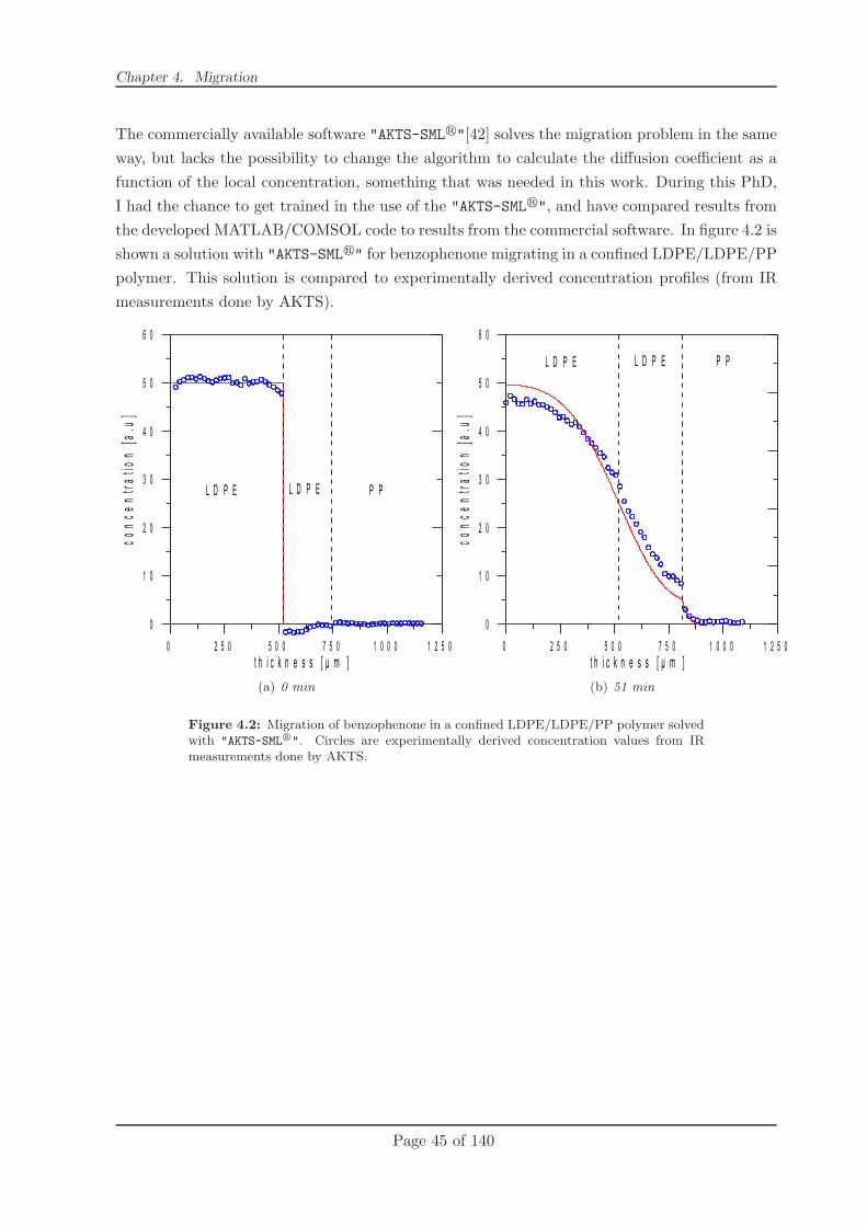
Chapter 4. Migration
The commercially available software "AKTS-SMLr"[42] solves the migration problem in the same
way, but lacks the possibility to change the algorithm to calculate the diffusion coefficient as a
function of the local concentration, something that was needed in this work. During this PhD,
I had the chance to get trained in the use of the "AKTS-SMLr", and have compared results from
the developed MATLAB/COMSOL code to results from the commercial software. In figure 4.2 is
shown a solution with "AKTS-SMLr" for benzophenone migrating in a confined LDPE/LDPE/PP
polymer. This solution is compared to experimentally derived concentration profiles (from IR
measurements done by AKTS).
(a) 0 min (b) 51 min
Figure 4.2: Migration of benzophenone in a confined LDPE/LDPE/PP polymer solvedwith "AKTS-SML
r". Circles are experimentally derived concentration values from IR
measurements done by AKTS.
Page 45 of 140

Chapter 4. Migration 4.1. Modeling of migration in highly plasticised PVC
4.1 Modeling of migration in highly plasticised PVC
The migration of additives in most polymers can be modeled with good results by analyti-
cal models like eq. 4.1 for simple systems. For very complex systems a numerical solution
may be required of the Partial differential equations (PDEs) of the Ficks second law of diffu-
sion by the use of finite element method (FEM), either by specialised software for migration
(i.e."AKTS-SMLr"[42] or "FABES-MIGRATESTr EXP"[43]) or by more generalized tools like "COM-
SOL Multiphysicsr"[44]. These solutions work only because the migration of the additive has
very little or no influence on the system, i.e. the concentration change of the additive in the
polymer does not affect the physical or chemical structure of the polymer.
For highly plasticised PVC this is however not the case, when the migrant of interest is either
the plasticiser itself or a migrant that has a plasticising effect. For PVC the diffusion coefficient
of the migrant can change from around 10−7 cm2/s for fully plasticised PVC to around 10−16
cm2/s for unplasticised, rigid PVC. This means that in highly plasticised areas the migration will
be fast and in areas with little plasticiser the structure will be very crystalline and with slow
migration. For PVC to be highly plasticised and flexible it needs to contain a volume percent
of the plasticiser between 30-60%. Using analytical solution this problem has been directed in
the article: ”Modeling of the Migration of Glycerol Monoester Plasticizers in Highly Plasticized
Poly(vinyl chloride)”. In this article it is described how this problem can be modeled with some
success using the analytical solution (eq. 4.2 original derived by Kondyli et al.[40] for migration
into solvents under agitation. This article can be seen in appendix A.
As an extension of this work it was investigated if the numerical solution by the FEM method
could be used to allow the diffusion coefficient to be dependent on the local plasticiser concen-
tration. This work is shown in the section 3.3 ”Concentration dependent diffusion coefficient”.
4.1.1 Conclusion
Highly plasticised PVC is a very complex polymer to model the migration, especially when
the concentration of the plasticiser changes over time. Using either the specialiced analytical
solution (eq. 4.2) or the approach of concentration dependent diffusion coefficients with the
numerical solution by FEM can give good fit to experimental data. The problem however with
both of these solutions is that still some parameters have to be fitted to the experimental data,
making both approaches difficult to use if no experimental data exist.
Page 46 of 140

Chapter 4. Migration 4.2. Modeling of antistatic additive migration
4.2 Modeling of antistatic additive migration
4.2.1 The antistatic additive project
The purpose of the antistatic project was to investigate and obtain an improved understand-
ing of the mechanisms that make different commercial available antistatic polymer additives
produced by Danisco effective antistatic agents in mainly polypropylene, but also in polyethy-
lene and other polyolefines. All antistatic agents produced by Danisco are different variants
of glycerol monostearate (GMS), and more specifically these products are mainly composed by
monoglycerides (but also some di- and triglycerides) from palmitic and stearic acids (see figure
4.3).
Figure 4.3: The main components of glycerol monostearate (GMS) used as antistaticadditive. Mono, di- and triglycerides where the fatty acid profile is most commonly amixture of palmitic and stearic acids.
It is believed that the GMS molecules migrate to the surface of the polymer and together with
water from the air they aggregate resulting to a current conducting layer (see figure 4.4), which
prevents building up of an antistatic charge on the polymer. For some reason the GMS-based
antistatic additive does not perform equally well in different polymers, even when added in the
same amount to the polymers. It is believed that the migration rate of GMS in the polymer is
the main reason for this behavior, i.e. too fast or too slow migration of GMS to the surface will
counteract the antistatic mechanism.
Page 47 of 140

Chapter 4. Migration 4.2. Modeling of antistatic additive migration
Figure 4.4: The proposed mechanism of aggregation of the glycerol monostearate andwater on the surface of the polymer to produce the antistatic effect.
A new research project was therefore launched by Danisco in summer 2009, where Rasmus
Lundsgaard contributed with expertise on migration modeling of additives in polymers. New
migration experiments were conducted at Danisco, and the purpose of the work presented here
was to model these new migration data obtained using the previously developed migration model
(see section4). The modelling results of the migration data available could hopefully lead to a
better understanding of the transport of the antistatic additive from the bulk polymer to the
surface.
The experimental work at Danisco included 4 different types of experiments run over 60 days
on the same systems and at same sampling times. The test systems consisted of either low den-
sity polyethylene (LDPE) or polypropylene (PP), where problems were encountered only when
the curent antistatic additive was used for the PP polymer. The antistatics used were either
an already commercially successful antistatic additive (DIMODAN HP), or a newly developed
candidate (PGE 308). The PGE 308 is still under development at Dannisco, and for this reason
can no further details be given regarding the structure of PGE 308.
A short description of the 4 experiments that were conducted at Danisco are presented in table
4.1.
Page 48 of 140

Chapter 4. Migration 4.2. Modeling of antistatic additive migration
Table 4.1: The 4 simultaneous experiments conducted in the antistatic additive studyat Danisco and RISØ-DTU.
Experiment Description and conclusion
Static decay time: Measurement of antistatic performance.The general conclusion from this experiment was:
DIMODAN HP PGE 308
LDPE Good Very goodPP poor to none none
Contact angle measure-ment:
This experiment was conducted by measuring the contactangle for each sample with only two solutes. The surfacetension from these experiments were thereby presented as apolar and a dispersive part. The measured surface tensionvalues from all the experiments did not lead to some safeconclusion,
XPS: X-ray photo-electron spectroscopy, which was used to mea-sure the specific oxygen concentration in layers carved fromthe surface of the polymer. This measurement was also con-ducted by Rasmus Lundsgaard at RISØ-DTU (a nationallaboratory under DTU). These measurements where con-ducted together with master student Julien Danguillaumeas a special course[45]. Unfortunately the XPS equipmentat RISØ suffered from a lot of breakdowns in the 60 daystest period, so oxygen surface concentration values measuredwere strongly deviating. Results from this experiment areshown in appendix B
Migration: Measurement of the amount of additive migrated to the sur-face at the sampling time-points selected. This was done bydipping the polymer into iso-octane for a predefined time in-terval (10 sec.), and then measure the amount of additive inthe iso-octane. These data have been used for the modelingpresented here.
4.2.2 Modelling
Initially the migration to the surface of all the measured additives in the two polymers as either
a ratio of the total additive in the systems (Mt/M∞) or as final amount (in mmole) were plotted
(see figure 4.5 and 4.6.
Page 49 of 140

Chapter 4. Migration 4.2. Modeling of antistatic additive migration
0 10 20 30 40 50 60
0
0.1
0.2
0.3
0.4
0.5
0.6
Time in days
0.30% Dimodan HP0.15% C12 monoglycerol0.15% Diglycerol monoester0.15% Minor components0.30% C12 monoglycerol0.30% Diglycerol monoester0.30% Minor components
Mt/M
∞
(a) Ratio
0 10 20 30 40 50 60
0
0.2
0.4
0.6
0.8
1
1.2
1.4x 10
−3
Time in days
0.30% Dimodan HP0.15% C12 monoglycerol0.15% Diglycerol monoester0.15% Minor components0.15% All PGE 3080.30% C12 monoglycerol0.30% Diglycerol monoester0.30% Minor components0.30% All PGE 308
mm
ole
/dm
2
(b) mmole
Figure 4.5: The Migration in LDPE over time, plotted as ratio of the total additive inthe systems (Mt/M∞) or as final amount in mmole per area (mmol/dm2).
From the collective plot of all additives migration to the surface of LDPE as a ratio of the total
additive in the polymer (figure 4.5 (a)), the migration seem to go towards the same ratio regard-
less of total concentration in the system (0.15% or 0.30%). Especially for C12 monoglyceride
does the migration go towards almost identical final ratios, even though there is a factor two of
difference in concentration. This information points towards a partition function between bulk
and surface being the controlling part for the final migration to the surface. When plotting the
migration as the final amount migrated (figure 4.5 (b), this information is not clear.
0 10 20 30 40 50 60
0
0.02
0.04
0.06
0.08
0.1
0.12
0.14
0.16
0.18
0.2
Time in days
0.60% Dimodan HP0.60% C12 monoglycerol0.60% Diglycerol monoester0.60% Minor components
Mt/M
∞
(a) Ratio
0 10 20 30 40 50 60
0
0.2
0.4
0.6
0.8
1
x 10−3
Time in days
0.60% Dimodan HP0.60% C12 monoglycerol0.60% Diglycerol monoester0.60% Minor components
mm
ole
/dm
2
(b) mmole
Figure 4.6: The Migration in PP over time, plotted as ratio of the total additive in thesystems (Mt/M∞) or as final amount in mmole per area (mmol/dm2).
Comparing the migration plots for the two polymers, we can see that the PGE308 components
migrate more to the surface in LDPE than in PP (both as ratio and as total amount), whereas
Page 50 of 140

Chapter 4. Migration 4.2. Modeling of antistatic additive migration
Dimodan HP seems to migrate towards the same ratio in both polymers.
From the migration data from Danisco, an estimate of the diffusion coefficient of the antistatic
additive migration to the surface was calculated utilizing equation 3.1 as in the chapter on
diffusion coefficients (chapter 3). But as shown in figure 4.7, it seems that there was not enough
data points in the first part of the migration where the migration is expected to have close
to a linear relationship to the square root of time. Moreover, the measured migration for C12
monoglyceride in PGE 308 in PP seem to have a migration from the surface into the polymer
(see figure 4.7 (b)). This was discussed in the project group at Danisco and it was believed to
be due to statistical uncertainties in the experimental equipment as the concentrations of the
additive are very low.
0 2 4 6 8 10 12
x 105
0
0.05
0.1
0.15
0.2
0.25
0.3
0.35
0.4
D=9.6196e−014
4(t/π)0.5 / L
Mt /
M∞
(a) LDPE
0 2 4 6 8 10 12 14
x 105
0
0.01
0.02
0.03
0.04
0.05
0.06
0.07
0.08
0.09
D=3.3164e−015
4(t/π)0.5 / L
Mt /
M∞
(b) PP
Figure 4.7: Estimation of the diffusion coefficient of C12 monoglyceride in PGE 308LDPE or PP as a linear function of the square root of time (eq. 3.1).
The calculations of diffusion coefficient for the additives were done both using the first three
sampling times (blue points in figure 4.8) and using the first sampling time (red points in figure
4.8). Moreover, for comparison reasons, the semi-empirical model (eq. 3.28) by Piringer with
general polymer parameters for PP and LDPE[14] was also used. This is shown in figure 4.8 as
the solid line. As it can be seen there is a large difference between the experimentally derived
and the fully estimated diffusion coefficients, by approximately 5 orders of magnitude.
Page 51 of 140
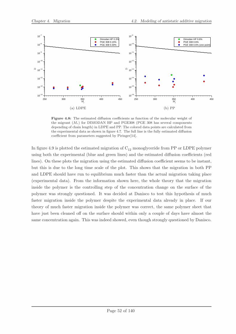
Chapter 4. Migration 4.2. Modeling of antistatic additive migration
250 300 350 400 450
10−14
10−13
10−12
10−11
10−10
10−9
10−8
10−7
Mr
D
Dimodan HP 0.3%PGE 308 0.15%PGE 308 0.30%
(a) LDPE
250 300 350 400 450
10−16
10−15
10−14
10−13
10−12
10−11
10−10
10−9
Mr
D
Dimodan HP 0.6%PGE 308 0.6%PGE 308 0.6% (one point)
(b) PP
Figure 4.8: The estimated diffusion coefficients as function of the molecular weight ofthe migrant (Mr) for DIMODAN HP and PGE308 (PGE 308 has several componentsdepending of chain length) in LDPE and PP. The colored data points are calculated fromthe experimental data as shown in figure 4.7. The full line is the fully estimated diffusioncoefficient from parameters suggested by Piringer[14].
In figure 4.9 is plotted the estimated migration of C12 monoglyceride from PP or LDPE polymer
using both the experimental (blue and green lines) and the estimated diffusion coefficients (red
lines). On these plots the migration using the estimated diffusion coefficient seems to be instant,
but this is due to the long time scale of the plot. This shows that the migration in both PP
and LDPE should have run to equilibrium much faster than the actual migration taking place
(experimental data). From the information shown here, the whole theory that the migration
inside the polymer is the controlling step of the concentration change on the surface of the
polymer was strongly questioned. It was decided at Danisco to test this hypothesis of much
faster migration inside the polymer despite the experimental data already in place. If our
theory of much faster migration inside the polymer was correct, the same polymer sheet that
have just been cleaned off on the surface should within only a couple of days have almost the
same concentration again. This was indeed showed, even though strongly questioned by Danisco.
Page 52 of 140

Chapter 4. Migration 4.2. Modeling of antistatic additive migration
0 10 20 30 40 50 60
0
0.05
0.1
0.15
0.2
0.25
0.3
0.35
0.4
0.45
0.5
Time in days
Data pointCrank with DestCrank with Dexp
Mt/M
∞
(a) LDPE
0 10 20 30 40 50 60
0
0.01
0.02
0.03
0.04
0.05
0.06
0.07
0.08
0.09
0.1
Time in days
Data pointCrank with DestCrank with DexpCrank with Dexp (one point)
Mt/M
∞
(b) PP
Figure 4.9: The modeled migration of the C12 monoglyceride in PGE 3008 to thesurface of either LDPE or PP over time. The red line is migration estimated using thediffusion coefficient fully estimated from parameters by Piringer[14], and green and bluelines are the migration with diffusion coefficients estimated from the first data points ofthe migration.
The new knowledge of the migration of the additive in the bulk polymer being faster than what
the experiments showed, lead to some new ideas on what was causing this migration to (and
from the) surface of the polymer. Diffusion is even faster at higher temperatures (e.g under the
extrusion), and the additive is mixed with the polymer before the final polymer film is extruded.
Thus, it is possible that already at the first sampling time, some equilibrium concentrations
of the additive in the bulk polymer and on the surface have been reached. This could also
explain how in some of the experiments there seems to be a migration back in to the polymer.
This is because the ”partition coefficient” between surface and bulk is different depending on
temperature. To obtain an estimate of this initial concentration of the additive on the surface,
it was chosen to use the first 2-3 data points from the migration and extrapolate back linearly
as a function of the square root of time as shown by the red line in figure 4.10.
Page 53 of 140

Chapter 4. Migration 4.2. Modeling of antistatic additive migration
0 2 4 6 8 10 12
x 105
0
0.05
0.1
0.15
0.2
0.25
0.3
0.35
0.4
4(t/π)0.5 / L
Mt /
M∞
(a) LDPE
0 2 4 6 8 10 12 14
x 105
0
0.01
0.02
0.03
0.04
0.05
0.06
0.07
0.08
0.09
4(t/π)0.5 / L
Mt /
M∞
(b) PP
Figure 4.10: Estimation of the initial concentration of C12 monoglyceride from PGE308 in LDPE and PP (red line). The blue line shows the correlation of the data to thesquare root of time using eq. 3.1.
It was then chosen to model the migration between the bulk polymer and the surface layer by
using the estimated diffusion coefficient for the bulk parameter. We model the surface layer as
an arbitrary specific layer of 0.05mm and fit the diffusion coefficient and partition coefficient
between the two layers against the migration data. The specific size of the surface layer is not
of paramount importance as the fitted partition coefficient (ratio of the amount of the migrant
in the two layers) is purely dependent of this size. In figure 4.11 is shown how the concentration
in LDPE will look in the two layers at start and end using this new approach.
0 0.01 0.02 0.03 0.04 0.05 0.06 0.070
5
10
15
Ct /
C0
time=0 days
(a) start
0 0.01 0.02 0.03 0.04 0.05 0.06 0.070
5
10
15
Ct /
C0
time=36 days
(b) end
Figure 4.11: Estimated migration of C12 monoglyceride in LDPE by the new approach.With the new approach there is already an additive concentration at the surface at thestarting point. The dotted red line at the plot of the end concentration illustrates thestarting concentration values.
In other words the only fitted parameters in this approach are the diffusion coefficient on the
surface layer (as it is believed now that the antistatic additive aggregates on the surface is the
Page 54 of 140
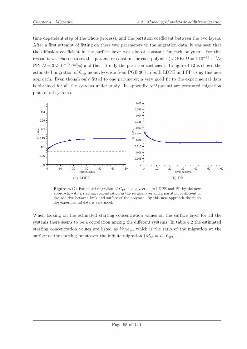
Chapter 4. Migration 4.2. Modeling of antistatic additive migration
time dependent step of the whole process), and the partition coefficient between the two layers.
After a first attempt of fitting on these two parameters to the migration data, it was seen that
the diffusion coefficient in the surface layer was almost constant for each polymer. For this
reason it was chosen to set this parameter constant for each polymer (LDPE: D = 1·10−14 cm2/s;
PP: D = 3.2·10−15 cm2/s) and then fit only the partition coefficient. In figure 4.12 is shown the
estimated migration of C12 monoglyceride from PGE 308 in both LDPE and PP using this new
approach. Even though only fitted to one parameter, a very good fit to the experimental data
is obtained for all the systems under study. In appendix refApp:anti are presented migration
plots of all systems.
0 10 20 30 40 50 600
0.05
0.1
0.15
0.2
0.25
0.3
Time in days
Mt/M
∞
(a) LDPE
0 10 20 30 40 50 600
0.005
0.01
0.015
0.02
0.025
0.03
0.035
0.04
0.045
0.05
Time in days
Mt/M
∞
(b) PP
Figure 4.12: Estimated migration of C12 monoglyceride in LDPE and PP by the newapproach, with a starting concentration in the surface layer and a partition coefficient ofthe additive between bulk and surface of the polymer. By this new approach the fit tothe experimental data is very good.
When looking on the estimated starting concentration values on the surface layer for all the
systems there seems to be a correlation among the different systems. In table 4.2 the estimated
starting concentration values are listed as M0/M∞, which is the ratio of the migration at the
surface at the starting point over the infinite migration (M∞ = L · Cp0).
Page 55 of 140

Chapter 4. Migration 4.2. Modeling of antistatic additive migration
Table 4.2: Estimated starting concentration values of the antistatic additive on thesurface layer as M0/M∞, calculated by regressing the three first data points as a functionof the square root of time (see figure 4.10). Mr is the molecular weight in g/mol.
LDPE PPMr
M0/M∞
M0/M∞
additive conc. 0.15% 0.30% 0.60%Dimodan
C16/C18 monoglycerid 344 0.094 0.042PGE 308
C12 monoglycerid 274 0.075 0.065 0.029Diglycerol monoester 348 0.040 0.039 0.013Total main 326 0.051 0.047 0.018Minor components 430 0.088 0.079 0.032Total all 342 0.056 0.051 0.020
It is now postulated that there is a linear relationship between the concentration of the additive
in the polymer and the estimated concentration of the additive at the surface at the starting
point. The average factor for the change from 0.15% to 0.30% of the PGE 308 components in
LDPE is -0.0058. Using this average concentration factor, all the values of PGE 308 in LDPE
can be recalculated as if the additive concentration was 0.60%. These new recalculated surface
start concentration values from LDPE can then be used to find an average polymer change
factor for the change between LDPE and PP. The average polymer change factor was found
to be 0.49. The two average change parameters make it possible to recalculate the surface
start concentration values both with change of additive concentration and between LDPE and
PP polymers. In table 4.3 the three sets of surface start concentration values are given when
recalculated to be from LDPE for an additive concentration of 0.60%. As it can be seen it
seems that this initially postulated linear correlation in both concentration change and change
in polymer is confirmed.
From these three sets of recalculated surface start concentration values obtained as if there was
only one system, a new overall average surface start concentration value set can be derived (see
table 4.3).
Table 4.3: Surface start concentrations from the three data sets (see table 4.2, recalcu-lated using the two average change parameters (polymer change parameter: 0.49; additiveconcentration change parameter: -0.0058/(0.15%)). The three sets are recalculated to beas data from LDPE with a additive concentration of 0.60%.M0/M∞ PP LDPE LDPE
0.60% 0.15% 0.30% AverageDimodan
C16/C18 monoglycerid 0.086 0.082 0.084PGE 308
C12 monoglycerid 0.059 0.058 0.053 0.057Diglycerol monoester 0.027 0.023 0.027 0.026Total main 0.037 0.034 0.035 0.035Minor components 0.065 0.071 0.067 0.068Total all 0.041 0.039 0.039 0.040
Using this new overall average surface concentration data set and the polymer and concentration
Page 56 of 140

Chapter 4. Migration 4.2. Modeling of antistatic additive migration
change factors, an estimation for all systems can be accomplished. This is shown in table 4.4.
A very good correlation to all the ”experimental” data is obtained.
Table 4.4: Estimated surface start concentration for all possible systems in the LDPEpolymer. Estimations are done using the new average surface concentration set (seetable 4.3) and the two average change parameters. The estimated surface concentrationsresult in very accurate correlation of the two sets of experimental data derived surfaceconcentrations.
M0/M∞ 0.15% 0.30% 0.45% 0.60%Est Exp Est Exp Est Est Exp
LDPEDimodan
C16/C18 monoglycerid 0.101 0.096 0.094 0.090 0.084PGE 308
C12 monoglycerid 0.074 0.075 0.068 0.065 0.063 0.057Diglycerol monoester 0.043 0.040 0.037 0.039 0.031 0.026Total main 0.053 0.051 0.047 0.047 0.041 0.035Minor components 0.085 0.088 0.079 0.079 0.074 0.068Total all 0.057 0.056 0.051 0.051 0.045 0.040
PPDimodan
C16/C18 monoglycerid 0.059 0.053 0.047 0.041 0.042PGE 308
C12 monoglycerid 0.045 0.039 0.034 0.028 0.029Diglycerol monoester 0.030 0.024 0.018 0.013 0.013Total main 0.035 0.029 0.023 0.017 0.018Minor components 0.051 0.045 0.039 0.033 0.032Total all 0.037 0.031 0.025 0.019 0.020
The same methodology was followed using the obtained partition coefficients, but the correlation
did not prove to be satisfactory. In table 4.5 the fitted partition coefficients are listed for all the
systems.
Table 4.5: Fitted partition coefficients (Kp) for all tested additives between bulk andsurface layers (0.05mm) in both LDPE and PP. No direct correlation was found betweenthe three data sets of fitted partition coefficients.
LDPE PPMr Kp Kp
additive conc. 0.15% 0.30% 0.60%Dimodan
C16/C18 monoglycerid 344 0.12 0.02PGE 308
C12 monoglycerid 274 0.15 0.18 1.50Diglycerol monoester 348 0.12 0.17 2.50Total main 326 0.13 0.17 2.15Minor components 430 0.06 0.09 1.20Total all 342 0.11 0.15 1.90
In appendix C is shown the migration plots of all the systems using the fitted partition coefficients
listed in table 4.5 and the estimated surface start concentrations from table 4.4.
Page 57 of 140

Chapter 4. Migration 4.2. Modeling of antistatic additive migration
4.2.3 Conclusion
The main conclusions from this modeling work on antistatic additive migration in LDPE and PP
is that the migration in the polymer bulk is not the time limiting step of the migration process of
the antistatic agent to the surface. This is a very important conclusion as the opposite has been
a strong belief of Danisco for more than 10 years. The next step steaming from this conclusion is
to discover the controlling step which defines how fast the additive migrates to the surface. The
second main conclusion from this modeling work is that it is possible to obtain a very good fit to
the migration data with the proposed model. The new model stimulates that the system has a
thin surface layer and specific diffusion coefficients for both bulk polymer and surface layer. The
partition coefficient of the additive between the bulk and the surface is temperature dependent.
Moreover is the migration in the polymer mush faster at higher temperature, which means the
migration to the surface layer started to happen already in the extrusion process of the polymer
film.
From the model it can be concluded that there is a strong correlation between the systems
regarding the additive surface concentration right after the extrusion proces. This correlation
does not seem to hold for the final surface concentration. This could point towards that over
time some sort of structural change of the additive molecules happens on the surface that makes
it more or less favorable for them to be there. To understand what happens on the surface of
the polymer with the antistatic additive molecules, which turns out to be the controlling part
of the migration to the surface, a correlation has to be found between the partition coefficient
and some other parameter for the additive (i.e. molar volume or polarity).
Page 58 of 140

Chapter 5Modeling partition coefficients in
polymer/solvent systems by molecular
dynamics
Accurate partition coefficient data of migrants between a polymer and a solvent are of paramount
importance for estimating the migration of the migrant over time, especially for estimating the
concentration of the migrant at infinite time in the two solvents (i.e. the polymer and the food
simulant).
Most predictive models for partition coefficients in polymer/solvent or polymer/polymer systems
are based on thermodynamic models for the estimation of the activity coefficient. A comparison
study by Piringer and Baner in 2008[14] for up to 13 organic substances in different polymers
and solvent systems showed an average absolute error ratio for the estimated partition coefficient
with these activity coefficient models around 5-10 (best case scenario), and sometimes up to
10.000. Many of the thermodynamic models in that study predict a partition coefficient for
the polyethylene (PE) / ethanol systems larger than unity for one or more compounds (higher
affinity for PE than for ethanol), even though the experimental partition coefficients for this
system are below unity (higher affinity for ethanol than for PE). In a recent article by Gillet
et al.[46], another approach was proposed based on a generalized Flory-Huggins model together
with Metropolis Monte Carlo (MC) calculations for the Flory-Huggins interaction parameters.
This approach aims towards keeping the flexibility of the Flory-Huggins model for calculations
at the macroscopic scale, while obtaining only the system-specific interaction parameters from
the fairly cheap (for polymeric systems) computational MC calculations at the atomistic scale.
A more direct approach would include the performance of all calculations at the atomistic
scale using Molecular Dynamics (MD) simulations to calculate the free energy of solvation by
thermodynamic integration[47]. From this free energy of solvation of the solute into each of the
two solvents (∆solvAG and ∆solvBG in eq. 5.1), the partition coefficient of the solute between
the two solvents can be calculated[48, 49].
Page 59 of 140

Chapter 5. Modeling partition coefficients 5.1. Molecular Dynamics
log KsolvA/solvB =∆solvBG − ∆solvAG
2.303RT(5.1)
In the current work this proposed methodology was firstly used for the calculation of partition
coefficients of additives into squalane (to mimic low-density polyethylene (LDPE)) and food
simulant A (distilled water) or food simulant C (10% ethanol, 50% ethanol). These specific
systems were chosen because good experimental data exist for the partition coefficients in all
of them with cis-3-hexenol and decane[14]. The choice of these two specific solutes is based on
their fairly simple structure and the fact that one is hydrophobic and the other hydrophilic.
The calculations and the methodology used for the systems on squalane and ethanol/water is
presented in the article ”Partition coefficients of organic molecules in squalane and water/ethanol
mixtures by Molecular Dynamics Simulations”submitted to the Journal of Fluid Phase Equilibria
(FPE) for review. This article as it is submitted is presented in the section 5.2 ”Partition
coefficients of organic molecules in squalane and water/ethanol mixtures by Molecular Dynamics
Simulations”.
5.1 Molecular Dynamics
Molecular Dynamics (MD) is a time-dependent algorithm used in Molecular Simulations where
molecules are represented as specific centers in a virtualbox and all the inter atomic interactions
are modeled by bonded and non-bonded interaction functions. The time development of the
system happens by movement of the centers in the box according to the Newton’s laws of
motion. Depending on the choice of scale of the force field the centers in this work represent all
atoms of the molecule (All Atoms force field, like OPLS-AA[7] and CHARMM27[5, 50]). The
molecules can also be represented with most hydrogen atoms implicit together with the nearest
center, called United Atom force fields (UA). This means for instance that CH3 or CH2 are
calculated as one center, in this work the TraPPE force field).
Page 60 of 140

Chapter 5. Modeling partition coefficients 5.1. Molecular Dynamics
Figure 5.1: Bonded and nonbonded interactions in molecular dynamics[51].
The molecular dynamics calculations in this work are performed using the open-source code
GROMACS (version 4)[6]. In GROMACS the non-bonded and bonded interactions (see figure
5.1) are modeled by the following equations:
Lennard-Jones interactions are calculated between all non-bonded centres and bonded centres
more than 2 bonds away. Most force fields use a special scaling factor (S) for the interaction
specifically between atoms with three bonds distance (1-4 interaction). For TraPPE SLJ=0, for
OPLS-AA SLJ=0.5 and for the CHARMM27 force field the 1-4 LJ interactions are predefined
in the force field.
ELJ(rij) = 4ǫij
(
(
σij
rij
)12
−(
σij
rij
)6)
SLJ (5.2)
where rij is the distance between center i and j, ǫij is the depth of the LJ potential well and σij
is the finite distance of the LJ potential.
Coulomb interactions are calculated in the same way, also often with a special scaling fac-
tor (SC) used for the 1-4 interactions. For TraPPE SC=0.5, for OPLS-AA SC=0.5 and for
CHARMM27 SC=1.
EC(rij) =qiqj
4πǫ0ǫrrijSC (5.3)
where q is the atomic charge and ǫ0 is the dielectric constant in vacuum and ǫr is the dielectric
constant of the medium.
Bond stretching between bonded molecules are modelled by a simple harmonic potential:
Eb(rij) =1
2kb
ij (rij − bij)2 (5.4)
Page 61 of 140

Chapter 5. Modeling partition coefficients 5.1. Molecular Dynamics
where kbij is the bond force constant and bij is the optimal bond length.
Angle bending between 1-3 bonded molecules are also modelled by a harmonic potential:
Ea(θijk) =1
2kθ
ijk
(
θijk − θ0ijk
)2(5.5)
where kθijk is the angle force constant, θijk is the angle between center i,j and k and θ0
ijk is the
optimal angle.
Torsional angle bending (1-4 angle) is modelled by a Ryckaert-Bellemans (RB) function:
Erb(φijkl) =5∑
n=0
Cn (cos(φijkl))n (5.6)
where φijkl is the 1-4 torsional angle (there are different definitions for when the torsional angle
is 0, it can be either at the trans or the cis position. GROMACS follows the ’polymer conven-
tion’ of φtrans = 0), Cn are the Ryckaert-Bellemans parameters specific for each set of center ijkl.
Page 62 of 140

Chapter 5. Modeling partition coefficients 5.2. Partition coefficients article
5.2 Partition coefficients of organic molecules in squalane and
water/ethanol mixtures by Molecular Dynamics Simulations
Rasmus Lundsgaard1, Georgios M. Kontogeorgis1 & Ioannis G. Economou2
(1) Center for Energy Resources Engineering (CERE), Department of Chemical and Biochemical
Engineering, Technical University of Denmark, Kgs. Lyngby DK-2800, Denmark;
(2) The Petroleum Institute, Department of Chemical Engineering, Abu Dhabi, PO Box 2533, United
Arab Emirates
(Submitted to Journal of Fluid Phase Equilibria, September 2010)
5.2.1 Abstract
Accurate partition coefficient data of migrants between a polymer and a solvent are of paramount
importance for estimating the migration of the migrant over time, including the concentration
of the migrant at infinite time in the two solvents. In this article it is shown how this partition
coefficient can be estimated for both a small hydrophilic and a hydrophobic organic molecules
between squalane (used here to mimic low density poly ethylene) and water/ethanol solutes
using thermodynamic integration to calculate the free energy of solvation. Molecular dynamics
simulations are performed, using the GROMACS software, by slowly decoupling of firstly the
electrostatic and then the Lennard-Jones interactions between molecules in the simulation box.
These calculations depend very much on the choice of force field. Two force fields have been
tested in this work, the TraPPE-UA (united-atom) and the OPLS-AA (all-atom). The compu-
tational cheaper TraPPE-UA force field showed to be more accurate over the whole range of
systems compared to the OPLS-AA force field. Moreover, some of the calculations were done
with five different water models to investigate the influence of the specific water model on the
calculations. It was found that the combination of the TraPPE-UA force field and the TIP4p
water model gave the best results. Based on the methodology proposed in this article, it is pos-
sible to obtain good partition coefficients only knowing the chemical structure of the molecules
in the system.
5.2.2 Introduction
In the later years it has been approved by EU to estimate migration of additives from a mono-
layer polymer into a solvent utilizing a generally recognized migration model[16] or even from
multilayer polymer systems into a solvent utilizing finite element method (FEM). These models
are only as good as the parameters used, i.e. diffusion coefficients and partition coefficients. The
model proposed by Piringer[14] made for safe over estimation of diffusion coefficients has been
approved by EU, when no or only very little data exist. By the term “safe over estimation” is
meant an estimation model that is the worst case scenario estimation for at least 95% of the
data. On the other hand, for partition coefficients, there is currently no approved consistent
model. For simplification and unification of the experimental work and/or calculations that has
to be done in order to get a product approved by the legislation, four food simulants have been
Page 63 of 140

Chapter 5. Modeling partition coefficients 5.2. Partition coefficients article
chosen by the European Commision[52]:
A Distilled water
B 3% Acetic Acid (weight/volume)
C 10% Ethanol (volume/volume)
D Olive oil or Sunflower oil (in some cases Iso-octane)
In the specific case of milk and similar products, it is suggested to use 50% ethanol as the food
simulant.
Most models for prediction of partition coefficients in polymer/solvent or polymer/polymer sys-
tems are based on thermodynamic models for the estimation of the activity coefficient. A
comparison study by Piringer and Baner in 2008[14] for up to 13 organic substances in different
polymers and solvent systems showed an average absolute ratio for the estimated partition co-
efficient with these activity coefficient models for the best around 5-10, and some up to 10000.
Many of the thermodynamic models predict a partition coefficient for the polyethylene (PE)
/ ethanol systems larger than unity for one or more compounds (higher affinity for PE than
for ethanol), even though that the experimental partition coefficients for this system are below
unity (higher affinity for ethanol than for PE).
In a recent article by Gillet et al.[46], another approach was proposed based on a generalized
Flory-Huggins model together with Metropolis Monte Carlo (MC) calculations for the Flory-
Huggins interaction parameters. This approach is aimed towards keeping the flexibility of the
Flory-Huggins model for calculations at the macroscopic scale, while obtaining only the system
specific interaction parameters from the fairly cheap (for polymeric systems) computational MC
calculations at the atomistic scale.
A more direct approach is doing all calculations at the atomistic scale using Molecular Dynamics
(MD) simulations to calculate the free energy of solvation by thermodynamic integration[47].
From this free energy of solvation of the solute into each of the two solvents, the partition co-
efficient of the solute between the two solvents can be calculated as shown by Best et al.[48].
In their article, this proposed methodology was used for calculation of partition coefficients of
additives into squalane (to mimic low-density polyethylene (LDPE)) and food simulant A (dis-
tilled water) or food simulant C (10% ethanol, 50% ethanol).
The purpose of this work is to investigate the proposed methodology to obtain good partition
coefficients from only the knowledge of the chemical structure of the molecules involved. The
article is organized as follows: Part 5.2.3 refers to the theory behind the calculation of the free
energy of solvation and how to get the partition coefficient from it; in Part 5.2.4, the force fields
for the various molecules are presented and their implementation in the GROMACS software;
Page 64 of 140

Chapter 5. Modeling partition coefficients 5.2. Partition coefficients article
Part 5.2.5 refers to Computational details, Part 5.2.6 is devoted to Results and discussion and
in Part 5.2.7 Conclusions are drawn.
5.2.3 Partition coefficients from thermodynamic integration
It have been shown by Essex et al.[49] that from the free energy of solvation in solvent A and B
(∆solvAG and ∆solvBG in equation 1) it is possible to estimate the partition coefficient between
the two solvents:
log KsolvA/solvB =∆solvBG − ∆solvAG
2.303RT(5.7)
Calculating the free energy of solvation by thermodynamic integration from molecular dynamics
is, however, not completely straight forward, as slowly stepwise elimination of all the solvent
molecules is not possible. Instead, the thermodynamic cycle (figure 5.2) can be used to calculate
this change, by calculating the other steps.
Figure 5.2: Thermodynamic cycle where ∆pureG is the free energy associated with thechange from a solute molecule with full Lennard-Jones (LJ) and Coulombic interactions(both inter, and intra molecular) into no interactions (a dummy molecule), ∆vacG is thefree energy associated with the same process in vacuum (only intra molecular interac-tions), and finally ∆dummyG can be seen as the hypothetical free energy of solvationdummy molecules.
Page 65 of 140

Chapter 5. Modeling partition coefficients 5.2. Partition coefficients article
Calculations can be done knowing:
1 Decoubling of all interactions from solute in solvent gives ∆pureG
2 Decoubling of all interactions from solute in vacuum gives ∆vacG
3 The change in free energy from a dummy molecule in solvent into vaccum is zero
A dummy molecule is a molecule that has no Lennard-Jones (LJ) and Coloumbic interactions
(either intra- and intermolecular), but there is still the intramolecular bonded interaction. The
intramolecular bonded interactions are, however, the same both in solute and vacuum, hence
∆dummyG is equal to zero and the equation for the thermodynamic cycle can be written as:
∆solvG = ∆vacG − ∆pureG − ∆dummyG = ∆vacG − ∆pureG (5.8)
As inter- and intramolecular LJ and Coulombic interactions in standard simulation algorithms
are indistinguishable from each other when doing the slowly decoupling of interactions from the
solute (going from box 1 to 2 in figure 5.2), the separate calculation in vacuum is necessary to
compensate for changes in solute-solute intramolecular interactions that take place for the solute
in the solvent (box 3 to 4 in figure 5.2). By separating the energy into individual components
this becomes a bit clearer. The initial state of the ∆pureG calculation (box 1 in figure 5.2) can
in this way be written as:
Gλ=0pure = GB
aa + Gintraaa + GB
bb + Gintrabb + Ginter
bb + Ginterab (5.9)
Where index a denotes the solute molecule and index b denotes the solvent molecule. GB
represents the free energy from intramolecular bonded interactions (bond stretching, bond angle
bending and dihedral torsion). λ is a decoupling parameter used for the slowly decoupling of
all LJ and Coulombic interactions of the solute molecule, when λ = 0 there is no decoupling –
ie full LJ and Coulombic interactions. As there only is one solute molecule in the box the inter
molecular distance between two solute molecule centers will always be greater than half the box
length. For this reason the term can be neglected.
In the final state for the ∆pureG calculation, the LJ and Coulombic interactions between the
solute and the solvent are turned off (λ = 1), by changing their LJ parameters and point charges
to zero. This will however also turn off the intramolecular LJ and Coulombic interactions of the
solute, as these are indistinguishable (box 2 in figure 5.2).
Gλ=1pure = GB
aa + GBbb + Gintra
bb + Ginterbb (5.10)
By combining equations 5.9 and 5.10, ∆pureG can be calculated as:
Page 66 of 140

Chapter 5. Modeling partition coefficients 5.2. Partition coefficients article
Gpure = Gλ=1pure − Gλ=0
pure = −Gintraaa − Ginter
ab (5.11)
For ∆vacG it is a bit simpler:
Gλ=0vac = GB
aa + Gintraaa (5.12)
Gλ=1vac = GB
aa (5.13)
Gvac = Gλ=1vac − Gλ=0
vac = −Gintraaa (5.14)
Finally, by substituting equations 5.11 and 5.14 into 5.8:
∆solvG = ∆vacG − ∆pureG = Ginterab (5.15)
Thus, it is clear that in order to obtain a correct free energy of solvation, independent simulations
both in vacuum and in solvent have to be done. For each case, the free energy can be estimated
using different methods, such as free energy perturbation, thermodynamic integration or the
slow-growth method[53]. For relatively large solutes, thermodynamic perturbation is impractical
due to the difficulty in successfully inserting an entire solute molecule into an equilibrated solvent
box. Slow-growth methods suffer from hysteresis problems and may introduce uncontrolled
systematic errors in the calculations[54]. So for this reason thermodynamic integration has been
chosen as the way of estimating the free energy.
The initial state and the final state has two different Hamiltonian functions (H0(x, px) and
H1(x, px)), where x and p are the positions and the momenta of all the atoms respectively.
By parameterizing the Hamiltonian (Hλ(x, px)) with the coupling parameter λ such that when
λ = 0, Hλ = H0 and when λ = 1, Hλ = H1, then the free energy becomes also a function of λ:
dA
dλ=
⟨
∂Hλ (x, px)
∂λ
⟩
λ
⇒ (5.16)
∆A =
∫ 1
0
⟨
∂Hλ (x, px)
∂λ
⟩
λ
dλ = ∆G
In this approach it is assumed that Hλ interpolates smoothly between the two Hamiltonian
functions. The calculations are done in practice by considering a set of independent and discrete
λ values between 0 and 1. For each λ value, the derivatives of the free energy with respect to
Page 67 of 140

Chapter 5. Modeling partition coefficients 5.2. Partition coefficients article
λ are evaluated and averaged. Integrating along the smoothed interpolated function between
the two states gives the final free energy difference (eq. 5.17). This means that the overall free
energy of solvation can be calculated by:
∆solvG =
∫ 1
0
⟨
∂Hλ (x, px)
∂λ
⟩vac
λ
dλ −∫ 1
0
⟨
∂Hλ (x, px)
∂λ
⟩pure
λ
dλ (5.17)
Splitting this approach up into two steps, firstly decoupling of the Coulombic interactions and
then decoupling of the Lennard-Jones interactions will give a more accurate result and a more
well-behaved function between the two states, as shown by Shirts et al.[55].
5.2.4 Force fields
Initially, three different force fields were chosen for this work, the “Transferable Potentials for
Phase Equilibria” united-atom force field (TraPPE-UA)[8], the “Groningen Molecular Simula-
tion” force field (GROMOS, united atom)[56] and the “Optimized Potentials for Liquid Simula-
tions” force field (OPLS-AA, all atom)[7]. For the GROMOS force field the latest parameter set
53A6 was chosen, as this parameter set specifically is adjusted to reproduce the free enthalpies of
hydration in Simple Point Charge (SPC) water[57]. The problem with this force field showed to
be the inconsistency in choice of the atomic charges in organic molecules, because this force field
is parameterized towards biomolecular systems, which means that the atomic charges should be
decided based on analogy to the functional groups in amino acids. As the software PRODRG[58]
already was used to make coordinate files of the molecules, the ability of the software to estimate
the topology information for GROMOS force fields was also tested. The PRODRG software can
estimate atomic charges in the molecule as either reduced or full charges, both were tested. No
consistent way of setting these atomic charges was found for the first simple organic molecules
used in this work that could give good consistent free enthalpies of hydration. For this reason
this force field was not further considered.
In Table 5.1 all the recalculated non-bonded parameters of the TraPPE-UA and the OPLS-AA
force fields are shown in the form that they have been used in the GROMACS software, i.e. σ in
nm and ǫ in kJ/mol, where ǫ in the original literature of the force fields[7, 8, 59–61] are given as
either kcal/mol or K. All the bonded interactions (bond length, bond angles and dihedral angles)
are also recalculated from the parameters as in the original articles to parameters used in the
functions for bonding energies in Gromacs. It should be noted that there is a small difference
in the calculations of the LJ and Coulomb 1-4 interactions (LJ and Coulombic intramolecular
interactions between atoms separated by exactly 3 bonds) with the two force fields. For the
TraPPE-UA force field the Coloumbic 1-4 interaction are scaled by a factor of 0.5, and the 1-4
LJ interactions do not exist (scaled by a factor of 0). For the OPLS-AA force field both the
Coloumbic and LJ 1-4 interaction are scaled by a factor of 0.5.
Page 68 of 140

Chapter 5. Modeling partition coefficients 5.2. Partition coefficients article
Table 5.1: Non bonded parameters for TraPPE-UA and OPLS-AA force fields as im-plemented in the GROMACS software in this work.
Force field Atom/group qi σii ǫii
[e] [nm] [kJ/mol]
TraPPE-UA[8] CH3, (RCH3) 0.000 0.375 0.8148[8] CH2, (R2CH2) 0.000 0.395 0.3825[59] CH, (R3CH) 0.000 0.468 0.0831[60] CH−−, (RCH−−R) 0.000 0.373 0.3908[61] CH2, (RCH2OH) 0.265 0.395 0.3825[61] O, (ROH) -0.700 0.302 0.7732[61] H, (ROH) 0.435 0.000 0.0000
OPLS-AA[7] C, (RCH3) -0.180 0.350 0.276144[7] C, (RCH2R) -0.120 0.350 0.276144[7] H, (CHx) 0.060 0.250 0.125520[7] C, (RCH−−) -0.115 0.355 0.317984[7] H, (HC−−) 0.115 0.242 0.125520[7] C, (RCH2OH) 0.145 0.350 0.276144[7] O, (ROH) -0.683 0.312 0.711280[7] H, (ROH) 0.418 0.000 0.000000
The LJ interactions between unlike atoms are calculated through the combining rule of the
LJ interaction parameters between like atoms (ǫii and σii). For the OPLS-AA force field, a
geometric mean rule is used for both the σ and ǫ:
σij =√
σiiσjj, ǫij =√
ǫiiǫjj (5.18)
For the TraPPE-UA force field, on the other hand, the more common Lorentz-Berthelot com-
bining rule is used (equation 5.19). This led to the problem of how to calculate LJ interactions
when doing simulations with a combination of the two force fields in the same box. It was chosen
for simplification to use the Lorentz-Berthelot combining rule between all unlike atoms in the
box, irrespective of which force field was used for the specific atoms.
σij =1
2(σii + σjj) , ǫij =
√ǫiiǫjj (5.19)
Figure 5.3: 3 site and 4 site water models. In 4 site models, a dummy atom (D) exhibitsCoulombic interactions and oxygen atom exhibits Lennard-Jones interactions only.
Page 69 of 140

Chapter 5. Modeling partition coefficients 5.2. Partition coefficients article
Initially, in this work the SPC/E water model[57] was chosen. This is a three site water model and
for this reason it is fairly cheap computationally. The partition coefficients calculated between
squalane and ethanol-water systems were in general over predicted, as was seen for the system
squalane/pure water. For this reason, additional calculations were made with the SPC, SPC/E,
TIP4p[62], TIP4pEw[63] and TIP4p2005[64] water models. The TIP4p type water models are
four site models with a dummy atom that exhibits only Coloumbic interactions (the oxygen atom
has no Coloumbic interactions, see figure 5.3), whereas the SPC and SPC/E both are three site
models. The parameters of all 5 water models are shown in Table 5.2 with parameter values as
implemented in GROMACS.
Table 5.2: The different parameters for the water models used in this work. All pa-rameters are recalculated as they are implemented in the GROMACS software and notin the way they are listed in the original literature.
SPC SPC/E TIP4p TIP4pEw TIP4p2005[57] [57] [62] [63] [64]
σii [nm] 0.3116 0.3116 0.3154 0.316435 0.31589ǫii [kJ/mol] 0.6485 0.6485 0.6487 0.6810 0.7749
qO / qO [e] -0.8200 -0.8476 -1.0400 -1.04844 -1.1128qH [e] 0.4100 0.4238 0.5200 0.52422 0.5564
rOH [nm] 0.1 0.1 0.09572 0.09572 0.09572rHH [nm] 0.16330 0.16330 0.15139 0.15139 0.15139αD 0.1280 0.10668 0.13194
rD = rO + αD(rH1 − rO) + αD(rH2 − rO) (5.20)
The position of the dummy atom (rD) can be calculated as a function of the positions of the
hydrogens (rH1 and rH2) and the oxygen (rO) atoms as shown in equation 5.20. The αD number
is a ratio of the oxygen-dummy distance (|OD|) over half the distance from the oxygen to the
baseline between the two hydrogen atoms.
αD =|OD|
2 cos |∠DOH| · |OH| (5.21)
5.2.5 Computational details
All the calculations have been done using the Gromacs 4.0.5 software[6] on either an Ubuntu
Linux workstation (Intel Quad-core 3.00GHz) or on an Apple OSX workstation (Intel Xeon
Quad-core 2.80 Ghz). As Gromacs is developed towards MD simulations of biomolecules, the
binaries are by default compiled with single precision. In this work all calculations have been
done with binaries compiled with double precision. The MD calculations were done using the
approach of Mobley et al.[65] with the Langevin (stochastic) dynamics integrator to also control
Page 70 of 140

Chapter 5. Modeling partition coefficients 5.2. Partition coefficients article
the temperature[66]. This was done with a frictional constant of 1 ps−1, a reference temperature
of 298K and a overall step size of 2fs. A cut-off radii of 1 nm for the short-range neighbor list
was used, while electrostatic interactions were calculated using Reaction-Field[67] method with
a 1 nm cut-off radii and LJ interactions with a switched cut-off 0.8 - 0.9 nm. In the NPT runs
the Berendsen barostat[68] with a time constant of 0.5 ps and an isothermal compressibility of
4.5·10−5 bar−1 was used to enforce a proper pressure coupling. The box size was scaled at every
time step, and the reference pressure was set to 1 bar. The soft-core expression[69] has shown
to eliminate singularities and numerical instabilities in free energy calculation, especially at the
end points of the transformation between states (λ close to 0 or 1)[53]. For this reason the soft-
core expression was used for the secondary step (the turn off of LJ interactions). The soft-core
parameter was set to 0.5, the power for λ in the soft-core function was 1 and the soft-core σ
value was 0.3 nm.
For each simulation cycle the procedure was as follows:
1 Energy minimization using two minimization algorithms
a L-BFGS algorithm of Nocedal (5000 steps)
b Steepest descent minimization (500 steps)
2 Equilibration run with constant volume (10 ps, NVT)
3 Equilibration run with constant pressure using the Berendsen barostat (100 ps, NPT)
4 Production run the (5000 ps, NVT)
This cycle on this type of hardware takes approximately 50 min. which means that calculation
of a partition coefficient with the methodology proposed in this article takes approximately 20
× 50 min = 17 hours. When this project started only Gromacs version 3.3 was available, but
with the update to version 4.0.x, an increase in speed of up to 20% was seen. Moreover, the
choice of parallelization software had an influence on the speed when running on more than one
core (in this work the ”Open MPI” software has been used).
The number of solvent molecules in the boxes where:Squalane : 31
Ethanol/Water
0% (pure water) : 0 / 890
9% (mol./mol.) : 65 / 667 ≈20% (vol./vol.)
20% (mol./mol.) : 130 / 494 ≈40% (vol./vol.)
61% (mol./mol.) : 260 / 166 ≈80% (vol./vol.)
100% (pure ethanol) : 272 / 0
Page 71 of 140

Chapter 5. Modeling partition coefficients 5.2. Partition coefficients article
5.2.6 Results and discussion
Analysis of the stepwise λ decoupling methodology
As explained earlier, the enthalpy of solvation can be calculated by thermodynamic integration
over the stepwise decoupling of solvent-solute interactions. In this work the approach of Shirts
et al.[55] has been chosen which essentially means firstly a slowly decoupling of Coloumbic
interactions as a function of λ (see figure 5.4).
0 0.1 0.2 0.3 0.4 0.5 0.6 0.7 0.8 0.9 1−20
0
20
40
60
80
100
λ
∂ H
/ ∂
λ
OPLS−AA (SPCE)TraPPE (SPCE)OPLS−AA (Ethanol)TraPPE (Ethanol)
(a)
0 0.1 0.2 0.3 0.4 0.5 0.6 0.7 0.8 0.9 1−90
−80
−70
−60
−50
−40
−30
−20
−10
0
λ
∂ H
/ ∂
λ
OPLS−AA (SPCE)TraPPE (SPCE)OPLS−AA (Ethanol)TraPPE (Ethanol)
(b)
Figure 5.4: Decoupling of Coulombic interactions between cis-3-hexenol and SPC/Ewater or ethanol (λ = 0 is full interaction and λ = 1 is no interaction). Differencesare seen between the decoupling functions with the two force fields, due to one beingall-atom and the other united-atom (a). Circles are simulations in solvent, and crossesare in vacuum. The decoupling of solute-solvent interactions (difference between vacuumand solvent simulations) shows very similar decoupling function for the two force fields(b).
When λ = 0, full Coloumbic interactions are exhibited by the solute molecules, while for λ = 1
Coloumbic interactions are zero. As the decoupling of the Coloumbic interactions has shown to
be a very smooth function and the calculations of the electrostatics is the most time consuming
part of MD simulations, it was chosen to perform calculations for the following λ values {0.0; 0.1;
0.2; 0.4; 0.5; 0.6; 0.8; 0.9; 1.0}. In figure 5.4, the decoupling of Coloumbic interactions are shown
for cis-3-hexenol in either SPC/E water or ethanol with both OPLS-AA and the TraPPE-UA
force fields. In Figure 5.4 (a), are shown the decoupling in both the solvent and in vacuum.
As described earlier (equation 5.15), the difference between these two simulations is exactly the
decoupling of intermolecular Coloumbic interactions between solvent and solute, which can be
seen in Figure 5.4 (b).
The decoupling of LJ interactions is made after the decoupling of the Coloumbic interactions,
which means that the solute molecule in this step has no atomic charges. This means that the
calculations are computational less expensive and for this reason the calculations were done for
Page 72 of 140

Chapter 5. Modeling partition coefficients 5.2. Partition coefficients article
this step at a more dense λ mesh, that is for [λ={0.0; 0.1; 0.2; 0.3; 0.4; 0.5; 0.6; 0.7; 0.75; 0.8;
0.85; 0.9; 0.95; 1.0}]. Even though the simulation at each λ value is completely independent of
each other, the plot of all the simulations reveals a fairly smooth function of the decoupling of
LJ interactions of the solute, as can be seen in figure 5.5.
0 0.1 0.2 0.3 0.4 0.5 0.6 0.7 0.8 0.9 1−120
−100
−80
−60
−40
−20
0
20
40
λ
∂ H
/ ∂
λ
OPLS−AA (SPCE)TraPPE (SPCE)OPLS−AA (Ethanol)TraPPE (Ethanol)
(a)
0 0.1 0.2 0.3 0.4 0.5 0.6 0.7 0.8 0.9 1−60
−40
−20
0
20
40
60
80
100
120
λ
∂ H
/ ∂
λ
OPLS−AA (SPCE)TraPPE (SPCE)OPLS−AA (Ethanol)TraPPE (Ethanol)
(b)
Figure 5.5: Decoupling of Lennard-Jones interactions between cis-3-hexenol and SPC/Ewater or ethanol (λ = 0 is full interaction and λ = 1 is no interaction). (a) refers to thedecoupling function in either vacuum (crosses) or solvent (circles), whereas (b) refers tosolute-solvent interaction decoupling by the two force fields.
In figure 5.5 (a) the decoupling of LJ interactions of cis-3-hexenol in SPC/E water (line with o)
and in vacuum (line with x) is shown. Even though the functions for the decoupling of all LJ
interactions of cis-3-hexenol for the two force fields looks very different, the collective function for
the decoupling of only the LJ interactions between cis-3-hexenol and the solvent is fairly similar
for the two force fields (figure 5.5 (b)). This plot of the decoupling of only LJ interactions
between solute and solvent (not intra molecular LJ interactions) is obtained by subtracting the
vacuum simulation from the SPC/E simulation (see equation 5.15).
Page 73 of 140

Chapter 5. Modeling partition coefficients 5.2. Partition coefficients article
Partition coefficients in squalane and ethanol/water
Table 5.3: Calculated free energies of solvation of cis-3-hexenol or decane using OPLS-AA and TraPPE-UA force fields together with SPC/E or TIP4p water models. Largedifferences are seen between the two force fields for calculated energies with long chainhydrocarbons (i.e simulation with squalane and decane).
Solute Solvent OPLS-AA TraPPE-UA(Vol. / Vol.) [kJ/mol] [kJ/mol]
SPC/E TIP4p SPC/E TIP4pCis-3-hexenol Squalane -20.9 ±1.2 -15.6 ±1.1Cis-3-hexenol Water -14.3 ±1.1 -17.2 ±0.6 -15.3 ±0.9 -18.7 ±0.8Cis-3-hexenol 20% Ethanol -18.9 ±2.2 -24.0 ±1.4 -20.7 ±2.9 -21.0 ±1.1Cis-3-hexenol 40% Ethanol -29.9 ±2.0 -29.1 ±1.3 -27.0 ±1.9 -26.2 ±1.4Cis-3-hexenol 80% Ethanol -32.6 ±1.5 -32.5 ±1.1 -30.8 ±1.1 -30.3 ±0.9Cis-3-hexenol Ethanol -33.5 ±1.1 -32.0 ±1.0
Decane Squalane -34.1 ±1.4 -20.6 ±1.6Decane 20% Ethanol 2.6 ±2.2 -1.4 ±1.9 6.3 ±2.0 5.7 ±1.4Decane 40% Ethanol -13.6 ±2.1 -13.6 ±2.8 -8.7 ±2.1 -5.8 ±1.1Decane 80% Ethanol -22.5 ±1.3 -22.7 ±1.2 -14.2 ±1.1 -15.2 ±1.1Decane Ethanol -27.9 ±1.1 -18.7 ±0.9
The estimated free energy of solvation (∆solvG) of cis-3-hexenol or decane into several solvents
is listed in table 5.3. The choice of these two solutes is based on the availability of experimental
partition coefficients, and that these two solutes represent each a hydrophilic or a hydrophobic
solute. It has not been possible to find any experimental free energy of solvation for these two
solutes into any of the solvents. However, Cabani et. al.[70] report the experimental free energy
of hydration to be increasing with chain length up to n-octane, which has a value of 12.10kJ/mol,
so a good estimate from decane would be approximately 13kJ/mol. For 1-hexanol a value of
-18.26kJ/mol (the double bond will probably lower this value a bit) is reported, but both values
seem to be in the same order as those calculated in this work for cis-3-hexenol and decane.
Large differences are seen between the two force fields for the calculated energies of long chain
hydrocarbons (i.e. simulation with squalane and decane). As only experimental free energy of
solvation into water has been found in the literature it is difficult to conclude from only the free
energy calculations which force fields is the best for the hydrocarbon simulations, but for decane
in 20% ethanol the value with the TraPPE-UA force field is the closest compared to the value
reported by Cabani et. al.[70] into pure water.
Page 74 of 140

Chapter
5.
Modelin
gpartitio
nco
efficien
ts5.2
.Partitio
nco
efficien
tsarticle
Table 5.4: Logarithmic Partition coefficients (log Kp) of cis-3-hexenol and decane between squalane and ethanol/water solvents. For decanein pure ethanol three experimental values was found in the literature, showing a big uncertainty with log Kp values from -0.26 to 0.54. (a)=[71],(b)=[72], (c)=[73] and (d)=[46].
Solute Ethanol in water (vol. / vol.)0% 20% 40% 80% 100%
Cis-3-hexenol Experimental -0.48(a) -1.11(b) -1.60(a) -2.47(b) -2.52(a)
Cis-3-hexenol OPLS-AA 1.15 ±0.27 0.35 ±0.43 -1.57 ±0.41 -2.0 ±0.33 -2.21 ±0.27SPC/E
Cis-3-hexenol OPLS-AA 0.66 ±0.23 -0.54 ±0.31 -1.43 ±0.30 -2.03 ±0.28 -2.21 ±0.27TIP4p
Cis-3-hexenol TraPPE-UA 0.06 ±0.25 -0.90 ±0.54 -1.99 ±0.38 -2.66 ±0.27 -2.88 ±0.25SPC/E
Cis-3-hexenol TraPPE-UA -0.55 ±0.24 -0.94 ±0.26 -1.85 ±0.30 -2.57 ±0.25 -2.88 ±0.25TIP4p
Decane Experimental 4.30(a) 3.62(a) 0.54(a) -0.26(a)
1.00(c) 0.54(c)
0.06(d)
Decane OPLS-AA 6.43 ±0.46 3.58 ±0.44 2.02 ±0.34 1.08 ±0.31SPC/E
Decane OPLS-AA 5.73 ±0.42 3.59 ±0.55 1.99 ±0.33 1.08 ±0.31TIP4p
Decane TraPPE-UA 4.72 ±0.45 2.20 ±0.46 1.12 ±0.34 0.34 ±0.32SPC/E
Decane TraPPE-UA 4.56 ±0.37 2.61 ±0.33 0.96 ±0.34 0.34 ±0.32TIP4p
Page
75of
140

Chapter 5. Modeling partition coefficients 5.2. Partition coefficients article
From the calculated free energies of solvation for cis-3-hexenol and decane, the partition coeffi-
cients of these two solutes can be calculated by equation 1 (see Table 5.4). Experimental data of
this kind are rare, so the data quality can be hard to know. But for decane in pure ethanol three
experimental values were found in the literature, ranging from a log Kp value of -0.26 (higher
affinity to ethanol) to a log Kp value of 0.54 (higher affinity to LDPE). This makes it hard to
conclude on the actual quality of the proposed methodology for estimating partition coefficients.
The choice of squalane was to mimic a long chain hydrocarbon solute with a density close to
low-density polyehtylene (LDPE). Simulation of pure squalane (C30H62) gave a density of 809
kg//m3 at 298K and 1 atm (LDPE has a density around 839 kg//m3). Simulation was also done
up to a chain size of C80 (giving a density of 843 kg//m3) but no substantial difference in the free
energy of solvation was seen when increasing the chain size from C30 to C80. For this reason it
was chosen to use the computational cheaper squalane molecules to mimic the LDPE solute.
As seen in the calculated partition coefficients for the systems with squalane and ethanol/water,
it appears that the SPC/E water model over predicts the values. For this reason an investigation
was done of the SPC and TIP4p type water models for this type of calculations to see if any
improvement could be achieved by changing the water model.
Figure 5.6: The calculated partition coefficients of cis-3-hexenol and decane in squalaneand water, calculated with 5 water models. Black line is experimental data (for LDPE),square points are calculations with OPLS-AA force field and triangle points are withTraPPE-UA force field.
In figure 5.6, the calculated partition coefficient of cis-3-hexenol and decane between squalane
and pure water, using SPC, SPC/E, TIP4p, TIP4pEw and TIP4p2005 water models is plot-
ted. As it can be seen, the OPLS-AA force field has a general tendency to over predict the
Page 76 of 140

Chapter 5. Modeling partition coefficients 5.2. Partition coefficients article
partition coefficients compared to the TraPPE-UA force field. For the hydrophilic cis-3-hexenol
simulations, only the TraPPE-UA simulations with the TIP4p and the TIP4p2005 water models
are able to predict a negative logarithmic partition coefficient (higher affinity of cis-3-hexenol
towards water than squalane). For the decane simulations the partition coefficient with the
TIP4p water model is a bit closer to the experimental partition coefficient. For this reason it
was chosen to make the same calculations once again with the TIP4p model instead of the pre-
vious calculations with the SPC/E model. All calculated partition coefficients with both water
models are shown in table 5.4.
Figure 5.7: The logarithmic calculated partition coefficients versus the logarithmicexperimental partition coefficients. The combination of TraPPE-UA force field with theTIP4p water model (green points) seems to give good prediction over the whole range.Squares = OPLS-AA and SPC/E; Diamonds = OPLS-AA and TIP4p; White triangles= TraPPE-UA and SPC/E; Black triangles = TraPPE-UA and TIP4p.
In figure 5.7, which is a plot of all experimental and calculated data listed in table 5.4, it can
be seen that over the whole range of chosen systems the combination of the TraPPE-UA force
field together with the TIP4p water model gives the best results.
5.2.7 Conclusions
Using the proposed methodology of calculations of free energy of solvation of a small organic
molecule into different solutes from MD simulations, it was possible to obtain good estimates of
the partition coefficient for the organic molecule between two solutes. By splitting the decou-
pling of the interactions up into two steps (first electrostatics, then Lennard-Jones) and having all
simulations completely independent of each other, it gives a possibility to save some calculation
time as fewer calculations are done when only few changes are seen for the decoupling function.
Page 77 of 140

Chapter 5. Modeling partition coefficients 5.2. Partition coefficients article
As calculations of the electrostatics are by far the most time consuming and the decoupling
function of only the electrostatics showed to be a very smooth function, a lot of simulation time
can be saved by a careful choice of needed simulations of the electrostatic decoupling. In this
work most of the electrostatic decoupling calculations are done at only 9 separate λ decoupling
parameter values (see part 5.2.3). The decoupling of Lennard-Jones interaction (in a box with
no charges, hence no electrostatic calculations) is somewhat cheaper, but as the function is not
as smooth as for the electrostatic decoupling, more independent simulations have to be used.
In this work, 14 independent simulations have been used to find the Lennard-Jones decoupling
function, but each decoupling function had to be manually inspected to assure that a smooth
function for the decoupling is found.
Squalane was used to mimic LDPE in order to make calculations simpler and cheaper. The den-
sity of squalane from MD simulations was a little lower than the density of LDPE, but extension
of the carbon chain length of squalane up to 80 carbon atoms could not be concluded to show
a significant change in the calculated free energy of solvation as the difference was within the
statistic uncertainty of the calculations.
It was expected that the OPLS-AA all atom force field with explicit hydrogen parameters would
do better than the united atom TraPPE-UA force field. But the TraPPE-UA force field showed
to be both computational cheaper and also more accurate compared to experimental data seen
in all calculations. So from this work there is no doubt that TraPPE-UA is the best force field for
this type of simulations. From the tested water models it was also seen that for the hydrophilic
molecules the choice of water model has some importance and that the TIP4p and TIP4p/2005
models performed a bit better than the other models. For the hydrophobic molecules the differ-
ence between water models was very little. The TIP4p type water models have one more center
(the dummy atom carrying the charge of the oxygen) than the SPC type models, which makes
the TIP4p type water models computational more expensive. This means that even though the
TIP4p model performs a little better overall, the SPC/E model can still be the best model of
choice depending on system and computational power available.
This work has only focused on calculations towards water/ethanol solvent systems (simulant A
and C by EU legislation). Further work has been done with calculation by this methodology
into food simulant B (3% acetic acid), which will be presented in a forthcoming publication.
5.2.8 Acknowledgement
The authors acknowledge Danisco A/S, the graduate school in Chemical Engineering at DTU
(MP2T) and The Technical University of Denmark (DTU) for making this project possible.
Page 78 of 140

Chapter 5. Modeling partition coefficients 5.3. Modeling Acetic Acid by Molecular Dynamics
5.3 Modeling Acetic Acid by Molecular Dynamics
After successful application of the proposed methodology to systems with food simulant A (dis-
tilled water) and food simulant C (10% ethanol, 50% ethanol) as shown in the article submitted
to Journal of Fluid Phase Equilibria (FPE) (section 5.2), it was decided to test its applicability
to systems contaning food simulant B (3% Acetic Acid). Despite the large collection of experi-
mental partition coefficient values given by Baner and Piringer in their book ”Plastic packaging
- Interactions with food and pharmaceuticals”[14], no data exist for systems with food simulant
B. Tehrany et al.[74, 75] recently published some experimental data of partition coefficients for
systems containing all four food simulants and polyamide (PA) or polyethylene terephthalate
(PET). In the current study PE and specifically LDPE was chosen as the polymer to keep the
system as simple as possible. It was also decided not to try to model binary systems of polymer
(PA or PET) and acetic acid because of lack of existing data. Instead it was chosen to make
an investigation of how well the acetic acid system is modeled with the two force fields already
used in (see section 5 and the article presented in the section 5.2 ”Partition coefficients of or-
ganic molecules in squalane and water/ethanol mixtures by Molecular Dynamics Simulations”.,
TraPPE and OPLS-AA.
In the article by Chocholousova et. al.[76] a similar investigation has been done using the
CHARMM27[5] force field. In this article the acetic acid dimer structure in the gas phase was
studied and COSMO calculations were performed to find the sp2 carbon distances of the lowest
energy state acetic acid dimers (see figure 5.8). It was then suggested that when these specific
distances occur in molecular dynamics calculations of both the gas and liquid phases it can be
then safely concluded that this specific structures is present. The authors also concluded that
the use of the sp2 - sp2 carbon distances is a simplification and that the use of experimentally
measured values of the distance and angle of the OH - H hydrogen bonds would be a scientifically
sounder choice .
Page 79 of 140

Chapter 5. Modeling partition coefficients 5.3. Modeling Acetic Acid by Molecular Dynamics
Figure 5.8: Lowest energy state dimers of acetic acid in the gas phase calculated usingCOSMO software by Chocholousova et. al.[76]
In this current acetic acid study, it was chosen to use the CHARMM27[5, 50] force field as
Chocholousova et al. did in order to compare the two sets of results[76]. Below are the three
force fields compared:� TraPPE Force field[8, 77]
– United-atom; parameterized with VLE data; Standard Lorentz-Berthelot combining
rule; no LJ 1-4 intramolecular interactions (SLJ = 0) and Coloumbic 1-4 interactions
are scaled by 0.5 (SC = 0.5); Originally with fixed bond lengths, but in this work mod-
eled with harmonic potential from the CHARMM27 force field (due to segmentation
faults).� OPLS-AA Force field[7]
– All-atom; parameterized for protein simulations; Geometric mean combining rule;
LJ and Coloumbic 1-4 intramolecular interactions are scaled by 0.5 (SLJ = 0.5 and
SC = 0.5).� CHARMM27 Force field[5, 50]
– All-atom; parameterized for protein simulations; Standard Lorentz-Berthelot com-
bining rule; LJ 1-4 intramolecular interactions are predefined in the force field and
full Coloumbic 1-4 intramolecular interactions (SC = 1); Angle bending has an extra
1-3 distance term.
After having used all three force fields abovementioned, some key differences among them have
been identified. For the OPLS-AA it has been chosen to use the geometric mean combining
Page 80 of 140

Chapter 5. Modeling partition coefficients 5.3. Modeling Acetic Acid by Molecular Dynamics
rule (eq. 5.22) between uneven centers for LJ interactions, as opposed to the most widely used
Lorentz-Berthelot combining rule(eq. 5.23) that is being used by both TraPPE and CHARMM27
force fields.
σij =√
σiiσjj, ǫij =√
ǫiiǫjj (5.22)
σij =1
2(σii + σjj) , ǫij =
√ǫiiǫjj (5.23)
Moreover is it important to observe how the scaling of the specific 1-4 LJ and Coloumbic in-
teractions are implemented by the different force fields. All the calculations with acetic acid
were performed with partial-mesh ewald[78] for long range electrostatic interactions and the
TIP4p/2005 water model[64]. In the recent article by Motin et al.[79] highly accurate exper-
imental densities for the acetic acid and water system have been measured. In table 5.3 are
shown the calculated densities of these systems with the three force fields and are compared
against these experimental data.
Table 5.5: The calculated densities (in kg/m3) of acetic acid/water systems with TraPPE,OPLS-AA and CHARM27 force fields at 303.15K. Both OPLS-AA and CHARMM27seem to give a bit better results than TraPPE, but only CHARMM27 is able to capturethe local maximum in the density. X2 is the mole fraction of acetic acid, and the twocolumns [H2O] and [Ace] contain the number of water and acetic acid molecules in thesimulation box.
X2 H2O Ace Exp TraPPE OPLS-AA CHARMM27
0.0000 500 0 995.7 995.9 995.9 995.90.0950 453 47 1027.5 1011.3 1010.9 1011.00.2385 381 119 1049.7 1013.1 1043.9 1034.50.4823 259 241 1059.8 1014.7 1046.8 1029.51.0000 0 500 1039.1 1015.5 1066.5 1019.8
The TIP4p/2005[64] water model shows very good ability to estimate the density of water,
whereas none of the three force fields seems to be able to estimate the density of pure acetic
acid as accurately. TraPPE and CHARMM27 force fields both underpredict the pure acetic acid
density and the OPLS-AA overpredicts it, by the same percentage on average. When plotting
the density values as a function of the concentration of acetic acid (figure 5.9), it is easier to see
the local density maxima the experimental data exhibit.
Page 81 of 140

Chapter 5. Modeling partition coefficients 5.3. Modeling Acetic Acid by Molecular Dynamics
Figure 5.9: Predicted and experimental densities of acetic acid/water systems at303.15K. Only the CHARMM27 force field is able to predict the local density maxima ofthe system.
To test if the three force fields were implemented correctly for the acetic acid in the GROMACS
software, the radial distribution function was plotted from the hydroxyl hydrogen to both the
hydroxyl oxygen and the carboxyl oxygen. The radial distribution function gives the average
distribution of center type A (carboxyl oxygens) around center type B (hydroxyl hydrogen) as
a function of the distance from B. In figure 5.10 is shown this plot for pure acetic acid with the
three force fields. This plot only gives a ”1D” representation of the distribution of the two centers
of interest, and as such only the average distance information between the two centers and not
the specific spatial location is obtained. This means that it is very difficult to conclude whether
the peaks in the plot shoud be attributed to a dimer-like structure or a chain-like structure.
Page 82 of 140

Chapter 5. Modeling partition coefficients 5.3. Modeling Acetic Acid by Molecular Dynamics
0
0.5
1
1.5
2
2.5
3
3.5
4
4.5
5
0 0.1 0.2 0.3 0.4 0.5
g(r)
r [nm]
Radial distribution function
TraPPE(=O−H)TraPPE(−O−H)
OPLS−AA(=O−H)OPLS−AA(−O−H)CHARMM(=O−H)CHARMM(−O−H)
Figure 5.10: Radial distribution function of acetic acid for the three force fields betweenhydroxyl hydrogen and carboxyl oxygen (=O-H) or hydroxyl oxygen (-O-H).
When comparing the calculated radial distribution functions with those presented in the article
by Kamath[77] with a comparison of the newly developed force field for carboxylic acids (the
one here denoted as TraPPE) against OPLS-AA and CHARMM27 force fields, it is seen that
the same peaks at the same distances are obtained (compare figures 5.10 and 5.11).
(a) =O-H (b) -O-H
Figure 5.11: Radial distribution function plots of acetic acid from the original articleby Kamath[77] between hydroxyl hydrogen and carboxyl oxygen (=O-H) or hydroxyloxygen (-O-H). Top plots: CHARMM27 (diamonds), OPLS-AA (dashed line); bottomplots: TraPPE (circles), OPLS-UA (solid line).
To obtain structural information on how the acetic acid hydrogen bonds, its spatial distribution
function was plotted. The spatial distribution function shows the density of a single type of
Page 83 of 140

Chapter 5. Modeling partition coefficients 5.3. Modeling Acetic Acid by Molecular Dynamics
center around at least three centers used as a fix point in the 3-dimensional space. This was
firstly done for TIP4p/2005 water to see if the calculation was done correctly (see figure 5.12
(b)), by comparing similar plots for TIP4p water as shown by Kusalik[80].
(a) acetic acid (b) water
Figure 5.12: Spatial distribution functions (sdf) calculated for TIP4p/2005 water andacetic acid (here with the OPLS-AA force field, hence the explicit hydrogens on the CH3
center (grey)). The sdf for acetic acid shows that the carboxylic carbon (light blue) mostoften is in two areas (in front of the two preferred C-C-O-H torsional angles) instead of inonly one area, as would be expected for a dimer. Moreover seems the hydroxyl group toapproach the carboxyl oxygen from most angles within the hydrogen bond angle (O-H-Oof 30 degrees).
The three calculated spatial distribution functions (one for each force field), are almost indis-
tinguishable from each other. In figure 5.12 (a) are the density clouds around the central acetic
acid molecule coloured as the atoms in the central molecule. The light blue sp2 caboxylic carbon
density cloud is in all three force fields not located in the central point (between the hydrogen
bond donor and acceptor), as it would be expected for a dimer, but instead it is split up into
two different areas. These points towards the hydrogen bonding of the liquid acetic acid are
more a chain like structure than only a monomer/dimer structure.
To investigate this postulate on the hydrogen bond structuring of acetic acid, a code had to be
developed to count the number of acetic acid molecules which agglomerate into hydrogen bond
clustering structures. From the GROMACS code a 2 dimensional connectivity matrix can be
made of the occurrence of hydrogen bonds in the box in all times steps, so that successive time
steps are in one dimension and all occurring hydrogen bonds in all time steps are in the other.
The matrix then consists of 1 or 0 depending on whether the specific hydrogen bond occurs
at the specific time step or not. In molecular dynamics, the formation of a hydrogen bond
depends on the angle and distance between the carboxyl group and the hydroxyl group. In the
calculations presented here this definition was set as the default in the GROMACS code, which
Page 84 of 140

Chapter 5. Modeling partition coefficients 5.3. Modeling Acetic Acid by Molecular Dynamics
means a H-O-H angle of less than 30 degrees and a distance between hydrogen and carboxyl
oxygen of less than 0.35nm.
The GROMACS scientific community is very big and strong, and was contacted to find help
to write this new code (http://www.mail-archive.com/[email protected]/msg26167.html).
Through this community a contact was established to Søren Enemark, a researcher at Depart-
ment of Chemical and Biomolecular Engineering at the National University of Singapore (private
communications, November 2009 - January 2010). His group had developed a code capable of
counting hydrogen bond clustering for glycine molecules specifically, but with some change in
the code it could also be used the acetic acid. The group from Singapore had developed the
code in a somewhat different way (not using the hydrogen bond connection matrix) that was
already started in this project, but nevertheless the existence of that code made it possible to
check the newly developed code against an already tested one. The results turned out to be the
same, and the new code developed for this project in MATLAB was more than 50 times faster
than the code from Singapore. The complete code can be found in appendix D.
0 5 10 15 20 250
10
20
30
40
50
60
70
Cluster size
Num
ber
of c
lust
ers
CHARMMOPLS−AATraPPE
Figure 5.13: Histogram of number of clusters as a function of cluster size in a box of500 acetic acid molecules averaged over time.
The cluster counting algorithm goes through all proton acceptor and donor centers in each time
step and makes a list of the clusters formed during the time step. Two molecules are considered
members of the same cluster if there exists a hydrogen bond between them. This means that
dimers that consist of two molecules connected by two hydrogen bonds are a subgroup of the
clusters of 2 molecules. In figure 5.13 is plotted the histogram of the number of clusters as
function of the cluster sizes averaged over all time steps for a box of 500 molecules at 298K. Such
a histogram however does not necessarily give a good representation of cluster size distribution,
as a big cluster in this histogram counts just as much as a cluster consisting of a single molecule.
Page 85 of 140

Chapter 5. Modeling partition coefficients 5.3. Modeling Acetic Acid by Molecular Dynamics
By multiplying each cluster average occupancy with the number of molecules in the cluster
and then dividing it by the total number of molecules in the box, a ratio of each cluster size
occupancy over all molecules is obtained. The relevant histogram is shown in figure 5.14 (a).
0 5 10 15 200
5
10
15
20
25
Cluster size
Rat
io o
f num
ber
of c
lust
ers
over
all
mol
ecul
es [%
]
CHARMMOPLS−AATraPPE
(a) monomers
0 5 10 15 200
5
10
15
20
25
Cluster size
Rat
io o
f num
ber
of c
lust
ers
over
all
mol
ecul
es [%
]
CHARMMOPLS−AATraPPE
(b) dimers
Figure 5.14: Cluster size distribution of liquid acetic acid at 298K. (a) is the distributionwhen the simulation is started with 500 single acetic acid molecules, and (b) is thedistribution with a box of 250 dimers at the starting point (the monomer results asdotted line).
From the histogram of the cluster size distribution (figure 5.14 (a)), it can be seen that with the
OPLS-AA force field there is a tendency towards bigger acetic acid cluster sizes. It was expected
that the dimer by large would be the most common cluster, so for this reason it was tried to
let the simulation start with a box of 250 monomers instead of 500 single molecules. With this
approach it was seen that the OPLS-AA force field gave a much closer distribution compared to
the distributions obtained when using the two other force fields (figure 5.14 (b)).
Table 5.6: The calculated average occurrence of hydrogen bonds from liquid acetic acidmolecules over time (as percentage of all molecules in the box) at 298K. For all threeforce fields more than 80% of the molecules have 1 or 2 hydrogen bonds. In the table isalso listed the average occurrence of a dimer (two acetic acid molecules connected by twohydrogen bonds as both hydrogen bond donor and acceptor). The term “pure dimer” isused for dimers that have no hydrogen bonds other than the dimer hydrogen bond.
Number of hydrogen bonds from molecule0 1 2 3 4 dimer pure dimer
TraPPE 7 ±1.2 35 ±2.0 48 ±2.1 9 ±1.3 0.5 ±0.31 10 ±2.0 6 ±1.7OPLS-AA 1.7 ±0.63 21 ±2.0 66 ±2.4 10 ±1.1 0.9 ±0.40 1.6 ±0.86 1.2 ±0.71CHARMM27 3.5 ±0.77 30 ±1.9 51 ±2.5 15 ±1.3 1.0 ±0.52 4 ±1.8 3 ±1.3
From the lists generated with the algorithm it is easy to generate different types of statistical
data regarding hydrogen bonding of acetic acid. In table 5.6 the occurrence of molecules with 0
to 4 hydrogen bonds is listed, and also the occurrence of the dimer (i.e. two hydrogen bonds at
Page 86 of 140

Chapter 5. Modeling partition coefficients 5.3. Modeling Acetic Acid by Molecular Dynamics
the same time between a hydroxyl hydrogen and the carboxyl oxygen between two acetic acid
molecules). The term “pure dimer” is used for dimers that have no hydrogen bonds other than
the dimer hydrogen bonds. As it can be seen the TraPPE force field is best in producing dimers
(up to 10%), where CHARMM27 only produces approximately 4% dimers and the OPLS-AA
even less. The occurrence of clusters with two molecules was around 20% (see figure 5.14), which
shows that only half at best are seen as real dimers. The calculations from Chocholousova et
al.[76] (by measuring sp2 carbon distances) gave a dimer occurance in liquid acetic acid of 25.3%,
which is in the same order of what was calculated in this work for clusters of two molecules.
It was decided to calculate the enthalpy of vaporization in order to test the force fields ability to
predict an energetic term. The enthalpy of vaporization was calculated as the energy difference
between the liquid and the gas phase plus RT (eq. 5.24). This was calculated both from the
total energy and the potential energy in the box.
Hvap = Egas − Eliq + RT (5.24)
Table 5.7: Calculated enthalpies of vaporization for acetic acid at 298K. Results for eachforce field seem not to be affected by the use of total or the potential energy differenceduring the calculations
[KJ/mol] TraPPE OPLS-AA CHARMM27Epot Etot Epot Etot Epot Etot
Egas 19.43 37.19 -67.58 -43.22 -273.75 -248.29Eliq -19.08 -1.44 -115.58 -90.53 -312.65 -287.19Hvap 41.04 41.16 51.52 49.44 41.43 41.42
The structural parameters (density and hydrogen bond clustering) did not show big differences
between the force fields, but the calculated potential and total energies with the three force
fields are very different (table 5.7). The two all-atom force fields (OPLS-AA and CHARM27)
have both substantially higher energy terms than the united atom force field (TraPPE). As
the energy differences (Hvap in table 5.7) for all three force fields are close to being the same,
this higher energy in the box for the all-atom force fields must be due to more intra molecular
interactions from the explicit hydrogens. The energy in the gas phase is mostly due to intra
molecular interactions, fact which cancels out the same high energy in the liquid phase when
calculating the energy difference between the two phases. Actually Egas was also calculated as
a single molecule in vacuum (in a box with no boundary conditions), which means a simulation
with no intermolecular interactions as only one single molecule is simulated. This vacuum
simulation gave the same total and potential energy per mole as when the simulation was done
with a NPT ensemble simulation (isothermal-isobaric simulation) with 108 molecules in the
box. From the DIPRR database[81] the reference value for the enthalpy of vaporization at 298K
should be 23.7[KJ/mol], close to half of what was calculated in the current work. Calculations
were extended towards the critical temperature to see how the temperature dependence of the
enthalpy of vaporization was predicted by the molecular dynamics simulation compared to the
Page 87 of 140

Chapter 5. Modeling partition coefficients 5.3. Modeling Acetic Acid by Molecular Dynamics
DIPPR correlation function. Results are plotted in figure 5.15 (a), which shows that all three
force fields predict a different temperature dependence than the DIPPR correlation function. In
the work by Andereya and Chase[82], a plot of the proposed temperature dependence of enthalpy
of vaporization for different carboxylic acids is included (shown in figure 5.15 (b)). Only the
smallest carboxylic acid tends to exhibit a local maximum in the plot of enthalpy of vaporization
versus temperature, which is thought to be because of the higher ratio of dimerization of the
smaller carboxylic acids in the gas phase.
(a) This work (b) Andereya and Chase[82]
Figure 5.15: (a) The enthalpy of vaporization for acetic acid as function of temperature.All three force fields (points) do not follow the same temperature dependence as theDIPPR correlation function (full line). (b) Proposed dependence to temperature forcarboxylic acids by Andereya and Chase[82], where larger carboxylic acids shows thesame temperature dependence as the calculated in this work for acetic acid.
From experimental data it is known that acetic acid in the gas phase at 298K should exist
almost 100% as dimer . However, when plotting the monomer / dimer ratio in the gas phase
(using the developed cluster counting algorithm) especially TraPPE and CHARMM27 force
fields show that the simulated gas phase almost purely consists of monomers (see figure 5.16
(a)). All the simulations are started with 54 dimers in a box, but if the dimers break up into
two molecules, then these two molecules rarely find themselves close to each other again to form
a dimer with any of the force fields. In the article by Chocholousova et al.[76] it is proposed to
use higher atomic charges (calculated by COSMO) for the gas phase simulation. Using these
higher atomic charges with the CHARMM27 force field, the ratio of monomer/dimer in the gas
phase is increased to around 60% (see figure 5.16 (a)). In the article by Chocholousova et al.[76]
this ratio is calculated to 80.5%, though calculated by the distance between sp2 carbons and not
from measured hydrogen bonds in the simulation box.
Page 88 of 140

Chapter 5. Modeling partition coefficients 5.3. Modeling Acetic Acid by Molecular Dynamics
0 2 4 6 8 10 12 14 160
10
20
30
40
50
60
70
80
90
100
time [ns]
ratio
of d
imer
s/m
onom
ers
[%]
CHARMM−normalCHARMM−highOPLS−AATraPPE
(a) original
0 5 10 15 20 250
10
20
30
40
50
60
70
80
90
100
time [ns]
ratio
of d
imer
s/m
onom
ers
[%]
CHARMMOPLS−AATraPPE
(b) high
Figure 5.16: Dimer/monomer ratio in the gas phase of acetic acid at 298K calculatedwith the original atomic charges of the force fields (a), and when using the higher atomiccharges from COSMO calculations by Chocholousova et al.[76] (b). The lighter colouringshows the ratio when using ”one or more hydrogen bonds” as the definition for a dimerin the gas phase.
These higher atomic charges for the gas phase were then implemented also for the TraPPE and
the OPLS-AA force fields (as showed in table 5.8). It should be noted that the bonded parameters
in the force fields are fitted together with the LJ and coulombic interaction parameters, meaning
that changing the atomic charges alone without refitting the bonded parameters (and probably
also the LJ parameters) will lead to an incorrect representation of the molecule. Still simulation
of the gas phase using these elevated atomic charges lead to an increase of the monomer/dimer
to 60-70% for all three force fields (see figure 5.16 (b)).
Table 5.8: Atomic charges used for acetic acid simulation of the gas phase. Thehigh charges comes from COSMO calculations by Chocholousova et al.[76] for theCHARMM27 force field
[KJ/mol] TraPPE OPLS-AA CHARMM27qori qhigh qori qhigh qori qhigh
-H 0.060 0.109 0.090 0.109C(H3) 0.120 0.120 -0.180 -0.305 -0.270 -0.305C(OOH) 0.420 0.726 0.520 0.824 0.750 0.824=O -0.450 -0.607 -0.440 -0.607 -0.520 -0.607-O(H) -0.460 -0.686 -0.530 -0.686 -0.660 -0.686H(O-) 0.370 0.447 0.450 0.447 0.430 0.447
Table 5.9: Calculated enthalpy of vaporization using original atomic charges of the forcefields, and the higher charges by Chocholousova et al.[76] as shown in table 5.8.
[KJ/mol] TraPPE OPLS-AA CHARMM27qori qhigh qori qhigh qori qhigh
Hvap 41.16 44.59 49.44 50.35 41.42 45.92
Page 89 of 140

Chapter 5. Modeling partition coefficients 5.3. Modeling Acetic Acid by Molecular Dynamics
Calculating the energy difference between the liquid and the more accurate represented gas
phase did not change the resulting enthalpy of vaporization values (table 5.9). In the article
by Jorgensen et al.[7] about the OPLS-AA force field, the stated experimental enthalpy of
vaporization is 12.49 Kcal/mol (52.25 KJ/mol) with a reference to the NBS tables by Wagman et
al.[83]. The OPLS-AA force field is indeed parametrized using acetic acid as one of the molecules
in the parameter fitting set, where enthalpy of vaporization is one of the fitting properties.
Looking closer into the experimental data of enthalpy of vaporization for acetic acid in the
DIPPR database[81], there are three ”outliers” at 298K with a value around 50 KJ/mol. These
deviations observed between experimental values of enthalpy of vaporization of acetic acid (only
at 298K) were investigated, and an attempt to explain them is provided in the following.
5.3.1 The true enthalpy of vaporization of acetic acid at 298.15K and 1 bar
First of all the DIPPR correlation function is derived after regression of numerous data points[82,
84–86], which all present the same temperature dependency. The three ”outliers” at 298K in
the DIPPR database[81] all have a note stating ”For monomer”. This could indicate that the
remaining large amount of data were expressed in kJ/(mol monomer/dimer mixture), unfortu-
nately this assumption is far from true.
In the article by Jonasson et al.[87] it is explained that measured data for enthalpy of vaporization
is always expressed in kJ/(mol monomer), whereas enthalpy of vaporization estimated by the
Clapeyron equation is given in kJ/(mol monomer/dimer mixture). The gas phase dimer fraction
as function of the temperature from Jonasson et al.[87] is plotted in figure 5.17. From this figure
the expected dimer fraction at 298K should be more than 80%. This could explain the higher
estimated enthalpy of vaporization by the three force fields, that is approximately twice as high,
if this calculation’s result was expressed in kJ/(mol monomer/dimer mixture). But what should
be not forgotten is that when performing calculations using molecular dynamics, there is always
explicit knowledge of the number of molecules in the box. This means the calculated enthalpy of
vaporization always results in energy units per mole of monomer, and not per mole of mixture.
Furthermore some of the calculations were done using only one molecule in the gas phase (in
vacuum) and the same energy difference between liquid and gas phase came up.
Page 90 of 140

Chapter 5. Modeling partition coefficients 5.3. Modeling Acetic Acid by Molecular Dynamics
Figure 5.17: Dimer fraction in the gas phase of acetic acid as a function of temperaturecalculated by Jonasson et al.[87]. At 298K the dimer fraction of the gas phase is above80%.
The three ”outliers” in the DIPPR database are as follows:
(1) Lebedeva et al.[88] (50.208kJ/mol at 298K, DIPPR ref: 2191) obtained from a Russian con-
ference article, which has not been retrieved so far during this study.
(2) Chalmers and Watts[89] (52.258kJ/mol at 298K, DIPPR ref: 32) is a calculated value
by group contribution, using a reference experimental value of 52.3kJ/mol from Cox and
Pilscher[90].
(3) Cox and Pilscher[90] (52.3kJ/mol at 298K, DIPPR ref: 4433) is a reference book on Ther-
mochemistry, and the enthalpy of vaporization of acetic acid is from the NBS tables by
Wagman et al.[83].
By searching in the literature for the origin of data points (2) and (3), it was found out that
these two data points actually originate from the NBS tables by Wagman et al.[83] (4). The
original value has no further reference or explanation. The NBS tables later became part of
the NIST database[91], and on the NIST Chemistry WebBook[91] two values are given for the
enthalpy of vaporization of acetic acid at 298K (51.6kJ/mol[92] and 51.6 ± 1.5kJ/mol[84]).
In the book by Majer and Svovoda[92] the value of 51.6kJ/mol is listed with a reference to Konicek
and Wadso[84]. Therefore the two values in the NIST Chemistry WebBook must be actually
from the same reference.
This means that value (2),(3),(4) and the two values contained in the NIST Chemistry WebBook
all come from the article by Konicek and Wadso[84]. In this article the difference between
Page 91 of 140

Chapter 5. Modeling partition coefficients 5.3. Modeling Acetic Acid by Molecular Dynamics
these two values for the enthalpy of vaporization of acetic acid at 298K is explained. The
experimentally obtained enthalpy of vaporization (∆Hv(exp)) refers to the work of the process
CH3COOH (liq. 25◦C) → CH3COOH (liq. 25◦C, equilibrium mixture at saturation pressure).
The value of ∆Hv(exp) at 298K by Konicek and Wadso[84] is 23.36 ± 0.10kJ/mol. As acetic acid
dimerizes in the gas phase, it is proposed by the authors that ∆Hv(exp) can be split up into
two contributions, the ”pure” enthalpy of vaporization (∆H◦
v ) and the enthalpy of dissociation
(∆Hdiss). It is stated from an IR study by Claugue and Bernstein[93] that an average enthalpy of
dissociation for the six lowest carboxylic acids can be set to a value of 31kJ/mol. Using this value
of enthalpy of dissociation and knowing the fraction of dimers in the gas phase (XD, plotted in
figure 5.17) it is possible to calculate the ”pure” enthalpy of vaporization (∆H◦
v ) of acetic acid
(eq. 5.25)
∆H◦
v = ∆Hv(exp) + XD∆Hdiss (5.25)
The work by Konicek and Wadso[84] does not give any value for the fraction of dimers in the
gas phase. Back Calculating from the given ∆H◦
v = 51.6, XD must be 0.91, which is a bit more
than the 80% calculated by Jonasson et al.[87] (see figure 5.17).
From the NBS tables by Wagman et al.[83] the enthalpies of formation ∆H◦
f for acetic acid are
given for the liquid (∆H◦
f (liq)−484.51kJ/mol) and the gas (∆H◦
f (gas,M) = −432.25kJ/mol) state,
but also for acetic acid dimer in the gas state (∆H◦
f (gas,D) − 464.21kJ/mol). From these values
the standard enthalpy of vaporization (∆H◦
v ) can be calculated (eq. 5.26):
∆H◦
v = ∆H◦
f (gas,M) − ∆H◦
f (liq) ⇒ (5.26)
∆H◦
v = −432.25kJ/mol + 484.51kJ/mol = 52.26kJ/mol
The value for enthalpy of vaporization by equation 5.26 is equal to what is stated by Jorgensen
et al.[7] and by Cox and Pilscher[90]. Using the methodology of Konicek and Wadso[84] the
experimental enthalpy of vaporization can be calculated from the data in the NBS tables (see
eq. 5.27)
∆Hv(exp) = XD · ∆H◦
f (gas,D) + (1 − XD) · ∆H◦
f (gas,M) − ∆H◦
f (liq) ⇒ (5.27)
∆Hv(exp) = 0.91 · (−464.21)kJ/mol + (1 − 0.91) · (−432.25)kJ/mol
+ 484.51kJ/mol = 23.17kJ/mol
Page 92 of 140

Chapter 5. Modeling partition coefficients 5.4. Conclusion
5.4 Conclusion
Using the proposed methodology of calculating the partition coefficient from the free energy of
solvation showed to be very successful for the simple systems of LDPE (using squalane) and
ethanol/water. Both the hydrophilic and the hydrophobic additive estimated partition coeffi-
cients for the LDPE and ethanol/water systems were close to experimental data. Experimental
data are scarce and moreover show some scattering when more than one source is available,
which makes it hard to define which force field performs better. But from these simple sys-
tems, the conclusion must be that overall the most consistent results are the ones derived from
the TraPPE force field together with the TIP4p or TIP4p/2005 water model. It is somewhat
surprising that the more simple united atom force field (TraPPE) gives more consistent results
than the two all atom force fields (OPLS-AA and CHARMM27), but this can be explain by the
TraPPE force field is specifically parameterized with phase equilibria data
The full potential of the methodology for systems containing acetic acid solutions (like food
simulant B, 10% acetic acid), has not been tried as no data to compare with were available.
Some estimations of structural and energetic properties of acetic acid were calculated using the
two force fields of main interest (TraPPE and OPLS-AA) but also the CHARMM27 force field.
Only the CHARMM27 force field was able to capture the local density maxima as a function of
the concentration change of acetic acid, but none of the force fields stood out as being superior
to the others. To fully understand the structural clustering of pure acetic acid, a new cluster
counting algorithm was developed. From this algorithm it could be concluded that for all three
force fields the hydrogen bond clustering in the liquid phase is not taking place only between
monomer and dimer, but also and most importantly chain-like structures are being formed of
sizes of up to about 10 molecules with clusters of two being the most predominant.
Regarding the simulation of the gas phase both TraPPE and CHARMM27 force fields showed
that the monomer species is the most predominant (less than 2% dimers). For the OPLS-AA
force field this ratio was of 20% dimers, but still far from the expected[76]. which is more than
80%. By using new atomic charges calculated by COSMO specifically for the gas phase[76] the
ratio of dimers in the gas phase was for all three force fields elevated to around 60-70%.
Calculating the enthalpy of vaporization at 298K gave for all three force fields values almost twice
as high as the expected 23.7[KJ/mol] compared to the value given in the DIPPR database[81].
Even the use of the more accurately represented gas phase with the higher atomic charges did
not have an effect on the calculated enthalpies of vaporization. Closer look into the data of
the DIPPR database and similar calculation with the OPLS-AA force field[7], showed that the
calculated enthalpy of vaporization with the OPLS-AA was in agreement with calculations by
Jorgensen et al.[7] and that some experimental references for the enthalpy of vaporization of
acetic acid at 298K could be found to a value around 50[KJ/mol].
A thorough investigation of the reported value of 50[KJ/mol] for acetic acid at 298K was con-
ducted. This value has been found in 6 different references, where 5 of these references originates
Page 93 of 140

Chapter 5. Modeling partition coefficients 5.4. Conclusion
from the work by Konicek and Wadso[84]. In this work it is explained how the experimental
obtained enthalpy of vaporization of acetic acid theoretically can be seen as a an overall energy
difference from two contributions, the enthalpy of vaporization of the single acetic acid molecule
(monomer) from liquid to gas phase and the enthalpy of dissociation of the dimer in the gas
phase. This theoretical enthalpy of vaporization of a single acetic acid molecule is then reported
in several references as the enthalpy of vaporization for acetic acid. In my opinion the enthalpy
of vaporization is always the energy difference from liquid to gas phase at standard temperature
and pressure, disregarding what structural changes that happen in the two phases. The calcu-
lated theoretical ”pure” enthalpy of vaporization of the acetic acid monomer is from a scientific
point of view very interesting an can possibly be used to thermodynamic calculations. The very
important point here is that it should be emphasised along with this reported value that it is a
theoretical value, and not the experimental or true enthalpy of vaporization.
In the work by Jonasson et al.[87] it is discussed how the enthalpy of vaporization can be cal-
culated as kJ per mole monomer or kJ per mole monomer/dimer fraction. In my opinion this
is not true, and the difference seen in calculated energies when changing the monomer/dimer
fraction is because of the change in the contribution from the dissociation energy as explained
by Konicek and Wadso[84].
The OPLS-AA force field has been parametrized using a test set of molecules (including acetic
acid) towards a range of physical and energetic properties, which includes the enthalpy of va-
porization. The used value of vaporization was the ”pure” enthalpy of vaporization for the acetic
acid monomer, which is correct when simulating that gas phase as a single acetic acid molecule in
vacuum. But as the calculations in this work has shown, does this parameter set for acetic acid
not capture the correct dimerization in the gas phase, and by this not the correct experimental
enthalpy of vaporization. The two other force fields are parametrized towards enthalpy data, but
are still not able to predict the correct gas phase composition or enthalpy of vaporization energy.
From this investigation of the simulations of acetic acid with molecular dynamics using the
TraPPE, OPLS-AA and CHARMM27 force fields, it must be concluded that the OPLS-AA force
field probably is the best of the three force fields. This conclusion is based solely on the OPLS-
AA better ability to estimate the theoretical heat of vaporization of the acetic acid monomer,
as all three force fields performed equally satisfactory in estimating the density. As neither of
the force fields were able to predict the correct representation of the gas phase, it must also be
concluded that neither of these three force fields can be used to calculated energetic properties
for acetic acid.
Page 94 of 140

Chapter 6Conclusion and Future work
The main purpose of this thesis was to investigate, from a modelling point of view, the migra-
tion of GRINDSTEDr SOFT-N-SAFE (SNS) and other plasticisers from PVC and polyolefin
food package materials and into different liquids (specifically the four food simulants set by EU
legislation as the ones to be tested in case of migration into foodstuff, i.e. water, 3% acetic
acid, 10% ethanol and olive oil) [52]. At first place the migration of GRINDSTEDr SOFT-N-
SAFE, GRINDSTEDr ACETEM 95 CO (Acetem) and Epoxidised Soybean Oil (ESBO) from
Polyvinyl Chloride (PVC) into iso-octane was modeled. The migration problem of small ad-
ditive molecules from one polymer layer into a solvent in such simple systems can easily be
solved since an analytical solution of Fick’s second law of diffusion can be obtained. In this case,
experimental migration data provided by Danisco were plotted as a function of the square root
of time and values for the diffusion coefficients were obtained by linear regression. Using these
experimentally obtained diffusion coefficients the migration was modeled using two analytical
models, eq. 4.1 by Crank[41] and eq. 4.2 by Kondyli et al.[40], with relatively good accuracy[15].
It turned out that for the specific systems under study where migration of the hydrophobic plas-
ticisers into iso-octane from highly plasticised PVC takes place, the diffusion coefficient should
not be considered uniform over the whole polymer layer. The reason behind this observation is
that the depletion of the plasticiser from the highly plasticised PVC polymer changes the local
structure of the polymer, hence it also changes the local diffusion coefficient in the polymer. It
is thought that firstly a fast depletion of plasticiser from a surface layer and into the iso-octane
occurs. This depleted layer will then have a much lower diffusion coefficient. The same layer
will then act as a barrier for the whole polymer, and by this it will lower the overall migration of
the plasticiser contained in the polymer. This means that the obtained diffusion coefficient from
experimental migration data will yield an average diffusion coefficient for the whole polymer
over the whole time span of available migration data. Diffusion coefficients in PVC can change
from 10−7 cm2/s for fully plasticised PVC and down to 10−16 cm2/s for fully depleted PVC[14].
The obtained diffusion coefficients from the experimental migration data was in the area from
10−10 cm2/s to 10−9 cm2/s.
Page 95 of 140

Chapter 6. Conclusion and Future work
Using the model by Vrentas and Vrentas[13] based on the free volume theory, it was tried to fully
estimate the diffusion coefficient of SNS in highly plasticised PVC from pure component data
alone. This model contains between 7 and 12 parameters depending on how they are defined,
and surprisingly they are all physically meaningful. An effort was made to obtain all param-
eters from either physical pure component data or by group contribution methods, including
the interaction parameters (φ1 and ξ). Group contribution methods were examined as they
would allow for a pure prediction of the diffusion coefficient without fitting of parameters to the
experimental data. The results however showed that the model underpredicts the experimental
diffusion coefficient values, which as already mentioned, they should be seen as average diffusion
coefficient values of the whole polymer, and they are probably lower compared to the diffusion
coefficient of the fully plasticised PVC. Instead of using this elaborated complex model, it was
decided to use the much simpler semi-empirical model by Piringer[14], which is suggested for
this purpose by the European Commission. The semi-empirical model by Piringer contains only
three parameters: an empirical polymer-specific parameter (Ap), the molecular weight of the
migrant (Mr) and the temperature (T ). Using this simple model, the polymer-specific param-
eter was obtained by fitting only to the migration data of ESBO (as these data were the only
ones showing an Arrhenius type temperature dependence). Using this obtained polymer specific
parameter, it was possible to estimate diffusion coefficients for Acetem and SNS at the three
different temperatures at which the migration experiment was conducted. The results were very
close to the experimental obtained diffusion coefficients at 20◦C, but not at higher temperatures.
Therefore it was concluded that at the higher temperatures the depletion of the plasticiser from
PVC is so fast, that the diffusion coefficients obtained from these migration data are not physi-
cally meaningful.
In order to model migration in the polymer with a more realistic diffusion coefficient able to
change with local plasticiser concentration, a numerical solution to Fick’s second law of diffusion
was derived using the finite element mesh method in Matlab[94] and COMSOL[44] environments.
Three different models able to describe the plasticiser concentration dependence of the diffusion
coefficient were evaluated. None of the three suggested models proved to be substantially better
than the others, but all three models seemed to dispose greater predicting capability compared
to the static diffusion coefficient (even when using the diffusion coefficient obtained fitted to the
migration data). All three diffusion coefficient models have one or two empirical parameters,
that showed to be non system-specific.
The numerical model by the finite element method was also used in a new project together
with Danisco on development of an improved anti static agent for polyolefins. In this project,
in contrary to the overall migration project into foodstuff, the migration to the surface of the
polymer is actually the goal. It was possible with a new developed model for the system to
correlate estimated migration profiles with very high accuracy to all experimental migration
data. This good result leads to the somewhat surprising conclusion that the controlling step
in the migration of the additive to the surface was not the migration within the polymer bulk.
Page 96 of 140

Chapter 6. Conclusion and Future work
Migration is probably due to a temperature dependent partitioning of the additive between the
polymer bulk and the surface. A very good correlation between additive concentration and the
polymer type to the partition function at starting conditions (right after the extrusion process)
was found. The same correlation could not directly be found for the partition function at the
final time step, but this function is probably also dependent on some aggregation or restructur-
ing of the additive on the surface. Further work needs to be done for determining a correlation
between this partitioning and the chemical structure of the additives, in order to obtain a better
understanding of what controls the transport of the additive to the surface of the polymer.
Overall, so far it seemed that there was not an appropriate model for the prediction of partition
coefficients of additives between polymers and foodstuff. For this reason it was decided to in-
vestigate the possibility of using molecular dynamics for this purpose. Experimentally obtained
partition coefficient data for the systems under study are scarce. Thus a methodology developed
against experimental data of a system composed of a hydrophilic and a hydrophobic additive
between Low Density Polyethylene (LDPE) and different ethanol/water mixtures was done. The
calculations included the free energy of solvation of the additive into each of the two solvents.
The advantage of this kind of methodologies is that all parameters used (the force fields) are
based only on the chemical structure of the molecule (no fitting is needed to pure component
data), and that the final partition coefficient is calculated from ”measured” solvation data of the
additive into the two solvents. This means that the prediction of the free energy of solvation
into the two solvents is made on the mesoscopic scale.
The calculated partition coefficients of both the hydrophilic and the hydrophobic additives be-
tween LDPE and ethanol/water were correlated with high accuracy against available experimen-
tal data. With the increasing computational power of the normal office desktop computers, it
is possible today, using this type of calculations, to obtain partition coefficients in less than 20
hours calculation time on an average C1000 computer (quadcore 3GHz). It was decided to test
the methodology for acetic acid systems as well, but experimental partition coefficient data were
only available for acetic acid systems together with Polyamide (PA) or Polyethylene Terephtha-
late (PET). As it is well known that acetic acid is a difficult solvent to model, it was chosen to
investigate first the predictive capabilities of the force fields for pure acetic acid. It was found
that none of the three force fields was able to predict satisfactorily the density of acetic acid /
water mixtures. Only the CHARMM27 force field was able to predict the local density maxima
of the system. It was expected to see a system consisting mostly of monomer and dimers, was
not the the case. For this reason a new hydrogen bond clustering code was developed. With
this newly developed code the connectivity size of hydrogen bonded clusters could be counted.
Statistics using the cluster counting code showed indeed that the acetic acid molecules in the
liquid phase mostly formed chain-like structures, with chains of 2 and 3 molecules in size to
be the most predominant ones. Simulation with molecular dynamics does not necessarily give
the right representations of the ”real” world, but if the simulation fits our knowledge from the
mesoscopic and macroscopic scale it can very well give a good indication of what happens at
Page 97 of 140

Chapter 6. Conclusion and Future work
the microcopic (or atomistic) scale. For example, in the case of liquid acetic acid studied here
where it is difficult to distinguish hydrogen bonding in dimers and chain-like structures from
spectrophotometric data[95], simulation can very well provide a quantitative estimation.
Furthermore the ability of the force fields to predict the enthalpy of vaporization was tested. All
three force fields seemed to overpredict this property to a value about two time higher than that
from the DIPPR database[81]. Using the clustering count code on the gas phase simulations it
was shown that this phase consisted almost entirely of monomers, where experimental Pressure-
Volume data of the gas phase at 298K and 1 bar give a dimer fraction of around 80-90%[87].
This dimer fraction in the gas phase was elevated using higher atomic charges as shown by Cho-
cholousova et al.[76], but the calculated enthalpy of vaporization was still almost twice as high.
Further investigation of literature reference data for the enthalpy of vaporization of acetic acid
at standard temperature and pressure, showed six data points all having the same value as what
the molecular dynamics simulations predicted. Five of the six data points have later been shown
to originate from the same work by Konicek and Wadso from 1970[84]. In the article by Konicek
and Wadso it is explained how the enthalpy of vaporization of acetic acid theoretically can be
seen as consisting of two contributions, the ”pure” enthalpy of vaporization of the monomer and
the enthalpy of dissociation. Konicek and Wadso then calculated the enthalpy of vaporization
of the monomer alone, and it is this value that has been reported in all the later references. This
calculated enthalpy of vaporization of the monomer alone maybe of interest from a scientific
point of view, but it is very important that this theoretical derived value is not confused with
the experimentally obtained enthalpy of vaporization. The OPLS-AA force field is parametrized
towards this theoretical ”pure” enthalpy of vaporization in a correct way, by only calculating the
energy difference for the acetic acid monomer molecule alone between the two phases. However
simulations in this work have shown that these parameters do not allow the force field to predict
the gas phase dimer fraction accurately enough. It must then be concluded that neither of the
three force field parameters for acetic acid can be used for predictions of energetic terms, and
that even the structural predictions for the liquid phase (the hydrogen bond clustering) can be
questioned until this dimer fraction in the gas phase is correctly predicted by the force field.
Overall it must be concluded that even very complex systems can easily be solved by the nu-
merical solutions of either specialised software for migration (i.e."AKTS-SMLr"[42] or "FABES-
MIGRATESTr EXP"[43]) or by more generalized tools like "COMSOL Multiphysicsr"[44]. But
these advanced tools can only predict as good as the information on the systems that is used
with them, i.e. the diffusion and partition coefficients. The semi-empirical model by Piringer[14]
does not necessarily give the correct diffusion coefficient for the system. The model, however,
fulfill the goals for an optimal diffusion coefficient estimation model, because of its simplic-
ity, its ability to safely over predict 95% of all experimental diffusion coefficients and because
its approval by the EU for this specific use. The methodology of molecular dynamics to es-
timate partition coefficients for these systems, gives a consistent and trustworthy estimate of
the partition coefficient. This methodologies, however, at this stage are probably too advanced
Page 98 of 140

Chapter 6. Conclusion and Future work
and tedious to implement directly for the food packaging industry. New software products like
Scienomics[96] or Materials Studio[97] attempts to make these advanced molecular simulation
calculation methods more easily available to the industry, and may well be on the way to this
goal.
Future work
The depletion of plasticiser from highly plasticised PVC was modeled satisfactorily with the
diffusion coefficient dependent of the local plasticiser concentration. It should, however, also be
investigated how well these systems can be modeled if the diffusion coefficient dependents on the
local concentration of the iso-octane migration into the polymer, as the depletion of plasticiser
from PVC polymer does not mean that PVC will be empty and rigid but probably it will be
filled up with solvent (iso-octane).
From the results with the modeling work on migration of the antistatic additive to the surface
of Polypropylene (PP) or Low Density Polyethylene (LDPE) it is very important to investigate
how the obtained partition coefficient between bulk and surface layer correlate to properties of
the additive. This information on what property or properties correlate to partitioning of the
additive between surface and bulk of the polymer will give an estimate on what governs this
transport to the surface of the polymer.
In order to be able to use the molecular dynamics methodology to predict partition coefficients
to all four food simulants, it is important that more experimental data for the acetic acid are
produced and that a better force field for acetic acid is developed. To develop such improved
parameters it is important to test the force field on its ability to predict also the experimentally
proved high dimerisation of acetic acid in the gas phase. The aim of this task should be first
of all to obtain optimal parameters specifically for acetic acid, in the same way as models exist
for water (SPC[57], SPC/E[57], TIP4p[62], TIP4p2005[64]). When these parameters for acetic
acid are established, it can then be investigated how these parameters could be generalised to
include more carboxylic acids.
Page 99 of 140

Bibliography
[1] J. Ferry, Viscoelastic properties of polymers. New York,N.Y.: Wiley, 2nd ed., 1970.
[2] J. S. Vrentas and C. H. Chu, “Concentration-dependence of solvent self-diffusion coeffi-
cients,” Journal Of Applied Polymer Science, vol. 34, pp. 587–592, Aug. 1987.
[3] J. S. Vrentas and C. M. Vrentas, “Energy effects for solvent self-diffusion in polymer solvent
systems,” Macromolecules, vol. 26, pp. 1277–1281, Mar. 1993.
[4] S.-U. Hong, “Prediction of polymer/solvent diffusion behavior using free-volume theory,”
Industrial & Engineering Chemistry Research, vol. 34, no. 7, pp. 2536–2544, 1995.
[5] A. D. MacKerell Jr, D. Bashford, M. Bellott, R. L. Dunbrack Jr, J. D. Evanseck, M. J.
Field, S. Fischer, J. Gao, H. Guo, S. Ha, D. Joseph-McCarthy, L. Kuchnir, K. Kuczera,
F. T. K. Lau, C. Mattos, S. Michnick, T. Ngo, D. T. Nguyen, B. Prodhom, W. E. Reiher III,
B. Roux, M. Schlenkrich, J. C. Smith, R. Stote, J. Straub, M. Watanabe, J. Wiorkiewicz-
Kuczera, D. Yin, and M. Karplus, “All-atom empirical potential for molecular modeling
and dynamics studies of proteins,” Journal of Physical Chemistry B - Condensed Phase,
vol. 102, no. 18, p. 3586, 1998.
[6] B. Hess, C. Kutzner, D. van der Spoel, and E. Lindahl, “Gromacs 4: Algorithms for highly
efficient, load-balanced, and scalable molecular simulation,” Journal Of Chemical Theory
And Computation, vol. 4, pp. 435–447, Mar. 2008.
[7] W. L. Jorgensen, D. S. Maxwell, and J. Tirado-Rives, “Development and testing of the
OPLS all-atom force field on conformational energetics and properties of organic liquids,”
Journal Of The American Chemical Society, vol. 118, pp. 11225–11236, Nov. 1996.
[8] M. G. Martin and J. I. Siepmann, “Transferable potentials for phase equilibria. 1. united-
atom description of n-alkanes,” Journal Of Physical Chemistry B, vol. 102, pp. 2569–2577,
Apr. 1998.
[9] A. S. Wilson, Plasticisers: Principals and Practice. Maney Materials Science, 1995.
[10] S. Braucks, “Green paper: Environmental issues of PVC,” tech. rep., The Commission of
the European Communities, July 2000.
Page 100 of 140

Bibliography Bibliography
[11] Danisco, “GRINDSTEDr SOFT-N-SAFE - the sustainable plasticiser for PVC,” tech. rep.,
Danisco, Aug 2006.
[12] E. Bonino, “Commission recommendation of 1 july 1998 on childcare articles and toys
intended to be placed in the mouth by children of less than three years of age, made of
soft PVC containing certain phthalates,” Official Journal of the European Communities,
vol. 485, pp. 35–37, Jul 1998.
[13] J. S. Vrentas and C. M. Vrentas, “Solvent self-diffusion in rubbery polymer-solvent systems,”
Macromolecules, vol. 27, no. 17, p. 4684, 1994.
[14] O.-G. Piringer and A. L. Baner, Plastic packaging - Interactions with food and pharmaceu-
ticals. Weinheim Wiley-VCH, 2008.
[15] R. Lundsgaard, G. M. Kontogeorgis, J. K. Kristiansen, and T. F. Jensen, “Modeling of
the migration of glycerol monoester plasticizers in highly plasticized poly(vinyl chloride),”
Journal of Vinyl & Additive Technology, vol. 15, pp. 147–158, Sept. 2009.
[16] D. Byrne, “Commission directive 2002/72/EC of 6 august 2002 relating to plastic materials
and articles intended to come into contact with foodstuffs,”Official Journal of the European
Union, vol. 220, pp. 18–58, Aug 2002.
[17] D. Byrne, “Commission directive 2004/19/EC of 1 march 2004 amending directive
2002/72/EC relating to plastic materials and articles intended to come into contact with
foodstuffs.,” Official Journal of the European Union, vol. 71, pp. 8–21, 2004.
[18] M. Kyprianou, “Commission directive 2005/79/EC of 18 november 2005 amending directive
2002/72/EC relating to plastic materials and articles intended to come into contact with
food,” Official Journal of the European Union, vol. 302, pp. 35–45, Sep 2005.
[19] M. Kyprianou, “Commission directive 2007/19/EC of 30 march 2007 amending directive
2002/72/EC relating to plastic materials and articles intended to come into contact with
food and council directive 85/572/EC laying down the list of simulants to be used for testing
migration of constituents of plastic materials and articles intended to come into contact with
foodstuffs,” Official Journal of the European Union, vol. 91, pp. 17–36, 2007.
[20] A. Vassiliou, “Commission directive 2008/39/EC of 6 march 2008 amending directive
2002/72/EC relating to plastic materials and articles intended to come into contact with
food,” Official Journal of the European Communities, vol. 63, pp. 6–10, 2008.
[21] T. F. Jensen,“Migration of plasticizers from PVC to iso-octane.”DANISCO research report.
[22] T. F. Jensen, “Complete composition of GRINDSTEDr SOFT-N-SAFE.” DANISCO re-
search report.
[23] F. V. Sparsø and T. F. Jensen, “In vivo og in vitro hydrolyse og omsætning af alternativ
blødgører,” Dansk Kemi, vol. 88, no. 1, pp. 24–26, 2007.
Page 101 of 140

Bibliography Bibliography
[24] C. Hansen, Hansen solubility parameters : A users handbook. CRC Press., 2nd edition ed.,
2007.
[25] D. W. van Krevelen, Properties of polymers their correlation with chemical structure their
numerical estimation and prediction from additive group contributions. Elsevier (Amster-
dam), 3rd edition ed., 1990.
[26] E. Stefanis and C. Panayiotou, “Prediction of hansen solubility parameters with a new
group-contribution method,” International Journal of Thermophysics, vol. 29, no. 2,
pp. 568–585, 2008.
[27] C. Clarke, “Directive 2005/84/EC of the european parliament and of the council of 14
december 2005 amending for the 22nd time council directive 76/769/EC on the approxi-
mation of the laws, regulations and administrative provisions of the member states relating
to restrictions on the marketing and use of certain dangerous substances and preparations
(phthalates in toys and childcare articles),”Official Journal of the European Union, vol. 344,
pp. 40–43, 2005.
[28] R. Schenkel, “European union risk assessment report,” Tech. Rep. 80, Institute for health
and consumer protection, 2008. CAS 117-81-7, EINECS 204-211-2.
[29] B.-g. Wang, H. Lv, and J.-c. Yang, “Estimation of solvent diffusion coefficient in amor-
phous polymers using the sanchez-lacombe equation-of-state,” Chemical Engineering Sci-
ence, vol. 62, no. 3, pp. 775–782, 2007.
[30] P. B. Macedo and T. A. Litovitz, “On relative roles of free volume and activation energy in
viscosity of liquids,” Journal Of Chemical Physics, vol. 42, no. 1, pp. 245–256, 1965.
[31] F. A. L. Dullien, “Predictive equations for self-diffusion in liquids - different approach,”
AIChe Journal, vol. 18, no. 1, pp. 62–70, 1972.
[32] H. Vogel, “The temperature dependence law of the viscosity of fluids,” Physikalische
Zeitschrift, vol. 22, pp. 645–646, 1921.
[33] J. S. Vrentas and J. L. Duda, “Diffusion in polymer-solvent systems. 2. predictive theory for
dependence of diffusion-coefficients on temperature, concentration, and molecular-weight,”
Journal of Polymer Science Part B-Polymer Physics, vol. 15, no. 3, pp. 417–439, 1977.
[34] J. Brandrup, E. Immergut, and E. Grulke, Polymer handbook. Wiley (New York), 4.th ed.,
1999.
[35] J. S. Vrentas and J. L. Duda, “Diffusion in polymer-solvent systems. 1. re-examination of
free-volume theory,” Journal of Polymer Science Part B-Polymer Physics, vol. 15, no. 3,
pp. 403–416, 1977.
[36] D. Lide, ed., CRC Handbook of Chemistry and Physics. CRC PRESS, 2000.
Page 102 of 140
Bibliography Bibliography
[37] R. N. Haward, “Occupied volume of liquids and polymers,” Journal of macromolecular
science-reviews in macromolecular chemistry, vol. C4, no. 2, pp. 191–242, 1970.
[38] J. Marrero and R. Gani, “Group-contribution based estimation of pure component proper-
ties,” Fluid Phase Equilibria, vol. 183, pp. 183–208, July 2001.
[39] T. Begley, L. Castle, A. Feigenbaum, R. Franz, K. Hinrichs, T. Lickly, P. Mercea, M. Milana,
A. O’Brien, S. Rebre, R. Rijk, and O. Piringer, “Evaluation of migration models that
might be used in support of regulations for food-contact plastics.,” Food Additives and
Contaminants, vol. 22, no. 1, pp. 73–90, 2005.
[40] E. Kondyli, M. Kontominas, and M. Kosmas, “The effect of stirring on the diffusion of small
molecules from a polymer matrix into a solution,” Polymer, vol. 34, no. 12, pp. 2592–2596,
1993.
[41] J. Crank, Mathematics of diffusion. Clarendon press, Oxford, 1st ed., 1956.
[42] “AKTS-SMLr” http://www.akts.com/, September 2010.
[43] “FABES-MIGRATESTr EXP” http://www.fabes-online.de/, September 2010.
[44] “COMSOL Multiphysicsr 3.4” http://www.comsol.com/, September 2010.
[45] J. Danguillaume, “Investigation of antistatic mechannisms in polymer,” special course, DTU
Chemical and Biochemical engineering, June 2008.
[46] G. Gillet, O. Vitrac, and S. Desobry, “Prediction of solute partition coefficients between
polyolefins and alcohols using a generalized flory-huggins approach,” Industrial & Engi-
neering Chemistry Research, vol. 48, no. 11, pp. 5285–5301, 2009.
[47] D. L. Beveridge and F. M. Dicapua, “Free energy via molecular simulation applications to
chemical and biomolecular systems,” Annual Review Of Biophysics And Biophysical Chem-
istry, vol. 18, pp. 431–492, 1989.
[48] S. A. Best, K. M. Merz, and C. H. Reynolds, “Free energy perturbation study of octanol/wa-
ter partition coefficients: Comparison with continuum gb/sa calculations,”Journal Of Phys-
ical Chemistry B, vol. 103, pp. 714–726, Jan. 1999.
[49] J. W. Essex, C. A. Reynolds, and W. G. Richards, “Relative partition-coefficients from
partition-functions - a theoretical approach to drug transport,” Journal Of The Chemical
Society-Chemical Communications, pp. 1152–1154, Aug. 1989.
[50] A. D. MacKerell, N. Banavali, and N. Foloppe, “Development and current status of the
charmm force field for nucleic acids,” Biopolymers, vol. 56, no. 4, pp. 257–265, 2000.
[51] A. R. Leach, Molecular Modeling - Principles and Applications. Addison Wesley Longman
Limited, 1996.
Page 103 of 140

Bibliography Bibliography
[52] E. Commision, “Council directive of 19 december 1985 laying down the list of simulants to
be used for testing migration of constituents of plastic materials and articles intended to
come into contact with foodstuffs (85/572/EC),” Official Journal of the European Union,
vol. 572, pp. 1–9, 1985.
[53] C. Christophe and A. Pohorille, Free Energy Calculations - Theory and Applications in
Chemistry and Biology. Springer Berlin, 2007.
[54] D. Pearlman and P. Kollman, “The lag between the hamiltonian and the system configura-
tion in free energy perturbation calculations,” Journal of Chemical Physics, vol. 91, no. 12,
pp. 7831–7839, 1989.
[55] M. R. Shirts, J. W. Pitera, W. C. Swope, and V. S. Pande, “Extremely precise free energy
calculations of amino acid side chain analogs: Comparison of common molecular mechanics
force fields for proteins,” Journal Of Chemical Physics, vol. 119, pp. 5740–5761, Sept. 2003.
[56] C. Oostenbrink, A. Villa, A. E. Mark, and W. F. Van Gunsteren, “A biomolecular force field
based on the free enthalpy of hydration and solvation: The gromos force-field parameter
sets 53a5 and 53a6,” Journal Of Computational Chemistry, vol. 25, pp. 1656–1676, Oct.
2004.
[57] H. J. C. Berendsen, J. R. Grigera, and T. P. Straatsma, “The missing term in effective pair
potentials,” Journal Of Physical Chemistry, vol. 91, pp. 6269–6271, Nov. 1987.
[58] A. Schuttelkopf and D. van Aalten, “Prodrg: a tool for high-throughput crystallography of
protein-ligand complexes,” Acta Crystallographica, Section D (Biological Crystallography),
vol. D60, pp. 1355–1363, 2004.
[59] M. G. Martin and J. I. Siepmann, “Novel configurational-bias monte carlo method for
branched molecules. transferable potentials for phase equilibria. 2. united-atom description
of branched alkanes,” Journal Of Physical Chemistry B, vol. 103, pp. 4508–4517, May 1999.
Fejl i CHn-CH2-CH2-CHn ... skal være 355.03.
[60] C. D. Wick, M. G. Martin, and J. I. Siepmann, “Transferable potentials for phase equilibria.
4. united-atom description of linear and branched alkenes and alkylbenzenes,” Journal Of
Physical Chemistry B, vol. 104, pp. 8008–8016, Aug. 2000.
[61] B. Chen, J. J. Potoff, and J. I. Siepmann, “Monte carlo calculations for alcohols and their
mixtures with alkanes. transferable potentials for phase equilibria. 5. united-atom descrip-
tion of primary, secondary, and tertiary alcohols,”Journal Of Physical Chemistry B, vol. 105,
pp. 3093–3104, Apr. 2001.
[62] W. L. Jorgensen, J. Chandrasekhar, J. D. Madura, R. W. Impey, and M. L. Klein, “Com-
parison of simple potential functions for simulating liquid water,” Journal Of Chemical
Physics, vol. 79, no. 2, pp. 926–935, 1983.
Page 104 of 140

Bibliography Bibliography
[63] H. W. Horn, W. C. Swope, J. W. Pitera, J. D. Madura, T. J. Dick, G. L. Hura, and T. Head-
Gordon, “Development of an improved four-site water model for biomolecular simulations:
TIP4P-ew,” The Journal of Chemical Physics, vol. 120, no. 20, pp. 9665–9678, 2004.
[64] J. L. F. Abascal and C. Vega, “A general purpose model for the condensed phases of water:
TIP4P/2005,” Journal Of Chemical Physics, vol. 123, p. 234505, Dec. 2005.
[65] D. L. Mobley, E. Dumont, J. D. Chodera, and K. A. Dill, “Comparison of charge models for
fixed-charge force fields: Small-molecule hydration free energies in explicit solvent,” Journal
of Physical Chemistry B, vol. 111, no. 9, p. 2242, 2007.
[66] W. F. Van Gunsteren and H. J. C. Berendsen, “A leap-frog algorithm for stochastic dynam-
ics,” Molecular Simulation, vol. 1, no. 3, pp. 173–185, 1988.
[67] F. Lee and A. Warshel, “A local reaction field method for fast evaluation of long-range
electrostatic interactions in molecular simulations,” Journal of Chemical Physics, vol. 97,
no. 5, pp. 3100–3107, 1992.
[68] H. J. C. Berendsen, J. P. M. Postma, W. F. van Gunsteren, A. DiNola, and J. R. Haak,
“Molecular dynamics with coupling to an external bath,”The Journal of Chemical Physics,
vol. 81, no. 8, pp. 3684–3690, 1984.
[69] T. C. Beutler, A. E. Mark, R. C. van Schaik, P. R. Gerber, and W. F. van Gunsteren,“Avoid-
ing singularities and numerical instabilities in free energy calculations based on molecular
simulations,” Chemical Physics Letters, vol. 222, pp. 529–539, June 1994.
[70] S. Cabani, P. Gianni, V. Mollica, and L. Lepori, “Group contributions to the thermody-
namic properties of non-ionic organic solutes in dilute aqueous-solution,”Journal of Solution
Chemistry, vol. 10, no. 8, pp. 563–595, 1981. Ethy butyrate.
[71] J. Kozinowski and O. Piringer, “The influence of partition processes between packaging and
foddstuffs or cosmetics on the quality of packed products,”Verpackungs-Rundschau, vol. 40,
pp. 39–44, 1989.
[72] K. Becker, J. Koszinowski, and O. Piringer,“Permeation of scenting and flavoring substances
through polyolefins,” Deutsche Lebensmittel-Rundschau, vol. 79, no. 8, pp. 257–266, 1983.
[73] A. Baner, artition coefficients of aroma compounds between polyethylene aqueous ethanol
and their estimation using UNIFAC and GCFEOS. PhD thesis, Michigan State University,
East Lansing, 1992.
[74] E. A. Tehrany and S. Desobry, “Partition coefficient of migrants in food simulants/polymers
systems,” Food Chemistry, vol. 101, no. 4, pp. 1714–1718, 2007.
[75] E. A. Tehrany, C. Mouawad, and S. Desobry, “Determination of partition coefficient of
migrants in food simulants by the prv method,” Food Chemistry, vol. 105, no. 4, pp. 1571–
1577, 2007.
Page 105 of 140

Bibliography Bibliography
[76] J. Chocholousova;, J. Vacek, and P. Hobza, “Acetic acid dimer in the gas phase, nonpolar
solvent, microhydrated environment, and dilute and concentrated acetic acid: Ab initio
quantum chemical and molecular dynamics simulations,”The Journal of Physical Chemistry
A, vol. 107, no. 17, pp. 3086–3092, 2003.
[77] G. Kamath, F. Cao, and J. J. Potoff, “An improved force field for the prediction of the
vapor-liquid equilibria for carboxylic acids,”The Journal of Physical Chemistry B, vol. 108,
no. 37, pp. 14130–14136, 2004.
[78] Darden, York, and Pedersen, “Particle mesh ewald: an n · log(n) method for ewald sums in
large systems,” Journal of Chemical Physics, vol. 98, no. 12, pp. 10089–10092, 1993.
[79] M. A. Motin, M. H. Kabir, and E. M. Huque, “Densities and excess molar volumes of
formic acid, acetic acid and propionic acid in pure water and in water + surf excel solutions
at different temperatures,” Physics and Chemistry of Liquids: An International Journal,
vol. 43, no. 3, pp. 277–288, 2005. Density, Acetic Acid.
[80] P. G. Kusalik and I. M. Svishchev, “The spatial structure in liquid water,”Science, vol. 265,
pp. 1219–1221, Aug. 1994.
[81] R. L. Rowley, W. V. Wilding, J. L. Oscarson, Y. Yang, and N. F. Giles, DIPPRr Data
Compilation of Pure Chemical Properties, Design Institute for Physical Properties. AIChE
- New York, 2010.
[82] E. Andereya and J. Chase, “Implications of carboxylic acid properties,”Chemical Engineer-
ing and Technology, vol. 13, no. 5, pp. 304–312, 1990.
[83] D. Wagman, W. Evans, V. Parker, R. Schumm, I. Halow, and S. Bailey, Selected values of
chemical thermodynamic properties. Tables for the first thirty-four elements in the standard
order of arrangement 270-3. National Bureau of Standards, 1968.
[84] J. Konicek and I. Wadso, “Enthalpies of vaporization of organic compounds .7. some car-
boxylic acids,” Acta Chemica Scandinavica, vol. 24, no. 7, pp. 2612–2616, 1970.
[85] J. D. Chase, “Enthalpy data for saturated lower fatty acids.,” Chemical Engineering (New
York), vol. 87, no. 6, pp. 107–112, 1980.
[86] W. Weltner, “The vibrational spectrum, associative and thermodynamic properties of acetic
acid vapor,”Journal of the American Chemical Society, vol. 77, no. 15, pp. 3941–3950, 1955.
[87] A. Jonasson, O. Persson, P. Rasmussen, and G. S. Soave, “Vapor-liquid equilibria of systems
containing acetic acid and gaseous components. measurements and calculations by a cubic
equation of state,” Fluid Phase Equilibria, vol. 152, no. 1, p. 67, 1998.
[88] N. Lebedeva and Y. Katin, “Heats of evaporation of a series of monocarboxylic acids,”
Termodin Termokhim Konstanty (Russian), vol. 62, 1970.
Page 106 of 140

Bibliography Bibliography
[89] R. Chalmers and R. Watts, “Studies on the quantitative freeze drying of aqueous solutions of
some metabolically important aliphatic acids prior to gas-liquid chromatographic analysis,”
Analyst, vol. 97, p. 224, 1972.
[90] J. Cox and G. Pilcher, Thermochemistry of Organic and Organometallic Compounds. Aca-
demic press, 1970.
[91] H. Afeefy, J. Liebman, and S. Stein, NIST Chemistry WebBook, NIST Standard Reference
Database Number 69. http://webbook.nist.gov/chemistry: National Institute of Standards
and Technology, September 2010.
[92] V. Majer and V. Svoboda, Enthalpies of Vaporization of Organic Compounds: A Critical
Review and Data Compilation. Blackwell Scientific Publications, 1985.
[93] A. D. H. Claugue and H. J. Bernstein, “Heat of dimerization of some carboxylic acids
in the vapor phase determined by a spectroscopic method,” Spectrochimica Acta, Part A:
Molecular and Biomolecular Spectroscopy, vol. 25, pp. 593–, 1969.
[94] “Matlab R2007br” http://www.mathworks.com/, september 2010.
[95] T. Nakabayashi, K. Kosugi, and N. Nishi, “Liquid structure of acetic acid studied by raman
spectroscopy and ab initio molecular orbital calculations,” Journal of Physical Chemistry
A, vol. 103, pp. 8595–8603, Oct. 1999.
[96] “Scienomicsr” http://www.scienomics.com/, September 2010.
[97] “Materials studior” http://accelrys.com/products/materials-studio/, september 2010.
Page 107 of 140

Appendix AArticle: Modeling of the Migration of
Glycerol Monoester Plasticizers in Highly
Plasticized Poly(vinyl chloride)
Page 108 of 140

Appendix A. Article: Modeling of the Migration in PVC
Page 109 of 140

Appendix A. Article: Modeling of the Migration in PVC
Page 110 of 140

Appendix A. Article: Modeling of the Migration in PVC
Page 111 of 140

Appendix A. Article: Modeling of the Migration in PVC
Page 112 of 140

Appendix A. Article: Modeling of the Migration in PVC
Page 113 of 140

Appendix A. Article: Modeling of the Migration in PVC
Page 114 of 140

Appendix A. Article: Modeling of the Migration in PVC
Page 115 of 140

Appendix A. Article: Modeling of the Migration in PVC
Page 116 of 140

Appendix A. Article: Modeling of the Migration in PVC
Page 117 of 140

Appendix A. Article: Modeling of the Migration in PVC
Page 118 of 140

Appendix A. Article: Modeling of the Migration in PVC
Page 119 of 140

Appendix A. Article: Modeling of the Migration in PVC
Page 120 of 140

Appendix BXPS measurements
Plots from the X-ray photo-electron spectroscopy (XPS) measurements of antistic additive con-
centration at the polymer surface. The XPS measures the specific oxygen concentration in the
top surface layer. Between each measurement is then etched away a thin layer of the surface of
the polymer. This method then gives a concentration profile of oxygen down into the polymer
from the surface. The etching time at the first sampling day (day 2, 3 or 4) was only 2 seconds,
which showed to be to short, so the rest of the measurements are with an etching time of 20
seconds (giving a deeper profile into the polymer). For each polymer was a control measurement
with a polymer with no antistatic agent in it also made. Unfortunately the XPS equipment
at DTU-RISØ suffered from a lot of breakdowns in the 60 days test period, so oxygen surface
concentration values measured were strongly deviating.
Page 121 of 140

Appendix B. XPS measurements B.1. Impact Poly Propylene
B.1 Impact Poly Propylene
0 50 100 150 200 250 300 350 4000
1000
2000
3000
4000
5000
6000
7000
8000
Etch time in sec.
Co
un
t
Day4Day18Day22Day57
(a) Control
0 50 100 150 200 250 300 350 4000
1000
2000
3000
4000
5000
6000
7000
8000
Etch time in sec.
Co
un
t
Day4Day18Day22Day57
(b) Dimodan HPL70 0.4%
0 50 100 150 200 250 300 350 4000
1000
2000
3000
4000
5000
6000
7000
8000
Etch time in sec.
Co
un
t
Day3Day18Day22Day57
(c) Dimodan HPL70 0.8%
0 50 100 150 200 250 300 350 4000
1000
2000
3000
4000
5000
6000
7000
8000
Etch time in sec.
Co
un
t
Day3Day18Day22Day57
(d) Dimodan HP 0.4%
0 50 100 150 200 250 300 350 4000
1000
2000
3000
4000
5000
6000
7000
8000
Etch time in sec.
Co
un
t
Day3Day18Day22Day57
(e) Dimodan HP 0.8%
Page 122 of 140

Appendix B. XPS measurements B.2. Poly Propylene (RB 707)
B.2 Poly Propylene (RB 707)
0 50 100 150 200 250 300 350 4000
1000
2000
3000
4000
5000
6000
7000
8000
Etch time in sec.
Co
un
t
Day3Day18Day22Day57
(a) Control
0 50 100 150 200 250 300 350 4000
1000
2000
3000
4000
5000
6000
7000
8000
Etch time in sec.
Co
un
t
Day3Day18Day22Day57
(b) PGE308 1.5%
0 50 100 150 200 250 300 350 4000
1000
2000
3000
4000
5000
6000
7000
8000
Etch time in sec.
Co
un
t
Day3Day18Day22Day57
(c) PGE308 2.0%
Page 123 of 140

Appendix B. XPS measurements B.2. Poly Propylene (RB 707)
0 50 100 150 200 250 300 350 4000
1000
2000
3000
4000
5000
6000
7000
8000
Etch time in sec.
Co
un
t
Day3Day22Day57
(d) Coconut oil (pure Mono glyceride) 1.5%
0 50 100 150 200 250 300 350 4000
1000
2000
3000
4000
5000
6000
7000
8000
Etch time in sec.
Co
un
t
Day3Day22Day57
(e) Coconut oil (pure Mono glyceride) 2.0%
0 50 100 150 200 250 300 350 4000
1000
2000
3000
4000
5000
6000
7000
8000
Etch time in sec.
Co
un
t
Day3Day22Day57
(f) Coconut oil (Mono/Di glyceride mixture) 1.5%
0 50 100 150 200 250 300 350 4000
1000
2000
3000
4000
5000
6000
7000
8000
Etch time in sec.
Co
un
t
Day3Day22
(g) Coconut oil (Mono/Di glyceride mixture) 2.0%
Page 124 of 140

Appendix B. XPS measurements B.3. Poly Propylene (RD 226)
B.3 Poly Propylene (RD 226)
0 50 100 150 200 250 300 350 4000
1000
2000
3000
4000
5000
6000
7000
8000
Etch time in sec.
Co
un
t
Day2Day21
(a) Control
0 50 100 150 200 250 300 350 4000
1000
2000
3000
4000
5000
6000
7000
8000
Etch time in sec.
Co
un
t
Day2Day21
(b) Dimodan HP 0.6%
0 50 100 150 200 250 300 350 4000
1000
2000
3000
4000
5000
6000
7000
8000
Etch time in sec.
Co
un
t
Day2Day21
(c) PGE308 0.6%
Page 125 of 140

Appendix B. XPS measurements B.4. Low Density Poly Ethylene
B.4 Low Density Poly Ethylene
0 50 100 150 200 250 300 350 4000
1000
2000
3000
4000
5000
6000
7000
8000
Etch time in sec.
Co
un
t
Day17
(a) Control
0 50 100 150 200 250 300 350 4000
1000
2000
3000
4000
5000
6000
7000
8000
Etch time in sec.
Co
un
t
Day17
(b) Dimodan HP 0.30%
0 50 100 150 200 250 300 350 4000
0.2
0.4
0.6
0.8
1
1.2
1.4
1.6
1.8
2x 10
4
Etch time in sec.
Co
un
t
O
a − Day17
Ob − Day17
Oab
− Day17
(c) PGE308 0.15%
0 50 100 150 200 250 300 350 4000
1000
2000
3000
4000
5000
6000
7000
8000
Etch time in sec.
Co
un
t
Day17
(d) PGE308 0.30%
Page 126 of 140

Appendix CMigration of antistatic additive
The estimated migration of antistic additive components to the surface of low density polyethy-
lene and poly propylene. All the estimated migrations are done using the fitted partition co-
efficients listed in table 4.5 and the estimated surface start concentrations from table 4.4 (the
dotted red line in the plots). The triangles shows the experimentally measured concentrations
at the surface of the polymer.
Page 127 of 140

Appendix C. Migration of antistatic additive C.1. Low Density Poly Ethylene
C.1 Low Density Poly Ethylene
0 10 20 30 40 50 600
0.05
0.1
0.15
0.2
0.25
0.3
Time in days
Mt/M
∞
(a) Dimodan HP 0.30%
0 10 20 30 40 50 600
0.05
0.1
0.15
0.2
0.25
0.3
Time in days
Mt/M
∞
(b) PGE308 (C12 monoglyceride) 0.15%
0 10 20 30 40 50 600
0.05
0.1
0.15
0.2
0.25
0.3
Time in days
Mt/M
∞
(c) PGE308 (C12 monoglyceride) 0.30%
0 10 20 30 40 50 600
0.05
0.1
0.15
0.2
0.25
0.3
Time in days
Mt/M
∞
(d) PGE308 (Diglycerole monoester) 0.15%
0 10 20 30 40 50 600
0.05
0.1
0.15
0.2
0.25
0.3
Time in days
Mt/M
∞
(e) PGE308 (Diglycerole monoester) 0.30%
Page 128 of 140

Appendix C. Migration of antistatic additive C.1. Low Density Poly Ethylene
0 10 20 30 40 50 600
0.05
0.1
0.15
0.2
0.25
0.3
Time in days
Mt/M
∞
(f) PGE308 (Main components) 0.15%
0 10 20 30 40 50 600
0.05
0.1
0.15
0.2
0.25
0.3
Time in days
Mt/M
∞
(g) PGE308 (Main components) 0.30%
0 10 20 30 40 50 600
0.05
0.1
0.15
0.2
0.25
0.3
Time in days
Mt/M
∞
(h) PGE308 (Minor components) 0.15%
0 10 20 30 40 50 600
0.05
0.1
0.15
0.2
0.25
0.3
Time in days
Mt/M
∞
(i) PGE308 (Minor components) 0.30%
0 10 20 30 40 50 600
0.05
0.1
0.15
0.2
0.25
0.3
Time in days
Mt/M
∞
(j) PGE308 (All components) 0.15%
0 10 20 30 40 50 600
0.05
0.1
0.15
0.2
0.25
0.3
Time in days
Mt/M
∞
(k) PGE308 (All components) 0.30%
Page 129 of 140

Appendix C. Migration of antistatic additive C.2. Poly Propylene
C.2 Poly Propylene
0 10 20 30 40 50 600
0.05
0.1
0.15
0.2
0.25
0.3
Time in days
Mt/M
∞
(a) Dimodan HP 0.60%
0 10 20 30 40 50 600
0.005
0.01
0.015
0.02
0.025
0.03
0.035
0.04
0.045
0.05
Time in days
Mt/M
∞
(b) PGE308 (C12 monoglyceride) 0.60%
0 10 20 30 40 50 600
0.005
0.01
0.015
0.02
0.025
0.03
0.035
0.04
0.045
0.05
Time in days
Mt/M
∞
(c) PGE308 (Diglycerole monoester) 0.60%
0 10 20 30 40 50 600
0.005
0.01
0.015
0.02
0.025
0.03
0.035
0.04
0.045
0.05
Time in days
Mt/M
∞
(d) PGE308 (Main components) 0.60%
0 10 20 30 40 50 600
0.005
0.01
0.015
0.02
0.025
0.03
0.035
0.04
0.045
0.05
Time in days
Mt/M
∞
(e) PGE308 (Minor components) 0.60%
0 10 20 30 40 50 600
0.005
0.01
0.015
0.02
0.025
0.03
0.035
0.04
0.045
0.05
Time in days
Mt/M
∞
(f) PGE308 (All components) 0.60%
Page 130 of 140

Appendix DHydrogen bond clustering counting code in
Matlab
D.1 Bash script to convert Gromacs output files
Using the Gromacs program g hbond with the parameters -hbn -hbm will give to output files:
hbond.ndx and hbmap.xpm. This files needs to be converted for easier import by the Matlab
script. This conversion is done by the hb-dat.sh bash script:
1 #!/ bin / bash
2 sed ’/*/ d ; s / \ ( .*\ ) . . / \ 1 / ; s / . \ ( . * \ ) /\1/ ’ hbmap .xpm > hbmap . dat
3 sed ’ 1 , /\ [ hbonds/ d ’ hbond . ndx > hbond . dat
D.2 Matlab algorithm - Hydrogen bond wrap.m
The Hydrogen bond clustering counting algorithm is divided into three files. The main program
Hydrogen bond wrap.m, the cluster search algorithm make clusters.m and the specific
dimer search algorithm find dimers.m.
1 %%%%%%%%%%%%%%%%%%%%%%%%%%%%%%%%%%%%%%%%%%%%%%%%%%%%%%%%%%%%%%%%%%%%%%%%%%
2 % −−− Hydrogen bond wrap −−− %
3 % ver . 0 .3 %
4 % 10/12−2009 %
5 % %
6 % Search f o r Dimer , Pure Dimer and Clu s t e r %
7 % s t r u c t u r e s from hydrogen bond c onn e c t i v i t y %
8 % using the GROMACS hydrogen bond map(xpm) %
9 % and hydrogen bond index ( ndx ) outpu t f i l e s . %
Page 131 of 140

Appendix D. Hydrogen bond clustering D.2. Hydrogen bond wrap.m
10 % %
11 % Made by Rasmus Lundsgaard at CERE, KT, DTU, Denmark %
12 %%%%%%%%%%%%%%%%%%%%%%%%%%%%%%%%%%%%%%%%%%%%%%%%%%%%%%%%%%%%%%%%%%%%%%%%%%
13 function y = Hydrogen bond wrap (Natom , Nmols ) % Nmols = Number o f molecu les
in box ; Natom = Number o f atomes in molecu le
14
15 % **** read f i l e s **********************16 f i d = fopen ( ’hbmap . dat ’ , ’ r ’ ) ;
17 hbmap= [ ] ; hbond = [ ] ;H1= [ ] ;
18 header=str2num ( fget l ( f i d ) ) ;
19 hbmap=fread ( f i d , header ( 1 : 2 ) , s t r c a t (num2str( header (1 ) ) , ’* uchar ’ ) , 1) ;
20 fc lose ( f i d ) ;
21 hbmap=fl ipud (hbmap ’ ) ;
22
23 hbond = importdata ( ’ hbond . dat ’ ) ;
24 bond=111; histogram = [ ] ;
25 % ************************************26
27 t s t op=header (1 ) ; % Timestep to s t op i f not a l l ( header (1) )
28
29 mkdir ndx ;
30 fnpath=’ndx / ’ ;
31 fnoutext = ’.ndx ’ ;
32
33 % ******************* WRAP ******************* WRAP *******************34 fprintf (1 , ’\n Timestep : ’ ) ;
35 for n = 1 : ( ce i l ( log10 ( t s t o p+1))−1) , fprintf (1 , ’ ’ ) ; end
36
37 for t s t ep =1: t s t op
38 H1= [ ] ;
39 for i =1: s ize (hbmap , 1 ) % make hydrogen bond l i s t
f o r t=t s t e p
40 i f hbmap( i , t s t e p )==bond ;
41 H1(end+1 ,:)=[ f ix ( ( hbond ( i , 1 )−1)/Natom)+1, f ix ( ( hbond (
i , 3 ) −1)/Natom) +1] ;
42 end
43 end
44
45
46 % ******** Clus t e r search *******47 fnout = s t r c a t ( fnpath , ’ c l u s t e r s ’ ,num2str( t s t ep ) , fnoutext ) ;
48 [ h i s t out , histogram ] = make c lu s t e r s (H1 , Natom , Nmols , t s t ep ,
t s top , fnout , histogram ) ;
49 % *******************************50
51 % ******** Dimers *************Page 132 of 140

Appendix D. Hydrogen bond clustering D.2. Hydrogen bond wrap.m
52 dimers = f ind d imer s ( H1 , Nmols , fnpath , t s t ep , fnoutext ,
Natom) ; % Find Dimers and Pure Dimers
53
54 Dimer h i s t ( t s t ep , : ) =[ s ize ( dimers {1} , 1 ) s ize ( dimers {2} , 1 )
] . * 2 0 0 . /Nmols ;
55 % ****************************56 % ******* Progress counter in command window ********57 i f t s t ep ˜=1;
58 for n = 1 : ( ce i l ( log10 ( t s t ep +1))+ce i l ( log10 ( t s t o p+1))+3) ,
fprintf (1 , ’\b ’ ) ; end
59 end
60 fprintf (1 , ’%d / %d ’ , t s t e p , t s t o p ) ;
61 % ***************************************************62 end
63 fprintf ( ’\n ’ )
64 %************** WRAP END ******************** WRAP END *******************65
66
67 %*********** S t a t i s t i c s By Molecu le ************68 for i =1:500
69 don ( i , : )=sum(hbmap( f ix ( hbond ( : , 1 ) /Natom+1)==i , : )==bond , 1 ) ;
70 acc ( i , : )=sum(hbmap( f ix ( hbond ( : , 3 ) /Natom+1)==i , : )==bond , 1 ) ;
71 end
72 a l lbnd=don+acc ;
73 r e s ( : , 1 : 2 ) =[mean(don>=1,2) .*100 ,mean( acc >=1,2) . * 1 0 0 ] ;
74 r e s ( : , 3 : 4 ) =[mean(don>=2,2) .*100 ,mean( acc >=2,2) . * 1 0 0 ] ;
75 r e s ( : , 5 : 6 ) =[mean( a l lbnd >=1,2) .*100 ,mean( a l lbnd >=2,2) . * 1 0 0 ] ;
76 s ta tout {1}=[mean( res , 1 ) ; std ( res , 1 ) ] ;
77
78 f i d=fopen ( ’ Occupancy mol . txt ’ , ’w’ ) ;
79 fprintf ( f i d , ’%s\n%s\n\n%s\n%s\n\n ’ , ’The Occupancy in percent o f each
molecu le as donor , acceptor ’ , ’ or wi th any bond over a l l t imes t eps . ’ ,
’ [ b>=1] means molecu le has 1 or more bonds ’ , ’ [ b>=2] means molecu le has
2 or more bonds ’ ) ;
80 for n = 1 :65 , fprintf ( f i d , ’= ’) ; end ; fprintf ( f i d , ’\n ’ ) ;
81 fprintf ( f i d , ’%18 s%18s%15s%9s\n ’ , ’ [ b>=1] ’ , ’ [ b>=2] ’ , ’ [ b>=1] ’ , ’ [ b
>=2] ’) ;
82 fprintf ( f i d , ’%12 s%9s%9s%9s%11s%9s\n ’ , ’ don ’ , ’ acc ’ , ’ don ’ , ’ acc ’ , ’ a l l
’ , ’ a l l ’ ) ;
83 for n = 1 :65 , fprintf ( f i d , ’ − ’ ) ; end ; fprintf ( f i d , ’\n ’ ) ;
84 fprintf ( f i d , ’%4s %8.2 f %8.2 f %8.2 f %8.2 f %10.2 f %8.2 f \n ’ , ’Ave ’ ,
s t a t o u t {1} (1 , : ) ) ;
85 fprintf ( f i d , ’%4s %8.2 f %8.2 f %8.2 f %8.2 f %10.2 f %8.2 f \n ’ , ’ Std ’ ,
s t a t o u t {1} (2 , : ) ) ;
86 for n = 1 :65 , fprintf ( f i d , ’= ’) ; end ; fprintf ( f i d , ’\ n\n ’ ) ;
87 for imol = 1 : Nmols ;
Page 133 of 140

Appendix D. Hydrogen bond clustering D.2. Hydrogen bond wrap.m
88 fprintf ( f i d , ’%4.0 f %8.2 f %8.2 f %8.2 f %8.2 f %10.2 f %8.2 f \n ’ , [ imol
r e s ( imol , : ) ] ) ;
89 end
90 fc lose ( f i d ) ;
91 % **********************************************92
93 %****** S t a t i s t i c s By Hydrogen bond ************94 spebond ( : , 1 : 2 ) =[ f ix ( ( hbond ( : , 1 ) −1)/Natom+1) , f ix ( ( hbond ( : , 3 ) −1)/Natom+1) ] ;
95 spebond ( : , 3 ) =(mean(hbmap==bond , 2 ) ) .*1 0 0 ;
96 spebond=sor trows ( spebond ,−3) ;
97 i f sum( spebond ( : , 3 ) >=10)<100
98 spebond=spebond ( 1 : 1 0 0 , : ) ;
99 else
100 spebond=spebond ( spebond ( : , 3 ) >=10 ,:) ;
101 end
102
103 f i d=fopen ( ’ Occupancy bnd . txt ’ , ’w’ ) ;
104 fprintf ( f i d , ’%s\n%s\n\n ’ , ’The Occupancy in percent o f each hydrogen
bond over a l l t imes t eps . ’ , ’The l i s t i s sor t ed a f t e r Occupancy , and
va l u e s l e s s than 10% are not l i s t e d beyond the f i r s t 100 va l u e s . ’ ) ;
105 fprintf ( f i d , ’%8s%9s%9s\n ’ , ’mol1 ’ , ’mol2 ’ , ’ [% ] ’ ) ;
106 for n = 1 :30 , fprintf ( f i d , ’ − ’ ) ; end ; fprintf ( f i d , ’\n ’ ) ;
107 for ibnd = 1 : length ( spebond ) ;
108 fprintf ( f i d , ’%8.0 f %8.0 f %8.2 f \n ’ , spebond ( ibnd , : ) ) ;
109 end
110 fc lose ( f i d ) ;
111 % **********************************************112
113
114 %***** S t a t i s t i c s by number o f Hydrogen bonds **115 for hbnd=0:max(max( a l lbnd ) )
116 hbndmat(hbnd+1 , :) =((sum( a l lbnd==hbnd , 1 ) ) .*100 ) . / Nmols ;
117 end
118 s ta tout {2}=[mean(hbndmat ( 1 : 5 , : ) , 2 ) ’ , mean( Dimer hist , 1 ) ; std (hbndmat ( 1 : 5 , : )
, 0 , 2 ) ’ , std ( Dimer hist , 1 ) ] ;
119
120 f i d=fopen ( ’ Bonds mol time . txt ’ , ’w’ ) ;
121 fprintf ( f i d , ’%s\n%s\n\n ’ , ’The r a t i o o f molecu les wi th 0 to 4 bonds (
p lu s dimer and pure dimer ) ’ , ’ over a l l molecu les . A l l r a t i o s are g iven
as percentage [%] . ’ ) ;
122 for n = 1 :75 , fprintf ( f i d , ’= ’) ; end ; fprintf ( f i d , ’\n ’ ) ;
123 fprintf ( f i d , ’%8s %8.2 f %8.2 f %8.2 f %8.2 f %8.2 f %8.2 f %8.2 f \n ’ , ’Ave ’ ,
s t a t o u t {2} (1 , : ) ) ;
124 fprintf ( f i d , ’%8s %8.2 f %8.2 f %8.2 f %8.2 f %8.2 f %8.2 f %8.2 f \n ’ , ’ Std ’ ,
s t a t o u t {2} (2 , : ) ) ;
125 for n = 1 :75 , fprintf ( f i d , ’ − ’ ) ; end ; fprintf ( f i d , ’\n ’ ) ;
Page 134 of 140

Appendix D. Hydrogen bond clustering D.3. make clusters.m
126 fprintf ( f i d , ’%8s%9s\n ’ , ’ t s t e p ’ , ’ bonds ’ ) ;
127 fprintf ( f i d , ’%17 s%9s%9s%9s%9s%10s%12s\n ’ , ’0 ’ , ’1 ’ , ’2 ’ , ’3 ’ , ’4 ’ , ’
Dimer ’ , ’ PureDimer ’ ) ;
128 for n = 1 :75 , fprintf ( f i d , ’ − ’ ) ; end ; fprintf ( f i d , ’\n ’ ) ;
129 for i t s t e p = 1 : t s t op ;
130 fprintf ( f i d , ’%8.0 f %8.0 f %8.0 f %8.0 f %8.0 f %8.0 f %8.0 f %8.0 f \n ’ , [
i t s t e p hbndmat (1 :5 , i t s t e p ) ’ Dimer his t ( i t s t e p , : ) ] ) ;
131 end
132 fc lose ( f i d ) ;
133 % **********************************************134 s ta tout {3}=h i s t ou t ;
135 save s ta tout . mat s ta tout
136 end
D.3 Matlab algorithm - make clusters.m
1 %%%%%%%%%%%%%%%%%%%%%%%%%%%%%%%%%%%%%%%%%%%%%%%%%%%%%%%%%%%%%%%%%%%%%%%%%%
2 % −−− make c lu s t e r s −−− %
3 % sub program fo r Hydrogen bond wrap %
4 % ver . 0 .3 %
5 % 10/12−2009 %
6 % %
7 % Search f o r Dimer , Pure Dimer and Clu s t e r %
8 % s t r u c t u r e s from hydrogen bond c onn e c t i v i t y %
9 % using the GROMACS hydrogen bond map(xpm) %
10 % and hydrogen bond index ( ndx ) outpu t f i l e s . %
11 % %
12 % Made by Rasmus Lundsgaard at CERE, KT, DTU, Denmark %
13 %%%%%%%%%%%%%%%%%%%%%%%%%%%%%%%%%%%%%%%%%%%%%%%%%%%%%%%%%%%%%%%%%%%%%%%%%%
14
15
16 function [ h i s t out , histogram ] = make c lu s t e r s (H1 , Natom , Nmols , t s t ep ,
t s top , fn , histogram )
17 h i s t ou t = [ ] ;
18 Nc lu s t e r=0;
19 i f sum( s ize (H1) ) ˜= 0
20 m1 l i s t =1:Nmols ;
21
22 while ˜isempty( m1 l i s t )
23
24 meros1=m1 l i s t (1 ) ;
25 c l x=meros1 ;
26 c l s i z e =1;
27 m2 l i s t1=H1(H1 ( : , 1 )==meros1 , 2 ) ’ ;
Page 135 of 140
Appendix D. Hydrogen bond clustering D.3. make clusters.m
28 m2 l i s t2=H1(H1 ( : , 2 )==meros1 , 1 ) ’ ;
29 m2 l i s t =[ m2 l i s t1 m2 l i s t2 ] ;
30
31 nex tm2 l i s t = [ ] ;
32 % *********** Find members in current c l u s t e r ************33 while ˜isempty( m2 l i s t )
34
35 for i =1: length ( m2 l i s t )
36
37 i f sum( c l x==m2 l i s t ( i ) )==0 %i f none
o f the e n t r i e s in c l x i s equa l to m2 l i s t ( i ) . .
38 c l x (end+1)=m2 l i s t ( i ) ; % add new
entry to c l x l i s t
39 c l s i z e=c l s i z e +1;
40 m1 l i s t=m1 l i s t ( m1 l i s t˜=m2 l i s t ( i ) ) ; % crea t e
new m1 l i s t which c on s i s t s o f a l l e n t r i e s in m1 l i s t
which are not equa l to m2 l i s t ( i )
41 nextm2 1=H1(H1 ( : , 1 )==m2 l i s t ( i ) , 2 ) ’ ; % f ind
out who m2 l i s t ( i ) connect s to
42 nextm2 2=H1(H1 ( : , 2 )==m2 l i s t ( i ) , 1 ) ’ ; % f ind
out who connect s to m2 l i s t ( i )
43 nex tm2 l i s t =[ nex tm2 l i s t nextm2 1 nextm2 2 ] ; % add
these l i s t s to the l i s t o f molecu les not t r e a t e d ye t . .
44 end
45 end
46 m2 l i s t=nextm2 l i s t ;
47 nex tm2 l i s t = [ ] ;
48 end
49 %*********************************************************50 m1 l i s t=m1 l i s t ( m1 l i s t˜=meros1 ) ;
51
52 clustermap {Nc lus te r+1}=sort ( c l x ) ;
53 c l h i s t ( Nc lu s t e r+1)=c l s i z e ;
54 Nc lu s t e r=Nc lus t e r+1;
55 end
56 else
57 Nc lus t e r=Nmols ;
58 for imol=1:Nmols
59 i c l u s t e r=imol ;
60 clustermap { i c l u s t e r }=imol ;
61 c l h i s t ( i c l u s t e r )=1;
62 end
63 end
64
65 wr i t e c lu s t e r s Natom ( clustermap , Nc luster , fn , Natom )
66
Page 136 of 140

Appendix D. Hydrogen bond clustering D.3. make clusters.m
67 for k=1:max( c l h i s t )
68 histogram (k , t s t ep )=sum( c l h i s t==k) ;
69 end
70 i f t s t ep==t s t op
71 dlmwrite ( ’ c l u s t e r h i s t a l l . txt ’ , histogram , ’ de l im i t e r ’ , ’ \ t ’ ) ;
72
73 f i n a l h i s t =[sum( histogram , 2 ) mean( histogram , 2 ) , std ( histogram , 0 , 2 )
] ;
74
75 f i d=fopen ( ’ c l u s t e r h i s t f i n a l . txt ’ , ’w’ ) ;
76 fprintf ( f i d , ’%s\n%s\n\n ’ , ’ C lu s t e r histogram over a l l t ime
s t e p s . ’ , ’The va l u e s in percent i s the r a t i o : [mean amount ] * [
molecu les in c l u s t e r ] / [ number o f a l l molecu les ] ’ ) ;
77 for n = 1 :60 , fprintf ( f i d , ’= ’) ; end ; fprintf ( f i d , ’\ n ’ ) ;
78 fprintf ( f i d , ’%8s%9s%9s%9s%12s%9s\n ’ , ’ Clus ter ’ , ’ ’ , ’Amount ’ ,
’ ’ , ’ [%] ’ , ’ ’ ) ;
79 fprintf ( f i d , ’%8s%9s%9s%9s%12s%9s\n ’ , ’ s i z e ’ , ’Sum’ , ’Mean ’ , ’
Std ’ , ’Mean ’ , ’ Std ’ ) ;
80
81 for n = 1 :60 , fprintf ( f i d , ’ − ’ ) ; end ; fprintf ( f i d , ’\ n ’ ) ;
82 for i c l u = 1 : s ize ( f i n a l h i s t , 1 ) ;
83 r a t i o ( i c l u , : ) =( f i n a l h i s t ( i c l u , 2 : 3 ) .* i c l u .*100 ) . / Nmols ;
84 fprintf ( f i d , ’%8.0 f %8.0 f %8.2 f %8.2 f %11.2 f %8.2 f \n ’ , [ i c l u
f i n a l h i s t ( i c l u , : ) r a t i o ( i c l u , : ) ] ) ;
85 end
86 for n = 1 :60 , fprintf ( f i d , ’= ’) ; end ; fprintf ( f i d , ’\ n ’ ) ;
87 fprintf ( f i d , ’%26.2 f %20.2 f \n ’ , [ sum( f i n a l h i s t ( : , 2 ) ) sum( r a t i o
( : , 1 ) ) ] ) ;
88 fc lose ( f i d ) ;
89 h i s t o u t =[ f i n a l h i s t r a t i o ] ;
90 end
91
92 %*****************wr i t e c lu s t e r s Natom *************************93 function y = wr i t e c lu s t e r s Natom ( clustermap , Nc luster , fn , Natom )
94
95 f i d=fopen ( fn , ’w’ ) ;
96
97 fo rmats t r=’%d ’ ;
98 for i =2:Natom
99 fo rmats t r=s t r c a t ( fo rmatstr , ’ %d ’ ) ;
100 end
101 fo rmats t r=s t r c a t ( fo rmatstr , ’\ n ’ ) ;
102
103
104 for i c l u s t e r = 1 : Nc lu s t e r ;
105
Page 137 of 140

Appendix D. Hydrogen bond clustering D.4. find dimers.m
106 fprintf ( f i d , ’%s%d%s\n ’ , ’ [ c l u s t e r ’ , i c l u s t e r , ’ ] ’ ) ;
107
108 a r r=zeros (Natom , c l h i s t ( i c l u s t e r ) ) ;
109
110 for imol=1: c l h i s t ( i c l u s t e r )
111 a r r ( 1 :Natom , imol )=(clustermap { i c l u s t e r }( imol )−1)*Natom+(1:Natom
) ;
112 end
113 fprintf ( f i d , fo rmats tr , a r r ) ;
114 fprintf ( f i d , ’\n ’ ) ;
115
116 end
117
118 for i c l u s t e r = 1 : Nc lu s t e r ;
119
120 fprintf ( f i d , ’%s%d%s\n ’ , ’ [ mol1 ’ , i c l u s t e r , ’ ] ’ ) ;
121
122 a r r=zeros (Natom , 1 ) ;
123 a r r ( 1 :Natom)=(clustermap { i c l u s t e r } (1 )−1)*Natom+(1:Natom) ;
124
125 fprintf ( f i d , fo rmats tr , a r r ) ;
126 fprintf ( f i d , ’\ n ’ ) ;
127
128 end
129 fc lose ( f i d ) ;
130 end
131 %*************************************************************132 end
D.4 Matlab algorithm - find dimers.m
1 %%%%%%%%%%%%%%%%%%%%%%%%%%%%%%%%%%%%%%%%%%%%%%%%%%%%%%%%%%%%%%%%%%%%%%%%%%
2 % −−− f ind d imers −−− %
3 % sub program fo r Hydrogen bond wrap %
4 % ver . 0 .3 %
5 % 10/12−2009 %
6 % %
7 % Search f o r Dimer , Pure Dimer and Clu s t e r %
8 % s t r u c t u r e s from hydrogen bond c onn e c t i v i t y %
9 % using the GROMACS hydrogen bond map(xpm) %
10 % and hydrogen bond index ( ndx ) outpu t f i l e s . %
11 % %
12 % Made by Rasmus Lundsgaard at CERE, KT, DTU, Denmark %
13 %%%%%%%%%%%%%%%%%%%%%%%%%%%%%%%%%%%%%%%%%%%%%%%%%%%%%%%%%%%%%%%%%%%%%%%%%%
14
Page 138 of 140

Appendix D. Hydrogen bond clustering D.4. find dimers.m
15 function dimers = f ind d imer s ( H1 , Nmols , fnpath , t s t ep , fnoutext , Natom
)
16
17 % ********** search Dimer ******************18 Dimer ( 1 , : ) = [ 0 , 0 ] ; Pure Dimer ( 1 , : ) = [ 0 , 0 ] ;
19 for i =1:Nmols
20 i f sum(Dimer ( : , 2 )==i )==0 && sum( s ize (H1) )˜=0
21 H2=H1(H1 ( : , 1 )==i , 2 ) ;
22
23 for j =1: length (H2)
24 H2rev=H1(H1 ( : , 1 )==H2( j ) , 2 ) ;
25
26 for k=1: length ( H2rev )
27 i f H2rev ( k )==i
28 Dimer (end+1 ,:)=[ i ,H2( j ) ] ;
29
30 i f sum(sum(H1 ( : , : )==i ) )==2 && sum(sum(H1 ( : , : )==H2( j ) ) )==2
31 Pure Dimer (end+1 ,:)=[ i ,H2( j ) ] ;
32 end
33
34 end
35 end
36
37 end
38
39 end
40 end
41 Dimer ( 1 , : ) = [ ] ; Pure Dimer ( 1 , : ) = [ ] ;
42
43 dimers={Dimer ; Pure Dimer } ;
44
45 fnout = s t r c a t ( fnpath , ’ dimers ’ ,num2str( t s t ep ) , fnoutext ) ;
46 wr i te d imer ( Dimer , fnout , Natom) ; % wri t e the Dimers
47
48 fnout = s t r c a t ( fnpath , ’ puredimers ’ , num2str( t s t ep ) , fnoutext ) ;
49 wr i te d imer ( Pure Dimer , fnout , Natom) ; % wri t e the Pure Dimers
50 % ******************************************51
52
53
54 % *********** Write dimers *********************55 function y = wr i te d imer ( dimer , fnout , Natom)
56
57 f i d=fopen ( fnout , ’w’ ) ;
58
59 fo rmats t r=’%d ’ ;
Page 139 of 140

Appendix D. Hydrogen bond clustering D.4. find dimers.m
60 for i =2:Natom
61 fo rmats t r=s t r c a t ( fo rmatstr , ’ %d ’ ) ;
62 end
63 fo rmats t r=s t r c a t ( fo rmatstr , ’\n ’ ) ;
64
65 for ipd = 1 : s ize ( dimer , 1 ) ;
66
67 fprintf ( f i d , ’%s%d%s\n ’ , ’ [ dimer ’ , ipd , ’ ] ’ ) ;
68
69 a r r=zeros (Natom , 2 ) ;
70 for imol=1: s ize ( arr , 2 )
71
72 a r r ( 1 :Natom , imol )=(dimer ( ipd , imol )−1)*Natom+(1:Natom) ;
73 end
74 fprintf ( f i d , fo rmats tr , a r r ) ;
75 fprintf ( f i d , ’\n ’ ) ;
76 end
77
78
79 for ipd = 1 : s ize ( dimer , 1 ) ;
80 fprintf ( f i d , ’%s%d%s\n ’ , ’ [ molNo ’ , ipd , ’ ] ’ ) ;
81
82 fprintf ( f i d , ’%d %d\n ’ , dimer ( ipd , 1 : 2 ) ) ;
83 fprintf ( f i d , ’\n ’ ) ;
84 end
85
86 fc lose ( f i d ) ;
87 end
88 % ******************************************89
90 end
Page 140 of 140
Top Related