


Languages
Pages
Legal


MMeeaassuurriinngg tthhee EEffffeeccttss ooff CCoonncceennttrraattiioonn aanndd RRiisskk oonn BBaannkk RReettuurrnnss::
EEvviiddeennccee ffrroomm aa PPaanneell ooff IInnddiivviidduuaall LLooaann PPoorrttffoolliiooss iinn JJaammaaiiccaa
R. Brian Langrin† & Kirsten Roach‡
This Draft: 15 September 2008
Abstract
The effect of loan portfolio concentration on bank returns is highly debated in the field of banking and finance. A unique data set is utilised in this study which allows for the computation of the performance effects of loan portfolio concentration in the Jamaican banking sector, according to their statistical ‘distance’ from three economic sector benchmarks. The key result of the paper arising from bank-level panel regression tests of the linear and non-linear effects of concentration and risk on bank returns support the hypothesis that greater diversification does not imply lower risk and/or greater returns. Hence, in contrast with traditional portfolio theory, concentration rather then diversification of bank-level loan portfolios may be more consistent with achieving minimal systemic risk.
JEL Classification: G11, G21, G28, G31, G32, C43
Keywords: Diversification, Concentration Measures, Distance Measures
† Corresponding author: Financial Stability Department, Bank of Jamaica, Nethersole Place, P.O. Box 621, Kingston, Jamaica, W.I. Tel.: (876) 967-1880. Fax: (876) 967-4265. Email: [email protected] ‡ Department of Economics, University of the West Indies, Mona. Kingston. The study was conducted while Kirsten Roach was Summer Intern in the Financial Stability Department at the Bank of Jamaica.

- 1 -
1. Introduction
The effect of loan portfolio concentration is highly debated in the field of banking and
finance. In a seminal paper, Diamond (1984) advocates that loan diversification minimizes
the occurrence of financial distress due to imperfect correlation of project returns as outlined
by traditional portfolio theory. Consequently, banks should fully diversify their loan portfolio
risk. Emanating from this school of thought is the assumption of constant monitoring costs,
abstracting from ‘principal-agent’-type difficulties between bank owners and bank creditors.
Other proponents of diversification warn of the need to hold additional capital if concentrated
loan portfolios are preferred. For example, Dullman and Masschelein (2006) empirically
demonstrate the need to increase minimum capital requirements as a means of insulation
from financial distress that high levels of concentration are known to engender. In equal
vein, Heitfield et al (2005) show a positive link between economic capital and sector credit
concentration.
In recent times, a number of contrasting views have been levied by a few challengers of
traditional portfolio theory. Many of these views are primarily based on theoretical research
of Winton (1999). Winton (1999) provides a theoretical background which suggests the
existence of problems associated with diversification stemming from loan monitoring costs.
In contrast to Diamond (1984), these problems are consistent with agency challenges
between bank owners and bank creditors. In other words, loan default risk is endogenously
impacted by different loan monitoring levels directly associated with a bank’s diversification
versus concentration decision.
Winton (1999) demonstrates the need for downside risks to be moderate in the event that the
financial institution opts to have a diversified loan portfolio. Low downside risk yields
negligible benefits to diversification. In the case that loans are extended to sectors with high
downside risk, diversified portfolios stimulate bank failure due to their relatively wide
exposure and the associated need to monitor these additional sectors. Similarly, Dell’ Arricia
et al (1999) elucidate the ‘winner’s curse’ wherein banks grant loans to new sectors and in

- 2 -
turn face increased competition which ultimately translates into higher costs.1 Stomper
(2004) also suggests that concentrated portfolios may be the more favoured option which,
unlike diversified portfolios, entail lower monitoring costs given the smaller number of
sectors covered in these portfolios. Elyasiani and Deng (2004) provide empirical evidence of
reductions in returns and income due to the higher monitoring costs associated with
diversification.
In the investigation of bank owners’ loan portfolio diversification versus concentration
decision using a panel of banks in Italy, Archaya et al (2006) argue that loan monitoring
costs include lower returns as a result of:
(a) the difficulty of becoming adept at lending to new sectors due to costs attached to gaining
a thorough understanding of new sectors;
(b) the existence of agency problems as the each sector grows;2and
(c) the adverse selection effect or the ‘winner’s curse’ especially arising from greater
competition among banks.
This study provides a comprehensive examination of the effects of concentration and risk on
bank returns using a panel of banks’ private sector loan portfolios in Jamaica. Similar to
McElligot and Stuart (2007) as well as Kamp et al (2005), the study employs traditional as
well as ‘distance’ measures of concentration to ascertain the evolution of concentration in the
loan portfolios of banks in Jamaica. The traditional measures used in this study include the
Hirschman-Herfindahl Index (HHI) and the Gini coefficient. The distance measures used
include Maximum absolute difference (DM1), normalised sum of absolute differences
(DM2), nomalised sum of squared differences (DM3), average relative difference (DM4) and
average squared relative difference (DM5). These five distance measures are computed to
measure the statistical gap of loan portfolios in relation to specific benchmarks.3
1 The winner’s curse is defined as the tendency for the winning bid to exceed the intrinsic value of the item purchased. In this context it is used to illustrate the impact of bank competition on loan quality (see Dell’Ariccia, Friedman & Marquez (1999)). 2 Agency Theory deals with the costs of resolving conflicts between principals and agents and aligning the interest of the two groups. 3 For example, Pfingsten and Rudolph (2002) measure diversification by computing the distance between an individual bank's loan portfolio and the banking sector's loan portfolio.

- 3 -
The traditional and distance concentration measures are computed with a view to determining
the degree of concentration of banks’ loan portfolios. In the case of traditional measures, a
value closer to 1 indicates a greater degree of concentration of the loan book. Similarly, as it
pertains to distance measures, a value closer to 1 signifies greater distance from benchmarks
and, hence, higher concentration levels.
As discussed in Pfingsten and Rudolph (2002), the economic sector composition of a banking
sector’s loan portfolio can be used as a reference point or benchmark for statistical
diversification. The advantage of using these economic sector distance-from-benchmark
measures over traditional concentration measures is that they account for size differences per
sector and, hence, economic importance. In the same vein, the main disadvantage of
traditional measures of concentration is that they unrealistically weight loans equally across
economics sectors.
A unique data set is utilised in this study which allows for the computation of the
performance effects of loan portfolio concentration in the Jamaican banking sector, according
to their statistical ‘distance’ from three economic sector benchmarks. These benchmarks
include the share of employment per economic sector, gross domestic product (GDP)
contribution per economic sector as well as the share of total private sector credit per
economic sector.
Similar to Archaya et al (2006), this study applies testable hypotheses derived from the
Winton (1999) framework.4 The principal empirically testable hypotheses concern:
(i) whether there exists an efficient risk-return trade-off for bank-level loan portfolios
consistent with Markowitz’s (1952) Portfolio Theory, and
(ii) whether the relationship between bank-level loan returns and loan portfolio
diversification is non-linear in bank-level risk.
According to the first testable hypothesis, if loan portfolio concentration results in increased
returns and lower risk or default probability, then concentration improves bank performance
(and vice versa).
4 See also Hayden et al (2006).
- 4 -
In relation to the second testable hypothesis, the bank owner’s diversification versus
concentration decision relies directly on the effects of diversification on the bank’s loan
monitoring incentives and, consequently, the probability of loan default. For example,
specialised banks will receive only moderate benefits from diversification if their loan
portfolio is concentrated in sectors with low default or downside risk. Banks that maintain
diversified loan portfolios, on the other hand, with loans subject to high downside risk, are
less likely to improve monitoring incentives in accordance with the lower expected return
and, hence, diversification may likely result in increased loan defaults. In this case especially,
agency problems are likely to exist, as an improvement in loan monitoring provides much
greater benefits to bank creditors compared to bank owners. Consequently, the benefits of
loan portfolio diversification are most significant to both bank owners and creditors when the
loan portfolio has moderate downside risk and the bank’s monitoring incentives are
inadequate.
2. Data
2.1 Private Sector Loans
Sectoral loans employed in this study comprise end-year bank balance sheet data series for
the period 2000 to 2007 obtained from the Bank Supervision System (BSS) of the Bank of
Jamaica (BOJ). For the purposes of the study, only private sector loan data was used, except
loans to overseas residents. A total of fifteen banking institutions including six commercial
banks, five merchant banks and four building societies were included in the sample.5
2.2 Risk and Return Variables
Bank loan portfolio risk is measured in this study as the ratio of doubtful and non-performing
loans to total assets. Bank profitability is measured as income (interest and non-interest) from
loans as a ratio of total assets. These variables were obtained from BSS for all banks over the
sample period.
5 See Tables 1 and 2 in the Appendix for a full listing of economic sectors and banking institutions included in the study.

- 5 -
2.3 Economic Sector Benchmarks
Annual data was obtained from the STATIN to construct two of the three benchmark series
used in the study; namely, share of employment per economic sector and contribution to
GDP per economic sector.6 Employment share per sector was chosen as a benchmark as it is
deemed a good proxy for economic structure assuming prevalence of labour intensive
industries with a high value-added component.7 The employed labour force sectoral data are
available according to the following categories: Agriculture; Mining, Quarrying & Refining;
Manufacturing; Construction & Installation; Transport, Storage & Communications;
Distributive Trade, Hotels & Restaurants; Financing, Insurance, Real Estate & Business
Services; Community, Social & Personal Services; and Electricity, Gas & Water.
Contribution to GDP per economic sector was chosen as an alternative to the share of
employment benchmark as it evades tendencies relating to the assignment of overestimated
weights to low value-added sectors that are labour intensive. Therefore, the share of GDP
contribution may be a more precise benchmark in comparison to the employment share by
sector benchmark. The GDP contribution per sector data are available according to the
following categories: Agriculture, Forestry & Fishing; Mining & Quarrying; Manufacturing;
Construction & Installation; Transport, Storage & Communications; Distributive Trade &
Miscellaneous Services (inclusive of Hotels & Restaurants); Real Estate & Business
Services; Household & Private Non-Profit Institutions; and Electricity & Water.
The third benchmark utilized in the study is share of total private sector lending per
economic sector obtained from the BOJ.8 The private sector share per sector data are
available according to the following categories: Agriculture & Fishing; Mining, Quarrying &
Processing; Manufacturing; Construction & Land Development; Transport, Storage &
Communications; Touring, Distribution & Entertainment; Professional & Other Services;
Personal & Non-Business; and Electricity.
6 Employment values for 2006 and 2007 represent estimated values. 7 That is, it may be assumed that these types of industries typically generate a greater contribution to GDP in emerging market countries. 8 Although this is the most widely used benchmark in similar studies, it is simply the sum of individual banks’ lending portfolios and therefore has the drawback of endogeneity.

- 6 -
3. Evolution of Aggregate Private Sector Lending: 2000 to 2007
The banking sector loan breakout as at end-2000 is juxtaposed with that of end-2007 as a
means of comparing the evolution of loan composition over the sample period. In 2000, the
bulk of the loans were concentrated in the personal sector as this sector accounted for 48.0
per cent of total private sector credit. Tourism, Distribution & Entertainment accounted for
the second highest share of 18.0 per cent. At end-2007, the banking sector loan book
remained broadly concentrated in these two economic sectors, similar to end-2000, with
increases in the shares of personal sector loans to 57.0 per cent and loans to Tourism,
Distribution & Entertainment to 22.0 per cent. Additionally, the shares of loans to Transport,
Storage & Communication, Mining, Quarrying & Processing and Electricity experienced
marginal changes (see Charts 1(a) and 1(b)). The shares of loans to Professional & Other
Services, Manufacturing, Agriculture & Fishing and Construction & Land Development
declined moderately to 6.0 per cent, 3.0 per cent, 1.0 per cent and 6.0 per cent, respectively,
from 12.0 per cent, 7.0 per cent, 3.0 per cent and 7.0 per cent, over the sample period.
In terms of individual banking institutions, commercial bank loans were initially
concentrated to a moderate degree in the personal sector. By end-2007, there was slight
shifting of the individual commercial bank loan portfolios towards Tourism, Distribution,
Entertainment and, to a lesser extent, Manufacturing. Individual merchant banks directed
loans to a much wider cross-section of economic sectors in comparison to commercial banks
and building societies and increased loan diversification during the second half of the period.
Most of the loans from individual merchant banks were directed toward Manufacturing,
Tourism, Distribution & Entertainment, Professional & Business Services as well as
Construction & Land Development, during the latter part of the review period. All building
societies remained highly concentrated in loans to the personal sector, typically, in the form
of mortgages.

- 7 -
Chart 1 (a): Sectoral Distribution of Banking Sector Loans at end-2000
7%
7%
3%
18%
12%
48%
2%3%
0%
AGRICULTURE & FISHING
MINING, QUARRYING & PROC.
MANUFACTURING
CONSTRUCTION & LAND DEV.
TRANSPORT , STORAGE &COMM.
TOURISM, DISTRIBUTION &ENTERTAINMENT LENDING
PROFESSIONAL & OTHERSERVICES
PERSONAL NON BUS.
ELECTRICITY
Chart 1 (b): Sectoral Distribution of Banking Sector Loans at end-2007
3%6%
4%
22%
6%
57%
1%1%
0%
AGRICULTURE & FISHING
MINING, QUARRYING & PROC.
MANUFACTURING
CONSTRUCTION & LAND DEV.
TRANSPORT , STORAGE & COMM.
TOURISM, DISTRIBUTION &ENTERTAINMENT
PROFESSIONAL & OTHER SERVICES
PERSONAL & NON BUS.
ELECTRICITY
4. Loan Portfolio Concentration Measures
Traditional measures of concentration assume an equal weighting of all sectors based on the
assumption of perfect diversification. Kamp, Pfingsten and Porath (2005) and McElligott &
Stuart (2007) assert that, unlike distance measures, traditional measures fail to distinguish the
sizes of different sectors. That is, assuming unequal exposure to a set of sectors which differ
in size at each interval, loan portfolio concentration would not be captured accurately by HHI
and Gini coefficients. For this reason, traditional measures are not deemed as substantive
concentration measures when compared to distance measures. In contrast, distance measures
address concerns stemming from unrealistic equal weighting of all sectors by assigning
weights to industries based on their relative size within the economy.

- 8 -
Bank loan portfolio exposures are measured by:
[1] xb,ti =
Xib,t
X jb,t
j=1
n
∑
where xb,ti represents the sectoral shares in the portfolio of bank b at time t to loan sector i.
4.1 Traditional measures of concentration:
The two traditional measures computed in this study are measured as:
[2] HHI(x) = (xi )i=1
n
∑2
; and
[3] Gini coefficient= (2 j − n −1)Xi
b,t
j=1
n
∑2n2μ
n is the number of observations, j represents the rank of values in ascending order and μ is
the average of the values of exposure, Xib,t .
Low values of these traditional measures depict a high degree of diversification. The
converse is also true. The HHI value has a minimum bound of n1 and a maximum bound of
1 as compared to the Gini coefficient which has a minimum bound of 0 and a maximum
bound of ( ) nn 1− .
4.2 Distance measures of concentration:
The five distance measures employed in this study are:
DM1: Maximum Absolute Differences:
[4] D 1 (x, y) = maxi
{ }ii yx −
DM2: Normalized Sum of Absolute Differences:
[5] D 2 (x, y) =12 ∑=
−n
iii yx
1
DM3: Normalized Sum of Squared Differences:
[6] D 3 (x, y) =12
( )∑=
−n
iii yx
1
2

- 9 -
DM4: Average Relative Differences:
[7] D 4 (x, y) = 1n
xi − yi
xi + yii=1
n
∑
DM5: Average Squared Relative Differences:
[8] D 5 (x, y) = 2
1
1∑=
⎟⎟⎠
⎞⎜⎜⎝
⎛+−n
i ii
ii
yxyx
n
where iy represents the sector i share in the benchmark loan portfolio.
All distance measures are normalized to fall within the interval of ( )1 ,0 , with 1 reflecting the
highest level of concentration. DM1 identifies the sector that is furthest from its
corresponding benchmark in absolute terms. This measure therefore lacks functionality in
detecting concentration changes in other sectors. DM2 takes the average of absolute
differences across all sectors. The value obtained from this measure represents the portion of
the overall bank portfolio in need of realignment in order to achieve the benchmark
allocations. DM3 shares similarities with DM2 but, in addition, gives higher weights to
sectors which deviate from the benchmark to a greater extent. DM4 and DM5 compare the
deviation from the benchmark proportional to the relative size of the sector. For example, a
higher weight would be given to a sector with a 2.0 per cent divergence in a sector which
constitutes 80.0 per cent of the market as opposed to a 2.0 per cent divergence in a sector
which has 75.0 per cent market share.
5. Statistical Analysis of Concentration and Distance Measures
The loan portfolios of commercial banks and merchant banks depict relatively low
concentration levels according to the HHI with a mean value of 0.33 and 0.26, respectively.
In contrast, building societies displayed an extremely high level of concentration yielding a
HHI mean value of 0.92. This resulted in an overall banking sector HHI mean value of 0.54,
revealing the relatively moderate concentrated nature of private sector loan portfolios.9
The Gini coefficient of commercial banks and merchant banks were relatively low, attaining
mean values of 0.29 and 0.28, respectively. The Gini coefficient of building societies was
9 See Table 3 in Appendix for HHI breakdown.

- 10 -
higher, with a mean value of 0.43, indicating the more concentrated nature of this loan
portfolio. The overall banking sector’s Gini coefficient mean value was 0.34.10
The results from the statistical analysis of the concentration measures for the overall banking
sector indicate a convergence towards the average share of employment and the average
share of private sector lending benchmarks over the period 2000 to 2007. In contrast, the
patterns exhibited by the average contribution to GDP benchmark show a divergence away
from the economic sector with greater value-added (see Tables 5 a, b and c).
The distance measures for each group of banking institutions yielded similar results to those
of traditional measures. These distance measures showed a convergence towards the average
share of employment per sector benchmark for all three categories of banking institutions,
implying greater diversification.11
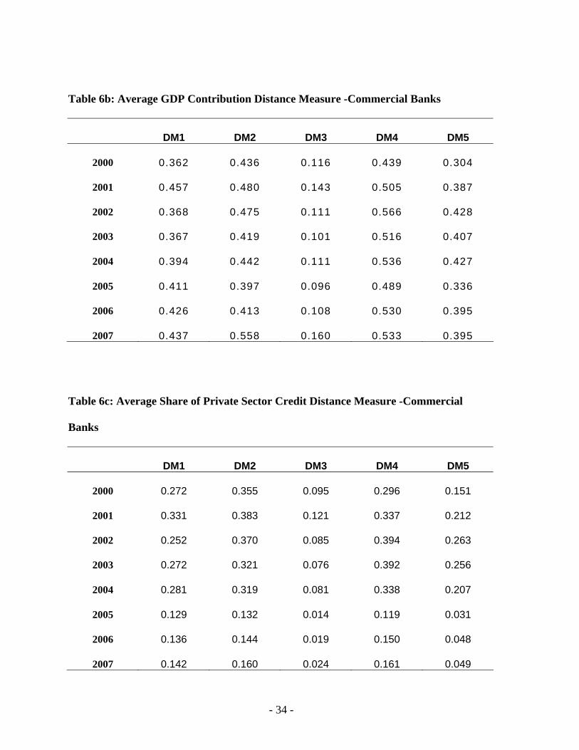
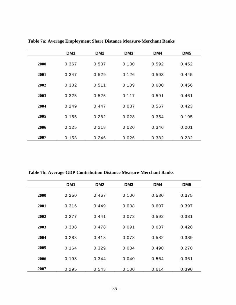
There were, however, mixed results for the average GDP contribution benchmark.
Commercial bank loan portfolios experienced a movement away from the GDP contribution
benchmark and hence increased sector concentration. Merchant banks and building societies,
on the other hand, had contradictory results. The merchant bank distance measures, DM2,
DM4 and DM5, diverge from the GDP contribution benchmark, whereas DM1 and DM3
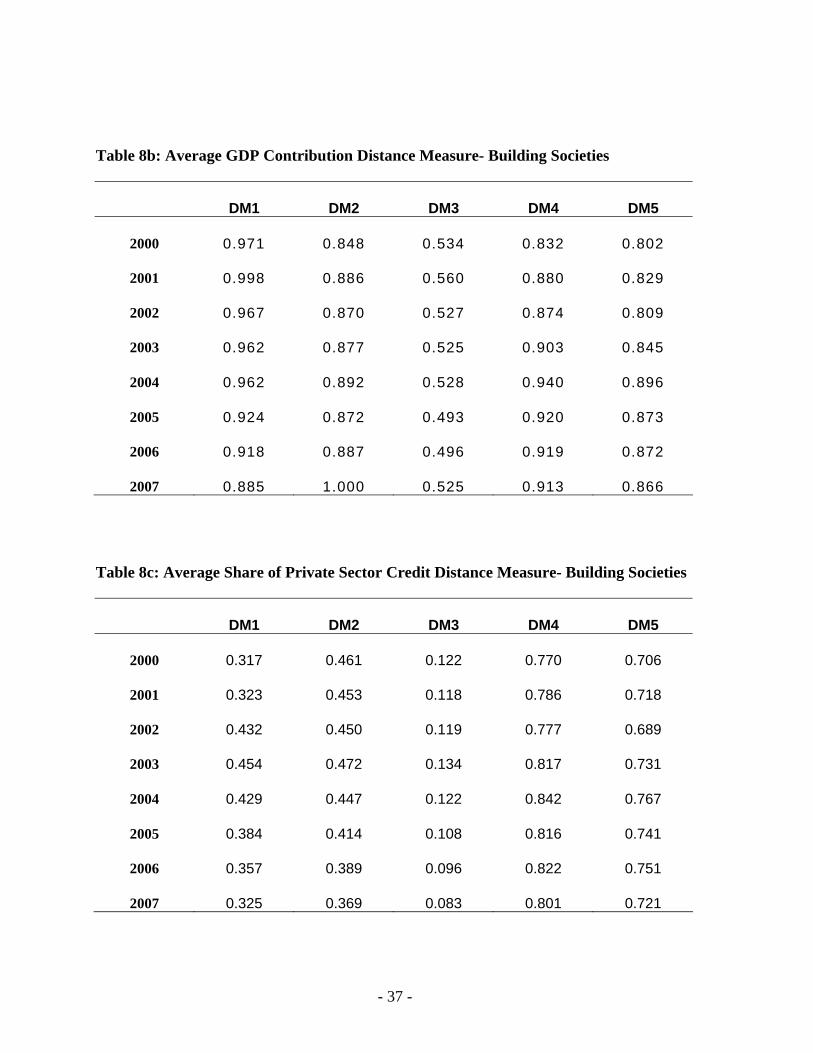
converge towards this benchmark. Building societies distance measures, DM1 and DM3,
converge towards the GDP contribution benchmark, whereas DM2, DM4 and DM5 diverge
away from this benchmark.12These results underscore the importance of the bank-level panel
regression analysis in determining the more accurate distance measures.
There was a convergence towards the average share of private sector lending benchmark for
all distance measures, with the exception of DM1, DM4 and DM5 of building societies
showing slight divergence. However, the values of the distance measures for the share of
10 See Table 4 in Appendix for Gini coefficient breakdown. 11 See Tables 5a, 6a, 7a and 8a in Appendix for distance measure results for the share of employment benchmark. 12 See Table 5b, 6b, 7b and 8b in Appendix for distance measure results for the GDP contribution benchmark.

- 11 -
private sector lending benchmark were significantly lower overall (hence, more diversified)
when compared to the values of the distance measures using the other two benchmarks.13
In summary, the distance measures indicate that commercial banks and merchant banks both
had loan portfolios of moderate concentration levels for the employment share per sector
benchmark and contribution to GDP per sector benchmark.14 In contrast, as expected, the
distance measures of building societies clearly indicate very concentrated loan portfolios.15
A correlation coefficient matrix was computed for each of individual distance measures per
economic sector benchmark. The low values of the matrix coefficients for the employment
share and GDP contribution benchmarks imply that the use of the five distance measures
should produce varied results in the empirical tests for their effect on bank return. However,
the correlation coefficients are positive and close to one in the case of the share of private
sector loans benchmark. This high degree of correlation among the distance measures is
expected to engender similar results in the empirical tests for their effects on bank return.16
6.0 Empirical Framework
The principal empirically testable hypotheses investigated in this study concern whether
there exists an efficient risk-return trade-off for bank-level loan portfolios and whether the
relationship between bank-level loan returns and loan portfolio diversification is non-linear
in bank-level risk. Portfolio theory assumes that there will be an inverse relationship between
portfolio risk and portfolio return when moving along the ‘efficient frontier.’ Further,
consistent with Winton’s (1999) seminal theoretical framework, there should be a non-linear
and U-shaped relationship between bank loan portfolio returns and loan portfolio risk.
6.1 Test of the Linear Effect of Concentration and Risk on Bank Returns
Consider the following panel regression equation to test the average effect of concentration
and risk on banks’ performance, using fixed effects estimation techniques:
13 See Table 5c, 6c, 7c and 8c in Appendix for distance measure results for the share of private sector lending benchmark. 14 See Tables 6a - 7b in Appendix. 15 See Tables 8a and b in Appendix. 16 See Tables 9a, b & c in Appendix.
- 12 -
[9] itmit
M
Nmmnit
N
nnitit ZXRiskturn εαααα ++∗+∗+= ∑∑
+== 1210Re
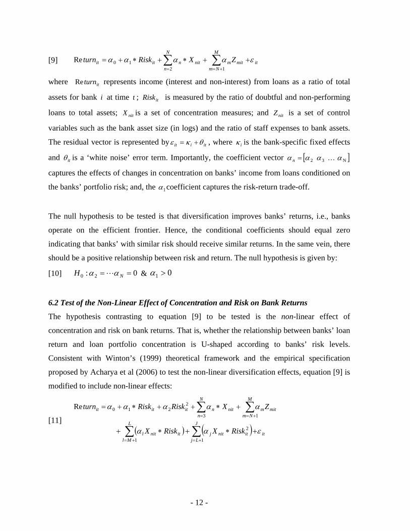
where itturnRe represents income (interest and non-interest) from loans as a ratio of total
assets for bank i at time t ; itRisk is measured by the ratio of doubtful and non-performing
loans to total assets; nitX is a set of concentration measures; and nitZ is a set of control
variables such as the bank asset size (in logs) and the ratio of staff expenses to bank assets.
The residual vector is represented by itiit θκε += , where iκ is the bank-specific fixed effects
and itθ is a ‘white noise’ error term. Importantly, the coefficient vector [ ]N32 αααα K=n
captures the effects of changes in concentration on banks’ income from loans conditioned on
the banks’ portfolio risk; and, the 1α coefficient captures the risk-return trade-off.
The null hypothesis to be tested is that diversification improves banks’ returns, i.e., banks
operate on the efficient frontier. Hence, the conditional coefficients should equal zero
indicating that banks’ with similar risk should receive similar returns. In the same vein, there
should be a positive relationship between risk and return. The null hypothesis is given by:
[10] 0: 20 == NH αα L & 01 >α
6.2 Test of the Non-Linear Effect of Concentration and Risk on Bank Returns
The hypothesis contrasting to equation [9] to be tested is the non-linear effect of
concentration and risk on bank returns. That is, whether the relationship between banks’ loan
return and loan portfolio concentration is U-shaped according to banks’ risk levels.
Consistent with Winton’s (1999) theoretical framework and the empirical specification
proposed by Acharya et al (2006) to test the non-linear diversification effects, equation [9] is
modified to include non-linear effects:
[11] ( ) ( ) it
J
Ljitnitj
L
Mlitnitl
mit
M
Nmmnit
N
nnititit
RiskXRiskX
ZXRiskRiskturn
εαα
ααααα
+∗+∗+
+∗++∗+=
∑∑
∑∑
+=+=
+==
1
2
1
13
2210
Re

- 13 -
Under the specification given by equation [9], the effect of concentration on banks’ returns is
non-linear in risk. This means that the first derivative of return on concentration using
equation [11] is given by:
[12] ( ) ( ) 23 *Re
)()( RiskRisk
Xturn
ionConcentratePerformanc
JjLlNnit
it αααααα +++∗++++=∂
∂=
∂∂
LLL
Therefore, the null hypothesis the effect of concentration on banks’ returns is U-shaped in
risk is given by:
[13] 0,, ;0,, ;0,,: jl30 ><>′ JLNH αααααα KKK
For the bank-level panel regressions, the concentration measures: DM1, DM1, DM3, DM4
and DM5 (as defined in Section 1) are computed in relation to each of the benchmarks: share
of employment per economic sector (EMP), contribution to gross domestic product (GDP)
per economic sector as well as share of total private sector lending per economic sector (PS).
Hence, in the case of each of the economic sector benchmarks computed in terms of
concentration measure DM1, equation [11] may be restated as:
[14]
( )
( ) ( )
( ) ( )
( ) itimit
M
Nmmitit
itititit
itititit
itit
ititititit
ZRiskPSDM
RiskGDPDMRiskEMPDM
RiskPSDMRiskGDPDM
RiskEMPDMPSDM
GDPDMEMPDMRiskRiskturn
θκαα
αα
αα
αα
ααααα
+++∗∗+
∗∗+∗∗+
∗∗+∗∗+
∗++
∗+∗++∗+=
∑+= 1
211
210
29
87
65
432
210
_1
_1_1
_1 _1
*_1_1*
_1_1Re
This specification implies that the first derivative of return on concentration according to the
EMP benchmark computed using the DM1 measure is given by:
[15] ( )
2963 *
_1Re
ititnit
it RiskRiskEMPDM
turnααα +∗+=
∂∂
If under the null hypothesis, the effect of bank i’s loan portfolio concentration on its returns
is U-shaped in risk, then:
[16] 0 ,0 ,0 ,0 ,0 ,0 : 118107960 ><><><′′ ααααααH .

- 14 -
An illustration of the pre-conditions under which the relationship between return and
concentration is a U-shaped function of the level of risk is presented in Acharya et al (2006).
In that study, the cumulative probability functions for two normal distributions are plotted,
with different standard deviations (risk levels) and a common mean (central tendency) of
zero. One distribution function, denoted as ‘less diversified’ has a standard deviation of 1.0
as the other ‘more diversified’ function has a lower standard deviation of 0.5. The authors
point out that if the level of debt is to the left of zero (central tendency), then a decrease in
standard deviation, by lowering the likelihood of events in the left (default) tail of the
distribution, reduces the probability of default. However, if the level of debt is to the right of
zero, then a decrease in standard deviation, by lowering the likelihood of events in the right
(no-default) tail of the distribution, increases the probability of default.
7.0 Preliminary Empirical Results
Preliminary empirical analyses were conducted by using the traditional and distance
measures computed in Section 1, along with risk and control variables, to determine the
evolution of loan portfolio concentration over the sample period by estimating fixed-effect
panel regressions with a time trend. Each diversification measure is regressed on a linear
trend variable:
[17] tb
tb timeDM εβα +∗+=
where DM tb represents the measure of diversification of bank b at time t.
Individual regressions were also run to ascertain the concentration behaviour of individual
banks over the review period using the following equation:
[18] tbbb
tb timeDM εβα +∗+=
7.1 Distance Measures Using Employment Share per Sector Benchmark
The trend coefficients of the panel using employment share by sector as a benchmark were
negative and significant for all distance measures (see Table 10). This signifies a reduction in
the distance between the loan portfolios and the employment benchmark over the sample
period. A reduction in the distance between loan portfolios and benchmarks reveal the
- 15 -
existence of increased diversification of private sector loan portfolios of the overall banking
sector over the period.
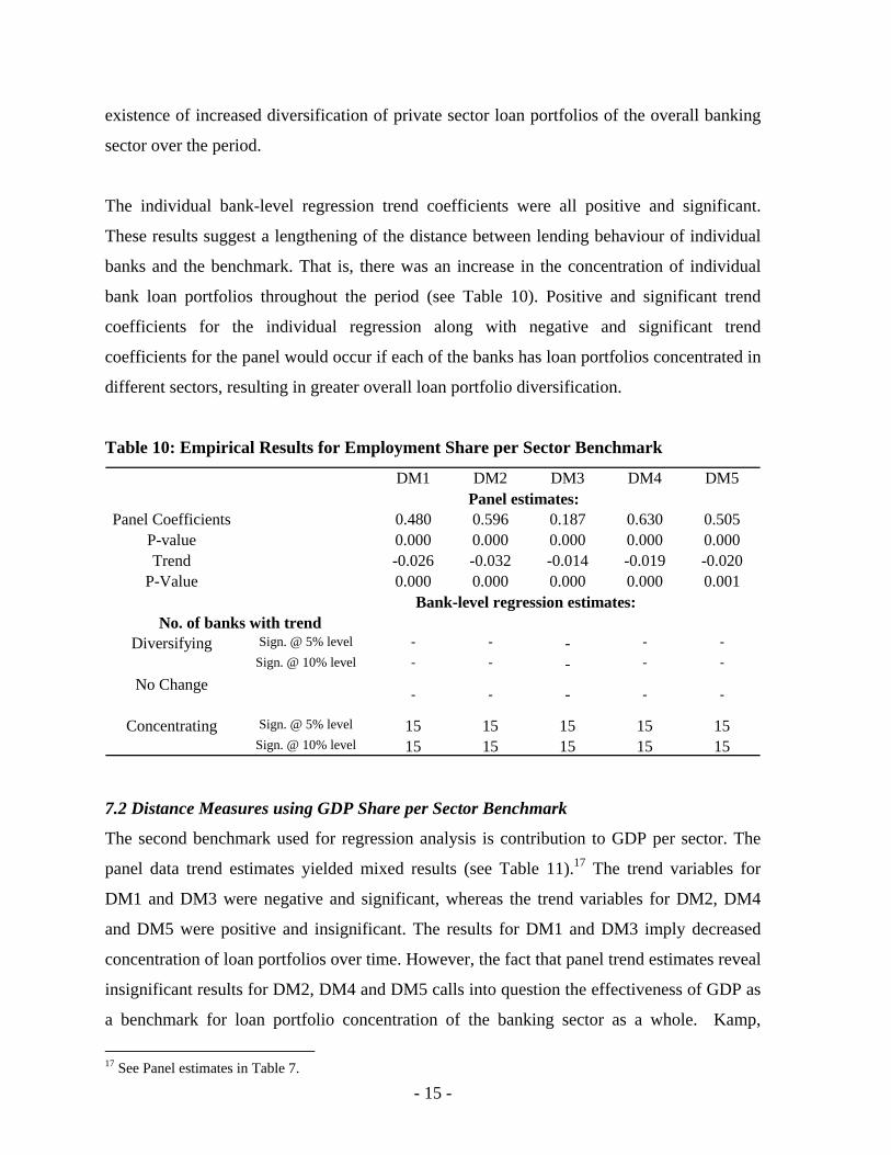
The individual bank-level regression trend coefficients were all positive and significant.
These results suggest a lengthening of the distance between lending behaviour of individual
banks and the benchmark. That is, there was an increase in the concentration of individual
bank loan portfolios throughout the period (see Table 10). Positive and significant trend
coefficients for the individual regression along with negative and significant trend
coefficients for the panel would occur if each of the banks has loan portfolios concentrated in
different sectors, resulting in greater overall loan portfolio diversification.
Table 10: Empirical Results for Employment Share per Sector Benchmark
DM1 DM2 DM3 DM4 DM5
Panel Coefficients 0.480 0.596 0.187 0.630 0.505P-value 0.000 0.000 0.000 0.000 0.000Trend -0.026 -0.032 -0.014 -0.019 -0.020
P-Value 0.000 0.000 0.000 0.000 0.001
Sign. @ 5% level - - - - -Sign. @ 10% level - - - - -
Sign. @ 5% level 15 15 15 15 15Sign. @ 10% level 15 15 15 15 15
-
Diversifying
No Change
Concentrating
Panel estimates:
Bank-level regression estimates:No. of banks with trend
- - - -
7.2 Distance Measures using GDP Share per Sector Benchmark
The second benchmark used for regression analysis is contribution to GDP per sector. The
panel data trend estimates yielded mixed results (see Table 11).17 The trend variables for
DM1 and DM3 were negative and significant, whereas the trend variables for DM2, DM4
and DM5 were positive and insignificant. The results for DM1 and DM3 imply decreased
concentration of loan portfolios over time. However, the fact that panel trend estimates reveal
insignificant results for DM2, DM4 and DM5 calls into question the effectiveness of GDP as
a benchmark for loan portfolio concentration of the banking sector as a whole. Kamp,
17 See Panel estimates in Table 7.
- 16 -
Pfingsten & Porath (2005) point out that low significance levels for trend variables, using
GDP share as a benchmark in regression analysis, could be occasioned by low correlations
between GDP and loan financing. In such a scenario, banks would not gauge their loan
exposures in accordance with GDP figures.
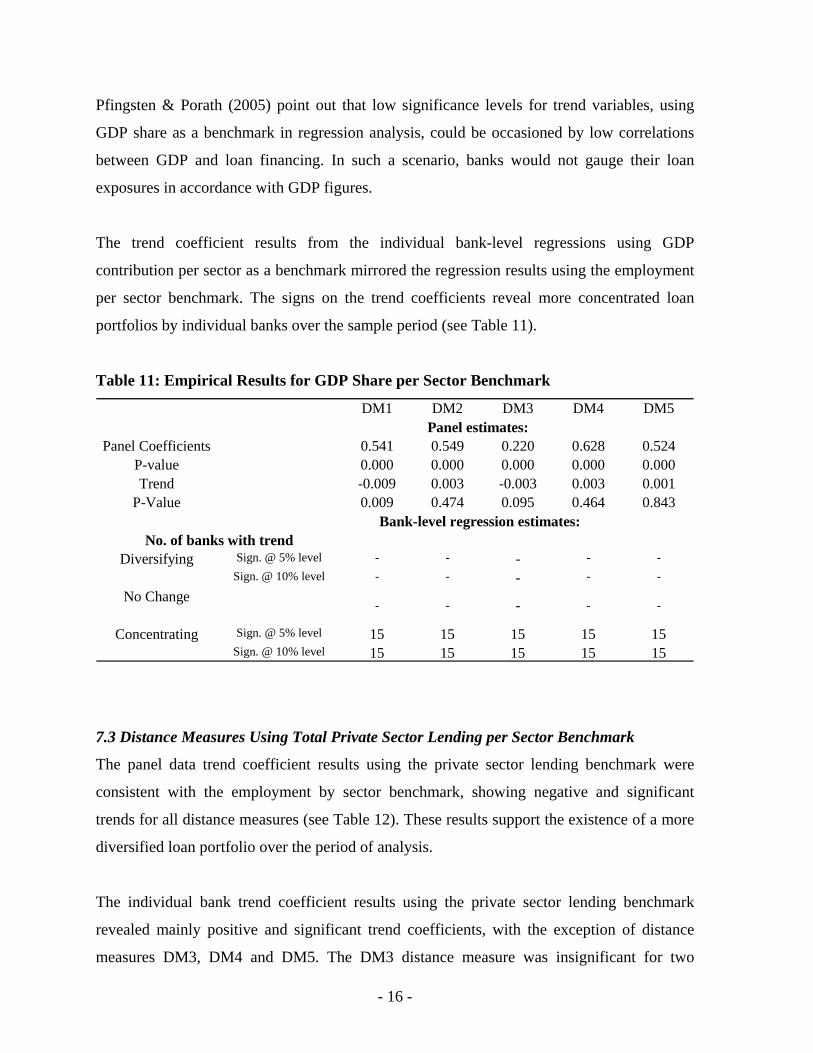
The trend coefficient results from the individual bank-level regressions using GDP
contribution per sector as a benchmark mirrored the regression results using the employment
per sector benchmark. The signs on the trend coefficients reveal more concentrated loan
portfolios by individual banks over the sample period (see Table 11).
Table 11: Empirical Results for GDP Share per Sector Benchmark
DM1 DM2 DM3 DM4 DM5
Panel Coefficients 0.541 0.549 0.220 0.628 0.524P-value 0.000 0.000 0.000 0.000 0.000Trend -0.009 0.003 -0.003 0.003 0.001
P-Value 0.009 0.474 0.095 0.464 0.843
Sign. @ 5% level - - - - -Sign. @ 10% level - - - - -
Sign. @ 5% level 15 15 15 15 15Sign. @ 10% level 15 15 15 15 15
-
Diversifying
No Change
Concentrating
Panel estimates:
Bank-level regression estimates:No. of banks with trend
- - - -
7.3 Distance Measures Using Total Private Sector Lending per Sector Benchmark
The panel data trend coefficient results using the private sector lending benchmark were
consistent with the employment by sector benchmark, showing negative and significant
trends for all distance measures (see Table 12). These results support the existence of a more
diversified loan portfolio over the period of analysis.
The individual bank trend coefficient results using the private sector lending benchmark
revealed mainly positive and significant trend coefficients, with the exception of distance
measures DM3, DM4 and DM5. The DM3 distance measure was insignificant for two

- 17 -
commercial bank regressions at the 5.0 per cent level of significance, whilst the results show
insignificant values for DM4 and DM5 in one of the commercial bank regressions (see Table
12).
Table 12: Empirical Results for Private Sector Lending per Sector Benchmark
DM1 DM2 DM3 DM4 DM5
Panel Coefficients 0.441 0.563 0.173 0.610 0.500P-value 0.000 0.000 0.000 0.000 0.000Trend -0.023 -0.038 -0.015 -0.024 -0.022
P-Value 0.000 0.000 0.000 0.000 0.000
Sign. @ 5% level - - - - -Sign. @ 10% level - - - - -
Sign. @ 5% level 15 15 13 14 14Sign. @ 10% level 15 15 15 14 14
1
Diversifying
No Change
Concentrating
Panel estimates:
Bank-level regression estimates:No. of banks with trend
- - 2 1
7.4 Traditional Concentration Measures
The panel estimates for HHI displayed an identical pattern to that of the employment per
sector benchmark and the private sector lending per sector benchmark. The estimates show
statistically significant and negative signs suggesting an increase in the degree of
diversification of banking sector loan portfolios over the review period. Conversely, the Gini
panel estimates are negative but statistically insignificant. These results illustrate the inability
of the Gini coefficient to measure concentration of loan portfolios of the overall banking
sector.
The regression results using the traditional concentration measures for the individual banks
correspond with those using the distance measures reflecting both employment share by
economic sector and contribution to GDP by economic sector. The concentration estimates
were all positive and significant. This confirms the increase in concentration of individual
loan portfolios over the period of analysis (see Table 13).
- 18 -
Table 13: Empirical Results for Traditional Measures
HHI Gini
Panel Trend -0.019 0.000P-Value 0.000 0.785
Sign. @ 5% level - -Sign. @ 10% level - -
Sign. @ 5% level 15 15Sign. @ 10% level 15 15
Diversifying
No Change
Concentrating
Panel estimates:
Bank-level regression estimates:No. of banks with trend
- -
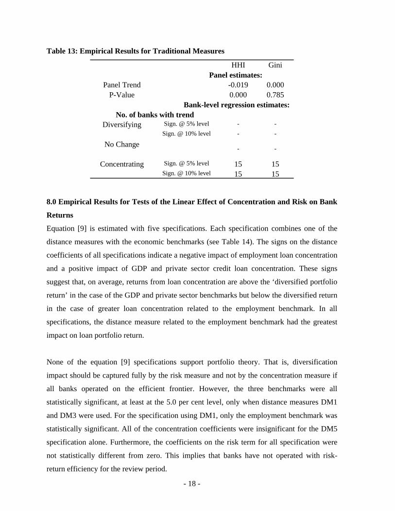
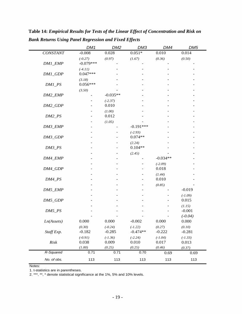
8.0 Empirical Results for Tests of the Linear Effect of Concentration and Risk on Bank
Returns
Equation [9] is estimated with five specifications. Each specification combines one of the
distance measures with the economic benchmarks (see Table 14). The signs on the distance
coefficients of all specifications indicate a negative impact of employment loan concentration
and a positive impact of GDP and private sector credit loan concentration. These signs
suggest that, on average, returns from loan concentration are above the ‘diversified portfolio
return’ in the case of the GDP and private sector benchmarks but below the diversified return
in the case of greater loan concentration related to the employment benchmark. In all
specifications, the distance measure related to the employment benchmark had the greatest
impact on loan portfolio return.
None of the equation [9] specifications support portfolio theory. That is, diversification
impact should be captured fully by the risk measure and not by the concentration measure if
all banks operated on the efficient frontier. However, the three benchmarks were all
statistically significant, at least at the 5.0 per cent level, only when distance measures DM1
and DM3 were used. For the specification using DM1, only the employment benchmark was
statistically significant. All of the concentration coefficients were insignificant for the DM5
specification alone. Furthermore, the coefficients on the risk term for all specification were
not statistically different from zero. This implies that banks have not operated with risk-
return efficiency for the review period.
- 19 -
Table 14: Empirical Results for Tests of the Linear Effect of Concentration and Risk on
Bank Returns Using Panel Regression and Fixed Effects DM1 DM2 DM3 DM4 DM5
-0.008 0.028 0.051* 0.010 0.014(-0.27) (0.97) (1.67) (0.36) (0.50)-0.079*** - - - -(-4.11) - - - -0.047*** - - - -(3.18) - - - -0.056*** - - - -(3.50) - - - -
- -0.035** - - -- (-2.37) - - -- 0.010 - - -- (1.00) - - -- 0.012 - - -- (1.05) - - -- - -0.191*** - -- - (-2.93) - -- - 0.074** - -- - (2.24) - -- - 0.104** - -- - (2.45) - -- - - -0.034** -- - - (-2.09) -- - - 0.018 -- - - (1.44) -- - - 0.010 -- - - (0.85) -- - - - -0.019- - - - (-1.09)- - - - 0.015- - - - (1.15)- - - - -0.001- - - - (-0.04)
0.000 0.000 -0.002 0.000 0.000(0.30) (-0.24) (-1.22) (0.27) (0.10)-0.182 -0.285 -0.474** -0.222 -0.281(-0.91) (-1.36) (-2.24) (-1.04) (-1.33)0.038 0.009 0.010 0.017 0.013(1.00) (0.25) (0.25) (0.46) (0.37)
R-Squared 0.71 0.71 0.70 0.69 0.69No. of obs. 113 113 113 113 113
Notes:1. t-statistics are in parentheses.2. ***, **, * denote statistical significance at the 1%, 5% and 10% levels.
Staff Exp.
DM5_PS
Risk
CONSTANT
DM1_EMP
Ln(Assets)
DM2_EMP
DM2_GDP
DM2_PS
DM1_GDP
DM3_EMP
DM3_GDP
DM3_PS
DM1_PS
DM5_EMP
DM5_GDP
DM4_EMP
DM4_GDP
DM4_PS

- 20 -
Table 15: Empirical Results for Tests of the Non-Linear Effect of Concentration and Risk
on Bank Returns Using Panel Regression and Fixed Effects DM1 DM2 DM3 DM4 DM5
-0.036 -0.041 -0.015 -0.026 -0.011(-1.11) (-0.42) (-0.89) (-0.32)-0.162*** - - - -(-4.54) - - - -6.697** - - - -(2.61) - - - --55.208* - - - -(-1.84) - - - -0.106*** - - - -(3.67) - - - --3.927* - - - -(-2.33) - - - -30.464 - - - -(1.65) - - - -0.118*** - - - -(4.17) - - - --4.940*** - - - -(-2.70) - - - -44.352** - - - -(2.23) - - - -
- -0.080*** - - -- (-3.55) - - -- 3.010** - - -- (2.28) - - -- -21.865* - - -- (-1.68) - - -- 0.036** - - -- (2.16) - - -- -1.436 - - -- (-1.65) - - -- 10.197 - - -- (1.15) - - -- 0.045** - - -- (2.53) - - -- -2.509** - - -- (-2.46) - - -- 27.802** - - -- (2.34) - - -- - -0.482*** - -- - (-4.39) - -- - 14.564** - -- - (2.62) - -- - -95.819* - -- - (-1.82) - -- - 0.203*** - -- - (3.40) - -- - -6.630** - -- - (-2.31) - -- - 42.507 - -- - (1.57) - -- - 0.283*** - -- - (4.05) - -- - -9.566*** - -- - (-2.61) - -- - 78.073* - -- - (1.88) - -
(continued overleaf)
DM3_GDPRISKSQ
DM3_PS
DM3_PSRISK
DM3_PSRISKSQ
DM3_EMPRISK
DM3_EMPRISKSQ
DM3_GDP
DM3_GDPRISK
DM2_PS
DM2_PSRISK
DM2_PSRISKSQ
DM3_EMP
CONSTANT
DM2_GDP
DM2_GDPRISK
DM2_GDPRISKSQ
DM1_PSRISKSQ
DM2_EMP
DM2_EMPRISK
DM2_EMPRISKSQ
DM1_GDPRISK
DM1_GDPRISKSQ
DM1_PS
DM1_PSRISK
DM1_EMP
DM1_EMPRISK
DM1_EMPRISKSQ
DM1_GDP
- 21 -
Table 15 (continued): Empirical Results for Tests of the Non-Linear Effect of
Concentration and Risk on Bank Returns Using Panel Regression and Fixed Effects DM1 DM2 DM3 DM4 DM5
- - - -0.112*** -- - - (-4.65) -- - - 7.000*** -- - - (3.95) -- - - -64.707*** -- - - (-3.05) -- - - 0.046** -- - - (2.55) -- - - -0.46 -- - - (-0.36) -- - - -18.481 -- - - (-0.91) -- - - 0.074*** -- - - (4.04) -- - - -6.306*** -- - - (-4.32) -- - - 77.428*** -- - - (3.82) -- - - - -0.054**- - - - (-2.06)- - - - 3.465- - - - (1.58)- - - - -32.410- - - - (-1.10)- - - - 0.035*- - - - (1.73)- - - - -1.501- - - - (-0.92)- - - - 9.248- - - - (0.34)- - - - 0.024- - - - (1.18)- - - - -2.341- - - - (-1.59)- - - - 25.045- - - - (1.23)
0.001 0.003 0.001 0.002 0.001(0.57) (1.52) -0.46 (1.22) (0.66)-0.146 0.117 -0.041 -0.031 -0.146(-0.61) (0.47) (-0.167) (-0.14) (-0.58)1.102** 0.539 0.606* -0.328 0.268(2.08) (1.26) (1.81) (-0.78) (0.75)-8.770* -7.235 -4.846 8.705 -0.878(-1.69) (-1.34) (-1.17) (1.62) (-0.18)
R-Squared 0.75 0.74 0.75 0.75 0.70No. of obs. 113 113 113 113 113
Notes:1. t-statistics are in parentheses.2. ***, **, * denote statistical significance at the 1%, 5% and 10% levels.
Ln(Assets)
Staff Expenses
Risk
Risk Squared
DM5_GDPRISKSQ
DM5_PS
DM5_PSRISK
DM5_PSRISKSQ
DM5_EMPRISK
DM5_EMPRISKSQ
DM5_GDP
DM5_GDPRISK
DM4_PS
DM4_PSRISK
DM4_PSRISKSQ
DM5_EMP
DM4_EMPRISKSQ
DM4_GDP
DM4_GDPRISK
DM4_GDPRISKSQ
DM4_EMP
DM4_EMPRISK

- 22 -
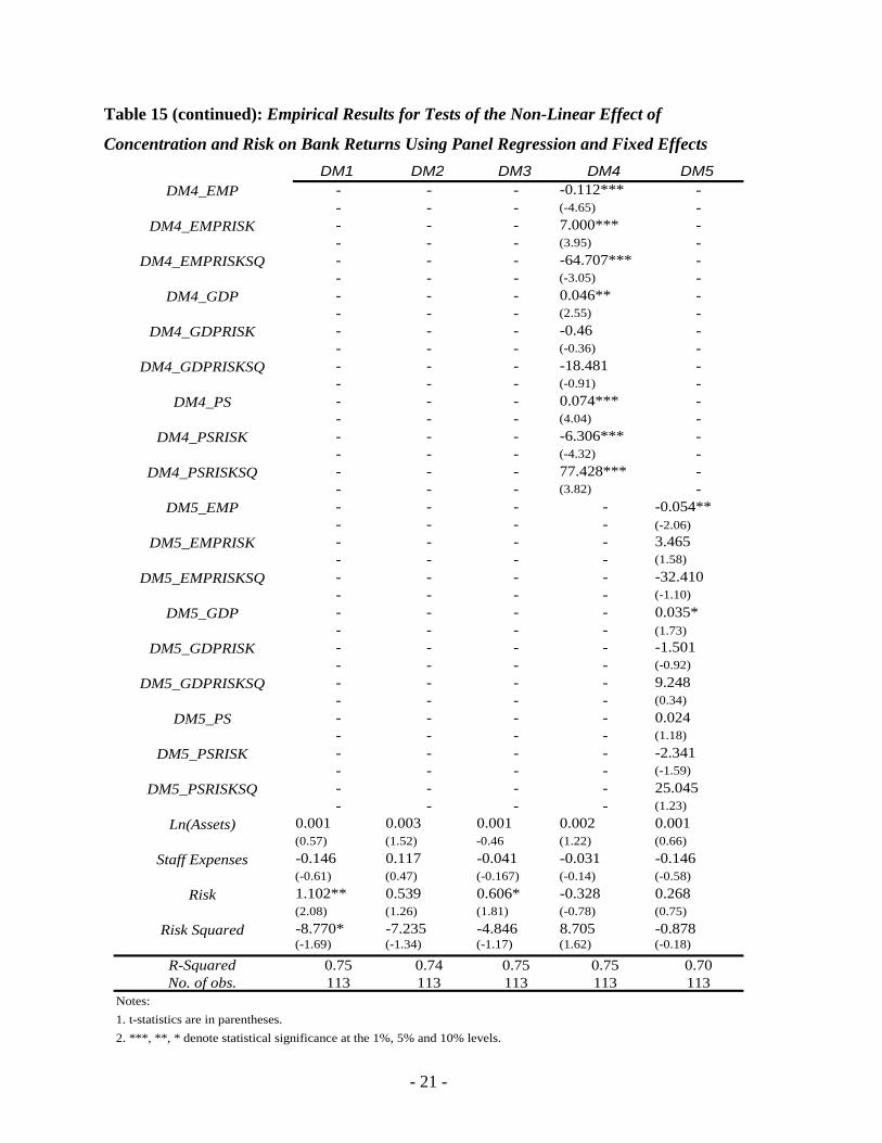
Equation [9] is modified by the inclusion of interaction variables between the distance
measures and the risk measure as well as between the distance measures and the risk squared
measure, as represented by equation [11]. The estimation results of equation [11] support the
existence of a non-linear effect of loan concentration and risk on bank loan returns (see Table
15). That is, the results from estimating the modified version of equation [9] do not support
the view of traditional portfolio theory. The results from this non-linear regression equation
indicate that the relationship between banks’ loan return and loan portfolio concentration is
U-shaped according to banks’ risk levels, in the case of the GDP and private sector
benchmarks, and has an inverted U-shape in the case of the employment benchmark.
Specifically, in the case of the GDP and private sector credit benchmarks, the coefficients on
the interaction terms between these benchmarks and risk and the benchmarks and risk
squared are negative and positive, respectively, and are statistically significant at least at the
10.0 per cent level. The opposite signs are obtained on the interaction terms in the case of the
employment benchmark.
In addition, similar to the results from estimating equation [9], the sign and statistical
significance of linear coefficients in equation [11] provide further support for the benefits of
diversification in the case of the employment benchmark but against the benefits of
diversification in the cases of the GDP and private sector credit benchmarks. Furthermore,
the coefficient on the risk measure in the cases of the latter two measures is positive and
significant in the specifications employing the DM1 and DM3 concentration measures.
However, the coefficient on risk-squared measure is negative and significant when the DM1
measure is used, providing further evidence of a non-linear risk return relationship.
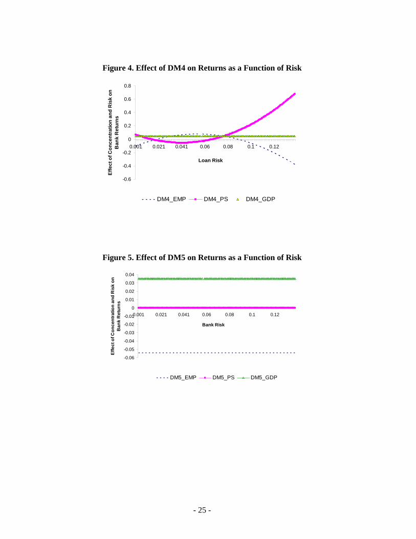
To illustrate the economic implications of the non-linear effect of concentration and risk on
bank loan returns, the marginal effects for all three economic benchmarks are plotted for
different values of risk. The marginal effects for the distance measures,
ionConcentratePerformanc ∂∂ , are graphed using the coefficients on these distance measures
and their interaction terms with the risk measure from the non-linear panel regressions (see
Table 15 and Figures 1 to 5). The range of risk used in the graphs lies between the minimum
and maximum values of the doubtful and nonperforming loans ratio covered over the sample
period.

- 23 -
The coefficients on distance measures and their interactions are all statistically significant
only for the regressions using distance measure DM1 and DM3 (see Table 15, Figures 1 and
Figure 3). As evidenced in corresponding figures, the marginal effects using the GDP
contribution and private sector credit share benchmarks are positive and declining at low risk
levels (within the approximate range of 0 to 4.0 per cent), are close to zero at moderate risk
levels and are positive and rising at high risk levels (approximately greater than 8.0 per cent).
In the case of the private sector share benchmark, the marginal effects display a sharper
monotonic decline and increase relative to the GDP contribution benchmark. In contrast (but
consistent with portfolio theory), the marginal effects using the employment share
benchmark is negative and increasing at low risk levels, is close to zero at moderate risk
levels and is negative and declining at high risk levels.
Figure 1. Effect of DM1 on Returns as a Function of Risk
-0.4
-0.3
-0.2
-0.1
0
0.1
0.2
0.3
0.4
0.001 0.021 0.041 0.06 0.08 0.1 0.12
Loan Risk
Effe
ct o
f Con
cent
ratio
n an
d R
isk
on
Ban
k R
etur
ns
DM1_EMP DM1_PS DM1_GDP

- 24 -
Figure 2. Effect of DM2 on Returns as a Function of Risk
-0.1
-0.05
0
0.05
0.1
0.15
0.2
0.25
0.001 0.021 0.041 0.06 0.08 0.1 0.12
Loan Risk
Effe
ct o
f Con
cent
ratio
n an
d R
isk
on
Ban
k R
etur
ns
DM2_EMP DM2_PS DM2_GDP
Figure 3. Effect of DM3 on Returns as a Function of Risk
-0.6
-0.4
-0.2
0
0.2
0.4
0.6
0.001 0.021 0.041 0.061 0.081 0.101 0.121
Loan Risk
Effe
ct o
f Con
cent
ratio
n an
d R
isk
on
Ban
k R
etur
ns
DM3_EMP DM3_PS DM3_GDP
- 25 -
Figure 4. Effect of DM4 on Returns as a Function of Risk
-0.6
-0.4
-0.2
0
0.2
0.4
0.6
0.8
0.001 0.021 0.041 0.06 0.08 0.1 0.12
Loan Risk
Effe
ct o
f Con
cent
ratio
n an
d R
isk
on
Ban
k R
etur
ns
DM4_EMP DM4_PS DM4_GDP
Figure 5. Effect of DM5 on Returns as a Function of Risk
-0.06
-0.05
-0.04
-0.03
-0.02
-0.01
0
0.01
0.02
0.03
0.04
0.001 0.021 0.041 0.06 0.08 0.1 0.12
Bank Risk
Effe
ct o
f Con
cent
ratio
n an
d R
isk
on
Ban
k R
etur
ns
DM5_EMP DM5_PS DM5_GDP

- 26 -
9. Discussion and Conclusion
Panel and individual bank-level regressions were run to determine the movements in
concentration of loan portfolios of the overall banking sector and individual banks over 2000
to 2007. The panel results showed increased diversification of loan portfolios of the overall
banking sector over the sample period as evidenced by negative and significant trend
estimates using the distance as well as traditional measures.
However, the results from the individual bank-level regressions provide strong evidence of
movement towards higher concentration of loan portfolios over the review period for all
measures of distance and concentration. These results supported the findings from
preliminary data analysis indicating that private sector lending was slightly more
concentrated in 2007 relative to 2000, with increases in the loan proportions to the personal
sector and, to a lesser extent, Tourism, Distribution & Entertainment. In addition,
commercial banks and merchant banks focused their portfolios on personal loans, Tourism,
Distribution & Entertainment and the Professional & Other Services. Building societies
remained significantly concentrated in personal loans.
The key result of the paper is that bank-level panel regression tests of the linear and non-
linear effects of concentration and risk on bank returns support the hypothesis that greater
diversification does not imply lower risk and/or greater returns. The Maximum Absolute
Differences (DM1) and Normalized Sum of Squared Differences (DM3) were the most
effective of the distance measures in reflecting this result. Specifically, the results indicate
that returns from loan concentration are above the diversified portfolio return in the case of
the GDP contribution and private sector credit share benchmarks but below the diversified
return in the case of greater loan concentration related to the employment share benchmark.
Hence, the relationship between banks’ loan return and loan portfolio concentration is U-
shaped according to banks’ risk levels, in the case of the GDP and private sector benchmarks
and has an inverted U-shape in the case of the employment benchmark. In conclusion,
contrary to traditional portfolio theory, concentration rather then diversification of bank-level
loan portfolios may be more consistent with achieving minimal systemic risk.

- 27 -
References
Acharya, V., I. Hasan and A. Saunders (2006), “Should Banks be Diversified? Evidence
from Individual Bank Loan Portfolios,” Journal of Business, 79 (3), pp. 1355-1413.
Dell’ Ariccia, G., E. Friedman and R. Marquez, (1999), “Adverse Selection as a Barrier to
Entry in the Banking Industry,” European Economic Review, 45, pp. 1957-1980.
Deng, S. and E. Elyasiani (2007), “Diversification and Performance of U.S. Commercial
Banks,” April 2007.
Diamond, D. (1984), “Financial Intermediation and Delegated Monitoring”, Review of
Economic Studies, 51, pp. 393-414.
Dullman, K. and N Masschelein (2006), “Sector Concentration in Loan Portfolios and
Economic Capital,” National Bank of Belgium, Working paper research No. 105,
November, 2006.
Elyasiani E. and S. Deng (2004),”Diversification Effects on the Performance of Financial
Services Firms,” Working Paper, Temple University, Philadelphia.
Hayden, E., D. Porath and N. von Westernhagen (2006), “Does Diversification Improve the
Performance of German Banks? Evidence from Individual Bank Loan Portfolios,”
Discussion Paper, Series 2: Banking and Financial Studies, No. 05. Deutsche
Bundesbank.
Heitfield, E., S. Burton and S. Chomsisengphet (2005), “The Effects of Name and Sector
Concentration on the Distribution of Losses for Portfolios of Large Wholesale Credit
Exposures,” October 2005.
Kamp, A., A Pfingsten and D. Porath (2005), “Do Banks Diversify Loan Portfolios? A
Tentative Answer based on Individual Bank Loan Portfolios,” Deutsche Bundesbank,
Discussion Paper, Series 2: Banking and Financial Studies, No. 03/2005.

- 28 -
McElligot, R and R. Stuart (2007), “Measuring the Sectoral Distribution of Lending to Irish
Non-Financial Corporates,” Central Bank & Financial Services Authority of Ireland,
Financial Stability Report 2007.
Pfingsten, A. and K. Rudolph (2002), “German Banks' Loan Portfolio Composition: Market-
Orientation Vs. Specialisation,” Tech. Rep. 02-02, Institut für Kreditwesen, Münster.
Stomper, A. (2004), “A Theory of Banks’ Industry Expertise, Market Power, and Credit
Risk,” University of Vienna.
Winton, A. (1999), “Don’t Put All Your Eggs in One Basket? Diversification and
Specialization in Lending,” Finance Department, University of Minnesota,
Minneapolis.

- 29 -
Appendix
Table 1: Economic Sub-sectors
Sub-Sectors Private Sector Credit Share
per Sector (%)
Contribution to GDP per Sector
(%)*18
Employment share per sector (%)
2000 2007 2000 2007 2000 2007
AGRICULTURE & FISHING 3.65 1.43 6.69 34.17 20.96 17.38
MINING, QUARRYING & PROC. 0.23 0.23 4.36 5.50 0.50 0.68
MANUFACTURING 8.36 3.11 13.73 12.60 7.46 6.06
CONSTRUCTION & LAND DEV. 7.78 5.94 9.78 10.70 8.72 10.27
TRANSPORT, STORAGE & COMM. 3.52 4.02 11.66 14.20 6.36 6.29
TOURISM, DISTR & ENTERTAINMENT 20.26 22.85 28.63 31.50 22.10 23.14
PROFESSIONAL & OTHER SERVICES 13.36 6.52 6.10 5.30 5.69 6.74
PERSONAL & NON BUS. LOANS 55.29 56.51 0.63 0.45 27.29 28.58
ELECTRICITY 1.87 1.08 3.43 4.10 0.67 0.67
18 Financial services & Insurance services as well as Government services have been excluded from the study. Additionally, there were no imputed service charges figures available for 2007.

- 30 -
Table 2: List of Banks
Financial Institution Type
Bank of Nova Scotia Commercial Bank
National Commercial Bank Commercial Bank
Royal Bank of Trinidad and Tobago Commercial Bank
First Caribbean International Bank Commercial Bank
First Global Bank Commercial Bank
CitiBank National Commercial Bank
MF&G Merchant Bank
Capital & Credit Merchant Bank Merchant Bank
Pan Caribbean Merchant Bank Merchant Bank
Dehring, Bunting & Golding Merchant Bank
Citi Merchant Merchant Bank
Victoria Mutual Building Society Building Society
Jamaica National Building Society Building Society
Scotia Jamaica Building Society Building Society
First Caribbean International Building Society Building Society

- 31 -
Table 3: HHI
Date 2000 2001 2002 2003 2004 2005 2006 2007
HHI - Overall 0.552 0.554 0.528 0.527 0.528 0.528 0.535 0.534
HHI
- Commercial Banks 0.378 0.384 0.304 0.300 0.306 0.306 0.326 0.323
HHI - Merchant Banks 0.312 0.328 0.323 0.331 0.282 0.173 0.178 0.176
HHI
- Building Societies 0.967 1.013 0.978 0.941 0.932 0.87 0.858 0.809
Table 4: Gini Coefficient
Date 2000 2001 2002 2003 2004 2005 2006 2007
Gini - Overall 0.323 0.34 0.34 0.342 0.342 0.344 0.35 0.348
Gini -Commercial Banks 0.238 0.288 0.29 0.294 0.294 0.302 0.318 0.313
Gini
- Merchant Banks 0.303 0.308 0.302 0.313 0.287 0.236 0.259 0.249
Gini - Building Societies 0.428 0.434 0.432 0.436 0.412 0.438 0.438 0.437

- 32 -
Table 5a: Average Employment Distance Measure
DM1 DM2 DM3 DM4 DM5
2000 0.465 0.548 0.160 0.576 0.455
2001 0.480 0.545 0.185 0.508 0.486
2002 0.423 0.53 0.159 0.622 0.496
2003 0.429 0.522 0.158 0.625 0.509
2004 0.401 0.493 0.148 0.62 0.498
2005 0.317 0.386 0.105 0.494 0.367
2006 0.318 0.377 0.103 0.509 0.388
2007 0.317 0.387 0.099 0.526 0.397
Table 5b: Average GDP Contribution Distance Measure
DM1 DM2 DM3 DM4 DM5
2000 0.561 0.584 0.250 0.617 0.494
2001 0.590 0.605 0.264 0.664 0.538
2002 0.537 0.595 0.239 0.677 0.539
2003 0.546 0.591 0.239 0.685 0.56
2004 0.546 0.582 0.237 0.686 0.571
2005 0.499 0.533 0.207 0.636 0.496
2006 0.514 0.548 0.215 0.671 0.543
2007 0.539 0.705 0.262 0.687 0.550

- 33 -
Table 5c: Average Share of Private Sector Credit Distance Measure
DM1 DM2 DM3 DM4 DM5
2000 0.353 0.469 0.137 0.544 0.426
2001 0.38 0.484 0.148 0.583 0.467
2002 0.376 0.475 0.129 0.599 0.478
2003 0.383 0.46 0.13 0.597 0.479
2004 0.376 0.431 0.121 0.591 0.479
2005 0.299 0.309 0.072 0.453 0.341
2006 0.286 0.291 0.066 0.456 0.343
2007 0.270 0.272 0.063 0.471 0.351
Table 6a: Average Employment Share Distance Measure-Commercial Banks
DM1 DM2 DM3 DM4 DM5
2000 0.323 0.447 0.049 0.361 0.198
2001 0.366 0.417 0.111 0.422 0.277
2002 0.272 0.406 0.078 0.458 0.321
2003 0.273 0.361 0.070 0.432 0.302
2004 0.268 0.344 0.069 0.408 0.260
2005 0.150 0.236 0.027 0.263 0.120
2006 0.189 0.251 0.033 0.309 0.166
2007 0.195 0.276 0.038 0.333 0.176
- 34 -
Table 6b: Average GDP Contribution Distance Measure -Commercial Banks
DM1 DM2 DM3 DM4 DM5
2000 0.362 0.436 0.116 0.439 0.304
2001 0.457 0.480 0.143 0.505 0.387
2002 0.368 0.475 0.111 0.566 0.428
2003 0.367 0.419 0.101 0.516 0.407
2004 0.394 0.442 0.111 0.536 0.427
2005 0.411 0.397 0.096 0.489 0.336
2006 0.426 0.413 0.108 0.530 0.395
2007 0.437 0.558 0.160 0.533 0.395
Table 6c: Average Share of Private Sector Credit Distance Measure -Commercial
Banks
DM1 DM2 DM3 DM4 DM5
2000 0.272 0.355 0.095 0.296 0.151
2001 0.331 0.383 0.121 0.337 0.212
2002 0.252 0.370 0.085 0.394 0.263
2003 0.272 0.321 0.076 0.392 0.256
2004 0.281 0.319 0.081 0.338 0.207
2005 0.129 0.132 0.014 0.119 0.031
2006 0.136 0.144 0.019 0.150 0.048
2007 0.142 0.160 0.024 0.161 0.049
- 35 -
Table 7a: Average Employment Share Distance Measure-Merchant Banks
DM1 DM2 DM3 DM4 DM5
2000 0.367 0.537 0.130 0.592 0.452
2001 0.347 0.529 0.126 0.593 0.445
2002 0.302 0.511 0.109 0.600 0.456
2003 0.325 0.525 0.117 0.591 0.461
2004 0.249 0.447 0.087 0.567 0.423
2005 0.155 0.262 0.028 0.354 0.195
2006 0.125 0.218 0.020 0.346 0.201
2007 0.153 0.246 0.026 0.382 0.232
Table 7b: Average GDP Contribution Distance Measure-Merchant Banks
DM1 DM2 DM3 DM4 DM5
2000 0.350 0.467 0.100 0.580 0.375
2001 0.316 0.449 0.088 0.607 0.397
2002 0.277 0.441 0.078 0.592 0.381
2003 0.308 0.478 0.091 0.637 0.428
2004 0.283 0.413 0.073 0.582 0.389
2005 0.164 0.329 0.034 0.498 0.278
2006 0.198 0.344 0.040 0.564 0.361
2007 0.295 0.543 0.100 0.614 0.390

- 36 -
Table 7c: Average Share of Private Sector Credit Distance Measure-Merchant Banks
DM1 DM2 DM3 DM4 DM5
2000 0.471 0.591 0.195 0.565 0.421
2001 0.487 0.616 0.207 0.625 0.473
2002 0.445 0.604 0.184 0.627 0.483
2003 0.423 0.586 0.179 0.581 0.450
2004 0.418 0.527 0.161 0.593 0.463
2005 0.384 0.382 0.094 0.425 0.251
2006 0.364 0.340 0.081 0.396 0.229
2007 0.344 0.287 0.080 0.451 0.282
Table 8a: Average Employment Share Distance Measure- Building Societies
DM1 DM2 DM3 DM4 DM5
2000 0.704 0.660 0.301 0.775 0.715
2001 0.726 0.687 0.316 0.814 0.737
2002 0.694 0.672 0.291 0.809 0.711
2003 0.689 0.680 0.288 0.851 0.763
2004 0.687 0.688 0.288 0.886 0.812
2005 0.645 0.661 0.260 0.863 0.787
2006 0.641 0.661 0.258 0.871 0.796
2007 0.604 0.639 0.234 0.862 0.784
- 37 -
Table 8b: Average GDP Contribution Distance Measure- Building Societies
DM1 DM2 DM3 DM4 DM5
2000 0.971 0.848 0.534 0.832 0.802
2001 0.998 0.886 0.560 0.880 0.829
2002 0.967 0.870 0.527 0.874 0.809
2003 0.962 0.877 0.525 0.903 0.845
2004 0.962 0.892 0.528 0.940 0.896
2005 0.924 0.872 0.493 0.920 0.873
2006 0.918 0.887 0.496 0.919 0.872
2007 0.885 1.000 0.525 0.913 0.866
Table 8c: Average Share of Private Sector Credit Distance Measure- Building Societies
DM1 DM2 DM3 DM4 DM5
2000 0.317 0.461 0.122 0.770 0.706
2001 0.323 0.453 0.118 0.786 0.718
2002 0.432 0.450 0.119 0.777 0.689
2003 0.454 0.472 0.134 0.817 0.731
2004 0.429 0.447 0.122 0.842 0.767
2005 0.384 0.414 0.108 0.816 0.741
2006 0.357 0.389 0.096 0.822 0.751
2007 0.325 0.369 0.083 0.801 0.721

- 38 -
Table 9a: Correlation coefficients: Employment Share Benchmark
DM1 DM2 DM3 DM4 DM5
DM1
1
DM2 0.980
1
DM3 0.980 0.972
1
DM4 0.472 0.620 0.496
1
DM5 0.828 0.889 0.879 0.799
1
Table 9b: Correlation coefficients: GDP Contribution Benchmark
DM1 DM2 DM3 DM4 DM5
DM1
1
DM2 0.384
1
DM3 0.857 0.795
1
DM4 0.031 0.443 0.184
1
DM5 0.182 0.372 0.238 0.954 1 Table 9c: Correlation coefficients: Share of Private Sector Lending Benchmark
DM1 DM2 DM3 DM4 DM5
DM1
1
DM2 0.964
1
DM3 0.950 0.991
1
DM4 0.964 0.926 0.909
1
DM5 0.972 0.927 0.911 0.998
1
Top Related