Measurement Error in Survey Data:

An Application to a Model of Job Mobility in Ireland

By Adele Bergin1

(National University of Ireland, Maynooth and Economic and Social Research Institute, Dublin)

Paper Prepared for the 12th IZA European Summer School

This Draft: April 19th, 2009

Abstract Many studies of labour market dynamics use survey data so it is valuable to know about the quality of the data collected. This paper investigates job mobility in Ireland over the period 1995 to 2001, using the Living in Ireland Survey, the Irish component of the European Community Household Panel. As is common with many Surveys, there is no direct question about changing jobs; instead mobility is inferred from responses of individuals to a question about tenure on two adjacent interview dates. The paper finds that there is substantial inconsistencies or measurement error in the responses used to determine job changes so there is a risk of misclassifying cases as being job changes when truly no change took place and vice versa. The extent of measurement error is similar to what has been found in other studies (e.g. Brown and Light, 1992). Any technique used to estimate the determinants of job change should control for misclassification error, otherwise it can lead to estimates that are biased and inconsistent. A procedure proposed by Hausman, Abrevaya and Scott-Morton (1998) is used to control for misclassification. The paper finds that ignoring misclassification may substantially underestimate the true number of job changes. In addition, ignoring misclassification leads to diminished covariate effects in models of job change. JEL classification: J62 Keywords: Job Mobility; Binary choice model; Response Error

1 Email: Adele.Bergin@esri.ie

1

1. Introduction Many studies of labour market dynamics use survey data. Therefore it is valuable to know about the quality of the data collected. There may be ambiguity in a survey question, respondents may misunderstand the question, they may have poor recall or responses may be coded incorrectly. This paper investigates job mobility or employment-to-employment transitions in Ireland over the period 1995 to 2001 using the Living in Ireland Survey (LIS), the Irish component of the European Community Household Panel (ECHP). There is no direct question in the LIS about job mobility; instead it is inferred from responses of individuals on two adjacent interview dates. The paper finds that there is substantial measurement error in the data which may lead to misclassifying people who have not changed jobs as having changed jobs and vice versa. Any technique used to estimate the determinants of job mobility should control for misclassification error, otherwise it can lead to estimates that are biased and inconsistent. A procedure proposed by Hausman, Abrevaya and Scott-Morton (1998) is used to control for misclassification in the dependent variable. This paper is organised as follows: Section 2 examines the reasons for and prevalence of reporting errors in labour market survey data and, in particular, focuses on studies relevant to job mobility. Section 3 explores the extent of measurement error in the LIS data. Section 4 outlines the estimation technique used to control for misclassification. Section 5 presents a simple extension of the estimation technique that allows for covariate-dependent measurement error. Section 6 provides estimation results and Section 7 concludes.

2. Labour Market Survey Data Most studies of job mobility use survey data and usually surveys do not contain a direct question asking if the respondent has changed jobs in the past year. Instead job changes are inferred from the length of time an employee reports to have been with their current employer. Therefore questions about tenure play a crucial role in most empirical studies of job mobility. There are several reasons to suspect that responses to questions about tenure are measured with error. Respondents may find it difficult to remember when they started working in their current job. Bound et al. (2001) describe studies that categorise the question and answer process in a survey as a four-stage procedure. These stages include understanding the question, recovering the information from memory, considering whether the information matches what was requested and communicating the response. Much of the measurement error literature focuses on the stage where respondents retrieve the information from memory. A general principle from this literature is that the longer the length of the recall period the greater the expected bias due to respondent retrieval error. Therefore we might expect respondents with longer tenure to be most likely to misreport tenure. In one sense, this does not pose a serious problem for calculating job changes as job changes are associated with people who have short tenures; provided those with longer tenures who misreport do not significantly underestimate their tenure. Farber (1999) and Ureta (1992) find a heaping of tenure responses at round counts of years or round calendar years and this rounding indicates that individuals do not provide precise responses about tenure. There may also be ambiguity in the wording of the question about tenure or there may be changes to the wording of the question in other waves. Farber (1999) points out how the mobility supplements to the Current Population Survey in the US from 1951

2

to 1981 asked workers what year they “…started working at their present job or business” while in later years the supplement asked workers how many years they have “…been working continuously for the present employer”. The earlier question refers to time on the present job rather than time with the present employer. Workers may experience other types of internal labour mobility (e.g. promotion, reassignment) which means that their tenure on the job will be shorter than tenure with the employer. The interviewer notes for the LIS provide clarity in distinguishing between employer changes and other types of internal labour mobility as they state that the question refers to when they started working with their present employer even if there have been position changes with that employer. In addition, there were no changes to the wording of the question about tenure in the LIS. The interviewer notes in the LIS do not provide guidance on how to handle interrupted employment spells (in particular when someone returns to a previous employer). Farber (1999) mentions that if no reference is made to the continuity of employment that the natural inclination of workers will be to ignore interruptions of “reasonable” length. Brown and Light (1992) examine the extent of measurement error in tenure responses in the Panel Study of Income Dynamics (PSID). They find that tenure responses are frequently inconsistent with calendar time.2 In addition, they perform a validation exercise to gauge the accuracy of their measure of job changes. They adopt various definitions of job mobility (based on tenure responses) and use them to partition the data into distinct jobs. They assess the accuracy of the various definitions by comparing the number of jobs and the number of times each job is observed with those identified by the National Longitudinal Survey (NLS). The NLS contains unique employer codes which can be compared across interviews and so provides a more accurate count of the ‘true’ number of jobs. Brown and Light (1992) investigate various measures of job mobility and examine which one performs best when there is measurement error in tenure data. One definition of job mobility they employ is to assume that a job change has taken place whenever reported tenure is less than the time elapsed since the previous interview. If tenure was never misreported and if respondents never returned to previous employers then this method would identify job changes without error. They also adopt another set of definitions of job mobility by assuming that a job change occurs whenever the change in tenure between adjacent interviews varies “too much” or “too little” in either direction. In one definition a job change is defined whenever the change in tenure is not exactly equal to the change in calendar time between interviews. This permits no inconsistency in tenure responses within jobs. They also adopt more flexible measures that permit various amounts of inconsistency in reported tenure within jobs. They define another four measures of job mobility when the change in tenure differs from the change in calendar time by more then 6, 12, 18 and 24 months in either direction. As these later definitions define job changes when tenure changes by “too much” as well as by “too little” they are more likely to separate continuing jobs3 but less likely to link jobs that are truly separate4 than when job changes are

2 The level of inconsistencies in reported tenure in the PSID is described in Section 3.2 where comparisons are made to the LIS data. 3 For example, consider an individual who truly hasn’t changed jobs and who reports tenure of 24 months in one interview and exactly a year later misreports their tenure and says they have been in their job for 45 months when their true tenure is 36 months. When we define a job change as having occurred when reported tenure is less then the time between interviews then we conclude this person

3

defined as occurring whenever reported tenure is less than the time elapsed since the previous interview. The definition of job mobility that is the most accurate when compared to the NLS data is that a job change has occurred whenever reported tenure is less then the time elapsed between interviews. This is essentially the definition of job change that is adopted in this study. These types of validation studies are also useful because they provide evidence on the magnitude of the measurement error in tenure data. Bound et al. (2001) point to the fact that few studies have investigated the quality of tenure data. Duncan and Hill (1985) present results from a validation study of a large manufacturing company in which administrative records are used to validate survey responses from a sample of workers from the company. Overall they find very little evidence of bias in the interview reports. They find that reported tenure is typically quite accurate; 45 per cent of the sample accurately reported the year they were hired and 90 per cent were able to report year of hire accurately within one year. However, the unit of analysis in the study is defined in terms of years and these types of error margins in a dataset could be problematic if we were to use the measure of tenure to calculate job mobility. As job changes are identified from those who report short tenures the under or over reporting of tenure by a year, in particular by those with short tenures, could lead us to misclassify job changes and vice versa. Bound et al. also cite a study where workers’ reported starting dates are compared to employer records. The study by Weiss et al. (1961) finds that 71 per cent of jobs in the prior 5 years had reported starting dates within one month of company records. They also find that validity significantly declines as a function of the length of time between the start date and the date of interview. To capture job mobility, tenure, at least for those who have not been in their jobs long, needs to be reported accurately. These validation studies suggest that the quality of tenure data may not be sufficient to do this.

3. Measurement Error 3.1 Dataset and Defining Job Changes The Living in Ireland Survey (LIS) is used to investigate the determinants of job change. The LIS constitutes the Irish component of the European Community Household Panel (ECHP) which began in 1994 and ended in 2001. It involved an annual survey of a representative sample of private households and individuals aged 16 years and over in each EU member state, based on a standardised questionnaire. A wide range of information on variables such as labour force status, occupation, income and education level is collected. There is also a wealth of data collected on job and firm characteristics.5 hasn’t changed jobs. However, if we define job mobility as occurring when the change in reported tenure differs from the change in calendar time by more then, say, 12 months then we classify this person as having changed jobs. 4 For example, consider an individual who truly has changed jobs and is interviewed 12 months apart. In the first year they report tenure of 5 months and in the subsequent year they report tenure of one month. When we define a job change as having occurred when reported tenure is less then the time between interviews then we conclude this person has changed jobs. Using the other definitions of job mobility we would not classify this person as having changed jobs. 5 There was some attrition in the sample in the earlier years, although the representativeness of the sample was improved in 2000 with the addition of new households. These new entrants to the LIS sample have been excluded from the analysis.

4

To identify those who have changed jobs I make use of the panel dimension of the LIS. A revolving balanced panel of people aged 20 to 60, roughly the prime working age, has been selected from the LIS. This means that individuals are included in the sample in every year they meet this age restriction.6 In addition, they must also have completed the interview in each year in question. The reason for choosing a revolving balanced panel over a pure balanced panel is that a balanced panel prevents the entry of younger people into the sample and so over time as the fixed sample ages the proportion of younger people would decline.7 Effectively, a revolving balanced panel allows younger people into the sample in later years and lets older people drop out. There is no explicit question in the LIS about whether or not a person has changed jobs; instead job mobility is inferred from responses to the question about when they started working with their present employer. If a person is employed in two consecutive years and in the second year they report a starting date that falls between the two interview dates we conclude that this person has changed jobs during that period. However, in the absence of exogenous job change information we cannot be certain that this person has changed jobs. For example, a worker may forget their starting date, misunderstand the question or their response could be coded incorrectly. In addition, respondents may consider multiple spells with the same employer differently. These problems could be overcome if the LIS contained a direct question about job mobility or if contained unique employer codes that could be compared across interviews. Job mobility is defined in terms of employment-to-employment transitions. To capture this in the data workers need to be employed in two consecutive years. For example, someone who is employed in one year and then unemployed for two years and then employed again is not included in the analysis. Even though this person has moved to a new job over the four-year period, they have moved from being employed to being unemployed for two years to being employed again. Restricting the sample to people who are employed in consecutive two-year periods means that this type of case is excluded. I have excluded these types of transitions because the decision to change jobs is different to the decision to move from, say nonparticipation or unemployment to employment. This definition of job mobility only allows people to be unemployed or to not participate in the labour market for a relatively short amount of time between jobs, essentially less then a year (or more precisely less then the amount of time between interviews). In addition, this measure of job mobility may underestimate total job mobility if more then one job change occurs between subsequent interviews. Farber (1999) states that one of the central facts about job mobility is that there is a high hazard of jobs ending within the first year of an employment relationship. 3.2 Consistency of Starting Dates within Jobs Given the possibility of measurement error or recall error in the data we need to try to ascertain how reliable the information on starting dates is and therefore how useful it is for deducing job changes. If there were no measurement error in the data then

6 This approach to selecting a sample is similar to that of Baker and Solon (1999). 7 For example, someone who is 20 in 1995 will be 26 in 2001 and if we only considered the same group of people over time (a balanced panel), there would be no one below the age of 26 in the panel by 2001.

5

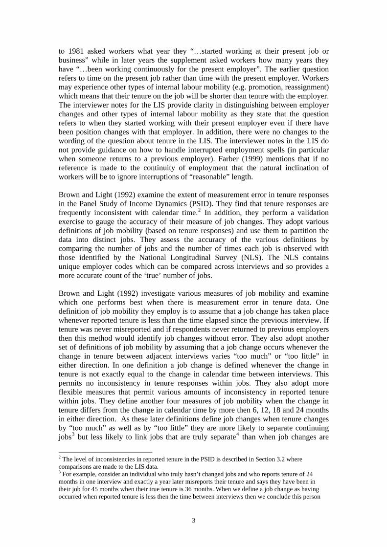
starting dates would be constant within jobs. By partitioning the dataset into distinct jobs and comparing starting dates across interviews we can investigate how consistent the data is. Table 1 shows the number of workers employed in consecutive two-year periods from the revolving balanced panel and the number of job changes each year. Table 1: Number of Workers and Job Changes 1995 1996 1997 1998 1999 2000 2001

Number of workers 1,185 1,229 1,274 1,337 1,406 1,449 1,497

No. Job Changes 77 89 110 146 151 195 159

To convert this data into separate jobs, we begin with the 1995 data. There are 1,185 workers in 1995 but as 77 workers changed jobs a total of 1,262 distinct jobs are observable in that year. For this year alone, the previous jobs of those who changed jobs are excluded from the analysis. We only have one observation on their previous jobs (the starting date in 1994) so we cannot check the consistency of responses whereas we can track the new jobs across subsequent interviews. Therefore, we start the analysis with 1,185 distinct jobs in 1995. In each subsequent year one of four alternatives occurs:

1) A worker can stay in their job so the total number of jobs remains the same and we observe the job surviving an additional year.

2) A worker can drop out of the sample if they enter a period of unemployment, leave the labour force for more than a year or if they are over the age of 60. In this case, the total number of jobs remains the same but we no longer observe that particular job. Workers who are unemployed or leave the labour force may re-enter the analysis in later years.

3) A worker can change jobs and accordingly the total number of jobs increases by one and we stop observing the previous job.

4) There can be a new entrant to the sample of workers. This would be someone from the revolving balanced panel who is now 20 and so was excluded in earlier years. This increases the total number of jobs by one. In addition, a worker who was unemployed or out of the labour force may come back into the analysis and this would increase the total number of jobs observed by one.

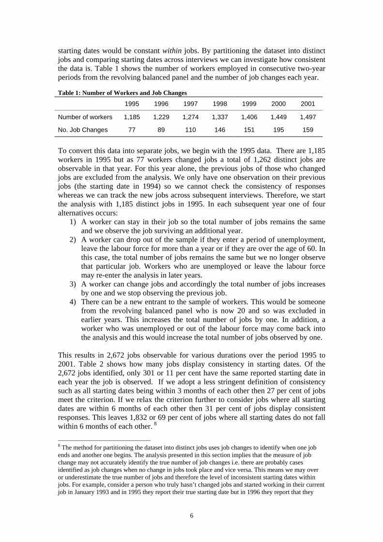
This results in 2,672 jobs observable for various durations over the period 1995 to 2001. Table 2 shows how many jobs display consistency in starting dates. Of the 2,672 jobs identified, only 301 or 11 per cent have the same reported starting date in each year the job is observed. If we adopt a less stringent definition of consistency such as all starting dates being within 3 months of each other then 27 per cent of jobs meet the criterion. If we relax the criterion further to consider jobs where all starting dates are within 6 months of each other then 31 per cent of jobs display consistent responses. This leaves 1,832 or 69 per cent of jobs where all starting dates do not fall within 6 months of each other. 8

8 The method for partitioning the dataset into distinct jobs uses job changes to identify when one job ends and another one begins. The analysis presented in this section implies that the measure of job change may not accurately identify the true number of job changes i.e. there are probably cases identified as job changes when no change in jobs took place and vice versa. This means we may over or underestimate the true number of jobs and therefore the level of inconsistent starting dates within jobs. For example, consider a person who truly hasn’t changed jobs and started working in their current job in January 1993 and in 1995 they report their true starting date but in 1996 they report that they

6

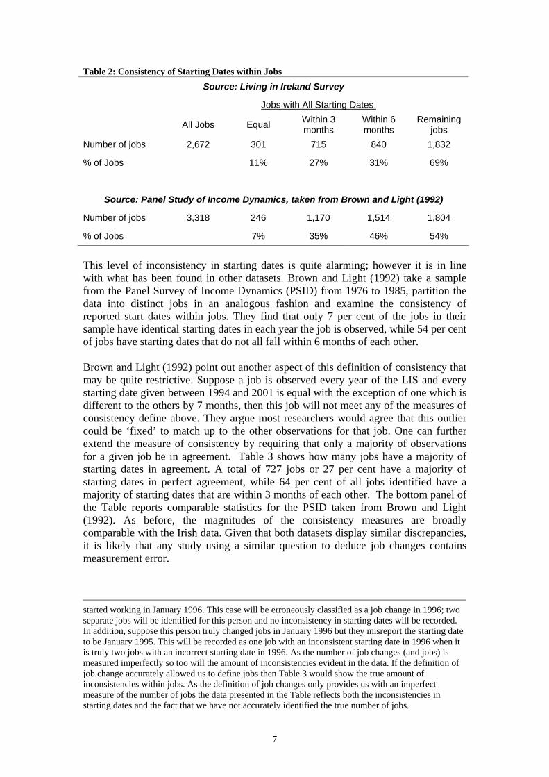
Table 2: Consistency of Starting Dates within Jobs

Source: Living in Ireland Survey

Jobs with All Starting Dates

All Jobs Equal Within 3 months

Within 6 months

Remaining jobs

Number of jobs 2,672 301 715 840 1,832

% of Jobs 11% 27% 31% 69%

Source: Panel Study of Income Dynamics, taken from Brown and Light (1992)

Number of jobs 3,318 246 1,170 1,514 1,804

% of Jobs 7% 35% 46% 54%

This level of inconsistency in starting dates is quite alarming; however it is in line with what has been found in other datasets. Brown and Light (1992) take a sample from the Panel Survey of Income Dynamics (PSID) from 1976 to 1985, partition the data into distinct jobs in an analogous fashion and examine the consistency of reported start dates within jobs. They find that only 7 per cent of the jobs in their sample have identical starting dates in each year the job is observed, while 54 per cent of jobs have starting dates that do not all fall within 6 months of each other. Brown and Light (1992) point out another aspect of this definition of consistency that may be quite restrictive. Suppose a job is observed every year of the LIS and every starting date given between 1994 and 2001 is equal with the exception of one which is different to the others by 7 months, then this job will not meet any of the measures of consistency define above. They argue most researchers would agree that this outlier could be ‘fixed’ to match up to the other observations for that job. One can further extend the measure of consistency by requiring that only a majority of observations for a given job be in agreement. Table 3 shows how many jobs have a majority of starting dates in agreement. A total of 727 jobs or 27 per cent have a majority of starting dates in perfect agreement, while 64 per cent of all jobs identified have a majority of starting dates that are within 3 months of each other. The bottom panel of the Table reports comparable statistics for the PSID taken from Brown and Light (1992). As before, the magnitudes of the consistency measures are broadly comparable with the Irish data. Given that both datasets display similar discrepancies, it is likely that any study using a similar question to deduce job changes contains measurement error.

started working in January 1996. This case will be erroneously classified as a job change in 1996; two separate jobs will be identified for this person and no inconsistency in starting dates will be recorded. In addition, suppose this person truly changed jobs in January 1996 but they misreport the starting date to be January 1995. This will be recorded as one job with an inconsistent starting date in 1996 when it is truly two jobs with an incorrect starting date in 1996. As the number of job changes (and jobs) is measured imperfectly so too will the amount of inconsistencies evident in the data. If the definition of job change accurately allowed us to define jobs then Table 3 would show the true amount of inconsistencies within jobs. As the definition of job changes only provides us with an imperfect measure of the number of jobs the data presented in the Table reflects both the inconsistencies in starting dates and the fact that we have not accurately identified the true number of jobs.

7

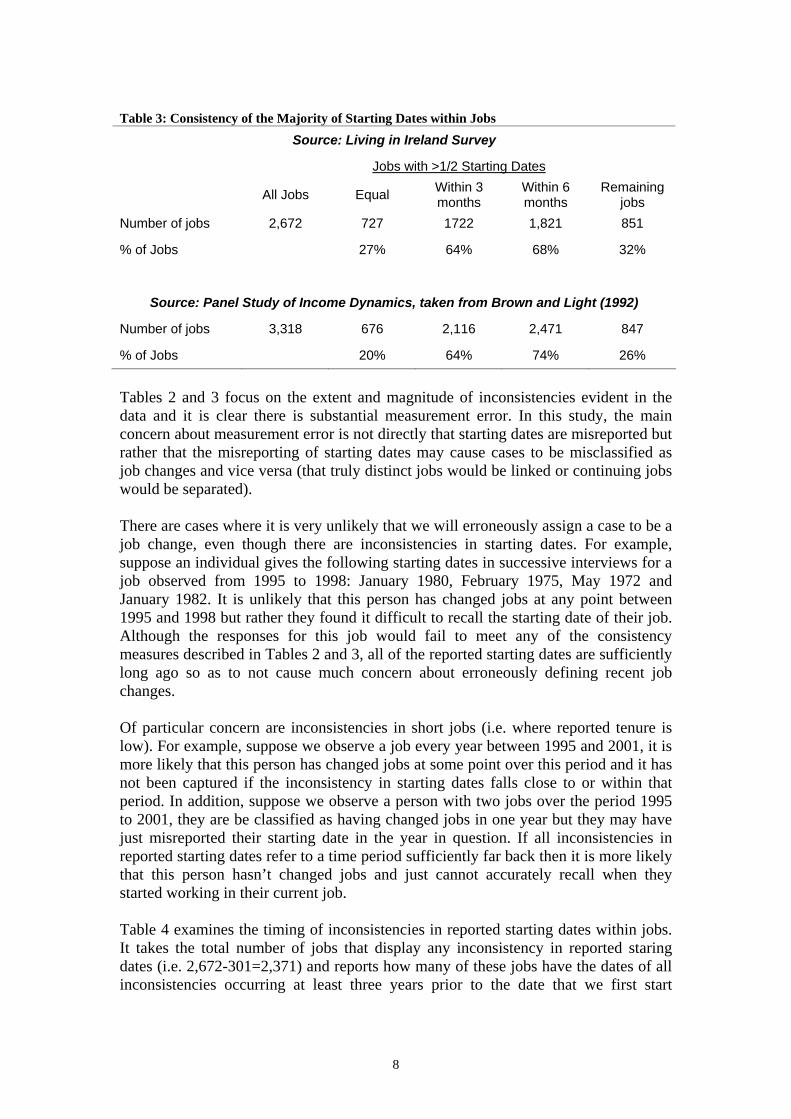
Table 3: Consistency of the Majority of Starting Dates within Jobs

Source: Living in Ireland Survey

Jobs with >1/2 Starting Dates

All Jobs Equal Within 3 months

Within 6 months

Remaining jobs

Number of jobs 2,672 727 1722 1,821 851

% of Jobs 27% 64% 68% 32%

Source: Panel Study of Income Dynamics, taken from Brown and Light (1992)

Number of jobs 3,318 676 2,116 2,471 847

% of Jobs 20% 64% 74% 26%

Tables 2 and 3 focus on the extent and magnitude of inconsistencies evident in the data and it is clear there is substantial measurement error. In this study, the main concern about measurement error is not directly that starting dates are misreported but rather that the misreporting of starting dates may cause cases to be misclassified as job changes and vice versa (that truly distinct jobs would be linked or continuing jobs would be separated). There are cases where it is very unlikely that we will erroneously assign a case to be a job change, even though there are inconsistencies in starting dates. For example, suppose an individual gives the following starting dates in successive interviews for a job observed from 1995 to 1998: January 1980, February 1975, May 1972 and January 1982. It is unlikely that this person has changed jobs at any point between 1995 and 1998 but rather they found it difficult to recall the starting date of their job. Although the responses for this job would fail to meet any of the consistency measures described in Tables 2 and 3, all of the reported starting dates are sufficiently long ago so as to not cause much concern about erroneously defining recent job changes. Of particular concern are inconsistencies in short jobs (i.e. where reported tenure is low). For example, suppose we observe a job every year between 1995 and 2001, it is more likely that this person has changed jobs at some point over this period and it has not been captured if the inconsistency in starting dates falls close to or within that period. In addition, suppose we observe a person with two jobs over the period 1995 to 2001, they are be classified as having changed jobs in one year but they may have just misreported their starting date in the year in question. If all inconsistencies in reported starting dates refer to a time period sufficiently far back then it is more likely that this person hasn’t changed jobs and just cannot accurately recall when they started working in their current job. Table 4 examines the timing of inconsistencies in reported starting dates within jobs. It takes the total number of jobs that display any inconsistency in reported staring dates (i.e. 2,672-301=2,371) and reports how many of these jobs have the dates of all inconsistencies occurring at least three years prior to the date that we first start

8

observing the job.9 There are 852 jobs where all discrepancies fall reasonably far in the past that so that these are probably truly continuing jobs. However, there are 1,519 jobs where the reported inconsistencies are more recent and it is more likely in these cases that we have linked jobs that are distinct or divided continuing jobs. Table 4: Timing of Inconsistencies within Jobs

Total No. Jobs

Equal Starting Dates

All inconsistencies at least 3 years prior to date job is first

observed

Remaining jobs

Number of jobs 2,672 301 852 1,519

% of Jobs 11% 32% 57%

If the true number of jobs has been under or overestimated (and therefore the true number of job changes has been under or overestimated), it may be more likely to do so for certain types of worker. As mentioned above, I am more likely to under or overestimate the number of jobs where reported inconsistencies are recent (i.e. jobs that report inconsistent short tenures). As tenure and years of work experience are correlated we may expect to see differences in inconsistencies in starting dates by years of experience. There may also be differences by gender; as women experience more interrupted employment spells than men it may be harder for them to accurately report starting dates. There are 1,519 jobs (from Table 4) that exhibit some type of inconsistency in starting dates within jobs where the dates associated with any inconsistency are relatively recent. Table 5 examines these jobs by years of work experience and gender. I have labelled these jobs as being ‘problematic’ in the sense that it is more likely that that truly distinct jobs would be linked or continuing jobs would be separated (i.e. that job changes are misclassified and vice versa). This is not to say that workers in short jobs are more likely to be misreport when they started working in their job than workers in long jobs, but rather that the misreporting by those in short jobs is more likely to lead to misclassifying cases as job changes and vice versa. The Table shows that the incidence of problematic jobs declines with years of work experience.10 For example, 76 per cent of jobs that have less then ten years of work experience associated with them are classified as problematic and this percentage declines as years of experience increases so that only 31 per cent of jobs with more then 30 years of work experience associated with them fall into this category. As there are more of these problematic jobs in low experience categories and job mobility is negatively correlated with experience, this may indicate that we are underestimating the true number of job changes. There is also some difference when we look at the incidence of these problematic jobs by gender; 53 per cent of all jobs held by men fall into this category while the

9 For example, if we observe for the first time in 1995 this measure counts all jobs where each inconsistency refers to dates earlier then or in 1992. 10 In assigning years of work experience to a worker in a job we use their experience in the first year that the job is observed. For example, if we observe a job each year between 1995 and 2001 the experience assigned to that job when comparing all combinations of starting dates over the period is the years of experience of that person is in 1995.

9

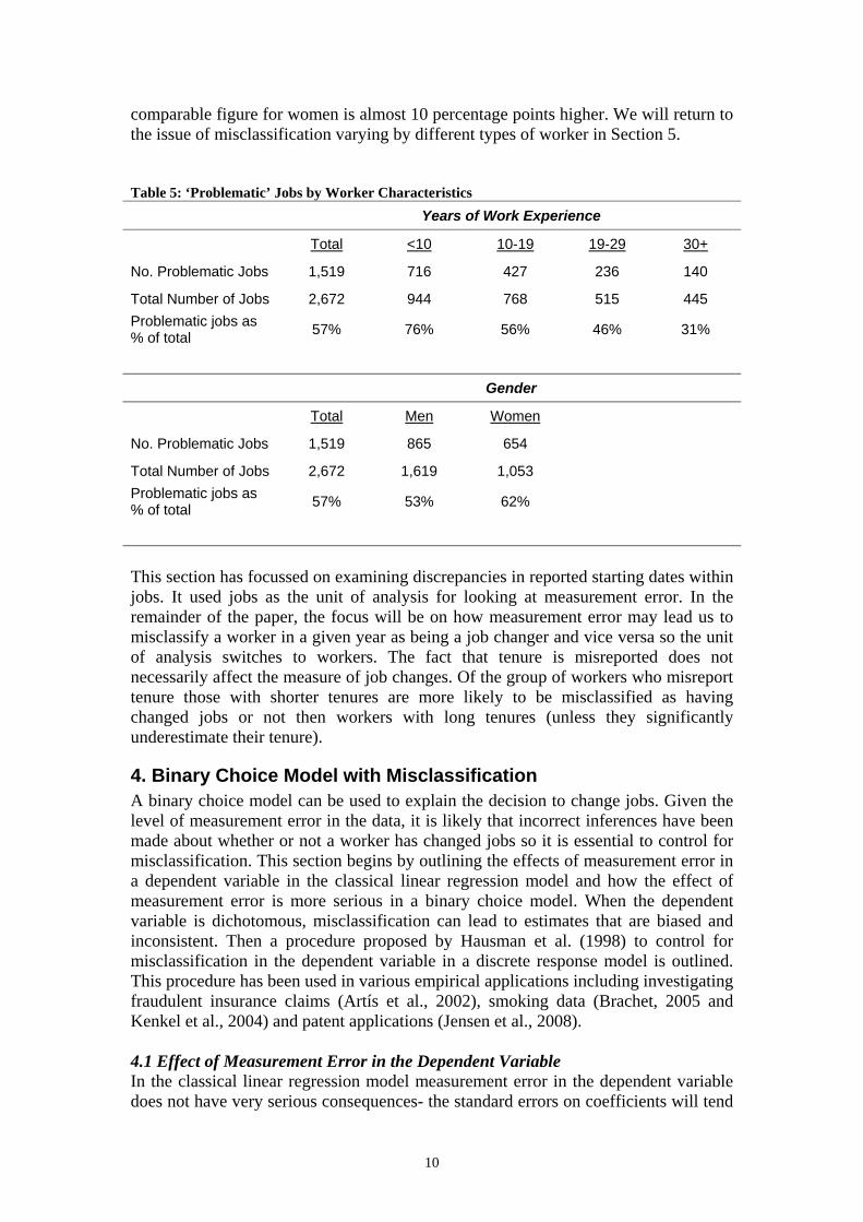
comparable figure for women is almost 10 percentage points higher. We will return to the issue of misclassification varying by different types of worker in Section 5. Table 5: ‘Problematic’ Jobs by Worker Characteristics Years of Work Experience Total <10 10-19 19-29 30+

No. Problematic Jobs 1,519 716 427 236 140

Total Number of Jobs 2,672 944 768 515 445 Problematic jobs as % of total 57% 76% 56% 46% 31%

Gender Total Men Women

No. Problematic Jobs 1,519 865 654

Total Number of Jobs 2,672 1,619 1,053 Problematic jobs as % of total 57% 53% 62%

This section has focussed on examining discrepancies in reported starting dates within jobs. It used jobs as the unit of analysis for looking at measurement error. In the remainder of the paper, the focus will be on how measurement error may lead us to misclassify a worker in a given year as being a job changer and vice versa so the unit of analysis switches to workers. The fact that tenure is misreported does not necessarily affect the measure of job changes. Of the group of workers who misreport tenure those with shorter tenures are more likely to be misclassified as having changed jobs or not then workers with long tenures (unless they significantly underestimate their tenure).

4. Binary Choice Model with Misclassification A binary choice model can be used to explain the decision to change jobs. Given the level of measurement error in the data, it is likely that incorrect inferences have been made about whether or not a worker has changed jobs so it is essential to control for misclassification. This section begins by outlining the effects of measurement error in a dependent variable in the classical linear regression model and how the effect of measurement error is more serious in a binary choice model. When the dependent variable is dichotomous, misclassification can lead to estimates that are biased and inconsistent. Then a procedure proposed by Hausman et al. (1998) to control for misclassification in the dependent variable in a discrete response model is outlined. This procedure has been used in various empirical applications including investigating fraudulent insurance claims (Artís et al., 2002), smoking data (Brachet, 2005 and Kenkel et al., 2004) and patent applications (Jensen et al., 2008). 4.1 Effect of Measurement Error in the Dependent Variable In the classical linear regression model measurement error in the dependent variable does not have very serious consequences- the standard errors on coefficients will tend

10

to be larger then they would have been if there were no measurement error. Consider the following model:11 iii xy εβ +=~ i=1,……n where n is sample size, iε is i.i.d and all variables are measured as deviations

from sample means Suppose that iy~ is the true dependent variable but that it is measured with error so what we actually observe is: iii vyy += ~ where is assumed to be independent of the covariates and iv iε so iii xy ωβ += where iii v+= εω The effect of measurement error in is an error term with increased variance since the new error term,

iy

iω , contains both the original error term, iε , and the measurement error, . In this case, the OLS estimates of iv β will remain unbiased but will be measured with less precision. In a non-linear regression model, such as a probit model, the effects of measurement error are more severe. If the dependent variable is binary, measurement error takes the form of misclassification errors; some observations where the variable is truly a 1 will be misclassified as a 0 and vice versa. In this case, if the true value is 1(0) but it is misclassified as a 0(1) then the measurement error (observed minus true value of dependent variable) will be negative (positive). In this case the measurement error is negatively correlated with the true variable. This can lead to coefficient estimates that are biased and inconsistent. 4.2 Standard Model of Misclassification The decision to change jobs can be set in the usual latent-variable specification of the binary choice model. The Hausman et al. (1998) model of misclassification can be used for this application as follows:12 Let be the latent variable that represents the potential or tendency for a worker to change jobs. is a continuous variable that is unobservable and is determined by a set of explanatory variables, , in such a way that the larger the value of , the greater the probability of changing jobs.

iy*

iy*

ix iy*

where i=1, 2 …n n = sample size (1) iii xy εβ += '*

and iε is an independently and identically distributed error term. We cannot observe the tendency for a worker to change jobs; instead in the usual binary choice model we observe whether a worker changes jobs or not so for each worker there is a threshold or critical level, , at or above which they change jobs otherwise they stay in their iy*

11 Hausman (2001) discusses the effects of measurement error in dependent variables. 12 The details of the model come from Hausman et al. (1998).

11

jobs. The true response (or what we would observe in the data if there was no measurement error), iy~ , is given by:

1~ =iy if (2) 0* ≥iy =0 otherwise.

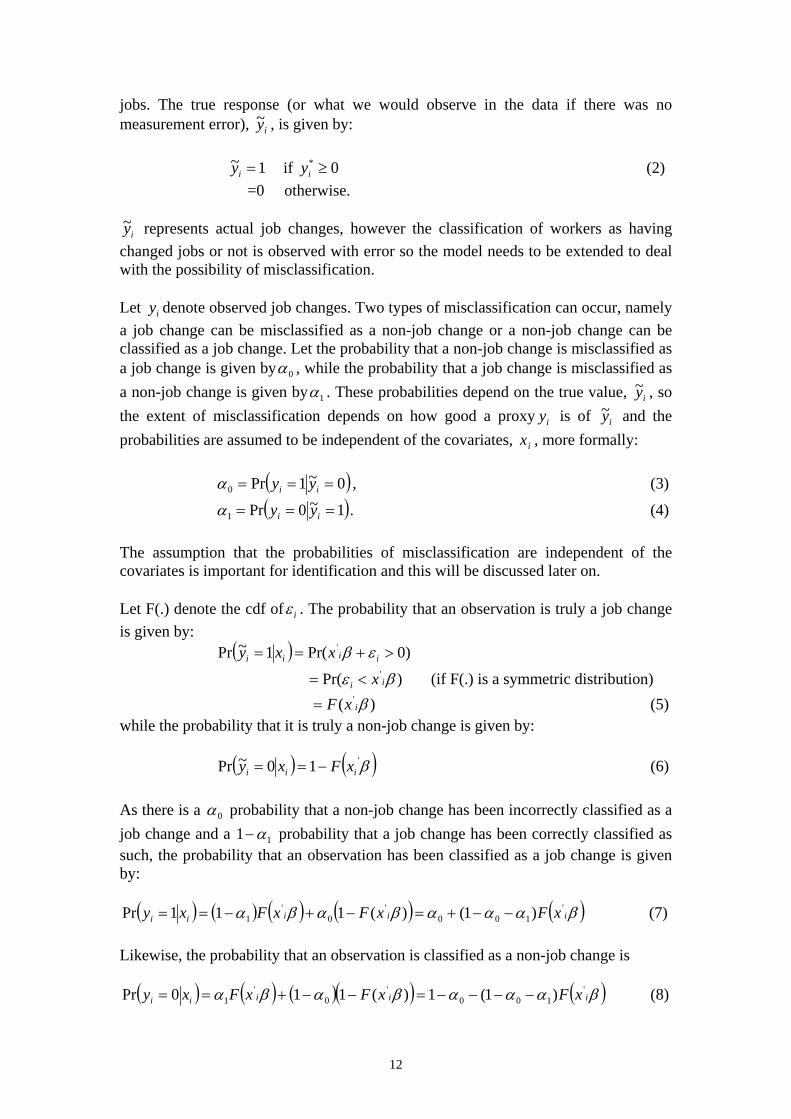
iy~ represents actual job changes, however the classification of workers as having changed jobs or not is observed with error so the model needs to be extended to deal with the possibility of misclassification. Let denote observed job changes. Two types of misclassification can occur, namely a job change can be misclassified as a non-job change or a non-job change can be classified as a job change. Let the probability that a non-job change is misclassified as a job change is given by

iy

0α , while the probability that a job change is misclassified as a non-job change is given by 1α . These probabilities depend on the true value, iy~ , so the extent of misclassification depends on how good a proxy is of iy iy~ and the probabilities are assumed to be independent of the covariates, , more formally: ix

( )0~1Pr0 === ii yyα , (3)

( )1~0Pr y1 === ii yα . (4)

The assumption that the probabilities of misclassification are independent of the covariates is important for identification and this will be discussed later on. Let F(.) denote the cdf of iε . The probability that an observation is truly a job change is given by: ( ) )0Pr(~ 1Pr ' >+= iiii xxy εβ

)

=

(if F(.) is a symmetric distribution) )Pr( ' βε ii x<=

(5) ( ' βixF=while the probability that it is truly a non-job change is given by:

( ) ( )β'1~ 0Pr iii xFxy −== (6)

As there is a 0α probability that a non-job change has been incorrectly classified as a job change and a 1 1α− probability that a job change has been correctly classified as such, the probability that an observation has been classified as a job change is given by:

( ) ( ) ( ) ( ) ( )βαααβαβα iiiii xFxFxxy '100

'0

'1 )1()(111Pr −−+=−+−== F (7)

Likewise, the probability that an observation is classified as a non-job change is

( ) ( ) ( )( ) ( )βαααβαβα iiiii xFxFxFxy '100

'0

'1 )1(1)(110Pr −−−−=−−+== (8)

12

The expected value of the observed dependent variable is given by: iy ( ) ( )βααα iiiii xFxyxyE '

100 )1()1Pr( −−+=== (9) When there is no misclassification ( )010 ==αα , this collapses to usual expression . )( ' βixF If we assume that iε are normally distributed then we can use equations (7) and (8) to derive the log-likelihood function for the probit model with misclassification:

( )( ) ( ) ( )( ){ }∑=

==−+==n

iiiiiii xyyxyyL

10Prln11Prlnln

( ) ( )( ) ( ) ( ) ( )( ){ }∑=

Φ−−−−−+Φ−−+n

iiiii xyxy

1

'100

'100 11ln11ln βαααβααα (10)

where ( ).Φ denotes the cdf of the normal distribution Maximising the log-likelihood function given in (10) with respect to 10 ,αα and β yields consistent and efficient estimates of β as well as the probabilities of misclassification. Identification The conditions for identification of 10 ,αα and β are similar to those for the traditional binary choice model. One additional assumption is needed for identification, namely that the misclassification probabilities are not very large, specifically, 110 <+αα . This assumption is needed because the normal distribution is symmetric ( =1- ) and we can define)( ' βixΦ )( ' βix−Φ 10 1 αα −= , 01 1 αα −= and

ββ −= so that:

( )( )( )( ) )'()1()'(1)(1()1(

'(1)1()1(1)1()'()1(

100101

011100

βαααβαααβαααβααα

ii

ii

xxxx

Φ−−+=Φ−++−+−=−Φ−−−−−+−=Φ−−+

(11)

When the assumption, 110 <+αα , is not imposed the maximum likelihood estimator cannot distinguish between the parameter values ),,( 10 βαα and ),1,1( 10 βαα −−− . The assumption that 110 <+αα excludes this situation because 110 <+αα implies 1)0 >1()1( 1 −+− αα . An implication of this assumption is that if 110 >+αα but we impose 11 <0 +αα the estimates of β will have the wrong sign. This assumption guarantees that ( )βαα 10 )Φ−α0 1(+ ix '− is strictly increasing in as

(.) is strictly increasing. βix '

Φ

13

The model parameters are identified from the nonlinearity of ( ).Φ . To see this consider the linear probability mod )'( βix= , then the expected value of iy is giv

el wheren by:

e )( ' βixF

( ) ( )

))1(()(

)1()1Pr(

110'

00

'100

βααβα

βααα

−−++=

−−+===

i

iiiii

z

xxyxyE (12)

where and (i.e. separating out the constant)

'' ),1( ii zx = '1'

0 ),( βββ =

In this case the parameters of the model cannot be separately identified. Estimating 0α and 1α is only possible because they enter (10) additively and are then multiplied by the expression with the normal cdf. This can be seen more clearly by taking limits of ( )ii xyE as tends to βix ' ∞− and ∞+ in (9).

0)(lim'

αβ

=Ε−∞→

iix

xyi

and 11)(lim'

αβ

−=Ε∞→

iix

xyi

(13)

To identify the misclassification probabilities, 0α and 1α , has to get reasonably large in magnitude so as to push

βix '

( )ii xy 1~Pr = close to 0 and 1 for some i. The intuition behind this is that we have assumed that misclassification rates are constant and depend only on the true value, iy~ , so the probability of misclassifying a non-job change as a job change, 0α , is identified from the group of workers with a near zero probability of truly changing jobs. These are workers for whom is highly negative and who are therefore very unlikely to be job changers. Hconstant proportion,

βix '

owever, as a 0α , are misclassified as having changed jobs, ( )iiyPr = x1 will

never fall below 0α regardless of how negative is. In a similar fashion, the probability of misclassifying a job change as a non-job change, 1

βix '

α , is estimated from the group of workers for whom is very large and so have a very high probability of truly changing jobs but may be misclassified as not having changed jobs. Therefore

βix '

( ii xy 1Pr = ) will never rise above 11 α− . Marginal Effects From equation (5) we know that the expected value on the true response, iy~ , is given by:

( ) ( )β')1~Pr(~

iiiii xFxyxyE === (14) In general, we are usually more interested in the marginal effect of a specific variable, k, which is given by:

( ) ( ) kiik

ii

ik

ii xfx

xyx

xyEββ'

)1~Pr(~=

∂=∂

=∂

∂ (15)

14

Equation (9) gives the expected value on the observed response, , and the marginal ffect of a variable, k, is:

iye

( ) ( ) ( ) kiik

ii

ik

ii xfx

xyx

xyEββαα '

101)1Pr(

−−=∂=∂

=∂

∂ (16)

the margina

Comparing equations (15) and (16) shows that when there is misclassification error

l effects of interest (from equation (16)) will be biased towards zero (as ( )101 αα −− < 1). The marginal effects on the observed response will always be less then the marginal effects on the true response by a factor of ( )101 αα −− . This result nly holds when misclassification is independent of the covariates.

is

o To see the intuition behind this result, consider the following simple example: suppose you have a sample of 20 people, 10 of whom have a high value of some characteristic that makes them more likely to change jobs and the remaining 10 people have a low value of this characteristic that makes them less likely to change jobs. Further suppose that 8 people from the first group and 4 from the second group are identified as job changers. Then the true marginal effect on the characteristic is 0.4 (0.8-0.4). Now further suppose that we introduce misclassification (that does not depend on the particular characteristic) such that 4 out of the 8 true non job changes are m classified (i.e. 0α =.5) and 3 out of the 12 true job changes are misclassified (i.e. 1α =.25). As the misclassification probabilities are assumed not to depend on the characteristic, this implies that 1 job stayer from the first group and 3 from the second group are misclassified as job changers and 2 job changers from the first group and 1 from the second group are misclassified as job stayers. Then the marginal effect on the characteristic is 0. 7-0.6) which is a quarter or1 (0. ( )101 αα −− of the true marginal effect.

o the model to llow for some covariate dependent misclassification error as follows:

a he misclassification probabilities depends on some or all of the ovariates :

5. Covariate-Dependent Misclassification The analysis in Section 4 focussed on the case where misclassification is independent of the covariates or where the probabilities of misclassification are constant across all workers. Assuming that the probabilities of misclassification are constant across all types of workers may be quite restrictive. As indicated in Section 3.2 (in particular in Table 5) it is likely that the probabilities of misclassification vary across different types of workers. Hausman et al. (1998) consider a simple extension ta Assume th t t

ixc ( ) ( )iiii xyyx ,0~1Pr0 ===α (17)

( ) ( )iiii xyyx ,1~0Pr1 ===α (18)

he expected value of the observed dependent variable is:

T

15

( ) ( ) ( ) ( )( ) ( )βααα iiiiiiii 100

For example, suppose misclassific

xFxxxxyxy '1()1Pr( −−+=== (19)

ation only depends on one covariate , then the xpression given in (19) becomes:

E

1ixe

( ) ( ) ( ) ( )( ) ( )βααα iiiiiiii 111010

and the likelihood function is similar to equation (10) only the two misclassification probabilities appear as a function of 1ix . The model can be identified in a similar manner o what was described

xFxxxxyxy '1()1Pr( −−+=== (20)

t in Se n 4.2. To see this, first consider the case here is a dummy variable:

E

ctio 1xw i

1100 xγγα += (21)

1101 x∂+∂=α (22) and

11 =x ⇒ and Therefore when 100 γγα += 101 ∂+∂=α and when

(23) 0 001 γα =⇒=x and 01 ∂=α (24)

he expected value of the observed dependent variable becomes:

T

( ) ( ) ( ) ( )βδγγγγ iiiii 110110110

The identificatio e misclassification p babilities can be seen e clea by taking

xFxxxxyxy ')1()1Pr( ∂+−+−++=== (25)

n of th ro mor rly limits of

E

( )ii xyE as (where excludes ) tends to and in 5):

βix ' βix '1ix ∞− ∞+

(2

0)(lim'

γβ

=Ε−∞→

ii xyi

when and 01 =ix 10)(lim'

γγβ

+=Ε−∞→

iix

xyix

when (26)

11 =ix

)1()(lim 0'δ

β−=Ε

∞→ii

xxy

i

when 01 =ix and )1()(lim 10'δδ

β−−=Ε

∞→i

xy

i

when 11 =ix (27)

Intuitively if misclassification depends on 1ix , then the babiliti f misclassification are constant within the two subgroups where 11 =ix and 01 =ix . Then 0

ix

pro es o

γ is identified from the grou orkers w truly have a very low probability of changing jobs and who have 01

p of w ho=ix , while 1γ is identified from the gro f

workers who truly have a very low probability of changing jobs and who have 1ix . Similar to before, identification is achieved from the group of workers for whom βix ' is highly negative and who are therefore very unlikely to be job changers but some of them will be misclassified only i case we effectively divide this group of workers into two subgroups where 11

up o1=

n this=ix and 01 =ix . A comparable argument can be

made for the identification of 0δ and 1δ . Whe a dummy var hersclassif

n x 1i is iable t e are four mi ication probabilities to estimate.

16

If 1ix is a discrete variable, then all observations within the subgroups that have the same values for 1ix will have const isclassifica robabilities and identification is achieved in a similar way as described above. However, if we ha e many subgroups it will harder to estimate 210 ,,

ant m tion pv

γγγ etc and 210 ,, δδδ etc as there may not be s nt workers in the tails of the index with the full range of values of 1ix . Finally, if 1ix is a co

ufficienuous variable, we ne cut-o

only possible because the misclassification probabilities ess then one.

n es. The explanatory variables

at ch

nti can defi ff points 321 ,, ccc etc such that if 11 cxi < the misclassification probabilities are constant (or almost constant) within each group. As before, identification is enter the likelihood function in an additive way and their sum must be l

6. Estimation Results 6.1 Estimation Results: Misclassification Independent of Covariates Table 7 shows the estimates from a standard probit regression of the probability of job change and the estimates from the Hausman et al. procedure to control for misclassification. This provides estimates of the probabilities of misclassification and allows comparisons to be made on the effect of response error on the estimated coefficients. The data for 1995 to 2001 have been pooled so that there are 9,377 bservations from which I have identified 927 job cha go

are defined in Table A1. Zero misclassification probabilities are used as starting values in estimating the model with misclassification.13 The estim ed probability of misclassification for non-job angers, 0α is very small at less than one per cent and the estimated probability of misclassification for job changers, 1α , is high at 54 per cent. Significance tests on 0α and 1α can be used as tests of misclassification. Although 0α is not sig ificant, 1n α is highly significant and so we reject the model without misclassification. Workers who have truly changed jobs are more likely to be misclassified, as 1α exceeds 0α . This means that the measure of job change is likely to undercount the true number of job changes. Hausman et al. also apply the procedure to a model of job change using data from the January 1987 Curren Population Survey frt om the Census Bureau. Their study rovides an external estimate of the misclassification probabilities. They estimate p 0α

to be 6.1 per cent and 1α to be 30.9 per cent.

13 A range of different starting values for 0α and 1α were used to check the robustness of the results.

If 0α is given a starting value of 0, the results are robust for any starting value of 1α between 0 and 1.

Similarly if 1α is given a starting value of 0, the results are robust for any starting value of 0α

between zero and 1. If 0α and 1α are given the same starting values, the results are robust up to starting values of 0.32. For starting values between 0.32 and 0.45 the iterations don’t make any progress. For higher starting values such as 0.46 the program estimates ),,1( 10 1 βαα −−− and for starting values around 0.6 the results are not sensible.

17

When we allow for misclassification, the estimated coefficients have higher standard errors implying that errors in responses lead to a loss in estimation efficiency. The esults also indicate that ignoring response misclassification leads to diminished

s in estimates from the two regress ns if we look at m ect of c stim se are

in Table 8.

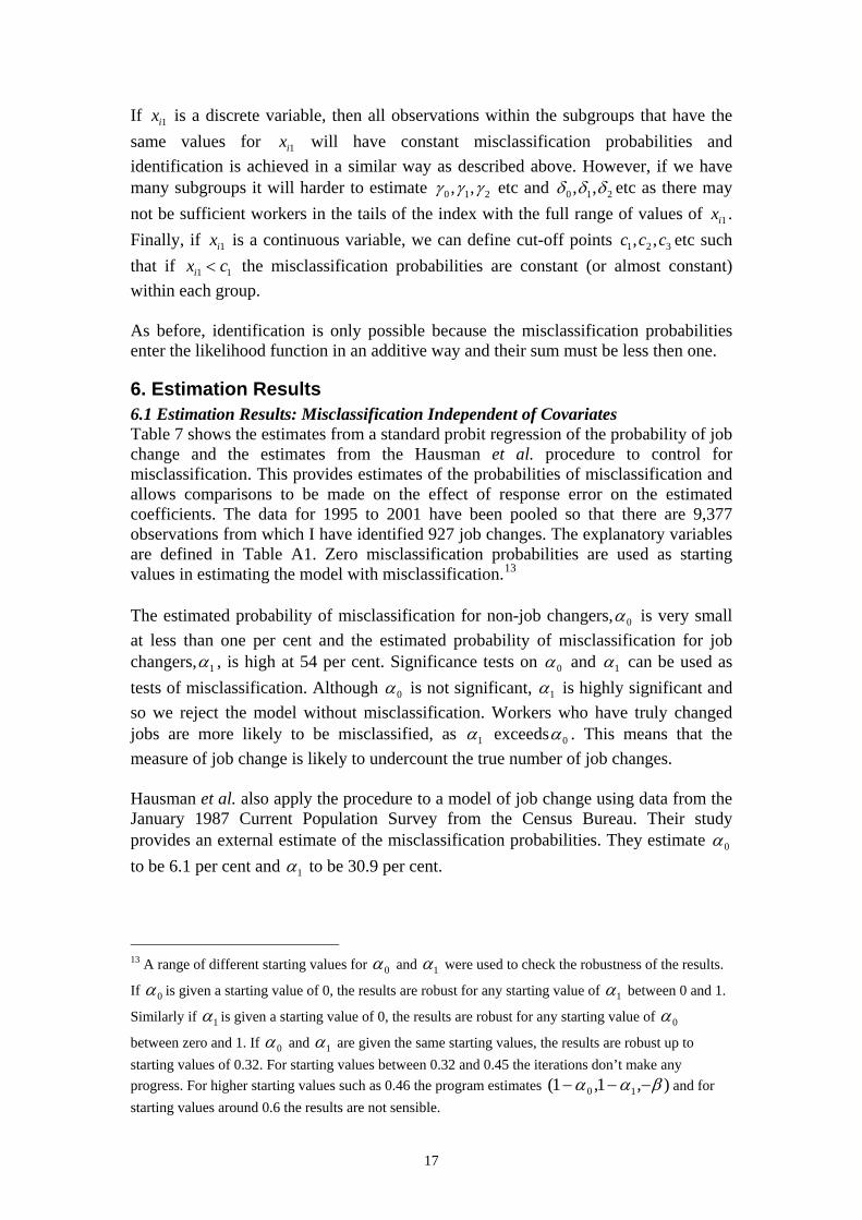
Ta le 7: Coefficient Estimates from odels of Job Change*^

Coefficient E

Standard C t E

Standard

rcovariate effects. It is easier to interpret difference

iopresented

arginal eff s instead oefficient e ates. The

b M

Variable stimate Errors oefficienstimate Errors

Standard Probit Model ification Misclass Model

0α 0.0091 0.0089

1α 0.5407 0.1970 Experience -0.0 48 0.0078 -0.1187 0.0465

uared

-0.2068 0.0769 -0.2896 0.1312 loyees > 50

on of Origin: entary Occ’s)

-0.4953 0.0959 -0.7898 0.3591

rvices) & Utilities -0.3759 0.1156 -0.5935 0.3181

ring -0.2238 0.0985 -0.3733 0.2263 g t Services

mies: 5)

1999 0.2246 0.0765 0.3660 0.1872 0.3579 0.5995 0.2254 0.4004 -0.3 83 0.6 6

-2645.73

7Experience sq 0.0011 0.0002 0.0018 0.0008 Education- medium -0.1283 0.0551 -0.1914 0.1017 Education- high (Ref: Education – low)

-0.1745 0.0919 -0.3104 0.2003

Public Sector Number of EmpOverskilled

-0.1755 0.0498 -0.2847 0.1363 0.2095 0.0399 0.3192 0.1150

Occupati (Ref: Elem Manager Professional -0.3966

-0.3191 0.0817 0.0680

-0.5963 -0.5412

0.2276 0.2794 Clerk

Skilled -0.3412 0.0709 -0.5033 0.1757 Sector of Origin: (Ref: Non Market Se

Agric. & Mining Manufactu Buildin 0.3526 0.1098 0.5859 0.3041 Marke 0.1483 0.0780 0.2338 0.1513 Year Dum (Ref: 199 1996 0.0225 0.0767 0.0679 0.1301 1997 0.0893 0.0785 0.1733 0.1565 1998 0.2422 0.0734 0.4174 0.2309 2000 2001

0.0743 0.2828 0.0748 0.2331

Constant 5 0.1259 03 0.7951 N 9,377 9,377 Wald chi2 481.18 31.67 Prob > chi2 0.000 0.0632 og pseudolikelihood -2647.10 L

* Note: Standard errors are adjusted to take account of the facthe same people

t that there are multiple observations on

^ Note: Controls for gender, pr ildren ital s gion clude del d from the final speci cause ere n ant

esence of chfication be

, mar they w

tatus and reot signific

were in d in the mobut droppe

18

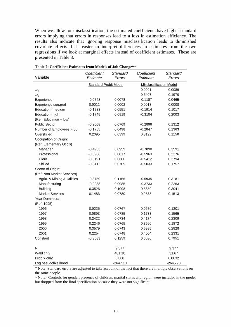
Ta le 8: Marginal Effects from M s of Job C ange*^

M M % diff. in M l E

b odel h

Variable arginalEffect P>|Z| arginal

Effect P>|Z|

arginaffects

Standard Probit l Mode ication ModelMisclassif

0α 0.0091 0.31

1α 0.5407 0.01

edium -0.0220 0.06 -0.0635 0.12 28

oyees > 50

d

-0.0512 0.00 -0.1271 0.03 24

t Services) ining & Utilities -0.0425 0.00 -0.1023 0.06 24

acturing g t Services

mies: 5)

1997 0.0130 0.26 0.0427 0.27 321998 0.0380 0.1114 29

0.0349 0.0959 270.0592 0.1677 280.0349 0.1057 30

rob > chi2 0.000 0.0632

Experience -0.0104 0.00 -0.0419 0.01 404% Experience squared 0.0002 0.00 0.0007 0.02 412% Education- m -0.0175 0.02 -0.0435 0.06 249% Education- high 8% (Ref: Education – low) Public Sector -0.0269 0.01 -0.0627 0.03 233% Number of Empl -0.0234 0.00 -0.0630 0.04 269% Overskille 0.0294 0.00 0.0747 0.01 254% Occupation of Origin: (Ref: Elementary Occ’s) Manager 8% Professional -0.0477 0.00 -0.1173 0.01 246% Clerk -0.0392 0.00 -0.1072 0.05 274% Skilled -0.0412 0.00 -0.0997 0.00 242% Sector of Origin: (Ref: Non Marke Agric. & M 1% Manuf -0.0280 0.02 -0.0762 0.10 272% Buildin 0.0602 0.00 0.1693 0.05 281% Marke 0.0212 0.06 0.0561 0.12 264% Year Dum (Ref: 199 1996 0.0032 0.77 0.0161 0.60 510% 9% 0.00 0.07 3% 1999 0.00 0.05 5% 2000 0.00 0.03 4% 2001 0.00 0.09 3% N 9,377 9,377 Wald chi2 481.18 31.67 PLog pseudolikelihood -2647.10 -2645.73 * Note: Standard errors are adjusted to take account of the fact that there are multiple observations on the same people ^ Note: Controls for gender, presence of children, marital status and region were included in the model but dropped from the final specification because they were not significant Although both models indicate that the same factors determine job mobility the effect of misclassification in the dependent variable on the marginal effects of the various explanatory variables is sizeable.14 In the theoretical literature on job mobility, years 14 The marginal effects are evaluated at the sample means of the explanatory variables.

19

of labour market experience is a key determinant of job change and both models provide findings that are consistent with this. However, in the model that does not llow for misclassification the marginal effect of an additional year of experience is to

in elementary occupations are higher in the isclassification model. Working in the public sector is found to exert a negative

al ffects are higher in the misclassification model. Finally, the marginal impacts of

flatten out at igher years of experience indicating that an additional year of experience reduces the

probability of changing jobs but at a declining rate (i.e. the marginal effect on years of experience squared is positive). Overall, the graph shows that the effect of ignoring misclassification error is large, especially at low values of experience.

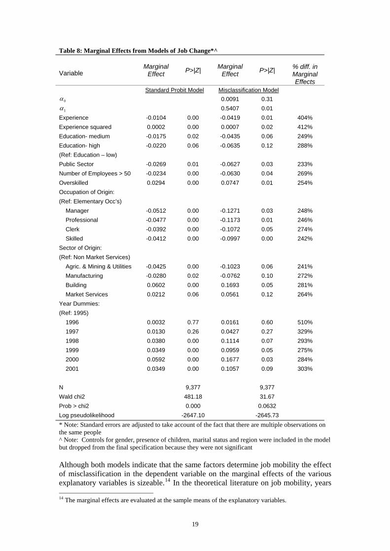
areduce the probability of changing jobs by 1 percentage point, while the marginal effect in the misclassification model is almost four times larger so an additional year of experience reduces the probability of changing jobs by 4.2 percentage points. The results also indicate that the negative effect of human capital on the probability of changing jobs is more marked in the misclassification model. For example, general human capital is proxied by education level and in the model incorporating misclassification the marginal effect of third level education almost three times higher then in the probit model, indicating that those with third level education are 6.4 per cent less likely to change jobs then those who have at most Junior Certificate education. The occupation indicator variable is intended to capture more specific human capital and again the marginal effects of higher levels of occupational attainment relative to those meffect on the probability of changing jobs and the marginal impact of working in the public sector in the misclassification model is over double the impact than in the model without misclassification. The effect of the sector a worker was in the previous year (or for job changers the sector they previously worked in) is similar in both models but again the marginebeing overskilled, an indicator of poor match quality, working in a firm with more then 50 employees and the time dummies, which capture factors that vary over time but that affect all people are all bigger in magnitude in the misclassification model. A useful way to demonstrate the differences between the two models is to graph the marginal effects of the variables. Figure 1 plots the marginal effect of experience from both models. The curves slope down as the probability of job change decreases as years of experience increases (i.e. the marginal effect on experience is negative). The slopes of the curves are steep at lower values of experience and thenh

20

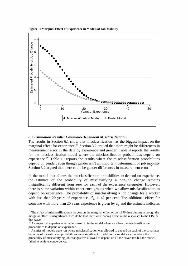
Figure 1: Marginal Effect of Experience in Models of Job Mobility

ation Results: Covariate-Dependent Misclassification

nt determinant of job mobility ection 3.2 argued that there could be gender differences in measurement error.17

ries. However, there is some variation within experience groups when we allow misclassification to depend on experience. The probability of misclassifying a job change for a worker with less then 20 years of experience,

.6.8

1

.2 Estim6The results in Section 6.1 show that misclassification has the biggest impact on the marginal effect for experience.15 Section 3.2 argued that there might be differences in measurement error in the data by experience and gender. Table 9 reports the results for the misclassification model where the misclassification probabilities depend on experience.16 Table 10 reports the results where the misclassification probabilities depend on gender; even though gender isn’t an importaS In the model that allows the misclassification probabilities to depend on experience, the estimate of the probability of misclassifying a non-job change remains insignificantly different from zero for each of the experience catego

0δ , is 42 per cent. The additional effect for someone with more than 20 years experience is given by 1δ and the estimate indicates 15 The effect of misclassification is largest on the marginal effect of the 1996 time dummy although the marginal effect is insignificant. It could be that there were coding errors in the responses to the LIS for that wave. 16 A categorical experience variable is used to in the model when we allow the misclassification probabilities to depend on experience. 17 A series of models were run where misclassification was allowed to depend on each of the covariates but none of the estimated probabilities were significant. In addition, a model was run where the probability of misclassifying job changes was allowed to depend on all the covariates but the model failed to achieve convergence.

0.2

.4

0 10 20 30 40 50Years of Experience

Misclassification Model Probit Model

Est

imat

ed P

roba

bilit

y of

Job

Cha

nge

21

that these workers are almost 37 percentage points less likely to be misclassified as not having changed jobs then someone with less then 20 years experience. Although

of the estimated probabilities are what we would expect none of the gnificant. In general, the coeff ates are similar

the model where misclassification is i dependent of the covariates. In addition, th imation efficiency as the standard errors are a little higher than b W tion probabilities depe nder, the obabilitym change is not statistically different from zero for me

omen. The probability of misclassifying a job change is around 54 per cent for men ditional effect of misclassifying a job change for wome all and not

more there is a small loss in ion efficien n we ion probabilities to differ by ge

the variation in the data is not sufficient to ely id sclassification or the results presented in Ta and 10

at misclassification is independent of the covariates.

the signsestimated probabilities are si icient estimto n

ere is some loss in estefore.

hen the misclassificaisclassifying a non-job

nd on ge pr of n and

wand the ad n is smsignificant. Once estimat cy whe allowthe misclassificat nder.

he caseIt may be t accurat entifycovariate dependent mi bles 9 may indicate th

22

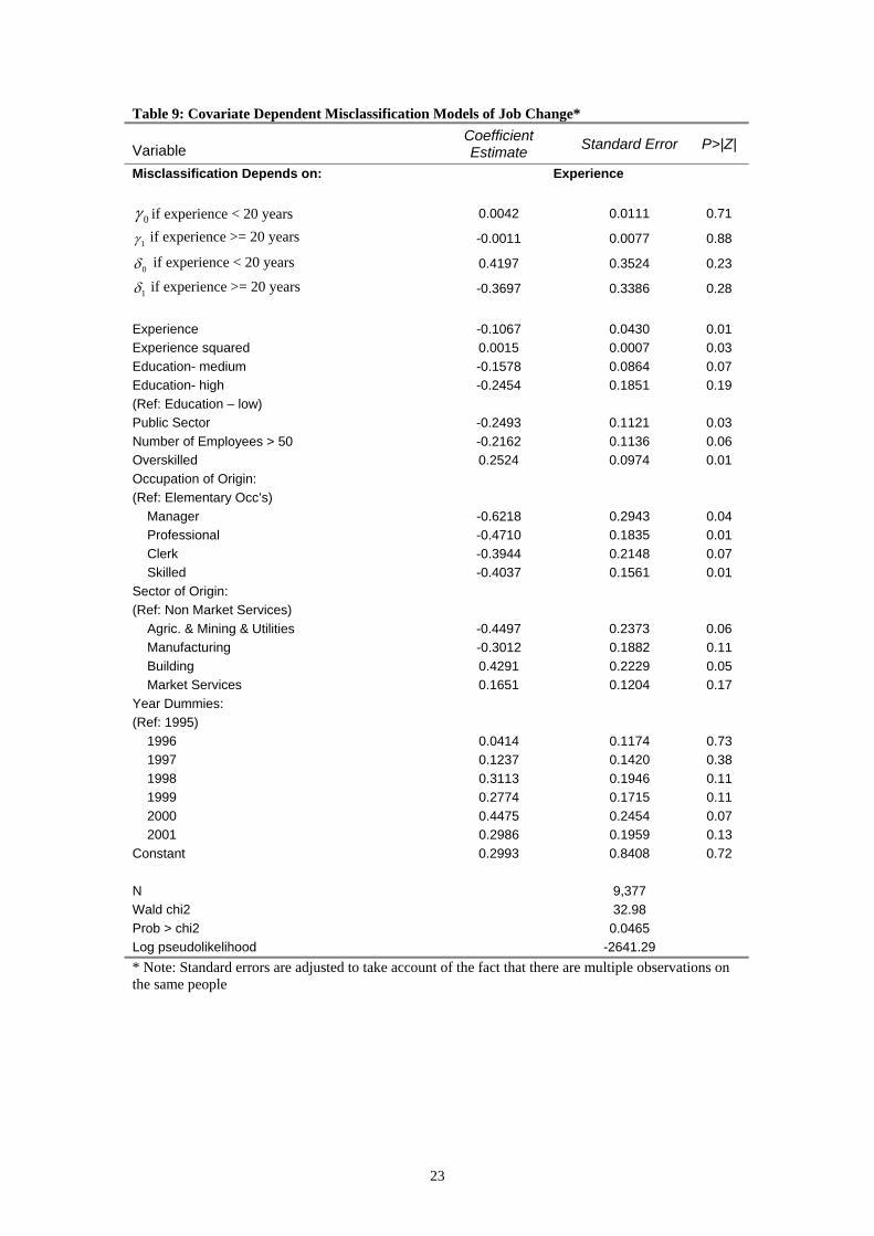
Table 9: Covariate Dependent Misclassification Models of Job Change*

Variable CoeEs

fftim d r P>|Z| icient

ate Stan ard Erro

Misclassification Depends on: Experience

0γ if experience < 20 years 0.0042 0.0 0.71

ce >= 20 years -0.0011 0.0 0.88

111

1γ if experien 077

0 if experience < 20 years 0.4197 0.352 0.23 4 δ

1δ if experience >= 20 years -0.3697 0.338 0.28

-0.1067 0.0 0.01 0.0015 0.0 0.03

m -0.1578 0.0 0.07 -0.2454 0.185 0.19

w) -0.2493 0.1 0.03

mployees > 50 -0.2162 0.1 0.06 0.2524 0.097 0.01

tary Occ’s)

-0.6218 0.2 0.04 sional -0.4710 0.1 0.01

-0.3944 0.2 0.07 -0.4037 0.156 0.01

Utilities -0.4497 0.2 0.06 uring -0.3012 0.1 0.11

0.4291 0.2 0.05 s 0.1651 0.120 0.17

es: 5)

0.0414 0.1 0.73 0.1237 0.1 0.38 0.3113 0.1 0.11 0.2774 0.1 0.11 0.4475 0.2 0.07 0.2986 0.1 0.13

onstant 0.2993 0.840 0.72 9,377 32.98 0.046

6 Experience 430 Experience squared 007 Education- mediu 864 Education- high 1(Ref: Education – lo Public Sector 121 Number of E 136 Overskilled 4Occupation of Origin: (Ref: Elemen Manager 943 Profes 835 Clerk 148 Skilled 1Sector of Origin: (Ref: Non Market Services) Agric. & Mining & 373 Manufact 882 Building 229 Market Service 4Year Dummi(Ref: 199 1996 174 1997 420 1998 946 1999 715 2000 454 2001 959 C 8 N Wald chi2 Prob > chi2 5Log pseudolikelihood -2641.29 * Note: Standard errors are adjusted to take account of the fact that there are multiple observations on the same people

23

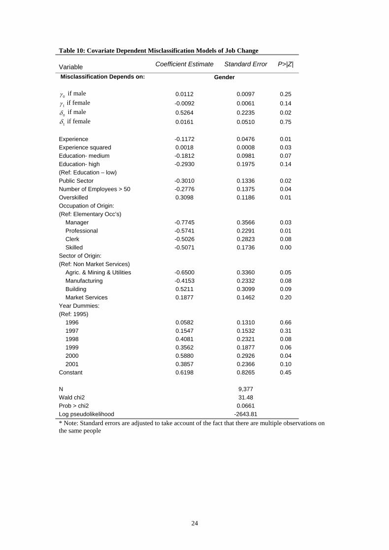
Table 10: Covariate Dependent Misclassification Models of Job Change

Variable Coefficient Estimate Standard Error P>|Z|

Misclassification Depends on: Gender

0γ if male 0.0112 0.0097 0.25

1γ if female -0.0092 0.0061 0.14

0δ if male 0.5264 0.2235 0.02

1δ if female 0.0161 0.0510 0.75 Experience -0.1172 0.0476 0.01 Experience squared 0.0018 0.0008 0.03 Education- medium -0.1812 0.0981 0.07

ducation- high -0.2930 0.1975 0.14 ef: Education – low)

ublic Sector -0.3010 0.1336 0.02 umber of Employees > 50 -0.2776 0.1375 0.04 verskilled 0.3098 0.1186 0.01 ccupation of Origin: ef: Elementary Occ’s)

Manager -0.7745 0.3566 0.03 Professional -0.5741 0.2291 0.01 Clerk -0.5026 0.2823 0.08 Skilled -0.5071 0.1736 0.00 ector of Origin: ef: Non Market Services)

Agric. & Mining & Utilities -0.6500 0.3360 0.05 Manufacturing -0.4153 0.2332 0.08 Building 0.5211 0.3099 0.09 Market Services 0.1877 0.1462 0.20 ear Dummies: ef: 1995)

1996 0.0582 0.1310 0.66 1997 0.1547 0.1532 0.31 1998 0.4081 0.2321 0.08 1999 0.3562 0.1877 0.06 2000 0.5880 0.2926 0.04 2001 0.3857 0.2366 0.10 onstant 0.6198 0.8265 0.45

9,377 ald chi2 31.48

rob > chi2 0.0661 og pseudolikelihood -2643.81

E(RPNOO(R S(R Y(R C NWPL* Note: Standard errors are adjusted to take account of the fact that there are multiple observations on

e same people th

24

7. Co ns substantial measurement error in responses to a question

re in the LIS y data on b mobility. Given the

erro s are class as bs w rocedure proposed by

is use ults cate that by ignoring misclassificat will be underestimated by

r cent. ead dim ed covariate effects. Futu ill extend this analysis to other countries in the

dataset.

nclusioThis paper finds that there isabout tenu ; the extent of which is similar to what has been found in otherstudies. Surve tenure are very often used to deduce jo

r evident in the data it is likely that caseextent of response mis ifiedhaving changed joHausman et al.

hen they truly haven’t and vice versa. A pd to control for misclassification. The resion the true number of job changes

indi

around 50 pe In addition, ignoring misclassification lre research w

s to inish

ECHP

25

26

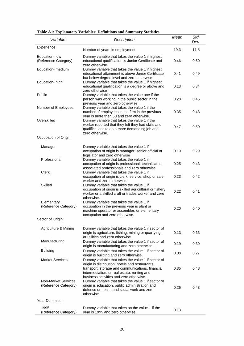
: Explanatory Va

Variable Mean Std. De

Table A1 riables: Definitions and Summary Statistics

Description v. Experience

19.3 11.5 Number of years in employment

Education- low ce Category)

ue 1 if highest 0.

n- medium unior Certificate 0.

n- high ee or above and

zero otherwise 0.13 0.34

ublic Dummy variable that takes the value one if the person was working in the public sector in the previous year and zero otherwise

0.28 0.45

umber of Employees Dummy variable that takes the value 1 if the number of employees in the firm in the previous year is more then 50 and zero otherwise.

0.35 0.48

verskilled Dummy variable that takes the value 1 if the worker reported that they felt they had skills and qualifications to do a more demanding job and zero otherwise.

0.47 0.50

ccupation of Origin:

Manager Dummy variable that takes the value 1 if occupation of origin is manager, senior official or legislator and zero otherwise

0.10 0.29

Professional Dummy variable that takes the value 1 if occupation of origin is professional, technician or associated professionals and zero otherwise

0.25 0.43

Clerk Dummy variable that takes the value 1 if occupation of origin is clerk, service, shop or sale worker and zero otherwise.

0.23 0.42

Skilled Dummy variable that takes the value 1 if occupation of origin is skilled agricultural or fishery worker or a skilled craft or trades worker and zero otherwise.

0.22 0.41

Elementary (Reference Category)

Dummy variable that takes the value 1 if occupation in the previous year is plant or machine operator or assembler, or elementary occupation and zero otherwise.

0.20 0.40

ector of Origin:

Agriculture & Mining Dummy variable that takes the value 1 if sector of origin is agriculture, fishing, mining or quarrying , or utilities and zero otherwise.

0.13 0.33

Manufacturing Dummy variable that takes the value 1 if sector of origin is manufacturing and zero otherwise. 0.19 0.39

Building Dummy variable that takes the value 1 if sector of origin is building and zero otherwise. 0.08 0.27

Market Services Dummy variable that takes the value 1 if sector of origin is distribution, hotels and restaurants, transport, storage and communications, financial intermediation, or real estate, renting and business activities and zero otherwise.

0.35 0.48

Non-Market Services (Reference Category)

Dummy variable that takes the value 1 if sector or origin is education, public administration and defence or health and social work and zero otherwise.

0.25 0.43

ear Dummies:

1995 (Reference Category)

Dummy variable that takes on the value 1 if the year is 1995 and zero otherwise. 0.13

(ReferenDummy variable that takes the valeducational qualification is Junior Certificate andzero otherwise

0.46 50

Educatio Dummy variable that takes the value 1 if highest educational attainment is above Jbut below degree level and zero otherwise Dummy variable that takes the value 1 if highest educational qualification is a degr

0.41 49

Educatio

P

N

O

O

S

Y

27

Dummy variable that takes on the value 1 if the 1996 year is 1996 and zero otherwise. 0.13

1997 Dummy variable that takes on the value 1 if the year is 1997 and zero otherwise. 0.14

1998 Dummy variable that takes on the value 1 if the year is 1998 and zero otherwise. 0.14

year is 2000 and zero otherwise. 0.15

Dummy variable that takes on the value 1 if the

1999 Dummy variable that takes on the value 1 if the year is 1999 and zero otherwise. 0.15

2000 Dummy variable that takes on the value 1 if the

2001 year is 2001 and zero otherwise. 0.16

28

8BReferences Artís, M., Ayuso, M. and M. Guillén (2002), “Detection of Automobile Insurance Fraud with Discrete Choice Models and Misclassified Claims”, The Journal of Risk and Insurance, Vol. 69, No. 3, pp. 325-340. Baker, M. and G. Solon (1999),“Earnings Dynamics and Inequality among Canadian Men, 1976-1992: Evidence from Longitudinal Income Tax Records”, NBER Working Paper No. 7370. Bound, J., Brown, C. and N. Mathiowetz (2001), “Measurement Error in Survey Data”, in J. Heckman and E. Leamer, eds, Handbook of Econometrics, Vol. 5. Brachet, T. (2005), “Maternal Smoking, Misclassification Error and Infant Health”, Working Paper. Available at: HUhttp://works.bepress.com/tbrachet/1UH. Brown, J. and A. Light (1992), “Interpreting Panel Data on Job Tenure”, Journal of Labor Economics, Vol. 10, No. 3 (Jul., 1992), pp. 219-257. Farber, S. (1999), “Mobility and Stability: The Dynamics of Job Change in Labor Markets”, in O. Ashenfelter and D. Card, eds, Handbook of Labor Economics, Vol.3. Hausman, J. (2001), “Mismeasured Variables in Econometric Analysis: Problems from the Right and Problems from the Left”, The Journal of Economic Perspectives, Vol. 15, No. 4 (Autumn 2001), pp. 57-67. Hausman, J., Abrevaya, J. and F.M. Scott-Morton (1998), “Misclassification of the dependent variable in a discrete-response setting”, Journal of Econometrics, Vol. 87, pp. 239-269. Jensen, P., Palangkaraya, A. and E. Webster (2008), “Misclassification in Patent Offices”, Intellectual Property Research Institute of Australia, Melbourne Institute of Applied Economic and Social Research, University of Melbourne, Working Paper No. 02/08, May 2008. Kenkel, D., Lillard, D. and A. Mathios (2004), “Accounting for misclassification error in retrospective smoking data”, Health Economics, Vol. 13, pp. 1031-1044. Ureta, M. (1992), “The Importance of Lifetime Jobs in the U.S. Economy, Revisited”, American Economic Review, Vol. 82, No. 1, pp. 322-335. Weiss, D., Dawis, R., England, G. and L. Lofquist (1961), “Validity of Work Histories Obtained by Interview”, Industrial Relations Center, University of Minnesota.