


Languages
Pages
Legal


Maxwell’s Equations K. Craig 1
Maxwell’s Equations
• When James Clerk Maxwell worked out his theory of
electromagnetism in 1865, he ended up with 20 equations
that describe the behavior of electric and magnetic fields.
• Oliver Heaviside in Great Britain and Heinrich Hertz in
Germany combined and simplified these equations into four
equations in the two decades after Maxwell’s death in 1879.
• Today we call these four equations – Gauss’s Law for
Electric Fields, Gauss’s Law for Magnetic Fields, Faraday’s
Law, and the Ampere-Maxwell Law – Maxwell’s Equations.
• They are on everyone’s list of the most important equations
of all time, and perhaps, they are the least understood!

Maxwell’s Equations K. Craig 2
Gauss’s Law for Electric Fields
enc
S0
qˆE nda
Electric charge produces an electric field, and the flux of that field passing through any closed surface is proportional to the total charge contained within that surface. Induced electric fields are not included here.
Integral Formvalid over a surface
Electric Flux
Total charge:free & bound
ε0 = 8.85E-12 C/(V-m)
real or imaginary surface,any size or shape
net charge

Maxwell’s Equations K. Craig 3
• An electric field is a vector and is the electrical force per
unit charge exerted on a small positive-charged object q0.
• E has units of N/C, which is the same as V/m.
• Rules of Thumb
– Electric field lines must originate on positive charge and
terminate on negative charge.
– The net electric field at any point is the vector sum of all
electric fields at that point.
– Electric field lines can never cross.
– Electric field lines are always perpendicular to the
surface of a conductor in equilibrium.
• The permittivity ε of a material determines its response to
an applied electric field.
e
0
FE
q
r
0
relativepermittivity

Maxwell’s Equations K. Craig 4
Examples of Electric Fields
Strength is shown by either the arrow length or the spacing of the lines.

Maxwell’s Equations K. Craig 5
Electric Field Equations for Simple Objects

Maxwell’s Equations K. Craig 6
• Electric Flux through a closed surface
– Electric flux is a scalar quantity and has units of electric
field times area (V-m).
– How should you think of electric flux? Use field lines, which
are continuous in space, to represent the electric field (see
previous slide of electric field examples). The strength of
the electric field at any point is indicated by the spacing of
the field lines at that location, i.e., the electric field strength
is proportional to the density of field lines (the number of
field lines per square meter) in a plane perpendicular to the
field at the point under consideration. Remember that field
lines are actually continuous in space.
– Integrating that density over the entire surface gives the net
number of field lines penetrating the surface, which is the
Electric Flux ФE, with direction of penetration taken into
account.
ES
ˆE nda
Maxwell’s Equations K. Craig 7
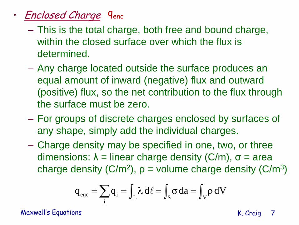
• Enclosed Charge
– This is the total charge, both free and bound charge,
within the closed surface over which the flux is
determined.
– Any charge located outside the surface produces an
equal amount of inward (negative) flux and outward
(positive) flux, so the net contribution to the flux through
the surface must be zero.
– For groups of discrete charges enclosed by surfaces of
any shape, simply add the individual charges.
– Charge density may be specified in one, two, or three
dimensions: λ = linear charge density (C/m), σ = area
charge density (C/m2), ρ = volume charge density (C/m3)
enc iL S V
i
q q d da dV
qenc
Maxwell’s Equations K. Craig 8
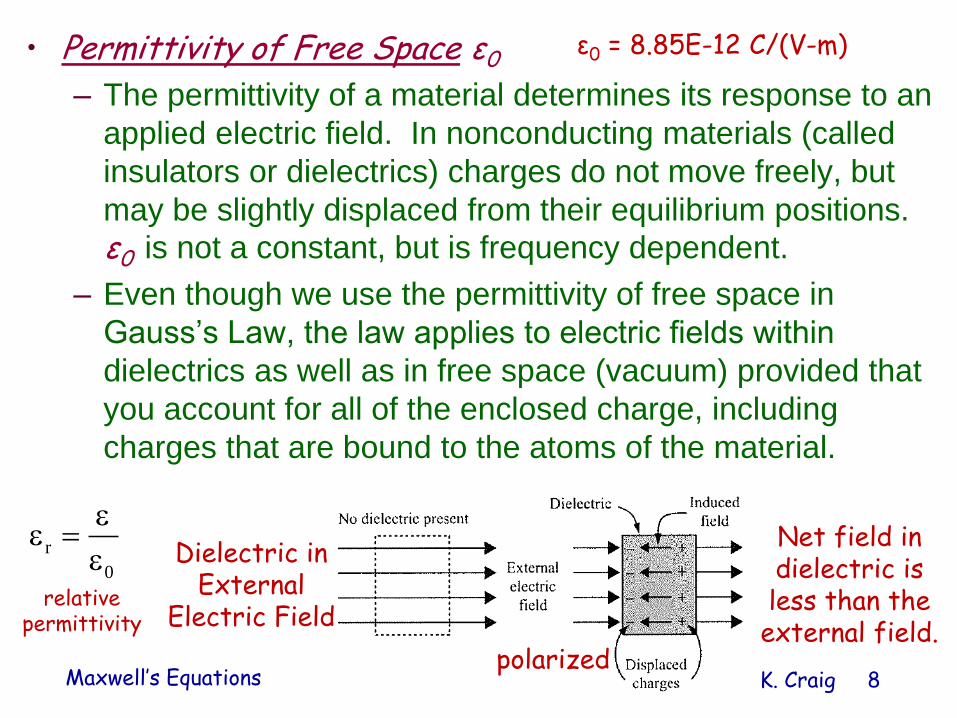
• Permittivity of Free Space ε0
– The permittivity of a material determines its response to an
applied electric field. In nonconducting materials (called
insulators or dielectrics) charges do not move freely, but
may be slightly displaced from their equilibrium positions.
ε0 is not a constant, but is frequency dependent.
– Even though we use the permittivity of free space in
Gauss’s Law, the law applies to electric fields within
dielectrics as well as in free space (vacuum) provided that
you account for all of the enclosed charge, including
charges that are bound to the atoms of the material.
ε0 = 8.85E-12 C/(V-m)
Dielectric in External
Electric Field
Net field in dielectric is less than the
external field.polarized
r
0
relative
permittivity

Maxwell’s Equations K. Craig 9
Differential Formvalid at individual points
in space
0
E
The electric field produced by electric charge diverges from positive charge and converges upon negative charge.
Divergence of E Field:tendency of E field to
“flow” away from positivecharge
ˆ ˆ ˆi j kx y z
SV 0
1ˆE lim E nda
V
yx zEE E
Ex y z
scalar
Only places where the divergence is not zero are those locations where charge is present.

Maxwell’s Equations K. Craig 10
• Both flux and divergence deal with the “flow” of a vector
field, but with an important difference; flux is defined over
an area, while divergence applies to individual points.
• Points of positive divergence are sources (positive charge),
while points of negative divergence are sinks (negative
charge).
• The mathematical definition of divergence may be
understood by considering the flux through an infinitesimal
surface surrounding the point of interest. If you were to
form the ratio of the flux of a vector field through a surface
to the volume enclosed by that surface as the volume
shrinks toward zero, you would have the divergence of the
vector field:
SV 0
1ˆE lim E nda
V

Maxwell’s Equations K. Craig 11
Vector Fields with Various Values of Divergence
Positive Divergence: Points 1, 2, 3, and 5Negative Divergence: Point 4Zero Divergence: Points 6 and 7, as the flow lines are spreading out but also getting shorter at greater distance from the center. The spreading out compensates for the slowing down of the flow.Note: The key factor in determining the divergence at any point is whether the flux out of an infinitesimally small volume around the point is greater than, equal to, or less than the flux into the volume.

Maxwell’s Equations K. Craig 12
Gauss’s Law for Magnetic Fields
SˆB nda 0
The total magnetic flux passing through any closed surface is zero. The inward magnetic flux must be exactly balanced by the outward magnetic flux.
Integral Formvalid over a surface
Magnetic Flux
real or imaginary surface,any size or shape
Maxwell’s Equations K. Craig 13
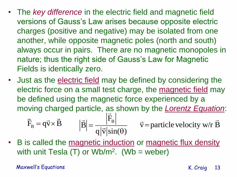
• The key difference in the electric field and magnetic field
versions of Gauss’s Law arises because opposite electric
charges (positive and negative) may be isolated from one
another, while opposite magnetic poles (north and south)
always occur in pairs. There are no magnetic monopoles in
nature; thus the right side of Gauss’s Law for Magnetic
Fields is identically zero.
• Just as the electric field may be defined by considering the
electric force on a small test charge, the magnetic field may
be defined using the magnetic force experienced by a
moving charged particle, as shown by the Lorentz Equation:
• B is called the magnetic induction or magnetic flux density
with unit Tesla (T) or Wb/m2. (Wb = weber)
BF qv B BFB
q v sin( )
v particlevelocity w/r B

Maxwell’s Equations K. Craig 14
• Distinctions between Magnetic and Electric Fields
– Like the electric field, the magnetic field is directly proportional
to the magnetic force. But unlike the electric field, which is
parallel or antiparallel to the electric force, the direction of the
magnetic field is perpendicular to the magnetic force.
– Like the electric field, the magnetic field may be defined
through the force experienced by a small test charge, but
unlike the electric field, the speed and direction of the test
charge must be taken into consideration when relating
magnetic forces and fields.
– Because the magnetic force is perpendicular to the velocity at
every instant, the component of the force in the direction of the
displacement is zero, and the work done by the magnetic field
is therefore always zero.
– Whereas electrostatic fields are produced by electric charges,
magnetostatic fields are produced by electric currents.

Maxwell’s Equations K. Craig 15
Examples of Magnetic FieldsMagnetic fields may be represented using field lines whose density in a plane perpendicular to the line direction is proportional to the strength of the field. Don’t forget that magnetic fields, like electric fields, are continuous in space.

Maxwell’s Equations K. Craig 16
• Rules of Thumb
– Magnetic field lines do not originate and terminate on
charges; they form closed loops.
– The magnetic field lines that appear to originate on the
north pole and terminate on the south pole of a magnet
are actually continuous loops (within the magnet, the
field lines run between the poles).
– The net magnetic field at any point is the vector sum of
all magnetic fields present at that point.
– Magnetic field lines can never cross, since that would
indicate that the field points in two different directions at
the same location – if the fields from two or more
sources overlap at the same location, they add (as
vectors) to produce a single, total field at that point.

Maxwell’s Equations K. Craig 17
• All static magnetic fields are produced by moving electric
charge. The contribution to the magnetic field at a specified
point P from a small element of electric current is given by
the Biot-Savart Law:
• µ0 is the permeability of free space and I is the current.
• Magnetic Flux, like Electric Flux, is a scalar quantity. The
unit is webers (Wb = T-m2). Outward and inward magnetic
flux must be equal and opposite through any closed surface;
magnetic field lines always form complete loops.
0
2
ˆId rdB
4 r

Maxwell’s Equations K. Craig 18
Magnetic Field Equations for Simple Objects

Maxwell’s Equations K. Craig 19
Differential Formvalid at individual points
B 0
Divergence of B Field
The divergence of the magnetic field at any point is zero. Since it is not possible to isolate magnetic poles, you can’t have a north pole without a south pole, and the “magnetic charge density” must be zero everywhere.
Vector fields with zero divergence are called “solenoidal” fields, and all magnetic fields are solenoidal.

Maxwell’s Equations K. Craig 20
Faraday’s Law
Integral Form
C S
dˆE d B nda
dt
Changing magnetic flux through a surface induces an emf in any boundary path of that surface, and a changing magnetic field induces a circulating electric field.
The negative sign tells us that the induced emf opposes the change in flux, i.e., it tends to maintain the existing flux. This is called Lenz’s Law.
E in this expression is the induced electric field at each segment of the path C measured in the reference frame in which that segment is stationary.
circulation of Earound path C

Maxwell’s Equations K. Craig 21
• Induced Electric Field
– Charge-based electric fields have fields that originate on
positive charge and terminate on negative charge, and
thus have non-zero divergence at those points.
– Induced electric fields produced by changing magnetic
fields have field lines that loop back on themselves, with
no points of origination or termination, and thus have
zero divergence.
Both types of electric field accelerate electric charges and are represented by field lines, but are different in structure.

Maxwell’s Equations K. Craig 22
• Electric Field Circulation
– Since the field lines of induced electric fields form closed loops,
these fields are capable of driving charged particles around
continuous circuits, i.e., generate an electric current. The
circulation of the electric field around a circuit is known as
electromotive force (emf). It is not actually a force, but rather a
force per unit charge integrated over a distance.
– So the circulation of the induced electric field around a path is
the work done by the electric field in moving a unit charge
around that path; it is the energy given to each coulomb of
charge as it moves around the circuit.
CE d Electric Field Circulation = electromotive force (emf)
C
C C
F dF WE d d
q q q

Maxwell’s Equations K. Craig 23
• Rate of Change of Flux
– This expression represents the rate of change of
magnetic flux through any surface. How can the
magnetic flux through a surface change with time?
• The magnitude of vector B might change.
• The angle between vector B and the surface normal
might change.
• The area of the surface S might change.
BS
d dˆB nda = Rate of Change of Flux
dt dt
Note that the magnitude of the induced emf depends only on how
fast the flux changes.
Maxwell’s Equations K. Craig 24
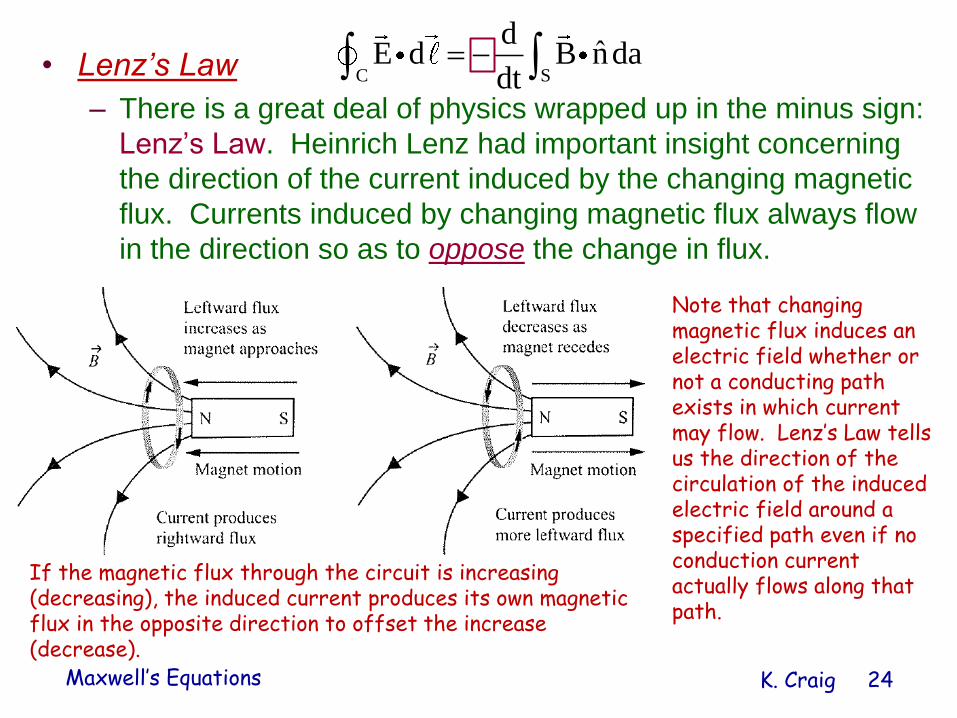
• Lenz’s Law
– There is a great deal of physics wrapped up in the minus sign:
Lenz’s Law. Heinrich Lenz had important insight concerning
the direction of the current induced by the changing magnetic
flux. Currents induced by changing magnetic flux always flow
in the direction so as to oppose the change in flux.
C S
dˆE d B nda
dt
Note that changing magnetic flux induces an electric field whether or not a conducting path exists in which current may flow. Lenz’s Law tells us the direction of the circulation of the induced electric field around a specified path even if no conduction current actually flows along that path.
If the magnetic flux through the circuit is increasing (decreasing), the induced current produces its own magnetic flux in the opposite direction to offset the increase (decrease).

Maxwell’s Equations K. Craig 25
BE
t
A circulating electric field is produced by a magnetic field that changes with time.Curl of
electric field
CS 0
1E lim E d
S
Curl of the electric field is a measure of the E field’s tendency to circulate about a point. The direction of the curl is the normal direction of the surface for which the circulation is a maximum.
Differential Formvalid at individual points

Maxwell’s Equations K. Craig 26
• Curl of a Vector Field – measure of the field’s tendency to
circulate about a point.
– To physically understand the concept of curl, imagine
holding a tiny paddlewheel at each point in a flow. If the flow
would cause the paddlewheel to rotate, the center of the
wheel marks a point of nonzero curl. The direction of the
curl is along the axis of the paddlewheel, with the positive-
curl direction determined by the right-hand rule.
– Vector fields with zero curl at all points are called irrotational.
x y z
y yz x z x
ˆ ˆ ˆi j kx y z
ˆ ˆ ˆ ˆ ˆ ˆE i j k iE jE kEx y z
E EE E E Eˆ ˆ ˆi j ky z z x x y
Each component indicates the tendency of the field to rotate in one of the coordinate planes. The overall direction represents the axis about which the rotation is greatest, with the sense of rotation given by the right-hand rule.

Maxwell’s Equations K. Craig 27
Vector Fields with Various Values of Curl
High-Curl Locations: Points 1, 2, 3, 4, and 5Zero-Curl Locations: Points 6 and 7

Maxwell’s Equations K. Craig 28
• Curl of the Electric Field
– Charge-based electric fields diverge away from points
of positive charge and converge toward points of
negative charge. Such fields cannot circulate back on
themselves. All electrostatic fields have no curl.
– Electric fields induced by changing magnetic fields are
very different. Whenever a changing magnetic field
exists, a circulating electric field is induced. Unlike
charge-based electric fields, induced fields have no
origination or termination points – they are continuous
and circulate back on themselves. Integrating
around any boundary path for the surface through
which is changing produces a nonzero result, which
means that induced electric fields have curl. The
faster changes, the larger the magnitude of the curl
of the induced electric field.
E d
B
B

Maxwell’s Equations K. Craig 29
Ampere-Maxwell Law
Integral Form
0 enc 0C S
dˆB d I E nda
dt
An electric current or a changing electric flux through a surface produces a circulating magnetic field around any path that bounds that surface.
Circulation of magnetic field around closed
path C
A magnetic field is produced along a path (real or imaginary) if any current is enclosed by the path or if the electric flux through any surface bounded by the path changes over time.

Maxwell’s Equations K. Craig 30
• Some Background
– Ampere’s Law relating a steady electric current to
a circulating magnetic field was well known when
Maxwell began his work in the 1850s.
– However, Ampere’s Law was known to apply only
to static situations involving steady currents.
Maxwell added another source term – a changing
electric flux – that extended the applicability of
Ampere’s Law to time-dependent conditions.
– It was the presence of this term in the equation,
now called the Ampere-Maxwell Law, that allowed
Maxwell to discern the electromagnetic nature of
light and to develop a comprehensive theory of
electromagnetism.

Maxwell’s Equations K. Craig 31
• Magnetic Field Circulation
– Shown is the magnetic field around a current-carrying
wire.
– The magnetic field strength decreases precisely as 1/r,
where r is the distance from the wire.
– As you circle around the wire, the direction of the
magnetic field is along your path, perpendicular to an
imaginary line from the wire to your location.
CB d

Maxwell’s Equations K. Craig 32
• Permeability of Free Space (vacuum) µ0 = 4π x 10-7 Vs/Am
– Just as the electric permittivity characterizes the
response of a dielectric to an applied electric field, the
magnetic permeability determines a material’s response
to an applied magnetic field.
– As in the case of electric permittivity in Gauss’s Law for
electric fields, the presence of this quantity does not
mean that the Ampere-Maxwell Law applies only to
sources and fields in a vacuum. This form of the
Ampere-Maxwell Law is general, so long as you consider
all currents, bound as well as free.
– Unlike the effect of dielectrics on electric fields, the effect
of magnetic substances on magnetic fields is that the
magnetic field is actually stronger than the applied field
within many magnetic materials.
Maxwell’s Equations K. Craig 33
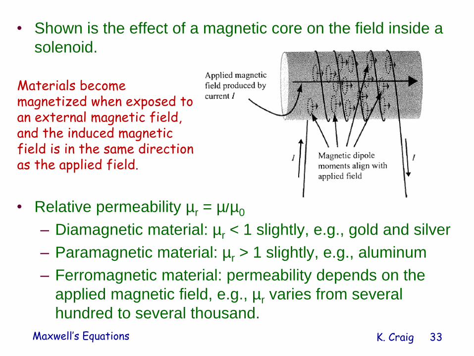
• Shown is the effect of a magnetic core on the field inside a
solenoid.
• Relative permeability µr = µ/µ0
– Diamagnetic material: µr < 1 slightly, e.g., gold and silver
– Paramagnetic material: µr > 1 slightly, e.g., aluminum
– Ferromagnetic material: permeability depends on the
applied magnetic field, e.g., µr varies from several
hundred to several thousand.
Materials become magnetized when exposed to an external magnetic field, and the induced magnetic field is in the same direction as the applied field.
Maxwell’s Equations K. Craig 34
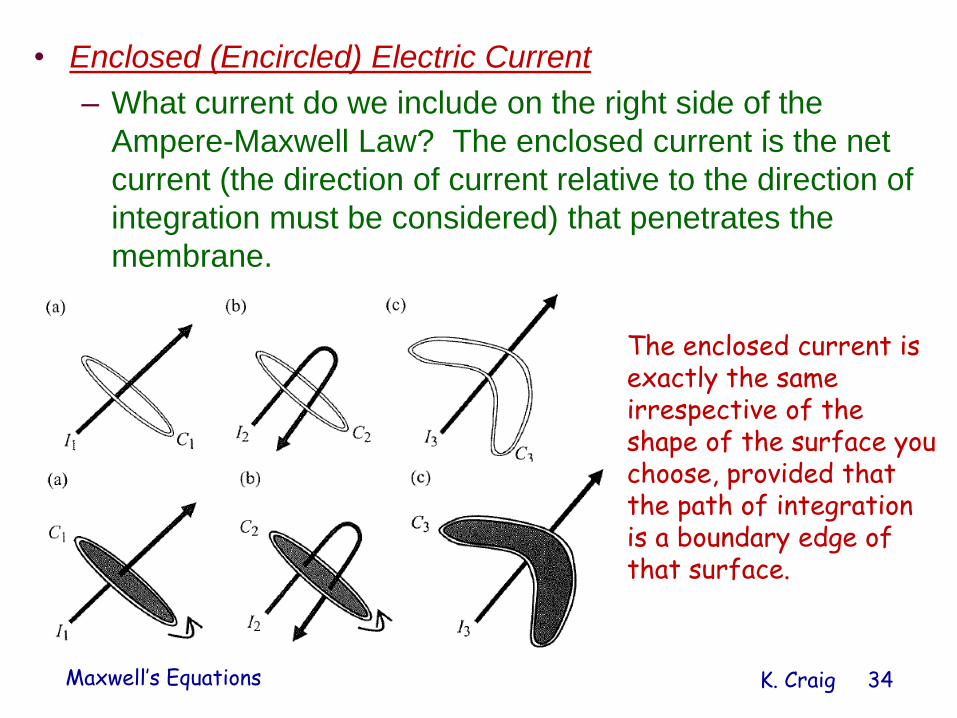
• Enclosed (Encircled) Electric Current
– What current do we include on the right side of the
Ampere-Maxwell Law? The enclosed current is the net
current (the direction of current relative to the direction of
integration must be considered) that penetrates the
membrane.
The enclosed current is exactly the same irrespective of the shape of the surface you choose, provided that the path of integration is a boundary edge of that surface.

Maxwell’s Equations K. Craig 35
• Rate of Change of Flux
– This term is the electric flux analog of the changing
magnetic flux term in Faraday’s Law.
– To demonstrate the need for the changing-flux term in
the Ampere-Maxwell Law, we can study the
inconsistency in Ampere’s law when applied to a
charging capacitor.
S
dˆE nda
dt
0 encC
B d I
E
S S S0 0 0
Q / A QˆE nda da da
0 dS
d dQˆE nda I displacement current
dt dt
No conduction current flows between capacitor plates.
σ is charge density on plates = Q/A.
Even though no charge actually flows.

Maxwell’s Equations K. Craig 36
0 0
EB J
t
Differential Form
A circulating magnetic field is produced by an electric current and by an electric field that changes with time.
curl of the magnetic field electric current density &
time rate of change of electric field
The curl of the magnetic field is nonzero exactly at the location through which an electric current is flowing, or at which an electric field is changing.
All magnetic fields circulate back on themselves and form continuous loops.

Maxwell’s Equations K. Craig 37
• Curl of the Magnetic Field
– All magnetic fields, whether produced by electric
currents or by changing electric fields, circulate back
upon themselves and form continuous loops.
– In addition, all fields that circulate back on themselves
must include at least one location about which the path
integral of the field is nonzero. For the magnetic field,
locations of nonzero curl are locations at which current is
flowing or an electric field is changing.
– Just because magnetic fields circulate, do not conclude
that the curl is nonzero everywhere in the field. A
common misconception is that the curl of a vector field is
nonzero wherever the field appears to curve.
– How can a curving field have zero curl?
B

Maxwell’s Equations K. Craig 38
– The answer lies in the amplitude as well as the
direction of the magnetic field.
Offsetting components of the curl of the magnetic field using the fluid-flow and small paddlewheel analogy
The key concept is that the magnetic field may be curved at many different locations, but only at points at which
the current is flowing (or the electric flux is changing) is the curl of the B vector nonzero.

Maxwell’s Equations K. Craig 39
• Electric Conduction Current Density
– This is defined as the vector current flowing
through a unit cross-sectional area perpendicular
to the direction of the current.
– The units of current density are amperes per
square meter (A/m2).
– The electric current density includes all currents,
including the bound current density in magnetic
materials.

Maxwell’s Equations K. Craig 40
• Displacement Current Density
– This term involves the rate of change of the
electric field with time. This has units of amperes
per square meter (A/m2), identical to those of
electric conduction current density, J.
– Does the displacement current density represent
an actual current? Not in the conventional sense!
But the displacement current density is a vector
quantity that has the same relationship to the
magnetic field as does the conduction current
density, J.
– The key concept is that a changing electric field
produces a changing magnetic field even when no
charges are present and no physical current flows.
0
E
t

Maxwell’s Equations K. Craig 41
Summary

Maxwell’s Equations K. Craig 42
One More Thing…
• Gradient
– The third differential operator (divergence and curl are the
other two operators) is the gradient.
– The gradient applies to scalar fields, i.e., a field that is
specified by only its magnitude at various locations.
– What does the gradient tell you about a scalar field? Two
important things: the magnitude of the gradient indicates how
quickly the field is changing over space, and the direction of
the gradient indicates the direction in that the field is
changing most quickly with distance.
– The result of the gradient operation is a vector, with both
magnitude and direction.
ˆ ˆ ˆi j kx y z
Note this identity: 0

Maxwell’s Equations K. Craig 43
Electrostatics & Magnetostatics
• The static form of Maxwell’s Equations are derived from the
complete forms by imposing the conditions that there are no
time varying E and B fields. Mathematically, these
conditions are represented by the requirements that:
• Maxwell’s Equations then are: E B0 0
t t
enc
S0
qˆE nda
SˆB nda 0
CE d 0
0 encC
B d I
0
E
B 0
E 0
0B J
Each equation is a function of either E or B; no equation contains both E and B. Electric and magnetic fields are uncoupled; electricity and magnetism are independent subjects.

Maxwell’s Equations K. Craig 44
Quasistatics
• Quasistatics reside between electrostatics and
magnetostatics (no time changes) and electrodynamics
(fully dynamic coupled behavior).
• The primary significance of quasistatics is that it establishes
the foundations of modern circuit theory.
• When electric field effects dominate magnetic field effects,
the laws of electroquasistatics result.
• When magnetic field effects dominate electric field effects,
the laws of magnetoquasistatics result.
• What are the quantitative criteria under which these laws
are applicable?
Maxwell’s Equations K. Craig 45
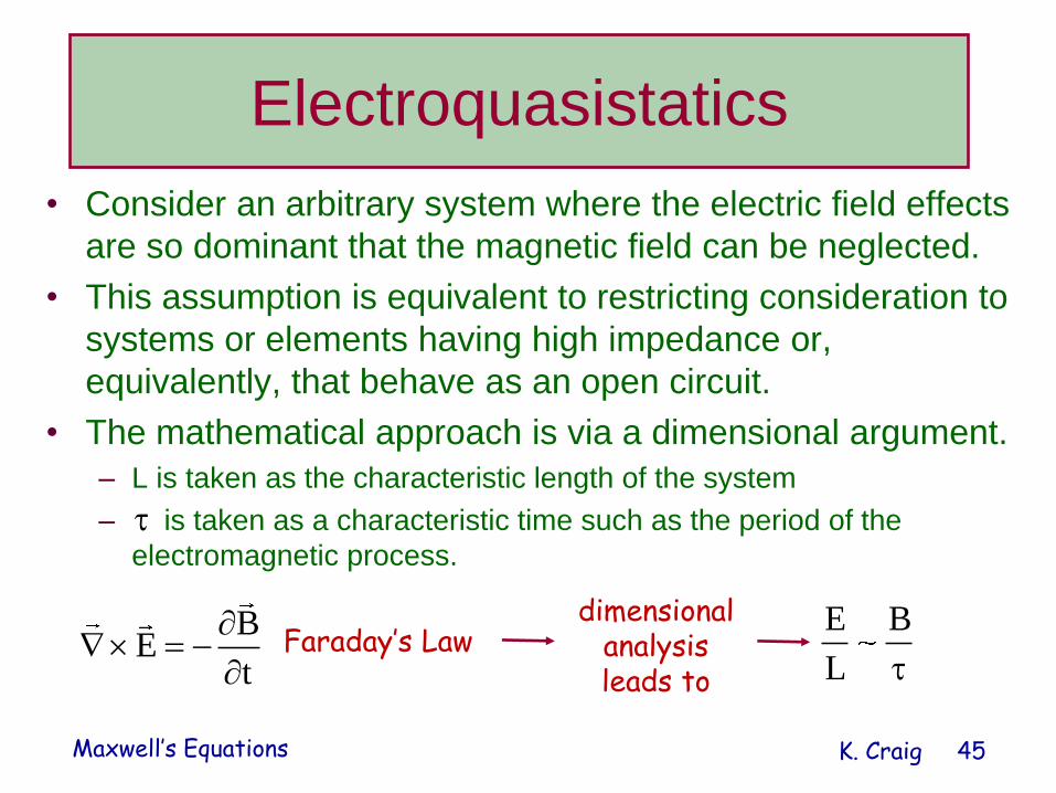
Electroquasistatics
• Consider an arbitrary system where the electric field effects
are so dominant that the magnetic field can be neglected.
• This assumption is equivalent to restricting consideration to
systems or elements having high impedance or,
equivalently, that behave as an open circuit.
• The mathematical approach is via a dimensional argument.
– L is taken as the characteristic length of the system
– is taken as a characteristic time such as the period of the
electromagnetic process.
BE
t
Faraday’s Law
E B
L
dimensional analysis leads to

Maxwell’s Equations K. Craig 46
• For magnetic effects to be negligible compared with the
electric field effects
• Now consider
E B
L
0 0
EB J
t
Ampere-Maxwell Law
In a high-impedance system, e.g., a capacitor, the current density term will be negligibly small compared with the displacement current because no charge can be transported across the open space. It is the field-induced current, rather than the flow of charge across the gap of a capacitor that is primarily responsible for the current through a capacitor.
dimensional analysis leads to
0 0
B E
L
2
B 1 E
L c
2
0 0
1c
2
1 ELB
c
c = speed of light

Maxwell’s Equations K. Craig 47
• Substitution
• We know
2
1 ELB
c
E B
L
2 2
E EL
L c
L1
c
This is an important result; it is a quantitative criterion for the appropriate application of electroquasistatics. The characteristic time or period of the electromagnetic process must be sufficiently long to ensure that L
1c
1and
c f
L1
c
L1
Lf1
c
λ = wavelengthf = frequency
Alternative expressions to assess the electroquasistatic approximation:
Maxwell’s Equations K. Craig 48
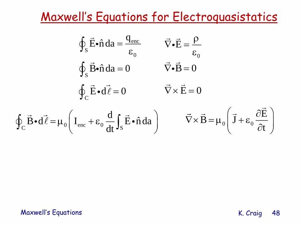
enc
S0
qˆE nda
SˆB nda 0
CE d 0
0
E
B 0
E 0
0 enc 0C S
dˆB d I E nda
dt
0 0
EB J
t
Maxwell’s Equations for Electroquasistatics

Maxwell’s Equations K. Craig 49
Magnetoquasistatics
• Consider an arbitrary system where the magnetic field
effects are so dominant that the electric field can be
neglected.
• This assumption is equivalent to restricting consideration to
systems or elements having low impedance or,
equivalently, that behave as a short circuit.
• The mathematical approach is via a dimensional argument.
– L is taken as the characteristic length of the system
– is taken as a characteristic time such as the period of the
electromagnetic process.

Maxwell’s Equations K. Craig 50
• Consider the Ampere-Maxwell Equation
– It is necessary for the B field to be much more dominant
than the E field. This implies that the entire displacement
current must be negligible. This is possible only if it is
much smaller than both the current density term and the
magnetic field term. Alternatively, it means that both the J
and B terms need to be much larger than the
displacement current term.
– In order for the J term to be large, the system under
consideration must be of low impedance or behave like a
short circuit, e.g., a system consisting of a conducting
wire loop (an inductor) where the J effects will be large
compared with the E effects.
0 0
EB J
t

Maxwell’s Equations K. Craig 51
• Apply the dimensional argument to the Ampere-Maxwell
Law, requiring that the B field term be much larger than
the E field term. This results in the inequality
• From Faraday’s Law
• Substitution leads to
0 0
B E
L
BE
t
Faraday’s Law
E B
L
dimensional analysis leads to
0 0 2
B BL
L
L1
c
2
0 0
1c
The condition that must be satisfied to ensure validity of magnetoquasistatics is the same as that for electroquasistatics.

Maxwell’s Equations K. Craig 52
enc
S0
qˆE nda
SˆB nda 0
0
E
B 0
BE
t
0 encC
B d I 0B J
C S
dˆE d B nda
dt
Maxwell’s Equations for Magnetoquasistatics

Maxwell’s Equations K. Craig 53
• In electroquasistatics, the change from the complete form of
Maxwell’s Equations is in Faraday’s law. Here the term
has been removed from the complete form of Faraday’s
Law. In magnetoquasistatics, the change is in Ampere’s
Law; the displacement current term has been removed.
• In quasistatics there is a decoupling of the electric and
magnetic fields, similar to statics; however, this decoupling
is partial but, unlike statics, it maintains a time variation of
the E and B fields.
• Electroquasistatics is dependent only on the time variations
in the E field. Magnetoquasistatics is dependent only on the
time variations in the B field.
• We now look at how energy in electroquasistatics and
magnetoquasistatics is stored via the E and B fields,
respectively.
B
t

Maxwell’s Equations K. Craig 54
Energy Storage
• Here we consider energy storage in electroquasistatics
and magnetoquasistatics. The results of this analysis
illustrate further the consequences of the decoupling of
the E and B fields in quasistatics.
• We will show that the electromagnetic energy is stored in
the electric field for systems characterized by the
electroquasistatics approximation while the
electromagnetic energy is stored in the magnetic field for
systems characterized by the magnetoquasistatic
approximation.

Maxwell’s Equations K. Craig 55
• Shown is an energy balance in volume V bounded by
closed surface S.
dS V VP dS wdV p dV
t
Rate of energy flow into the system
through surface S (Ein)
Energy accumulation rate in the system
volume V (Ea)
Energy dissipation rate in the system
volume V (Ed)
P is the rate of energy flow per unit area through the surface S into the volume V. w is the energy density within V and pd is the rate of dissipation of the energy density within V.
Ein = Ea + Ed
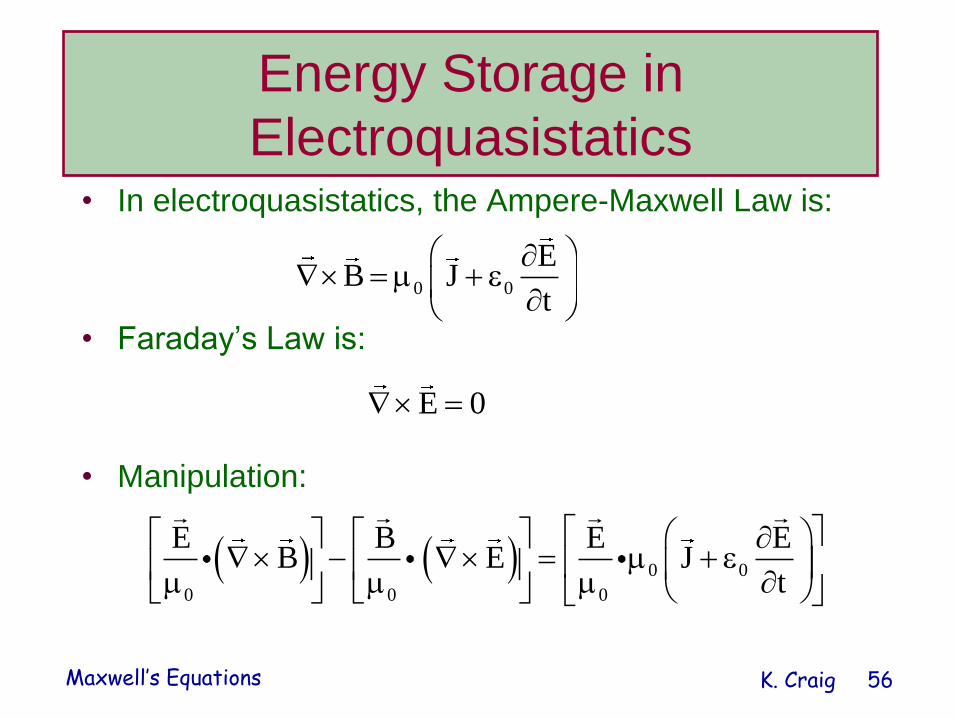
Maxwell’s Equations K. Craig 56
Energy Storage in
Electroquasistatics• In electroquasistatics, the Ampere-Maxwell Law is:
• Faraday’s Law is:
• Manipulation:
0 0
EB J
t
E 0
0 0
0 0 0
E B E EB E J
t

Maxwell’s Equations K. Craig 57
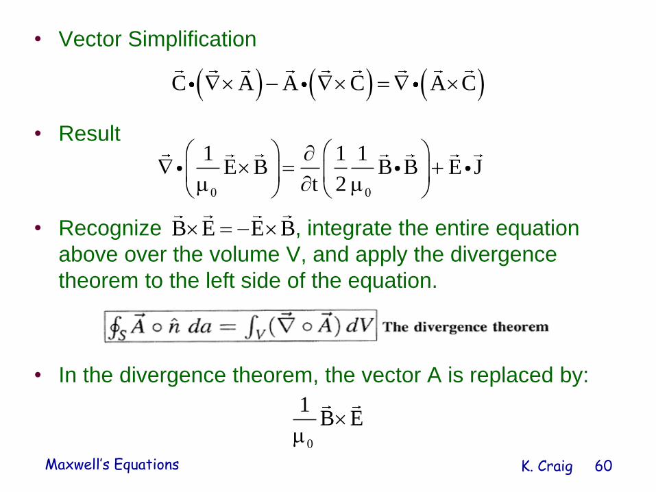
• Vector Simplification
• Result
• Recognize , integrate the entire
equation above over the volume V, and apply the
divergence theorem to the left side of the equation.
• In the divergence theorem, the vector A is replaced
by:
C A A C A C
0
0
1 1B E E E E J
t 2
B E E B
0
1B E

Maxwell’s Equations K. Craig 58
• Result:
• We see that:
• Energy accumulation is accomplished via the E field. In an
element or system characterized by the electroquasistatic
approximation (e.g., ideal capacitor), the energy is stored in
the electric field.
dS V VP dS wdV p dV
t
0S V V
0
1 1E B dS E E dV E J dV
t 2
0
0
1P E B rate of energy flux
1w E E electromagnetic energy density
2

Maxwell’s Equations K. Craig 59
Energy Storage in
Magnetoquasistatics
• In magnetoquasistatics, the Ampere-Maxwell Law is:
• Faraday’s Law is:
• Manipulation:
0B J
BE
t
0 0 0
E B B BB E E J
t
Maxwell’s Equations K. Craig 60
• Vector Simplification
• Result
• Recognize , integrate the entire equation
above over the volume V, and apply the divergence
theorem to the left side of the equation.
• In the divergence theorem, the vector A is replaced by:
C A A C A C
0 0
1 1 1E B B B E J
t 2
B E E B
0
1B E

Maxwell’s Equations K. Craig 61
• Result:
• We see that:
• Energy accumulation is accomplished via the B field. In
an element or system characterized by the
magnetoquasistatic approximation (e.g., ideal inductor),
the energy is stored in the magnetic field.
dS V VP dS wdV p dV
t
S V V0 0
1 1 1E B dS B B dV E J dV
t 2
0
0
1P E B rate of energy flux
1 1w B B electromagnetic energy density
2

Maxwell’s Equations K. Craig 62
Kirchhoff’s “Laws”
• The fundamental concepts of modern circuit theory can be
derived as a consequence of quasistatics. The formulation of
the equations of motion for an electrical network via circuit
theory requires the satisfaction of three steps:
– Kirchhoff’s Current “Law”
– Kirchhoff’s Voltage “Law”
– Constitutive relations for the individual elements
• One of the major consequences of quasistatics that is utilized
in circuit theory is that the electric and magnetic fields are
highly localized in the capacitive and inductive elements,
respectively, and negligible elsewhere. Fields exist only within
the capacitive and inductive elements, not at nodes.

Maxwell’s Equations K. Craig 63
Kirchhoff’s Current “Law”
• Quasistatic Ampere-Maxwell Law applied to a node
in an electrical network is , as the E and B
fields are negligible at a node.encI 0
r
k
k 1
i 0
Maxwell’s Equations K. Craig 64
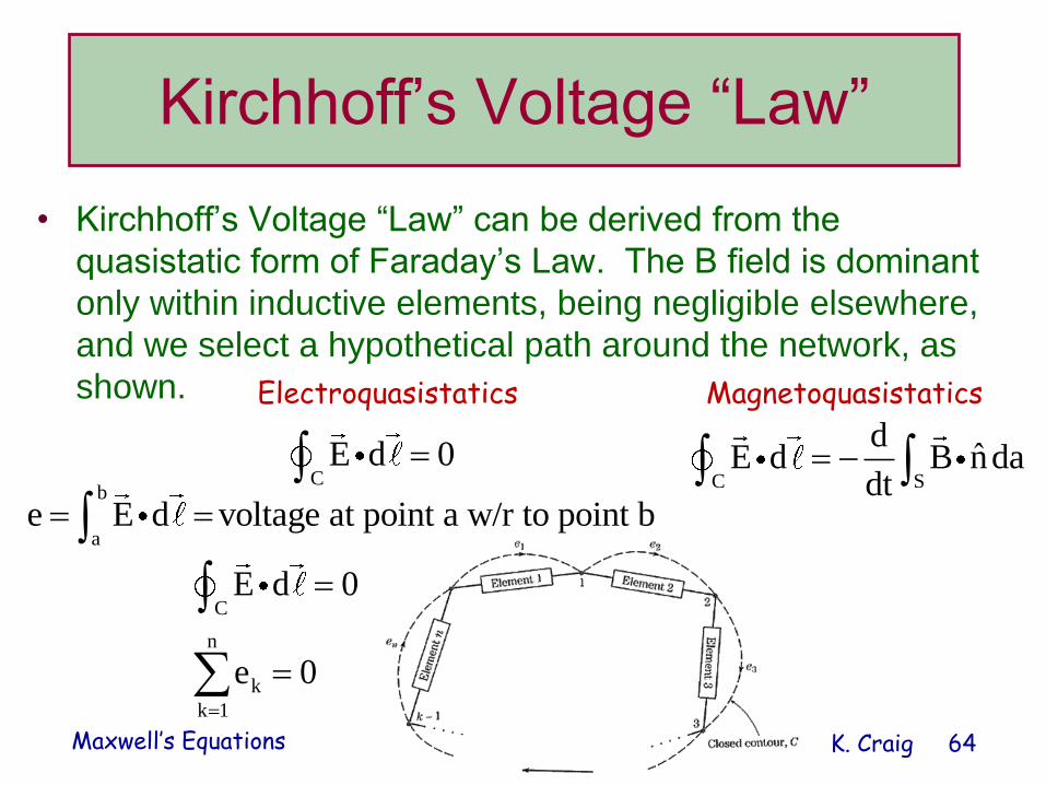
Kirchhoff’s Voltage “Law”
• Kirchhoff’s Voltage “Law” can be derived from the
quasistatic form of Faraday’s Law. The B field is dominant
only within inductive elements, being negligible elsewhere,
and we select a hypothetical path around the network, as
shown.
CE d 0
C S
dˆE d B nda
dt
Electroquasistatics Magnetoquasistatics
b
ae E d voltage at point a w/r to point b
C
n
k
k 1
E d 0
e 0
Top Related