


Languages
Pages
Legal


University of Pretoria Department of Economics Working Paper Series
LPPLS Bubble Indicators over Two Centuries of the S&P 500 Index Qunzhi Zhang Eidgenössische Technische Hochschule Zürich Didier Sornette Eidgenössische Technische Hochschule Zürich and University of Geneva Mehmet Balcilar Eastern Mediterranean University, University of Pretoria and IPAG Business School Rangan Gupta University of Pretoria Zeynel A. Ozdemir Gazi University and Economic Research Forum (ERF) Hakan Yetkiner Izmir University of Economics Working Paper: 2016-06 February 2016 __________________________________________________________ Department of Economics University of Pretoria 0002, Pretoria South Africa Tel: +27 12 420 2413
1
LPPLS Bubble Indicators over Two Centuries of the S&P 500 Index
Qunzhi Zhang
ETH Zurich, Department of Management, Technology and Economics (D-MTEC) Scheuchzerstrasse 7, CH-8092 Zurich, Switzerland
E-mail address: [email protected]
Didier Sornette* ETH Zurich, Department of Management, Technology and Economics, ,Scheuchzerstrasse 7, CH-8092 Zurich, Switzerland; Swiss Finance Institute, c/o University of Geneva, 40 blvd. Du
Pont d’Arve, CH-1211 Geneva 4, Switzerland E-mail address: [email protected]
Mehmet Balcilar
Department of Economics, Eastern Mediterranean University, Famagusta, Turkish Republic of Northern Cyprus, via Mersin 10, Turkey; Department of Economics, University of Pretoria,
Pretoria, 0002, South Africa; and IPAG Business School, Paris France E-mail address: [email protected]
Rangan Gupta
Department of Economics, University of Pretoria, Pretoria, 0002, South Africa E-mail address: [email protected]
Zeynel Abidin Ozdemir
Department of Economics, Gazi University, Besevler, 06500, Ankara, Turkey; and Economic Research Forum (ERF), Cairo
E-mail address: [email protected]
Hakan Yetkiner Department of Economics, Izmir University of Economics, Balcova, 35330, Izmir, Turkey
E-mail address: [email protected]
Abstract The aim of this paper is to present novel tests for the early causal diagnostic of positive and negative bubbles in the S&P 500 index and the detection of End-of-Bubble signals with their corresponding confidence levels. We use monthly S&P 500 data covering the period from August 1791 to August 2014. This study is the first work in the literature showing the possibility to develop reliable ex-ante diagnostics of the frequent regime shifts over two centuries of data. We show that the DS LPPLS (log-periodic power law singularity) approach successfully diagnoses positive and negative bubbles, constructs efficient End-of-Bubble signals for all of the well-documented bubbles, and obtains for the first time new statistical evidence of bubbles for some other events. We also compare the DS LPPLS method to the exponential curve fitting and the generalized sup ADF test approaches and find that DS LPPLS system is more accurate in identifying well-known bubble events, with significantly smaller numbers of false negatives and false positives.
Keywords: S&P 500, LPPL method, stock market bubble, forecast, bubble indicators JEL classification: J16, O47, C32
* Corresponding author.

2
I. Introduction
The US market capitalization of firms rose from $2.8 trillion in the end of 1988
to $18.7 trillion in the end of 2012 in current prices and hence increased 6.7
times in 15 years or 13.5% per year in average compounded growth.
Correspondingly, $1.8 trillion in the end of 1998 and $9.6 trillion in the end of
2012 of corporate equities was held by households and non-profit organizations
in the US.1 Given the level of penetration of the stock market investment in US,
a boom or a bust in the market has widespread effects on US economy, beyond
its effect on the wealth of households and the value of firms. Therefore, it is
vital to diagnose booms and busts before they hit the stock market.
The S&P 500 (S&P500) is one of the most frequently used stock market
index in gauging the US stock market performance. The S&P price index, like
many other assets, shows positive and negative bubbles in certain periods,
which seems to contradict with the Efficient Market Hypothesis. Since Sornette
et al. (1996), there is a growing research using critical points with log-periodic
corrections, borrowed from statistical physics, in identifying bubbles.2 This
methodology (later started to be called Johansen-Ledoit-Sornette (JLS) model or
Log-Periodic Power Law Singularity (LPPLS) analysis) proposes that a bubble
can emerge intrinsically out of the natural functioning of the market. A brief
survey of this literature is as follows.3 To further test the methodology, Sornette
and Johansen (1997) used the two largest historical crashes of the century, the
October 1929 and October 1987 crashes, and showed that the methodology
identifies the two crashes by analysis bubbles developing over an interval of 8
years prior to when they happened. Sornette and Johansen (1998) presented a
simple hierarchical model of traders in stock markets, e.g., currency blocks at
the highest level of the hierarchy, the countries at the next level, major banks 1 See Balance Sheet of Households and Nonprofit Organizations (B.100) in Financial Accounts of the United States. 2 See Sornette (1998) demonstrating the analogies between the quantification of risks in finance and insurance and the optimization of portfolios on one hand and statistical physics concepts and methods on the other. 3 Extended and condensed reviews of the literature can be found in Sornette (2003a) and Sornette et al. (2013), respectively.

3
and institutions within a country then, and so forth, all exhibiting herd behavior.
Sornette and Johansen (1998) showed that this hierarchical organization was
sufficient to produce log-periodic oscillations and that a systemic instability
could lead to a crash. Sornette and Zhou (2006) presented a systematic
algorithm, which was implemented on the Dow Jones Industrial Average index
(DJIA) and on the Hong Kong Hang Seng composite index (HSI). The
algorithm detected in advance significant drops or changes of regimes. Sornette
et al. (2009) analyzed the 2006-2008 oil prices run-up by using several
implementations of LPPLS methodology and evidenced that oil prices exhibited
a bubble-like dynamics.4 Jiang et al. (2010) applied the LPPLS model to detect
two bubbles and subsequent market crashes in two important indexes in the
Chinese stock markets between May 2005 and July 2009, the Shanghai stock
exchange composite index and the Shenzhen stock exchange component index
and successfully predicted time windows for both crashes in advance. Johansen
and Sornette (2010) presented a systematic analysis of drawdown outliers and
showed that they are either preceded by a (super-exponential) power law price
appreciation decorated by LPPLS signatures or by exogenous shocks. Yan et al.
(2012), using the JLS model, developed an alarm index based on an advanced
pattern recognition method with the aim of detecting bubbles and performed
forecasts of market crashes and rebounds. Testing their methodology on ten
major global equity markets, they showed quantitatively that their a alarm
method performs much better than chance in forecasting market crashes and
rebounds. Filimonov and Sornette (2013) proposed a revision of the LPPLS
formulation convenient for more stable calibrations, by transforming it from a
function of 3 linear and 4 nonlinear parameters into a representation with 4
linear and 3 nonlinear parameters. This transformation significantly decreases
the complexity of the fitting procedure and improves its stability. In addition to
this, they developed an additional subordination procedure that allows one to
detect the critical time, the end of the bubble and the most probable time for a
crash to occur. This further decreases the complexity of the search. Filimonov 4 The simple LPPLS model (Sornette and Johansen, 2001), the second-order Weierstrass model (Zhou and Sornette, 2003) and the second-order Landau model (Sornette, 1997; Johansen and Sornette, 1999, 2000).

4
and Sornette (2013) used the Shanghai Composite index (SSE) from January
2007 to March 2008 to test the modified LPPLS model. The research team at
ETH Zurich further developed an LPPLS based bubble detection system, which
is described Sornette et al. (2015) and Zhang et al. (2015). Three indicators used
in this system are the Bubble Status (DS LPPLS Bubble Status), the End-of-
Bubble signal (DS LPPLS End-of-Bubble), and the confidence (DS LPPLS
Confidence), which are also used in this study.
The aim of the present study is to identify positive and negative bubbles
in S&P500 since the first month of 1814, based on an initial estimation from
August, 1791 to December, 2013, i.e., a rolling-window of 269 months. Sornette
et al. (1996), Sornette (1998a), and Sornette and Johansen (1997, 1998) define a
positive (negative) bubble an accelerating ascending (descending) log-price
ending at some future critical time. That is, positive (negative) bubbles are not
characterized by an exponential increase (decrease) of price but rather by a
faster than exponential growth (decay) of price (Hüsler et al., 2013; Leiss et al.,
2015). For this purpose, we use the log-periodic power law singularity (LPPLS)
methodology, developed by Sornette et al. (1996), Sornette (1998a), and
Sornette and Johansen (1997, 1998). The main motivation for using this
methodology is to diagnose the bubbles ex-ante. We show that LPPL
methodology is able to identify bubbles quite early, but the signals often do not
stop immediately after the real bubbles fade. We undertake our analysis in two
phases. In the first phase, the timeline of “DS LPPLS Bubble Status indicators”
of the S&P500 monthly data from January 1814 to August 2014 are derived. In
the second phase, we derive the timeline of “DS LPPLS End-of-Bubble” signals
and “DS LPPLS Confidence” indicators of the S&P500 monthly data from
January 1814 to August 2014. There are two times, 1842-1843 and 2002-2003,
for which the End-of-Bubble signals of negative bubbles successfully predict the
more than 30% rebounds, and our methods identify only those two clusters of
End-of-Bubble signals of negative bubbles. The End-of-Bubble signals of
positive bubbles, however, are able to predict a large fraction of the big
drawdowns that develop in their future, with only two or three false alarms,
5
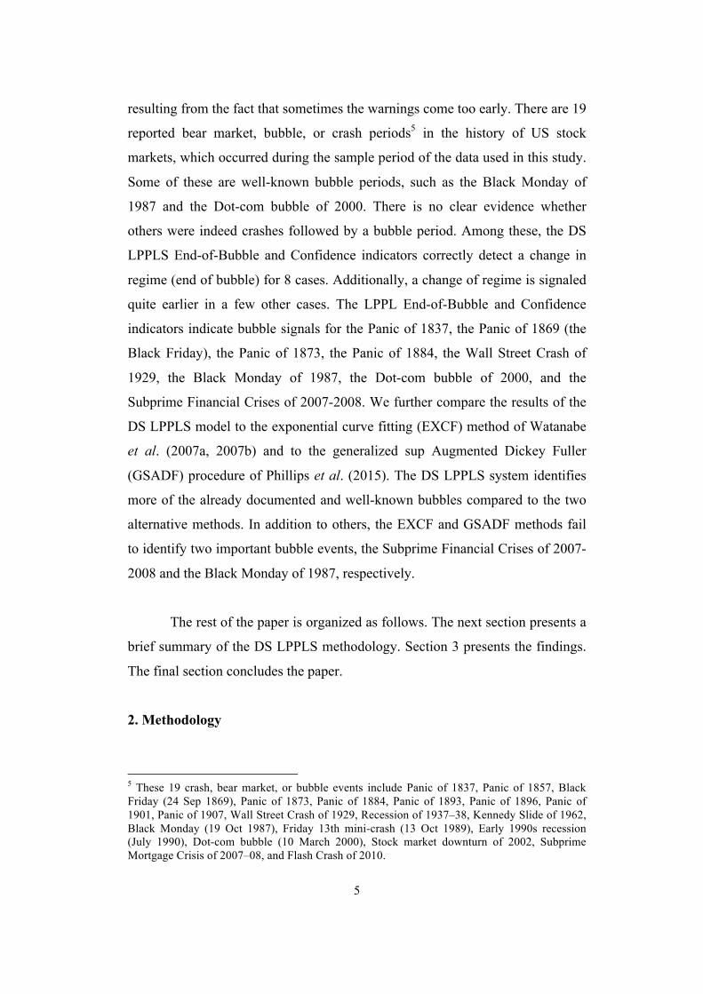
resulting from the fact that sometimes the warnings come too early. There are 19
reported bear market, bubble, or crash periods5 in the history of US stock
markets, which occurred during the sample period of the data used in this study.
Some of these are well-known bubble periods, such as the Black Monday of
1987 and the Dot-com bubble of 2000. There is no clear evidence whether
others were indeed crashes followed by a bubble period. Among these, the DS
LPPLS End-of-Bubble and Confidence indicators correctly detect a change in
regime (end of bubble) for 8 cases. Additionally, a change of regime is signaled
quite earlier in a few other cases. The LPPL End-of-Bubble and Confidence
indicators indicate bubble signals for the Panic of 1837, the Panic of 1869 (the
Black Friday), the Panic of 1873, the Panic of 1884, the Wall Street Crash of
1929, the Black Monday of 1987, the Dot-com bubble of 2000, and the
Subprime Financial Crises of 2007-2008. We further compare the results of the
DS LPPLS model to the exponential curve fitting (EXCF) method of Watanabe
et al. (2007a, 2007b) and to the generalized sup Augmented Dickey Fuller
(GSADF) procedure of Phillips et al. (2015). The DS LPPLS system identifies
more of the already documented and well-known bubbles compared to the two
alternative methods. In addition to others, the EXCF and GSADF methods fail
to identify two important bubble events, the Subprime Financial Crises of 2007-
2008 and the Black Monday of 1987, respectively.
The rest of the paper is organized as follows. The next section presents a
brief summary of the DS LPPLS methodology. Section 3 presents the findings.
The final section concludes the paper.
2. Methodology
5 These 19 crash, bear market, or bubble events include Panic of 1837, Panic of 1857, Black Friday (24 Sep 1869), Panic of 1873, Panic of 1884, Panic of 1893, Panic of 1896, Panic of 1901, Panic of 1907, Wall Street Crash of 1929, Recession of 1937–38, Kennedy Slide of 1962, Black Monday (19 Oct 1987), Friday 13th mini-crash (13 Oct 1989), Early 1990s recession (July 1990), Dot-com bubble (10 March 2000), Stock market downturn of 2002, Subprime Mortgage Crisis of 2007–08, and Flash Crash of 2010.

6
In this section, we recall the derivation of the log-periodic power law singularity
(LPPLS) model. This presentation of the LPPLS is based on JLS (2000). JLS
(2000) consider a risk neutral rational agent with rational expectations. This
implies an asset price p(t) following a martingale process. In market
equilibrium, there is equality between asset price and its conditional expectation
given all information available up to time t. This is a necessary condition for no
arbitrage. Assume that tc is the unknown crash or end of bubble time, also called
the critical time, with a probability density function q(t), a cumulative
distribution function Q(t) and hazard rate )](1/[)()( tQtqth −= . As it is well-
known, the hazard rate gives the probability of a crash in the next time period
given that it has not occurred yet. Let )1,0(∈k denote the fixed percentage by
which the price falls during a crash. Then the asset price dynamics can be
described as follows:
dp = µ(t)p(t)dt − kp(t)dj +σ (t)p(t)dW ⇒E[dp] = µ(t)p(t)dt − kp(t)[0+ h(t)dt] = µ(t)p(t)dt − kp(t)h(t)dt
(1)
where dW is the infinitesimal increment of the Wiener process with 0 mean and
variance equal to dt. The term dj denotes a discontinuous jump with j = 0
before the crash and j =1 after the crash occurs. The equations of no arbitrage
and rational expectations imply that 0][ =dpE , yielding )()( tkht =µ . Then the
asset price dynamics before the crash occurs is given by the differential equation
E[d ln p(t)) = kh(t)dt with the following solution:
E ln p(t)p(t0 )
⎡
⎣⎢
⎤
⎦⎥
⎡
⎣⎢⎢
⎤
⎦⎥⎥=κ h( ′t )d ′t
t0
t
∫ (2)
As also remarked by Blanchard (1979), the higher the probability of a
crash, the faster is the growth of the asset price in order to compensate investors
for the increased risk of a crash. JLS (2000) further assumes that a power law
describes the behavior of the variables close to a critical point and γκκχ −−≈ )( cA describes susceptibility of the diverging system where A is a

7
positive constant and γ is the positive critical exponent of susceptibility. See
Seyrich and Sornette (2016) for a recent micro-foundation. The susceptibility
quantifies the degree of sensitivity of a system to external perturbation. It is the
probability that a group of agents will have the same state given externals
influences in the network. In real financial markets, interacting investors are
organized inside a hierarchical network, where people locally influence each
other at many different levels. Therefore, JLS (2000) proposed a Hierarchical
Diamond Lattice (HDL) in order to represent this aspect of reality in financial
markets. In the structure of HDL after n iterations there will be
)42)(3/2( nN += agents and nL 4= links among them. Derrida et al. (1983)
solved a version of the HDL. It is similar to the rational imitation model in a
random or regular network with one difference. Here the critical exponent of
susceptibility, γ , can be a complex number. Then, the following expression
gives the general expression of the power law singular behavior:
…++−−′+−′≈ −− ])ln(cos[)()( 10 ψκκωκκκκχ γγccc AA (3)
where 0A , 1A and ω are real numbers. The oscillations called “log-periodic”
correct the pure power law singularity and reflects the underlying approximate
discrete scale invariance of the financial price dynamics (Sornette, 1998b). The
oscillations are periodic in ln(κc −κ ) and ω is their angular log-frequency
quantifying how the local period of the oscillations shrinks to zero as the critical
time of crash is reached. κ is a positive constant governing the tendency of
imitation among agents, the order in which network increases with κ . cκ is the
critical point determining the separation of different regimes. See Geraskin and
Fantazzini (2013) for further discussion of the relationship between κ and cκ
and the assumption that κ is locally linear in time. Within this mechanism, the
behavior of the crash hazard rate is similar to that of susceptibility in the
neighborhood of the critical crash point. We can then write the hazard rate as
follows:

8
])ln(cos[)()()( 10 ψωαα ′+−−+−≈ −− ttttBttBth ccc (4)
This expression shows that the hazard rate increases as the interactions among
investors rise with time. Appling this hazard rate to the solution of asset price
dynamics given by equation (2), we obtain the following equation which
describes the evolution of the asset price before a crash, which is known as the
Log Periodic Power Law singularity (LPPLS) formula:
ln[p(t)] ≈ A+B(tc − t)β{1+C cos[ω ln(tc − t)+φ] (5)
where 0))ln(p( >= ctA and B <0 for a positive bubble. C quantifies the size of
the log-periodic oscillations around the power law singular growth. β is positive
and less than unity. It quantifies the power law acceleration of asset prices. A
positive β ensures a finite asset price at the critical time ct of crash. The angular
log-frequency of oscillations during the bubble is denoted by ω. φ denotes the
phase parameter, which is positive and less than 2π. These parameters are
further described in Sornette and Johansen (2001) and Johansen (2003). The
LPPLS formula (5) is the main equation describing the evolution of asset prices
before a crash. This equation is given in various forms in several papers:
Sornette (2003b), Lin et al. (2014), and Geraskin and Fantazzini (2013).
For both developed and emerging stock markets, Johansen et al. (1999),
Johansen and Sornette (1999a), and Sornette and Johansen (2001) have
documented that the most speculative bubbles have two common characteristics.
First, a faster than exponential or super-exponential growth of the stock price
during the bubble period, which ends when the bubble fades. This super-
exponential growth can be characterized by the power law singularity of the
LPPLS model. Second, oscillations with an accelerating frequency that can be
represented as approximately in geometrical proportional to the distance to the
critical time tc (the most probable time for a regime change or end of bubble).

9
The structure of the LPPLS model in equation (5) describes these features. The
parameter tc is the most probable time for a change in the regime at which the
growth rate changes, signifying a change in regime. The regime change may be
the time of the crash, the burst of the bubble, or the fading of the bubble. Not all
bubbles end with a crash and therefore the change in regime is not necessarily a
crash. The regime change, however, will be a change from super-exponential
growth to a lower growth and the end of the accelerating oscillations. The first
component, A+B(tc − t)β , of the LPPLS model in equation (5) captures the
super-exponential growth. Therefore, this component is the power law singular
component. It is the component that embodies the positive feedback mechanism
of a bubble development. For super-exponential growth, it is required that
0 < β <1 , while positive and negative bubbles are characterized by B < 0 and
B > 0 , respectively. The sign requirements on B arise from the condition that
prices should rise during a positive bubble and fall during a negative bubble.
Positivity of the prices requires A > 0 .
Replacing tc − t with t − tc in equation (5) gives a price dynamics that
characterizes what is called an “anti-bubble” (Johansen and Sornette, 1999b;
Zhou and Sornette, 2004; 2005). The second component, C(tc − t)β describes
the fact that the amplitude of the accelerating oscillations drop to zero at the
critical time tc with additional requirements to guarantee a positive hazard rate
(Bothmer and Meister, 2003). In the LPPLS model, the term ω ln(tc − t)models
the fact that the local frequency of oscillations becomes infinite at the critical
time tc . It is in general required that 6 ≤ω ≤13 so that the log-periodic
oscillations to be neither too fast (fitting to the random component of the data),
nor too slow (providing a contribution to the trend). Finally, φ in equation (5) is
associated with a characteristic time units for the oscillations.
The LPPLS equation (5) has 3 linear parameters ( A,B,C ) and 4
nonlinear parameters (β,ω, tc,φ ). In order to simplify the estimation, usually 3
linear parameters A,B,C are “slaved” in the fitting algorithm and estimated

10
from the given values of the nonlinear parameters β,ω, tc , and φ (see, e.g.,
Johansen et al., 1999). A common method of estimation for the LPPLS
equation (5) is the nonlinear least squares. However, minimization of nonlinear
multivariate least squares functions is non-trivial due to presence of multiple
local minima, where the well-studied algorithms, such as the steepest descent or
the Newton’s method, usually will get trapped. In order to overcome to
complexity of the minimization, metaheuristic algorithms such as the taboo
search or genetic algorithm is used to estimate the parameters of the LPPL
model. Filimonov and Sornette (2013) proposed transforming the LLPLS
equation (5) in order to reduce the number of nonlinear parameters from 4 to 3
at the expense of increasing the number of linear parameters from 3 to 4. The
transformation substantially reduces the complexity of the fitting procedure and
improves its stability, allowing the simple algorithms, such as the Gauss-
Newton algorithm, to be used efficiently. The transformed function is
characterized by better smooth properties and in general by a single or a few
minima. This study also uses the procedure of Filimonov and Sornette (2013) in
order to estimate the parameters of the LPPLS model.
3. Data and Empirical Results
3.1. The DS LPPLS bubble identification
We collected monthly data on the Standard and Poor’s S&P 500 (S&P500)
stock market index from August 1791 through August 2014 for 2677
observations. Data come from the Global Financial Database. The LPPLS model
is estimated with a 269 month rolling window.
We define two targets for our investigation: positive bubbles and
negative bubbles. A positive bubble is an ascending accelerating (transient
super-exponential) price ending at some future critical time 𝑡!. A negative
bubble is the mirror image of a positive bubble under a flip of the vertical price
axis, and thus characterizes an accelerating descending price ending at some
11
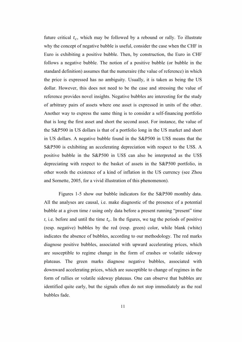
future critical 𝑡!, which may be followed by a rebound or rally. To illustrate
why the concept of negative bubble is useful, consider the case when the CHF in
Euro is exhibiting a positive bubble. Then, by construction, the Euro in CHF
follows a negative bubble. The notion of a positive bubble (or bubble in the
standard definition) assumes that the numeraire (the value of reference) in which
the price is expressed has no ambiguity. Usually, it is taken as being the US
dollar. However, this does not need to be the case and stressing the value of
reference provides novel insights. Negative bubbles are interesting for the study
of arbitrary pairs of assets where one asset is expressed in units of the other.
Another way to express the same thing is to consider a self-financing portfolio
that is long the first asset and short the second asset. For instance, the value of
the S&P500 in US dollars is that of a portfolio long in the US market and short
in US dollars. A negative bubble found in the S&P500 in US$ means that the
S&P500 is exhibiting an accelerating depreciation with respect to the US$. A
positive bubble in the S&P500 in US$ can also be interpreted as the US$
depreciating with respect to the basket of assets in the S&P500 portfolio, in
other words the existence of a kind of inflation in the US currency (see Zhou
and Sornette, 2005, for a vivid illustration of this phenomenon).
Figures 1-5 show our bubble indicators for the S&P500 monthly data.
All the analyses are causal, i.e. make diagnostic of the presence of a potential
bubble at a given time t using only data before a present running “present” time
t, i.e. before and until the time 𝑡!. In the figures, we tag the periods of positive
(resp. negative) bubbles by the red (resp. green) color, while blank (white)
indicates the absence of bubbles, according to our methodology. The red marks
diagnose positive bubbles, associated with upward accelerating prices, which
are susceptible to regime change in the form of crashes or volatile sideway
plateaus. The green marks diagnose negative bubbles, associated with
downward accelerating prices, which are susceptible to change of regimes in the
form of rallies or volatile sideway plateaus. One can observe that bubbles are
identified quite early, but the signals often do not stop immediately as the real
bubbles fade.

12
Figures 1-5 show the timeline of “DS LPPLS Bubble Status indicators”
of the S&P500 monthly data from January 1814 to August 2014. A DS LPPLS
Bubble Status indicator at any time t is constructed by looking for bubble
patterns in the 269 months before 𝑡! by calibrating the log-price time series with
the LPPLS model. If a portion of the 269 historic data points can be fitted by the
LPPLS model better than by an average exponential growth model, the status at
𝑡! is marked as either a positive bubble or a negative bubble, according to the
average positive versus negative trending price in the calibration window, with
red color or green color, respectively. The status of those periods that remain
blank (white) is no bubble.
—Insert Figure 1-5 here—
The DS LPPLS Bubble Status indicators in Figures 1-5 show the
possible periods where super-exponential growth is observed. The marked
periods do not all correspond to bubbles or negative bubbles. The DS LPPLS
Bubble Status indicators mark existence of possible bubbles for the well-known
19 bear market, bubble, or crash periods7 in the history of US stock markets,
which our study period covers. Although some of these events are classified as
known bubbles, there is no clear evidence on the status of the others. Among the
period outlined particularly by the DS LPPLS Bubble Status indicators in
Figures 1-5, the following one are known bubble events: the Black Friday of
1869, the Wall Stress Crash of 1929, the Black Monday of 1987, the Dot-com
bubble of 2000, and the Subprime Mortgage Crisis of 2007–08 are. These events
are listed in Table 1 along with some others that are classified as bubble. There
are some other periods where the DS LPPLS Bubble Status indicates the
possible existence of bubbles. We next examine the existence of bubbles in
these periods using robust indicators.
Table 1. The Events Classified as Bubble by the DS LPPLS System
The Event Description Change in the S&P500
7 See footnote 5 above.

13
and DS LPPL Confidence Value
The Panic of 18378 and the subsequent Six Year (1837-1843) Depression
The crisis was due to a period of sharply rising prices of land, cotton, and slaves from mid-1834 to mid-1836. It was followed by a sharp decline in these prices. The panic had both domestic and foreign origins, such as credit constraints imposed by the UK. The subsequent recession made profits, prices, and wages to go down and unemployment to raise.
The S&P index started to surge in 1830 and peaked to 3.6 in mid-1835. After then, the bubble burst and the index fell to 2.25 in 1837 and made a trough in 1843 at 1.6. The cumulative decline from June 1835 to March 1835 exceeded 50%. DS LPPLS Confidence value: 0.004
Black Friday, 24 Sep 1869
The United States Government issued a large amount of government debt, which were fiat greenbacks not backed by gold, during the reconstruction era following the Civil War. A group of speculators attempted to benefit from this. On September 20, 1869, the speculators started hoarding gold and caused the Black Friday.
The S&P index has risen more than 70% from April 1868 to September 1869. Following the Black Friday, the index fell by 7% in September 1869. DS LPPL Confidence value: 0.001
The Panic of 18739
The U.S. economy experienced an economic expansion between 1866-1873 due to heavy investment in transportation and protective tariffs. However, overproduction against a declining market, deflation, and the depression in Europe triggered a depression that lasted from 1873 until 1879. It is also called long depression or great depression.
The S&P index started to rise in 1866, and was a positive bubble between 1869-1873. Thereafter, the index started to fall until 1879, following a negative bubble. DS LPPL Confidence value: 0.008
Panic of 1884 The panic occurred during the Recession of 1882-85. The panic was caused by two bank failures having ripple effect across Wall Street causing many firms to fail. Speculative bonds and over extension of credit to fund the infrastructure construction, which caused a panic in 1882, also contributed to the panic of 1884.
The S&P index fell from 5.34 in Dec 1883 to 4.23 by the end of Dec 1884 with a cumulative decline of 25.26%. DS LPPL Confidence value: 0.002
The Great Depression (The Wall Street Crash of 1929)10
Speculation in stock market, production and/or sales fall in several manufacturing industries, high debts due to easy crediting, falling prices in some agricultural products and heavy emigration from rural to urban are listed as the causes of the great depression.
The S&P index started to surge in mid-1921 from 5.4 and peaked at 32 in 1929. Thereafter, the bubble burst and the index made a trough in mid-1932 by falling even below 5. DS LPPL Confidence value: 0.014
Black Monday, 19 Oct 1987
Black Monday refers to Monday, October 19, 1987, the day the major stock markets around the world crashed, with huge losses in a very short time. It started in Hong Kong and spread west to Europe, and later to the United States after other major markets of Europe declined significantly.
The S&P index fell exactly 70 points from September 1987 to October 1987 (24.54% decline). The cumulative decline in the S&P index exceeded 33% by the end of November
8 See Rousseau (2002). 9 See Barreyre (2011), Lubetkin (2006) and Coppock (1961) on the causes. 10 See Friedman and Schwarz (1963) for monetary-related, Bernanke (1983) for credit related, and Temin (1989) and Bernanke and James (1991) for gold-standard causes of the depression.
14
1987. DS LPPL Confidence value: 0.001
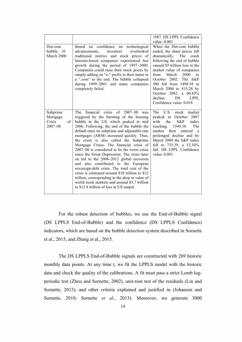
Dot-com bubble, 10 March 2000
Based on confidence on technological advancements, inventors overlooked traditional metrics and stock prices of Internet-based companies experienced fast growth during the period of 1997–2000. Companies could raise their stock prices by simply adding an “e-“ prefix to their name or a “.com” to the end. The bubble collapsed during 1999–2001 and many companies completely failed.
When the Dot-com bubble ended, the share prices fell dramatically. The crash following the end of bubble caused $5 trillion loss in the market value of companies from March 2000 to October 2002. The S&P 500 fell from 1498.58 in March 2000 to 815.28 by October 2002, a 60.85% decline. DS LPPL Confidence value: 0.018
Subprime Mortgage Crisis of 2007–08
The financial crisis of 2007–08 was triggered by the bursting of the housing bubble in the US, which peaked in mid 2006. Following, the end of the bubble the default rates on subprime and adjustable-rate mortgages (ARM) increased quickly. Thus, the crisis is also called the Subprime Mortgage Crises. The financial crisis of 2007–08 is considered to be the worst crisis since the Great Depression. The crisis later on led to the 2008–2012 global recession and also contributed to the European sovereign-debt crisis. The total cost of the crisis is estimated around $10 trillion to $12 trillion, corresponding to the drop in value of world stock markets and around $5.7 trillion to $12.8 trillion of loss in US output.
The U.S. stock market peaked in October 2007 with the S&P index reaching 1549.38. The market then entered a prolonged decline and by March 2009 the S&P index fell to 735.39, a 52.54% fall. DS LPPL Confidence value: 0.001.
For the robust detection of bubbles, we use the End-of-Bubble signal
(DS LPPLS End-of-Bubble) and the confidence (DS LPPLS Confidence)
indicators, which are based on the bubble detection system described in Sornette
et al., 2015, and Zhang et al., 2015.
The DS LPPLS End-of-Bubble signals are constructed with 269 historic
monthly data points. At any time t, we fit the LPPLS model with the historic
data and check the quality of the calibrations. A fit must pass a strict Lomb log-
periodic test (Zhou and Sornette, 2002), unit-root test of the residuals (Lin and
Sornette, 2013), and other criteria explained and justified in (Johansen and
Sornette, 2010; Sornette et al., 2013). Moreover, we generate 3000

15
bootstrapping samples by shuffling the residuals of the LPPLS fit, and check the
fraction of the samples that can pass the same strict tests, which gives the value
of the DS LPPLS Confidence indicator.
A DS LPPLS End-of-Bubble signal predicts that a bubble, either a
positive bubble or a negative bubble, is going to end. The corresponding DS
LPPLS Confidence indicator indicates the confidence level of the End-of-
Bubble signal. A higher value of a DS LPPLS Confidence indicator means that
the corresponding End-of-Bubble signal is more reliable. End-of-Bubble signals
of negative bubbles have negative DS LPPLS Confidence indicators. The DS
LPPLS Confidence indicator robustly marks bubbles by measuring the
sensitivity of the observed bubble pattern to the chosen starting time. If the
pattern exists only in a few of the analyzed windows, the value of the DS
LPPLS Confidence indicator will be close to zero. A DS LPPLS Confidence
value close to one means that the bubble pattern shows almost no sensitivity to
the choice of the data window. A very low value indicates risk of over-fitting
since the signal is only observed in one or two specific windows. In this case,
the result needs to be considered with care.
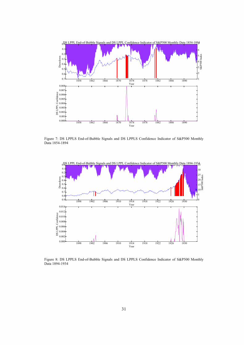
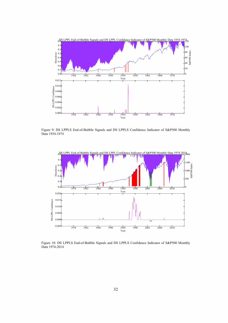
Figures 6-10 show the timeline of “DS LPPLS End-of-Bubble” signals
and “DS LPPLS Confidence” indicators of the S&P500 monthly data from
January 1814 to August 2014. The purple shades in the upper graphs depict the
drawdowns of the S&P500 monthly data.11 There are two times, 1842-1843 and
2002-2003, for which the End-of-Bubble signals of negative bubbles
successfully predict more than 30% rebounds, and our methods identify only
those two clusters of End-of-Bubble signals of negative bubbles. The End-of-
Bubble signals of positive bubbles, however, are able to predict a large fraction
11 Johansen and Sornette (1998, 2001) developed a methodology to characterize drawdowns (drawups) robustly. Drawdowns (drawups) were simply defined as a continuous decrease (increase) in the value of the price, while allowing for small noise decorating the main trend. A drawdown (drawup) is terminated by a sufficiently large increase (decrease) in the price. Drawdowns (drawups) are thus robust cumulative losses (gains) from the last local maximum (minimum) to the next minimum (maximum).

16
of the big drawdowns that develop in their future, with only two or three false
alarms, resulting from the fact that sometimes the warnings come too early.
—Insert Figure 6-10 here—
The DS LPPLS End-of-Bubble and Confidence indicators accurately
signal a change in regime (end of bubble) for 8 cases. All these are positive
bubble cases. Additionally, the DS LPPLS End-of-Bubble and Confidence
indicators indicate two negative bubbles. The positive bubbles signals
correspond to following events: the Panic of 1837, the Panic of 1869 (the Black
Friday), the Panic of 1873, the Panic of 1884, the Wall Street Crash of 1929, the
Black Monday of 1987, the Dot-com bubble of 2000, and the Subprime
Financial Crises of 2007-2008. Although other events have been well-
documented as bubbles before and have been studied using bubble detection
methodologies, to the best of our knowledge, the evidence for bubble presented
here for the Panic of 1837, the Panic of 1873, and the Panic of 1884 is novel.
Therefore, our present study presents for the first time solid statistical evidence
of bubbles for these cases. The description of these events and values of the DS
LPPLS Confidence are given in Table 1. The highest three values of the DS
LPPLS Confidence are estimated for the Dot-com bubble of 2000 (0.018), the
Crash of 1929 (0.014), and the Panic of 1873 (0.008). Thus, the bubble
confidence for the Panic of 1873 is considerably high. The DS LPPLS
Confidence estimates are around 0.001 for the Black Friday of 1869, the Black
Monday of 1987, and the Subprime Mortgage Crises of 2007-08. The DS
LPPLS Confidence estimates are 0.002 and 0.004, respectively, for the Panic of
1837 and the Panic of 1884.
In most cases, the DS LPPLS Confidence estimates give bubble signals
quite early before the end of the bubble period. The Panic of 1837 is signaled as
early as 1833, the Panic of 1884 as early as 1881-82, the Crash of 1929 as early
as 1927, and the Black Monday of 1987 as early as 1986. However, the signal
comes relatively late and weak for the Subprime Mortgage Crises of 2007-08.

17
Two negative bubbles in 1842-1843 and 2002-2003 correspond to the Six Year
Recession following the Panic of 1837 and Dot-com bubble of 2000,
respectively. Therefore, the negative bubbles also corresponds to known well-
documented events.. There are, however, three bubble signals in 1903, 1946,
1955 for which there are no recorded events for these periods. The DS LPPLS
Confidence value for 1955 has considerable high value of 0.011 relative to the
other values observed. But one can observe clear change of regimes following
the peak of these signals, suggesting value for mitigating market risks when
using such indicators.
3.2. Comparison with other methods
In this section, we use two additional bubble identification methods in order to
compare the results obtained from the DS LPPLS methodology. In this way, we
can both compare the results and do a robustness check by using these
alternative methods. Two methods we use for confirmatory and comparative
analysis are the exponential curve fitting (EXCF) method of Watanabe et al.
(2007a, 2007b) and the generalized sup augmented Dickey Fuller (GSADF)
procedure of Phillips et al. (2015).
The EXCF is based on the idea that an exponential growth curve fits
better than a linear model to bubble periods. The EXCF method determines a
data based window size to date-stamp the bubbles and crashes automatically.
The window size is determined such that exponential growth would not be
observed when an exponential curve is fitted to the data covering a sample size
larger than this minimum window size. Balcilar et al. (2014) and Deviren et al.
(2014) use the EXCF method to identify bubbles in exchange rates and oil
prices. The EXCF method is based on fitting the following exponential curve:
p(t)− p(t −1) = ω1(i;Ti )−1( ) p(t −1)− p0 (i;Ti )⎡⎣ ⎤⎦+ f (t) (6)

18
where p(t) is the price at time t , 1( ; )ii Tω is the parameter that characterize the
exponential growth behaviors in the i-th period of length iT (window size or
time scale), and f (t) is the error term. The case 1( ; ) 1ii Tω = characterizes the
random walk behavior and in this case p0 (i;Ti ) does not have any specific role.
For 1( ; ) 1ii Tω > , we have either exponentially increasing (bubble) or decreasing
(crash) price behavior and );(0 iTiP gives the base line of the exponential
divergence. The case 1( ; ) 1ii Tω < characterizes prices that are convergent to
p0 (i;Ti ) .
In order to identify the bubble periods, the parameters );(1 iTiω and p0 (i;Ti )
are uniquely estimated from the past iT data points by minimizing the root mean
square error. In order to determine the window size iT , we first fit an
autoregressive model of order 4, AR(4), to the monthly S&P500 data.12 Then,
we simulate synthetic price data from the fitted AR(4) by changing the window
size from 20 to 400. The value for iT is estimated as the minimum window size
for which ω1(i;Ti ) ≤1 always holds. With 2000 Monte Carlo simulations, we
find that a window size of 100 is sufficient for the monthly S&P500 data.
Once the minimum window size is determined, a rolling estimation
procedure is used to determine the bubble periods.13 The procedure involves the
following steps: (i): );(1 iTiω and p0 (i;Ti ) are estimated by fitting equation (6)
over the past iT steps, and if 1( ; ) 1ii Tω > , all time steps in the observing box of
12 The order of the AR model is determined by the Bayesian Information Criterion (BIC). 13 The rolling estimation of the parameter ω1(i;Ti ) does not assume any parameter stability. This approach, given the optimal minimum window size, tracks the changes in ω1(i;Ti ) .

19
size iT steps are assigned as exponentially divergent; and if 1( ; ) 1ii Tω ≤ only the
latest time step in the box is assigned as convergent; (ii) the box is shifted by
one step and (i) is repeated; and (iii) after all periods are assigned a divergent or
convergent status, neighboring divergent time steps are connected.
As the second method for confirmatory analysis, we make use the GSADF
test procedure of Phillips et al., (2015). The GSADF is a recursive right-tailed
unit root testing procedure that allows the identification of multiple periods of
price explosiveness. Here, following the suggestions of Phillips et al., (2015),
we use a window-size of 36. This method uses a flexible moving sample test
procedure to consistently and efficiently detect and date-stamp periods where a
price series displays a root exceeding unity. The GASDF procedure is
implemented by testing a unit root against a right sided alternative using a
fraction rw of the sample, or a window size of Tw = [rwT ] , where [⋅] means the
integer part. Then, a backward sup ADF test is used with a varying window size
rw = r2 − r0 , where the end point of the subsample remains fixed at a fraction r2
of the entire sample, with the window size expanding from an initial fraction r0
to r2 , and the sup of all such backward ADF tests are taken. In the GASDF test,
the backward sup ADF is repeatedly implemented for each r2 ∈ [r0,1] and sup of
all such tests gives the final test value. Phillips et al. (2013) show that the
GSADF test has efficient bubble detection capabilities even in the presence of
multiple bubble episodes.
The bubble periods identified by the EXCF method and the GSADF test
are given in Table 2. We first comment on the results from the EXCF model.
The EXCF procedure identifies 14 bubble periods over the whole sample period.
Among the 14 bubble periods, five corresponds to historically known and
documented events as bubbles or crashes. These include the Panic of 1857, the
Panic of 1901, the Wall Street Crash of 1929, the Black Monday of 1987, and
the Dot-com bubble of 2000. The EXCF method also gives a very early signal

20
(two years ahead) for the Panic of 1837. According to the results summarized in
Table 1, the EXCF method has eight false signals in total.
The list of bubble periods identified by the GSADF test is also given in
Table 2. The GSADF test identifies 10 bubble periods, five of these
corresponding to known and documented events, one as an early signal (for the
panic of 1837 as early as 1835), and four false signals. The GASDF correctly
identifies the Panic of 1857, the Wall Street Crash of 1929, the Dot-com bubble
of 2000, the stock market downturn of 2002, and the Subprime Financial Crises
of 2007-2008.
Table 2. The Periods Determined as Bubbles by the Exponential Model and the GSADF Test
Bubble Periods Implied by the
Exponential Model Bubble Periods Implied by the
GSADF Test Nov 1814-Dec 1816 Jan 1835-Nov 1835† Jan 1842-Feb 1843 Jul 1857-Dec 1857* Feb 1864-Sep 1864 Feb 1877-Mar 1878 Jan 1881-Nov 1882 Feb 1901-Oct 1902* Dec 1925-Oct 1929* Apr 1932-Jul 1932
Apr 1954-Nov 1956 Oct 1964-Nov 1964 Feb 1986-Oct 1987* Nov 1995-Sep 2000*
May 1835-Jun 1835† Oct 1857-Nov 1857* Mar 1877-Jul 1877
Nov 1928-Oct 1929* May 1932-Jun 1932 Sep 1974-Oct 1974
May 1997-Nov 2001* Feb 2002-Apr 2002* May 2007-Jun 2007* Feb 2009-Mar 2009
* Periods corresponding to known and documented historical bubbles or crashes. † Periods that precede to known and documented historical bubbles or crashes.
—Insert Figure 11-12 here—
When we compare the results of the EXCF model and of the GSADF
test with the results of the DS LPPLS system, both the DS LPPLS and EXCF
methods identify the same five bubbles while five bubbles are also jointly

21
identified by both the DS LPPLS system and the GSADF test. Four bubbles, the
Panic of 1837, the Panic of 1857, the Wall Street Crash of 1929, and the Dot-
com bubble of 2000, are identified jointly by all three methods. Among the
important historical events, the GSADF test fails to identify the Black Monday
of 1987 while the EXCF method fails to identify the Subprime Financial Crises
of 2007-2008. In sum, among the eight bubbles identified by the DS LPPLS
system, the six events are also identified as bubbles by the EXCF and GSADF
methods. Four of these six bubbles are identified by both the EXCF and GSADF
methods, while each method additionally identifies one bubble period that are
also identified as bubble by the DS LPPL system. We also note that the EXCF
and GSADF methods cannot identify negative bubbles. The DS LPPLS system
also identifies previously unclassified bubble regimes, which are clearly
associated with significant changes of regimes, providing additional value for a
global riks management perspective. Overall, the DS LPPLS system accurately
identifies more of the historically events that are known as bubbles and has
fever (or no) false signals (if one recognizes the value of the regime-switching
identification). Among the three methods, the EXCF seem to give more frequent
false bubble signals while the GSADF method diagnoses fewer bubbles than
really exist.
4. Conclusion
In this study, we apply the LPPLS methodology introduced by Sornette et al.
(1996) and Sornette and Johansen (1997, 1998), on monthly S&P500 stock
prices in order to identify bubbles and crashes in the US stock market using two
centuries of data from 1814 to 2014. The distinguishing feature of this study
from the previous studies is that this paper is the first of its kind that examines
the existence of bubbles in the US stock prices using two hundreds years of
monthly data with an advanced bubble detection methodology based on the
LPPLS model. We found eight periods of positive bubbles in the S&P500 and
two periods of negative bubbles in the period from January 1814 to August
2014. Our analyses showed that the S&P500 experienced positive bubbles in the

22
following eight periods: the Panic of 1837, the Panic of 1869 (the Black Friday),
the Panic of 1873, the Panic of 1884, the Wall Street Crash of 1929, the Black
Monday of 1987, the Dot-com bubble of 2000, and the Subprime Financial
Crises of 2007-2008. We showed that each of these bubble periods correspond
to well-known and well-documented historical events, implying that the
detection algorithm indeed accurately detect the bubbles. To the best of our
knowledge, three of the bubble periods, the Panic of 1837, the Panic of 1873,
and the Panic of 1884, that our methodology detects correspond to well-known
events, but not studied in the literature using bubble detection methodologies.
Two negative bubbles detected by our methodology do also correspond to
known events. Thus the bubble indicators for these events are also correct
signals.
Our study shows that, among the 19 events documented as bear market,
crash, or the bubble in the history of the US stock market between 1814 and
2014, only eight events can be classified as positive bubbles with positive
feedback mechanism. Additionally two events are classified as negative
bubbles. These bubbles and crashes in the stock market, triggered by various
reasons, all developed a positive (or negative in two cases) feedback
mechanism, a self-perpetuating pattern of investment behavior. The positive
(negative) feedback mechanism translates into super-exponential growth
(decline) in stock prices. However, not all stock market crashed or crises are
caused by internal bubble mechanisms with positive (negative) feedback
mechanism. Some of these events are not preceded by faster than exponential
price growths (declines) and the crashes are caused by various economic and
political events, such as the recessions, panics, wars, end external influences.
We performed a confirmatory and comparative analysis using two
alternative methods. Combined together, the EXCF and the GSADF methods do
also identify six of the eight periods as bubbles, which were classified as
bubbles by the DS LPPLS system. Both the EXCF and the GSADF methods fail
to identify two well-known and well-documented bubbles. The Black Monday

23
of 1987 and the Subprime Financial Crises of 2007-2008 are not identified as
bubbles by the GSADF and EXCF methods, respectively. We also find that the
GSADF method tends to signal fewer bubbles than the other two methods, while
the EXCF method has the tendency to falsely detect too may bubbles. Both the
GSADF and the EXCF methods do not identify negative bubbles and give
higher number of false signals compared to the DS LPPLS method.
Our study shows that, with frequently occurring influential events in the last
two centuries of the history of the US stock market, regime shifts, and change of
regimes are the “norm” rather than the exception. The actors and policy makers
should well be aware that that these regime shifts and change of regimes are
likely to occur more frequently in the future (Sornette and Cauwels, 2014;
2015). Based on robust statistical evidence and a two hundreds years long
monthly time series data, our study highlights that financial markets exhibit
transitions between phases of growth, exuberance and crises (Lera and Sornette,
2015). Not all but most crises are endogenous and are the consequence of
procyclical positive or negative feedbacks that eventually burst (Johansen and
Sornette, 2010). Our study also shows that it possible to detect crashes ahead of
time and reduce the welfare loss arising from these. The study underlines the
importance a dynamical time at risk management (Kovalenko and Sornette,
2013) and its possibility, based on a sound monitoring system and scenario
analysis that is capable of recognizing the ubiquitous of positive and negative
feedbacks.

24
References
Balcilar, M, Ozdemir, Z., and Yetkiner, I. 2014. Are there really bubbles in oil prices? Physica A 416, p. 631-638.
Barreyre, N. 2011. The Politics of Economic Crises: The Panic of 1873, the
End of Reconstruction, and the Realignment of American Politics. The Journal of the Gilded Age and Progressive Era 10, 403-423.
Bernanke, B.S. 1983. Non-Monetary Effects of the Financial Crisis in the Propagation of the Great Depression. The American Economic Review 73, 257-276.
Bernanke, B.S., James, H. 1991. The Gold Standard, Deflation, and Financial Crisis in the Great Depression: An International Comparison. In: R. Glenn Hubbard, Ed., Financial Markets and Financial Crises, 33-68, Chicago & New York: University of Chicago Press.
Blanchard, O.J. 1979. Speculative bubbles, crashes and rational expectations. Economics Letters 3, 387-389.
Bothmer, H.C.G. and Meister, C., 2003. Predicting critical crashes? A new restriction for the free variables. Physica A 320, 320, 539-547.
Coppock, D. J. 1961. The Causes of the Great Depression, 1873-96. The Manchester School 29, 205-32.
Derrida, B., De Seze, L., Itzykson, C. 1983. Fractal structure of zeros in hierarchical models. Journal of Statistical Physics 33, 559-569.
Deviren, B, Kocakaplan, Y., Keskin, M., Balcılar, M., Özdemir, Z.A., Ersoy, E. 2014. Analysis of bubbles and crashes in the TRY/USD, TRY/EUR, TRY/JPY and TRY/CHF exchange rate within the scope of econophysics. Physica A 410, 414-420.
Filimonov, V., Sornette, D. 2013. A stable and robust calibration scheme of the
log-periodic power law model, Physica A 392, 3698-3707.
Friedman, M., Schwartz, A. J. 1963. Monetary History of the United States 1867-1960. Princeton: Princeton University Press.
Geraskin, P., Fantazzini, D. 2013. Everything you always wanted to know about log-periodic power laws for bubble modeling but were afraid to ask. The European Journal of Finance 19, 366-39.
Hüsler, A., D. Sornette and C. H. Hommes, 2013. Super-exponential bubbles in lab experiments: evidence for anchoring over-optimistic expectations on price, Journal Economic Behavior and Organization 92, 304-316.

25
Jiang, Z., Zhou, W.-X., Sornette, D., Woodard, R., Bastiaenseng, K., Cauwels, P. 2010. Bubble Diagnosis and Prediction of the 2005-2007 and 2008-2009 Chinese Stock Market Bubbles. Journal of Economic Behavior & Organization 74, 149–162.
Johansen, A. 2003. Characterization of large price variations in financial markets. Physica A 324, 157-166.
Johansen, A., Sornette, D. 1998. Stock market crashes are outliers. European Physical Journal B 1, 141-143.
Johansen, A., Sornette, D. 1999a. Critical crashes. Risk 12, 91–94.
Johansen, A. and D. Sornette, 1999b. Financial “anti-bubbles”: log-periodicity in Gold and Nikkei collapses, Int. J. Mod. Phys. C 10(4), 563-575.
Johansen, A., Sornette, D. 2000. Evaluation of the Quantitative Prediction of a Trend Reversal on the Japanese Stock Market in 1999. International Journal of Modern Physics C 11, 359-364.
Johansen, A. and D. Sornette, 2001/02. Large Stock Market Price Drawdowns Are Outliers, Journal of Risk 4(2), 69-110.
Johansen A., Sornette, D. 2010. Shocks, Crashes and Bubbles in Financial Markets. Brussels Economic Review (Cahiers economiques de Bruxelles) 53, 201-253.
Johansen, A., Ledoit, O., Sornette, D. 2000. Crashes as critical points. International Journal of Theoretical and Applied Finance 3, 219–255.
Johansen, A., Sornette, D., Ledoit, O. 1999. Predicting financial crashes using discrete scale invariance. Journal of Risk 1, 5–32.
Kovalenko, T. and D. Sornette, 2013. Dynamical Diagnosis and Solutions for Resilient Natural and Social Systems, Planet@ Risk 1 (1), 7-33, Davos, Global Risk Forum (GRF).
Leiss, M., H.H. Nax and D. Sornette, 2015. Super-Exponential Growth Expectations and the Global Financial Crisis, Journal of Economic Dynamics and Control 55, 1-13.
Lera, S. and D. Sornette, 2015. Secular bipolar growth rate of the real US GDP per capita: implications for understanding past and future economic growth, ETH Zurich preprint (http://ssrn.com/abstract=2703882)
Lin, L., Sornette, D. 2013. Diagnostics of Rational Expectation Financial Bubbles with Stochastic Mean-Reverting Termination Times. The European Journal of Finance 19, 344-365.

26
Lin, L., Ren, R., Sornette, D. 2014. The Volatility-Confined LPPL Model: A Consistent Model of ‘Explosive’ Financial Bubbles With Mean-Reversing Residuals, International Review of Financial Analysis 33, 210-225.
Lubetkin, M.J. 2006. Jay Cooke's Gamble: The Northern Pacific Railroad, the Sioux, and the Panic of 1873, Norman: University of Oklahoma Press.
Phillips, P.C.B., Shi, S-P., and Yu, J. (2015). Testing for Multiple Bubbles: Historical Episodes of Exuberance and Collapse in the S&P 500, International Economic Review, 2015, 56 (4 ), 1043-1078.
Rousseau, P. L. 2002. Jacksonian Monetary Policy, Specie Flows, and The Panic of 1837. The Journal of Economic History 62, 457-488.
Seyrich, M. and D. Sornette, 2016. Micro-foundation using percolation theory of the finite-time singular behavior of the crash hazard rate in a class of rational expectation bubbles, Int. J. Mod. Phys. C (submitted 28 Jan. 2016) (http://ssrn.com/abstract=2722383)
Sornette, D. 1998a. Large Deviations and Portfolio Optimization. Physica A 256, 251-283.
Sornette, D. 1998b. Discrete scale invariance and complex dimensions, Physics Reports 297, Issue 5, 239-270 (extended version at http://xxx.lanl.gov/abs/cond-mat/9707012)
Sornette, D. 2003a. Critical Market Crashes. Physics Reports 378, 1–98.
Sornette, D. 2003b. Why Stock Markets Crash (Critical Events in Complex Financial Systems). Princeton: Princeton University Press.
Sornette, D. and P. Cauwels, 2014. 1980-2008: The Illusion of the Perpetual Money Machine and what it bodes for the future, Risks 2, 103-131.
Sornette, D. and P. Cauwels, 2015. Managing risks in a creepy world, Journal of Risk Management in Financial Institutions (JRMFI) 8 (1), 83-108.
Sornette, D., G. Demos, Q. Zhang, P. Cauwels, V. Filimonov and Q.Zhang, 2015. Real-time prediction and post-mortem analysis of the Shanghai 2015 stock market bubble and crash, Journal of Investment Strategies 4 (4), 77-95 (2015).
Sornette, D., Johansen, A. 1997. Large Financial Crashes. Physica A 245, 411-422.
Sornette, D., Johansen, A. 1998. A Hierarchical Model of Financial Crashes. Physica A 261, 581-598.

27
Sornette, D., Johansen, A. 2001. Significance of log-periodic precursors to financial crashes. Quantitative Finance 1, 452-471.
Sornette, D., Johansen, A., Bouchaud, J.P. 1996. Stock Market Crashes, Precursors and Replicas. J. Phys. I France 6, 167-175.
Sornette, D., Woodard, R., Zhou, W.-X. 2009. The 2006-2008 Oil Bubble: Evidence of Speculation, and Prediction. Physica A 388, 1571-1576.
Sornette, D., Woodard, R., Yan, W., Zhou, W.-X. 2013. Clarifications to Questions and Criticisms on the Johansen-Ledoit-Sornette bubble Model, Physica A 392, 4417-4428.
Sornette, D., Zhou, W.-X. 2006. Predictability of Large Future Changes in Major Financial Indices. International Journal of Forecasting 22, 153– 168.
Temin, P., 1989. Lessons from the Great Depression. Cambridge, Mass.: MIT Press.
Watanabe, K., Takayasu, H. , Takayasu M. 2007a. Extracting the Exponential Behaviors in the Market Data. Physica A 382, 336-39.
Watanabe, K., Takayasu, H. , Takayasu M. 2007b. A Mathematical Definition
of the Financial Bubbles and Crashes. Physica A. 383, 120-24. Yan, W., Rebib, R., Woodard, R., Sornette, D. 2012. Detection of Crashes and
Rebounds in Major Equity Markets. International Journal Portfolio Analysis and Management 1, 59–79.
Zhang, Q., Q. Zhang and D. Sornette, 2015. Early warning signals of financial crises with multi-scale quantile regressions of Log-Periodic Power Law Singularities, Int. J. Forecasting (submitted 14 Oct. 2015) (http://ssrn.com/abstract=2674128)
Zhou, W.-X., Sornette, D. 2002. Statistical Significance of Periodicity and Log-Periodicity with Heavy-Tailed Correlated Noise. Int. J. Mod. Phys. C 13, 137-170.
Zhou, W.-X., Sornette, D. 2003. Renormalization group analysis of the 2000-2002 anti-bubble in the US S&P 500 index: Explanation of the hierarchy of five crashes and prediction. Physica A 330, 584-604
Zhou, W.-X. and D. Sornette, 2004. Antibubble and Prediction of China's stock market and Real-Estate, Physica A, 337 (1-2), 243-268.
Zhou, W.-X. and D. Sornette, 2005. Testing the Stability of the 2000-2003 US Stock Market “Antibubble”, Physica A 348, 428-452..

28
Figure 1: DS LPPLS Bubble Status of S&P500 Monthly Data 1814-1854
Figure 2: DS LPPLS Bubble Status of S&P500 Monthly Data 1854-1894

29
Figure 3: DS LPPLS Bubble Status of S&P500 Monthly Data 1894-1934
Figure 4: DS LPPLS Bubble Status of S&P500 Monthly Data 1934-1974

30
Figure 5: DS LPPLS Bubble Status of S&P500 Monthly Data 1974-2014
Figure 6: DS LPPLS End-of-Bubble Signals and DS LPPLS Confidence Indicator of S&P500 Monthly Data 1814-1854
31
Figure 7: DS LPPLS End-of-Bubble Signals and DS LPPLS Confidence Indicator of S&P500 Monthly Data 1854-1894
Figure 8: DS LPPLS End-of-Bubble Signals and DS LPPLS Confidence Indicator of S&P500 Monthly Data 1894-1934
32
Figure 9: DS LPPLS End-of-Bubble Signals and DS LPPLS Confidence Indicator of S&P500 Monthly Data 1934-1974
Figure 10: DS LPPLS End-of-Bubble Signals and DS LPPLS Confidence Indicator of S&P500 Monthly Data 1974-2014
Top Related