


Languages
Pages
Legal

Low-Rank and Sparse Matrix Decomposition for Accelerated Dynamic MRI
with Separation of Background and Dynamic Components
Ricardo Otazo1, Emmanuel Candès2, Daniel K. Sodickson1
1Department of Radiology, NYU School of Medicine, New York, NY, USA
2Departments of Mathematics and Statistics, Stanford University, Stanford, CA, USA
Corresponding author: Ricardo Otazo, Bernard and Irene Schwartz Center for Biomedical
Imaging, Department of Radiology, New York University School of Medicine, 660 First Ave, 4th
Floor, New York, NY, USA. Phone: 212-263-4842. Fax: 212-263-7541. Email:
Running title: L+S reconstruction
Keywords: compressed sensing, low-rank matrix completion, sparsity, dynamic MRI
Word count of the manuscript body: 4983.
Abstract
Purpose: To apply the low-rank plus sparse (L+S) matrix decomposition model to reconstruct
undersampled dynamic MRI as a superposition of background and dynamic components in
various problems of clinical interest.
Theory and Methods: The L+S model is natural to represent dynamic MRI data. Incoherence
between k-t space (acquisition) and the singular vectors of L and the sparse domain of S is
required to reconstruct undersampled data. Incoherence between L and S is required for robust
separation of background and dynamic components. Multicoil L+S reconstruction is formulated
using a convex optimization approach, where the nuclear-norm is used to enforce low-rank in L
and the l1-norm to enforce sparsity in S. Feasibility of the L+S reconstruction was tested in
several dynamic MRI experiments with true acceleration including cardiac perfusion, cardiac
cine, time-resolved angiography, abdominal and breast perfusion using Cartesian and radial
sampling.
Results: The L+S model increased compressibility of dynamic MRI data and thus enabled high
acceleration factors. The inherent background separation improved background suppression
performance compared to conventional data subtraction, which is sensitive to motion.
Conclusion: The high acceleration and background separation enabled by L+S promises to
enhance spatial and temporal resolution and to enable background suppression without the need
of subtraction or modeling.
Keywords: compressed sensing, low-rank matrix completion, sparsity, dynamic MRI
Introduction
The application of compressed sensing (CS) to increase imaging speed and efficiency in
MRI demonstrated great potential to overcome some of the major limitations of current
techniques in terms of spatial resolution, temporal resolution, volumetric coverage and
sensitivity to organ motion. CS exploits the fact that an image is sparse in some appropriate basis
to reconstruct undersampled data (below the Nyquist rate) without loss of image information (1-
3). Successful application of CS requires image sparsity and incoherence between the acquisition
space and representation space. MRI presents favorable conditions for the application of CS,
since (a) medical images are naturally compressible by using appropriate sparsifying transforms,
such as wavelets, finite differences (total variation), learned dictionaries (4) and many others,
and (b) MRI data are acquired in the spatial frequency domain (k-space) rather than in the image
domain, which facilitates the generation of incoherent aliasing artifacts via random
undersampling of Cartesian k-space or the use of non-Cartesian k-space trajectories. Image
reconstruction is performed by enforcing sparsity in the solution, which is usually accomplished
by minimizing the l1-norm in the sparse domain, subject to data consistency constraints. A key
advantage for MRI is that CS can be combined with parallel imaging to further increase imaging
speed by exploiting joint sparsity in the multicoil image ensemble rather than in each coil
separately (5-8). Dynamic MRI is particularly well suited for the application of CS, due to
extensive spatiotemporal correlations that result in sparser representations than would be
obtained by exploiting spatial correlations alone. (Similar observations account for the fact that
videos are generally far more compressible than static images).
The idea of compressed sensing for signal/image vectors can be extended to matrices
enabling recovery of missing or corrupted entries of a matrix under low-rank and incoherence
conditions (9). Just as sparse signals/images, which only have few large coefficients, depend
upon a smaller number of degrees of freedom, low-rank matrices with only a few large singular
values also depend on a small number of parameters. Low-rank matrix completion is performed
by minimizing the nuclear-norm of the matrix (sum of singular values), which is the analog of
the l1-norm for signal vectors (sum of absolute values), subject to data consistency constraints
(10). Low-rank matrix completion has been applied to dynamic MRI by considering each
temporal frame as a column of a space-time matrix, where the spatiotemporal correlations

produce a low-rank matrix (11,12). Local k-space correlations in a multicoil data set have been
exploited to perform calibrationless parallel imaging reconstruction via low-rank matrix
completion (13).
The combination of compressed sensing and low-rank matrix completion represents an
attractive proposition for further increases in imaging speed. In dynamic MRI, previous work on
this combination proposed finding a solution that is both low-rank and sparse (14,15). A different
model suggested decomposing a data matrix as a superposition of a low-rank component (L) and
a sparse component (S) (16,17). Whereas topics in graphical modeling motivate the L+S
decomposition in (17), the aim in (16) is quite different. The idea is to use the L+S
decomposition to perform robust principal component analysis (RPCA); that is to say, to recover
the principal components of a data matrix with missing or corrupted entries. RPCA improves the
performance of classical PCA in the presence of sparse outliers, which are captured in the sparse
component S. RPCA, or equivalently the L+S decomposition, has been successfully applied to
computer vision, where it enables separation of the background from the foreground in a video
sequence (16), to image alignment (18), and to image reconstruction in 4DCT with reduced
numbers of projections (19).
The L+S decomposition is particularly suitable for dynamic imaging, where L can model
the temporally correlated background and S can model the dynamic information that lies on top
of the background. Preliminary work on the application of L+S to dynamic MRI has been
reported by Gao et al. (20) to reconstruct retrospectively undersampled cardiac cine data sets and
to separate cardiac motion from a common background among frames. While this work
establishes a precedent in MRI, it is limited to retrospective undersampling in a single are of
application.
In this work, we extend the work Gao et al. (20) and present L+S reconstructions for
dynamic MRI using joint multicoil reconstruction for Cartesian and non-Cartesian k-space
sampling, show examples with true acceleration and introduce novel applications, such as
separation of contrast enhancement from background, and the ability to perform background
suppression without the need of subtraction or modeling. We also demonstrate the superior
compressibility of the L+S model compared to using a sparse model only. Reconstruction of
highly-accelerated dynamic MRI data corresponding to cardiac perfusion, cardiac cine, time-

resolved peripheral angiography, abdominal and breast perfusion using Cartesian and golden-
angle radial sampling are presented to show feasibility and general applicability of the L+S
method.

Theory
L+S matrix decomposition
The L+S approach aims to decompose a matrix M as a superposition of a low-rank matrix
M (few non-zero singular values) and a sparse matrix S (few non-zero entries). When such a
decomposition M = L+S exists, we would like it to be unique so that it makes sense to search for
the well-defined components L and S given that we only see their sum M (this is a sort of a blind
deconvolution/separation problem). It turns out that when the low-rank component is not sparse,
and vice versa, the sparse component does not have low rank, as would be the case when the
locations of its nonzero entries are sampled at random, the decomposition is unique and the
problem well posed (16,17). We refer to this condition as incoherence between L and S.
The L+S decomposition is performed by solving the following convex optimization
problem:
SLMtsSL +=+∗
.. min1
λ , (1)
where ∗
L is the nuclear norm or sum of singular values of the matrix L, 1S is the l1-norm or
sum of absolute values of the entries of S and λ is a tuning parameter that balances the
contribution of the l1-norm term relative to the nuclear norm term. This approach finds a unique
decomposition with extremely high probability, if L and S are sufficiently incoherent.
L+S representation of dynamic MRI
In analogy to video sequences and following the work of Gao et al. (20), dynamic MRI
can be inherently represented as a superposition of a background component and a dynamic
component. The background component corresponds to the highly correlated information among
frames, which is slowly changing over time. The dynamic component captures the innovation
introduced in each frame, which is rapidly changing over time and can be assumed to be sparse
since substantial differences between consecutive frames are usually limited to comparatively
small numbers of voxels. Our hypothesis is that the L+S decomposition can model dynamic MRI

data more efficiently than a low-rank or sparse model alone, or than a model in which both
constraints are enforced simultaneously.
To apply the L+S decomposition to dynamic MRI, the time-series of images is converted
to a matrix M, where each column is a temporal frame. The application of the L+S
decomposition will produce a matrix L that represents the background component and a matrix S
that corresponds to the innovation from column-to-column, e.g., organ motion or contrast-
enhancement. Figure 1 shows the L+S decomposition of cardiac cine and perfusion data sets,
where L captures the correlated background between frames and S captures the dynamic
information (heart motion for cine and contrast-enhancement for perfusion). Note that the L
component is not constant over time, but is rather slowly changing among frames, which differs
from just taking a temporal average. In fact, for the case of cardiac cine, the L component
includes periodic motion in the background, since it is highly correlated among frames.
Another important feature is that the S component has sparser representation than the
original matrix M, since the background has been suppressed. This gain in sparsity is already
obvious in the original y-t space, but it is more pronounced in an appropriate transform domain
where dynamic MRI is usually sparse, such as the temporal frequency domain (y-f) that results
from applying a Fourier transform along the columns of S. The rightmost column of Figure 1
shows the S component in the y-f domain for the cardiac cine and perfusion data sets mentioned
above. This increase in sparsity given by the background separation will in principle enable
higher acceleration factors, since fewer coefficients need to be recovered, if the load to represent
the low-rank component is lower. In order to test this hypothesis, the compressibility of dynamic
MRI data using L+S and S-only models were compared quantitatively on the cardiac cine and
perfusion data sets mentioned above using a temporal Fourier transform as the sparsifying
transform. Rate-distortion curves were computed using the root mean square error (RMSE) as
distortion metric (Figure 2). Data compression using the S-only model was performed by
discarding low-value coefficients in the transform domain according to the target compression
ratio, i.e. only the top n/C coefficients were used to represent the image, where n is the total
number of coefficients and C is the target compression ratio. Data compression using the L+S
model was performed by assuming a fixed low-rank approximation, e.g. rank(L) = 1, 2 or 3,
which was subtracted from the original matrix M to get S. S was then transformed to the sparse

domain and coefficients were discarded according to the target compression rate and the number
of coefficients to represent the L component, e.g. the top n/C-nL coefficients were used to
represent S, with nL coefficients used to represent L. nL is given by ( )ts nnLrank +×)( , where ns is
the number of spatial points and nt is the number of temporal points. The rate-distortion curves in
Figure 2 clearly show the advantages of the L+S model in representing dynamic MRI images
with fewer degrees of freedom, which will lead to higher acceleration or undersampling factors.
Incoherence requirements
L+S reconstruction of undersampled dynamic MRI data involves three different types of
incoherence:
• Incoherence between the acquisition space (k-t) and the representation space of the low-rank
component (L)
• Incoherence between the acquisition space (k-t) and the representation space of the sparse
component (S)
• Incoherence between L and S spaces, as defined earlier.
The first two types of incoherence are required to remove aliasing artifacts and the last
one is required for separation of background and dynamic components. The standard k-t
undersampling scheme used for compressed sensing dynamic MRI, which consists of different
variable-density k-space undersampling patterns selected in a random fashion for each time
point, can be used to meet the requirement for the first two types of incoherence. Note that in this
sampling scheme, low spatial frequencies are usually fully-sampled and the undersampling factor
increases as we move away from the center of k-space. First, high incoherence between k-t space
and L is achieved since the column space of L cannot be approximated by a randomly selected
subset of high spatial frequency Fourier modes and the row-space of L cannot be approximated
by a randomly selected subset of temporal delta functions. Second, if a temporal Fourier
transform is used, incoherence between k-t space and x-f space is maximal, due to their Fourier
relationship. This analysis also holds for non-Cartesian k-space trajectories, where
undersampling only affects the high spatial frequencies even if a regular undersampling scheme

is used. The third type of incoherence is independent of the sampling pattern and depend only on
the sparsifying transform used in the reconstruction.
L+S reconstruction of undersampled dynamic MRI
The L+S decomposition given in Eq. (1) was modified to reconstruct undersampled
dynamic MRI as follows:
( ) dSLEtsSTL =++∗
.. min1
λ , (2)
where T is a sparsifying transform for S, E is the encoding or acquisition operator and d is the
undersampled k-t data. We assume that the dynamic component S has a sparse representation in
some known basis T (e.g., temporal frequency domain), hence the idea of minimizing and
not 1S itself. For a single-coil acquisition, the encoding operator E performs a frame-by-frame
undersampled spatial Fourier transform according to the k-t sampling pattern. For acquisition
with multiple receiver coils, E is given by the frame-by-frame multicoil encoding operator,
which performs a multiplication by coil sensitivities followed by a Fourier transform according
to the sampling pattern, as described in the iterative SENSE algorithm (21). In this work, we
focus on the multicoil reconstruction case, which enforces joint multicoil low-rank and sparsity
and thus improves the performance by exploiting the additional encoding capabilities of multiple
coils to reduce the incoherent aliasing artifacts (as was demonstrated previously for the
combination of compressed sensing and parallel imaging (7)).
A version of Eq. (2) using regularization rather than strict constraints can be formulated
as follows:
( )1
2
2, 21min STLdSLE SLSL
λλ ++−+∗ , (3)
which can be solved in a general way using alternating directions (16), split Bregman (19) or
other convex optimization techniques. The parameters λL and λS trade off data consistency
versus the complexity of the solution given by the sum of the nuclear and l1 norms. In this work,

we solve the optimization problem in Eq. (3) in a simple and efficient way using iterative soft-
thresholding of the singular values of L and of the entries of TS. Define the soft-thresholding or
shrinkage operator as ( ) ( )0,max λλ −=Λ xxxx , in which x is a complex number and the
threshold λ is real valued, and its extension to matrices by applying it to each element. With this,
the singular value thresholding (SVT) operator is given by ( ) ( ) HVUMSVT ΣΛ= λλ , where
HVUM Σ= is any singular value decomposition of M. Table 1 and Figure 3 summarize the
generalized L+S reconstruction for Cartesian and non-Cartesian k-space sampling, where at the
k-th iteration the SVT operator is applied to Mk-1-Sk-1, then the shrinkage operator is applied to
Mk-1-Lk-1 and the new Mk is obtained by enforcing data consistency, where the aliasing artifacts
corresponding to the residual in k-space ( )( )dSLEE kkH −+ are subtracted from Lk+Sk. The
algorithm iterates until the relative change in the solution is less than 10-5, namely, until
( )211
5211 10 −−
−−− +≤+−+ kkkkkk SLSLSL .
This algorithm represents a combination of singular value thresholding used for matrix
completion (10) and iterative soft-thresholding used for sparse reconstruction (22). Its
convergence properties can be analyzed by considering the algorithm as a particular instance of
the proximal gradient method for solving a general convex problem of the form:
)()(min xhxg + . (4)
Here, g is convex and smooth (the quadratic term in Eq. (3)) and h is convex but not necessarily
smooth (the sum of the nuclear and l1 norms in Eq. (3)). The proximal gradient method takes the
form:
( ))( 11 −− ∇−= kkkhk xgtxproxx , (5)
where tk is a sequence of step sizes and proxh is the proximity function for h:
)(21minarg)( 2
2xhxyyprox
xh +−= . (6)

When ( )h x represents the nuclear-norm, the proximity function may be shown to be equivalent
to soft-thresholding of the singular values, and when ( )h x represents the l1-norm, the proximity
function is given by soft-thresholding of the coefficients. Using a constant step size t, the
proximal gradient method for Eq. (3) becomes:
( )( )( )( )( )[ ]( )[ ]dSLEtESTTS
dSLEtELSVTL
kkH
kk
kkH
kk
S
L
−+−Λ=
−+−=
−−−−
−−−
1111
111
λ
λ . (7)
This is equivalent to the iterations given in Table 1 with the proviso that we set t=1. General
theory (23,24) asserts that the iterates in Eq. (7) will eventually minimize the value of the
objective in Eq. (3) if:
( )EEEt H
max2
22λ
=< , (8)
where E is the spectral norm of E or, in other words, the largest singular value of E (and 2E is
therefore the largest singular value of HE E ). When t=1, this reduces to 22 <E . In our setup,
the linear operator E is given by the multiplication of Fourier encoding elements and coil
sensitivities. Normalizing the encoding operator E by dividing the Fourier encoding elements by
√𝑛 , where n is the number of pixels in the image, and the coil sensitivities by their maximum
value, gives 2 1E = for the fully-sampled case and 2 1E < for the undersampled case. We have
verified numerically that step sizes larger than 22 E do indeed result in failure of convergence.

Methods
The feasibility of the proposed L+S reconstruction was first tested using simulated
acceleration of fully-sampled data, which enables comparison reconstruction results with the
fully-sampled reference. We compared the performance of the L+S reconstruction against
multicoil compressed sensing using a temporal sparsifying transform (CS) and against joint low-
rank and sparsity constraints (L&S1). The latter approach was implemented for comparison using
the following optimization problem:
1
2
2, 21min MTMdEM SLSL
λλ ++−∗
, (9)
where low-rank and sparsity constraints are jointly applied to the space-time matrix M. This
approach uses the nuclear-norm to enforce low-rank constraints and is different from the k-t SLR
technique (14), where the non-convex Schatten p-norm is used, and from (15), where a strict
norm constraint is used. The nuclear-norm approach was selected for comparison since it is
closer to our proposed L+S approach, as well as for other practical reasons which will be
discussed later. In a second step, the L+S reconstruction method was validated on prospectively
accelerated acquisitions with k-t undersampling patterns for Cartesian and radial MRI.
Image reconstruction
Image reconstruction was performed in Matlab (The MathWorks, Natick, MA). L+S
reconstruction was implemented using the algorithm described in Table 1 and Figure 3. The
multicoil encoding operator E was implemented using FFT for the Cartesian case and NUFFT
(25) for the non-Cartesian case following the method used in the iterative SENSE algorithm (21).
Coil sensitivity maps were computed from the temporal average of the accelerated data using the
adaptive coil combination technique (26). The singular value thresholding step in Table 1
requires computing the singular value decomposition of a matrix of size ns x nt, where ns is the
number of pixels in each temporal frame and nt is the number of time points. Since nt is relatively
small, this is not prohibitive and can be performed very rapidly.
1 The L&S approach promoting a solution that is both low-rank and sparse should not be confused with the proposed L+S approach which seeks a superposition of distinct low-rank and sparse components.
The regularization parameters λL and λS were selected by comparing reconstruction
performance for a range of values. For datasets with simulated acceleration, reconstruction
performance was evaluated using the root mean square error (RMSE) and for datasets with true
acceleration, qualitative assessment in terms of residual aliasing artifacts and temporal fidelity
was employed. The datasets were normalized by the maximum absolute value in the x-y-t
domain in order to enable the utilization of the same regularization parameters for different
acquisitions of similar characteristics.
For comparison purposes, standard CS reconstruction was implemented by enforcing
sparsity directly on the full matrix M, which is equivalent to the k-t SPARSE-SENSE method
(7). L&S reconstruction was implemented by simultaneously enforcing low-rank and sparsity
constraints directly on the full matrix M. This approach enabled fair comparison, since the same
optimization algorithm was used in all cases and only the manner in which the constraints are
enforced was modified. Regularization parameters for CS and L&S were selected by comparing
reconstruction performance for several parameter values. As for L+S parameter selection, CS
and L&S reconstruction performance was compared using RMSE for experiments with
simulated acceleration and qualitative assessment of residual aliasing and temporal fidelity for
experiments with true acceleration.
Simulated undersampling of fully-sampled Cartesian cardiac perfusion data
Data were acquired in a healthy adult volunteer with a modified TurboFLASH pulse
sequence on a whole-body 3T scanner (Tim Trio, Siemens Healthcare, Erlangen, Germany)
using a 12-element matrix coil array. A fully-sampled perfusion image acquisition was
performed in a mid-ventricular short-axis location at mid diastole (trigger-delay 400 ms) with an
image matrix size of 128×128 and 40 temporal frames. The relevant imaging parameters include:
FOV=320×320mm2, slice-thickness=8mm, flip angle=10°, TE/TR=1.2/2.4ms, spatial
resolution=3.2×3.2mm2, and temporal resolution=307ms. Fully-sampled Cartesian data were
retrospectively undersampled by factors of 6, 8 and 10 using a different variable-density random
undersampling pattern along ky for each time point (ky-t undersampling) and reconstructed using
multicoil CS, L&S and L+S methods with a temporal Fourier transform serving as sparsifying
transform. Quantitative image quality assessment was performed using the metrics of root mean

square error (RMSE) and structural similarity index (SSIM) (27), with the fully-sampled
reconstruction used as a reference. RMSE values are reported as percentages after normalizing
by the l2-norm of the fully-sampled reconstruction.
Simulated undersampling of fully-sampled Cartesian cardiac cine data
2D cardiac cine imaging was performed in a healthy adult volunteer using a 3T scanner
(Tim Trio, Siemens Healthcare, Erlangen, Germany) and the same 12-element matrix coil array.
Fully-sampled data were acquired using a 256×256 matrix size (FOV = 320×320 mm2) and 24
temporal frames and retrospectively undersampled by factors of 4, 6 and 8 using a ky-t variable-
density random undersampling scheme. Image reconstruction was performed using multicoil CS,
L&S and L+S methods with a temporal Fourier transform serving as sparsifying transform.
Quantitative image quality assessment was performed using RMSE and SSIM metrics as
described in the cardiac perfusion example.
Cardiac perfusion with prospective 8-fold acceleration on a patient
2D first-pass cardiac perfusion data with 8-fold ky-t acceleration was acquired on a
patient with known coronary artery disease using the pulse sequence described in (7). Relevant
imaging parameters were as follows: image matrix size = 192×192, temporal frames = 40, spatial
resolution = 1.67×1.67mm2 and temporal resolution = 60ms. Image reconstruction was
performed using CS and L+S methods with a temporal Fourier transform using the same
regularization parameters from the cardiac perfusion study with simulated acceleration. Signal
intensity time courses were computed using a manually drawn ROI covering the whole
myocardial wall.
Accelerated time-resolved peripheral MR angiography
Contrast-enhanced time-resolved 3D MR angiography of the lower extremities was
performed in a healthy adult volunteer using an accelerated TWIST (Time-resolved angiography
WIth Stochastic Trajectories) pulse sequence (28) on a 1.5T scanner (Avanto, Siemens
Healthcare, Erlangen, Germany) equipped with a 12-element peripheral coil array. TWIST
samples the center of k-space at the Nyquist rate and undersamples the periphery using a pseudo-
random pattern, which is suitable to obtain sufficient incoherence for the L+S approach.

Relevant imaging parameters were as follows: FOV = 500×375×115 mm3, acquisition matrix
size = 512×230×42, TE/TR = 1.35/3.22 ms, number of frames = 10. An acceleration factor of 7.3
was used to achieve a temporal resolution of 6.4 seconds for each 3D image set. Image
reconstruction was performed using the L+S approach without a sparsifying transform, since
angiograms are already sparse in the image domain. For comparison purposes, a CS
reconstruction which employed data subtraction was performed. The reference for data
subtraction was acquired before the dynamic acquisition with 2-fold parallel imaging
acceleration. After reconstructing the reference in k-space using GRAPPA (29), complex data
subtraction was performed in k-space and the resulting time-series was reconstructed using CS
with no sparsifying transform.
Free-breathing accelerated abdominal DCE-MRI with golden-angle radial sampling
Contrast-enhanced abdominal MRI data were acquired on a healthy volunteer during free
breathing using a 3D stack-of-stars (radial sampling for ky-kx and Cartesian sampling for kz)
FLASH pulse sequence with a golden-angle acquisition scheme (30) on a whole-body 3T
scanner (MAGNETOM Verio, Siemens Healthcare, Erlangen, Germany) equipped with a 12-
element receiver coil array. Relevant imaging parameters were as follows: FOV = 380×380 mm2,
number of points for each radial spoke = 384, slice thickness = 3 mm, TE/TR = 1.7/3.9 ms. 600
spokes were continuously acquired for each of 30 slices during free-breathing, to cover the entire
liver; the total acquisition time was 77 seconds. Golden-angle radial sampling (31) is well-suited
for compressed sensing due to the presence of significant spatial and temporal incoherence given
by the different k-space trajectory used to acquire each spoke. A time-series of incoherently
undersampled frames with uniform coverage of k-space can be formed by grouping a Fibonacci
number of consecutive spokes, which can then be reconstructed with a compressed sensing
technique (32). 8 consecutive spokes were employed to form each temporal frame, resulting in a
temporal resolution of 0.94 sec, which corresponds to an acceleration rate of 48 when compared
to the Cartesian case with the same image matrix size. The reconstructed 4D image matrix size
was 384×384×30×75 with a spatial resolution of 1×1×3 mm3. Image reconstruction was
performed using CS and L+S methods with temporal finite differences serving as sparsifying
transform.

Free-breathing accelerated breast DCE-MRI with golden-angle radial sampling
Free-breathing breast DCE-MRI was performed on a patient referred for MRI-guided
biopsy scans on a whole-body 3T scanner (MAGNETOM TimTrio, Siemens AG, Erlangen,
Germany) equipped with a 7-element breast coil array (InVivo Corporation, Gainesville, FL).
The same pulse sequence as for the liver case was employed for data acquisition. Relevant
imaging parameters were as follows: FOV = 280×280 mm2, number of points for each radial
spoke = 256, slice thickness = 4 mm, TE/TR = 1.47/3.6 ms. CS and L+S reconstruction was
performed by grouping 21 consecutive spokes to form each temporal frame with temporal
resolution = 2.6 seconds/volume and the reconstructed 4D image matrix size was
256x256x35x108. When compared to the Cartesian case with the same matrix size, the
acceleration factor was 12.2.
Results
Simulated undersampling of fully-sampled Cartesian cardiac perfusion data
Figure 4.a shows the effect of the regularization parameters λL and λS on the L+S
reconstruction of a cardiac perfusion data with simulated 8-fold acceleration. High values of λL,
which would correspond to removing an essentially static background, and very low values of
λL, which would correspond to including substantial dynamic information in the L component,
both increase the RMSE and lead to reduced performance. Subsequent L+S reconstructions were
performed with λL= 0.01and λS = 0.01, which presented the lowest RMSE. L+S reconstruction
presented lower residual aliasing artifacts than CS and better temporal fidelity than L&S, which
resulted in a better depiction of the myocardial wall enhancement (Figure 5). These qualitative
findings are corroborated by the RMSE and SSIM values in Table 2. Another important feature
of the L+S reconstruction is the improved visualization of contrast-enhancement in the S
component, where the background has been suppressed.
Simulated undersampling of fully-sampled Cartesian cardiac cine data
As expected, the optimal regularization parameters for the L+S reconstruction of
undersampled cardiac cine are different than the ones from cardiac perfusion, due to differences
in dynamic information content (cardiac motion vs. contrast-enhancement) (Figure 4.b).
Subsequent L+S reconstructions were performed with λL= 0.0025 and λS = 0.00125, which
presented the lowest RMSE and temporal blurring artifacts. As is evident from Table 3, the L+S
approach yields lower RMSE and higher SSIM than both CS and L&S. CS introduced temporal
blurring artifacts, particularly at systolic phases where the heart is contracted and the myocardial
wall is prone to signal leakage from other frames (Figure 6 shows a bright ring in the myocardial
wall for the CS reconstruction). Both, L&S and L+S reconstructions, can significantly remove
these artifacts, but the L+S reconstruction offers an improved estimation of the original cine
image, as depicted by better preservation of fine structures in the x-t plots and reduced residual
aliasing artifacts. This fact is due to the background suppression performed by the L+S
reconstruction, which provides a sparser S and thus facilitates accurate reconstruction of
undersampled data. The background estimated in the L component is not stationary over time

and contains the most correlated motion. The S component contains the cardiac motion with
larger variability.
Free-breathing cardiac perfusion with 8-fold acceleration
L+S presented lower residual aliasing artifacts than CS, which resulted in lower
fluctuations in the SI curve for the myocardial wall (Figure 7). Even though the upslope is
similar, stronger temporal fluctuation in the signal intensity of the CS reconstruction can pose
challenges for accurate quantification. The regularization parameter for CS reconstruction was
selected to provide similar temporal fidelity as in the L+S reconstruction, at the expense of
increasing residual aliasing artifacts. One can also increase the regularization parameter to
reduce aliasing artifacts, but with the adverse effect of introducing temporal blurring. The L+S
approach offers improved performance in reducing aliasing artifacts without degrading temporal
fidelity. In addition to improving the reconstruction quality compared to standard CS, L+S
improved the visualization of the perfusion defect in the S component, where the background has
been suppressed and improved contrast is observed between the healthy portion of the
myocardium and the lesion (Figure 7). This capability may be useful to identify lesions that are
difficult to visualize in the original image.
Accelerated time-resolved peripheral MR angiography
The L+S approach automatically separates the non-enhanced background from the
enhanced vessels without the need of subtraction or modeling. At the same time, the S
component provides angiograms with improved image quality as compared with CS
reconstruction with raw data subtraction (Figure 8). CS reconstruction results in incomplete
background suppression, which might be due, in part, to inconsistencies between the time-series
of contrast-enhanced images and the reference used for subtraction.
Free-breathing accelerated abdominal DCE-MRI with golden-angle radial sampling
Figure 9 shows one representative slice of reconstructed 4D contrast-enhanced abdominal
images corresponding to aorta, portal vein and liver enhancement phases. L+S presents improved
reconstruction performance compared to CS as indicated by better depiction of small structures
which appear fuzzy in the CS reconstruction. Moreover, the intrinsic background suppression

improves the visualization of contrast enhancement in the S component, which might be useful
for detection of regions with low enhancement that are otherwise submerged in the background.
Free-breathing accelerated breast DCE-MRI with golden-angle radial sampling
L+S reconstruction of dynamic contrast-enhanced breast data improves the visualization
of fine structures within the breast lesion as compared to CS – a capability which might be useful
for diagnosis (Figure 10). Small vessels outside the lesion are also better reconstructed by L+S.
The gain in performance for this breast study was lower compared to the previous abdominal
study, in part due to the absence of a marked background in dynamic contrast-enhanced breast
MRI (since healthy breast tissue has very low intensity values).

Discussion
Comparison to other methods that exploit low-rank and sparsity
The ideas introduced in the k-t SLR technique (14) and joint partial separability and
sparsity method (15) also represent a combination of compressed sensing and low-rank matrix
completion. However, these methods impose low-rank and sparsity constraints in the dynamic
MRI data without trying to decompose the reconstruction. Moreover, k-t SLR uses Schatten p-
norms with p<1, which are not convex and cannot be optimized in general. Similarly, one can
only use heuristics for rank constrained problems, which are known to be NP hard.
As was mentioned earlier, the work of Gao et al, as reported at recent conferences,
established a precedent for use of the L+S model to reconstruct undersampled dynamic MRI
data (20). However, this work was limited to retrospective undersampling and considered one
potential clinical application only. In this paper, we demonstrate improved reconstructions for
true prospective acceleration in a variety of clinical application areas. Methodologically, we
extend the preliminary work of Gao et al. by presenting a generalized multicoil reconstruction
framework for both Cartesian and non-Cartesian trajectories. We also introduce a range of novel
and potentially clinically useful applications, including separation of contrast-enhanced
information from non-enhanced background in DCE-MRI studies, and background suppression
without the need of data subtraction in time-resolved angiography.
Separation of background and dynamic components
Full separation of background and dynamic components requires strict incoherence of
low-rank and sparse representations. In certain dynamic MRI examples, such as cardiac cine and
perfusion, this condition is not fully satisfied since (1) the L component has a sparse
representation in the sparse domain or (2) the sparse component has a low-rank representation.
The latter is due to the fact that dynamic information in MRI is usually structured and does not
appear at random temporal locations. However, rank(L) is usually much lower than rank(S) and
the singular values of L are much higher than the singular values of S, since most the signal
power resides in the background. Under these conditions, and when the reconstruction is
initialized with L0=EHd and S0=0, the highest singular values representing the background will
be absorbed by L, leaving the dynamic information for inclusion in S. This approach enables an

approximate separation with a small contamination from dynamic features in the background
component, but removes the risk of importing the high singular values that represent the
background into the S component. Of course, it should be noted that in many applications,
including the cardiac imaging applications shown here, full separation of L and S is not required,
since we use the L+S decomposition only as an image representation model, which outperforms
standard compressed sensing techniques due to increased compressibility, as shown in Figure 2.
In other applications, such as time-resolved angiography, where background suppression
is required to segregate the angiograms in the S component, there is ample incoherence between
L and S, since no sparsifying transform is used and the L component does not have a sparse
representation in x-t domain. Under these conditions separation is theoretically expected to
perform robustly.
Selection of reconstruction parameters
The theory of L+S suggested using ),max(1 21 nnρλ = for matrices of size n1×n2 to solve
the constrained optimization problem in Eq. (1), where ρ is the fraction of observed entries. The
parameter λ represents the ratio of parameters λS and λL used in our proposed reconstruction
algorithm. This approach works well for the case of matrix decomposition with true data
consistency M=L+S. However, for reconstruction of undersampled data, data consistency is
enforced in the acquisition space and usually true data consistency is very challenging since the
solution can be very noisy. Moreover, in addition to the parameter λ, we need to add another
parameter to weight the data consistency portion of the reconstruction. Our reconstruction
algorithm uses two regularization parameters λL and λS . We have adopted an empirical method
to select the reconstruction parameters λL and λS, choosing those presenting the best
reconstruction performance over a range of possible values. However, this process needs to be
undertaken only once for each dynamic imaging technique, and the same parameters can be used
for subsequent studies with similar dynamic information, as demonstrated in the cardiac
perfusion examples (where the regularization parameters computed for the data with
retrospective undersampling were used to reconstruct the truly undersampled data). Recent work
on the automatic selection of parameters for matrix completion such as the SURE (Stein’s
unbiased risk estimate) method (33) might also be applicable for L+S reconstruction.

The regularization parameters balance the contribution of the low-rank and sparse
components. If the information of interest resides only in L or S, which requires an accurate
separation of L and S, careful selection of regularization parameters is required in order to avoid
propagation of dynamic information into L or background features into S. However, if we are
only interested in the overall reconstruction L+S, strict separation between background and
dynamic components is not required and the approach is less sensitive to the selection of
regularization parameters.
Selection of step size in the general solution
The step size t in the general algorithm given in Eq. (7) must be selected to be less than 2/2 E to ensure convergence. Assuming a normalization in which 12 ≤E , we have chosen to
work with a constant step size t=1. An alternative would be to use adaptive search strategies,
such as backtracking line search, to possibly achieve faster convergence.
Computational complexity
The computation of the SVD in each iteration constitutes the additional computational
burden imposed by the L+S reconstruction, which has been reduced considerably by using a
partial SVD approach. Moreover, the partial SVD is computed in the coil-combined image and
not on a coil-by-coil basis since our reconstruction approach enforces low-rank in the image that
results from the combination of all coils. The major computational burden in this type of iterative
reconstruction is the Fourier transform, which must be applied for each coil separately to enforce
data consistency. Particularly, the reconstruction of non-Cartesian data will suffer from longer
reconstruction times due to the computational cost of the non-uniform FFT.

Conclusions
The L+S decomposition enables the reconstruction of highly-accelerated dynamic MRI
data sets with separation of background and dynamic information in various problems of clinical
interest without the need for explicit modeling. The higher compressibility offered by the L+S
model results in higher reconstruction performance than when using a low-rank or sparse model
alone, or even a model in which both constraints are enforced simultaneously. The reconstruction
algorithm presented in this work enforces joint multicoil low-rank and sparsity to exploit inter-
coil correlations and can be used in a general way for Cartesian and non-Cartesian imaging. The
separation of the background component without the need of subtraction or modeling provided
by the L+S method may be particularly useful for clinical studies that require background
suppression, such as contrast-enhanced angiography and free-breathing abdominal studies, where
conventional data subtraction is sensitive to motion.

Acknowledgements
This work was supported by National Institutes of Health Grant R01-EB000447. The
authors would like to thank Li Feng, Hersh Chandarana and Mary Bruno for help with data
collection.

References
1. Candès E, Romberg J, T. T. Robust uncertainty principles: Exact signal reconstruction
from highly incomplete frequency information. IEEE Trans Inf Theory 2006;52:489–509.
2. Donoho D. Compressed sensing. IEEE Trans Inf Theory 2006;52:1289–1306.
3. Lustig M, Donoho D, Pauly JM. Sparse MRI: The application of compressed sensing for
rapid MR imaging. Magn Reson Med 2007;58(6):1182-1195.
4. Ravishankar S, Bresler Y. MR image reconstruction from highly undersampled k-space
data by dictionary learning. IEEE Trans Med Imaging 2010;30(5):1028-1041.
5. Block KT, Uecker M, Frahm J. Undersampled radial MRI with multiple coils. Iterative
image reconstruction using a total variation constraint. Magn Reson Med
2007;57(6):1086-1098.
6. Liang D, Liu B, Wang J, Ying L. Accelerating SENSE using compressed sensing. Magn
Reson Med 2009;62(6):1574-1584.
7. Otazo R, Kim D, Axel L, Sodickson DK. Combination of compressed sensing and
parallel imaging for highly accelerated first-pass cardiac perfusion MRI. Magn Reson
Med 2010;64(3):767-776.
8. Lustig M, Pauly J. SPIRiT: Iterative self-consistent parallel imaging reconstruction from
arbitrary k-space. Magn Reson Med 2010;64(2):457-471.
9. Candès E, Recht B. Exact matrix completion via convex optimization. Found Comput
Math 2009;9:717-772.
10. Cai J-F, Candès E, Shen Z. A singular value thresholding algorithm for matrix
completion. SIAM J on Optimization 2010;20(4):1956-1982.
11. Liang Z-P. Spatiotemporal imaging with partially separable functions. In Proc IEEE Int
Symp Biomed Imag 2007:988-991.
12. Haldar J, Liang Z-P. Spatiotemporal imaging with partially separable functions: A matrix
recovery approach. In Proc IEEE Int Symp Biomed Imag 2010:716-719.
13. Lustig M, Elad M, Pauly J. Calibrationless parallel imaging reconstruction by structured
low-rank matrix completion. Proceedings of the 18th Annual Meeting of ISMRM,
Stockholm 2010. p 2870.

14. Lingala S, Hu Y, Dibella E, Jacob M. Accelerated dynamic MRI exploiting sparsity and
low-rank structure: - SLR. IEEE Trans Med Imag 2011;30(5):1042-1054.
15. Zhao B, Haldar JP, Christodoulou AG, Liang Z-P. Image reconstruction from highly
undersampled (k, t)-space data with joint partial separability and sparsity constraints.
IEEE Trans Med Imaging 2012;31(9):1809-1820.
16. Candès E, Li X, Ma Y, Wright J. Robust principal component analysis? Journal of the
ACM 2011;58(3):1-37.
17. Chandrasekaran V, Sanghavi S, Parrilo P, Willsky A. Rank-sparsity incoherence for
matrix decomposition. Siam J Optim 2011;21(2):572-596.
18. Peng Y, Ganesh A, Wright J, Xu W, Ma Y. RASL: Robust alignment by sparse and low-
rank decomposition for linearly correlated images. IEEE Trans Pattern Anal Mach Intell
2012;34(11):2233-2246.
19. Gao H, Cai J, Shen Z, Zhao H. Robust principal component analysis-based four-
dimensional computed tomography. Phys Med Biol 2011;56(11):3181-3198.
20. Gao H, Rapacchi S, Wang D, Moriarty J, Meehan C, Sayre J, Laub G, Finn P, Hu P.
Compressed sensing using prior rank, intensity and sparsity model (PRISM):
Applications in cardiac cine MRI. Proceedings of the 20th Annual Meeting of ISMRM,
Melbourne 2012. p 2242.
21. Pruessmann K, Weiger M, Börnert P, Boesiger P. Advances in sensitivity encoding with
arbitrary k-space trajectories. Magn Reson Med 2001;46(4):638-651.
22. Daubechies I, Defrise M, De Mol C. An iterative thresholding algorithm for linear
inverse problems with a sparsity constraint. Comm Pure Appl Math 2004;57:1413-1457.
23. Beck A, Teboulle M. A fast iterative shrinkage-thresholding algorithm for linear inverse
problems. Siam J Imaging Sci 2009;2(1):183-202.
24. Combettes P, Wajs V. Signal recovery by proximal forward-backward splitting.
Multiscale Model Simul 2005;4(4):1168-1200.
25. Fessler JA, Sutton BP. Nonuniform fast Fourier transforms using min-max interpolation.
IEEE Transactions on Signal Processing, 2003;51(2):560-574.
26. Walsh DO, Gmitro AF, Marcellin MW. Adaptive reconstruction of phased array MR
imagery. Magn Reson Med 2000;43(5):682-690.
27. Wang Z, Bovik AC, Sheikh HR, Simoncelli EP. Image quality assessment: From error
visibility to structural similarity. IEEE Trans Image Proc 2004;13(4):600-612.
28. Lim R, Jacob J, Hecht E, Kim D, Huffman S, Kim S, Babb J, Laub G, Adelman M, Lee
V. Time-resolved lower extremity MRA with temporal interpolation and stochastic spiral
trajectories: preliminary clinical experience. J Magn Reson Imaging 2010;31(3):663-672.
29. Griswold MA, Jakob PM, Heidemann RM, Nittka M, Jellus V, Wang J, Kiefer B, Haase
A. Generalized autocalibrating partially parallel acquisitions (GRAPPA). Magn Reson
Med 2002;47(6):1202-1210.
30. Chandarana H, Block TK, Rosenkrantz AB, Lim RP, Kim D, Mossa DJ, Babb JS, Kiefer
B, Lee VS. Free-breathing radial 3D fat-suppressed T1-weighted gradient echo sequence:
a viable alternative for contrast-enhanced liver imaging in patients unable to suspend
respiration. Invest Radiol 2011;46(10):648-653.
31. Winkelmann S, Schaeffter T, Koehler T, Eggers H, Doessel O. An optimal radial profile
order based on the Golden Ratio for time-resolved MRI. IEEE Trans Med Imaging
2007;26(1):68-76.
32. Chandarana H, Feng L, Block TK, Rosenkrantz AB, Lim RP, Babb JS, Sodickson DK,
Otazo R. Free-breathing contrast-enhanced multiphase MRI of the liver using a
combination of compressed sensing, parallel imaging, and golden-angle radial sampling.
Invest Radiol 2013;48(1):10-16.
33. Candès E, Sing-Long C, Trzasko J. Unbiased risk estimates for singular value
thresholding and spectral estimators. IEEE Trans Signal Proc 2013; in press.

Figure Legends
Figure 1: L+S decomposition of fully-sampled 2D cardiac cine (a) and perfusion (b) data sets
corresponding to the central x location. The low-rank component L captures the correlated
background among temporal frames and the sparse component S the remaining dynamic
information (heart motion for cine and contrast-enhancement for perfusion). The L component is
not static, but is rather slowly changing over time and contains the most correlated component of
the cardiac motion (a) and contrast enhancement (b). The rightmost column shows the sparse
component S in y-f space (Fourier transform along the columns), which shows increased sparsity
compared to the original y-t domain.
Figure 2: Root mean square error (RMSE) vs compression ration curves for fully-sampled (a)
cardiac cine and (b) cardiac perfusion data sets using sparsity in the temporal Fourier domain (S-
only) and low-rank + sparsity in the temporal Fourier domain (L+S). For the L+S model,
compression ratios were computed by fixing the rank of the L component to 1, 2 or 3. The L+S
model presents lower compression errors than the S-only model, particularly at higher
compression ratios. This gain in compressibility is expected to increase the undersampling
capability of L+S reconstruction compared to conventional compressed sensing, which is based
on sparsity only.
Figure 3: Sequence of operations for the k-th iteration of the L+S reconstruction algorithm (see
also Table 1). First, a singular value thresholding (SVT) is applied to Mk-1-Sk-1 to get Lk; second,
the soft-thresholding (ST) operator is applied to Mk-1-Lk in the T domain to get Sk; and third, data
consistency is enforced to update the intermediate solution Mk, where the aliasing artifacts
corresponding to the residual in k-space EH(E(Lk+Sk)−d) are subtracted from Lk+Sk. The forward
encoding operator E receives a space-time matrix as input and outputs a multicoil k-space
representation and the transpose encoding operator EH performs the reverse operation as
described in the iterative SENSE technique.

Figure 4: RMSE corresponding to L+S reconstruction of (a) cardiac perfusion data with
undersampling factor of 8 and (b) cardiac cine data with undersampling factor of 4 for different
combinations of regularization parameters λL and λS. The regularization parameters with lowest
RMSE were employed in subsequent reconstructions.
Figure 5: Myocardial wall enhancement phase images and x-t plots (in panels to the right of the
short-axis images) corresponding to reconstruction of cardiac perfusion data with simulated
acceleration factors R=6, 8 and 10 using compressed sensing (CS), simultaneous low-rank and
sparsity constraints (L&S) and L+S decomposition (L+S). L+S presents significantly lower
residual aliasing artifacts than CS, and improved temporal fidelity as compared with L&S.
Figure 6: Systolic phase images and x-t plots (in panels to the right of the short-axis images)
corresponding to reconstruction of cardiac cine data with simulated acceleration factors R=4, 6
and 8 using compressed sensing (CS), simultaneous low-rank and sparsity constraints (L&S) and
L+S decomposition (L+S). CS reconstruction presents temporal blurring artifacts (e.g. the ring in
the myocardial wall indicated by the white arrow), which are effectively removed by both L&S
and L+S reconstructions. However, L+S presents higher temporal fidelity (fine structures in the
x-t plots) and lower residual aliasing artifacts.
Figure 7: (a) Myocardial wall enhancement phase images and (b) signal intensity (SI) time-
course for the whole myocardial wall region corresponding to reconstruction of the 8-fold
accelerated cardiac perfusion scan performed on a patient with coronary artery disease using
compressed sensing (CS) and L+S decomposition (L+S). Besides improving overall image
quality and reducing temporal fluctuations in the SI time-course, the L+S approach improves the
visualization of the perfusion defect (white arrow) in the sparse component S, where the
background has been suppressed.
Figure 8: Maximum intensity projection (MIP) maps corresponding to CS and L+S
reconstructions of the 7.3-fold accelerated time-resolved peripheral MR angiography data for
three different contrast-enhancement phases. CS reconstruction employed raw data subtraction
using a reference acquired before contrast injection. The L+S approach automatically separated
the non-enhanced background from the enhanced vessels without the need of subtraction, and the
S component presented improved angiograms compared to CS with data subtraction. In
particular, small vessels are better visualized in the S component than in CS.
Figure 9: CS and L+S reconstruction of 4D dynamic contrast-enhanced abdominal data acquired
with golden-angle radial sampling (8 spokes / frame, undersampling factor = 48, temporal
resolution = 0.94 seconds per 3D volume) corresponding to a representative slice and three
contrast-enhancement phases (aorta, portal vein, liver). L+S compares favorably to CS, and the S
component (right column), in which the background has been suppressed, offers improved
visualization of contrast-enhancement.
Figure 10: Representative slice corresponding to a tumor-enhancement phase for CS and L+S
reconstruction of 4D dynamic contrast-enhanced breast data acquired with golden-angle radial
sampling (21 spokes / frame, undersampling factor = 19.1, temporal resolution = 2.6 seconds per
3D volume). L+S improves the visualization of fine structures within the lesion (top arrow) and
thin vessels (bottom arrow) compared to CS.

Supplementary Material
figure5-video: Video showing reconstructions of cardiac perfusion data with simulated
acceleration factors R=6 (second column), 8 (third column) and 10 (fourth column) using
compressed sensing (CS) (first row), simultaneous low-rank and sparsity constraints (L&S)
(second row) and L+S decomposition (L+S) (third row), as illustrated with static images in
Figure 5. For reference, the fully-sampled conventional reconstruction is shown at the top left
corner.
figure6-video: Video showing reconstructions of cardiac cine data with simulated acceleration
factors R=4 (second column), 6 (third column) and 8 (fourth column) using compressed sensing
(CS) (first row), low-rank and sparsity constraints (L&S) (second row) and L+S decomposition
(L+S) (third row), as illustrated with static images in Figure 6. For reference, the fully-sampled
conventional reconstruction is shown at the top left corner.
figure7-video: Video showing reconstructions of 8-fold accelerated cardiac perfusion data
acquired on a patient, as illustrated with static images in Figure 7. From left-to-right: CS
reconstruction, L+S reconstruction, L component and S component.
figure8-video: Video showing reconstructions of 7.5-fold accelerated time-resolved angiography
data, as illustrated with static images in Figure 8. From left-to-right: CS reconstruction with data
subtraction, L+S reconstruction, L component (background) and S component (angiogram).
figure9-video: Video showing reconstructions of 4D dynamic contrast-enhanced abdominal data
acquired with golden-angle radial sampling (8 spokes / frame, undersampling factor = 48,
temporal resolution = 0.94 seconds), as illustrated with static images in Figure 9. From left-to-
right: CS reconstruction, L+S reconstruction, L component and S component.

L+S using iterative soft-thresholding
input:
d: multicoil undersampled k-t data
E: space-time multicoil encoding operator
T: sparsifying transform
λL: singular-value threshold
λS: sparsity threshold
initialize: 0 , 00 == SdEM H
while not converged do
% L: singular-value soft-thresholding
( )11 −− −= kkk SMSVTLLλ
% S: soft-thresholding in the T domain
( )( )( )111
−−− −Λ= kkk LMTTS
Sλ
% Data consistency: subtract residual
( )( )dSLEESLM kkH
kkk −+−+=
end while
output: L, S
Table 1: L+S reconstruction algorithm for undersampled dynamic MRI

R=6 R=8 R=10 CS 11.9 / 0.916 15.1 / 0.887 21.4 / 0.836
L&S 10.6 / 0.925 12.5 / 0.907 17.8 / 0.862 L+S 9.8 / 0.932 11.2 / 0.918 14.7 / 0.881
Table 2: Root mean square error (RMSE) / structural similarity index (SSIM) values for reconstruction of the cardiac perfusion data set with simulated undersampling (R: undersampling factor). Lower RMSE and higher SSIM represent improved reconstruction results.

R=4 R=6 R=8 CS 6.91 / 0.966 10.01 / 0.944 13.38 / 0.918
L&S 7.22 / 0.958 9.42 / 0.946 11.91 / 0.928 L+S 6.23 / 0.970 8.04 / 0.956 9.69 / 0.934
Table 3: RMSE / SSIM values for reconstruction of the cardiac cine data set with simulated
undersampling (R: undersampling factor). Lower RMSE and higher SSIM represent improved
reconstruction results.

Figure 1: L+S decomposition of fully-sampled 2D cardiac cine (a) and perfusion (b) data sets
corresponding to the central x location. The low-rank component L captures the correlated
background among temporal frames and the sparse component S the remaining dynamic
information (heart motion for cine and contrast-enhancement for perfusion). The L component is
not static, but is rather slowly changing over time and contains the most correlated component of
the cardiac motion (a) and contrast enhancement (b). The rightmost column shows the sparse
component S in y-f space (Fourier transform along the columns), which shows increased sparsity
compared to the original y-t domain.

Figure 2: Root mean square error (RMSE) vs compression ration curves for fully-sampled (a)
cardiac cine and (b) cardiac perfusion data sets using sparsity in the temporal Fourier domain (S-
only) and low-rank + sparsity in the temporal Fourier domain (L+S). For the L+S model,
compression ratios were computed by fixing the rank of the L component to 1, 2 or 3. The L+S
model presents lower compression errors than the S-only model, particularly at higher
compression ratios. This gain in compressibility is expected to increase the undersampling
capability of L+S reconstruction compared to conventional compressed sensing, which is based
on sparsity only.

Figure 3: Sequence of operations for the k-th iteration of the L+S reconstruction algorithm (see
also Table 1). First, a singular value thresholding (SVT) is applied to Mk-1-Sk-1 to get Lk; second,
the soft-thresholding (ST) operator is applied to Mk-1-Lk in the T domain to get Sk; and third, data
consistency is enforced to update the intermediate solution Mk, where the aliasing artifacts
corresponding to the residual in k-space EH(E(Lk+Sk)−d) are subtracted from Lk+Sk. The forward
encoding operator E receives a space-time matrix as input and outputs a multicoil k-space
representation and the transpose encoding operator EH performs the reverse operation as
described in the iterative SENSE technique.

Figure 4: RMSE corresponding to L+S reconstruction of (a) cardiac perfusion data with
undersampling factor of 8 and (b) cardiac cine data with undersampling factor of 4 for different
combinations of regularization parameters λL and λS. The regularization parameters with lowest
RMSE were employed in subsequent reconstructions.

Figure 5: Myocardial wall enhancement phase images and x-t plots (in panels to the right of the
short-axis images) corresponding to reconstruction of cardiac perfusion data with simulated
acceleration factors R=6, 8 and 10 using compressed sensing (CS), simultaneous low-rank and
sparsity constraints (L&S) and L+S decomposition (L+S). L+S presents significantly lower
residual aliasing artifacts than CS, and improved temporal fidelity as compared with L&S.

Figure 6: Systolic phase images and x-t plots (in panels to the right of the short-axis images)
corresponding to reconstruction of cardiac cine data with simulated acceleration factors R=4, 6
and 8 using compressed sensing (CS), simultaneous low-rank and sparsity constraints (L&S) and
L+S decomposition (L+S). CS reconstruction presents temporal blurring artifacts (e.g. the ring in
the myocardial wall indicated by the white arrow), which are effectively removed by both L&S
and L+S reconstructions. However, L+S presents higher temporal fidelity (fine structures in the
x-t plots) and lower residual aliasing artifacts.

Figure 7: (a) Myocardial wall enhancement phase images and (b) signal intensity (SI) time-
course for the whole myocardial wall region corresponding to reconstruction of the 8-fold
accelerated cardiac perfusion scan performed on a patient with coronary artery disease using
compressed sensing (CS) and L+S decomposition (L+S). Besides improving overall image
quality and reducing temporal fluctuations in the SI time-course, the L+S approach improves the
visualization of the perfusion defect (white arrow) in the sparse component S, where the
background has been suppressed.
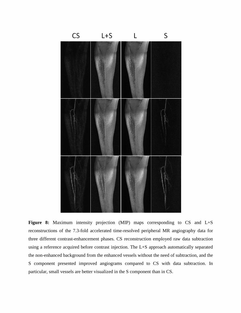
Figure 8: Maximum intensity projection (MIP) maps corresponding to CS and L+S
reconstructions of the 7.3-fold accelerated time-resolved peripheral MR angiography data for
three different contrast-enhancement phases. CS reconstruction employed raw data subtraction
using a reference acquired before contrast injection. The L+S approach automatically separated
the non-enhanced background from the enhanced vessels without the need of subtraction, and the
S component presented improved angiograms compared to CS with data subtraction. In
particular, small vessels are better visualized in the S component than in CS.

Figure 9: CS and L+S reconstruction of 4D dynamic contrast-enhanced abdominal data acquired
with golden-angle radial sampling (8 spokes / frame, undersampling factor = 48, temporal
resolution = 0.94 seconds per 3D volume) corresponding to a representative slice and three
contrast-enhancement phases (aorta, portal vein, liver). L+S compares favorably to CS, and the S
component (right column), in which the background has been suppressed, offers improved
visualization of contrast-enhancement.
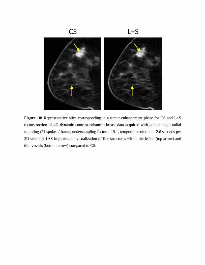
Figure 10: Representative slice corresponding to a tumor-enhancement phase for CS and L+S
reconstruction of 4D dynamic contrast-enhanced breast data acquired with golden-angle radial
sampling (21 spokes / frame, undersampling factor = 19.1, temporal resolution = 2.6 seconds per
3D volume). L+S improves the visualization of fine structures within the lesion (top arrow) and
thin vessels (bottom arrow) compared to CS.
Top Related