Download - LINEAR LAW FOR THE LOGARITHMS OF THE RIEMANN PERIODS … · 2018-11-16 · MATHEMATICS OF COMPUTATION Volume 75, Number 254, Pages 891–902 S 0025-5718(05)01803-X Article electronically

MATHEMATICS OF COMPUTATIONVolume 75, Number 254, Pages 891–902S 0025-5718(05)01803-XArticle electronically published on November 30, 2005

LINEAR LAW FOR THE LOGARITHMSOF THE RIEMANN PERIODS

AT SIMPLE CRITICAL ZETA ZEROS

KEVIN A. BROUGHAN AND A. ROSS BARNETT

Abstract. Each simple zero 12

+ iγn of the Riemann zeta function on the

critical line with γn > 0 is a center for the flow s = ξ(s) of the Riemann xifunction with an associated period Tn. It is shown that, as γn → ∞,

log Tn ≥ π

4γn + O(log γn).

Numerical evaluation leads to the conjecture that this inequality can be re-placed by an equality. Assuming the Riemann Hypothesis and a zeta zeroseparation conjecture γn+1 − γn � γ−θ

n for some exponent θ > 0, we obtainthe upper bound log Tn � γ2+θ

n . Assuming a weakened form of a conjecture

of Gonek, giving a bound for the reciprocal of the derivative of zeta at eachzero, we obtain the expected upper bound for the periods so, conditionally,log Tn = π

4γn + O(log γn). Indeed, this linear relationship is equivalent to the

given weakened conjecture, which implies the zero separation conjecture, pro-vided the exponent is sufficiently large. The frequencies corresponding to theperiods relate to natural eigenvalues for the Hilbert–Polya conjecture. Theymay provide a goal for those seeking a self-adjoint operator related to theRiemann hypothesis.

1. Introduction

If a holomorphic function of a single complex variable f(s) has a simple zeroat so which is a center for the dynamical system s = f(s), then the period of anorbit encircling so is given by 2πi/f ′(so) [3, Theorem 2.3], and, in particular, isindependent of the orbit. When this is applied to the simple zeros of Riemann’sfunction ξ(s), which lie on the critical line s = 1

2 and which coincide with the simplecritical zeros of ζ(s), we see that the periods {τn = 2πi/ξ′( 1

2 +iγn) : ξ( 12 +iγn) = 0}

could be of interest since each such (real) number applies to an infinite family ofnested orbits. See Figure 1 where selected periodic orbits surrounding the 27th and28th zeros of zeta for the flow s = ξ(s) are displayed.

Even though the positions of the zeros on the critical line have a considerabledegree of random variation, the values of the periods are quite constrained, as isillustrated numerically in Figure 2 and partly proved in Theorem 4.1: The logarithmof the absolute value of the periods varies linearly with the position of the zero.

Received by the editor December 13, 2004 and, in revised form, March 17, 2005.2000 Mathematics Subject Classification. Primary 11M06, 11M26, 11S40.Key words and phrases. Riemann zeta function, xi function, zeta zeros, periods, critical line,

Hilbert–Polya conjecture.

c©2005 American Mathematical Society

891

License or copyright restrictions may apply to redistribution; see https://www.ams.org/journal-terms-of-use

892 K. A. BROUGHAN AND A. R. BARNETT

−0.5 0 0.5 1 1.5 2

94.5

95

95.5

96

96.5

97

Figure 1. Orbits around the 27th and 28th zero for z = ξ(z).

In Section 2 the numerical evaluation is developed. Of the 500 zeta zeros studied,being those with smallest positive t coordinates, the periods always increased withincreasing zero value, with four exceptions. The numerical evidence demonstratesa relationship between each period and the t-coordinate of the corresponding zerowhich is very close to being linear.

In Section 3 some preliminary lemmas are given.In Section 4 the relationship

log Tn ≥ π

4γn + O(log γn),

where Tn = (−1)nτn is the absolute value of the period, is proved. An upper boundis derived subject to the Riemann Hypothesis and a plausible conjecture on zeroseparations. Using a weakened form of a conjecture of Gonek (which includes theRiemann Hypothesis), namely, that there exists a nonnegative real number θ suchthat |ζ ′( 1

2 + iγn)|−1 = O(|γn|θ) for all n ∈ N, we derive the precise upper boundand hence, conditionally,

log Tn =π

4γn + O(log γn).

In Section 5 a possible significance of the periods, in the context of the Hilbert–Polya conjecture, is sketched.

We first define some notations. Let s = σ + it, ξ(s) = u(σ, t) + iv(σ, t). Labelthe simple zeros of ξ(s), with a positive t coordinate, going up the critical line as{γn : n ∈ N}. A particular zero 1

2 + iγn has the corresponding period

τn =2πi

ξ′( 12 + iγn)

.


XI PERIODS 893

Because ξ(s) is real on the critical line, vt( 12 , t) = 0, so ξ′( 1

2 + it) = −iut( 12 , t).

Therefore Tn = 2π/|ut( 12 , γn)|.

Let s = 12 + it and write the ξ definition from Section 2 as

ξ( 12 + it) = elog Γ( s

2 )π−s/2 s(s − 1)2

ζ(s)

= −e� log Γ( s2 )π−1/4(

t2 + 1/42

) × Z(t)

= Y (t) × Z(t),

where

log Γ(s + 1) = (s + 12 ) log s − s + c1 + O( 1

s )

Z(t) = eiϑ(t)ζ( 12 + it)

ϑ(t) =t

2log(

t

2π) − t

2− π

8+ O(

1t),

and where here and in what follows the c1, c2, . . . are absolute constants.

2. Numerical evaluation of the periods

We used the Chebyshev method of P. Borwein [2] to evaluate ζ(s). Our versionis described in [3, section 5] in which accuracies for the ζ-zeros γ1 − γ502 betterthan 10−10 were demonstrated.

A program was written in MATLAB using the methods of Godfrey [10] forboth the ζ-function and the complex Γ-function. They are available in Godfrey’sMATLAB site as part of the zeta-function code. In particular, values of the gamma

0 100 200 300 400 500 600 700 800 900−100

0

100

200

300

400

500

600

700

Slope = π / 4

Riemann zero γn of ξ

log

Tn

Figure 2. Plot of logarithm of the period magnitudes against theRiemann zeros up to γ502 = 814.1 · · · .



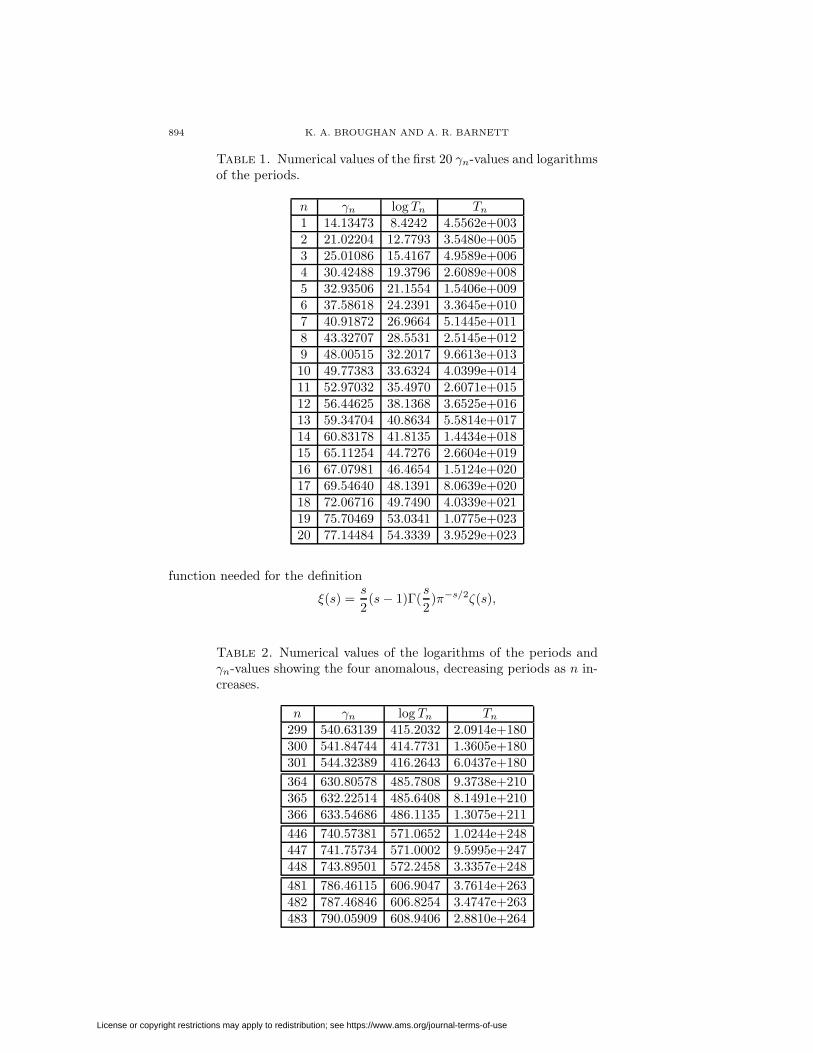
Table 1. Numerical values of the first 20 γn-values and logarithmsof the periods.

n γn log Tn Tn

1 14.13473 8.4242 4.5562e+0032 21.02204 12.7793 3.5480e+0053 25.01086 15.4167 4.9589e+0064 30.42488 19.3796 2.6089e+0085 32.93506 21.1554 1.5406e+0096 37.58618 24.2391 3.3645e+0107 40.91872 26.9664 5.1445e+0118 43.32707 28.5531 2.5145e+0129 48.00515 32.2017 9.6613e+01310 49.77383 33.6324 4.0399e+01411 52.97032 35.4970 2.6071e+01512 56.44625 38.1368 3.6525e+01613 59.34704 40.8634 5.5814e+01714 60.83178 41.8135 1.4434e+01815 65.11254 44.7276 2.6604e+01916 67.07981 46.4654 1.5124e+02017 69.54640 48.1391 8.0639e+02018 72.06716 49.7490 4.0339e+02119 75.70469 53.0341 1.0775e+02320 77.14484 54.3339 3.9529e+023

function needed for the definition

ξ(s) =s

2(s − 1)Γ(

s

2)π−s/2ζ(s),

Table 2. Numerical values of the logarithms of the periods andγn-values showing the four anomalous, decreasing periods as n in-creases.

n γn log Tn Tn

299 540.63139 415.2032 2.0914e+180300 541.84744 414.7731 1.3605e+180301 544.32389 416.2643 6.0437e+180364 630.80578 485.7808 9.3738e+210365 632.22514 485.6408 8.1491e+210366 633.54686 486.1135 1.3075e+211446 740.57381 571.0652 1.0244e+248447 741.75734 571.0002 9.5995e+247448 743.89501 572.2458 3.3357e+248481 786.46115 606.9047 3.7614e+263482 787.46846 606.8254 3.4747e+263483 790.05909 608.9406 2.8810e+264


XI PERIODS 895

0 100 200 300 400 500 600 700 800 900−1

0

1

2

3

4

5

6

Riemann zero γn of the ξ function

log(

Tn)

−

π/4

γ n + 1

0

Figure 3. The residuals using a slope of π/4.

do not have to be incorporated into a Riemann–Siegel formulation. The valuesξ′( 1

2 + iγn) were found by differencing. Figure 2 gives an illustration of the linearrelation of this paper for zeros up to t = γ502 = 814.1 · · · .

530 540 550405

410

415

420

log

T n

625 630 635 640 645480

485

490

495

730 740 750

565

570

575


log

T n

775 780 785 790 795

600

605

610


Figure 4. The first four anomalous deviations from monotonicity (circled).



2 2.2 2.4 2.6 2.8 3 3.2 3.4x 10

4

−4

−2

0

2

4

6


log(

Tn)

−π/

4 γn

+ 3

0

2 2.2 2.4 2.6 2.8 3 3.2 3.4x 104

1.5

2

2.5

3 x 104


log(

Tn)

Figure 5. The linear periods (below) and residuals (above) usinga slope of π/4.

Figure 3 shows the deviations from the linear law log Tn = α + π4 γn. There is a

rise, matching an exponential, at low γ-values. The value of α for the fit is −10.0.Table 1 shows the zeros and periods for 0 < n ≤ 20, where the slope deviates

slightly from π/4, as is seen in Figure 3. The rms deviation for the complete fit is1.5.

Table 2 includes the zeros and periods for γ300 = 541.847 · · · , γ365 = 632.225 · · · ,γ447 = 741.757 · · · , and γ482 = 787.468 · · · , where, anomalously, we find log Tn <log Tn−1 which are the only examples below γ502 where the period decreases. Theseare plotted with an expanded scale in Figure 4. An alternative calculation wasdevised to extend the modest upper value of t ∼ 800 to t ∼ 34000. The same linearrelationship was found to hold. The symbolic ζ-calculations of MapleTM werecombined with Godfrey’s implementation of Lanczos’ Γ-function method. Earliervalues t ≤ 814.1 · · · were confirmed. The results are presented in increments of 500in Figure 5.

3. Preliminary lemmas

Lemma 3.1. As t → ∞

� log Γ(12 + it

2) = −1

8log(9 + 4t2) − π

4t + c2 + O(

1t).

Proof. This follows directly from Stirling’s approximation given in Section 1 above.�

Lemma 3.2. As t → ∞, |ϑ′(t)| = O(log t).

Proof. This follows directly from the expression for ϑ(t) given above or see [8, Page125]. �


XI PERIODS 897

Lemma 3.3. As t → ∞, |ζ( 12 + it)| = O(t1/6 log3/2 t).

Proof. This is [17, Page 99]. �

Lemma 3.4. As t → ∞,

|ζ ′( 12 + it)| = O(t1/4 log2 t)

and |ζ ′′( 12 + it)| = O(t1/4 log4 t).

Proof. These bounds follow from the upper bound for ζ(k)( 12 + it), derived using

the approximate functional equation and Cauchy’s integral formula for the nthderivative given in [13, Page 57], namely,

|ζ(k)( 12 + it)| ≤

∣∣∣ ∑n≤

√t/2π

logk n

n1/2+it

∣∣∣ + logk t∑

1≤j≤k

∣∣∣ ∑n≤

√t/2π

logj n

n1/2−it

∣∣∣

+ O(t−1/4 logk t). �

Lemma 3.5. As t → ∞, Z ′(t) = O(t1/4 log2 t).

Proof. This follows directly from Z(t) = eiϑ(t)ζ( 12 + it) after differentiating and

using Lemmas 3.2 and 3.4. �

4. Lower and upper bounds for the linear relationship

Theorem 4.1. For n ∈ N,

log Tn ≥ π

4γn + O(log γn).

Proof. We first have

|ut( 12 , t)| = |ξ′( 1

2 + it)|

and

iξ′( 12 + it) = Y ′(t)Z(t) + Y (t)Z ′(t).

Since Z(γn) = 0,|ξ′( 1

2 + iγn)| = |Y (γn)| × |Z ′(γn)|.So

log |ut( 12 , γn)| = log |Y (γn)| + log |Z ′(γn)|.

By Lemma 3.1,

log |Y (t)| = � log Γ( 1

2 + it

2

)− 1

4log π + log

(18

+t2

2

)

= −π

4t + log

( 1 + 4t2

(9 + 4t2)1/8

)+ c3 + O

(1t

).

Therefore, by Lemma 3.5,

log |ut( 12 , γn)| ≤ −π

4 γn + O(log γn),

and thereforelog Tn ≥ π

4γn + O(log γn). �



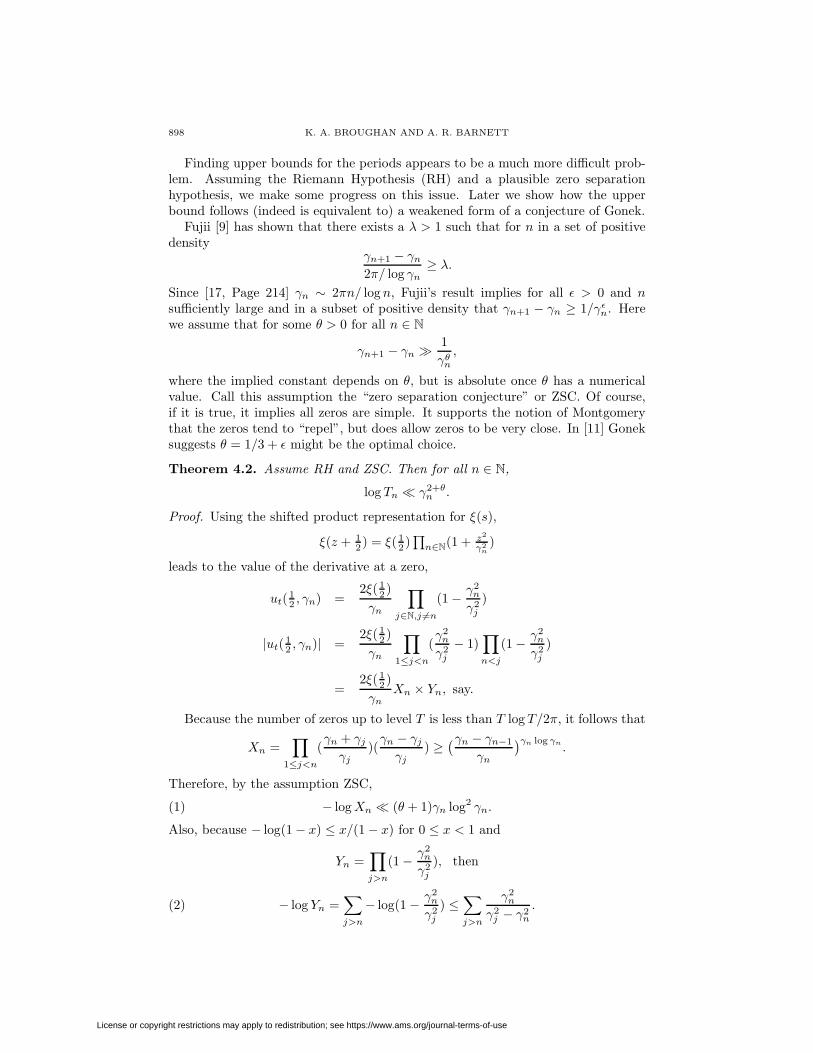
Finding upper bounds for the periods appears to be a much more difficult prob-lem. Assuming the Riemann Hypothesis (RH) and a plausible zero separationhypothesis, we make some progress on this issue. Later we show how the upperbound follows (indeed is equivalent to) a weakened form of a conjecture of Gonek.

Fujii [9] has shown that there exists a λ > 1 such that for n in a set of positivedensity

γn+1 − γn

2π/ log γn≥ λ.

Since [17, Page 214] γn ∼ 2πn/ log n, Fujii’s result implies for all ε > 0 and nsufficiently large and in a subset of positive density that γn+1 − γn ≥ 1/γε

n. Herewe assume that for some θ > 0 for all n ∈ N

γn+1 − γn 1γθ

n

,

where the implied constant depends on θ, but is absolute once θ has a numericalvalue. Call this assumption the “zero separation conjecture” or ZSC. Of course,if it is true, it implies all zeros are simple. It supports the notion of Montgomerythat the zeros tend to “repel”, but does allow zeros to be very close. In [11] Goneksuggests θ = 1/3 + ε might be the optimal choice.

Theorem 4.2. Assume RH and ZSC. Then for all n ∈ N,

log Tn γ2+θn .

Proof. Using the shifted product representation for ξ(s),

ξ(z + 12 ) = ξ( 1

2 )∏

n∈N(1 + z2

γ2n)

leads to the value of the derivative at a zero,

ut( 12 , γn) =

2ξ( 12 )

γn

∏j∈N,j �=n

(1 − γ2n

γ2j

)

|ut( 12 , γn)| =

2ξ( 12 )

γn

∏1≤j<n

(γ2

n

γ2j

− 1)∏n<j

(1 − γ2n

γ2j

)

=2ξ( 1

2 )γn

Xn × Yn, say.

Because the number of zeros up to level T is less than T log T/2π, it follows that

Xn =∏

1≤j<n

(γn + γj

γj)(

γn − γj

γj) ≥

(γn − γn−1

γn

)γn log γn .

Therefore, by the assumption ZSC,

(1) − log Xn (θ + 1)γn log2 γn.

Also, because − log(1 − x) ≤ x/(1 − x) for 0 ≤ x < 1 and

Yn =∏j>n

(1 − γ2n

γ2j

), then

− log Yn =∑j>n

− log(1 − γ2n

γ2j

) ≤∑j>n

γ2n

γ2j − γ2

n

.(2)


XI PERIODS 899

But ∑j>n

1γ2

j − γ2n

=∑

γ2j < 10

9 γ2n

1γ2

j − γ2n

+∑

γ2j ≥ 10

9 γ2n

1γ2

j − γ2n

= S1 + S2, say.

Since, in S2, γj2 − γ2

n ≥ γ2j − 9

10γ2j = 1

10γ2j ,

S2 ≤∑

γ2j ≥ 10

9 γ2n

10γ2

j

log2 γn

γn.

The sum S1 is finite with largest term being the first, which is

1(γn+1 + γn)(γn+1 − γn)

γθn

2γn.

The number of terms is bounded by∫ √

10/9γn

γn

log t dt = O(γnlog γn),

soS1 γθ

n log γn

and therefore by (2)

(3) − log Yn γ2n(γθ

n log γn +log2 γn

γn) γ2+θ

n .

It follows from (1) and (3) that

log Tn − log |ut( 12 , γn)| γ2+θ

n . �Gonek [11] defines

Θ = inf{θ : |ζ ′( 12 + iγn)|−1 = O(|γn|θ) for all n}.

Then [12] the Riemann Hypothesis implies Θ ≥ 0 and the averaged Mertens hy-pothesis ([17, Section 14.29]) implies Θ ≤ 1. Gonek, on the basis of an analogy witheigenvalue statistics for random unitary matrices, conjectures Θ = 1/3. Hughes,Keating and O’Connell [12], following Gonek, surmise that Θ = 1/3 is in line withMontgomery’s pair correlation conjecture [14, 16], which suggests Θ ≥ 1/3. Tosummarise this heuristic argument, the pair correlation conjecture [14] statementis that for fixed a, b with 0 < a ≤ b < ∞, as T → ∞,

|{(γ, γ′) : 0 < γ, γ′ ≤ T, 2πalog T ≤ γ − γ′ ≤ 2πb

log T }|T log T/(2π)

∼∫ b

a

(1 −

( sin πx

πx

)2)dx.

Then a is set to 0 and b small so that the integral may be approximated by π2b3.Even though the conjecture is true for T → ∞, assuming it holds for “small” T

leads to the inequality b T−1/3 so γn+1 − γn γ−1/3n . Finally assuming the

reverse of an argument similar to that used in Theorem 4.3 below holds, we are ledto suppose Θ 1/3.

Here we assume the Riemann Hypothesis and just Θ < ∞, namely, that thereexists a θ ≥ 0 such that

|ζ ′( 12 + iγn)|−1 = O(|γn|θ)

for all n ∈ N. We call this assumption WG or weak Gonek.



Theorem 4.3. Assume the Riemann Hypothesis and WG. Then for all n

log Tn ≤ π

4γn + O(log γn).

Proof. Using Stirling’s approximation to the Gamma function with ρn = 12 + iγn,

log Tn = log 2π − log |ξ′( 12 + iγn)|

= log 2π − log |ρn(ρn − 1)2

| − log |π−ρn/2| − log |Γ(ρn/2)| − log |ζ ′(ρn)|

= − log |Γ(1/4 + iγn/2)| − log |ζ ′(ρn)| + O(log γn)

=π

4γn + log(1/|ζ ′(ρn)|) + O(log γn),

and the result follows. �

The final equation in this proof can then be used to show

Corollary 4.1. Assume the Riemann Hypothesis. Then WG is true if and only if

log Tn ≤ π

4γn + O(log γn).

Theorem 4.4. Assume the Riemann Hypothesis. Then if WG is true there existsθ1 > 0 such that, for all n ∈ N,

γn+1 − γn 1γθ1

n

.

Proof. Expand f(t) = ζ( 12 + it), using Taylor’s theorem about γn as far as γn+1.

There is an η between γn and γn+1 such that

f(γn+1) = f(γn) + if ′(γn)(γn − γn+1) − 12f ′′(η)(γn − γn+1)2,

so γn+1 − γn = 2|f ′(γn)|/|f ′′(η)|.By Lemma 3.4

|ζ ′′( 12 + iη)| η1/4 log4 η ≤ γ

1/4n+1 log4 γn+1 γ

1/4n log4 γn.

Hence

γn+1 − γn 1

γθnγ

1/4n log4 γn

1

γθ+1/4+εn

,

so we can choose θ1 = θ + 1/4 + ε. �

5. Hilbert–Polya conjecture

The well-known approach to proving the Riemann Hypothesis, attributed toPolya and Hilbert [15], is that there is a naturally occurring Hermitian operatorwhose eigenvalues are the zeros of ξ( 1

2 + it), which are therefore real [7, Page 345].There have been many attempts to find such an operator [1], but none so far hasbeen completely successful. The normal interpretation of the heights of the zeros{γn : n ∈ N} is that they correspond to frequencies of some, to be determined,vibrating system.

Consideration of the phase portraits described in [5, 6] in the light of the con-stancy of the period for rotation about each simple zero on the critical line [3,


XI PERIODS 901

Theorem 2.3], gives rise to the notion that an alternative set of potential eigenval-ues might be related to these periods {Tn : n ∈ N} in the usual manner:

fn =1Tn

=λn

2π=

|ut( 12 , γn)|2π

≈ e−πγn

4

2π,

so λi ≈ e−πγi4 . This approach has the following features:

(a) The eigenvalues have a natural relationship to ζ(s).(b) The eigenvalues are the natural frequencies occurring in the flow s = ξ(s).(c) The lowest zero corresponds to the largest eigenvalue and therefore to the

mode of highest energy and largest frequency. This is quite natural, since the valuesof ξ(s) with s real and with values which are large and positive might be regardedas exerting a strong attractive pull on the flow, and would be expected to generatethe greatest energy in the closest pair of zeros, in which corresponding frequenciesbecome the “fundamental” modes. This “attractor” concept is strongly reinforcedby the structure of the separatrices which all tend to the real axis [5, Theorem3.2]. This is much more satisfactory than the normal approach in which the energyincreases as the distance away from the real axis increases.

Acknowledgments

The support of the University of Waikato Department of Mathematics and thehelpful coments of Peter Sarnak and Steve Gonek are warmly acknowledged.

References

[1] Berry, M.V. and Keating, J.P. The Riemann zeros and eigenvalue asympototics. SIAM Re-view 41 (1999), 236-266. MR1684543 (2000f:11107)

[2] Borwein, P. An efficient algorithm for the Riemann zeta function, Constructive, experimentaland nonlinear analysis (Limoges, 1999), CMS Conf. Proc. 27 (2000), 29-34. MR1777614(2001f:11143)

[3] Broughan, K. A. Holomorphic flows on simply connected subsets have no limit cycles. Mec-canica 38 (2003), 699-709. MR2028269 (2004m:37092)

[4] Broughan, K. A. and Barnett, A. R. Holomphic flow of the Riemann zeta function. Math.Comp. 73 (2004), 987-1004. MR2031420 (2004j:11092)

[5] Broughan, K. A. Holomorphic flow of Riemann’s function ξ(s). Nonlinearity 18 (2005), 1269-1294. MR2134894

[6] Broughan, K.A. Phase portraits of the Riemann xi function zeros.http://www.math.waikato.ac.nz/∼kab

[7] Conrey, J.B. The Riemann Hypothesis. Notices AMS 50 (2003), 341-353. MR1954010(2003j:11094)

[8] Edwards, T.M. Riemann’s zeta function. Dover, New York, 1974. MR1854455 (2002g:11129)[9] Fujii, A. On the difference between r consecutive ordinates of the Riemann Zeta function,

Proc. Japan Acad. 51 (1975), 741-743. MR0389781 (52:10612)[10] Godfrey, P. An efficient algorithm for the Riemann zeta function,

http://www.mathworks.com/support/ftp zeta.m, etan.m (2000)[11] Gonek, S.M. The second moment of the reciprocal of the Riemann zeta function and its

derivative, lecture at the Mathematical Sciences Research Institute, Berkeley (June 1999).[12] Hughes, C.P., Keating, J.P. and O’Connell, N. Random matrix theory and the derivative

of the Riemann zeta function, Proceedings of the Royal Society: A 456 (2000), 2611-2627.MR1799857 (2002e:11117)

[13] Levinson, N. and Montgomery, H. L. Zeros of the derivatives of the Riemann zeta function.Acta Math. 133 (1974), 49-65. MR0417074 (54:5135)

[14] Montgomery, H. L. The Pair correlation of zeros of the zeta function. Analytic NumberTheory, Proceedings of the Symposia in Pure Mathematics 24 (1973), 181-193. MR0337821(49:2590)


http://www.ams.org/mathscinet-getitem?mr=1684543






















[15] Odlyzko, A. M. Correspondence about the origins of the Hilbert-Polya conjecture.http://www.dtc.umn.edu/∼oldyzko/polya/

[16] Oldyzko, A. M. On the distribution of spacings between zeros of the zeta function. Math.Comp. 48 (1987), 273-308. MR0866115 (88d:11082)

[17] Titchmarsh, E.C. as revised by Heath-Brown, D.R. The theory of the Riemann Zeta-function.Oxford, Second Ed., 1986. MR0882550 (88c:11049)

Department of Mathematics, University of Waikato, Hamilton, New Zealand

E-mail address: [email protected]

Department of Mathematics, University of Waikato, Hamilton, New Zealand

E-mail address: [email protected]




