


Languages
Pages
Legal

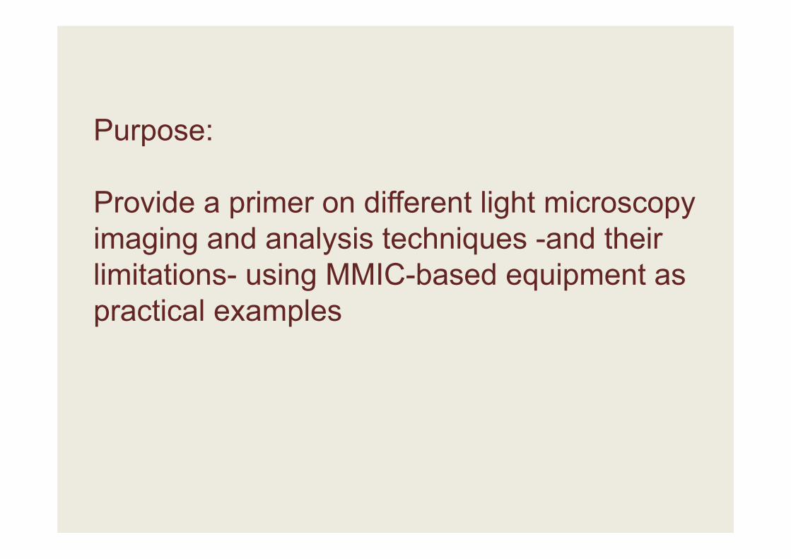
Purpose:
Provide a primer on different light microscopy imaging and analysis techniques -and their limitations- using MMIC-based equipment as practical examples
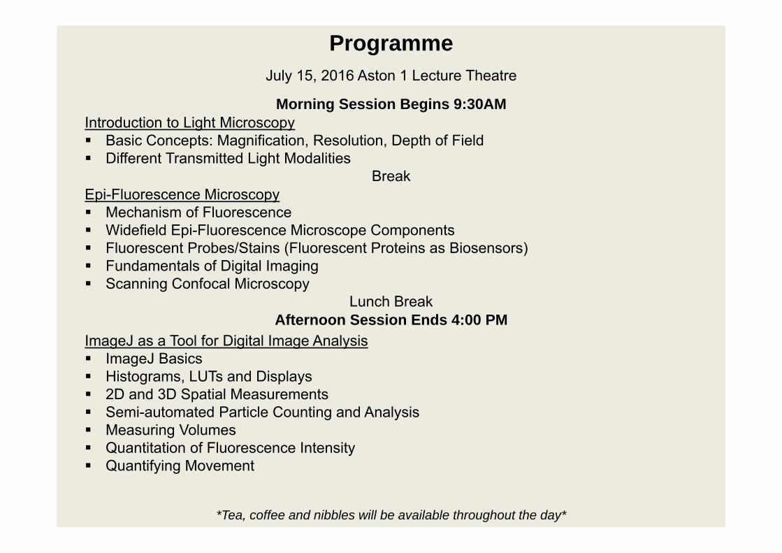
Programme
Introduction to Light Microscopy Basic Concepts: Magnification, Resolution, Depth of Field Different Transmitted Light Modalities
Break
ImageJ as a Tool for Digital Image Analysis ImageJ Basics Histograms, LUTs and Displays 2D and 3D Spatial Measurements Semi-automated Particle Counting and Analysis Measuring Volumes Quantitation of Fluorescence Intensity Quantifying Movement
Morning Session Begins 9:30AM
Afternoon Session Ends 4:00 PM
Epi-Fluorescence Microscopy Mechanism of Fluorescence Widefield Epi-Fluorescence Microscope Components Fluorescent Probes/Stains (Fluorescent Proteins as Biosensors) Fundamentals of Digital Imaging Scanning Confocal Microscopy
Lunch Break
*Tea, coffee and nibbles will be available throughout the day*
July 15, 2016 Aston 1 Lecture Theatre
Principles of MicroscopyMicroscopy allows us to view processes that would not be
visible to the naked eye
Object too small - we cannot see objects smaller than about 0.1mm or the thickness of a human hair)
Object lacks contrast (Stains/Phase-Contrast/DIC)
Process too slow (time-lapse) or not visible in nature (molecular dynamics or interactions-FRAP, FRET)
Every microscope has limits
Poor sample preparation is a recipe for disappointment and poor imaging
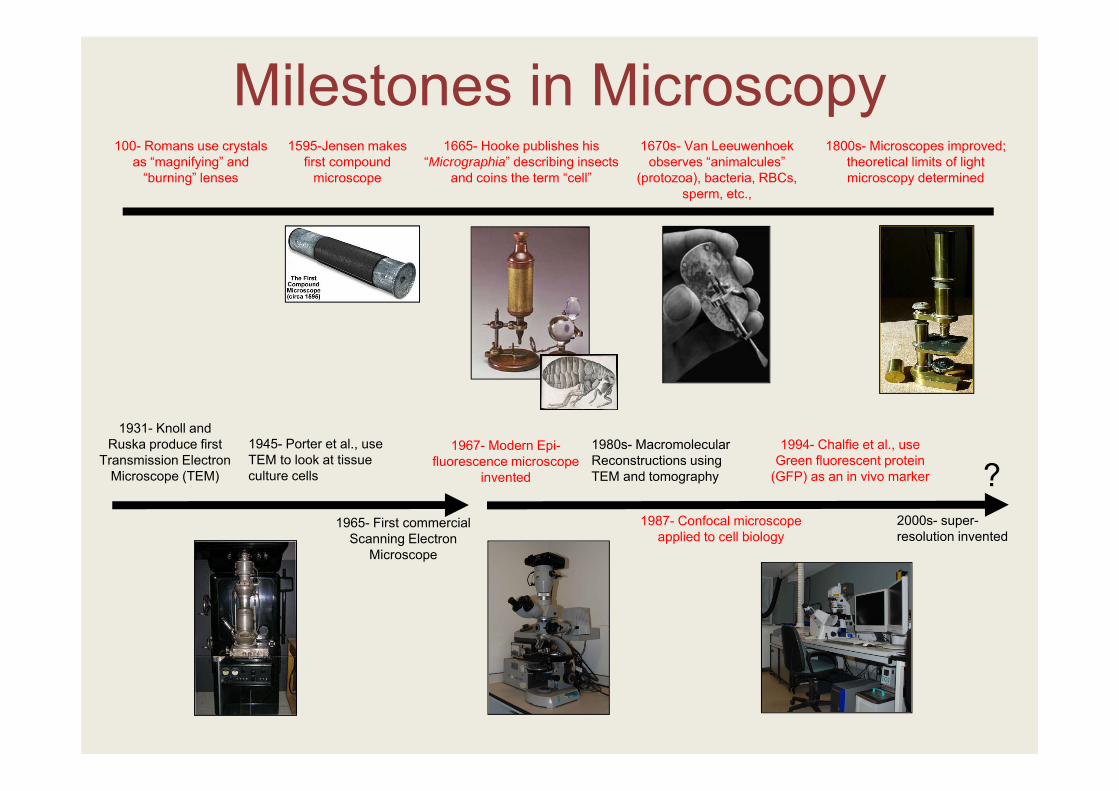
Milestones in Microscopy1595-Jensen makes
first compound microscope
1670s- Van Leeuwenhoek observes “animalcules”
(protozoa), bacteria, RBCs, sperm, etc.,
1967- Modern Epi-fluorescence microscope
invented
1800s- Microscopes improved; theoretical limits of light microscopy determined
1665- Hooke publishes his “Micrographia” describing insects
and coins the term “cell”
100- Romans use crystals as “magnifying” and
“burning” lenses
1994- Chalfie et al., use Green fluorescent protein
(GFP) as an in vivo marker
1931- Knoll and Ruska produce first
Transmission Electron Microscope (TEM)
1945- Porter et al., use TEM to look at tissue culture cells
1965- First commercial Scanning Electron
Microscope
1980s- Macromolecular Reconstructions using TEM and tomography ?
1987- Confocal microscope applied to cell biology
2000s- super-resolution invented
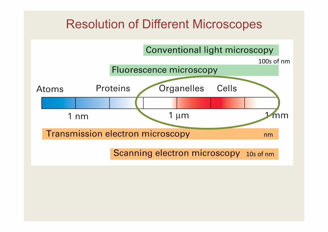
Resolution of Different Microscopes
nm
10s of nm
100s of nm
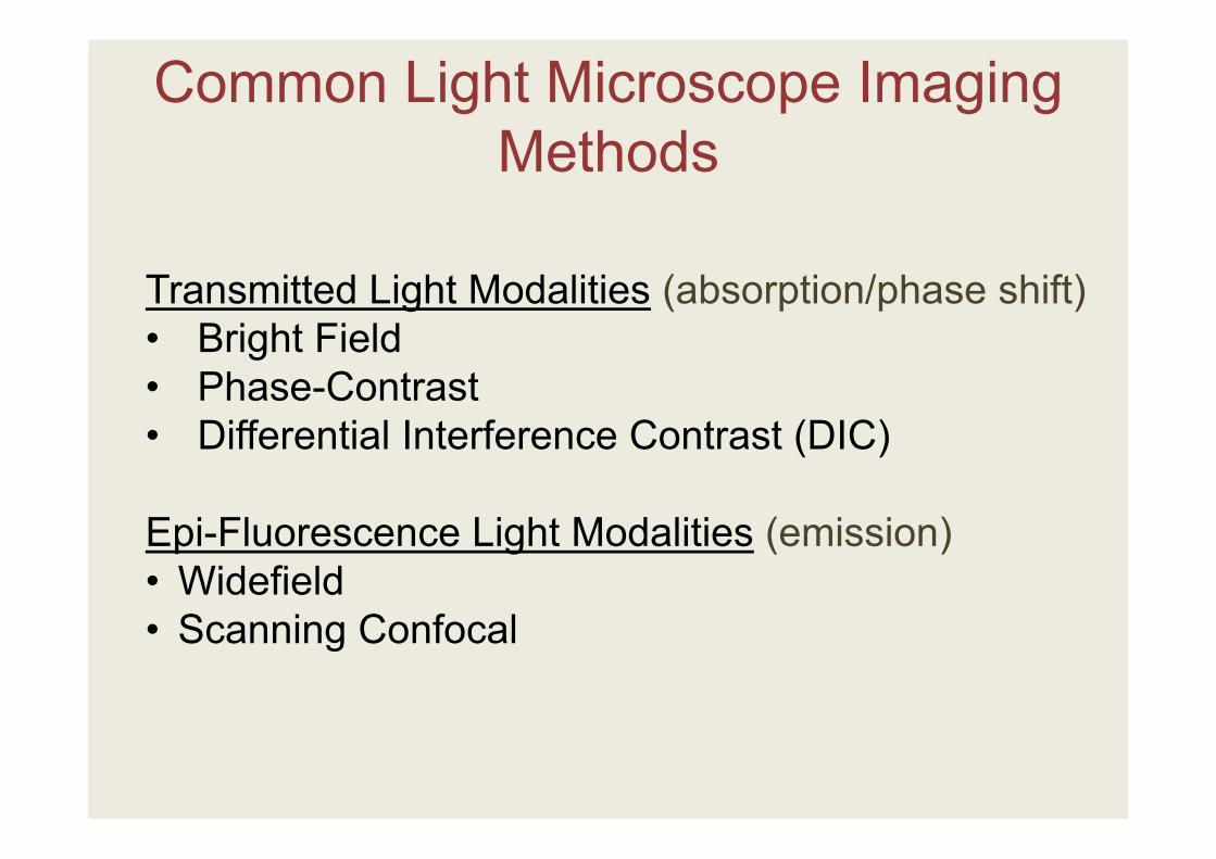
Transmitted Light Modalities (absorption/phase shift)• Bright Field • Phase-Contrast • Differential Interference Contrast (DIC)
Epi-Fluorescence Light Modalities (emission)• Widefield• Scanning Confocal
Common Light Microscope Imaging Methods
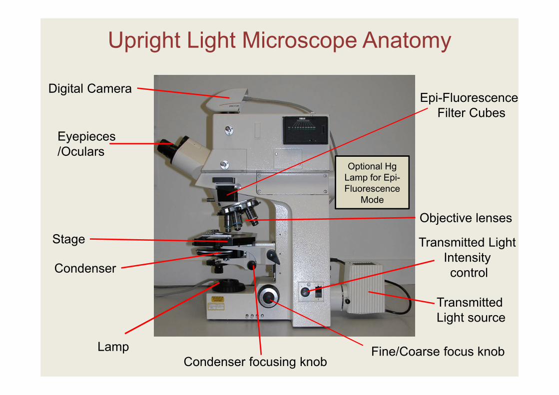
Upright Light Microscope Anatomy
Eyepieces/Oculars
Digital Camera
Stage
Objective lenses
TransmittedLight source
Transmitted Light Intensity control
Fine/Coarse focus knobCondenser focusing knob
Condenser
Lamp
Optional Hg Lamp for Epi-Fluorescence
Mode
Epi-Fluorescence Filter Cubes
IMAGE FORMATION:Attributes of Microscopes
Magnification
Resolution
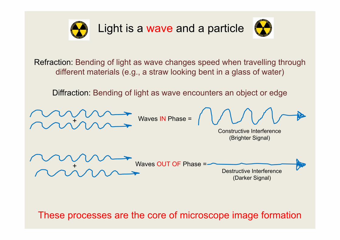
Refraction: Bending of light as wave changes speed when travelling through different materials (e.g., a straw looking bent in a glass of water)
Diffraction: Bending of light as wave encounters an object or edge
These processes are the core of microscope image formation
Waves OUT OF Phase =
Waves IN Phase =+
+
Constructive Interference (Brighter Signal)
Destructive Interference (Darker Signal)
Light is a wave and a particle
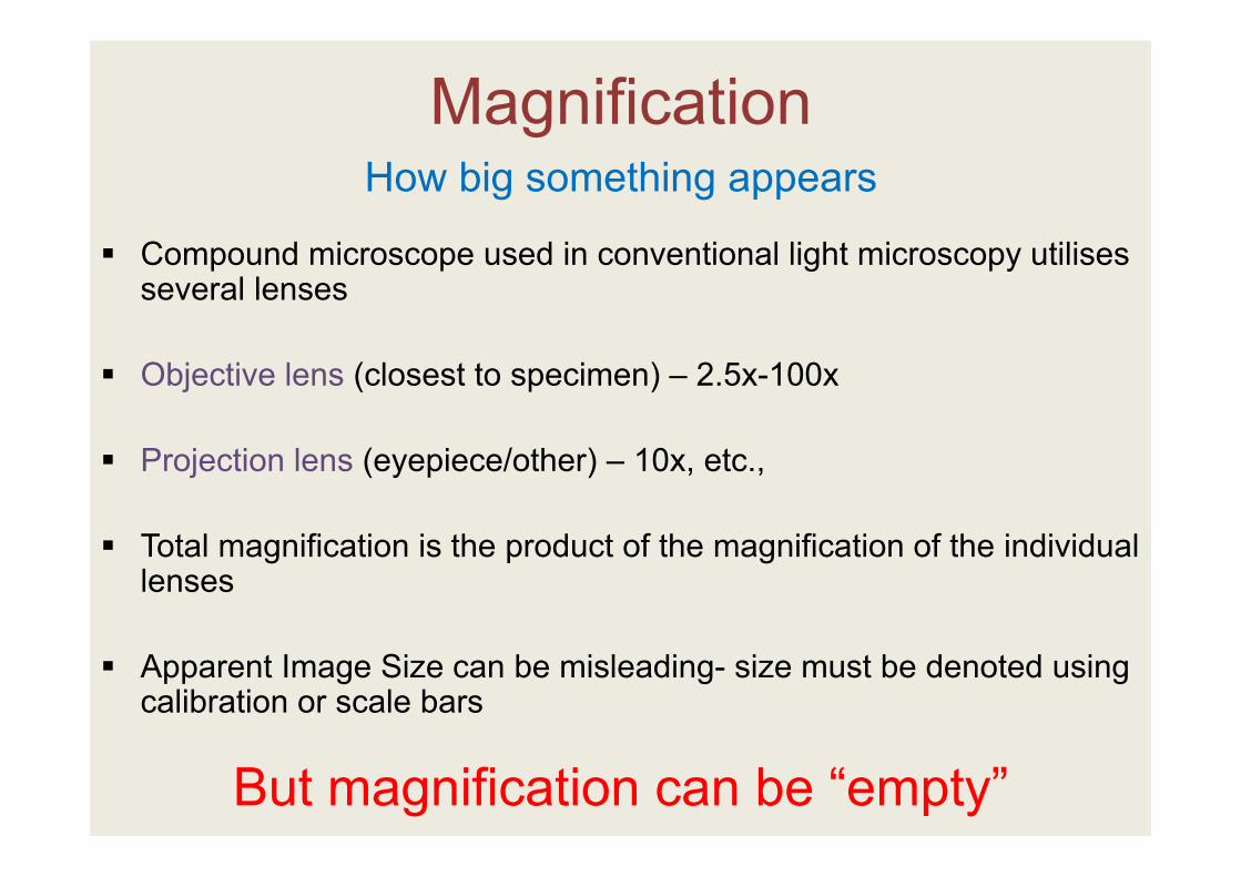
Magnification
Compound microscope used in conventional light microscopy utilisesseveral lenses
Objective lens (closest to specimen) – 2.5x-100x
Projection lens (eyepiece/other) – 10x, etc.,
Total magnification is the product of the magnification of the individual lenses
Apparent Image Size can be misleading- size must be denoted using calibration or scale bars
But magnification can be “empty”
How big something appears
ResolutionWhat is resolution?
Smallest distance apart at which two points on a specimen can still be seen separately
This is directly related to the light collecting capability of the optical system
---The Objective Lens---
The Diffraction Pattern Defines the Image Characteristics
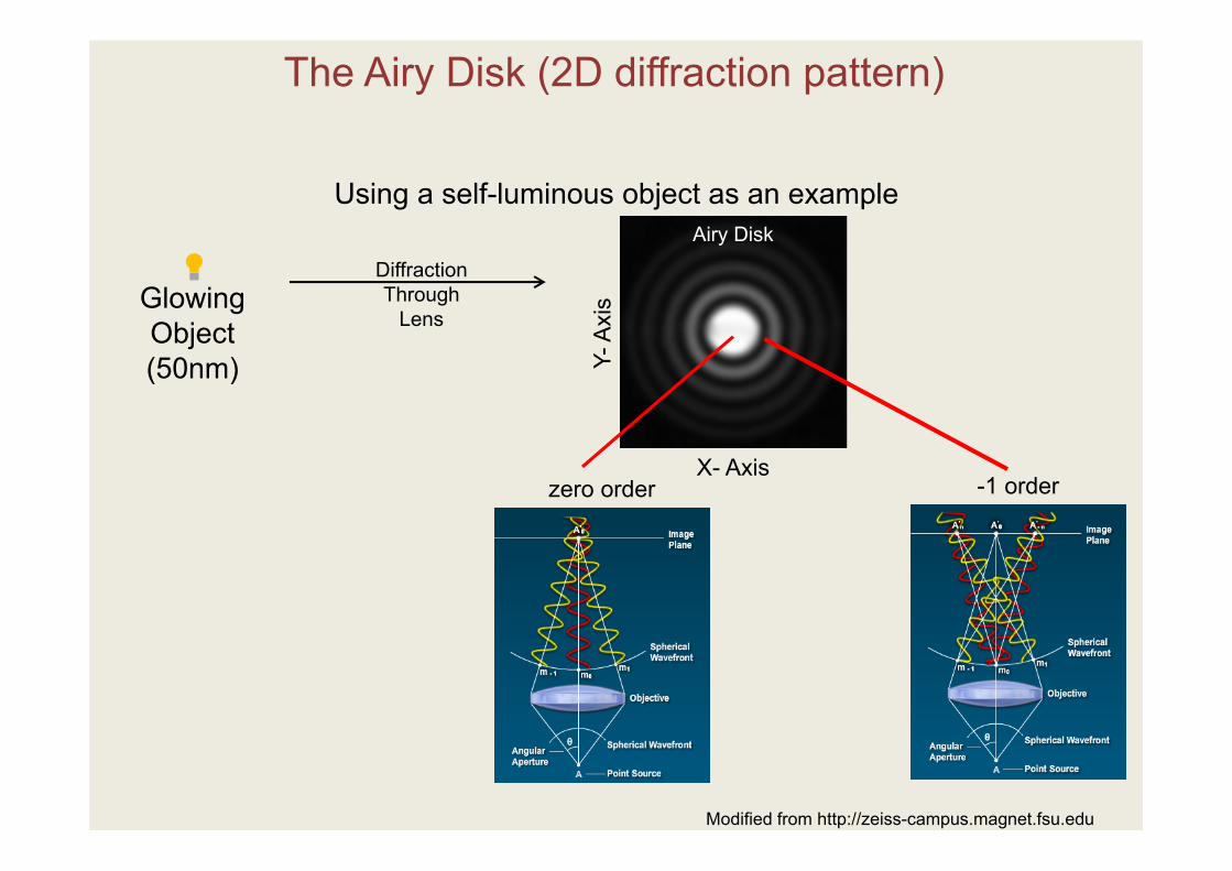
The Airy Disk (2D diffraction pattern)
Using a self-luminous object as an example
Glowing Object(50nm)
DiffractionThrough
Lens
Airy Disk
Y-A
xis
X- Axiszero order -1 order
Modified from http://zeiss-campus.magnet.fsu.edu
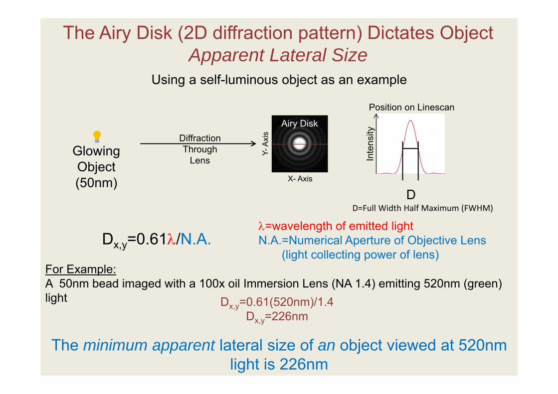
The Airy Disk (2D diffraction pattern) Dictates Object Apparent Lateral Size
For Example:A 50nm bead imaged with a 100x oil Immersion Lens (NA 1.4) emitting 520nm (green) light Dx,y=0.61(520nm)/1.4
Dx,y=226nm
The minimum apparent lateral size of an object viewed at 520nm light is 226nm
Glowing Object(50nm)
DiffractionThrough
Lens Inte
nsity
=wavelength of emitted lightN.A.=Numerical Aperture of Objective Lens
(light collecting power of lens)Dx,y=0.61/N.A.
D=Full Width Half Maximum (FWHM)D
Airy Disk
Y-Ax
is
X- Axis
Position on Linescan
Using a self-luminous object as an example
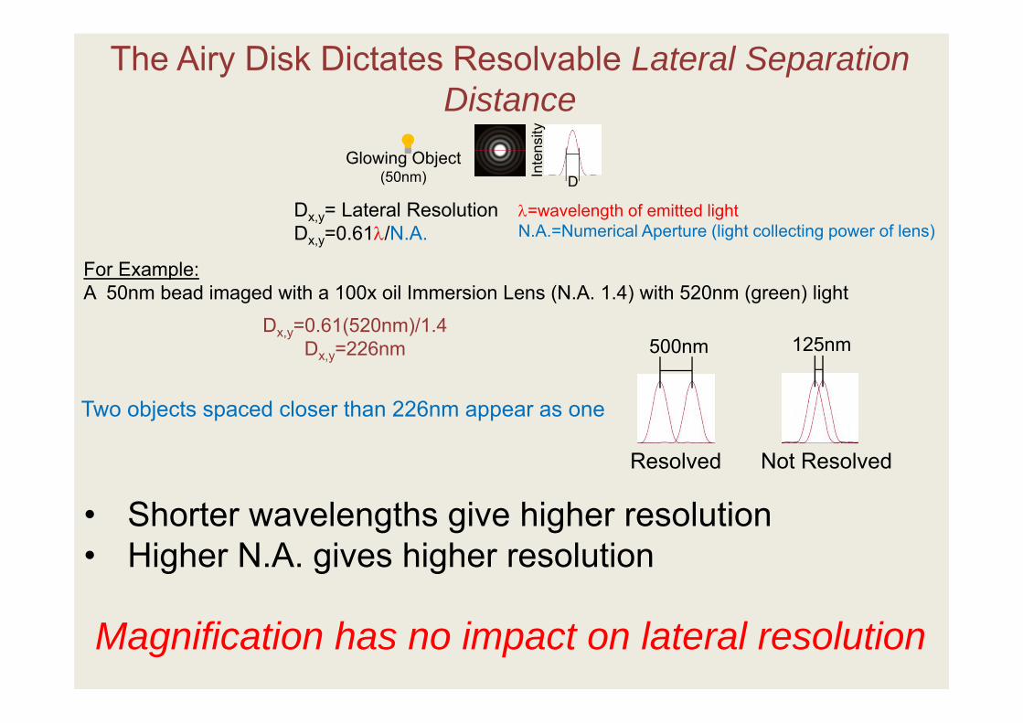
The Airy Disk Dictates Resolvable Lateral SeparationDistance
=wavelength of emitted lightN.A.=Numerical Aperture (light collecting power of lens)
Glowing Object(50nm) In
tens
ity
D
Dx,y= Lateral ResolutionDx,y=0.61/N.A.
For Example:A 50nm bead imaged with a 100x oil Immersion Lens (N.A. 1.4) with 520nm (green) light
500nm
Resolved
125nm
Not Resolved
Two objects spaced closer than 226nm appear as one
• Shorter wavelengths give higher resolution• Higher N.A. gives higher resolution
Dx,y=0.61(520nm)/1.4Dx,y=226nm
Magnification has no impact on lateral resolution
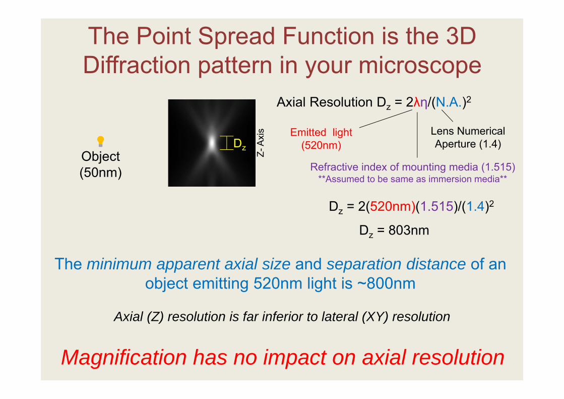
The Point Spread Function is the 3D Diffraction pattern in your microscope
Axial Resolution Dz = 2λη/(N.A.)2
Z-A
xis
Dz
Lens Numerical Aperture (1.4)
Refractive index of mounting media (1.515)**Assumed to be same as immersion media**
Emitted light(520nm)
Dz = 2(520nm)(1.515)/(1.4)2
Dz = 803nm
The minimum apparent axial size and separation distance of an object emitting 520nm light is ~800nm
Axial (Z) resolution is far inferior to lateral (XY) resolution
Magnification has no impact on axial resolution
Object(50nm)
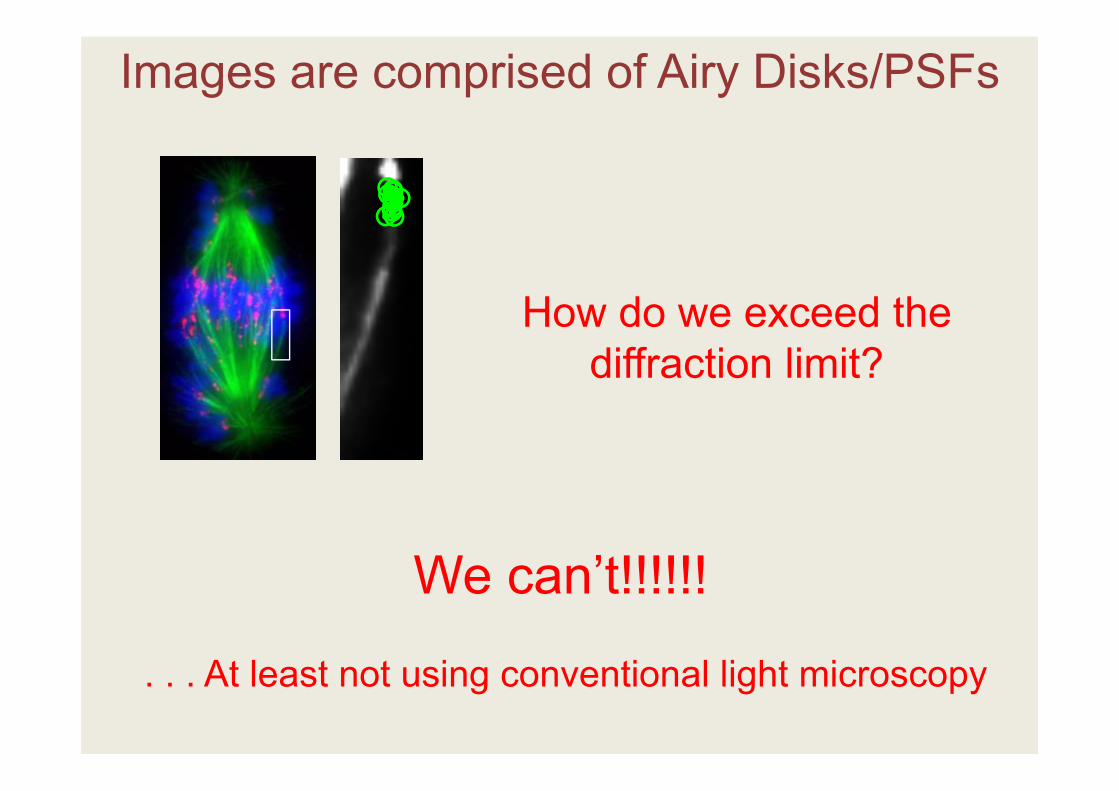
Images are comprised of Airy Disks/PSFs
How do we exceed the diffraction limit?
We can’t!!!!!!
. . . At least not using conventional light microscopy
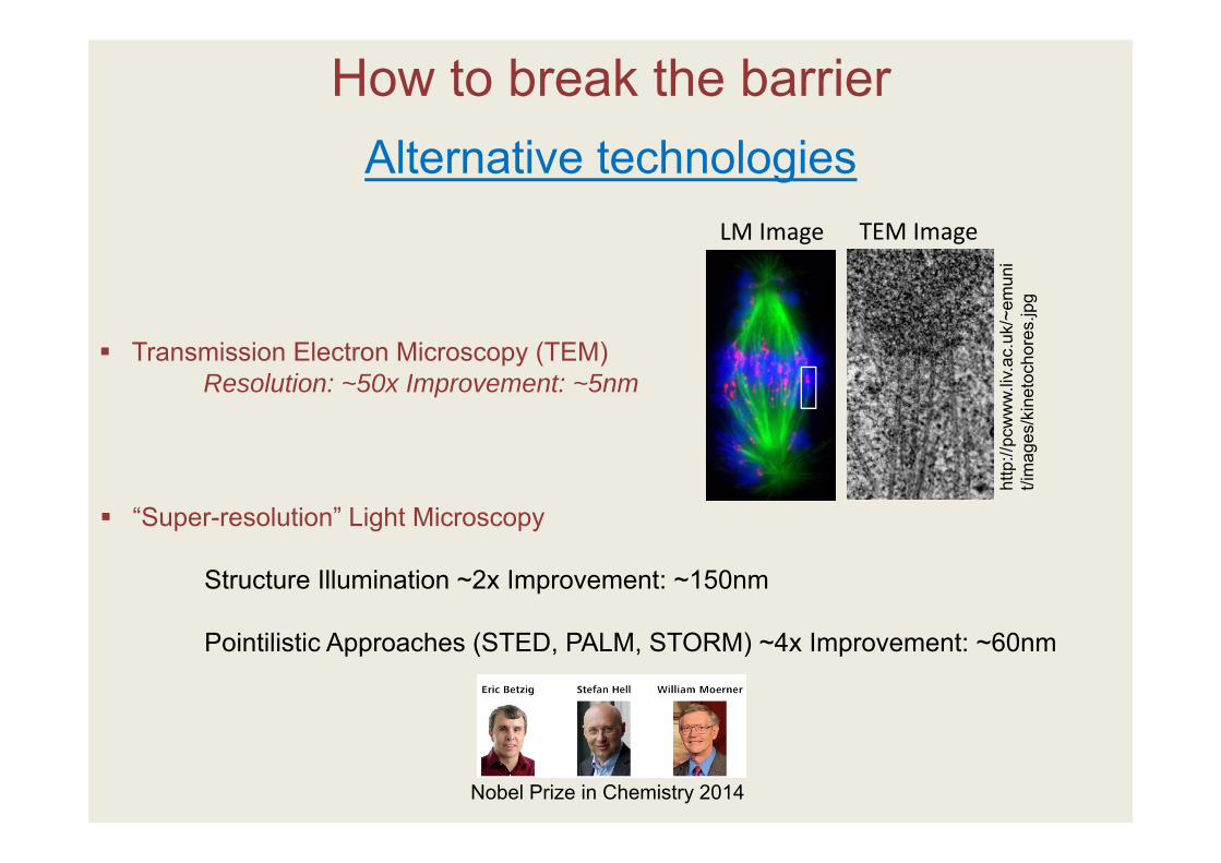
How to break the barrierAlternative technologies
“Super-resolution” Light Microscopy
Structure Illumination ~2x Improvement: ~150nm
Pointilistic Approaches (STED, PALM, STORM) ~4x Improvement: ~60nm
http
://pc
ww
w.liv
.ac.
uk/~
emun
it/i
mag
es/k
inet
ocho
res.
jpg
TEM Image
Transmission Electron Microscopy (TEM)Resolution: ~50x Improvement: ~5nm
LM Image
Nobel Prize in Chemistry 2014
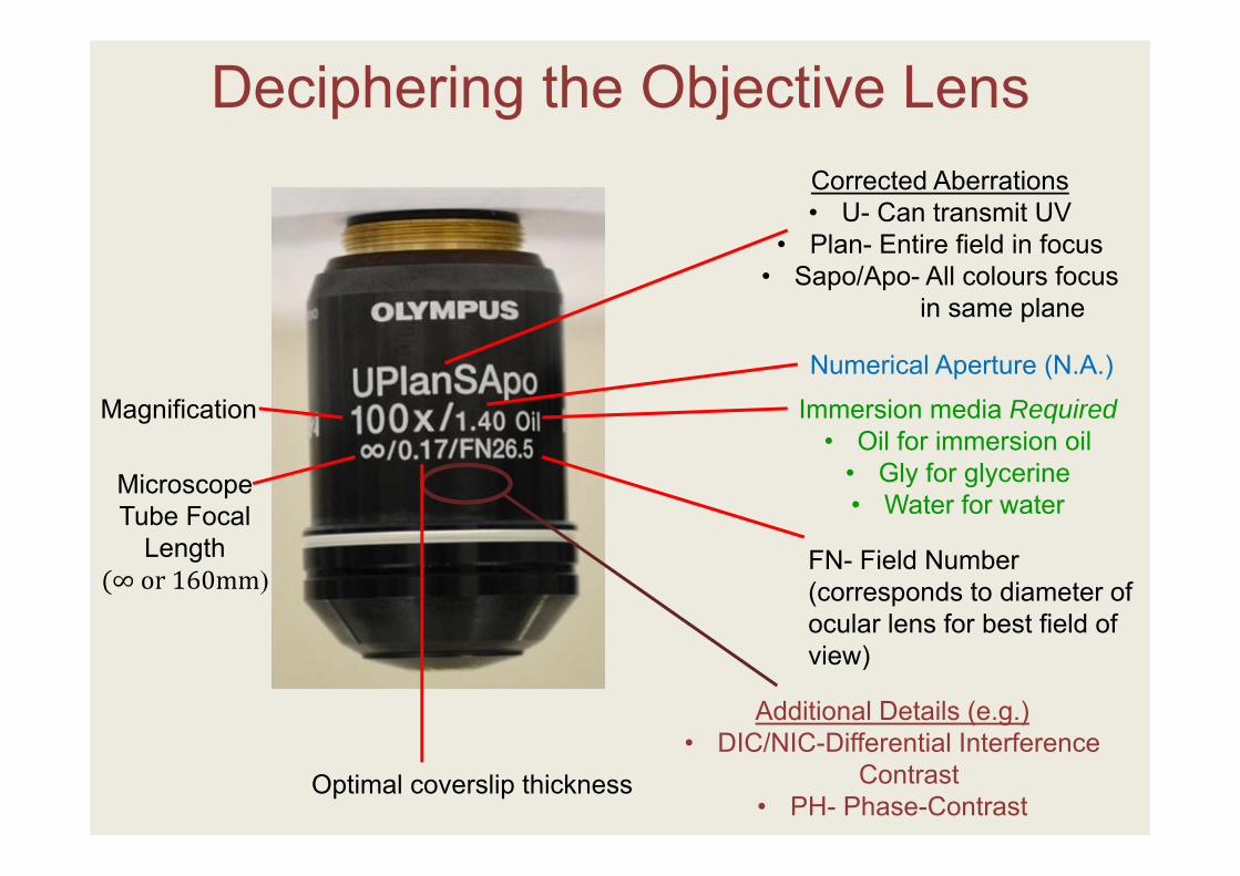
Deciphering the Objective Lens
MicroscopeTube Focal
Length∞or160mm
Immersion media Required• Oil for immersion oil
• Gly for glycerine• Water for water
Optimal coverslip thickness
Corrected Aberrations• U- Can transmit UV
• Plan- Entire field in focus• Sapo/Apo- All colours focus
in same plane
FN- Field Number (corresponds to diameter of ocular lens for best field of view)
Additional Details (e.g.)• DIC/NIC-Differential Interference
Contrast• PH- Phase-Contrast
Magnification
Numerical Aperture (N.A.)
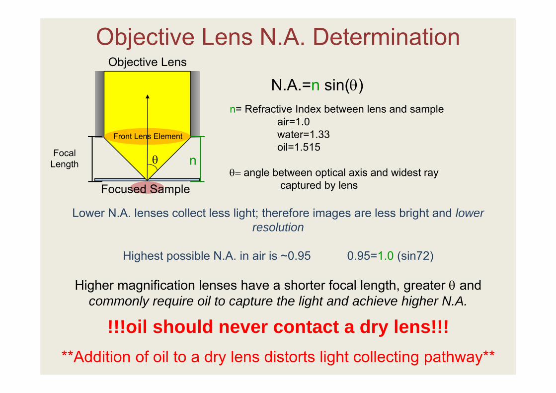
Objective Lens N.A. Determination
Front Lens Element
Objective Lens
N.A.=n sin()n= Refractive Index between lens and sample
air=1.0water=1.33oil=1.515
angle between optical axis and widest raycaptured by lens
Focal Length
Lower N.A. lenses collect less light; therefore images are less bright and lower resolution
Highest possible N.A. in air is ~0.95 0.95=1.0 (sin72)
Higher magnification lenses have a shorter focal length, greater and commonly require oil to capture the light and achieve higher N.A.
n
Focused Sample
!!!oil should never contact a dry lens!!!**Addition of oil to a dry lens distorts light collecting pathway**
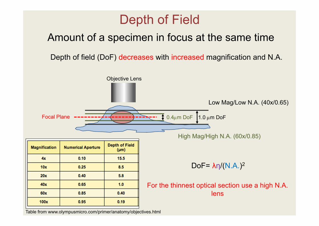
Depth of FieldAmount of a specimen in focus at the same time
Table from www.olympusmicro.com/primer/anatomy/objectives.html
High Mag/High N.A. (60x/0.85)
Focal Plane
Objective Lens
0.4m DoF 1.0 m DoF
Low Mag/Low N.A. (40x/0.65)
Depth of field (DoF) decreases with increased magnification and N.A.
For the thinnest optical section use a high N.A. lens
DoF= λη/(N.A.)2
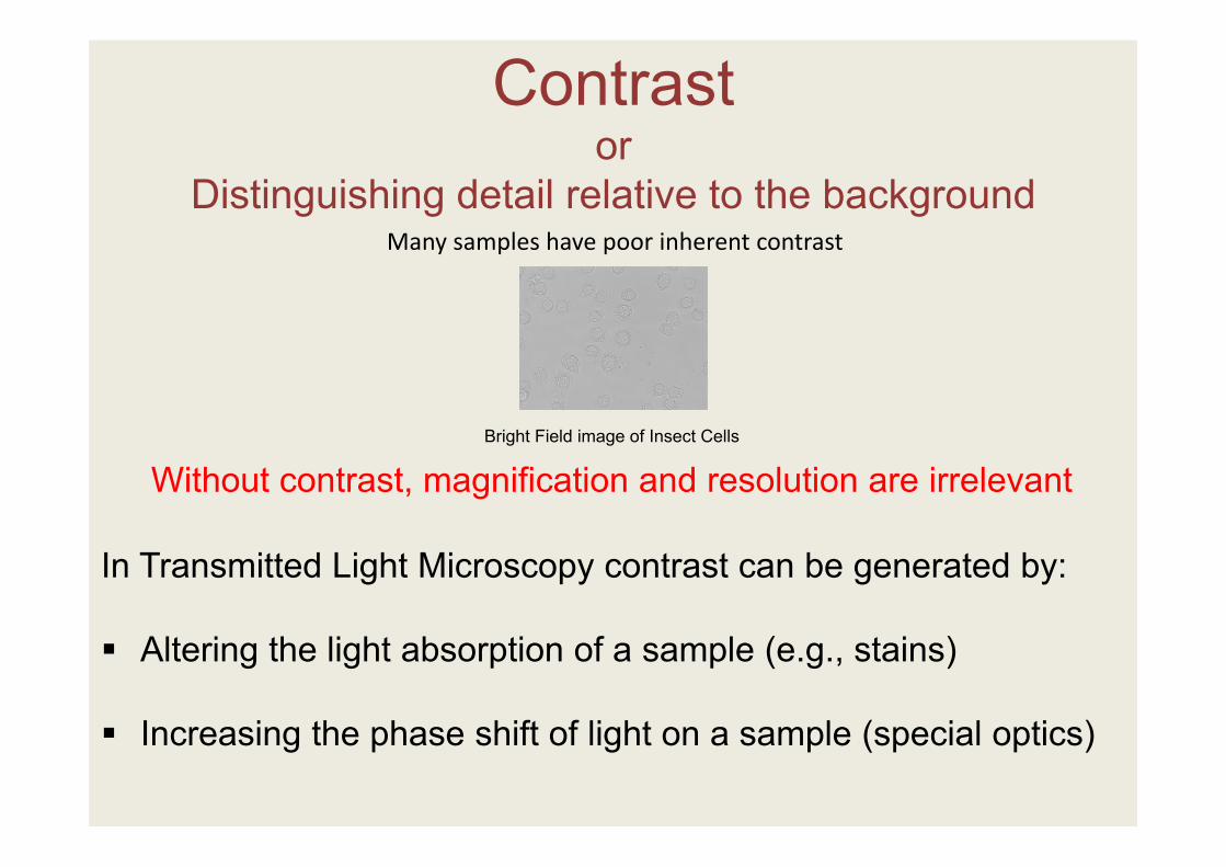
Contrastor
Distinguishing detail relative to the backgroundMany samples have poor inherent contrast
In Transmitted Light Microscopy contrast can be generated by:
Altering the light absorption of a sample (e.g., stains)
Increasing the phase shift of light on a sample (special optics)
Without contrast, magnification and resolution are irrelevantBright Field image of Insect Cells
Transmitted Light Optical Contrasting Techniques
Bright Field
Phase-Contrast
DIC/NIC (Differential Interference Contrast/Nomarski Interference Contrast)
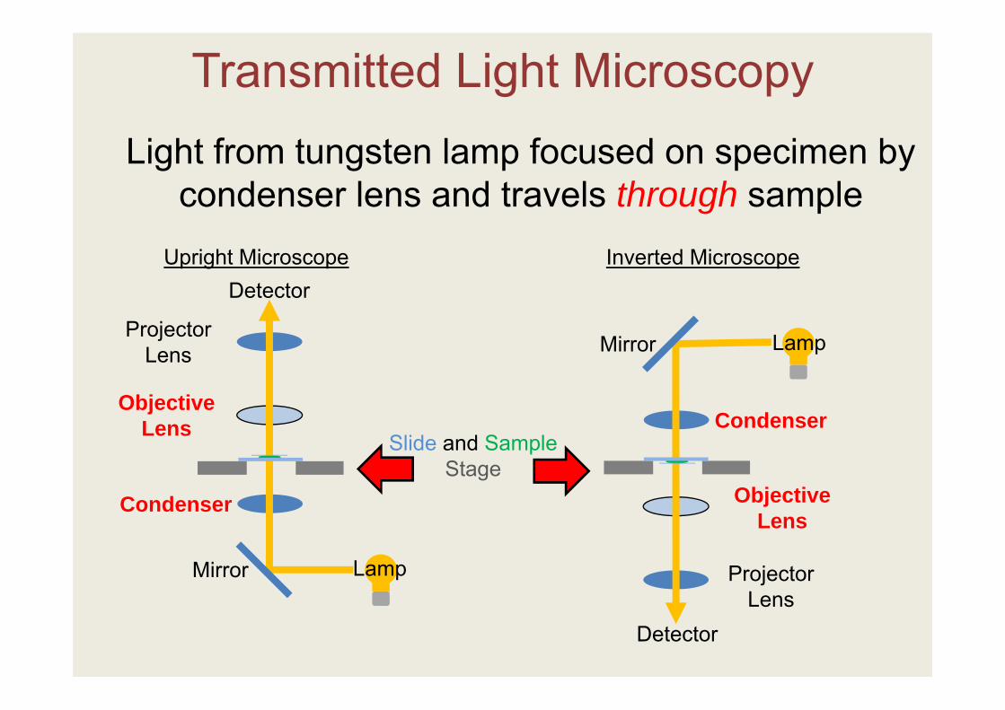
Light from tungsten lamp focused on specimen by condenser lens and travels through sample
Transmitted Light Microscopy
Detector
Slide and SampleStage
Condenser
Objective Lens
Projector Lens
Mirror Lamp
Detector
Projector Lens
Objective Lens
LampMirror
Condenser
Upright Microscope Inverted Microscope
Köehler Illumination
August Köehler, of the Zeiss corporation invented Köehlerillumination in 1893
Samples are uniformly illuminated
Glare and unwanted stray light minimised
Maximise resolution and contrast
To achieve highest quality images it is essential that the sample is correctly illuminated
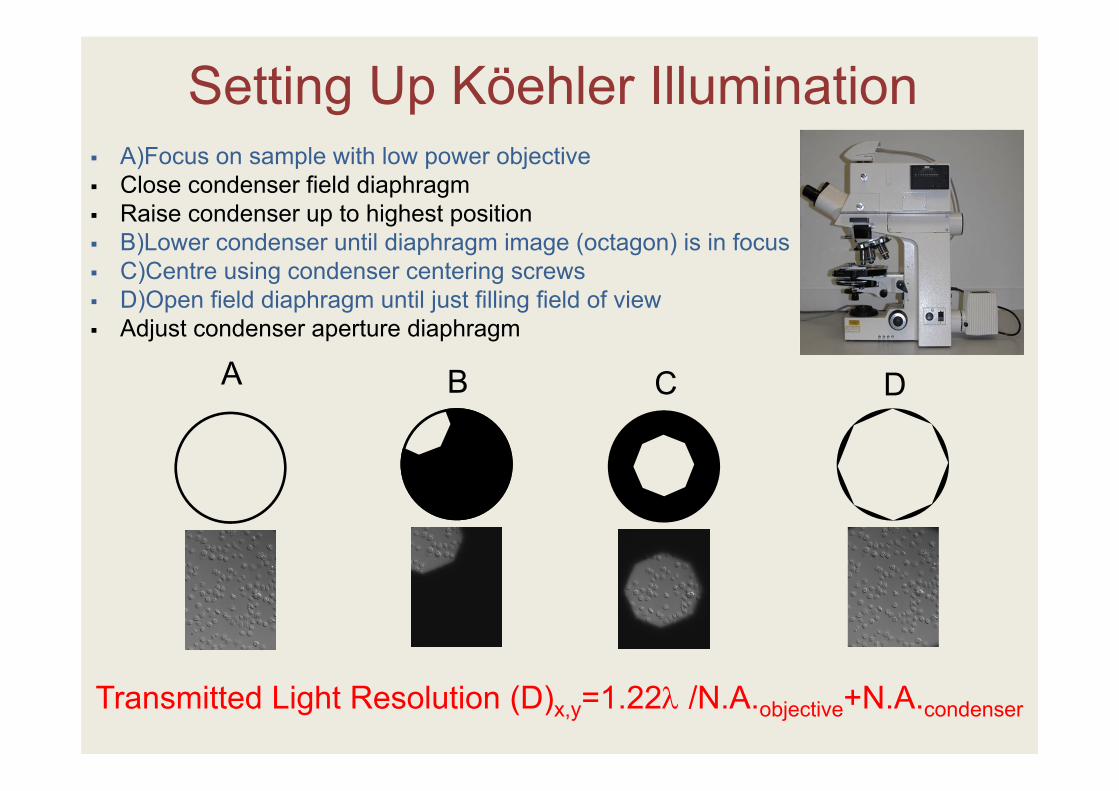
A)Focus on sample with low power objective Close condenser field diaphragm Raise condenser up to highest position B)Lower condenser until diaphragm image (octagon) is in focus C)Centre using condenser centering screws D)Open field diaphragm until just filling field of view Adjust condenser aperture diaphragm
Setting Up Köehler Illumination
B C DA
Transmitted Light Resolution (D)x,y=1.22 /N.A.objective+N.A.condenser
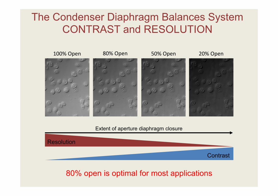
The Condenser Diaphragm Balances System CONTRAST and RESOLUTION
100% Open 80% Open 50% Open 20% Open
Contrast
Resolution
Extent of aperture diaphragm closure
80% open is optimal for most applications
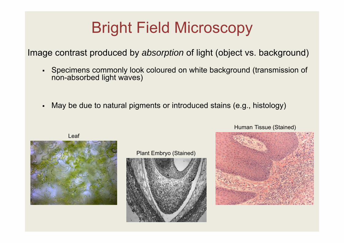
Bright Field MicroscopyImage contrast produced by absorption of light (object vs. background)
Specimens commonly look coloured on white background (transmission of non-absorbed light waves)
May be due to natural pigments or introduced stains (e.g., histology)
Plant Embryo (Stained)
Human Tissue (Stained)Leaf
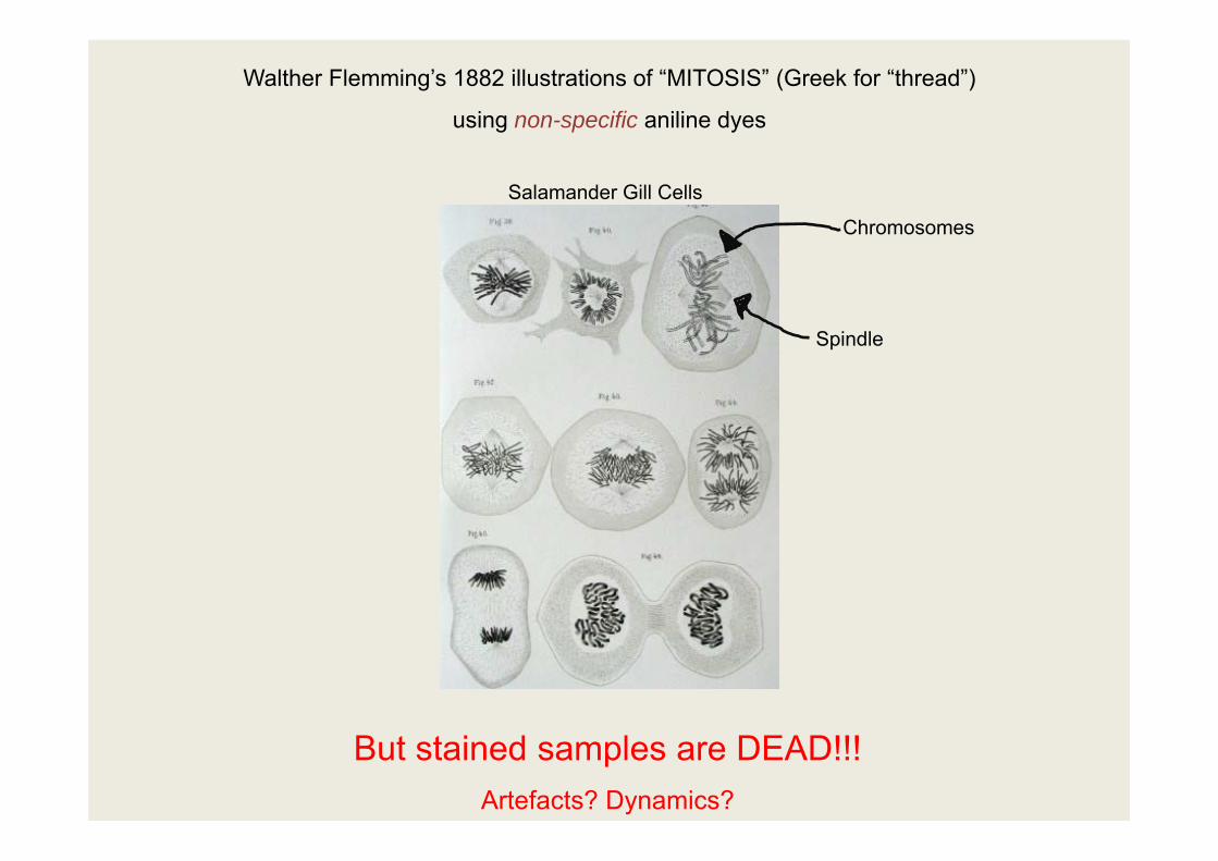
Walther Flemming’s 1882 illustrations of “MITOSIS” (Greek for “thread”)
using non-specific aniline dyes
Salamander Gill Cells
But stained samples are DEAD!!!Artefacts? Dynamics?
Chromosomes
Spindle
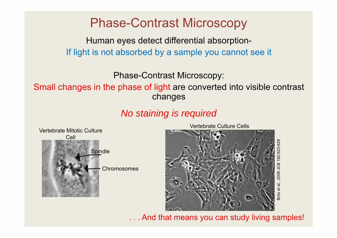
Phase-Contrast MicroscopyHuman eyes detect differential absorption-
If light is not absorbed by a sample you cannot see it
Phase-Contrast Microscopy: Small changes in the phase of light are converted into visible contrast
changes
Vertebrate Mitotic Culture Cell
No staining is required
. . . And that means you can study living samples!
Brit
o et
al.,
200
8 JC
B 1
82:6
23-6
29
Chromosomes
Spindle
Vertebrate Culture Cells
Phase-Contrast Microscopy
www.olympusmicro.com/primer/techniques/phasecontrast/phase.html
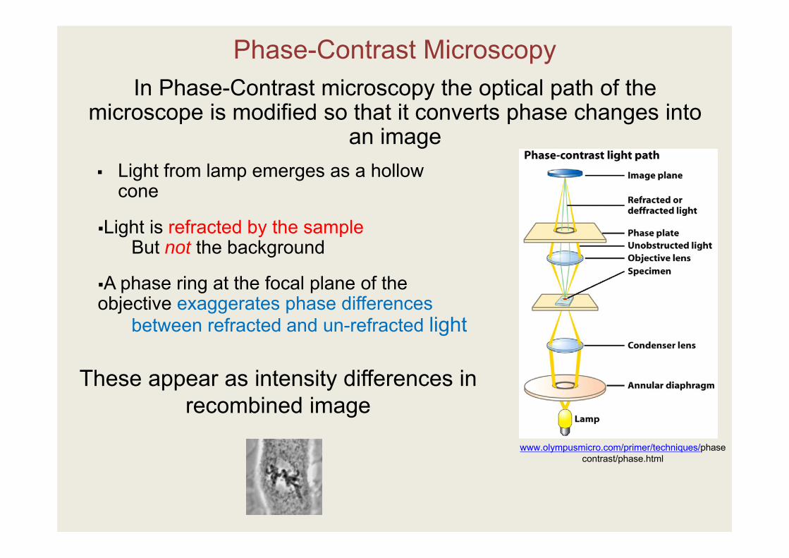
Light from lamp emerges as a hollow cone
In Phase-Contrast microscopy the optical path of the microscope is modified so that it converts phase changes into
an image
These appear as intensity differences in recombined image
A phase ring at the focal plane of the objective exaggerates phase differences
between refracted and un-refracted light
Light is refracted by the sampleBut not the background
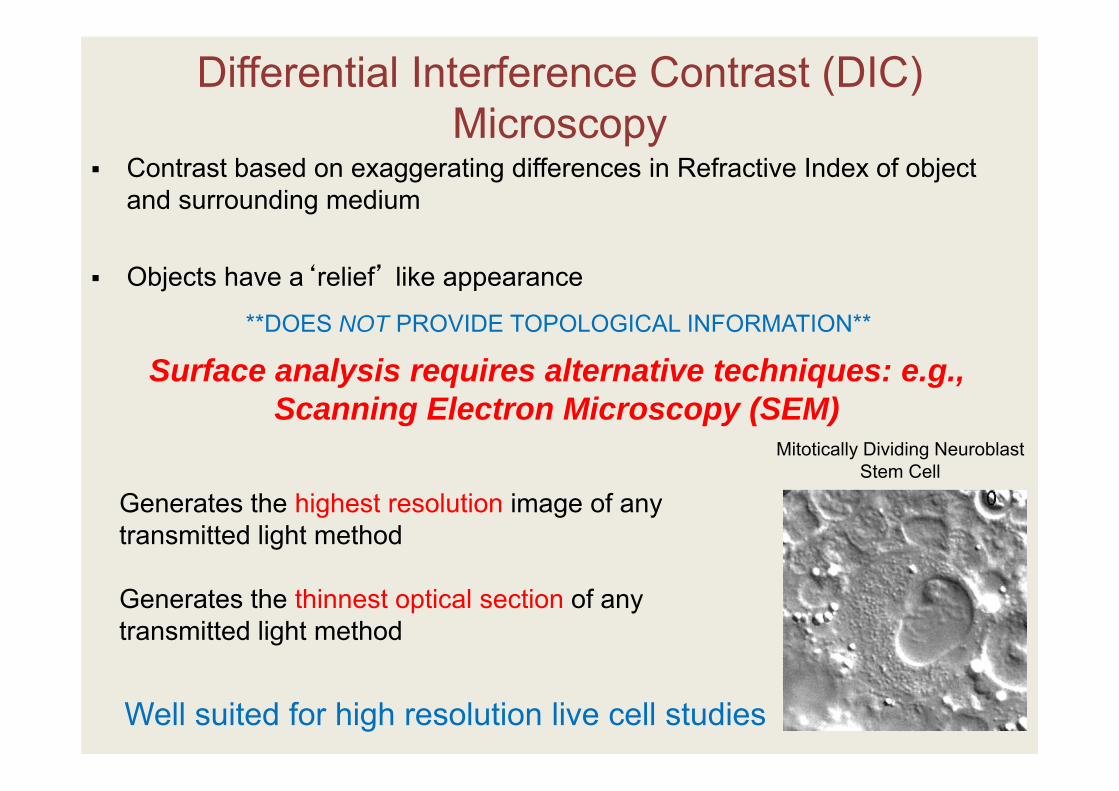
Differential Interference Contrast (DIC) Microscopy
Contrast based on exaggerating differences in Refractive Index of object and surrounding medium
Objects have a‘relief’ like appearance
Surface analysis requires alternative techniques: e.g., Scanning Electron Microscopy (SEM)
**DOES NOT PROVIDE TOPOLOGICAL INFORMATION**
Generates the highest resolution image of any transmitted light method
Generates the thinnest optical section of any transmitted light method
Well suited for high resolution live cell studies
Mitotically Dividing NeuroblastStem Cell
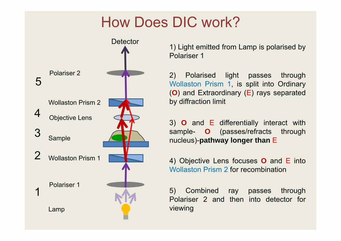
1) Light emitted from Lamp is polarised byPolariser 1
2) Polarised light passes throughWollaston Prism 1, is split into Ordinary(O) and Extraordinary (E) rays separatedby diffraction limit
3) O and E differentially interact withsample- O (passes/refracts throughnucleus)-pathway longer than E
4) Objective Lens focuses O and E intoWollaston Prism 2 for recombination
5) Combined ray passes throughPolariser 2 and then into detector forviewing
1
2
3
4
5
Detector
Wollaston Prism 1
Polariser 1
Polariser 2
Wollaston Prism 2
Objective Lens
Sample
Lamp
How Does DIC work?
PP
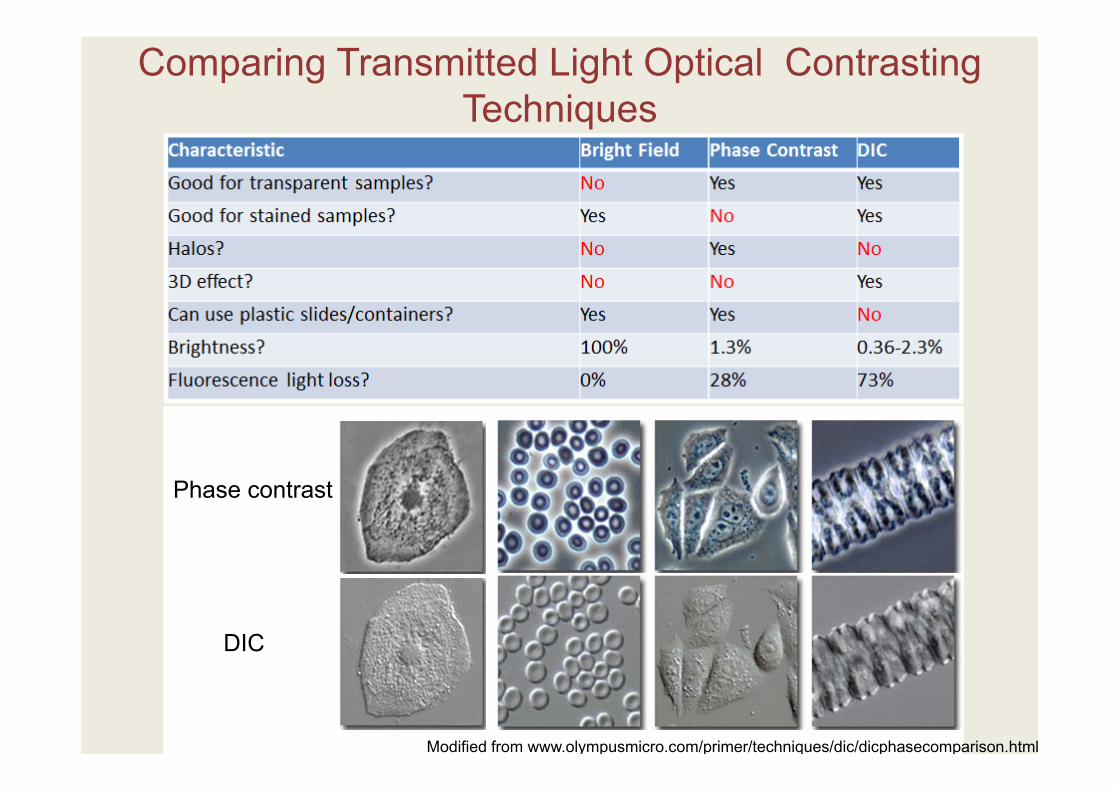
Comparing Transmitted Light Optical Contrasting Techniques
Phase contrast
DIC
Modified from www.olympusmicro.com/primer/techniques/dic/dicphasecomparison.html
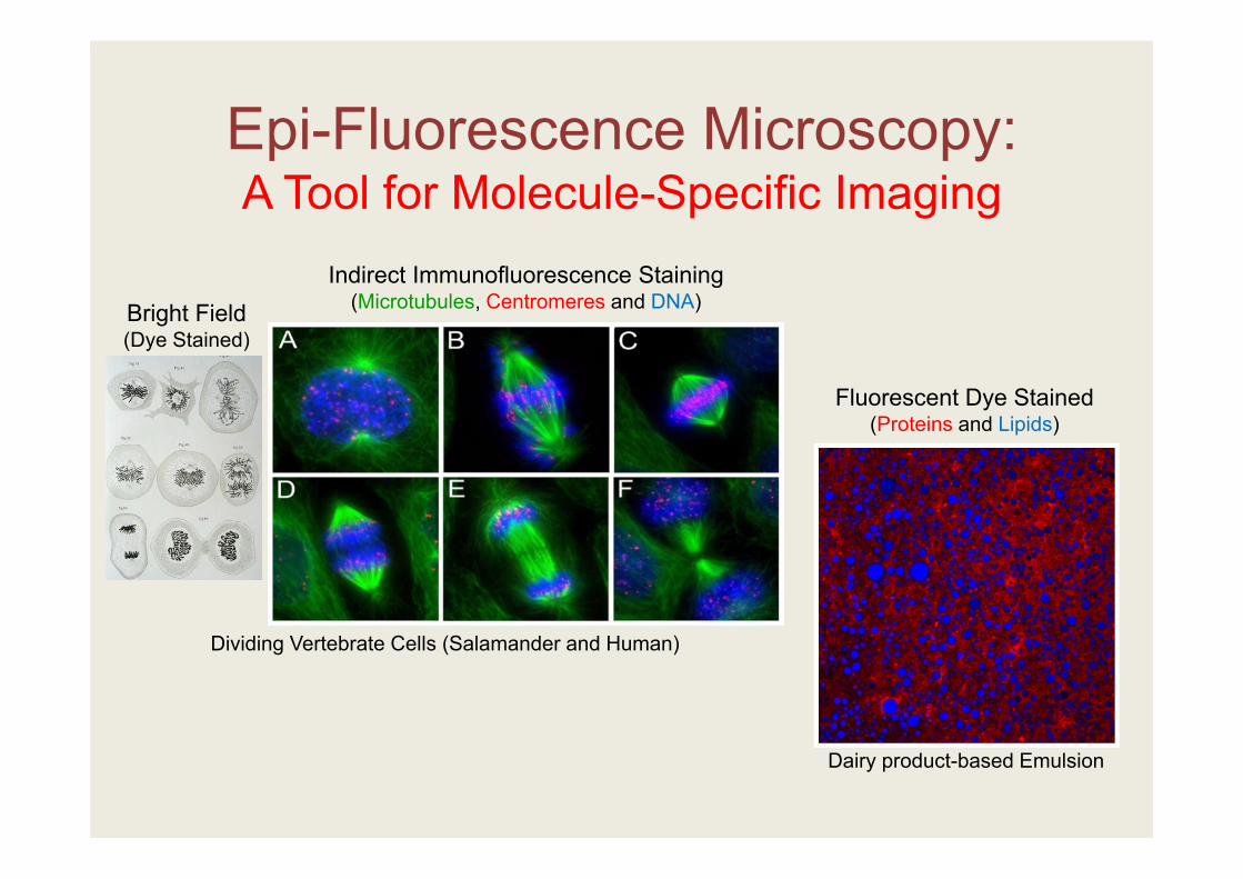
Epi-Fluorescence Microscopy:A Tool for Molecule-Specific Imaging
Bright Field (Dye Stained)
Indirect Immunofluorescence Staining (Microtubules, Centromeres and DNA)
Dividing Vertebrate Cells (Salamander and Human)
Fluorescent Dye Stained (Proteins and Lipids)
Dairy product-based Emulsion
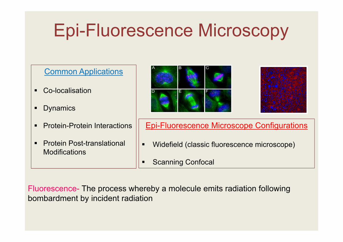
Epi-Fluorescence Microscopy
Common Applications
Co-localisation
Dynamics
Protein-Protein Interactions
Protein Post-translational Modifications
Fluorescence- The process whereby a molecule emits radiation following bombardment by incident radiation
Epi-Fluorescence Microscope Configurations
Widefield (classic fluorescence microscope)
Scanning Confocal
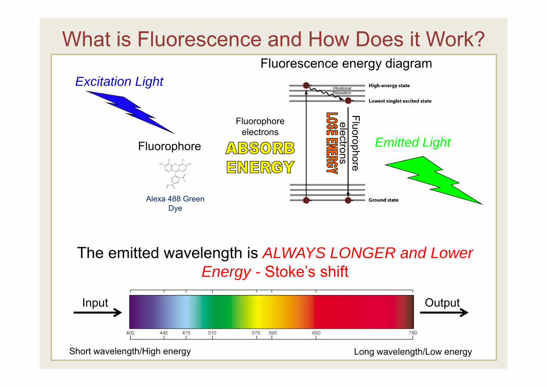
What is Fluorescence and How Does it Work?
Fluorophore
Fluorophoreelectrons
Fluorophoreelectrons
Excitation Light
Emitted Light
Fluorescence energy diagram
GFP
Alexa 488 Green Dye
Vibrational Relaxation
e- e-
e-e-
Long wavelength/Low energyShort wavelength/High energy
The emitted wavelength is ALWAYS LONGER and Lower Energy - Stoke’s shift
Input Output
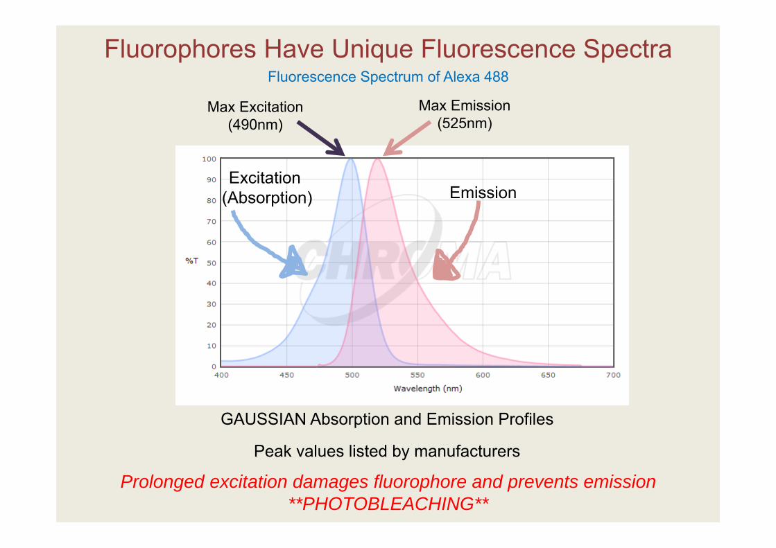
Fluorescence Spectrum of Alexa 488
Excitation(Absorption) Emission
Max Excitation (490nm)
Max Emission (525nm)
Fluorophores Have Unique Fluorescence Spectra
GAUSSIAN Absorption and Emission Profiles
Peak values listed by manufacturers
Prolonged excitation damages fluorophore and prevents emission **PHOTOBLEACHING**
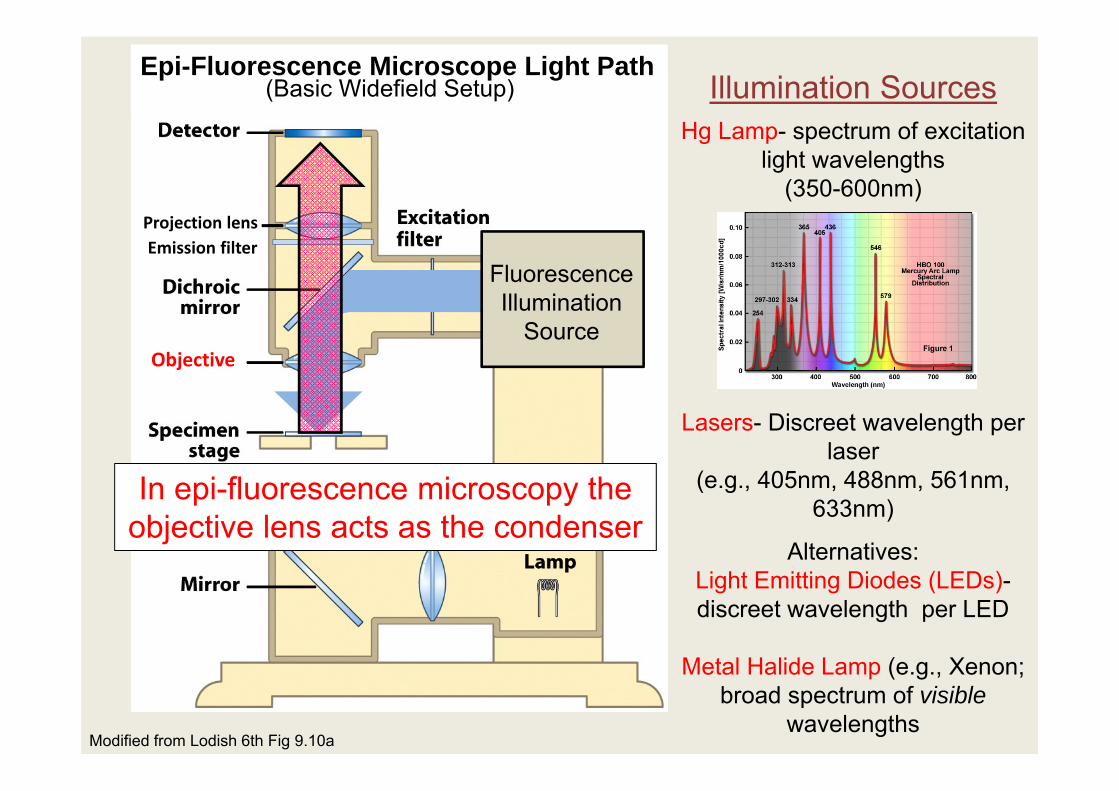
Modified from Lodish 6th Fig 9.10a
Hg Lamp- spectrum of excitation light wavelengths
(350-600nm)
Lasers- Discreet wavelength per laser
(e.g., 405nm, 488nm, 561nm, 633nm)
Alternatives:Light Emitting Diodes (LEDs)-discreet wavelength per LED
Metal Halide Lamp (e.g., Xenon; broad spectrum of visible
wavelengths
Illumination SourcesEpi-Fluorescence Microscope Light Path
Fluorescence Illumination
Source
Projection lensEmission filter
Objective
(Basic Widefield Setup)
In epi-fluorescence microscopy the objective lens acts as the condenser
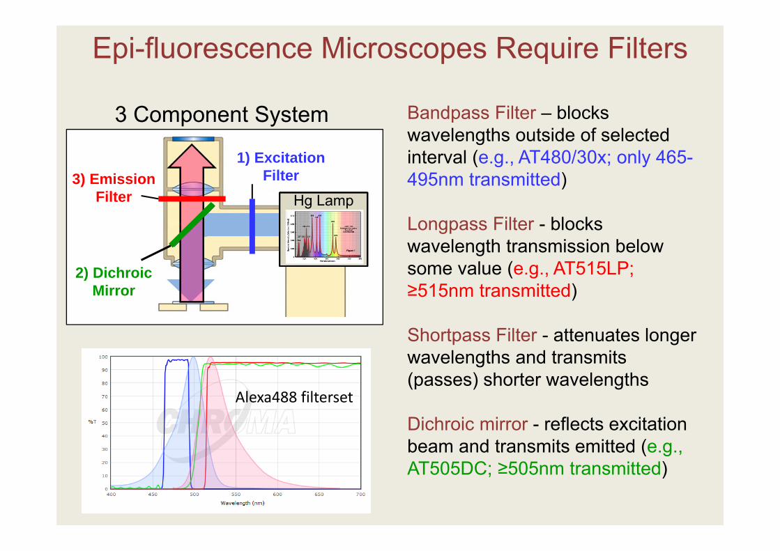
Bandpass Filter – blocks wavelengths outside of selected interval (e.g., AT480/30x; only 465-495nm transmitted)
Longpass Filter - blocks wavelength transmission below some value (e.g., AT515LP; ≥515nm transmitted)
Shortpass Filter - attenuates longer wavelengths and transmits (passes) shorter wavelengths
Dichroic mirror - reflects excitation beam and transmits emitted (e.g., AT505DC; ≥505nm transmitted)
Epi-fluorescence Microscopes Require Filters
3) Emission Filter
1) Excitation Filter
2) Dichroic Mirror
Hg Lamp
3 Component System
Alexa488 filterset
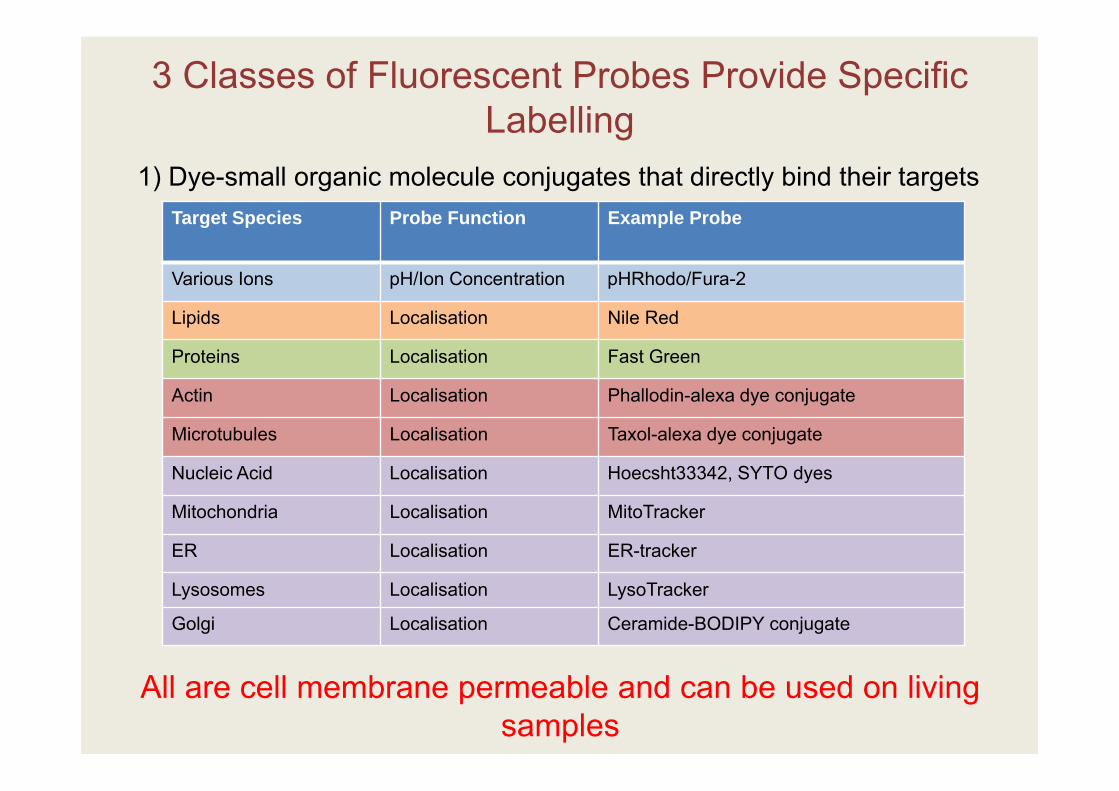
3 Classes of Fluorescent Probes Provide Specific Labelling
Target Species Probe Function Example Probe
Various Ions pH/Ion Concentration pHRhodo/Fura-2
Lipids Localisation Nile Red
Proteins Localisation Fast Green
Actin Localisation Phallodin-alexa dye conjugate
Microtubules Localisation Taxol-alexa dye conjugate
Nucleic Acid Localisation Hoecsht33342, SYTO dyes
Mitochondria Localisation MitoTracker
ER Localisation ER-tracker
Lysosomes Localisation LysoTracker
Golgi Localisation Ceramide-BODIPY conjugate
All are cell membrane permeable and can be used on living samples
1) Dye-small organic molecule conjugates that directly bind their targets
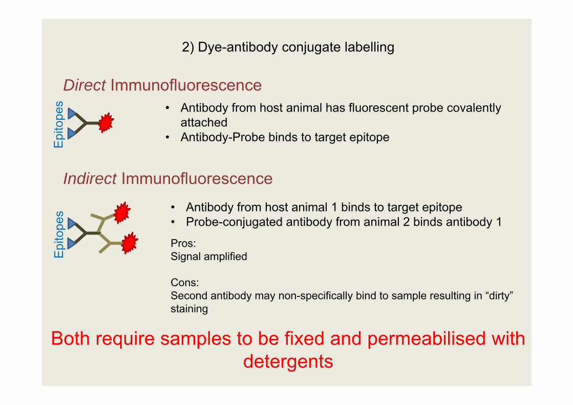
2) Dye-antibody conjugate labelling
Direct Immunofluorescence
Indirect Immunofluorescence
• Antibody from host animal has fluorescent probe covalently attached
• Antibody-Probe binds to target epitope
• Antibody from host animal 1 binds to target epitope• Probe-conjugated antibody from animal 2 binds antibody 1
Epi
tope
s
Pros:Signal amplified
Cons:Second antibody may non-specifically bind to sample resulting in “dirty” staining
Epi
tope
s
Both require samples to be fixed and permeabilised with detergents
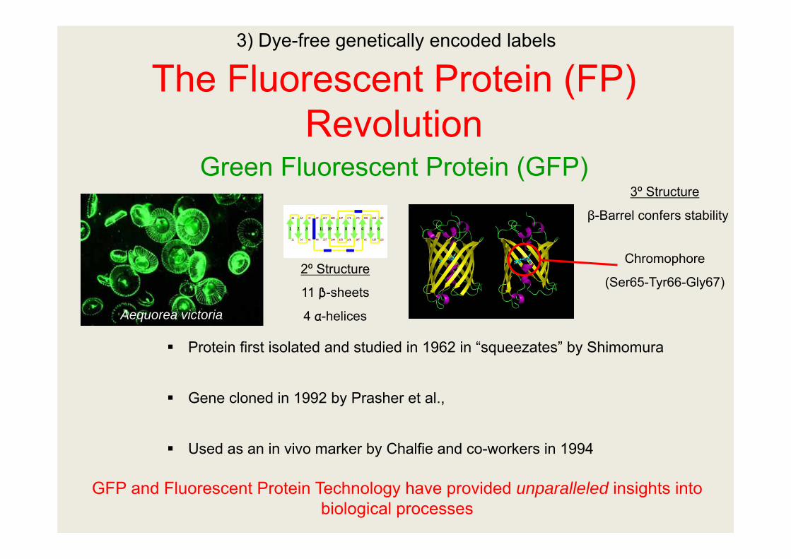
The Fluorescent Protein (FP) Revolution
Green Fluorescent Protein (GFP)
Protein first isolated and studied in 1962 in “squeezates” by Shimomura
Gene cloned in 1992 by Prasher et al.,
Used as an in vivo marker by Chalfie and co-workers in 1994
Aequorea victoria
2º Structure
11 β-sheets
4 α-helices
3º Structure
β-Barrel confers stability
Chromophore
(Ser65-Tyr66-Gly67)
3) Dye-free genetically encoded labels
GFP and Fluorescent Protein Technology have provided unparalleled insights into biological processes
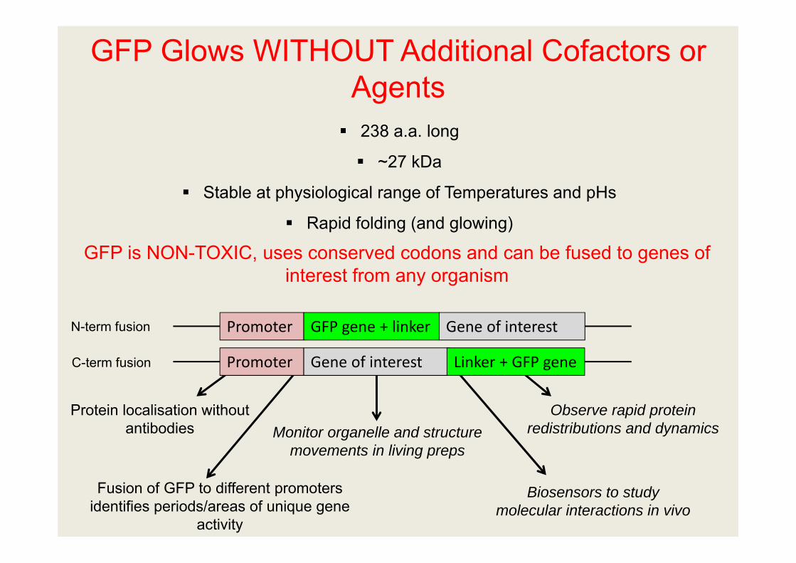
GFP is NON-TOXIC, uses conserved codons and can be fused to genes of interest from any organism
238 a.a. long
~27 kDa
Stable at physiological range of Temperatures and pHs
Rapid folding (and glowing)
GFP Glows WITHOUT Additional Cofactors or Agents
Protein localisation without antibodies Monitor organelle and structure
movements in living preps
Biosensors to study molecular interactions in vivo
Fusion of GFP to different promoters identifies periods/areas of unique gene
activity
Observe rapid protein redistributions and dynamics
Promoter GFP gene + linker Gene of interest
Promoter Gene of interest Linker + GFP gene
N-term fusion
C-term fusion
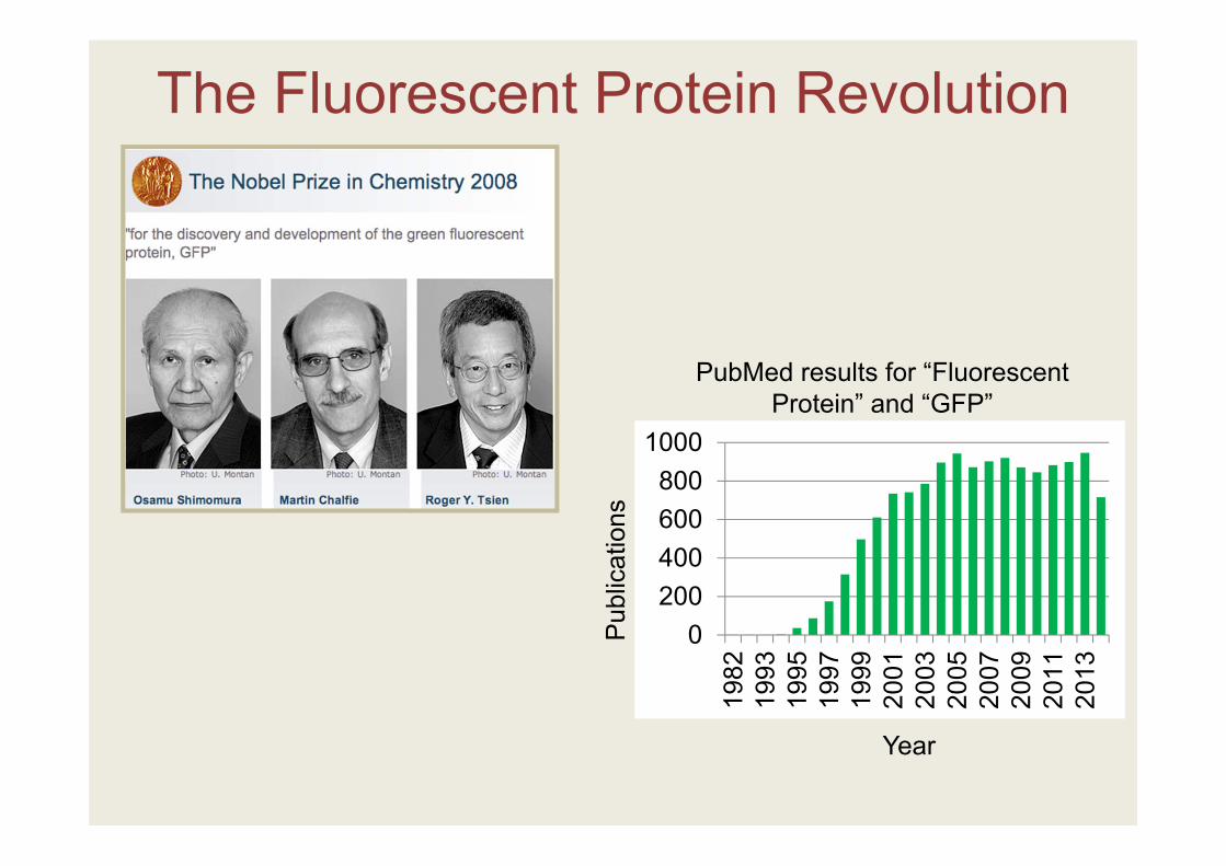
The Fluorescent Protein Revolution
0200400600800
1000
1982
1993
1995
1997
1999
2001
2003
2005
2007
2009
2011
2013
Year
Pub
licat
ions
PubMed results for “Fluorescent Protein” and “GFP”
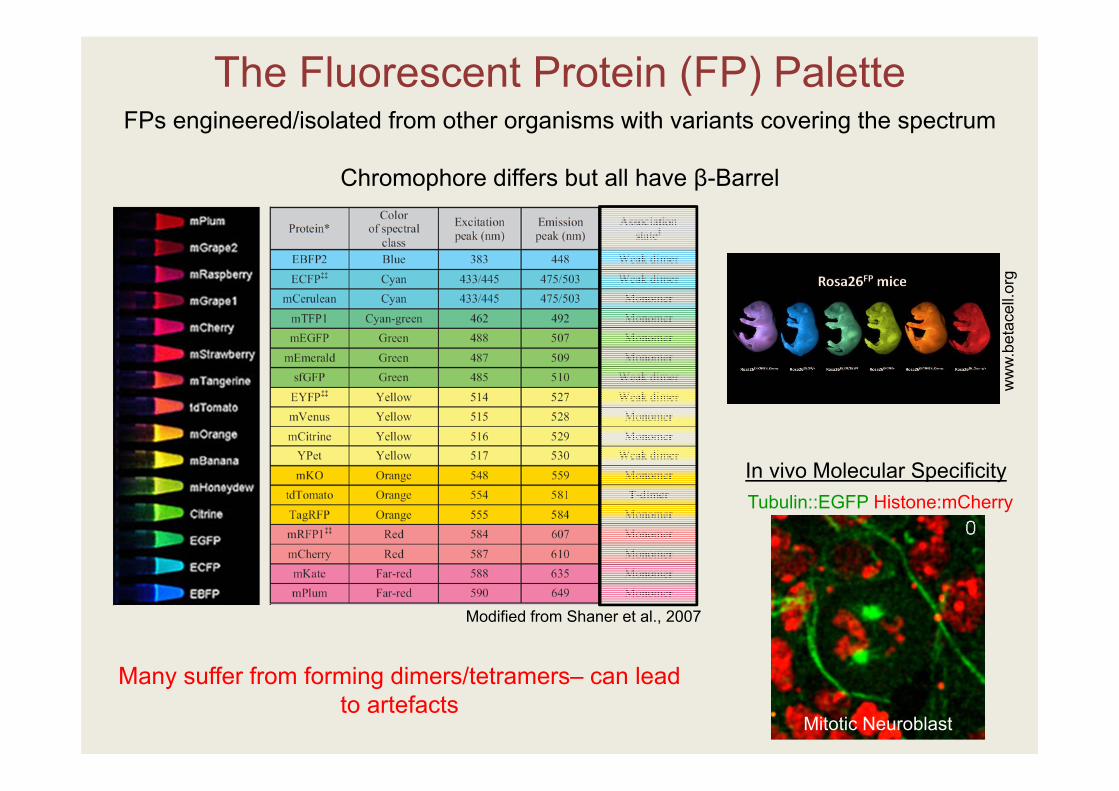
The Fluorescent Protein (FP) Palette
ww
w.be
tace
ll.or
g
FPs engineered/isolated from other organisms with variants covering the spectrum
Chromophore differs but all have β-Barrel
Tubulin::EGFP Histone:mCherry
Mitotic Neuroblast
Modified from Shaner et al., 2007
In vivo Molecular Specificity
Many suffer from forming dimers/tetramers– can lead to artefacts
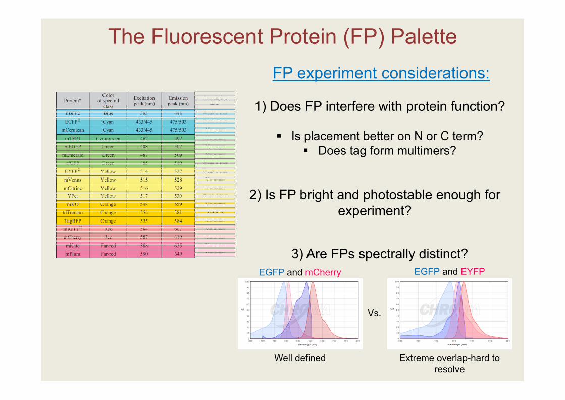
The Fluorescent Protein (FP) PaletteFP experiment considerations:
1) Does FP interfere with protein function?
Is placement better on N or C term? Does tag form multimers?
EGFP and EYFPEGFP and mCherry
Vs.
Well defined Extreme overlap-hard to resolve
3) Are FPs spectrally distinct?
2) Is FP bright and photostable enough for experiment?
Fluorescent Proteins as Optical Highliters
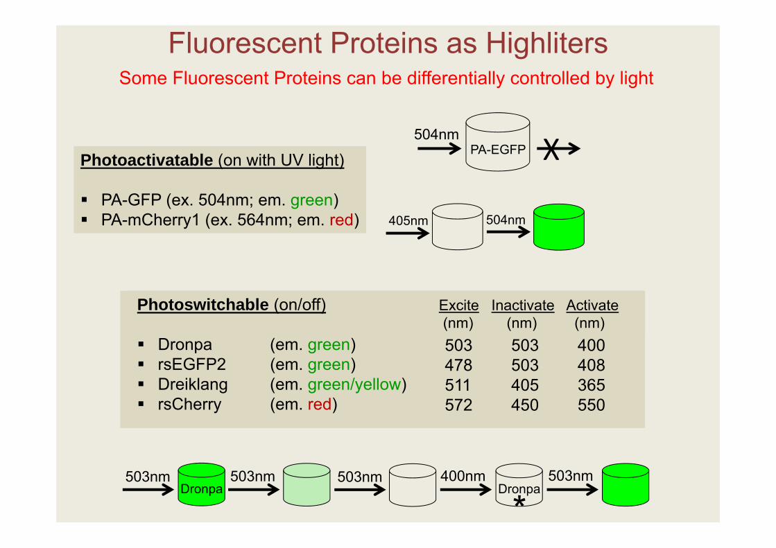
Fluorescent Proteins as Highliters
Photoactivatable (on with UV light)
PA-GFP (ex. 504nm; em. green) PA-mCherry1 (ex. 564nm; em. red)
503nm
*Dronpa
400nmDronpa
503nm503nm 503nm
504nmPA-EGFP X
405nm 504nm
Photoswitchable (on/off)
Dronpa (em. green) rsEGFP2 (em. green) Dreiklang (em. green/yellow) rsCherry (em. red)
503 503 400478 503 408511 405 365572 450 550
Excite Inactivate Activate(nm) (nm) (nm)
Some Fluorescent Proteins can be differentially controlled by light
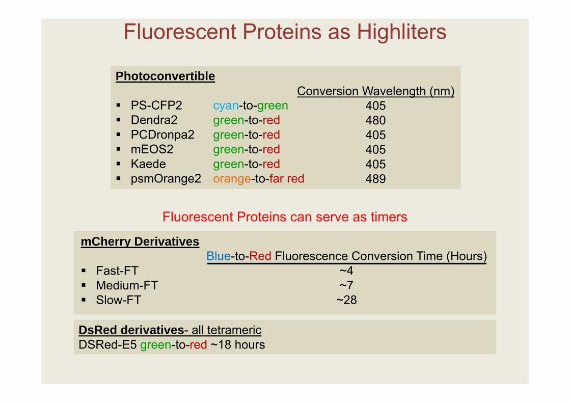
Fluorescent Proteins as Highliters
Fluorescent Proteins can serve as timers
Photoconvertible
PS-CFP2 cyan-to-green Dendra2 green-to-red PCDronpa2 green-to-red mEOS2 green-to-red Kaede green-to-red psmOrange2 orange-to-far red
Conversion Wavelength (nm)405480405405405489
mCherry Derivatives
Fast-FT Medium-FT Slow-FT
DsRed derivatives- all tetramericDSRed-E5 green-to-red ~18 hours
Blue-to-Red Fluorescence Conversion Time (Hours)~4~7~28
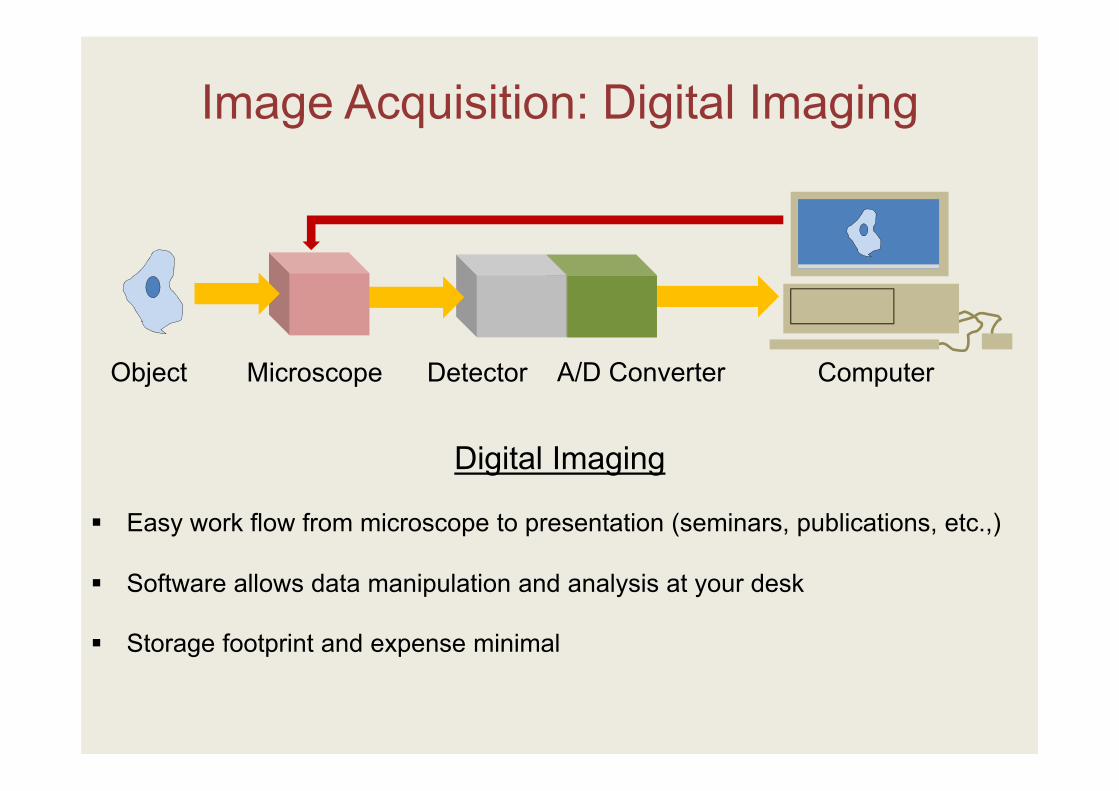
Image Acquisition: Digital Imaging
Object Microscope Detector A/D Converter Computer
Digital Imaging
Easy work flow from microscope to presentation (seminars, publications, etc.,)
Software allows data manipulation and analysis at your desk
Storage footprint and expense minimal
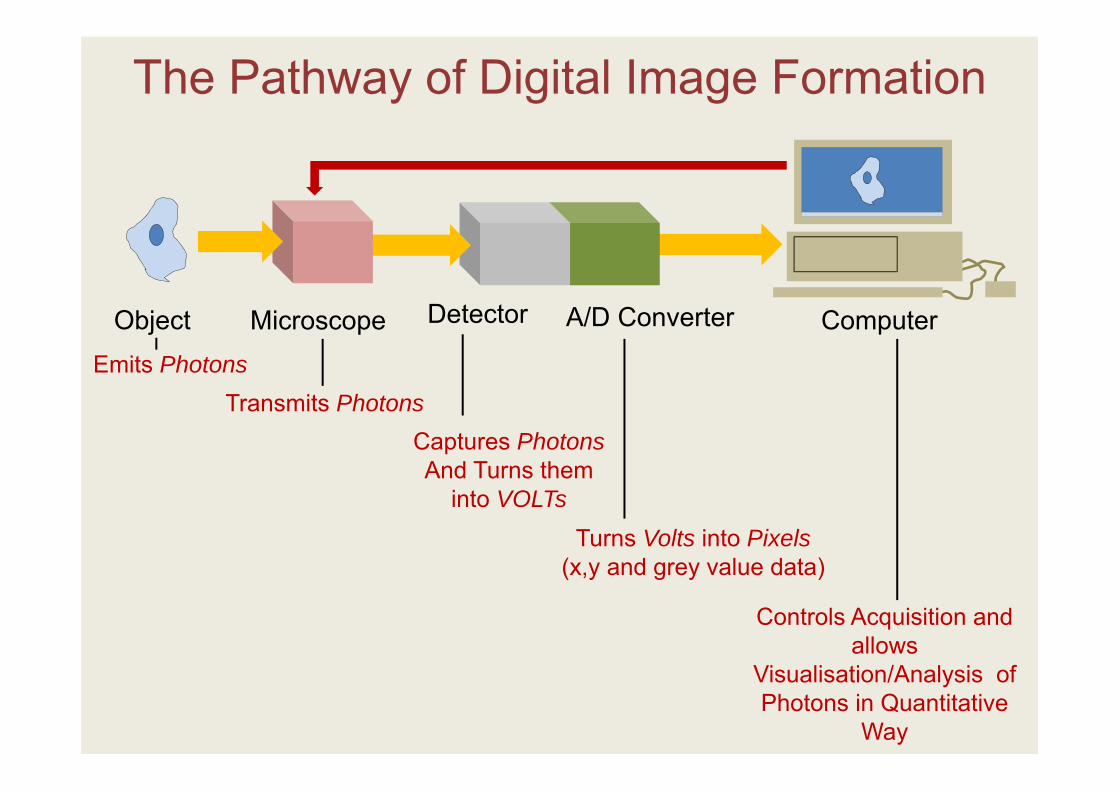
Transmits Photons
Turns Volts into Pixels(x,y and grey value data)
Captures PhotonsAnd Turns them
into VOLTs
Controls Acquisition and allows
Visualisation/Analysis of Photons in Quantitative
Way
Emits Photons
The Pathway of Digital Image Formation
Object Microscope Detector A/D Converter Computer
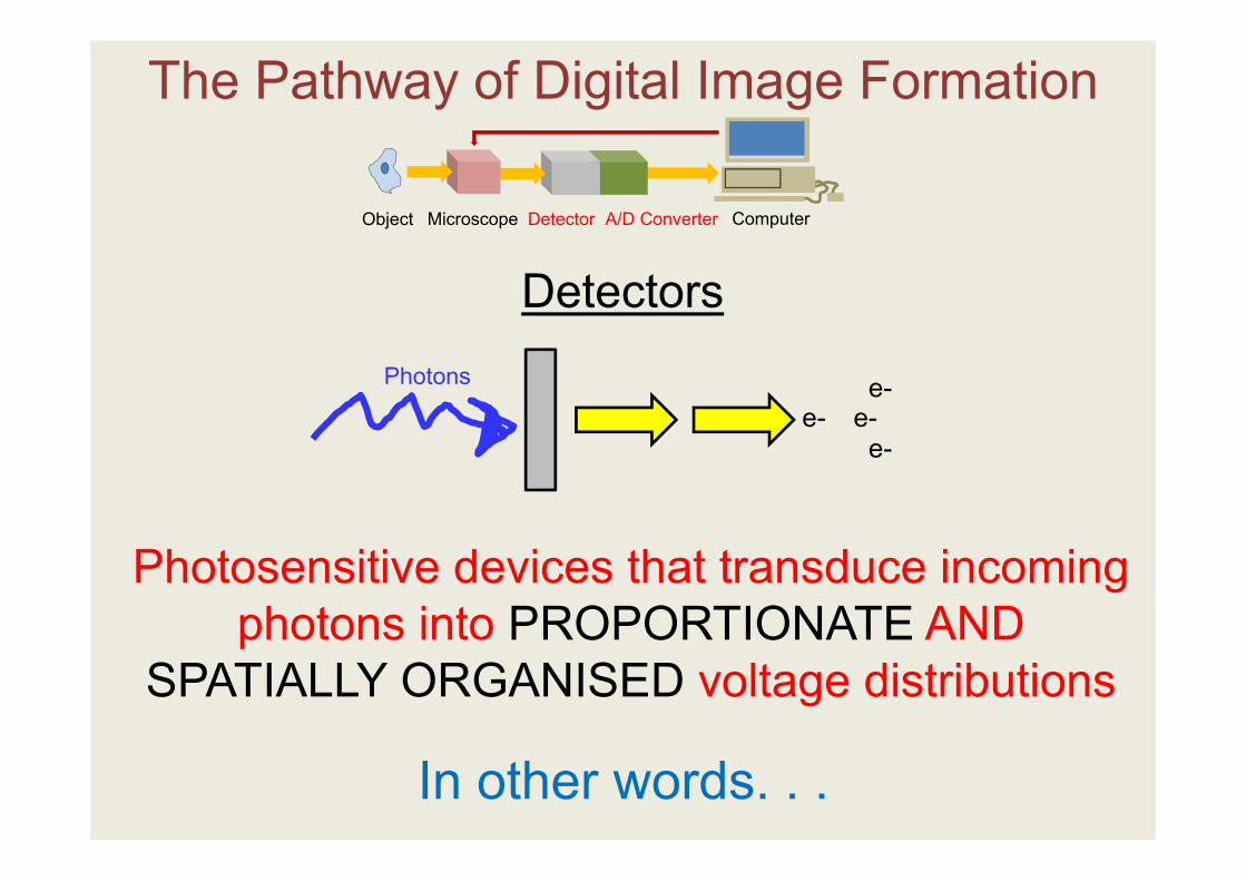
The Pathway of Digital Image Formation
Detectors
Photosensitive devices that transduce incoming photons into PROPORTIONATE AND
SPATIALLY ORGANISED voltage distributions
In other words. . .
Object Microscope Detector A/D Converter Computer
Photons
e- e-e-
e-
X-Axis
Y-A
xis
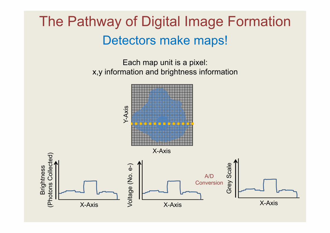
The Pathway of Digital Image FormationDetectors make maps!
X-Axis
Brig
htne
ss
(Pho
tons
Col
lect
ed)
X-AxisVolta
ge (N
o. e
-)
X-Axis
Gre
y S
cale
A/D Conversion
Each map unit is a pixel: x,y information and brightness information
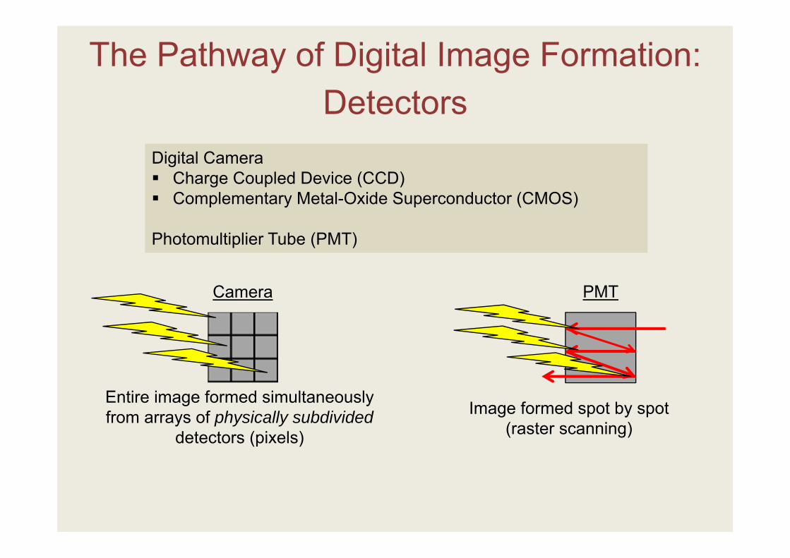
The Pathway of Digital Image Formation:
Digital Camera Charge Coupled Device (CCD) Complementary Metal-Oxide Superconductor (CMOS)
Photomultiplier Tube (PMT)
Detectors
Camera
Entire image formed simultaneously from arrays of physically subdivided
detectors (pixels)
PMT
Image formed spot by spot (raster scanning)
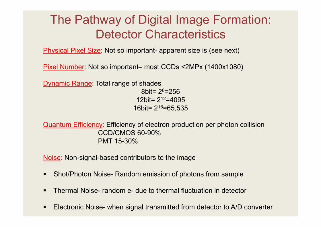
Physical Pixel Size: Not so important- apparent size is (see next)
Pixel Number: Not so important– most CCDs <2MPx (1400x1080)
Dynamic Range: Total range of shades8bit= 28=256
12bit= 212=409516bit= 216=65,535
Quantum Efficiency: Efficiency of electron production per photon collisionCCD/CMOS 60-90%PMT 15-30%
Noise: Non-signal-based contributors to the image
Shot/Photon Noise- Random emission of photons from sample
Thermal Noise- random e- due to thermal fluctuation in detector
Electronic Noise- when signal transmitted from detector to A/D converter
The Pathway of Digital Image Formation: Detector Characteristics
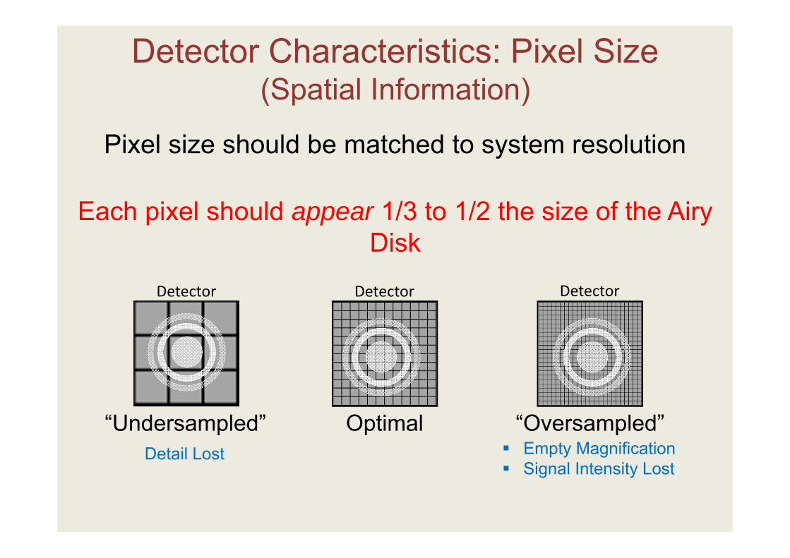
Each pixel should appear 1/3 to 1/2 the size of the Airy Disk
Pixel size should be matched to system resolution
“Undersampled” Optimal “Oversampled”Detail Lost Empty Magnification
Signal Intensity Lost
Detector Detector Detector
Detector Characteristics: Pixel Size (Spatial Information)
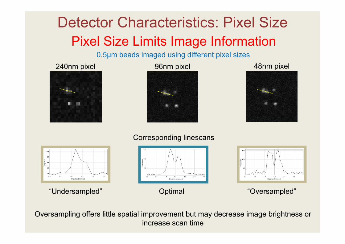
Pixel Size Limits Image Information
“Undersampled” Optimal “Oversampled”
0.5µm beads imaged using different pixel sizes240nm pixel 96nm pixel 48nm pixel
Oversampling offers little spatial improvement but may decrease image brightness or increase scan time
Corresponding linescans
Detector Characteristics: Pixel Size
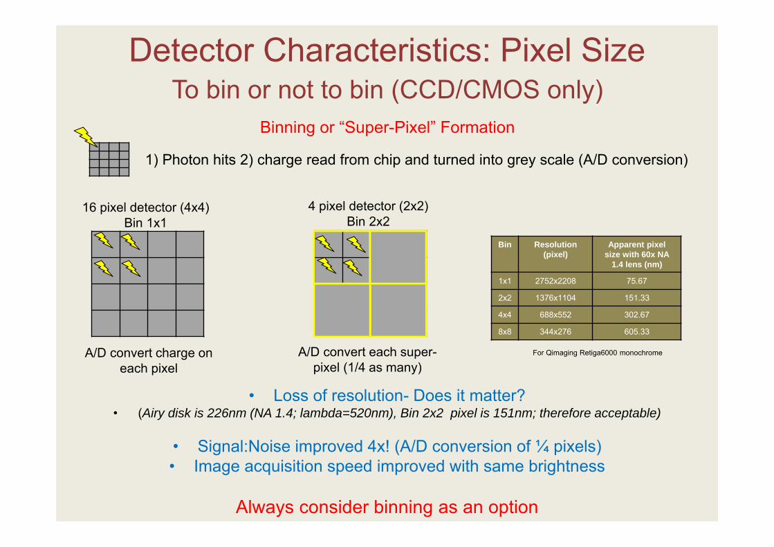
Detector Characteristics: Pixel Size
16 pixel detector (4x4)Bin 1x1
4 pixel detector (2x2)Bin 2x2
To bin or not to bin (CCD/CMOS only)
• Loss of resolution- Does it matter? • (Airy disk is 226nm (NA 1.4; lambda=520nm), Bin 2x2 pixel is 151nm; therefore acceptable)
• Signal:Noise improved 4x! (A/D conversion of ¼ pixels)• Image acquisition speed improved with same brightness
Always consider binning as an option
Binning or “Super-Pixel” Formation
Bin Resolution (pixel)
Apparent pixel size with 60x NA
1.4 lens (nm)
1x1 2752x2208 75.67
2x2 1376x1104 151.33
4x4 688x552 302.67
8x8 344x276 605.33
For Qimaging Retiga6000 monochrome
1) Photon hits 2) charge read from chip and turned into grey scale (A/D conversion)
A/D convert charge on each pixel
A/D convert each super-pixel (1/4 as many)
Detector
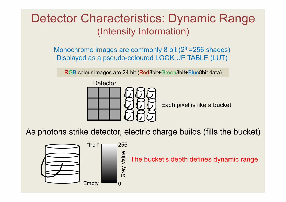
Monochrome images are commonly 8 bit (28 =256 shades)Displayed as a pseudo-coloured LOOK UP TABLE (LUT)
RGB colour images are 24 bit (Red8bit+Green8bit+Blue8bit data)
As photons strike detector, electric charge builds (fills the bucket)
The bucket’s depth defines dynamic range
255
0
Gre
y Va
lue
“Full”
“Empty”
Each pixel is like a bucket
Detector Characteristics: Dynamic Range (Intensity Information)
As photons strike, electric charge PROPORTIONATELY accumulates(fills the bucket)
255
0
Gre
y Va
lue
“Full”
“Empty”e‐
e‐
e‐
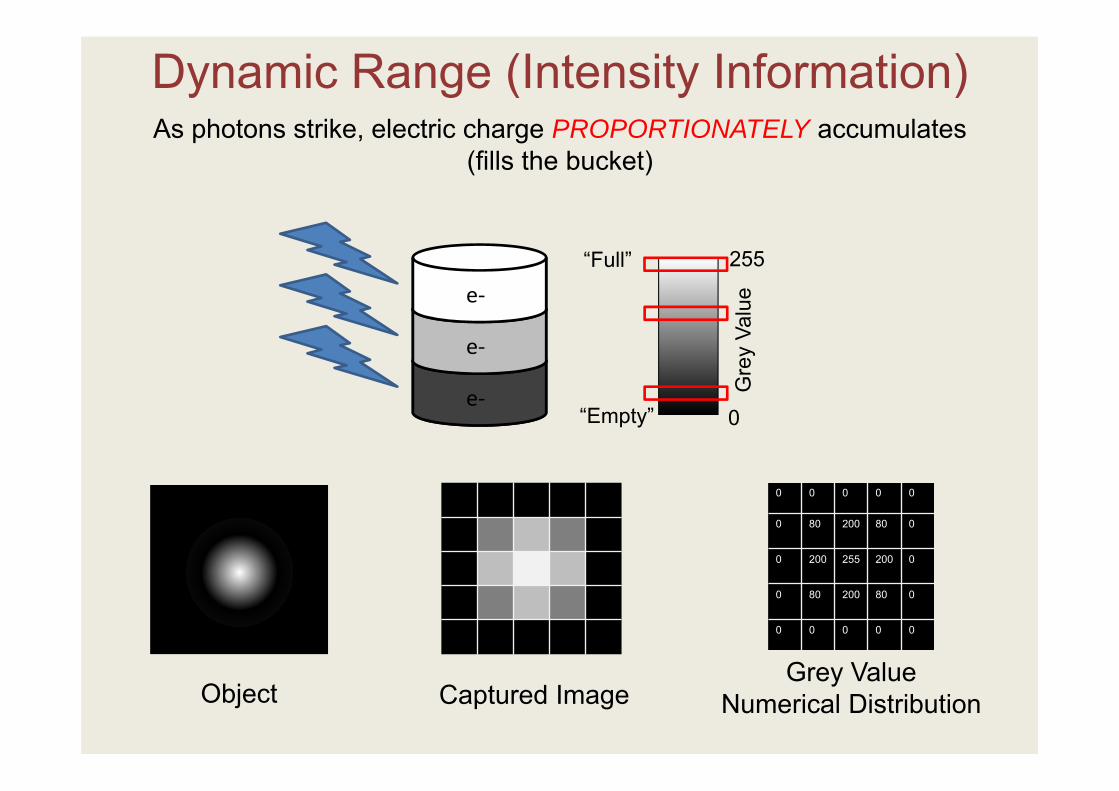
Dynamic Range (Intensity Information)
0 0 0 0 0
0 80 200 80 0
0 200 255 200 0
0 80 200 80 0
0 0 0 0 0
Object Captured ImageGrey Value
Numerical Distribution
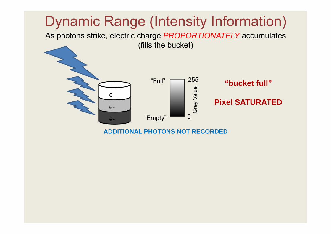
As photons strike, electric charge PROPORTIONATELY accumulates (fills the bucket)
255
0
Gre
y Va
lue
“Full”
“Empty”e‐
e‐
e‐
ADDITIONAL PHOTONS NOT RECORDED
Dynamic Range (Intensity Information)
0 0 0 0 0
0 255 255 255 0
0 255 255 255 0
0 255 255 255 0
0 0 0 0 0
Object Captured ImageGrey Value
Numerical Distribution
“bucket full”
Pixel SATURATED
Adjacent pixels may acquire additional charge and saturate
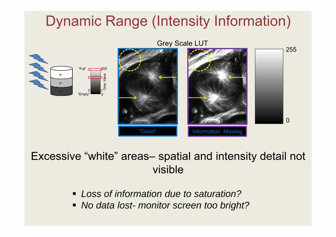
“Good” Information Missing
Grey Scale LUT255
0
Excessive “white” areas– spatial and intensity detail not visible
Loss of information due to saturation? No data lost- monitor screen too bright?
Dynamic Range (Intensity Information)
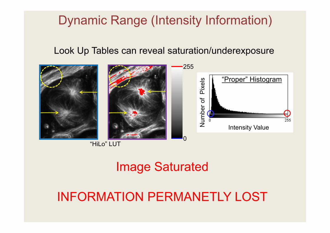
Image Saturated
INFORMATION PERMANETLY LOST
255
0“HiLo” LUT
Dynamic Range (Intensity Information)
“Proper” Histogram
Intensity ValueNum
ber o
f P
ixel
s
Look Up Tables can reveal saturation/underexposure
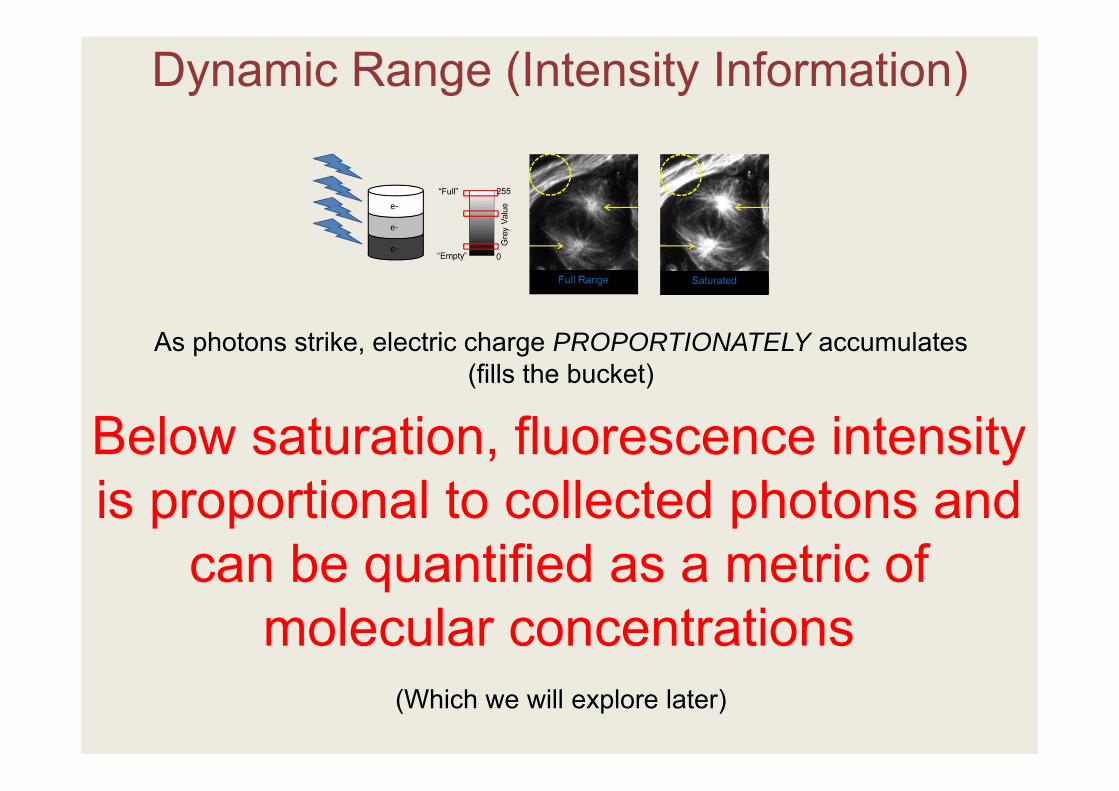
As photons strike, electric charge PROPORTIONATELY accumulates (fills the bucket)
Below saturation, fluorescence intensity is proportional to collected photons and
can be quantified as a metric of molecular concentrations
(Which we will explore later)
Dynamic Range (Intensity Information)
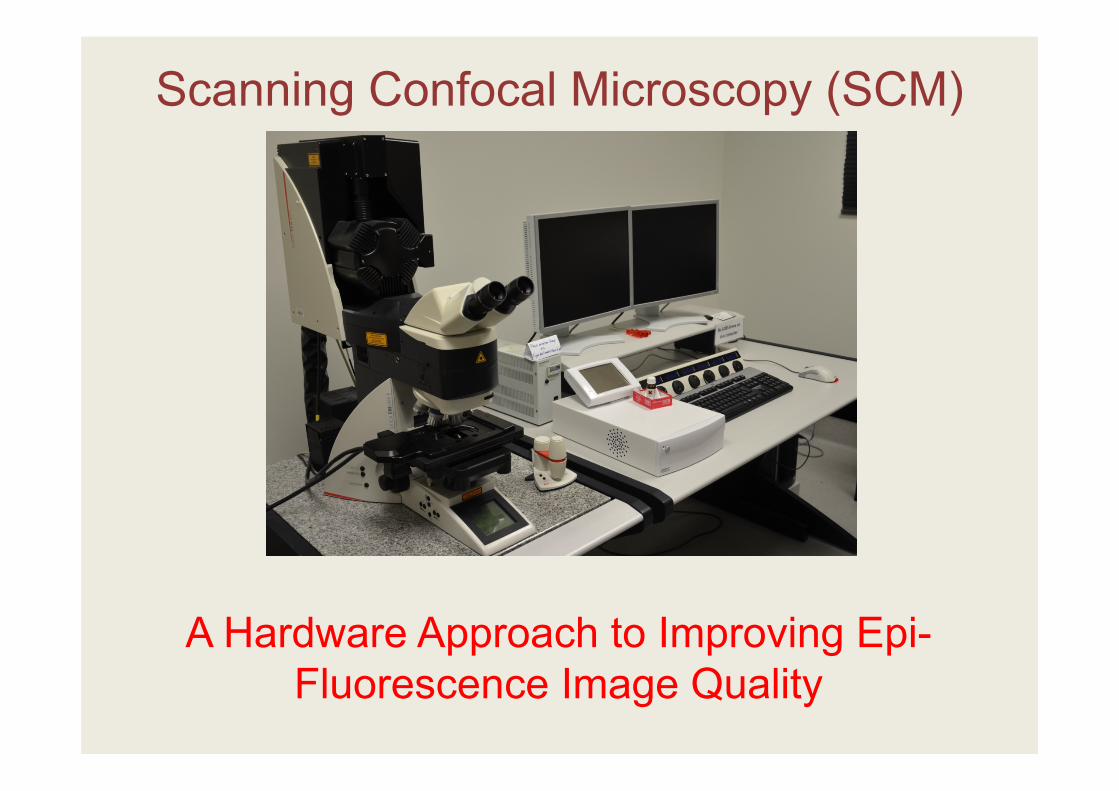
Scanning Confocal Microscopy (SCM)
A Hardware Approach to Improving Epi-Fluorescence Image Quality
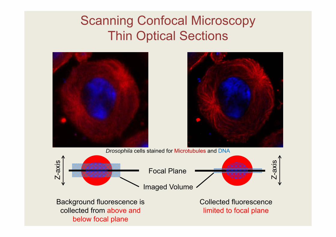
Collected fluorescence limited to focal plane
Background fluorescence is collected from above and
below focal plane
Scanning Confocal MicroscopyThin Optical Sections
Focal Plane
Imaged Volume
Z-ax
is
Z-ax
is
Drosophila cells stained for Microtubules and DNA
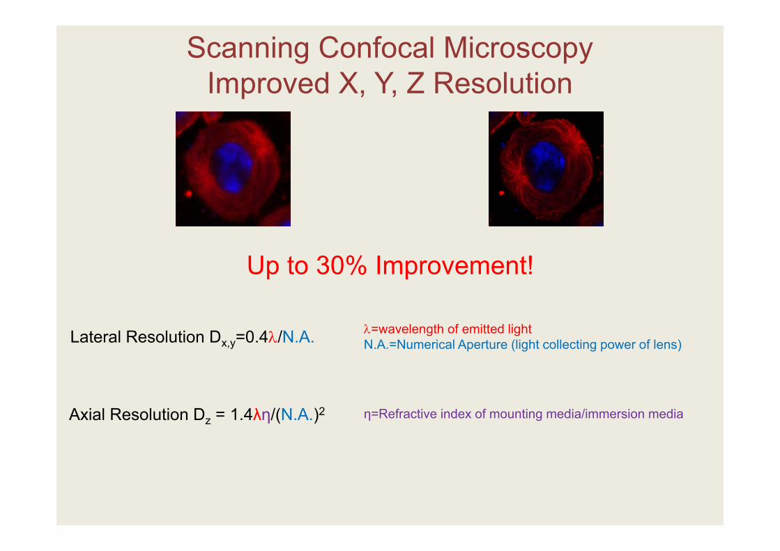
Scanning Confocal MicroscopyImproved X, Y, Z Resolution
Up to 30% Improvement!
=wavelength of emitted lightN.A.=Numerical Aperture (light collecting power of lens)Lateral Resolution Dx,y=0.4/N.A.
Axial Resolution Dz = 1.4λη/(N.A.)2 η=Refractive index of mounting media/immersion media
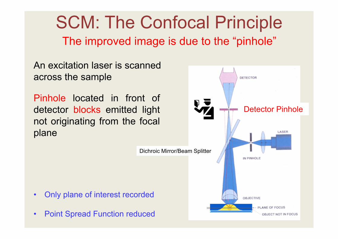
SCM: The Confocal Principle
Pinhole located in front ofdetector blocks emitted lightnot originating from the focalplane
Detector Pinhole
Dichroic Mirror/Beam Splitter
The improved image is due to the “pinhole”
An excitation laser is scanned across the sample
• Only plane of interest recorded
• Point Spread Function reduced
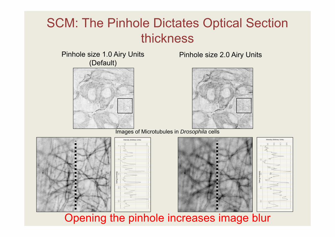
SCM: The Pinhole Dictates Optical Section thickness
Intensity (Arbitrary Units)
Distance (P
ixels)
Distance (P
ixels)
Intensity (Arbitrary Units)
Opening the pinhole increases image blur
Pinhole size 1.0 Airy Units(Default)
Pinhole size 2.0 Airy Units
Images of Microtubules in Drosophila cells
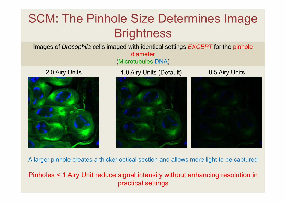
SCM: The Pinhole Size Determines Image Brightness
2.0 Airy Units
Images of Drosophila cells imaged with identical settings EXCEPT for the pinhole diameter
(Microtubules DNA)
A larger pinhole creates a thicker optical section and allows more light to be captured
Pinholes < 1 Airy Unit reduce signal intensity without enhancing resolution in practical settings
0.5 Airy Units1.0 Airy Units (Default)
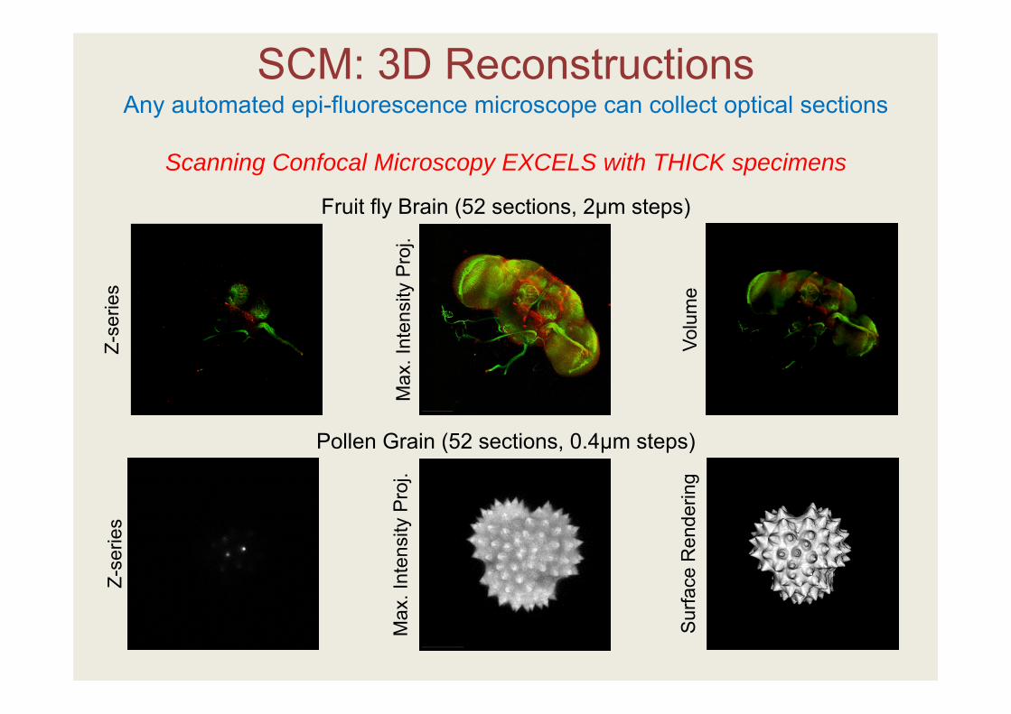
SCM: 3D Reconstructions Any automated epi-fluorescence microscope can collect optical sections
Scanning Confocal Microscopy EXCELS with THICK specimens
Fruit fly Brain (52 sections, 2µm steps)
Pollen Grain (52 sections, 0.4µm steps)
Z-se
ries
Z-se
ries
Max
. Int
ensi
ty P
roj.
Max
. Int
ensi
ty P
roj.
Sur
face
Ren
derin
gVo
lum
e
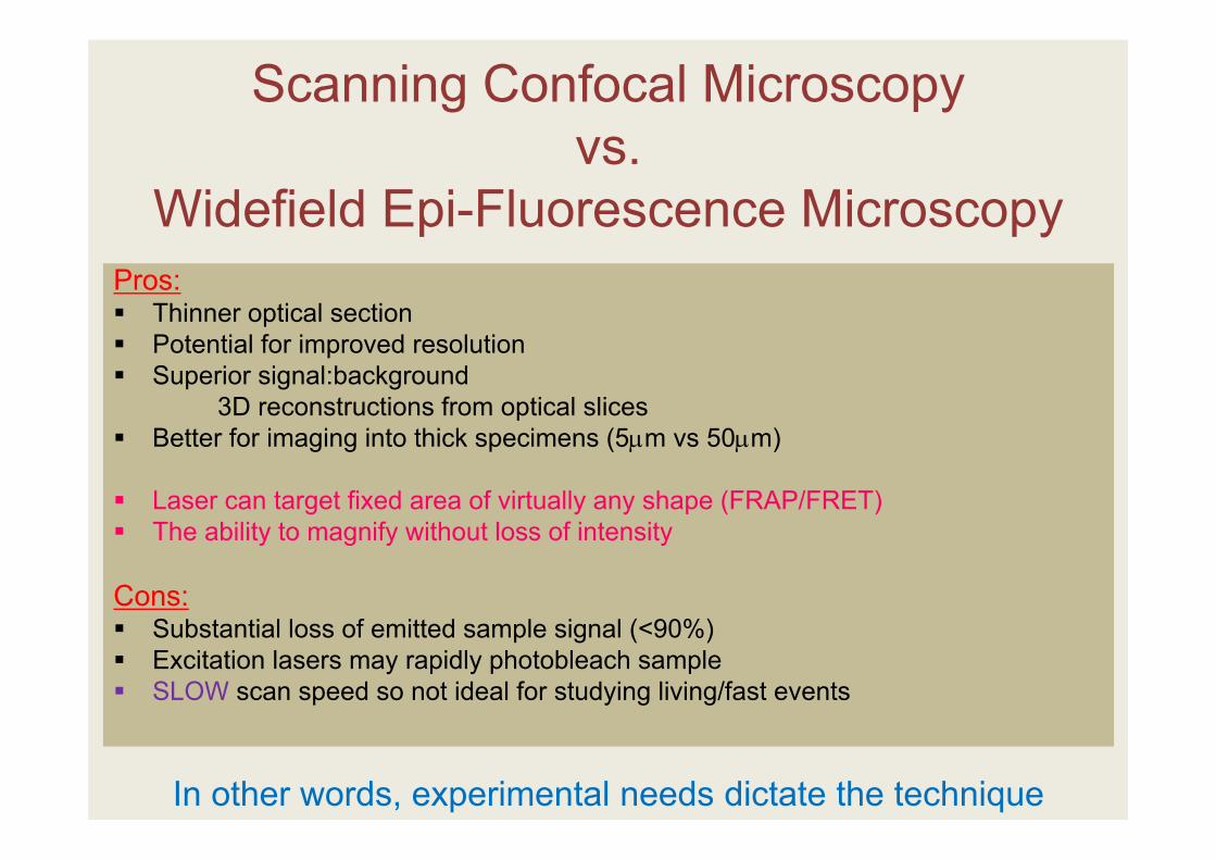
Scanning Confocal Microscopyvs.
Widefield Epi-Fluorescence MicroscopyPros: Thinner optical section Potential for improved resolution Superior signal:background
3D reconstructions from optical slices Better for imaging into thick specimens (5m vs 50m)
Laser can target fixed area of virtually any shape (FRAP/FRET) The ability to magnify without loss of intensity
Cons: Substantial loss of emitted sample signal (<90%) Excitation lasers may rapidly photobleach sample SLOW scan speed so not ideal for studying living/fast events
In other words, experimental needs dictate the technique
More than “pretty pictures”:Light Microscopy As A
Quantitative Tool
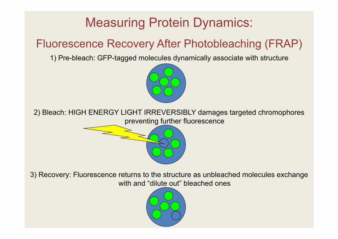
Measuring Protein Dynamics:Fluorescence Recovery After Photobleaching (FRAP)
1) Pre-bleach: GFP-tagged molecules dynamically associate with structure
2) Bleach: HIGH ENERGY LIGHT IRREVERSIBLY damages targeted chromophores preventing further fluorescence
3) Recovery: Fluorescence returns to the structure as unbleached molecules exchange with and “dilute out” bleached ones
Fluo
resc
ence
Inte
nsity
(Arb
itrar
y U
nits
)
Bleach event
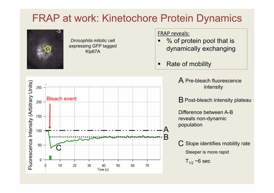
FRAP at work: Kinetochore Protein Dynamics
Pre-bleach fluorescence intensity
Drosophila mitotic cell expressing GFP tagged
Klp67A
Slope identifies mobility rateSteeper is more rapid
T1/2 ~6 sec
Post-bleach intensity plateau
FRAP reveals: % of protein pool that is
dynamically exchanging
Rate of mobility
A
A
B
B
C C
Difference between A-B reveals non-dynamic population
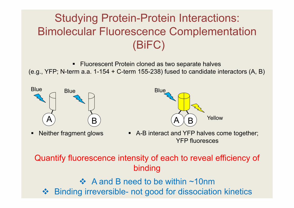
Studying Protein-Protein Interactions: Bimolecular Fluorescence Complementation
(BiFC)
YellowA BA B
Fluorescent Protein cloned as two separate halves (e.g., YFP; N-term a.a. 1-154 + C-term 155-238) fused to candidate interactors (A, B)
Neither fragment glows A-B interact and YFP halves come together; YFP fluoresces
Blue Blue Blue
A and B need to be within ~10nm Binding irreversible- not good for dissociation kinetics
Quantify fluorescence intensity of each to reveal efficiency of binding
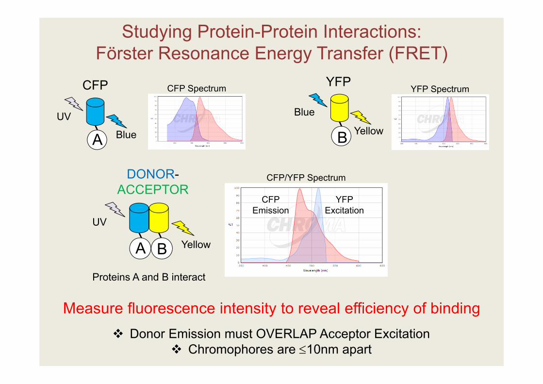
Studying Protein-Protein Interactions:Förster Resonance Energy Transfer (FRET)
A B
UV
Yellow
AUV
Blue
CFP
Proteins A and B interact
YFP
B
Blue
Yellow
Donor Emission must OVERLAP Acceptor Excitation Chromophores are 10nm apart
DONOR-ACCEPTOR
CFP Spectrum YFP Spectrum
CFPEmission
YFPExcitation
CFP/YFP Spectrum
Measure fluorescence intensity to reveal efficiency of binding
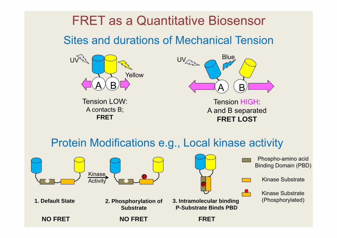
FRET as a Quantitative BiosensorSites and durations of Mechanical Tension
Protein Modifications e.g., Local kinase activity Phospho-amino acid
Binding Domain (PBD)
Kinase Substrate
Kinase Substrate (Phosphorylated)1. Default State
PP
Kinase Activity
2. Phosphorylation of Substrate
3. Intramolecular bindingP-Substrate Binds PBD
NO FRET NO FRET FRET
A B
UV
Yellow
A B
UV
Tension HIGH:A and B separated
FRET LOST
Tension LOW:A contacts B;
FRET
Blue
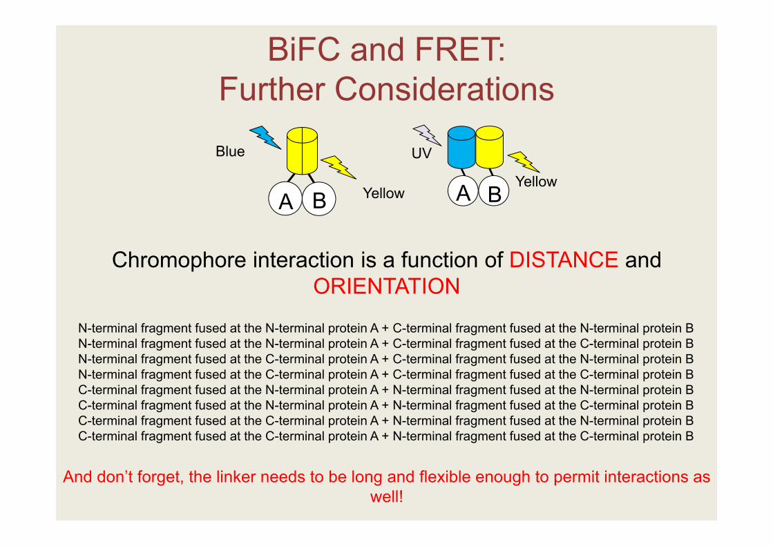
BiFC and FRET:Further Considerations
A B
UV
YellowYellowA B
Chromophore interaction is a function of DISTANCE and ORIENTATION
N-terminal fragment fused at the N-terminal protein A + C-terminal fragment fused at the N-terminal protein BN-terminal fragment fused at the N-terminal protein A + C-terminal fragment fused at the C-terminal protein BN-terminal fragment fused at the C-terminal protein A + C-terminal fragment fused at the N-terminal protein BN-terminal fragment fused at the C-terminal protein A + C-terminal fragment fused at the C-terminal protein BC-terminal fragment fused at the N-terminal protein A + N-terminal fragment fused at the N-terminal protein BC-terminal fragment fused at the N-terminal protein A + N-terminal fragment fused at the C-terminal protein BC-terminal fragment fused at the C-terminal protein A + N-terminal fragment fused at the N-terminal protein BC-terminal fragment fused at the C-terminal protein A + N-terminal fragment fused at the C-terminal protein B
And don’t forget, the linker needs to be long and flexible enough to permit interactions as well!
Blue
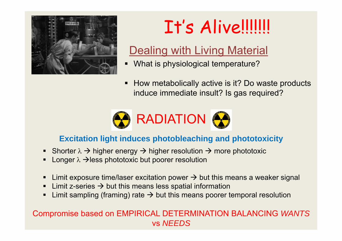
It’s Alive!!!!!!!
What is physiological temperature?
How metabolically active is it? Do waste products induce immediate insult? Is gas required?
Excitation light induces photobleaching and phototoxicity
RADIATION
Shorter higher energy higher resolution more phototoxic Longer less phototoxic but poorer resolution
Limit exposure time/laser excitation power but this means a weaker signal Limit z-series but this means less spatial information Limit sampling (framing) rate but this means poorer temporal resolution
Compromise based on EMPIRICAL DETERMINATION BALANCING WANTSvs NEEDS
Dealing with Living Material

Useful Online References and Primers:
http://www.microscopyu.com/http://zeiss-campus.magnet.fsu.edu/index.html
http://www.olympusmicro.com/index.html
Online spectra comparisonhttp://www.chroma.com/spectra-viewer
Questions?
LUNCH TIME!

ImageJ: A Free to Use Image Analysis Programme
http://imagej.nih.gov/ij/
If you have questions. . . ASK!
There are multiple routes to analysing data
By Wayne Rasband
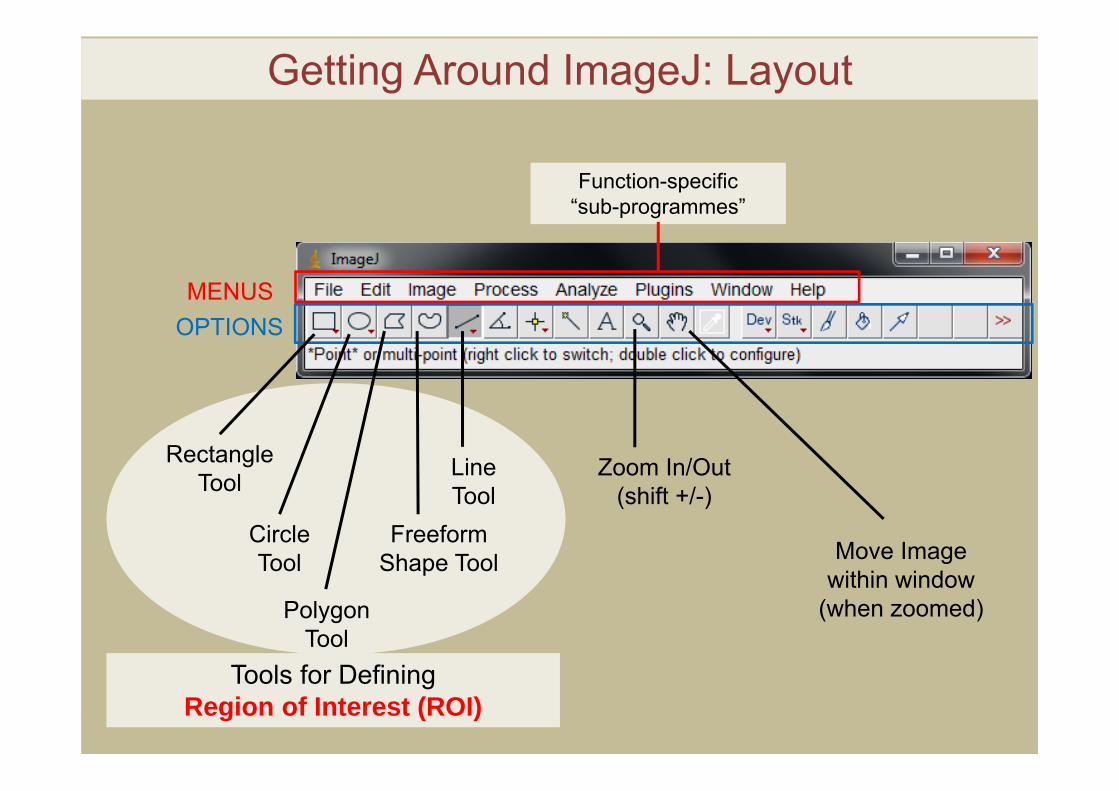
Getting Around ImageJ: Layout
MENUSOPTIONS
RectangleTool
CircleTool
PolygonTool
Line Tool
FreeformShape Tool
Zoom In/Out(shift +/-)
Tools for DefiningRegion of Interest (ROI)
Move Image within window
(when zoomed)
Function-specific “sub-programmes”
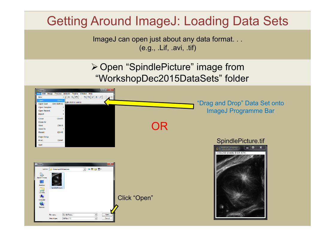
Getting Around ImageJ: Loading Data Sets
“Drag and Drop” Data Set onto ImageJ Programme Bar
Open “SpindlePicture” image from “WorkshopDec2015DataSets” folder
Click “Open”
ORSpindlePicture.tif
ImageJ can open just about any data format. . .(e.g., .Lif, .avi, .tif)
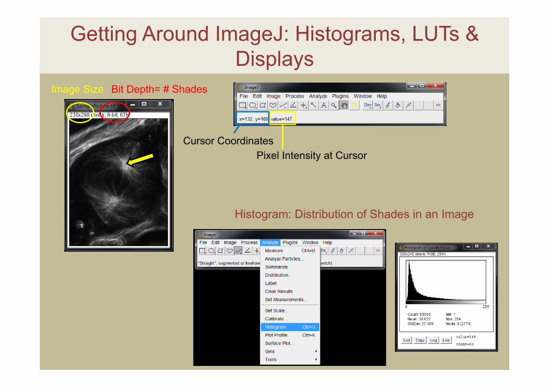
Getting Around ImageJ: Histograms, LUTs & Displays
Histogram: Distribution of Shades in an Image
Image Size Bit Depth= # Shades
Cursor CoordinatesPixel Intensity at Cursor
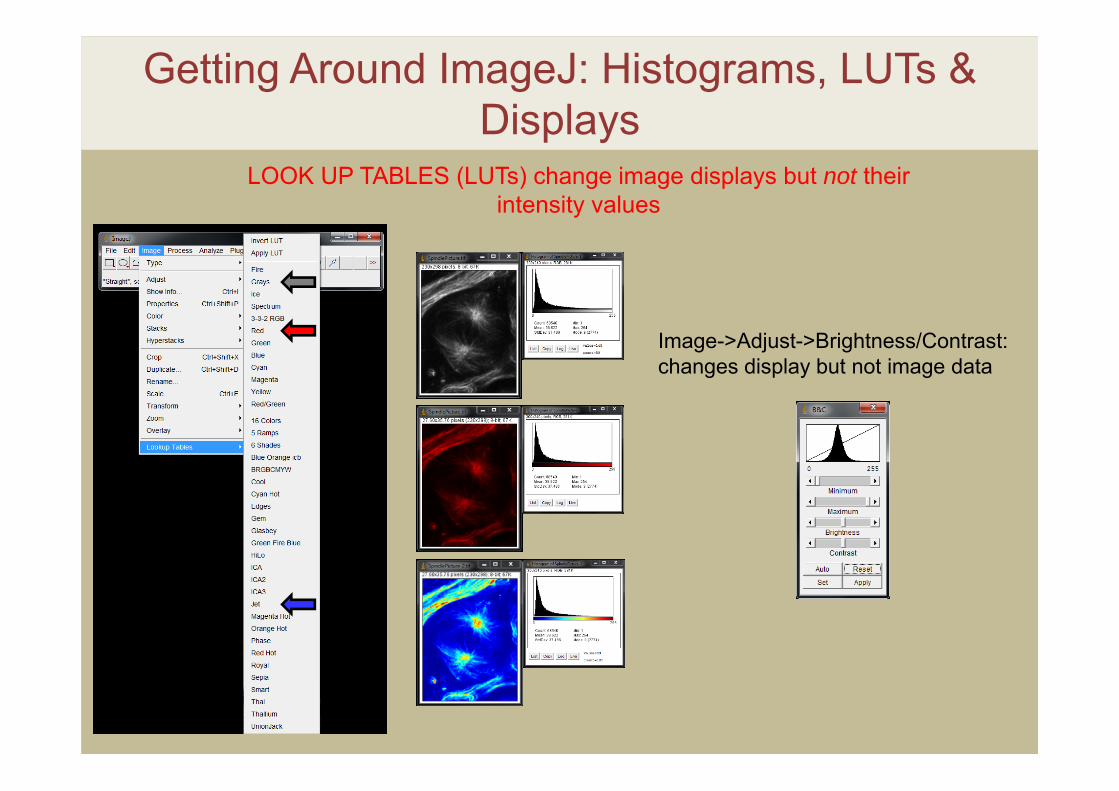
Getting Around ImageJ: Histograms, LUTs & Displays
LOOK UP TABLES (LUTs) change image displays but not their intensity values
Image->Adjust->Brightness/Contrast: changes display but not image data
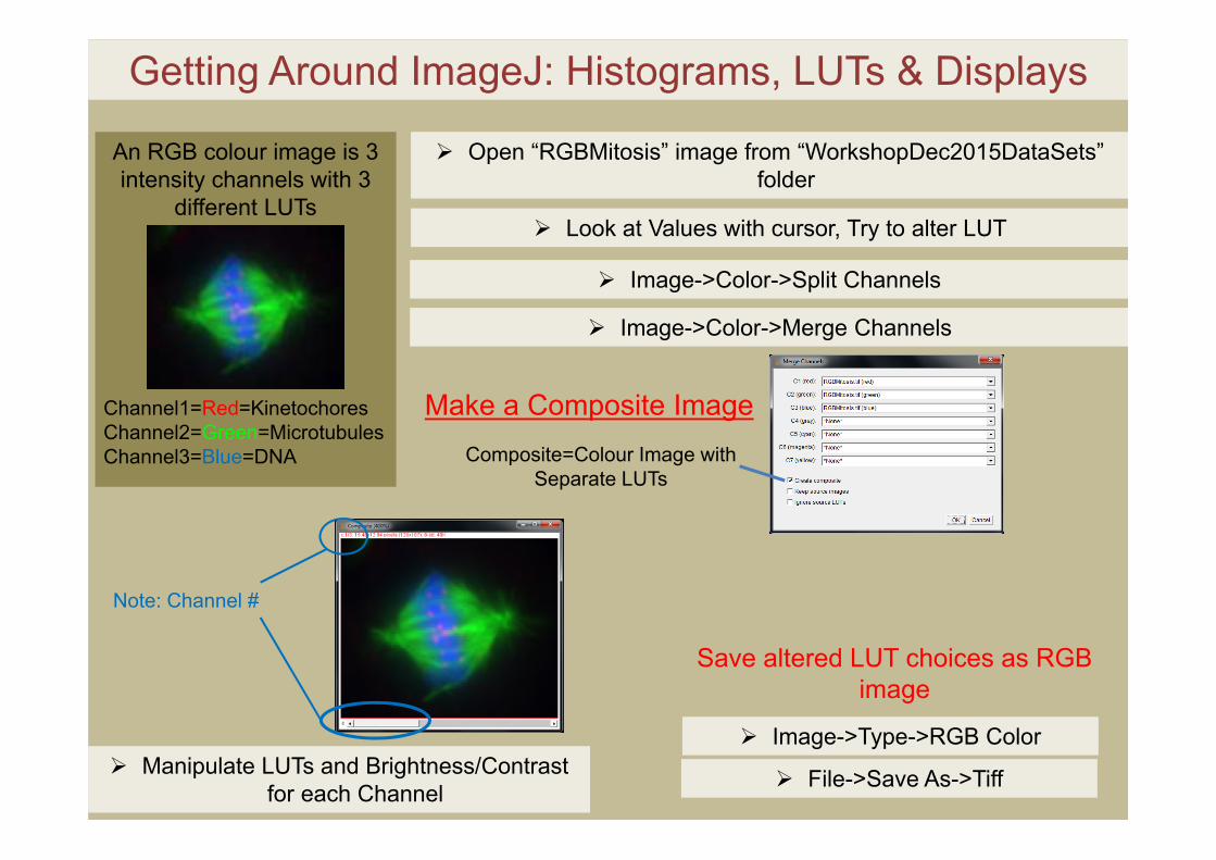
Getting Around ImageJ: Histograms, LUTs & Displays
Open “RGBMitosis” image from “WorkshopDec2015DataSets” folder
Look at Values with cursor, Try to alter LUT
Image->Color->Merge Channels
An RGB colour image is 3 intensity channels with 3
different LUTs
Channel1=Red=KinetochoresChannel2=Green=MicrotubulesChannel3=Blue=DNA Composite=Colour Image with
Separate LUTs
Image->Color->Split Channels
Make a Composite Image
Note: Channel #
Manipulate LUTs and Brightness/Contrast for each Channel
Save altered LUT choices as RGB image
Image->Type->RGB Color
File->Save As->Tiff
Getting Around ImageJ: Histograms, LUTs & Displays
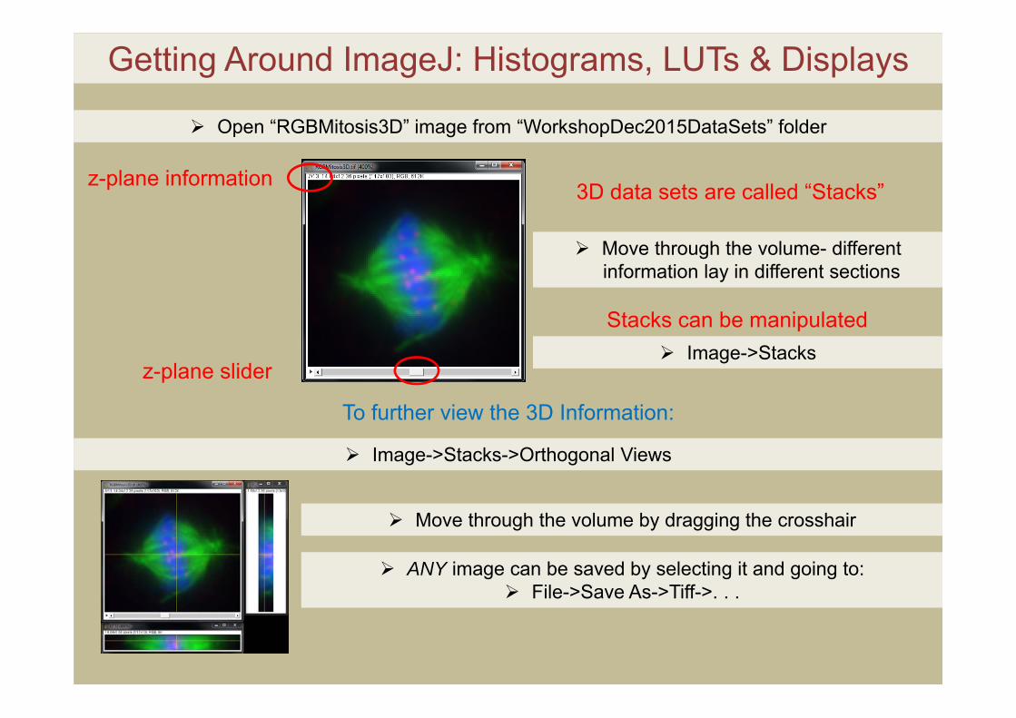
Open “RGBMitosis3D” image from “WorkshopDec2015DataSets” folder
z-plane information
z-plane slider
Move through the volume- different information lay in different sections
To further view the 3D Information:
Image->Stacks->Orthogonal Views
Move through the volume by dragging the crosshair
ANY image can be saved by selecting it and going to: File->Save As->Tiff->. . .
3D data sets are called “Stacks”
Stacks can be manipulated Image->Stacks
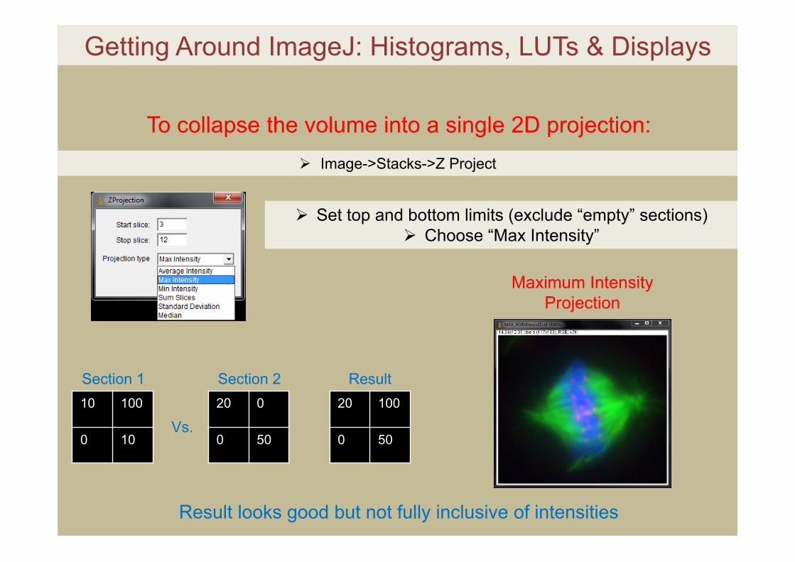
Getting Around ImageJ: Histograms, LUTs & Displays
Image->Stacks->Z Project
To collapse the volume into a single 2D projection:
Set top and bottom limits (exclude “empty” sections) Choose “Max Intensity”
Result looks good but not fully inclusive of intensities
10 100
0 10
20 0
0 50
20 100
0 50
Section 1 Section 2 Result
Vs.
Maximum Intensity Projection
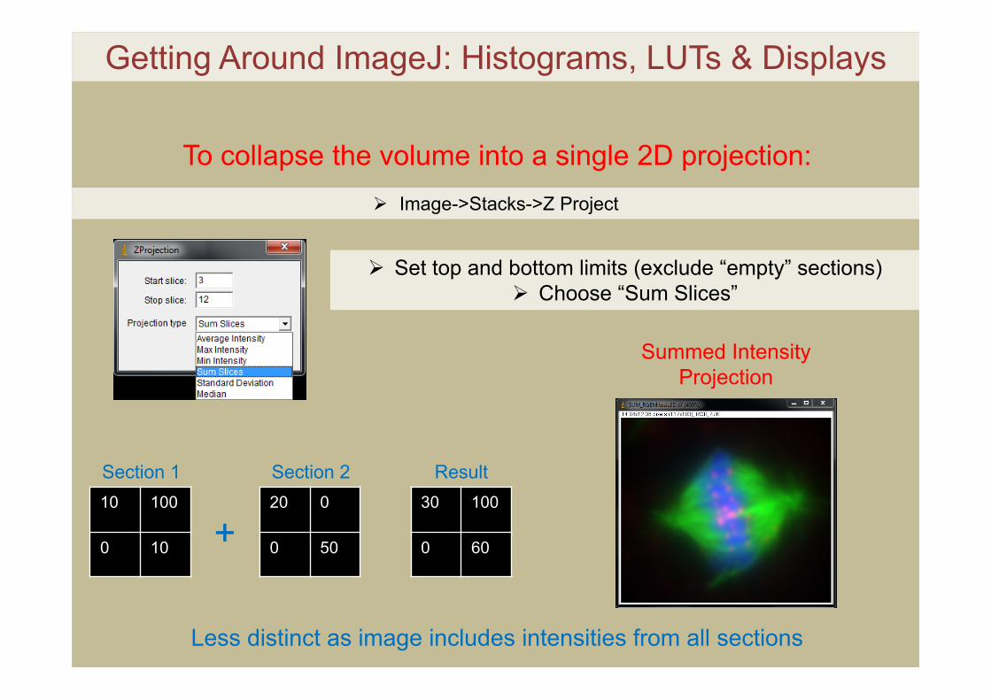
Getting Around ImageJ: Histograms, LUTs & Displays
Image->Stacks->Z Project
To collapse the volume into a single 2D projection:
Set top and bottom limits (exclude “empty” sections) Choose “Sum Slices”
Less distinct as image includes intensities from all sections
10 100
0 10
20 0
0 50
30 100
0 60
Section 1 Section 2 Result
+
Summed Intensity Projection
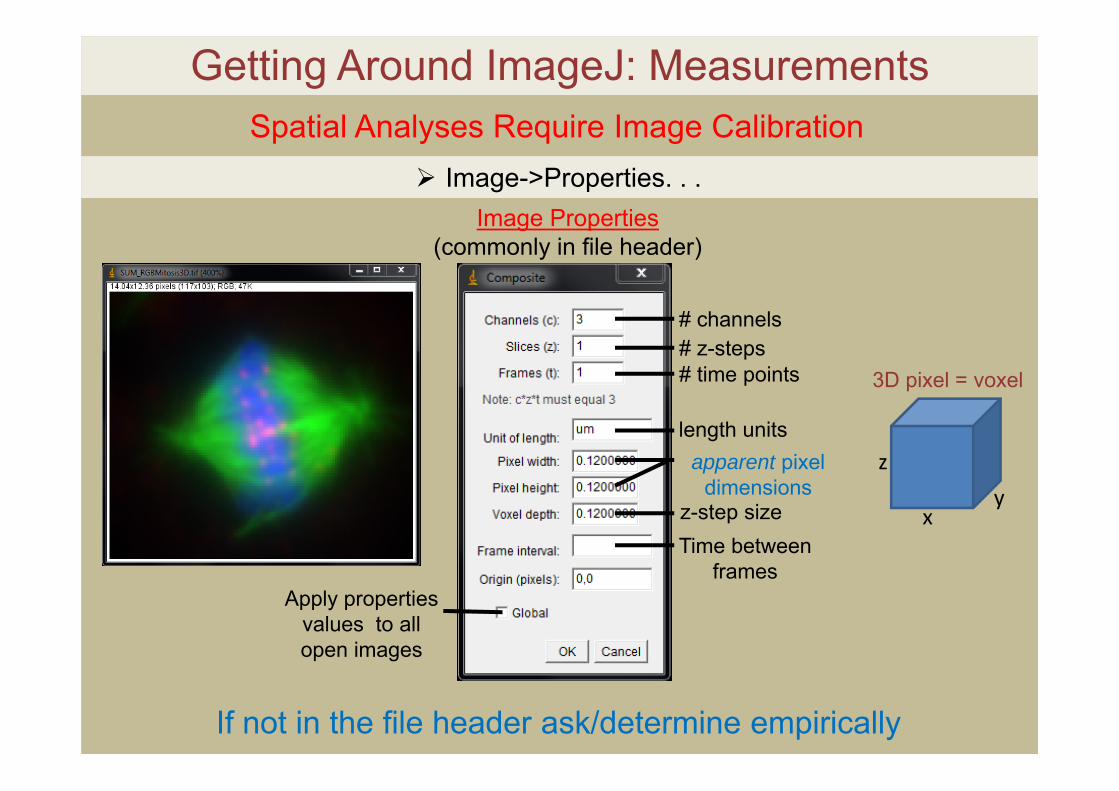
Getting Around ImageJ: MeasurementsSpatial Analyses Require Image Calibration
Image Properties (commonly in file header)
# channels# z-steps# time points
length unitsapparent pixel
dimensionsz-step sizeTime between
framesApply properties
values to all open images
Image->Properties. . .
If not in the file header ask/determine empirically
z
xy
3D pixel = voxel
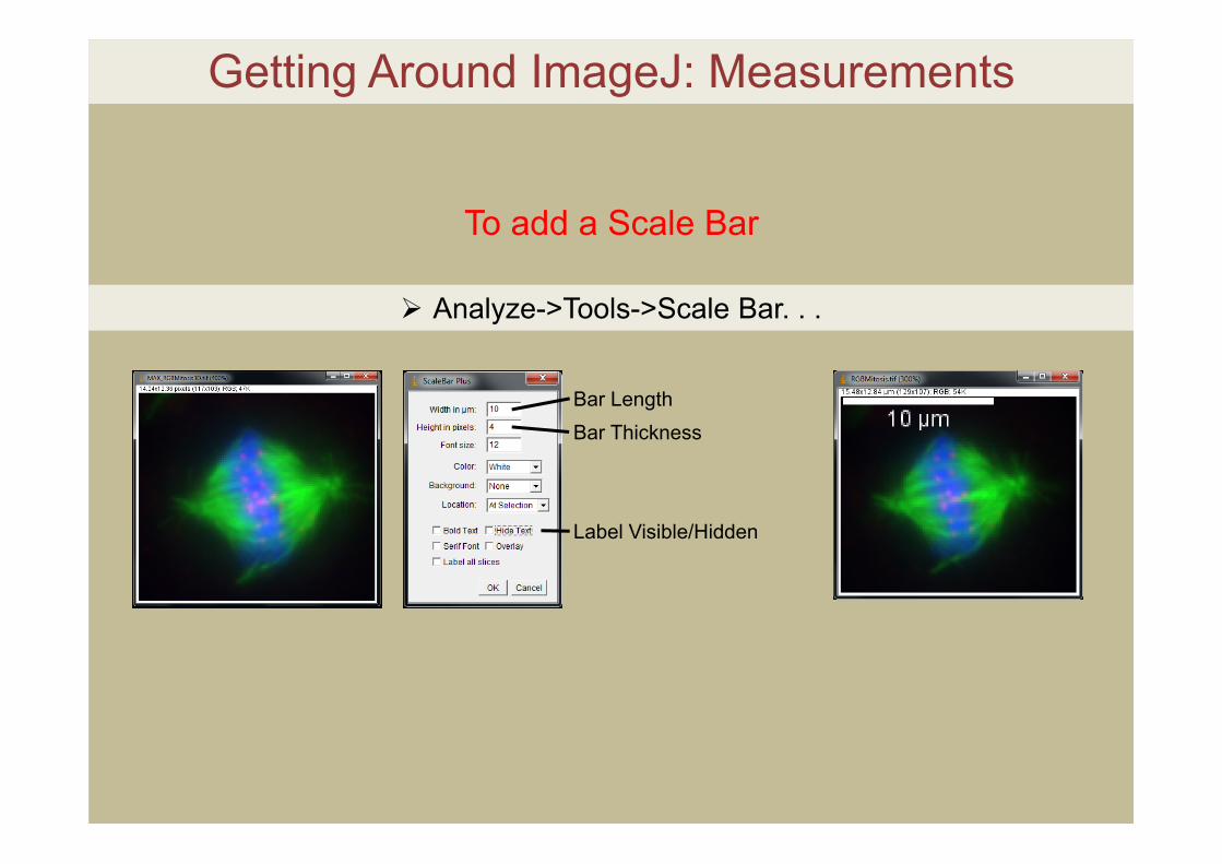
Getting Around ImageJ: Measurements
To add a Scale Bar
Analyze->Tools->Scale Bar. . .
Bar LengthBar Thickness
Label Visible/Hidden
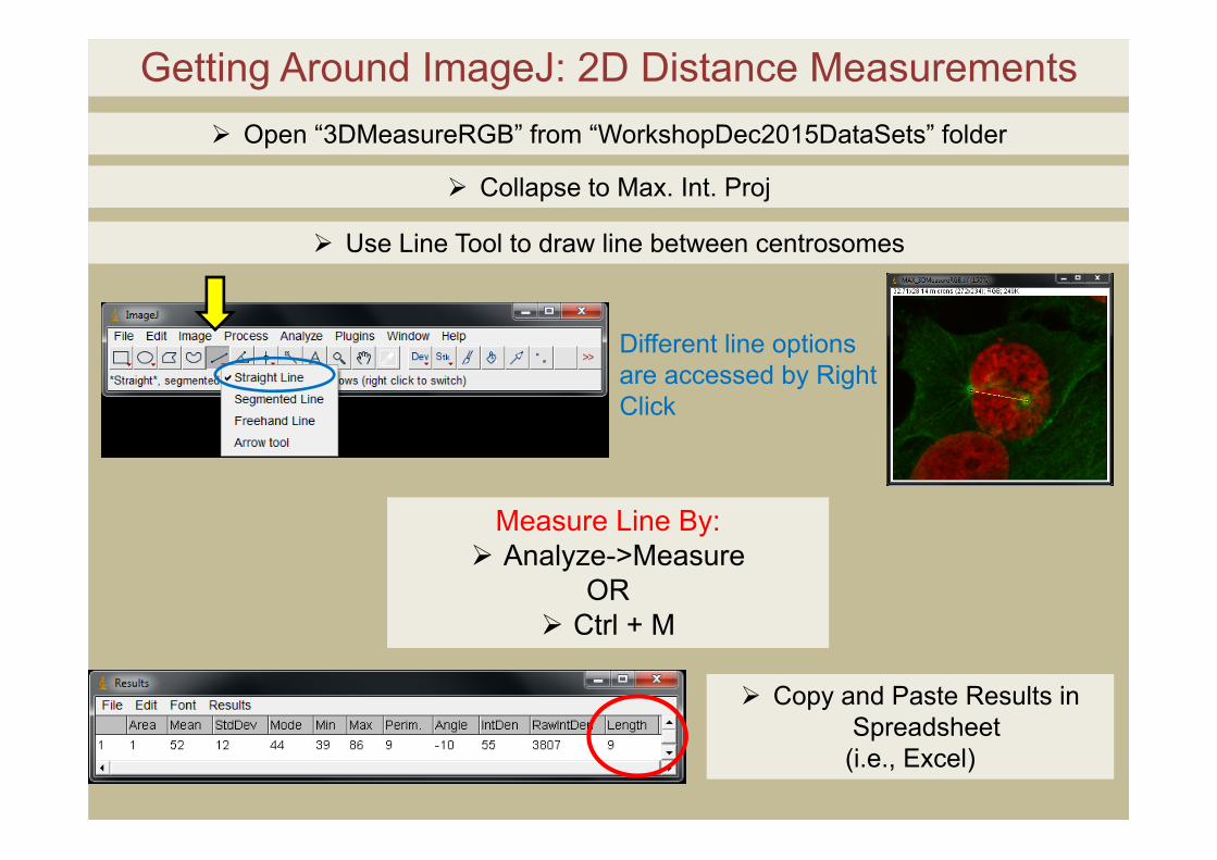
Getting Around ImageJ: 2D Distance Measurements
Copy and Paste Results in Spreadsheet
(i.e., Excel)
Open “3DMeasureRGB” from “WorkshopDec2015DataSets” folder
Collapse to Max. Int. Proj
Use Line Tool to draw line between centrosomes
Different line options are accessed by Right Click
Measure Line By: Analyze->Measure
OR Ctrl + M
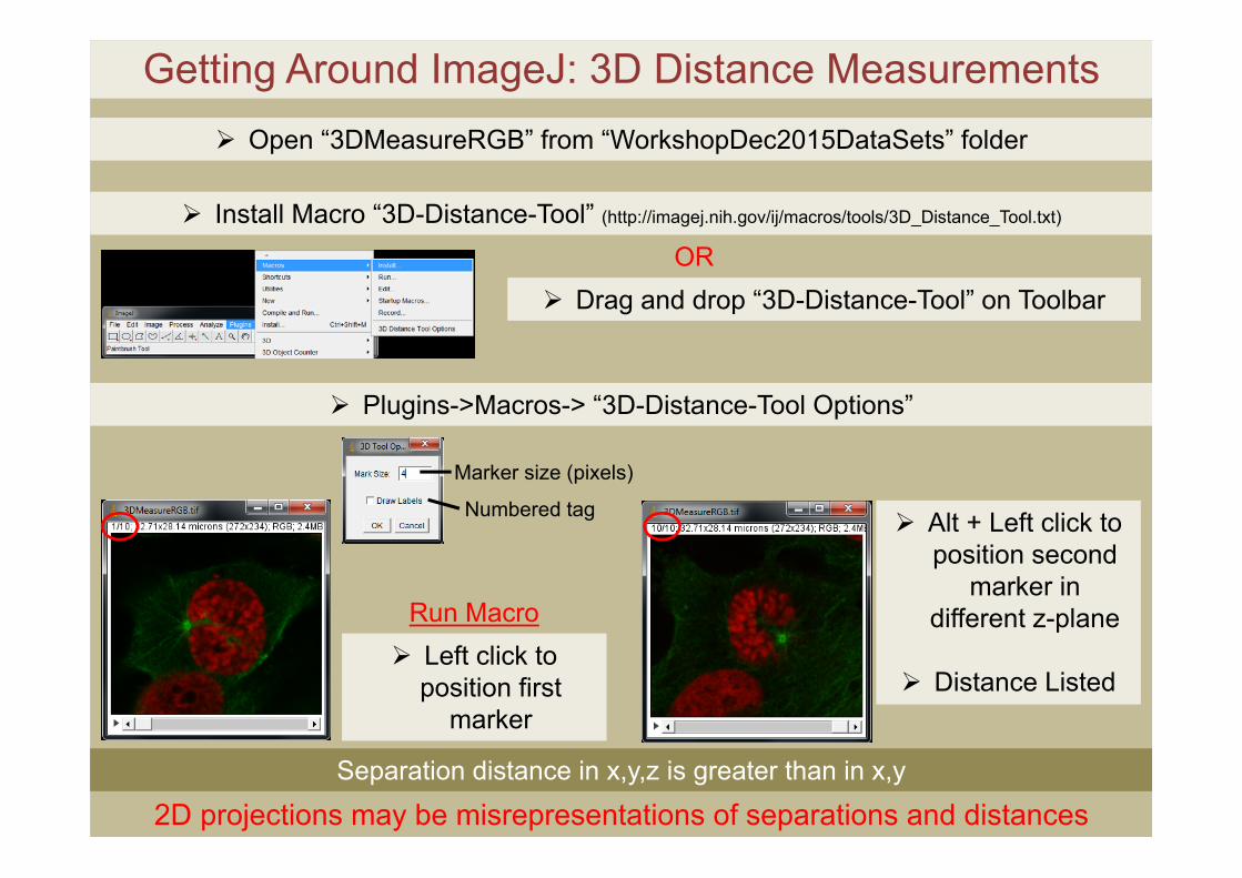
Getting Around ImageJ: 3D Distance Measurements
Install Macro “3D-Distance-Tool” (http://imagej.nih.gov/ij/macros/tools/3D_Distance_Tool.txt)
Drag and drop “3D-Distance-Tool” on ToolbarOR
Plugins->Macros-> “3D-Distance-Tool Options”
Left click to position first
marker
Alt + Left click to position second
marker in different z-plane
Distance Listed
Separation distance in x,y,z is greater than in x,y
2D projections may be misrepresentations of separations and distances
Open “3DMeasureRGB” from “WorkshopDec2015DataSets” folder
Run Macro
Marker size (pixels)
Numbered tag
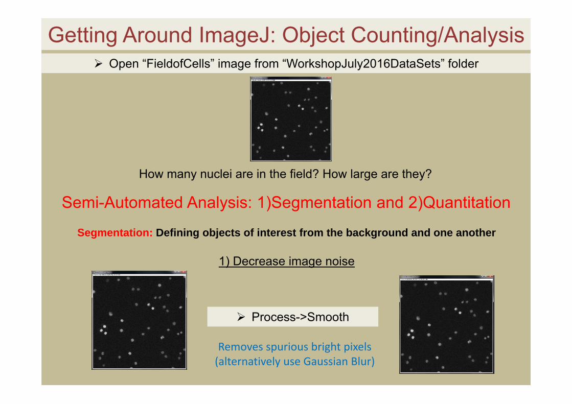
Getting Around ImageJ: Object Counting/Analysis Open “FieldofCells” image from “WorkshopJuly2016DataSets” folder
1) Decrease image noise
Process->Smooth
How many nuclei are in the field? How large are they?
Semi-Automated Analysis: 1)Segmentation and 2)Quantitation
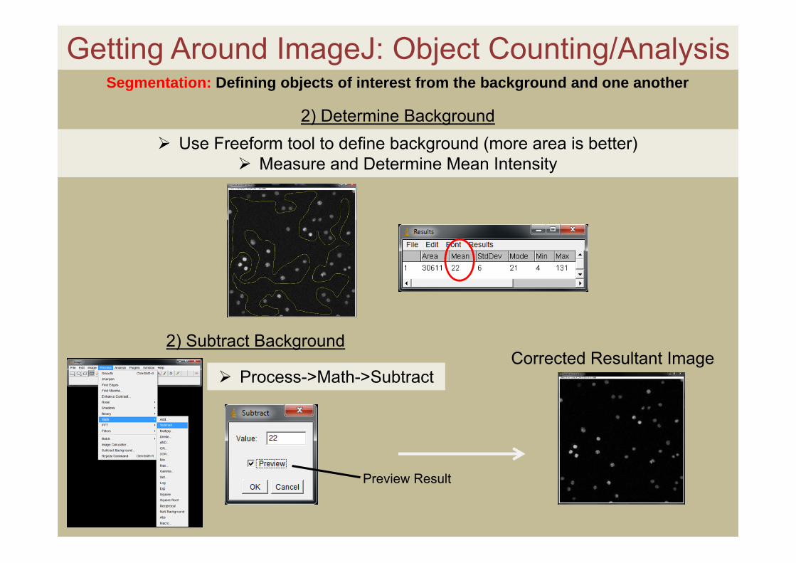
Segmentation: Defining objects of interest from the background and one another
Removes spurious bright pixels(alternatively use Gaussian Blur)
Getting Around ImageJ: Object Counting/Analysis
2) Subtract BackgroundCorrected Resultant Image
2) Determine Background Use Freeform tool to define background (more area is better)
Measure and Determine Mean Intensity
Process->Math->Subtract
Preview Result
Segmentation: Defining objects of interest from the background and one another
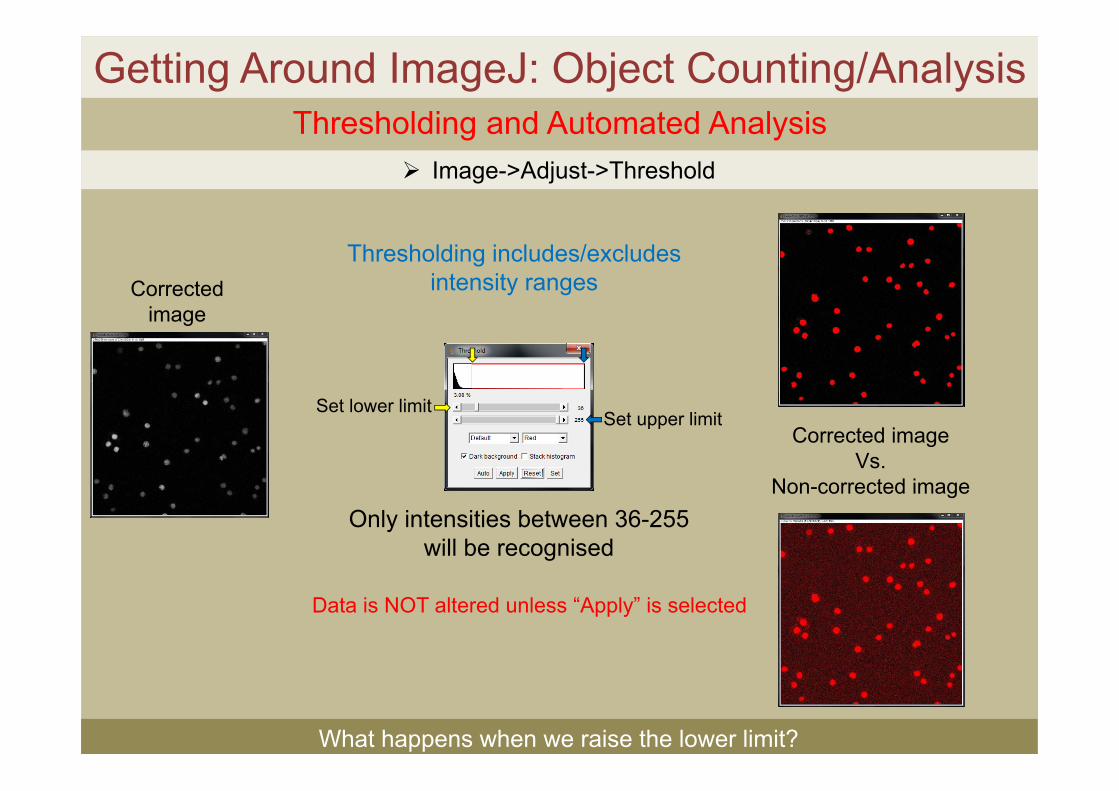
Getting Around ImageJ: Object Counting/Analysis Thresholding and Automated Analysis
Set upper limitSet lower limit
Corrected image
Image->Adjust->Threshold
Thresholding includes/excludes intensity ranges
Only intensities between 36-255 will be recognised
What happens when we raise the lower limit?
Corrected imageVs.
Non-corrected image
Data is NOT altered unless “Apply” is selected
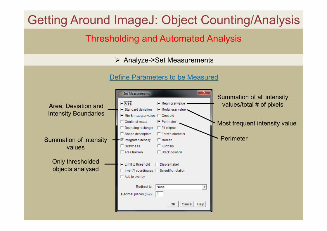
Getting Around ImageJ: Object Counting/Analysis
Define Parameters to be Measured
Summation of intensity values
Summation of all intensity values/total # of pixels
Most frequent intensity value
Only thresholdedobjects analysed
Analyze->Set Measurements
Area, Deviation and Intensity Boundaries
Perimeter
Thresholding and Automated Analysis
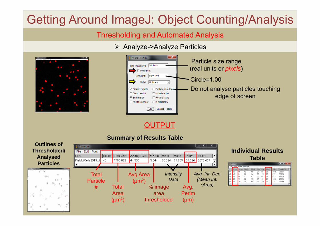
Getting Around ImageJ: Object Counting/Analysis Thresholding and Automated Analysis
Particle size range (real units or pixels)
Circle=1.00Do not analyse particles touching
edge of screen
Analyze->Analyze Particles
OUTPUT
Total Particle
# Total Area (m2)
Avg Area(m2)
% image area
thresholded
Intensity Data
Avg. Perim(m)
Avg. Int. Den(Mean Int.
*Area)
Summary of Results Table
Individual Results Table
Outlines of Thresholded/
Analysed Particles
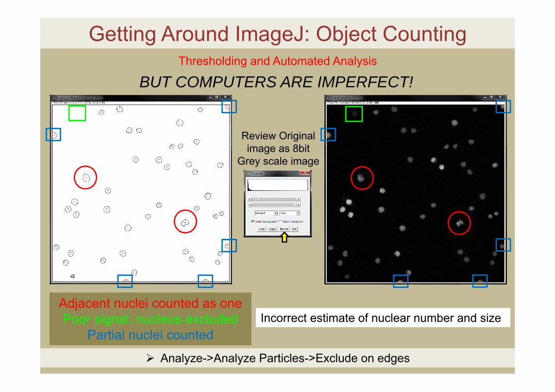
Getting Around ImageJ: Object Counting Thresholding and Automated Analysis
BUT COMPUTERS ARE IMPERFECT!
Adjacent nuclei counted as onePoor signal: nucleus excluded
Partial nuclei counted
Review Original image as 8bit
Grey scale image
Incorrect estimate of nuclear number and size
Analyze->Analyze Particles->Exclude on edges
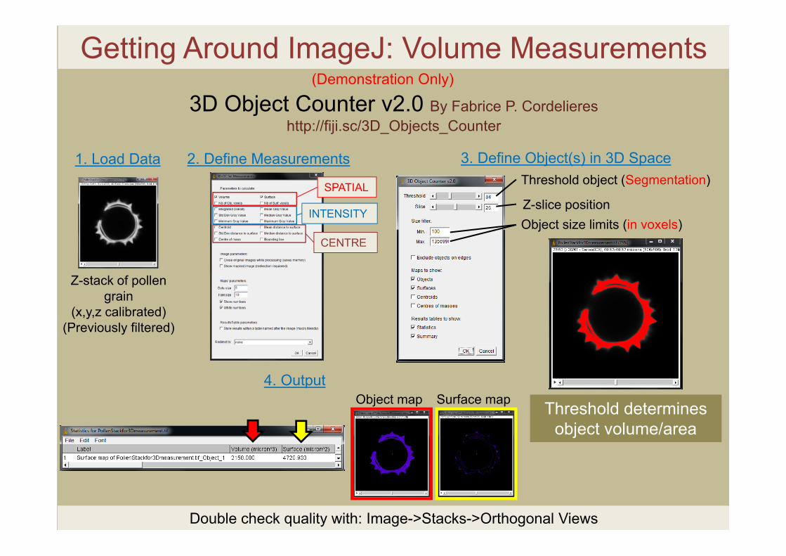
Getting Around ImageJ: Volume Measurements(Demonstration Only)
3D Object Counter v2.0 By Fabrice P. Cordeliereshttp://fiji.sc/3D_Objects_Counter
Threshold object (Segmentation)
Z-slice positionObject size limits (in voxels)
3. Define Object(s) in 3D Space
Z-stack of pollen grain
(x,y,z calibrated)(Previously filtered)
1. Load Data 2. Define Measurements
SPATIAL
INTENSITY
CENTRE
Threshold determines object volume/area
4. OutputObject map Surface map
Double check quality with: Image->Stacks->Orthogonal Views
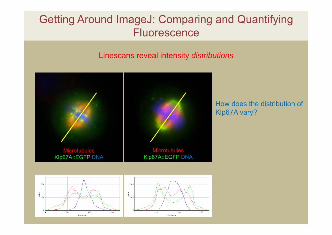
Getting Around ImageJ: Comparing and Quantifying Fluorescence
Linescans reveal intensity distributions
How does the distribution of Klp67A vary?
Microtubules Klp67A::EGFP DNA
Microtubules Klp67A::EGFP DNA
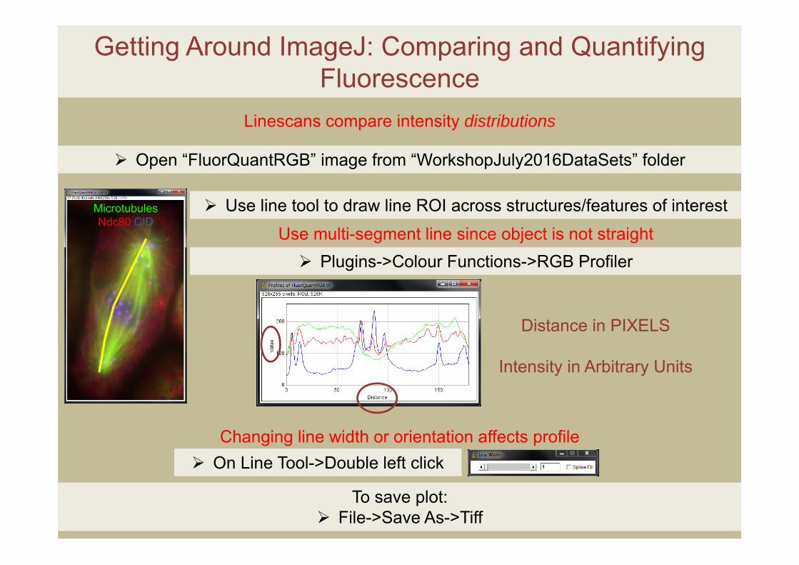
Getting Around ImageJ: Comparing and Quantifying Fluorescence
Linescans compare intensity distributions
Open “FluorQuantRGB” image from “WorkshopJuly2016DataSets” folder
Use line tool to draw line ROI across structures/features of interest
To save plot: File->Save As->Tiff
Use multi-segment line since object is not straight Plugins->Colour Functions->RGB Profiler
Distance in PIXELS
Intensity in Arbitrary Units
Changing line width or orientation affects profile On Line Tool->Double left click
MicrotubulesNdc80 CID
Getting Around ImageJ: Comparing and Quantifying Fluorescence
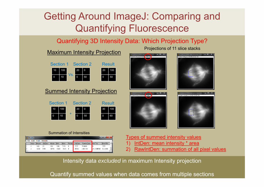
Quantifying 3D Intensity Data: Which Projection Type?
10 100
0 10
20 0
0 50
20 100
0 50
Section 1 Section 2 Result
10 100
0 10
20 0
0 50
30 100
0 60
Section 1 Section 2 Result
Vs.
+
Summed Intensity Projection
Maximum Intensity Projection
Intensity data excluded in maximum Intensity projection
Quantify summed values when data comes from multiple sections
Projections of 11 slice stacks
Summation of IntensitiesTypes of summed intensity values1) IntDen: mean intensity * area2) RawIntDen: summation of all pixel values
Getting Around ImageJ: Comparing and Quantifying Fluorescence
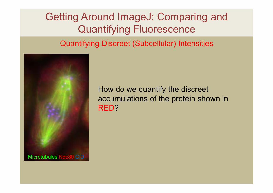
Quantifying Discreet (Subcellular) Intensities
How do we quantify the discreet accumulations of the protein shown in RED?
Microtubules Ndc80 CID
Getting Around ImageJ: Comparing and Quantifying Fluorescence
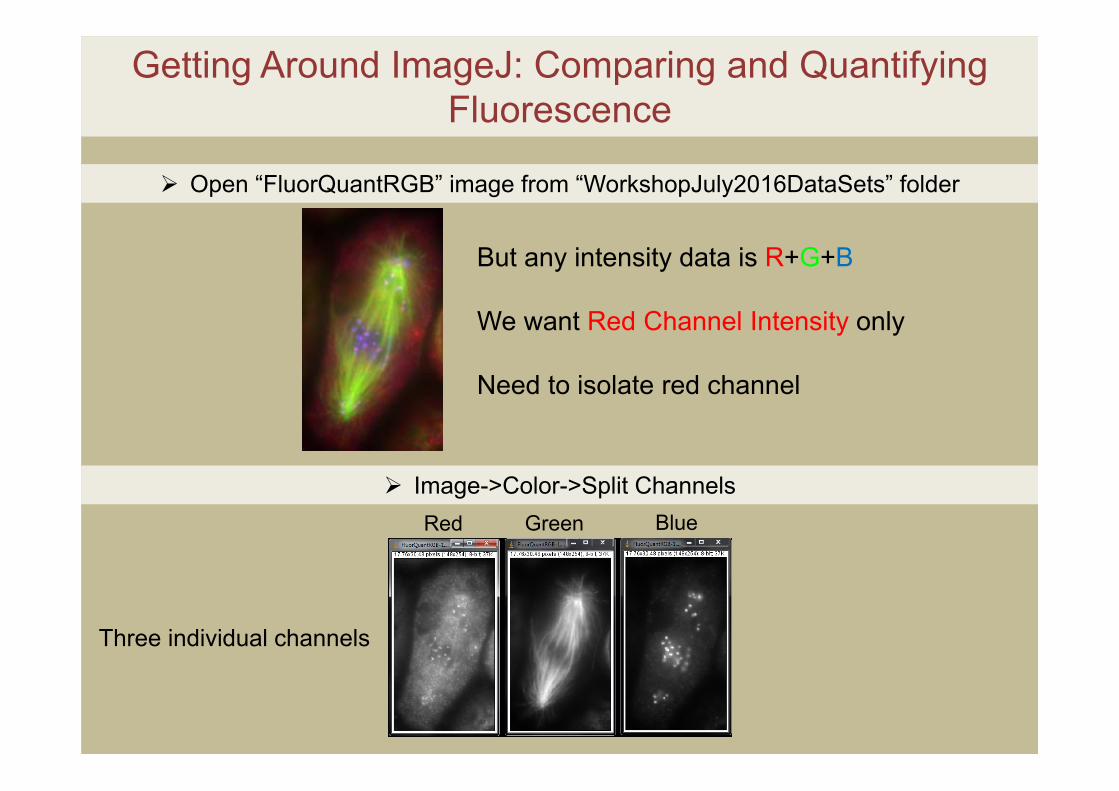
Open “FluorQuantRGB” image from “WorkshopJuly2016DataSets” folder
Image->Color->Split Channels
But any intensity data is R+G+B
We want Red Channel Intensity only
Need to isolate red channel
Red Green Blue
Three individual channels
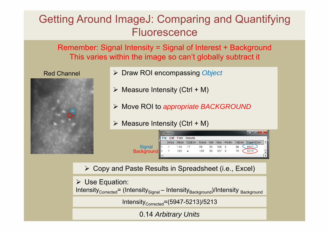
Getting Around ImageJ: Comparing and Quantifying Fluorescence
Draw ROI encompassing Object
Measure Intensity (Ctrl + M)
Move ROI to appropriate BACKGROUND
Measure Intensity (Ctrl + M)
Red Channel
SignalBackground
Use Equation:IntensityCorrected= (IntensitySignal – IntensityBackground)/Intensity Background
Remember: Signal Intensity = Signal of Interest + BackgroundThis varies within the image so can’t globally subtract it
IntensityCorrected=(5947-5213)/5213
Copy and Paste Results in Spreadsheet (i.e., Excel)
0.14 Arbitrary Units
Getting Around ImageJ: Comparing and Quantifying Fluorescence
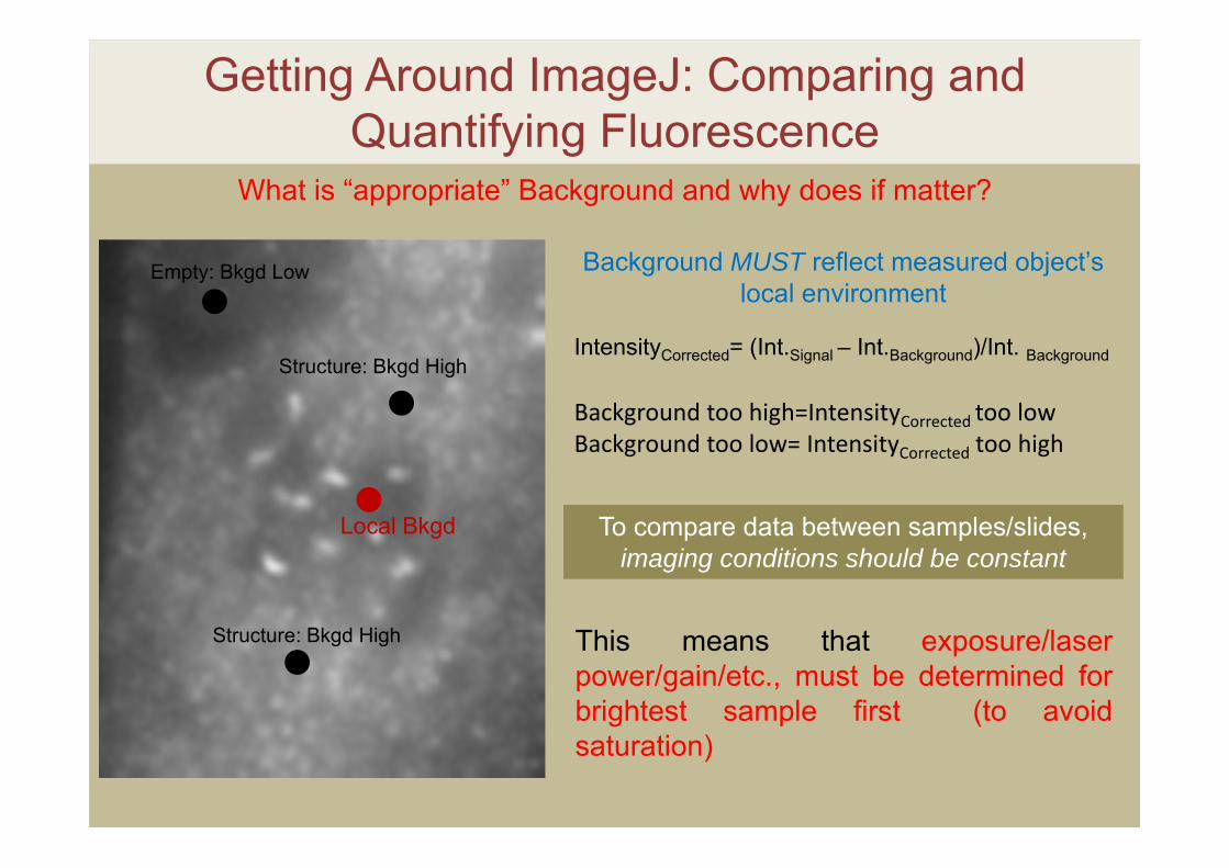
What is “appropriate” Background and why does if matter?
Structure: Bkgd High
Structure: Bkgd High
Empty: Bkgd Low
Local Bkgd
IntensityCorrected= (Int.Signal – Int.Background)/Int. Background
Background MUST reflect measured object’s local environment
Background too high=IntensityCorrected too lowBackground too low= IntensityCorrected too high
To compare data between samples/slides, imaging conditions should be constant
This means that exposure/laserpower/gain/etc., must be determined forbrightest sample first (to avoidsaturation)
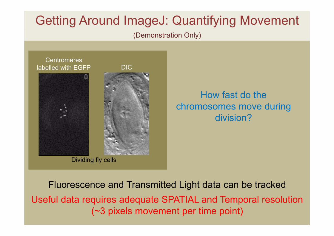
Getting Around ImageJ: Quantifying Movement
Useful data requires adequate SPATIAL and Temporal resolution(~3 pixels movement per time point)
Centromeres labelled with EGFP DIC
Dividing fly cells
Fluorescence and Transmitted Light data can be tracked
How fast do the chromosomes move during
division?
(Demonstration Only)
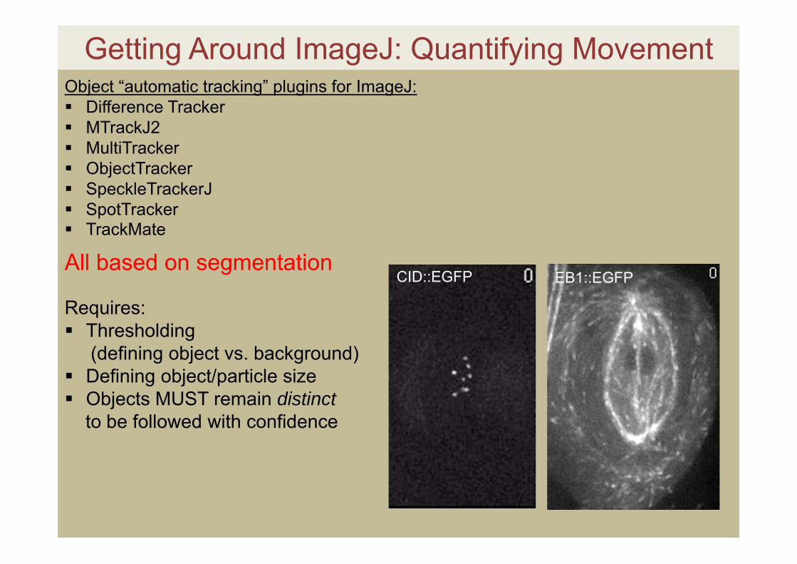
Getting Around ImageJ: Quantifying MovementObject “automatic tracking” plugins for ImageJ: Difference Tracker MTrackJ2 MultiTracker ObjectTracker SpeckleTrackerJ SpotTracker TrackMate
All based on segmentation
Requires: Thresholding
(defining object vs. background) Defining object/particle size Objects MUST remain distinct
to be followed with confidence
CID::EGFP EB1::EGFP
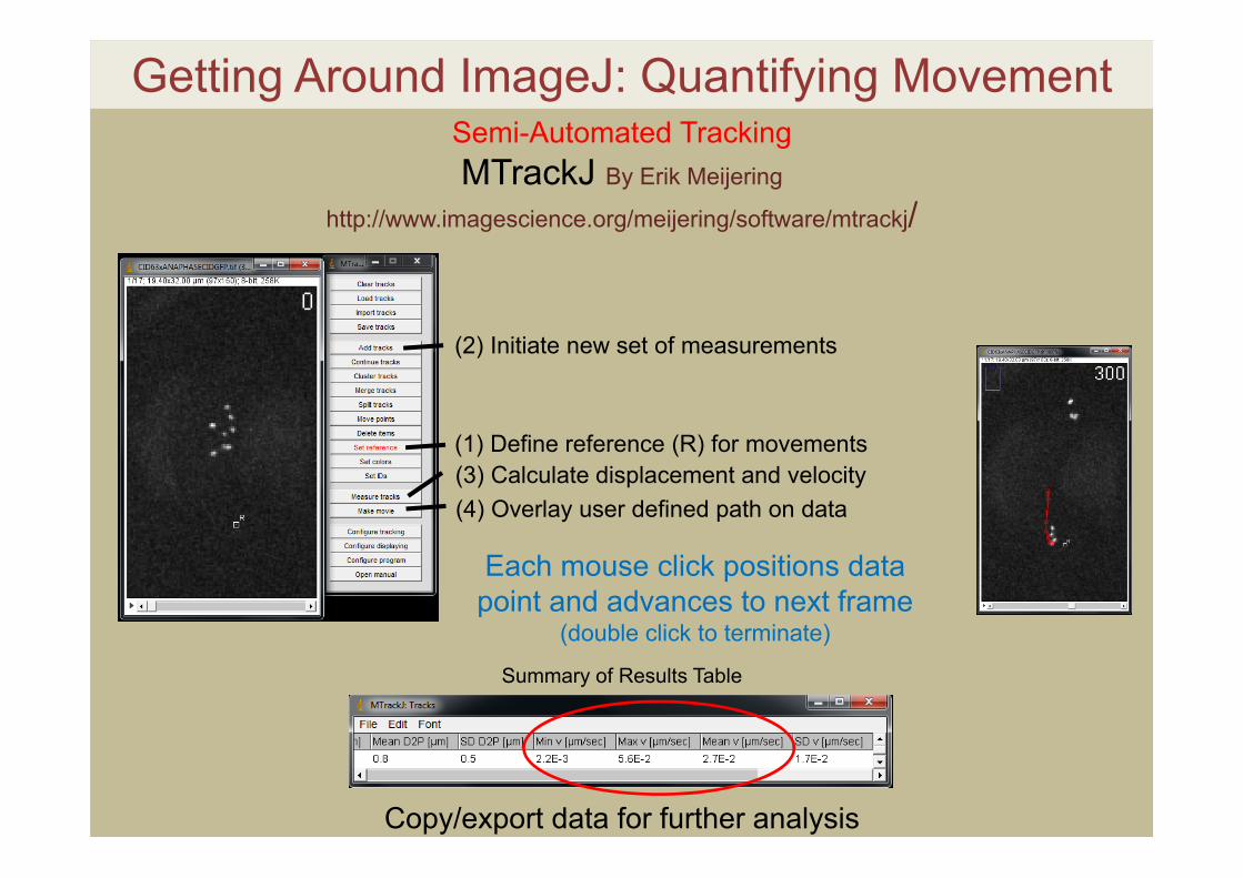
Getting Around ImageJ: Quantifying MovementSemi-Automated TrackingMTrackJ By Erik Meijering
http://www.imagescience.org/meijering/software/mtrackj/
Each mouse click positions data point and advances to next frame
(double click to terminate)
(1) Define reference (R) for movements
(2) Initiate new set of measurements
(3) Calculate displacement and velocity(4) Overlay user defined path on data
Copy/export data for further analysis
Summary of Results Table
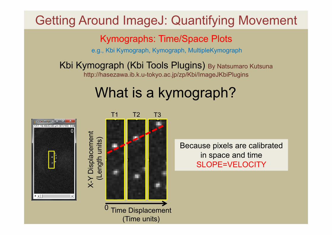
Getting Around ImageJ: Quantifying MovementKymographs: Time/Space Plots
e.g., Kbi Kymograph, Kymograph, MultipleKymograph
Kbi Kymograph (Kbi Tools Plugins) By Natsumaro Kutsunahttp://hasezawa.ib.k.u-tokyo.ac.jp/zp/Kbi/ImageJKbiPlugins
What is a kymograph?X
-Y D
ispl
acem
ent
(Len
gth
units
)
Time Displacement (Time units)
0
T1 T2 T3
Because pixels are calibrated in space and time
SLOPE=VELOCITY
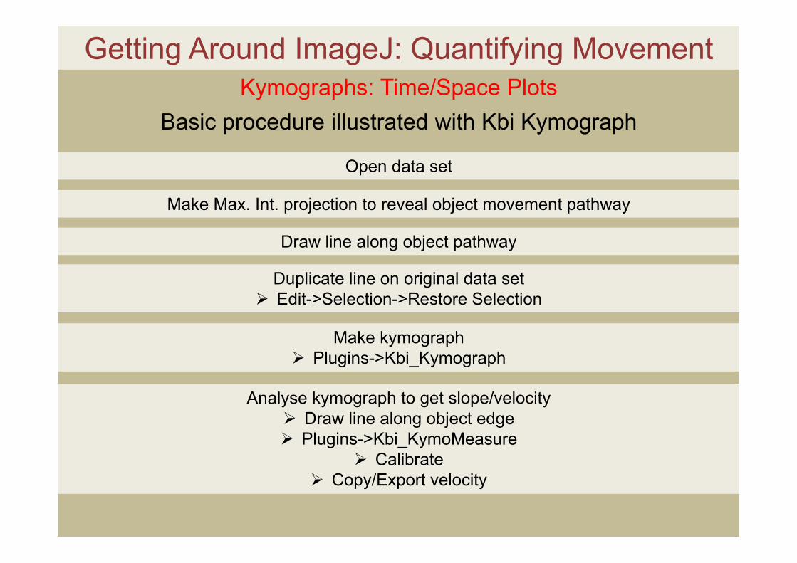
Getting Around ImageJ: Quantifying MovementKymographs: Time/Space Plots
Basic procedure illustrated with Kbi Kymograph
Open data set
Make Max. Int. projection to reveal object movement pathway
Draw line along object pathway
Duplicate line on original data set Edit->Selection->Restore Selection
Make kymograph Plugins->Kbi_Kymograph
Analyse kymograph to get slope/velocity Draw line along object edge Plugins->Kbi_KymoMeasure
Calibrate Copy/Export velocity
Questions?
http://micro.magnet.fsu.edu/primer/techniques/fluorescence/gallery/fleaslarge.html
https://royalsociety.org/collections/micrographia/

Thank you!
Jordan Taylor (TEM) [email protected]
Niki Murray (SEM) [email protected]
Remember, MMIC is free for Massey-affiliated Work!Please complete the feedback form
Top Related