


Languages
Pages
Legal

UIUC Physics 435 EM Fields & Sources I Fall Semester, 2007 Lecture Notes 7.5 Prof. Steven Errede
©Professor Steven Errede, Department of Physics, University of Illinois at Urbana-Champaign, Illinois 2005 - 2008. All rights reserved.
1
LECTURE NOTES 7.5
Laplace’s Equation in Rectangular/Cartesian Coordinates
Griffiths Example 3.3: Two infinite, grounded metal plates lie parallel to the x-z plane, one located at y = 0 and the other located at y = a. The back side (at x = 0) is closed off with an infinite metal strip insulated from the two parallel planes, and maintained at a potential V(0,y,z) = V0. z 3 ( ) 00, , constant potentialV y z V= = y a= 1 Ο y V(x,0, z) = 0 0y = x 2 ( ), , 0V x a z = Find the potential ( ), ,V x y z inside the “slot” region.
⇒ First, recognize that because ( ), ,V x y z has no explicit z-dependence, this problem is actually only a 2-dimensional problem! Top View of Problem: 3 ( ) 00,V y V= 0y = y a=
ˆ outof pagez⎛ ⎞
⎜ ⎟⎝ ⎠
z y
1 2 ( ),0 0V x = ( ), 0V x a =
x Find ( ),V x y in “slot” ⇐ independent of z for any value of z.
Because of this fact: ( ) ( ) ( ) ( )2 22 2
2 2
, ,, , , 0
V x y V x yV x y z V x y
x y∂ ∂
∇ ⇒ ∇ = + =∂ ∂
UIUC Physics 435 EM Fields & Sources I Fall Semester, 2007 Lecture Notes 7.5 Prof. Steven Errede
©Professor Steven Errede, Department of Physics, University of Illinois at Urbana-Champaign, Illinois 2005 - 2008. All rights reserved.
2
Boundary Conditions: 1.) ( ), 0 0V x y = =
2.) ( ), 0V x y a= =
3.) ( ) 00,V x y V= = (constant potential)
4.) ( ) ( ), 0 i.e. , 0V x y V x y→∞ → = ∞ = Try product solution of form: ( ) ( ) ( ),V x y X x Y y=
( ) ( )2 2
2 2
, ,0
V x y V x yx y
∂ ∂+ =
∂ ∂
( ) ( )( ) ( ) ( )( )2 2
2 2 0X x Y x X x Y y
x y∂ ∂
= + =∂ ∂
( ) ( ) ( ) ( ) ( ) ( )2 2
2 2 0 now divide both sides by X x Y y
Y y X x X x Y yx y
∂ ∂= + = ⇐
∂ ∂
( )( )
( )( )2 2
2 2
function of x only function of y only
1 1 0X x Y y
X x x Y y y∂ ∂
+ =∂ ∂
∴ must equal ∴ must equal a constant, e.g. a constant, e.g. = C1 = C2 Thus: 1 2 0C C+ = or 1 2.C C= −
Then: ( )
( )( )
( )2 2
1 22 2
1 1 and d X x d Y y
C CX x dx Y y dy
= = (n.b. have total derivatives now!)
Or: ( ) ( ) ( ) ( )2 2
1 22 2 d X x d Y y
C X x C Y ydx dy
= =
Or: ( ) ( ) ( ) ( )2 2
1 22 2=0 0d X x d Y y
C X x C Y ydx dy
− − =
but 1 2C C= −
( ) ( ) ( ) ( )2 2
1 12 2 0 0d X x d Y y
C X x C Y ydx dy
∴ − = + =
Let 21 0 :C k= >
( )( )
want exponential solutions for
want sine/cosine solutions for
X x
Y y
⎛ ⎞⎜ ⎟⎜ ⎟⎝ ⎠
Thus, we have:
( ) ( )2
22 0
d X xk X x
dx− = and ( ) ( )
22
2 0d Y y
k Y ydy
+ =
UIUC Physics 435 EM Fields & Sources I Fall Semester, 2007 Lecture Notes 7.5 Prof. Steven Errede
©Professor Steven Errede, Department of Physics, University of Illinois at Urbana-Champaign, Illinois 2005 - 2008. All rights reserved.
3
General Solutions for X(x) and Y(y): Because we (deliberately) chose 2
1 0,C k= > then general solutions for X(x) and Y(y) are of the form: X(x) = Aekx + Be−kx and Y(y) = C sin(ky) + D cos(ky) ⇐ EXPLICITLY put these back in above diff eqn’s and verify that these are correct!! n.b. we deliberately chose 2
1 0C k= > because of the boundary conditions: 1) ( , 0) 0 V x y = = 2) ( , ) 0 V x y a= = 3) 0( 0, ) V x y V= = 4) ( , ) 0V x y= ∞ = ⇐ Cannot be sine or cosine solutions for x! Then: ( ) ( ) ( ), ( ) ( ) sin coskx kxV x y X x Y y Ae Be C ky D ky−⎡ ⎤= = + +⎡ ⎤⎣ ⎦⎣ ⎦ Now impose boundary conditions: BC 4 : ( ), 0 V x y= ∞ = ⇒ A = 0 ( ) ( ) ( ) , sin coskxV x y Be C ky D y−∴ = +⎡ ⎤⎣ ⎦ Absorb constant B into C and D: ( ) ( ) ( ), sin coskxV x y e C ky D y−= +⎡ ⎤⎣ ⎦ Impose BC 1 and 2 : ( ) ( ), 0 0 and , 0 V x y V x y a= = = = ⇒ D = 0
( ) ( ) , sinkxV x y Ce ky−∴ = automatically satisfies ( ),0 0V x = ( ) ( ), sin 0kxV x y e ka−= = requires .ka nπ= Then ( )sin 0nπ = where 1,2,3,n = …
∴ Define: , 1, 2,3nnk naπ
= = …
General specific solution to Laplace’s equation (for this problem):
( ) ( )1
, sinnk xn n
nV x y C e k y
∞−
=
=∑ where , 1, 2,3,nnk naπ
= = ……
Note that:
( ) ( ) ( ) ( )2
1 1, , sin satisfies , 0nk x
n n nn n
V x y V x y C e k y V x y∞ ∞
−
= =
= = ∇ =∑ ∑ (and all 4 BC’s) by superposition
principle, since ( ) ( ), sinnk xn n nV x y C e k y−= individually satisfy ( )2 , 0V x y∇ = and all 4 BC’s for
each/every value of n = 1,2,3,…. Impose final (remaining) BC: 3 ( ) 00, constantV y V= =
( ) ( )00
10, sin constantn n
nV y C e k y V
∞
=
= = =∑
V(x,y) must be periodic in y. ⇒ sine and/or cosine type solutions (not exponentials or sinh/ cosh solutions).

UIUC Physics 435 EM Fields & Sources I Fall Semester, 2007 Lecture Notes 7.5 Prof. Steven Errede
©Professor Steven Errede, Department of Physics, University of Illinois at Urbana-Champaign, Illinois 2005 - 2008. All rights reserved.
4
( ) ( ) 01
Fourier Series!!
0, sin constantn nn
V y C k y V∞
=
= = =∑
To determine the ,s
nC′ multiply both sides of above equation by e.g. sin(kmy) and integrate over y from y = 0 to y = a. i.e. take inner product!
( ) ( ) ( ) ( ) ( )01
0, sin sin sin sinm n n m mn
V y k y C k y k y V k y∞
=
= =∑
( ) ( ) ( ) ( ) ( )
( ) ( ) ( )( )
00 0 01
00 01
11 cos, 2
1i.e. = 0 for 1 cos for 2 2
0, sin sin sin sin
sin sin sin
am onm n
mn
mnm
a a a
m n n m mn
a a
n n m mn
n n k yk kk an m ka a kn m
V y k y dy C k y k y dy V k y dy
C k y k y dy V k y dy
π πδ
δ
∞
=
∞
=−⎛ ⎞ == =⎜ ⎟
⎝ ⎠≠⎛ ⎞ = −
⎜ ⎟= = =⎜ ⎟⎝ ⎠
= =
= =
∑∫ ∫ ∫
∑ ∫ ∫
( )( )
( )( )1 cos
m
m
a
a mm
mka
ππ
π= −
=
( )( )0 1 cos2 n nma aC V n
mδ π
π∴ = − or: ( )( )0
2 1 cosnC V nn
ππ
= −
0 for
for 2
nm n ma m n
δ = ≠⎛ ⎞⎜ ⎟⎜ ⎟= =⎜ ⎟⎝ ⎠
piece-wise continuous function:
Now ( )1 cos 0nπ− = if n = even (2, 4, 6,. . . .) +V0 = 2 if n = odd (1, 3, 5,. . . .)
∴ 04 odd integers onlynC V n
nπ= = −a 0 +a y
−V0 Odd function on interval a y a− ≤ ≤ ⇒only odd n terms!!
04
nC Vnπ
= n = odd #’s = 1, 3, 5, . . . .
∴ Final, fully-specified for ( ),V x y is:
( ) ( )0
#
4 1, sinnk xn
n odd s
VV x y e k ynπ
∞−
=
⎛ ⎞= ⎜ ⎟⎝ ⎠
∑ where: ( ) 1,3,5,. . . . odd integersnnk naπ
= =
( ) ( )0
#
4 1, sinn x a
n odd s
VV x y e n y an
π ππ
∞−
=
⎛ ⎞= ⎜ ⎟⎝ ⎠
∑
All even Cn = 0
= Fourier Coefficients Cn for Bipolar Square Wave!!!
UIUC Physics 435 EM Fields & Sources I Fall Semester, 2007 Lecture Notes 7.5 Prof. Steven Errede
©Professor Steven Errede, Department of Physics, University of Illinois at Urbana-Champaign, Illinois 2005 - 2008. All rights reserved.
5
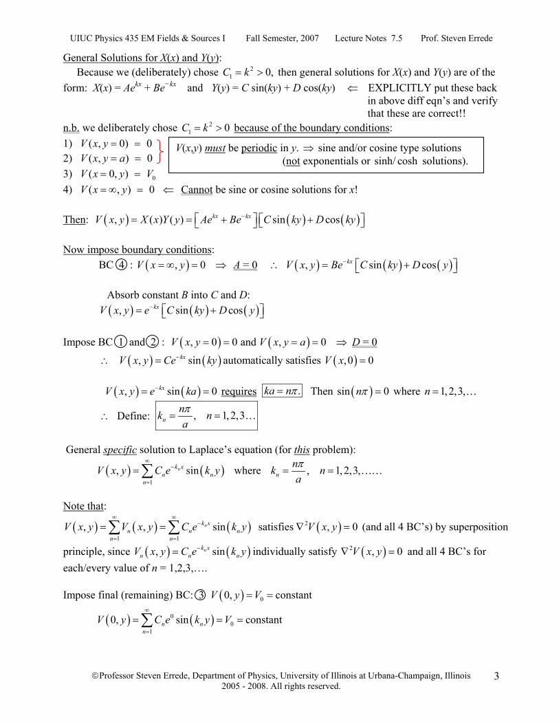
Let 2 1n = + then:
( ) ( )( ) ( )2 10
0
4 1 2 1, sin2 1
x aV yV x y e aπ π
π
∞− +
=
+⎛ ⎞⎛ ⎞= ⎜ ⎟ ⎜ ⎟+⎝ ⎠ ⎝ ⎠∑
n.b. This ∞ -series actually has an analytic representation!!!
( ) ( )10 sin2, tansin
y aVV x yxa
ππ π
− ⎡ ⎤⎛ ⎞= ⎢ ⎥⎜ ⎟⎝ ⎠ ⎣ ⎦
UIUC Physics 435 EM Fields & Sources I Fall Semester, 2007 Lecture Notes 7.5 Prof. Steven Errede
©Professor Steven Errede, Department of Physics, University of Illinois at Urbana-Champaign, Illinois 2005 - 2008. All rights reserved.
6
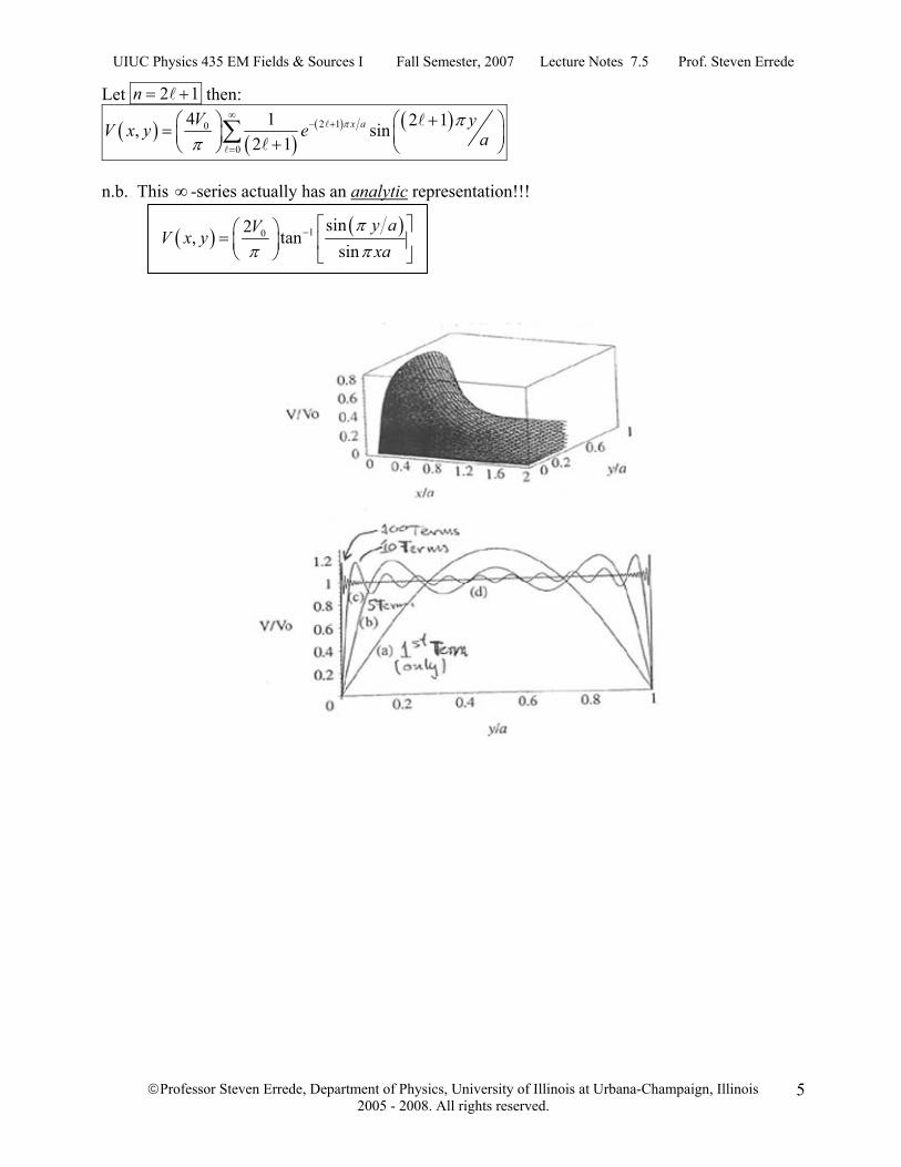
Griffiths Example 3.4 Two infinitely long, grounded metal plates lie parallel to the x – z plane, one at y = 0 and the other at y = a. Two additional infinitely long metal strips lie parallel to the y – z plane, one at x = −b and the other at x = +b, which are insulated from the first two grounded metal plates and maintained at a constant potential of ( ) 0, ,V x b y z V= ± = . Find the potential ( ), ,V x y z inside the resulting rectangular metal pipe:
First, recognize (again) that ( ), ,V x y z inside the
infinitely long in ˆ direction
rectangular pipez
has no explicit z-dependence. ⇒ (again) this problem is actually a 2 dimensional problem!!! Top View:
Note also that (again) this problem has translational invariance in z, i.e. ( ), ,V x y z does NOT depend on z.
Laplace’s Equation ( )2 , , 0V x y z∇ = in Rectangular/Cartesian Coordinates
UIUC Physics 435 EM Fields & Sources I Fall Semester, 2007 Lecture Notes 7.5 Prof. Steven Errede
©Professor Steven Errede, Department of Physics, University of Illinois at Urbana-Champaign, Illinois 2005 - 2008. All rights reserved.
7
Find ( ),V x y inside the rectangular pipe, satisfying Laplace’s Equation
( ) ( ) ( )2 22
2 2
, ,, 0 0
V x y V x yV x y
x y∂ ∂
∇ = ⇒ + =∂ ∂
in Cartesian/rectangular coordinates
subject to the boundary conditions: 1) ( ), 0 0V x y = = 2) ( ), 0V x y a= =
3) ( ) 0,V x b y V= − = 4) ( ) 0,V x b y V= = Again, try a product solution of form: ( ) ( ) ( ),V x y X x Y y= Get:
( ) ( )2
12 0d X x
C X xdx
− = ( ) ( )2
22 0d Y y
C Y ydy
− =
with: C1 + C2 = 0 i.e. C2 = − C1 Let: 2
1
0n.b. we deliberately chose this because we will needsine/cosine type solutionsin portion (i.e. for ( ))
C k
y- Y y
= > 22 1 C C k⇒ = − = −
to satisfy the periodic boundary conditions: 1) V(x,y=0) = 0 and 2) V(x,y=a) = 0 i.e. Y(y=0) = 0 i.e. Y(y=a) = 0 only sin (ky) can do this. Then:
( ) ( )2
22 0
d X xk X x
dx− = ( ) ( )
22
2 0d Y y
k Y ydy
+ =
General solutions for X(x) + Y(y) are (again) of the form: X(x) = Aekx + Be−kx and Y(y) = C sin (ky) + D cos (ky) Then: V(x,y) = X(x)Y(y) = [Aekx + Be−kx] [C sin(ky) + D cos(ky)] However, note that specify linear orthogonal combinations of ekx ± e−kx
give: ( )
( )
1sinh( )21cosh( )2
kx kx
kx kx
kx e e
kx e e
−
−
⎧ ⎫= −⎪ ⎪⎪ ⎪⎨ ⎬⎪ ⎪= +⎪ ⎪⎩ ⎭
or: ( ) ( )( )
( ) ( )( )
1 cosh sinh21 cosh sinh2
kx
kx
e kx kx
e kx kx−
⎧ ⎫= +⎪ ⎪⎪ ⎪⎨ ⎬⎪ ⎪= −⎪ ⎪⎩ ⎭

UIUC Physics 435 EM Fields & Sources I Fall Semester, 2007 Lecture Notes 7.5 Prof. Steven Errede
©Professor Steven Errede, Department of Physics, University of Illinois at Urbana-Champaign, Illinois 2005 - 2008. All rights reserved.
8
• We could have instead, alternatively/equivalently chosen X(x) = [ ]cosh( ) sinh( )A kx B kx′ ′+ • Now because x = ∞ is excluded in this problem we cannot apriori reject the Aekx term in the
X(x) = [Aekx + Be−kx] form of the X(x) solution • Both of the terms Aekx + Be−kx must be allowed here because of this. • If we look at the X(x) = [[ ]cosh( ) sinh( )A kx B kx′ ′+ version of the X(x) solution, we see that
BC 3 : V(x = −b,y) = V0 and BC 4 : V(x=+b,y) = V0 means that V(x,y) = V(−x,y) is an even function of x with respect to .x x→ −
Now: ( ) ( )cosh coshx x− = + even fcn(x)
( )sinh sinh( )x x− = − odd fcn(x) ∴ 0B′ = , or equivalently, A = +B i.e., Aekx + Be−kx = Aekx + Ae−kx = A(ekx + e−kx) = 2A(cosh(kx) Thus 2A A′ = . Then:
[ ]( , ) ( ) ( ) cosh( ) sin( ) cos( )V x y X x Y y A kx C ky D ky= = + absorb constant A into C & D: ( ) ( ) ( ), cosh( )[ sin( ) cos( )]V x y X x Y y kx C ky D ky= = +
Now impose boundary conditions 1 and 2 : 1 V(x,y=0) = 0 2 V(x, y=a) = 0 i.e. ( 0) 0Y y = = i.e. ( ) 0Y y a= =
⇒ D must = 0 sin( ) sin( ) 0ka nπ⇒ = = i.e. , 1, 2,3,ka n nπ= = …
i.e. nnkaπ⎛ ⎞= ⎜ ⎟
⎝ ⎠, 1, 2,3,n = …
Then:
( ) ( ) ( ), cosh sin with , 1, 2,3,n n n n nnV x y C k x k y k naπ⎛ ⎞= = =⎜ ⎟
⎝ ⎠…
Thus: ( ) ( ) ( ) ( )1 1
, , cosh sinn n n nn n
V x y V x y C k x k y∞ ∞
= =
= =∑ ∑ ⇐
General Specific Solution to Laplace’s equation for this problem.
UIUC Physics 435 EM Fields & Sources I Fall Semester, 2007 Lecture Notes 7.5 Prof. Steven Errede
©Professor Steven Errede, Department of Physics, University of Illinois at Urbana-Champaign, Illinois 2005 - 2008. All rights reserved.
9
This ( ),V x y satisfies ( )2 , 0V x y∇ = with , 1, 2,3,nnk naπ⎛ ⎞= =⎜ ⎟
⎝ ⎠… . and all four BC’s.
Now, from BC’s 3 and 4 , namely that: ( ) 0,V x b y V= ± = Noting that: cosh( ) cosh( )n nk b k b= −
Then: ( ) ( ) 01
, cosh sin( )n n nn
V x b y C k b k y V∞
=
= ± = =∑ with , 1, 2,3,...nnk naπ⎛ ⎞= =⎜ ⎟
⎝ ⎠
Now multiply both sides of this relation by sin (kmy) and integrate along y from y = 0 to y = a to project out (i.e. take inner product) in order to determine the coefficients nC :
( )( )
( )( )
( ) ( ) ( )0 0 01
1 1cos2
1 cos2
sin cosh sin sin
am o nm
m n
nm
a a
m n n n mn
nk yk ka am
m
V k y d y C k b k y k y dy
π δ
π δπ
∞
=⎛ ⎞=− = ⎜ ⎟⎝ ⎠
= − =
= ∑∫ ∫
( ) ( )0 1 cos( ) cosh2 n n nm
a aV m C k bm
π δπ
∴ − = 0 if
1 if nm m n
m nδ = ≠⎛ ⎞⎜ ⎟= =⎝ ⎠
( )( )0
1 cos2 coshn
n
nC V
n k bπ
π⎡ ⎤−⎛ ⎞∴ = ⎢ ⎥⎜ ⎟
⎝ ⎠ ⎣ ⎦ , 1, 2,3,n
nk naπ⎛ ⎞= =⎜ ⎟
⎝ ⎠…
n.b. odd n integers only!! (all even n integers have 0nC = ) because ( )0 for even
1 cos2 for odd
nn
nπ
⎛ ⎞− =⎡ ⎤ ⎜ ⎟⎣ ⎦
⎝ ⎠
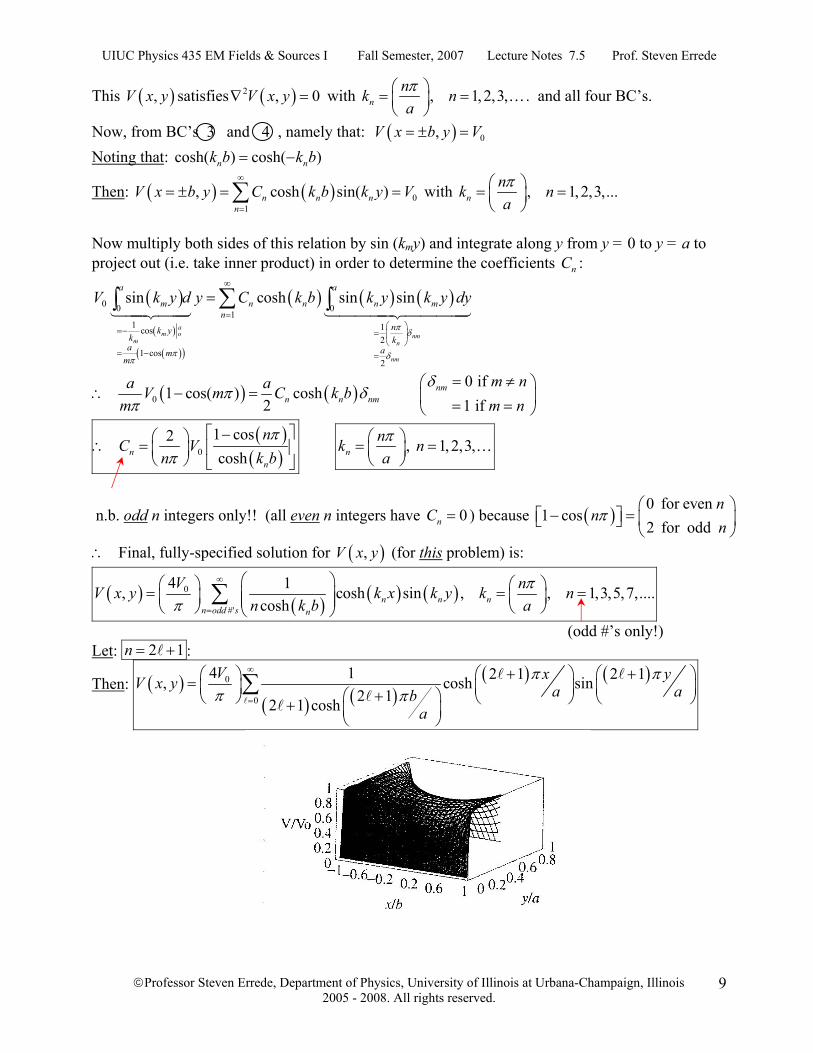
∴ Final, fully-specified solution for ( ),V x y (for this problem) is:
( ) ( ) ( ) ( )0
#'
4 1, cosh sin , , 1,3,5,7,....cosh n n n
n odd s n
V nV x y k x k y k nn k b a
ππ
∞
=
⎛ ⎞⎛ ⎞ ⎛ ⎞= = =⎜ ⎟ ⎜ ⎟⎜ ⎟ ⎜ ⎟ ⎝ ⎠⎝ ⎠ ⎝ ⎠∑
(odd #’s only!) Let: 2 1n = + :
Then: ( )( ) ( )
( ) ( )0
0
4 1 2 1 2 1, cosh sin2 12 1 cosh
V x yV x y a aba
π ππ π
∞
=
+ +⎛ ⎞ ⎛ ⎞⎛ ⎞= ⎜ ⎟ ⎜ ⎟ ⎜ ⎟+⎛ ⎞⎝ ⎠ ⎝ ⎠ ⎝ ⎠+ ⎜ ⎟⎝ ⎠
∑
UIUC Physics 435 EM Fields & Sources I Fall Semester, 2007 Lecture Notes 7.5 Prof. Steven Errede
©Professor Steven Errede, Department of Physics, University of Illinois at Urbana-Champaign, Illinois 2005 - 2008. All rights reserved.
10
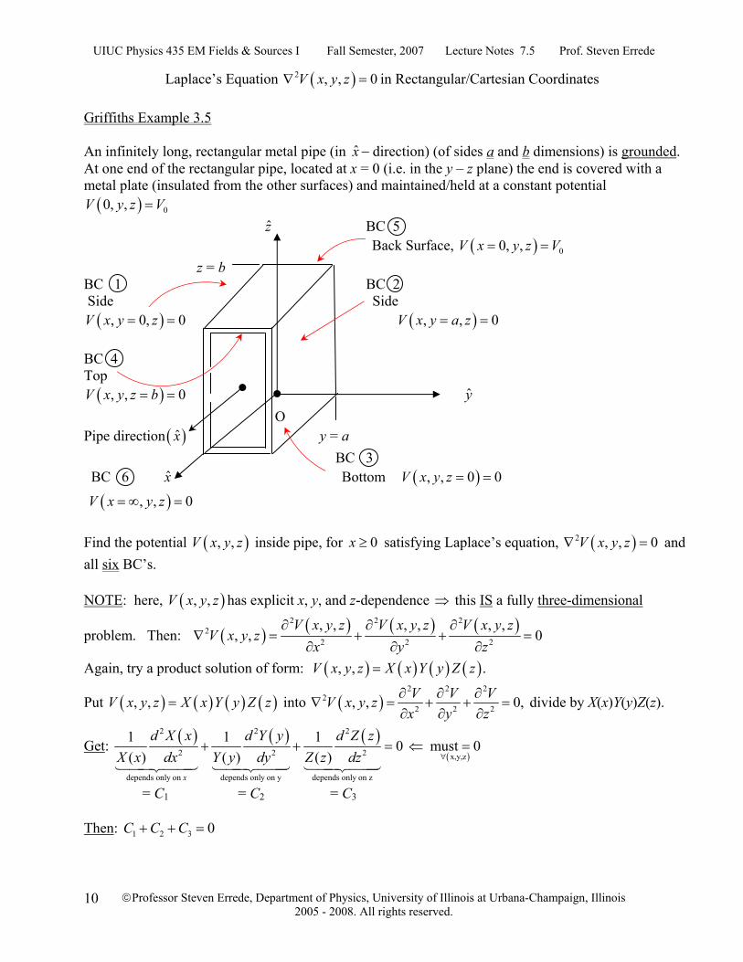
Laplace’s Equation ( )2 , , 0V x y z∇ = in Rectangular/Cartesian Coordinates Griffiths Example 3.5 An infinitely long, rectangular metal pipe (in x − direction) (of sides a and b dimensions) is grounded. At one end of the rectangular pipe, located at x = 0 (i.e. in the y – z plane) the end is covered with a metal plate (insulated from the other surfaces) and maintained/held at a constant potential ( ) 00, ,V y z V=
z BC 5 Back Surface, ( ) 00, ,V x y z V= = z = b BC 1 BC 2
Side Side ( ), 0, 0V x y z= = ( ), , 0V x y a z= =
BC 4 Top ( ), , 0V x y z b= = y
Ο Pipe direction ( )x y = a BC 3 BC 6 x Bottom ( ), , 0 0V x y z = =
( ), , 0V x y z= ∞ =
Find the potential ( ), ,V x y z inside pipe, for 0x ≥ satisfying Laplace’s equation, ( )2 , , 0V x y z∇ = and all six BC’s. NOTE: here, ( ), ,V x y z has explicit x, y, and z-dependence ⇒ this IS a fully three-dimensional
problem. Then: ( ) ( ) ( ) ( )2 2 22
2 2 2
, , , , , ,, , 0
V x y z V x y z V x y zV x y z
x y z∂ ∂ ∂
∇ = + + =∂ ∂ ∂
Again, try a product solution of form: ( ) ( ) ( ) ( ), , .V x y z X x Y y Z z=
Put ( ) ( ) ( ) ( ), ,V x y z X x Y y Z z= into ( )2 2 2
22 2 2, , 0,V V VV x y z
x y z∂ ∂ ∂
∇ = + + =∂ ∂ ∂
divide by X(x)Y(y)Z(z).
Get: ( ) ( ) ( )( )
2 2 2
2 2 2 x,y,z
depends only on depends only on y depends only on z
1 1 1 0 must 0( ) ( ) ( )
x
d X x d Y y d Z zX x dx Y y dy Z z dz ∀
+ + = ⇐ =
= C1 = C2 = C3 Then: 1 2 3 0C C C+ + =
UIUC Physics 435 EM Fields & Sources I Fall Semester, 2007 Lecture Notes 7.5 Prof. Steven Errede
©Professor Steven Errede, Department of Physics, University of Illinois at Urbana-Champaign, Illinois 2005 - 2008. All rights reserved.
11
( )( )
( )( )
( )( )2 2 2
1 2 32 2 2
1 1 1 d X x d Y y d Z z
C C CX x dx Y y dy Z z dz
⇒ = = =
From previous experience e.g. with Griffiths Examples 3.3 and 3.4:
Choose C1 > 0 and C2 < 0, C3 < 0 i.e. 2 21 2 3 C C C k= − − = + , with
22
23
C k
C
⎧ ⎫= −⎪ ⎪⎨ ⎬
= −⎪ ⎪⎩ ⎭
Then:
( ) ( ) ( )2
2 22 0
d X xk X x
dx− + = ( ) ( )
22
2 0d Y y
k Y ydy
+ = ( ) ( )2
22 0
d Z zZ z
dz+ =
General solutions for X(x), Y(y), Z(z) are:
( )( ) ( )( ) ( ) ( )
( ) ( ) ( )
2 2 2 2
sin cos( ) ( , , )
sin cos
k x k xX x Ae Be
Y y C ky D ky V x y z X x Y y Z z
Z z E z F z
+ − + ⎫= +⎪⎪= + =⎬⎪= + ⎪⎭
with boundary conditions: 1) ( ) ( )( )Left Side: , 0, 0 i.e. 0 0V x y z Y y= = = =
2) ( ) ( )( )Right Side: , , 0 i.e. 0V x y a z Y y a= = = =
3) Bottom: ( ) ( )( ) , , 0 0 i.e. 0 0V x y z Z z= = = =
4) Top: ( ) ( )( ) , , 0 i.e. 0V x y z b Z z b= = = =
5) Back: ( ) ( )( )0 0 0, , i.e. 0V x y z V X x V= = = =
6) x →∞ : ( ) ( )( ) , , 0 i.e. 0V x y z X x= ∞ = = ∞ = BC’s 1) and 2) require:
D = 0 and ( ) ( )sin sinka mπ= i.e. , 1, 2,3,nnk naπ⎛ ⎞= =⎜ ⎟
⎝ ⎠…
BC’s 3) and 4) require:
F = 0 and ( ) ( )sin sinb mπ= i.e. , 1, 2,3,mm mbπ⎛ ⎞= =⎜ ⎟
⎝ ⎠…
BC 6) requires: A = 0 Absorbing constants B & E into C, we have:
( ) ( ) ( )2 2
, ,, , sin sinn mk xn m n m n mV x y z C e k y y− +=
with , 1, 2,3,nnk naπ⎛ ⎞= =⎜ ⎟
⎝ ⎠… and , 1, 2,3,m
m mbπ⎛ ⎞= =⎜ ⎟
⎝ ⎠…
UIUC Physics 435 EM Fields & Sources I Fall Semester, 2007 Lecture Notes 7.5 Prof. Steven Errede
©Professor Steven Errede, Department of Physics, University of Illinois at Urbana-Champaign, Illinois 2005 - 2008. All rights reserved.
12
Then: ⇐ General specific ` solution to Laplace’s equation Now BC 5) is ( ) 0
00, , , 1V y z V e−= =
( ) ( ) ( )0 ,1 1
, 1, 2,3, 0, , sin sin with
, 1, 2,3,
n
n m n mn m
m
nk na
V y z V C k y zm mb
π
π
∞ ∞
= =
⎛ ⎞⎛ ⎞= =⎜ ⎟⎜ ⎟⎝ ⎠⎜ ⎟∴ = =⎜ ⎟⎛ ⎞= =⎜ ⎟⎜ ⎟
⎝ ⎠⎝ ⎠
∑∑…
…
Multiply both sides of this equation by ( ) ( )sin sin , n.b. are not necessarily = !!!n m
n nk y z
m m′ ′
′⎛ ⎞ ⎛ ⎞⎜ ⎟ ⎜ ⎟′⎝ ⎠ ⎝ ⎠
and then integrate both sides over y and z, from (y = 0 to y = a) and (z = 0 to z = b) projecting out the Cm,n coefficients by taking this inner product:
( ) ( ) ( ) ( ) ( ) ( )0 0 0 0 01 1
sin sin sin sin sin sina b a b
n m nm n n m mn m
V dy dz k y z C dy dz k y k y z z∞ ∞
′ ′ ′ ′= =
= ×∑∑∫ ∫ ∫ ∫
( ) ( )1
0 0
1 1cos cos2 2
a b
o n m nm nn mmnn m
a bV k y z Ck
δ δ∞
′ ′=
⎧ ⎫⎛ ⎞⎛ ⎞⎪ ⎪ ⎛ ⎞ ⎛ ⎞⎜ ⎟⎜ ⎟′ ′= − − =⎨ ⎬ ⎜ ⎟ ⎜ ⎟⎜ ⎟⎜ ⎟′ ′ ⎝ ⎠ ⎝ ⎠⎪ ⎪⎝ ⎠⎝ ⎠⎩ ⎭
∑
( )( ) ( )( )1 cos 1 cos4o nm nn mm
a b abV n m Cn m
π π δ δπ π ′ ′
⎛ ⎞ ⎛ ⎞ ⎛ ⎞′ ′= − − =⎜ ⎟ ⎜ ⎟ ⎜ ⎟′ ′⎝ ⎠ ⎝ ⎠ ⎝ ⎠
using and n mn mka bπ π
′ ′
′ ′⎛ ⎞⎛ ⎞ ⎛ ⎞= =⎜ ⎟ ⎜ ⎟⎜ ⎟⎝ ⎠ ⎝ ⎠⎝ ⎠
Now: ( )( ) { } ( )( ) { }0 for even # 0 for even #
2 for odd # 2 for odd #1 cos and 1 cosn mn mn mπ π= == =− = − =
4 ab
∴( )( ) o
abn m Vπ π
= for , = odd integers: 1,3,5,4 nmC n m
⎛ ⎞⎜ ⎟⎝ ⎠
…
Or: , 02
16 for , odd integers: 1,3,5 .n mC V n mnmπ
= = …
( ) ( ) ( ) ( )2 2
, ,1 1 1 1
, , , , sin sin
with: , 1, 2,3,
and:
n mk xn m n m n m
n m n m
n
m
V x y z V x y z C e k y z
nk namb
π
π
∞ ∞ ∞ ∞− +
= = = =
= =
⎛ ⎞= =⎜ ⎟⎝ ⎠⎛=
∑∑ ∑∑
…
, 1, 2,3,m⎞ =⎜ ⎟⎝ ⎠
…
UIUC Physics 435 EM Fields & Sources I Fall Semester, 2007 Lecture Notes 7.5 Prof. Steven Errede
©Professor Steven Errede, Department of Physics, University of Illinois at Urbana-Champaign, Illinois 2005 - 2008. All rights reserved.
13
Thus, for this problem the final fully-specified solution for V(x,y,z) satisfying Laplace’s Equation 2 ( , , ) 0V x y z∇ = and all six boundary conditions is:
( ) ( )2 2
02
odd # even #
16 1( , , ) sin sin , n mk xn m n m
n m
V n mV x y z e k y z knm a b
π ππ
∞ ∞− +
= =
⎛ ⎞ ⎛ ⎞= = =⎜ ⎟⎜ ⎟⎝ ⎠⎝ ⎠
∑ ∑
Let ( ) ( ), 2 1 , 2 1 respectively, then:n m i j→ + +
( )( )
( ) ( ) ( ) ( )
( ) ( )
2 22 22 1 / 2 1 / 02
1
16 1 2 1 2 1( , , ) sin sin2 1 2 1
2 1 2 1 with: , 1, 2,3, 1, 2,3,
i a j b x
i j i
i j
V i y j zV x y z e a bi j
i jk i j
a b
π π ππ
π π
∞ ∞− + + +
= =
+ +⎛ ⎞ ⎛ ⎞⎛ ⎞= ⎜ ⎟ ⎜ ⎟ ⎜ ⎟+ +⎝ ⎠ ⎝ ⎠ ⎝ ⎠
+ +⎛ ⎞ ⎛ ⎞= = = =⎜ ⎟ ⎜ ⎟⎝ ⎠ ⎝ ⎠
∑∑
… …
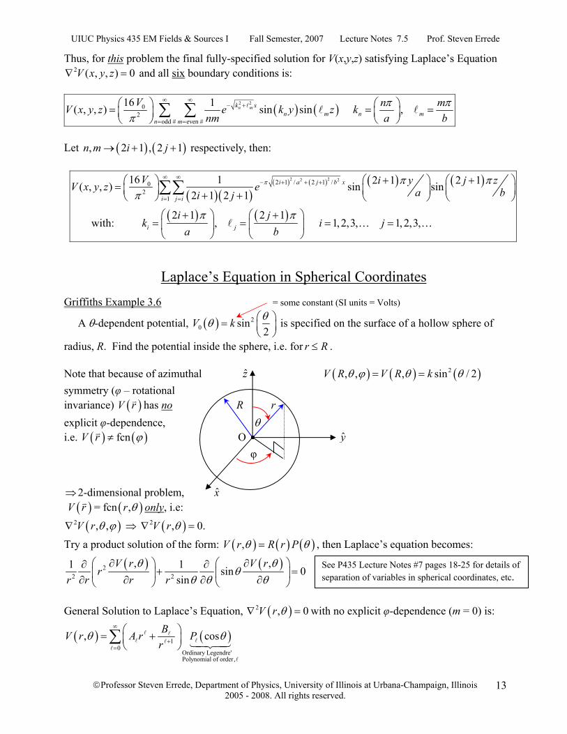
Laplace’s Equation in Spherical Coordinates Griffiths Example 3.6 = some constant (SI units = Volts)
A θ-dependent potential, ( ) 20 sin
2V k θθ ⎛ ⎞= ⎜ ⎟
⎝ ⎠ is specified on the surface of a hollow sphere of
radius, R. Find the potential inside the sphere, i.e. for r R≤ . Note that because of azimuthal z ( ) ( ) ( )2, , , sin / 2V R V R kθ ϕ θ θ= = symmetry (φ – rotational invariance) ( )V r has no R r explicit φ-dependence, θ i.e. ( ) ( )fcnV r ϕ≠ O y φ ⇒2-dimensional problem, x ( ) ( )= fcn ,V r r θ only, i.e:
( ) ( )2 2, , , 0.V r V rθ ϕ θ∇ ⇒ ∇ =
Try a product solution of the form: ( ) ( ) ( ),V r R r Pθ θ= , then Laplace’s equation becomes:
( ) ( )22 2
, ,1 1 sin 0sin
V r V rr
r r r rθ θ
θθ θ θ
∂ ∂⎛ ⎞ ⎛ ⎞∂ ∂+ =⎜ ⎟ ⎜ ⎟∂ ∂ ∂ ∂⎝ ⎠ ⎝ ⎠
General Solution to Laplace’s Equation, ( )2 , 0V r θ∇ = with no explicit φ-dependence (m = 0) is:
( ) ( )10
Ordinary Legendre' Polynomial of order,
, cosBV r A r Pr
θ θ∞
+=
⎛ ⎞= +⎜ ⎟⎝ ⎠
∑
See P435 Lecture Notes #7 pages 18-25 for details of separation of variables in spherical coordinates, etc.

UIUC Physics 435 EM Fields & Sources I Fall Semester, 2007 Lecture Notes 7.5 Prof. Steven Errede
©Professor Steven Errede, Department of Physics, University of Illinois at Urbana-Champaign, Illinois 2005 - 2008. All rights reserved.
14
Now apply BC’s: BC 0 : V ( ),r θ must be finite @ r = 0 (no charges @ origin!)
⇒ 0B = ( ) = for all ∀ ∀ BC 1 :
( ) ( )2
0
, sin cos2
V r R k A R Pθθ θ∞
=
⎛ ⎞= = =⎜ ⎟⎝ ⎠
∑
In order to determine the A coefficients, take inner product – i.e. multiply both sides of this equation by ( ) ( )cos P θ′ ′ ≠ and integrate over θ ( )with cos sind dθ θ θ= from ( )0 to θ θ π= = - i.e. project
out the :sA ′ (n.b. ′ not necessarily = )
( ) ( ) ( )2
0 00
22 1
sin cos sin cos cos sin2
k P d A R P P dπ π
δ
θ θ θ θ θ θ θ θ∞
′=
⎛ ⎞ ′=⎜ ⎟+⎝ ⎠
⎛ ⎞ ′∗ =⎜ ⎟⎝ ⎠
∑∫ ∫ (Kroenecker δ-fcn)
0 if
Kroenecker - fcn1 if
δ δ′
′= ≠⎧ ⎫⎨ ⎬′= =⎩ ⎭
( ) 2
0
2 cos sin sin2 1 2
A R k P dπ θθ θ θ⎛ ⎞ ⎛ ⎞∴ =⎜ ⎟ ⎜ ⎟+⎝ ⎠ ⎝ ⎠∫
Or: ( ) 2
0
2 1 cos sin sin2 2
A k P dR
π θθ θ θ+⎛ ⎞ ⎛ ⎞= ⎜ ⎟ ⎜ ⎟⎝ ⎠ ⎝ ⎠∫
Now:
( )2 1sin 1 cos2 2θ θ⎛ ⎞ = −⎜ ⎟⎝ ⎠
using the half-angle formula
( ) ( )( ) ( )( )
00 1
1
cos 11 cos cos 2 cos cos
PP P
P
θθ θ
θ θ
=⎛ ⎞= − ⎜ ⎟⎜ ⎟=⎝ ⎠
( ) ( ) ( )( )
( ) ( )( ) ( ) ( )( )0 1
0 10
10 0
2 21 3
2 1 1 cos cos cos sin2 2
2 1 cos cos sin cos cos sin4 o
A k P P P dR
k P P d P P dR
π
π π
δ δ
θ θ θ θ θ
θ θ θ θ θ θ θ θ
⎛ ⎞ ⎛ ⎞= =⎜ ⎟ ⎜ ⎟⎝ ⎠ ⎝ ⎠
+⎛ ⎞ ⎛ ⎞∴ = −⎜ ⎟ ⎜ ⎟⎝ ⎠ ⎝ ⎠
⎡ ⎤⎢ ⎥
+⎛ ⎞ ⎢ ⎥= −⎜ ⎟ ⎢ ⎥⎝ ⎠⎢ ⎥⎣ ⎦
∫
∫ ∫
0 02 2k kAR
⎛ ⎞ ⎛ ⎞= =⎜ ⎟ ⎜ ⎟⎝ ⎠ ⎝ ⎠
and 1 1 ,2 2k kAR R
⎛ ⎞ ⎛ ⎞= − = −⎜ ⎟ ⎜ ⎟⎝ ⎠ ⎝ ⎠
all other ( )0 for 1 i.e. 2 .A = > ≥
The fully-specified solution ( ),V r θ satisfying Laplace’s Eqn ( )2 , 0 and the BC's is given by:V r θ∇ =
( ) ( ) ( )0 10 0 1 1 0 1, cos cos , 2, 2V r A r P A r P A k A k Rθ θ θ= + = = −
Or: ( ), 1 cos2k rV r
Rθ θ⎡ ⎤⎛ ⎞ ⎛ ⎞= −⎜ ⎟ ⎜ ⎟⎢ ⎥⎝ ⎠ ⎝ ⎠⎣ ⎦
for r R≤ with the BC: ( ) 2, sin .2
V R k θθ ⎛ ⎞= ⎜ ⎟⎝ ⎠
UIUC Physics 435 EM Fields & Sources I Fall Semester, 2007 Lecture Notes 7.5 Prof. Steven Errede
©Professor Steven Errede, Department of Physics, University of Illinois at Urbana-Champaign, Illinois 2005 - 2008. All rights reserved.
15
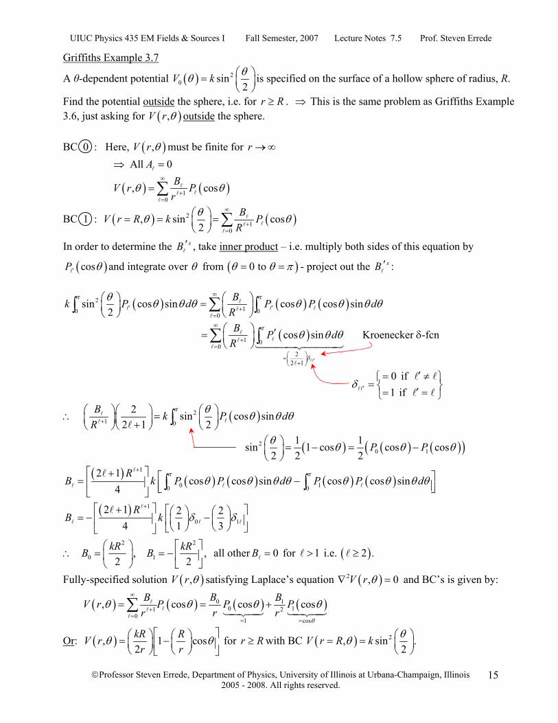
Griffiths Example 3.7
A θ-dependent potential ( ) 20 sin
2V k θθ ⎛ ⎞= ⎜ ⎟
⎝ ⎠is specified on the surface of a hollow sphere of radius, R.
Find the potential outside the sphere, i.e. for r R≥ . ⇒ This is the same problem as Griffiths Example 3.6, just asking for ( ),V r θ outside the sphere. BC 0 : Here, ( ),V r θ must be finite for r →∞ All 0A⇒ =
( ) ( )10
, cosBV r Pr
θ θ∞
+=
=∑
BC 1 : ( ) ( )21
0
, sin cos2
BV r R k PR
θθ θ∞
+=
⎛ ⎞= = =⎜ ⎟⎝ ⎠
∑
In order to determine the sB ′ , take inner product – i.e. multiply both sides of this equation by
( )cosP θ′ and integrate over θ from ( )0 to θ θ π= = - project out the sB ′ :
( ) ( ) ( )210 0
0sin cos sin cos cos sin
2Bk P d P P d
Rπ πθ θ θ θ θ θ θ θ
∞
′ ′+=
⎛ ⎞⎛ ⎞ =⎜ ⎟ ⎜ ⎟⎝ ⎠ ⎝ ⎠
∑∫ ∫
( )1 00
22 1
cos sinB P dR
π
δ
θ θ θ
′
∞
+=
⎛ ⎞=⎜ ⎟+⎝ ⎠
⎛ ⎞ ′= ⎜ ⎟⎝ ⎠
∑ ∫ Kroenecker δ-fcn
0 if 1 if
δ ′
′= ≠⎧ ⎫= ⎨ ⎬′= =⎩ ⎭
( )21 0
2 sin cos sin2 1 2
B k P dR
π θ θ θ θ+
⎛ ⎞⎛ ⎞ ⎛ ⎞∴ =⎜ ⎟ ⎜ ⎟⎜ ⎟ +⎝ ⎠ ⎝ ⎠⎝ ⎠ ∫
( ) ( ) ( )( )20 1
1 1sin 1 cos cos cos2 2 2
P Pθ θ θ θ⎛ ⎞ = − = −⎜ ⎟⎝ ⎠
( ) ( ) ( ) ( ) ( )1
0 10 0
2 1cos cos sin cos cos sin
4R
B k P P d P P dπ π
θ θ θ θ θ θ θ θ+⎡ ⎤+ ⎡ ⎤= −⎢ ⎥ ⎢ ⎥⎣ ⎦⎣ ⎦
∫ ∫
( ) 1
0 1
2 1 2 24 1 3
RB k δ δ
+⎡ ⎤+ ⎡ ⎤⎛ ⎞ ⎛ ⎞= − −⎢ ⎥ ⎜ ⎟ ⎜ ⎟⎢ ⎥⎝ ⎠ ⎝ ⎠⎣ ⎦⎣ ⎦
2 2
0 1 , ,2 2
kR kRB B⎛ ⎞ ⎡ ⎤
∴ = = −⎜ ⎟ ⎢ ⎥⎝ ⎠ ⎣ ⎦
all other 0B = for 1> i.e. ( )2 .≥
Fully-specified solution ( ),V r θ satisfying Laplace’s equation ( )2 , 0V r θ∇ = and BC’s is given by:
( ) ( ) ( ) ( )0 10 11 2
01 cos
, cos cos cosBB BV r P P Pr r r
θ
θ θ θ θ∞
+=
= =
= = +∑
Or: ( ), 1 cos2kR RV r
r rθ θ⎡ ⎤⎛ ⎞ ⎛ ⎞= −⎜ ⎟ ⎜ ⎟⎢ ⎥⎝ ⎠ ⎝ ⎠⎣ ⎦
for r R≥ with BC ( ) 2, sin .2
V r R k θθ ⎛ ⎞= = ⎜ ⎟⎝ ⎠
UIUC Physics 435 EM Fields & Sources I Fall Semester, 2007 Lecture Notes 7.5 Prof. Steven Errede
©Professor Steven Errede, Department of Physics, University of Illinois at Urbana-Champaign, Illinois 2005 - 2008. All rights reserved.
16
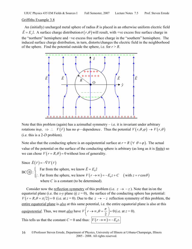
Griffiths Example 3.8 An (initially) uncharged metal sphere of radius R is placed in an otherwise uniform electric field
ˆ.oE E z= A surface charge distribution ( ),rσ θ will result, with +ve excess free surface charge in the “northern” hemisphere and −ve excess free surface charge in the “southern” hemisphere. The induced surface charge distribution, in turn, distorts/changes the electric field in the neighborhood of the sphere. Find the potential outside the sphere, i.e. for r > R.
Note that this problem (again) has a azimuthal symmetry – i.e. it is invariant under arbitrary rotations in ( ), has no dependenceV rϕ ϕ⇒ ∴ − . Thus the potential ( ) ( ), , ,V r V rθ ϕ θ→ (i.e. this is a 2-D problem).
Note also that the conducting sphere is an equipotential surface at r = R ( ) .θ ϕ∀ + The actual value of the potential on the surface of the conducting sphere is arbitrary (as long as it is finite) so we can chose ( ), 0V r R θ= = without loss of generality.
Since ( ) ( )E r V r= −∇
BC 0 : ( ) ( )
0
0
ˆ Far from the sphere, we know Far from the sphere, we know with cos
E E zV r E z C z r θ
⎧ =⎪⎨∴ →∞ = − + =⎪⎩
where is a constant (to be determined).C
Consider now the reflection symmetry of this problem (i.e. z z→ − ). Note that in/on the equatorial plane (i.e. the x-y plane @ z = 0), the surface of the conducting sphere has potential: ( ), 2 0V r R θ π= = = (i.e. at z = 0). Due to the z z→ − reflection symmetry of this problem, the
entire equatorial plane is also at this same potential, i.e. the entire equatorial plane is also at this
equipotential. Thus, we must also have , 02
V r πθ⎛ ⎞→∞ = =⎜ ⎟⎝ ⎠
(i.e. at z = 0).
This tells us that the constant C = 0 and thus: ( ) 0 .V r E z→∞ = −
E E E E
y
z
O R
+ + + + + + + + + + +
− − − − − − − − − − − − −
− − − − − − − − − − − − − − − − − − − − − − − − − − − − −
+ + + + + + + + + + + + + + + + + + + + + + + + + + + + +

UIUC Physics 435 EM Fields & Sources I Fall Semester, 2007 Lecture Notes 7.5 Prof. Steven Errede
©Professor Steven Errede, Department of Physics, University of Illinois at Urbana-Champaign, Illinois 2005 - 2008. All rights reserved.
17
The general solution for the potential, ( ), 0V r θ = in spherical coordinates (for m = 0, i.e. no
φ-dependence) is: ( ) ( ) ( )10 0
, , cosBV r V r A r Pr
θ θ θ∞ ∞
+= =
⎛ ⎞= = +⎜ ⎟⎝ ⎠
∑ ∑
Note that for this problem, the origin ( )0r = is excluded (we want ( ), for , so the 0V r r R Bθ > ≠ in general for such situations). Furthermore, far from the sphere ( ) 0 0, cosV r E z E rθ θ= − = − ( )cosz r θ= , thus we can see that
0A ≠ in general. Apply BC 1 on the surface of sphere:
( ) ( )10
, 0 cosBV r R A R PR
θ θ∞
+=
⎛ ⎞= = = +⎜ ⎟⎝ ⎠
∑
The only way this can be satisfied for all 1(arbitrary) is if: 0 BA RR
θ +⎛ ⎞+ = ∀⎜ ⎟⎝ ⎠
Or: 2 1B R A+= − *
Then: ( ) ( )2 1
10
, cosRV r A r Pr
θ θ+∞
+=
⎛ ⎞⎛ ⎞= −⎜ ⎟⎜ ⎟
⎝ ⎠⎝ ⎠∑
NOTE: for r R the second term in parentheses is negligible. Thus far from sphere we must
have ( ) ( )0 00
,0 cos cosV r E z E r A r Pθ θ∞
=
→∞ = − = − =∑ , and since ( )1 cos cosP θ θ= we don’t
have to bother with inner product “stuff” − we just have to realize that only the 1= term survives in the sum on the RHS!!!
( ) 0 1 1 0 cos cos V r E r A r A Eθ θ∴ →∞ = − = ⇒ = −
∴ 3 31 1 0B R A E R= − = + (from * above).
Thus:
( )
2
3 23
0 0 0 02
2
0 0potential forexternal field potential associated with
electric dipole (1/r pot'l) f
, cos 1 cos cos cos
cos
R R RV r E r E r E r E Rr r r
RE z E Rr
θ θ θ θ θ
θ
⎛ ⎞⎛ ⎞ ⎛ ⎞ ⎛ ⎞= − − = − − = − +⎜ ⎟⎜ ⎟ ⎜ ⎟ ⎜ ⎟⎜ ⎟⎝ ⎠ ⎝ ⎠⎝ ⎠ ⎝ ⎠
⎛ ⎞= − + ⎜ ⎟⎝ ⎠
( )
( ) ( )
rom r, on cond. sphere
, ,ext sphereV r V r
σ θ
θ θ= +
We can now calculate/determine the surface charge density ( )σ θ on surface of conducting sphere:
( ) ( ) 3
0 0 0 0
,1 2 cos 3 cos
r R r R
V r RE Er rθ
σ θ ε ε θ ε θ= =
⎛ ⎞∂ ⎛ ⎞= − = + =⎜ ⎟⎜ ⎟⎜ ⎟∂ ⎝ ⎠⎝ ⎠
Note that ( ) 0σ θ > in the “northern” hemisphere and that ( )0 0σ < in the “southern” hemisphere.
UIUC Physics 435 EM Fields & Sources I Fall Semester, 2007 Lecture Notes 7.5 Prof. Steven Errede
©Professor Steven Errede, Department of Physics, University of Illinois at Urbana-Champaign, Illinois 2005 - 2008. All rights reserved.
18
Griffiths Example 3.9 A specified surface charge density ( )0 coskσ θ θ= is “glued” over the surface of a spherical shell of radius R. Find the resulting potential inside and outside the sphere.
[n.b. We could do this problem by direct integration of ( ) ( )0
0
1, ,4
V r dAσ θ
θπε
= ∫ r but we’ll use
the Laplace equation series solution method instead…] Here again, note that we have azimuthal symmetry (i.e. no explicit ϕ-dependence), Thus this is a 2-D problem, i.e. ( ) ( ), , , .V r V rθ ϕ θ⇒ First, for r < R (inside sphere):
( ) ( )0
, cosinV r A r Pθ θ∞
=
=∑
(Here, all 0B = because ( )11 @ 0, i.e. 0,r Vr θ+ →∞ = must be finite)
Second, for r > R (outside sphere):
( ) ( )10
, cosoutBV r Pr
θ θ∞
+=
=∑
(Here, all 0A = because r →∞@ ,r →∞ i.e. ( ), 0.V r θ→∞ → The potential ( ),V r R θ= must be continuous @ r = R:
i.e. ( ) ( ), ,in outV r R V r Rθ θ= = =
( ) ( )10 0
cos cosBA R P PR
θ θ∞ ∞
+= =
∴ =∑ ∑
This can only be true θ∀ iff (if and only if):
1
BA RR += , i.e. 2 1B R A+=
Now since the surface charge density ( )0 coskσ θ θ= is glued onto the surface of sphere @ r = R,
the radial derivative of ( ),r R
V r θ=
suffers a discontinuity at this surface
i.e. ( ) ( ) ( )0
0 0
, , cosout in
r R
V r V r kr rθ θ σ θ θ
ε ε=
∂ ∂⎛ ⎞− = − = −⎜ ⎟∂ ∂⎝ ⎠
Then: ( ) ( ) ( )2 1
1 10 0
, cos cosoutB RV r P A P
r rθ θ θ
+∞ ∞
+ += =
⎛ ⎞= = ⎜ ⎟
⎝ ⎠∑ ∑
and: ( ) ( ) 2 1
0
, cos with inV r A r P B R Aθ θ∞
+
=
= =∑
Thus: ( ) ( ) ( ) ( ) ( )2 1
12
0 0
,1 cos 1 cosout
r R r R
V r RA P A R Pr rθ
θ θ+∞ ∞
−+
= == =
∂ ⎛ ⎞= − + = − +⎜ ⎟∂ ⎝ ⎠∑ ∑
UIUC Physics 435 EM Fields & Sources I Fall Semester, 2007 Lecture Notes 7.5 Prof. Steven Errede
©Professor Steven Errede, Department of Physics, University of Illinois at Urbana-Champaign, Illinois 2005 - 2008. All rights reserved.
19
( ) ( ) ( ){ } ( )
( ) ( )
1 1
0
1
0
, , 1 cos
cos 2 1 cos
out in
r R
V r V rA R A R P
r r
kA R P
θ θθ
θθε
∞− −
==
∞−
=−
∂ ∂⎡ ⎤∴ − = − + +⎢ ⎥∂ ∂⎣ ⎦
= − + = −
∑
∑
( )( )1 only the = 1 . . cos cosi e P θ θ⇒ = term is non-zero!! All other & 0 for 1.A B = ≠
( )01 1 1
0
3 cos 3 cos coskA R P Aθ θ θε
∴ − = − = −
∴ 103
kAε
= and 3 31 1
0
13
kB R A Rε
⎛ ⎞= = ⎜ ⎟
⎝ ⎠
Then:
For r < R: ( ) ( ) ( )1 10 0
, cos cos cos3 3ink kV r A rP r z z rθ θ θ θε ε
= = = =
For r > R: ( ) ( )2
112
0
, cos cos3out
B k RV r P Rr r
θ θ θε
⎛ ⎞ ⎛ ⎞= = ⎜ ⎟ ⎜ ⎟⎝ ⎠⎝ ⎠
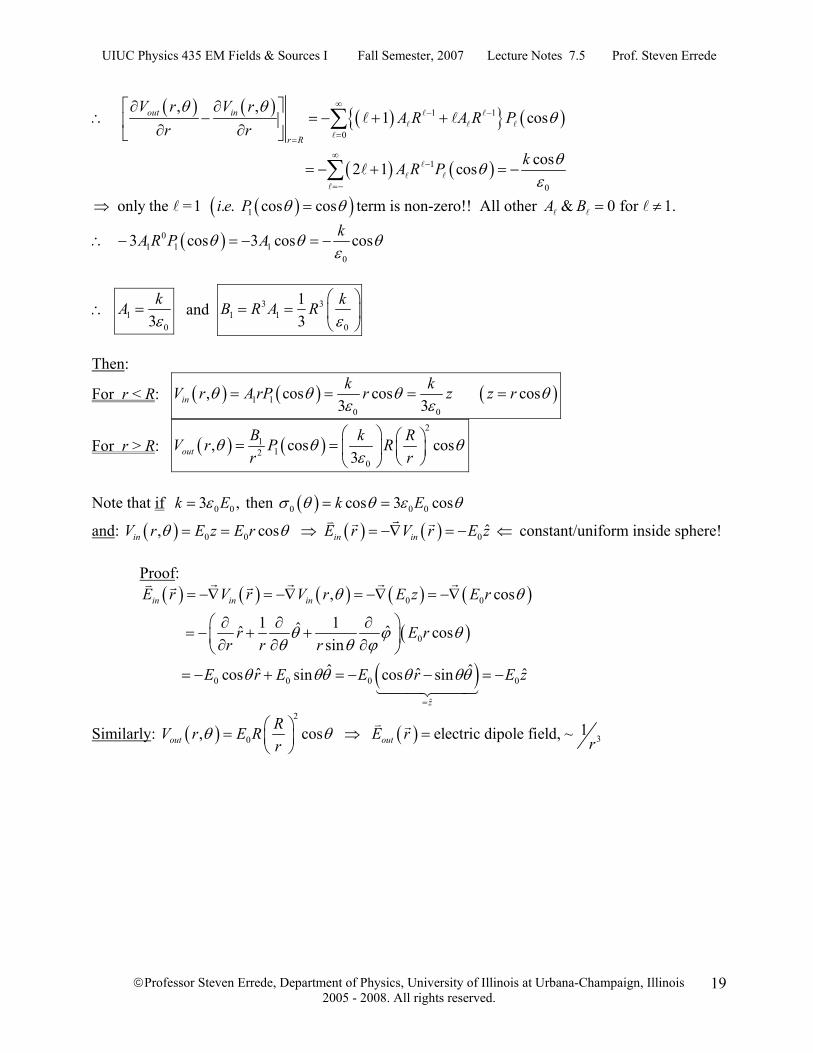
Note that if 0 03 ,k Eε= then ( )0 0 0cos 3 cosk Eσ θ θ ε θ= =
and: ( ) ( ) ( )0 0 0 ˆ, cos in in inV r E z E r E r V r E zθ θ= = ⇒ = −∇ = − ⇐ constant/uniform inside sphere! Proof:
( ) ( ) ( ) ( ) ( )
( )
( )
0 0
0
0 0 0 0
ˆ
, cos
1 1ˆ ˆˆ cossinˆ ˆˆ ˆ ˆ cos sin cos sin
in in in
z
E r V r V r E z E r
r E rr r r
E r E E r E z
θ θ
θ ϕ θθ θ ϕ
θ θθ θ θθ=
= −∇ = −∇ = −∇ = −∇
⎛ ⎞∂ ∂ ∂= − + +⎜ ⎟∂ ∂ ∂⎝ ⎠
= − + = − − = −
Similarly: ( ) ( )2
301, cos electric dipole field, ~out out
RV r E R E r rrθ θ⎛ ⎞= ⇒ =⎜ ⎟
⎝ ⎠
Top Related