


Languages
Pages
Legal


Nikolova 2020 1
LECTURE 18: Horn Antennas
(Rectangular horn antennas. Circular apertures.)
1 Rectangular Horn Antennas
Horn antennas are popular in the microwave bands (above 1 GHz). Horns
provide high gain, low VSWR (with waveguide feeds), relatively wide
bandwidth, and they are not difficult to make. There are three basic types of
rectangular horns.
[Balanis]
The horns can be also flared exponentially. This provides better impedance
match in a broader frequency band. Such horns are more difficult to make, which
means higher cost.
The rectangular horns are ideally suited for rectangular waveguide feeds. The
horn acts as a gradual transition from a waveguide mode to a free-space mode of
the EM wave. When the feed is a cylindrical waveguide, the antenna is usually a
conical horn.
Nikolova 2020 2
Why is it necessary to consider the horns separately instead of applying the
theory of waveguide aperture antennas directly? It is because the so-called phase
error occurs due to the difference between the lengths from the center of the feed
to the center of the horn aperture and the horn edge. The field does not have the
same phase across the horn aperture. This makes the uniform-phase aperture
results invalid for the horns.
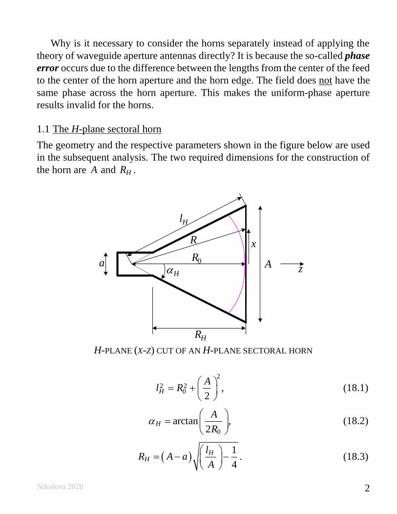
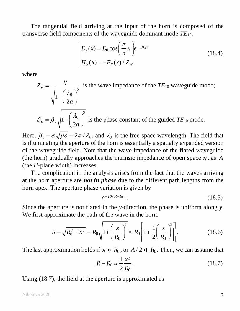
1.1 The H-plane sectoral horn
The geometry and the respective parameters shown in the figure below are used
in the subsequent analysis. The two required dimensions for the construction of
the horn are A and HR .
H-plane (x-z) cut of an H-plane
sectoral horn
a
Hl
HR
0R
R x
A zH
H-PLANE (X-Z) CUT OF AN H-PLANE SECTORAL HORN
2
2 20
2H
Al R
= +
, (18.1)
0
arctan2
H
A
R
=
, (18.2)
( )1
4
HH
lR A a
A
= − −
. (18.3)
Nikolova 2020 3
The tangential field arriving at the input of the horn is composed of the
transverse field components of the waveguide dominant mode TE10:
0( ) cos
( ) ( ) /
gj zy
x y w
E x E x ea
H x E x Z
− =
= −
(18.4)
where
201
2
wZ
a
=
−
is the wave impedance of the TE10 waveguide mode;
20
0 12
ga
= −
is the phase constant of the guided TE10 mode.
Here, 0 02 / = = , and 0 is the free-space wavelength. The field that
is illuminating the aperture of the horn is essentially a spatially expanded version
of the waveguide field. Note that the wave impedance of the flared waveguide
(the horn) gradually approaches the intrinsic impedance of open space , as A
(the H-plane width) increases.
The complication in the analysis arises from the fact that the waves arriving
at the horn aperture are not in phase due to the different path lengths from the
horn apex. The aperture phase variation is given by
0( )j R Re − − . (18.5)
Since the aperture is not flared in the y-direction, the phase is uniform along y.
We first approximate the path of the wave in the horn:
2 2
2 20 00
0 0
11 1
2
x xR R x R R
R R
= + = + +
. (18.6)
The last approximation holds if 0x R , or 0/ 2A R . Then, we can assume that
2
0
0
1
2
xR R
R− . (18.7)
Using (18.7), the field at the aperture is approximated as
Nikolova 2020 4
( )2
020( ) cos /
y
j xR
aE x E x A e
−
. (18.8)
The field at the aperture plane outside the aperture is assumed equal to zero. The
field expression (18.8) is substituted in the integral for EyI (see Lecture 17):
( sin cos sin sin )( , ) ( , )y
A
E j x yy a
S
I E x y e dx dy + = , (18.9)
2
0
/2 /2
sin cos sin sin20
/2 /2
( , )
( , ) cos
A bj x
E j x j yRy
A b
I
I E x e e dx e dyA
+ +−
− −
=
.(18.10)
The second integral has been already encountered. The first integral is
cumbersome and the final result only is given below:
( )
( )0
0
sin 0( , )
.5 sin sin1( , )
2 0.5 sin sinEy
RI E b
bI
b
=
, (18.11)
where
20
20
sin cos2
2 2 1 1
sin cos2
2 2 1 1
( ) ( ) ( ) ( )
( ) (
( , )
) ( ) ( )
Rj
A
Rj
A
e C s jS s C s jS s
e C t jS t C t jS t
I
+
−
= − − +
+ − − +
(18.12)
and
01 0
0
1
2
A Rs R u
R A
= − − −
;
02 0
0
1
2
A Rs R u
R A
= + − −
;
01 0
0
1
2
A Rt R u
R A
= − − +
;
02 0
0
1
2
A Rt R u
R A
= + − +
;
sin cosu = .
Nikolova 2020 5
( )C x and ( )S x are Fresnel integrals, which are defined as
2
0
2
0
( ) cos ; ( ) ( ),2
( ) sin ; ( ) ( ).2
x
x
C x d C x C x
S x d S x S x
= − = −
= − = −
(18.13)
More accurate evaluation of ( , )EyI is obtained if the approximation in
(18.6) is not made, and yaE is substituted in (18.9) as
( )2 2 2 200 0 00 0( ) cos cos
y
j R x R j R xj RaE x E x e E e x e
A A
− + − − ++
= =
. (18.14)
The far field can be calculated from ( , )EyI as (see Lecture 17):
(1 cos )sin ( , ),4
(1 cos )cos ( , ),4
j rEy
j rEy
eE j I
r
eE j I
r
−
−
= +
= +
(18.15)
or
( )
( )
( )
00
sin 0.5 sin sin1 cos
4 2 0.5 sin sin
ˆ ˆ ( , ) sin cos .
j r bR ej E b
r b
I
− + =
+
E
θ φ
(18.16)
The amplitude pattern of the H-plane sectoral horn is obtained as
( )
( )
sin 0.5 sin sin1 cos( , ) ( , )
2 0.5 sin sin
bE I
b
+ =
. (18.17)
Principal-plane patterns
E-plane ( 90 = ): ( )
( )
sin 0.5 sin1 cos( )
2 0.5 sinE
bF
b
+ =
(18.18)
The second factor in (18.18) is dominant and it is identical to the second factor
of the pattern of a slit of width b (along the y-axis).
Nikolova 2020 6
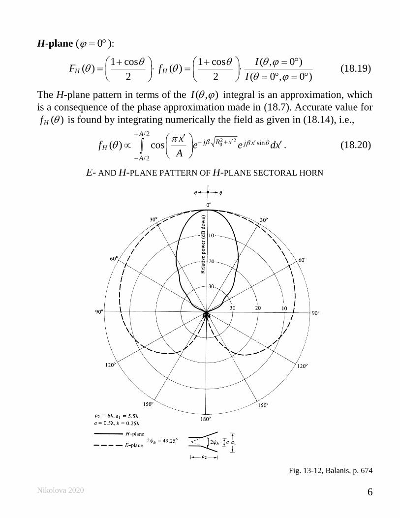
H-plane ( 0 = ):
1 cos 1 cos ( , 0 )
( ) ( )2 2 ( 0 , 0 )
H H
IF f
I
+ + = = =
= = (18.19)
The H-plane pattern in terms of the ( , )I integral is an approximation, which
is a consequence of the phase approximation made in (18.7). Accurate value for
( )Hf is found by integrating numerically the field as given in (18.14), i.e.,
2 20
/2
sin
/2
( ) cos
A
j R x j xH
A
xf e e dx
A
+
− +
−
. (18.20)
E- AND H-PLANE PATTERN OF H-PLANE SECTORAL HORN
Fig. 13-12, Balanis, p. 674
Nikolova 2020 7
The directivity of the H-plane sectoral horn is calculated by the general
directivity expression for apertures (for derivation, see Lecture 17):
2
02 2
4
| |
A
A
aS
aS
dsD
ds
=
E
E. (18.21)
The integral in the denominator is proportional to the total radiated power,
/2 /222 2 2
0 0
/2 /2
2 | | cos | |2
A
b A
rad a
S b A
Abds E x dx dy E
A
+ +
− −
= = =
E . (18.22)
In the solution of the integral in the numerator of (18.21), if the field is substituted
with its phase approximation in (18.8), the result for the directivity of the H-plane
horn is
2
32 4( )H H
H tph ph
b AD Ab
= =
, (18.23)
where
2
8;t
=
2
2 2
1 2 1 2( ) ( ) ( ) ( )64
Hph C p C p S p S p
t
= − + − ;
1 2
1 12 1 , 2 1
8 8p t p t
t t
= + = − +
;
2
0
1 1
8 /
At
R
=
.
The factor t explicitly shows the aperture efficiency associated with the
aperture cosine taper. The factor Hph is the aperture efficiency associated with
the aperture phase distribution.
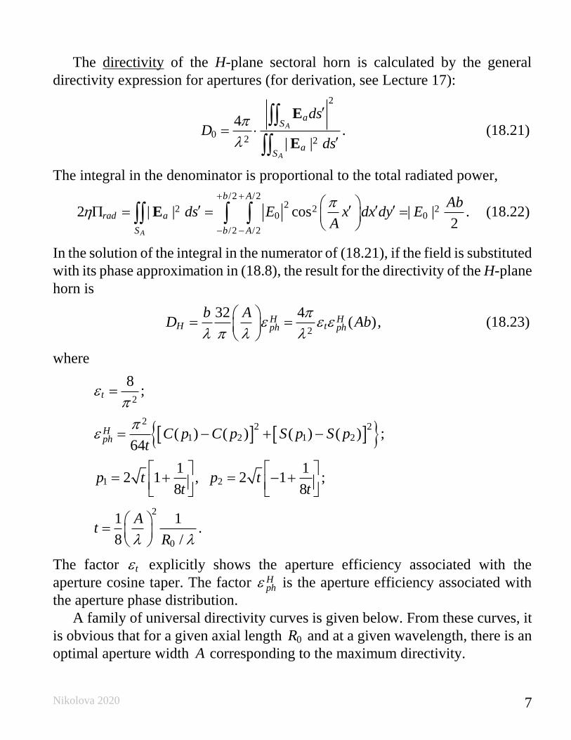
A family of universal directivity curves is given below. From these curves, it
is obvious that for a given axial length 0R and at a given wavelength, there is an
optimal aperture width A corresponding to the maximum directivity.
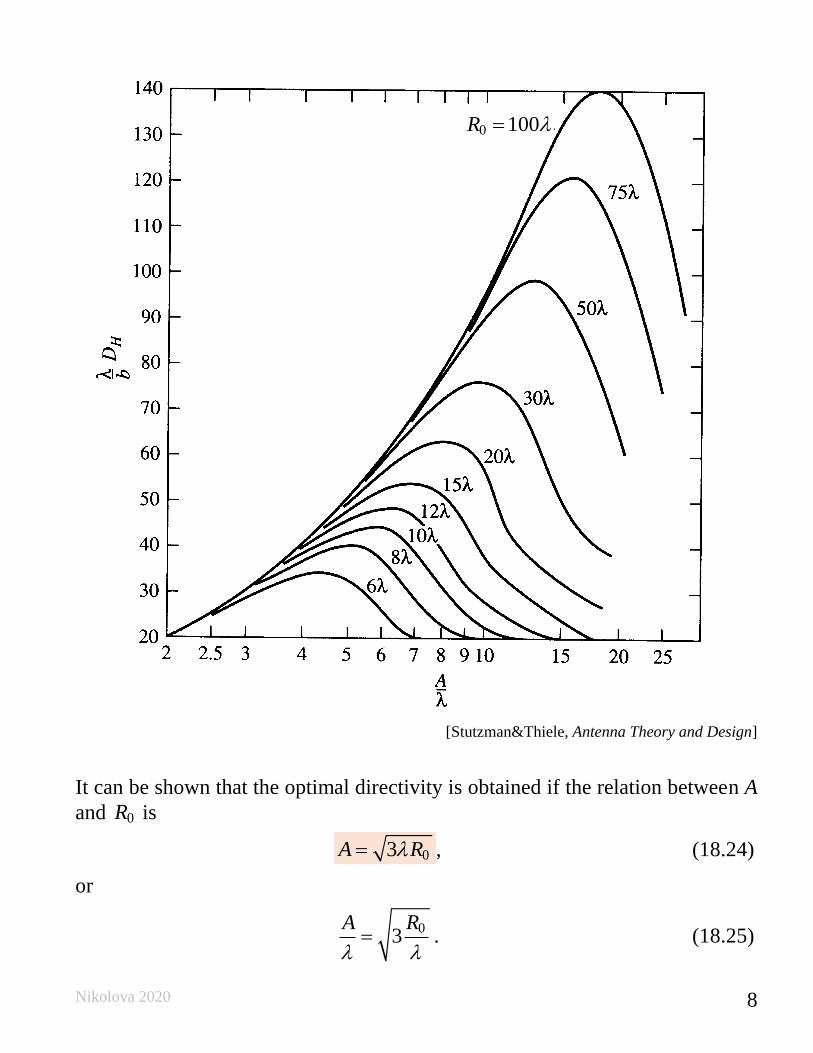
Nikolova 2020 8
[Stutzman&Thiele, Antenna Theory and Design]
It can be shown that the optimal directivity is obtained if the relation between A
and 0R is
03A R= , (18.24)
or
0
3A R
= . (18.25)
0 100R =
Nikolova 2020 9
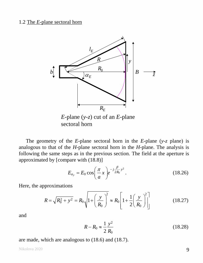
1.2 The E-plane sectoral horn
E-plane (y-z) cut of an E-plane
sectoral horn
b
El
ER
0R
R y
B zE
The geometry of the E-plane sectoral horn in the E-plane (y-z plane) is
analogous to that of the H-plane sectoral horn in the H-plane. The analysis is
following the same steps as in the previous section. The field at the aperture is
approximated by [compare with (18.8)]
2
020 cos
y
j yR
aE E x ea
−
=
. (18.26)
Here, the approximations
2 2
2 20 00
0 0
11 1
2
y yR R y R R
R R
= + = + +
(18.27)
and
2
0
0
1
2
yR R
R− (18.28)
are made, which are analogous to (18.6) and (18.7).
Nikolova 2020 10
The radiation field is obtained as
( )
20
sin sin0 2 20
2 2 1 12
4 ˆ ˆsin cos4
cos sin cos(1 cos ) 2
( ) ( ) ( ) ( ) .2
1 sin cos2
R Bj r ja R ej E e
r
a
C r jS r C r jS ra
− = +
+
− − + −
E θ φ
(18.29)
The arguments of the Fresnel integrals used in (18.29) are
1 0
0
2 0
0
sin sin ,2 2
sin sin .2 2
B Br R
R
B Br R
R
= − −
= + −
(18.30)
Principal-plane patterns
The normalized H-plane pattern is found by substituting 0 = in (18.29):
2
cos sin1 cos 2
( )2
1 sin2
a
Ha
+
=
−
. (18.31)
The second factor in this expression is the pattern of a uniform-phase cosine-
amplitude tapered line source. The normalized E-plane pattern is found by
substituting 90 = in (18.29):
2 22 1 2 1
2 20 0
( ) ( ) ( ) ( )(1 cos ) (1 cos )( ) ( )
2 2 4 ( ) ( )E
C r C r S r S rE f
C r S r
= =
− + −+ += =
+ . (18.32)
Here, the arguments of the Fresnel integrals are calculated for 90 = :
Nikolova 2020 11
1 0
0
2 0
0
sin ,2 2
sin ,2 2
B Br R
R
B Br R
R
= − −
= + −
(18.33)
and
0 2
0
( 0)2
Br r
R
= = = = . (18.34)
Similar to the H-plane sectoral horn, the principal E-plane pattern can be
accurately calculated if no approximation of the phase distribution is made. Then,
the function ( )Ef has to be calculated by numerical integration of (compare
with (18.20))
2 20
/2
sin
/2
( )
B
j R y j yE
B
f e e dy − +
−
. (18.35)
Nikolova 2020 12
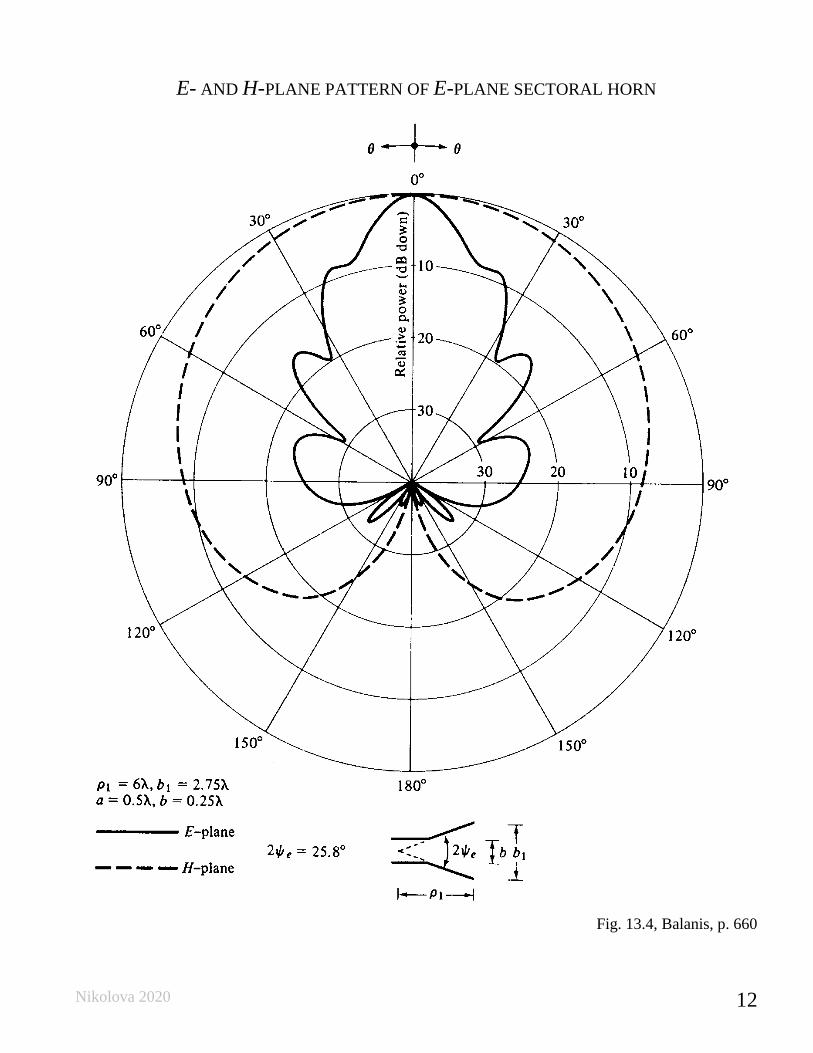
E- AND H-PLANE PATTERN OF E-PLANE SECTORAL HORN
Fig. 13.4, Balanis, p. 660
Nikolova 2020 13
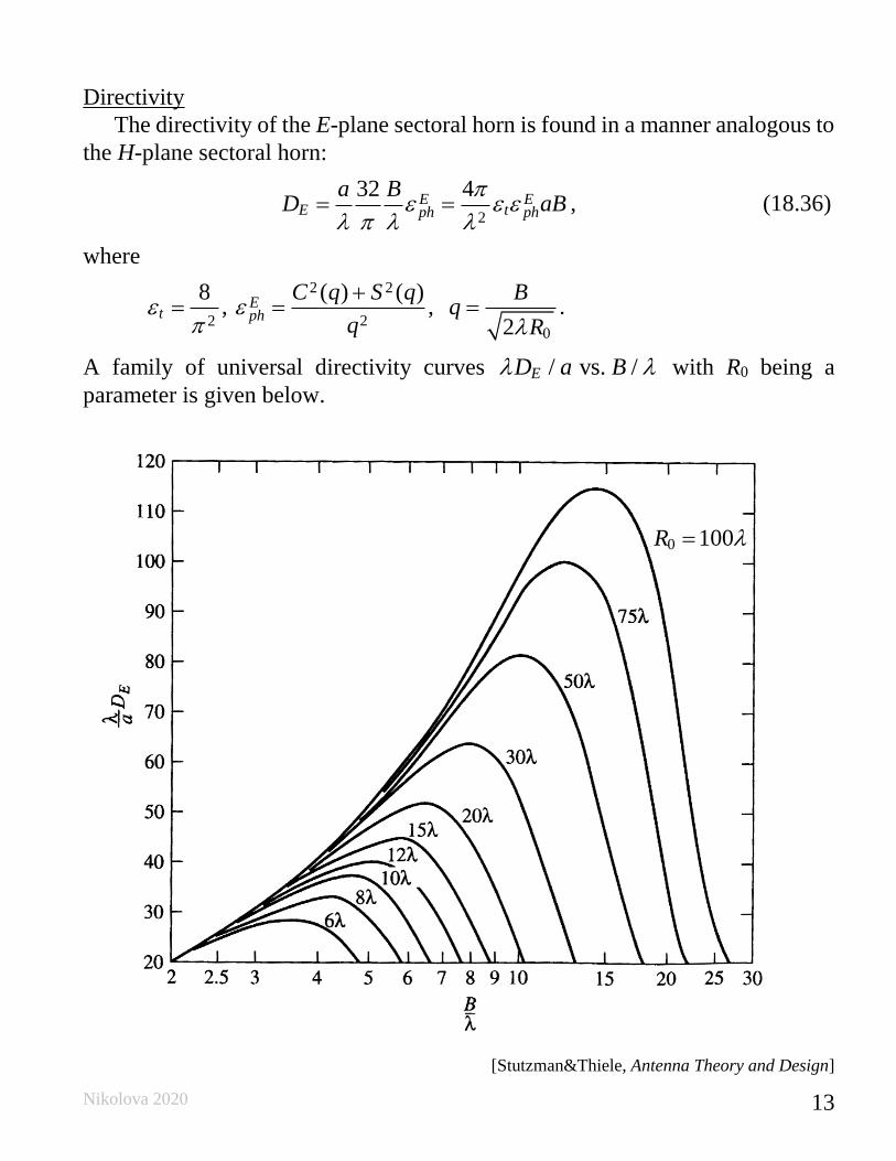
Directivity
The directivity of the E-plane sectoral horn is found in a manner analogous to
the H-plane sectoral horn:
2
32 4E E
E tph ph
a BD aB
= = , (18.36)
where
2
8t
= ,
2 2
20
( ) ( ),
2
Eph
C q S q Bq
q R
+= = .
A family of universal directivity curves / vs. /ED a B with R0 being a
parameter is given below.
[Stutzman&Thiele, Antenna Theory and Design]
0 100R =
Nikolova 2020 14
The optimal relation between the flared height B and the horn apex length 0R
that produces the maximum possible directivity is
02B R= . (18.37)
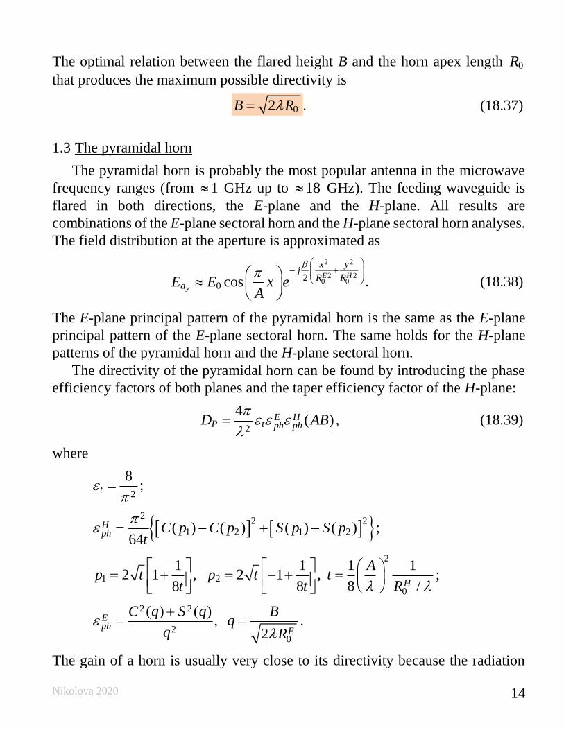
1.3 The pyramidal horn
The pyramidal horn is probably the most popular antenna in the microwave
frequency ranges (from 1 GHz up to 18 GHz). The feeding waveguide is
flared in both directions, the E-plane and the H-plane. All results are
combinations of the E-plane sectoral horn and the H-plane sectoral horn analyses.
The field distribution at the aperture is approximated as
2 2
2 20 02
0 cosE H
y
x yj
R RaE E x e
A
− +
. (18.38)
The E-plane principal pattern of the pyramidal horn is the same as the E-plane
principal pattern of the E-plane sectoral horn. The same holds for the H-plane
patterns of the pyramidal horn and the H-plane sectoral horn.
The directivity of the pyramidal horn can be found by introducing the phase
efficiency factors of both planes and the taper efficiency factor of the H-plane:
2
4( )E H
P t ph phD AB
= , (18.39)
where
2
8t
= ;
2
2 2
1 2 1 2( ) ( ) ( ) ( )64
Hph C p C p S p S p
t
= − + − ;
1 2
1 12 1 , 2 1 ,
8 8p t p t
t t
= + = − +
2
0
1 1
8 /H
At
R
=
;
2 2
20
( ) ( ),
2
Eph
E
C q S q Bq
q R
+= = .
The gain of a horn is usually very close to its directivity because the radiation
Nikolova 2020 15
efficiency is very good (low losses). The directivity as calculated with (18.39) is
very close to measurements. The above expression is a physical optics
approximation, and it does not take into account only multiple diffractions, and
the diffraction at the edges of the horn arising from reflections from the horn
interior. These phenomena, which are unaccounted for, lead to only very minor
fluctuations of the measured results about the prediction of (18.39). That is why
horns are often used as gain standards in antenna measurements.
The optimal directivity of an E-plane horn is achieved at 1q = [see also
(18.37)], 0.8Eph = . The optimal directivity of an H-plane horn is achieved at
3 / 8t = [see also (18.24)], 0.79Hph = . Thus, the optimal horn has a phase
aperture efficiency of
0.632P H Eph ph ph = = . (18.40)
The total aperture efficiency includes the taper factor, too:
0.81 0.632 0.51P H Etph ph ph = = = . (18.41)
Therefore, the best achievable directivity for a rectangular waveguide horn is
about half that of a uniform rectangular aperture.
We reiterate that best accuracy is achieved if Hph and E
ph are calculated
numerically without using the second-order phase approximation as in (18.38).
Optimum horn design
Usually, the optimum (from the point of view of maximum gain) design of a
horn is desired because it results in the shortest axial length for a given gain. The
whole design can be actually reduced to the solution of a single fourth-order
equation. For a horn to be realizable, the following must be true:
E H PR R R= = . (18.42)
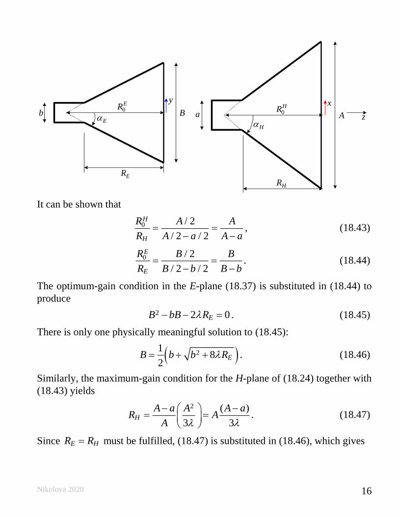
The figures below summarize the notations used in describing the horn’s
geometry.
Nikolova 2020 16
z
HR
0HR
x
A
Hab
ER
0ER
y
BE
It can be shown that
0 / 2
/ 2 / 2
H
H
R A A
R A a A a= =
− −, (18.43)
0 / 2
/ 2 / 2
E
E
R B B
R B b B b= =
− −. (18.44)
The optimum-gain condition in the E-plane (18.37) is substituted in (18.44) to
produce
2 2 0EB bB R− − = . (18.45)
There is only one physically meaningful solution to (18.45):
( )21
82
EB b b R= + + . (18.46)
Similarly, the maximum-gain condition for the H-plane of (18.24) together with
(18.43) yields
2 ( )
3 3H
A a A A aR A
A
− − = =
. (18.47)
Since E HR R= must be fulfilled, (18.47) is substituted in (18.46), which gives
Nikolova 2020 17
21 8 ( )
2 3
A A aB b b
−= + +
. (18.48)
Substituting in the expression for the horn’s gain,
2
4apG AB
= , (18.49)
gives the relation between A, the gain G, and the aperture efficiency ap :
2
2
4 1 8 ( )
2 3ap
A a aG A b b
−= + +
, (18.50)
2 2 4
4 3
2 2
3 30
8 32ap ap
bG GA aA A
− + − = . (18.51)
Equation (18.51) is the optimum pyramidal horn design equation. The optimum-
gain value of 0.51ap = is usually used, which makes the equation a fourth-order
polynomial equation in A. Its roots can be found analytically (which is not
particularly easy) and numerically. In a numerical solution, the first guess is
usually set at (0) 0.45A G= . Once A is found, B can be computed from (18.48)
and E HR R= is computed from (18.47).
Sometimes, an optimal horn is desired for a known axial length R0. In this
case, there is no need for nonlinear-equation solution. The design procedure
follows the steps: (a) find A from (18.24), (b) find B from (18.37), and (c)
calculate the gain G using (18.49) where 0.51ap = .
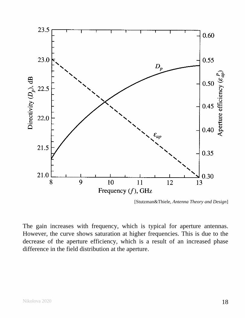
Horn antennas operate well over a bandwidth of 50%. However, gain
performance is optimal only at a given frequency. To understand better the
frequency dependence of the directivity and the aperture efficiency, the plot of
these curves for an X-band (8.2 GHz to 12.4 GHz) horn fed by WR90 waveguide
is given below ( 0.9a = in. = 2.286 cm and 0.4b = in. = 1.016 cm).
Nikolova 2020 18
[Stutzman&Thiele, Antenna Theory and Design]
The gain increases with frequency, which is typical for aperture antennas.
However, the curve shows saturation at higher frequencies. This is due to the
decrease of the aperture efficiency, which is a result of an increased phase
difference in the field distribution at the aperture.
Nikolova 2020 19
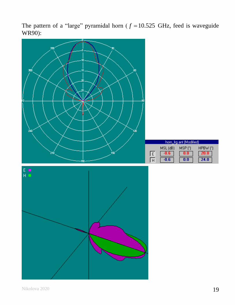
The pattern of a “large” pyramidal horn ( 10.525f = GHz, feed is waveguide
WR90):

Nikolova 2020 20
Comparison of the E-plane patterns of a waveguide open end, “small” pyramidal
horn and “large” pyramidal horn:
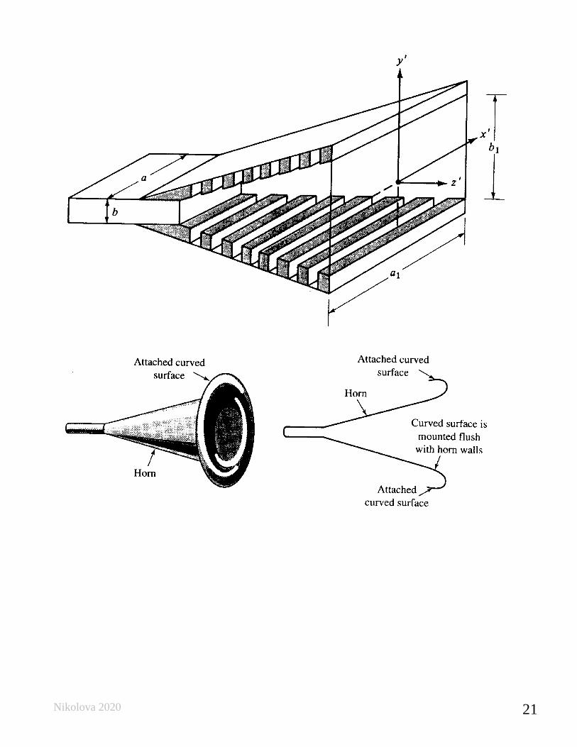
Note the multiple side lobes and the significant back lobe. They are due to
diffraction at the horn edges, which are perpendicular to the E field. To reduce
edge diffraction, enhancements are proposed for horn antennas such as
• corrugated horns
• aperture-matched horns
The corrugated horns achieve tapering of the E field in the vertical direction,
thus, reducing the side-lobes and the diffraction from the top and bottom edges.
The overall main beam becomes smooth and nearly rotationally symmetrical
(esp. for A B ). This is important when the horn is used as a feed to a reflector
antenna.
Nikolova 2020 21
Nikolova 2020 22
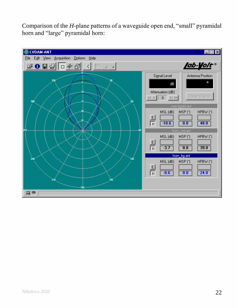
Comparison of the H-plane patterns of a waveguide open end, “small” pyramidal
horn and “large” pyramidal horn:
Nikolova 2020 23
2 Circular apertures
2.1 A uniform circular aperture
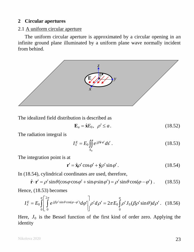
The uniform circular aperture is approximated by a circular opening in an
infinite ground plane illuminated by a uniform plane wave normally incident
from behind.
x
y
z
Ea
The idealized field distribution is described as
0ˆ ,a E a= E x . (18.52)
The radiation integral is
ˆ0
a
E jx
S
I E e ds = r r . (18.53)
The integration point is at
ˆ ˆcos sin = +r x y . (18.54)
In (18.54), cylindrical coordinates are used, therefore,
ˆ sin (cos cos sin sin ) sin cos( ) . = + = −r r (18.55)
Hence, (18.53) becomes
2
sin cos( )0 0 0
0 0 0
2 ( sin )
a a
E jxI E e d d E J d
−
= = . (18.56)
Here, 0J is the Bessel function of the first kind of order zero. Applying the
identity
Nikolova 2020 24
0 1( ) ( )xJ x dx xJ x= (18.57)
to (18.56) leads to
0 12 ( sin )sin
Ex
aI E J a
= . (18.58)
Note that in this case the equivalent magnetic current formulation of the
equivalence principle is used [see Lecture 17]. The far field is obtained as
( )
( ) 120
ˆ ˆcos cos sin2
2 ( sin )ˆ ˆcos cos sin .2 sin
j rEx
j r
ej I
r
e J aj E a
r a
= − =
= −
E θ φ
θ φ
(18.59)
Principal-plane patterns
E-plane ( 0 = ): 12 ( sin )
( )sin
J aE
a
= (18.60)
H-plane ( 90 = ): 12 ( sin )
( ) cossin
J aE
a
= (18.61)
The 3-D amplitude pattern:
12 2
( )
2 ( sin )( , ) 1 sin sin
sin
f
J aE
a
= − (18.62)
The larger the aperture, the less significant the cos factor is in (18.61) because
the main beam in the 0 = direction is very narrow and in this small solid angle
cos 1 . Thus, the 3-D pattern of a large circular aperture features a fairly
symmetrical beam.
Nikolova 2020 25
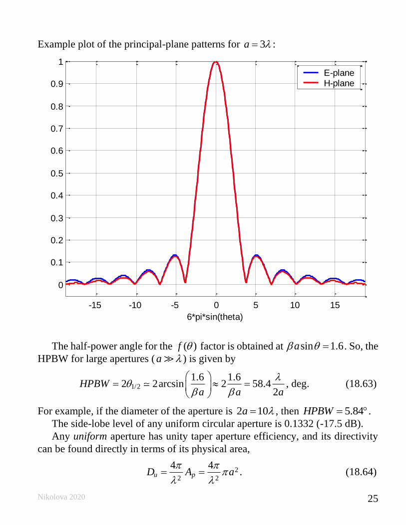
Example plot of the principal-plane patterns for 3a = :
The half-power angle for the ( )f factor is obtained at sin 1.6a = . So, the
HPBW for large apertures (a ) is given by
1/2
1.6 1.62 2arcsin 2 58.4
2HPBW
a a a
= =
, deg. (18.63)
For example, if the diameter of the aperture is 2 10a = , then 5.84HPBW = .
The side-lobe level of any uniform circular aperture is 0.1332 (-17.5 dB).
Any uniform aperture has unity taper aperture efficiency, and its directivity
can be found directly in terms of its physical area,
2
2 2
4 4u pD A a
= = . (18.64)
-15 -10 -5 0 5 10 15
0
0.1
0.2
0.3
0.4
0.5
0.6
0.7
0.8
0.9
1
6*pi*sin(theta)
E-planeH-plane
Nikolova 2020 26
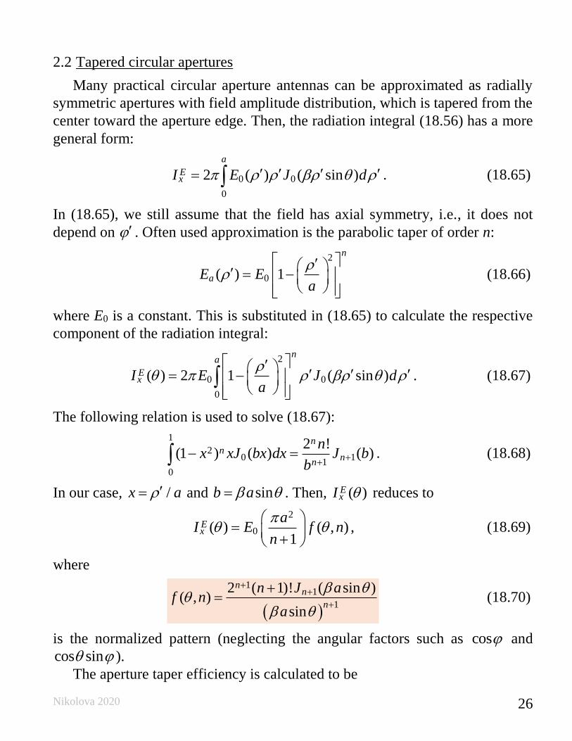
2.2 Tapered circular apertures
Many practical circular aperture antennas can be approximated as radially
symmetric apertures with field amplitude distribution, which is tapered from the
center toward the aperture edge. Then, the radiation integral (18.56) has a more
general form:
0 0
0
2 ( ) ( sin )
a
ExI E J d = . (18.65)
In (18.65), we still assume that the field has axial symmetry, i.e., it does not
depend on . Often used approximation is the parabolic taper of order n:
2
0( ) 1
n
aE Ea
= −
(18.66)
where E0 is a constant. This is substituted in (18.65) to calculate the respective
component of the radiation integral:
2
0 0
0
( ) 2 1 ( sin )
na
ExI E J d
a
= −
. (18.67)
The following relation is used to solve (18.67):
1
20 1
10
2 !(1 ) ( ) ( )
nn
nn
nx xJ bx dx J b
b+
+− = . (18.68)
In our case, /x a= and sinb a = . Then, ( )ExI reduces to
2
0( ) ( , )1
Ex
aI E f n
n
=
+ , (18.69)
where
( )
11
1
2 ( 1)! ( sin )( , )
sin
nn
n
n J af n
a
++
+
+= (18.70)
is the normalized pattern (neglecting the angular factors such as cos and
cos sin ).
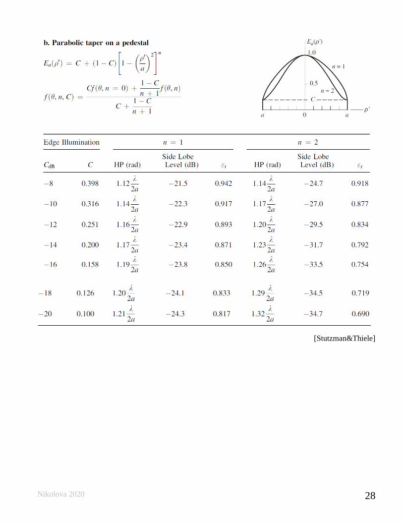
The aperture taper efficiency is calculated to be
Nikolova 2020 27
2
22
1
1
2 (1 ) (1 )
1 2 1
t
CC
n
C C CC
n n
− + +
=− −
+ ++ +
. (18.71)
Here, C denotes the pedestal height. The pedestal height is the edge field
illumination relative to the illumination at the center.
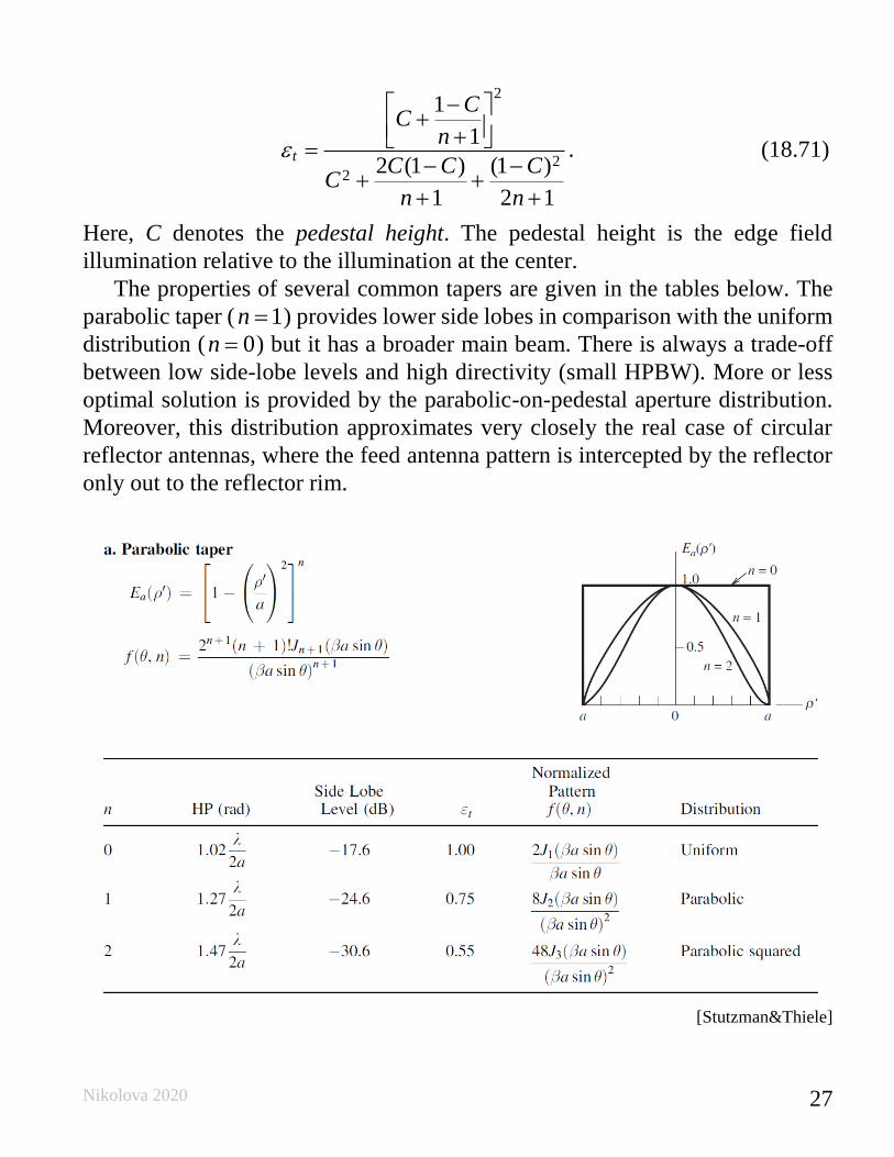
The properties of several common tapers are given in the tables below. The
parabolic taper ( 1n = ) provides lower side lobes in comparison with the uniform
distribution ( 0n = ) but it has a broader main beam. There is always a trade-off
between low side-lobe levels and high directivity (small HPBW). More or less
optimal solution is provided by the parabolic-on-pedestal aperture distribution.
Moreover, this distribution approximates very closely the real case of circular
reflector antennas, where the feed antenna pattern is intercepted by the reflector
only out to the reflector rim.
[Stutzman&Thiele]
Nikolova 2020 28
[Stutzman&Thiele]
Top Related