


Languages
Pages
Legal

Lecture 14 Image Compression
1. What and why image compression2 B i t2. Basic concepts 3. Encoding/decoding, entropy
What is Data and Image Compression?
Data compression is the art and science of representing information in a compact forminformation in a compact form.
Data is a sequence of symbols taken from a discrete
l h b talphabet.
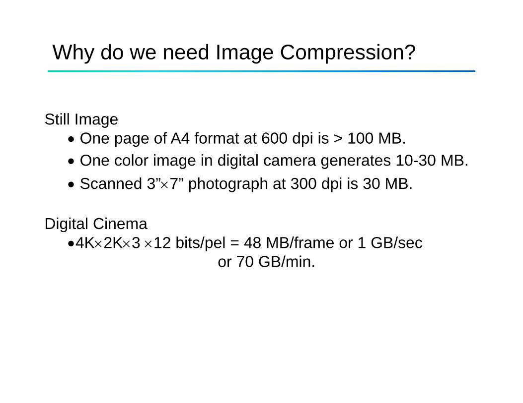
Why do we need Image Compression?
Still Imageg• One page of A4 format at 600 dpi is > 100 MB. • One color image in digital camera generates 10-30 MB. • Scanned 3”×7” photograph at 300 dpi is 30 MB.
Digital CinemaDigital Cinema•4K×2K×3 ×12 bits/pel = 48 MB/frame or 1 GB/sec
or 70 GB/min.
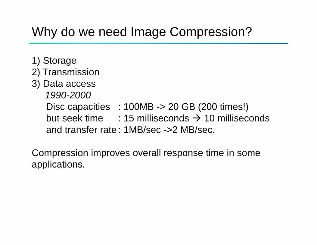
Why do we need Image Compression?
1) Storage2) Transmission)3) Data access
1990-2000Disc capacities : 100MB -> 20 GB (200 times!)Disc capacities : 100MB -> 20 GB (200 times!)but seek time : 15 milliseconds 10 millisecondsand transfer rate : 1MB/sec ->2 MB/sec.
Compression improves overall response time in some applications.pp
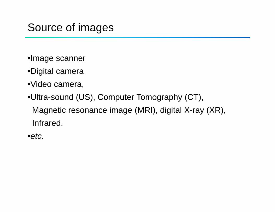
Source of images
•Image scanner •Digital camera •Video camera,•Ultra-sound (US), Computer Tomography (CT),Magnetic resonance image (MRI), digital X-ray (XR),Infrared.
•etc.
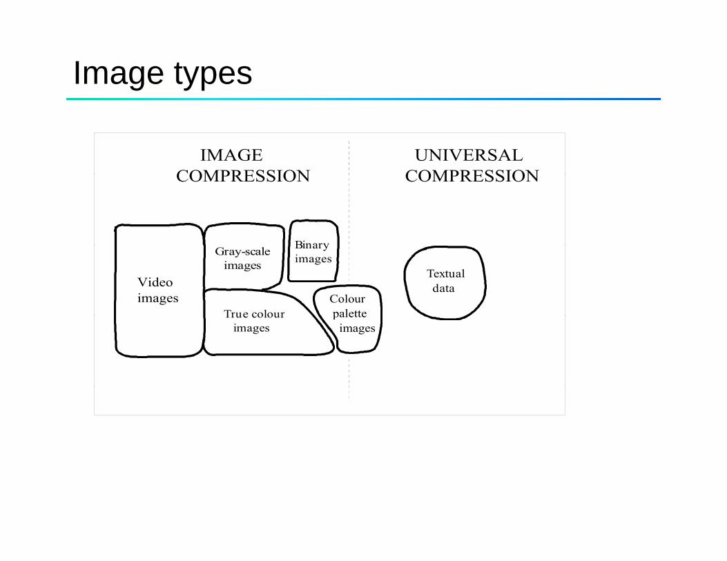
Image types
IMAGECOMPRESSION
UNIVERSALCOMPRESSIONCOMPRESSION COMPRESSION
Binary
Videoimages
Gray-scale images
True colour
Binaryimages
Colourpalette
Textual data
True colour images
palette images
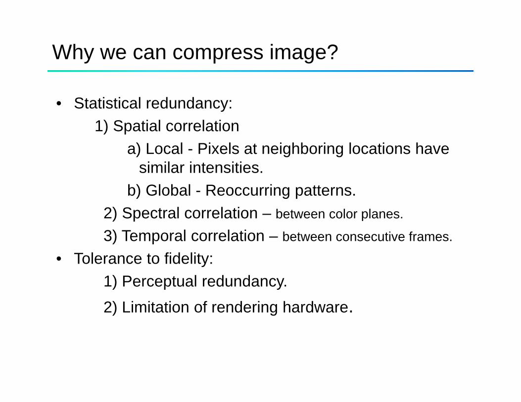
Why we can compress image?
• Statistical redundancy:1) Spatial correlation1) Spatial correlation
a) Local - Pixels at neighboring locations have similar intensities.
b) Global - Reoccurring patterns.2) Spectral correlation – between color planes.
3) Temporal correlation – between consecutive frames.
• Tolerance to fidelity:1) P t l d d1) Perceptual redundancy.2) Limitation of rendering hardware.
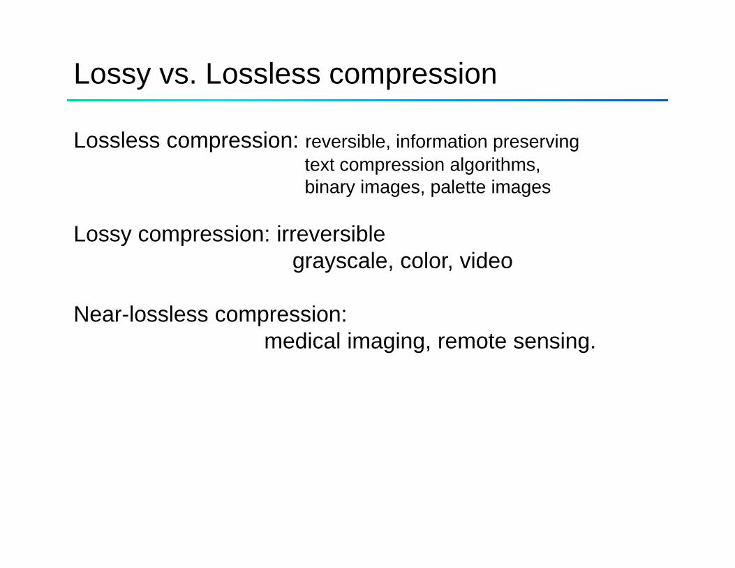
Lossy vs. Lossless compression
Lossless compression: reversible, information preservingtext compression algorithms, binary images, palette images
Lossy compression: irreversible grayscale, color, video
Near-lossless compression:Near lossless compression: medical imaging, remote sensing.
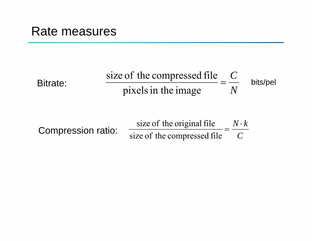
Rate measures
CfilecompressedtheofsizeBitrate:
NC
=image in the pixels
filecompressedtheofsizebits/pel
Compression ratio: CkN ⋅
=filecompressedtheofsize
file original theof sizeCfilecompressedtheofsize
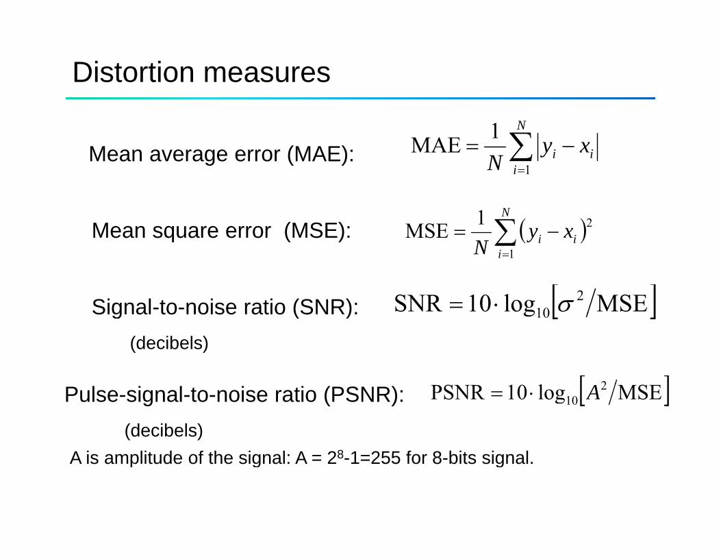
Distortion measures
Mean average error (MAE): ∑=
−=N
iii xy
N 1
1MAEi 1
Mean square error (MSE): ( )∑ −=N
ii xyN
21MSE ( )∑=iN 1
Signal-to-noise ratio (SNR): [ ]MSElog10SNR 210 σ⋅=
[ ]2
Signal to noise ratio (SNR): [ ]g10
(decibels)
[ ]MSElog10PSNR 210 A⋅=Pulse-signal-to-noise ratio (PSNR):
(decibels)A is amplit de of the signal A 28 1 255 for 8 bits signalA is amplitude of the signal: A = 28-1=255 for 8-bits signal.
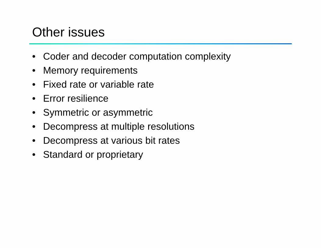
Other issues
• Coder and decoder computation complexity• Memory requirements• Fixed rate or variable rate• Error resilience• Symmetric or asymmetric• Decompress at multiple resolutions• Decompress at various bit rates• Decompress at various bit rates• Standard or proprietary
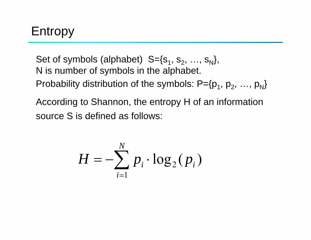
Entropy
Set of symbols (alphabet) S={s1, s2, …, sN},N is number of symbols in the alphabet. y pProbability distribution of the symbols: P={p1, p2, …, pN}
According to Shannon, the entropy H of an informationAccording to Shannon, the entropy H of an informationsource S is defined as follows:
∑ ⋅−=N
ii ppH 2 )(log∑=i
ii pp1
2 )(g
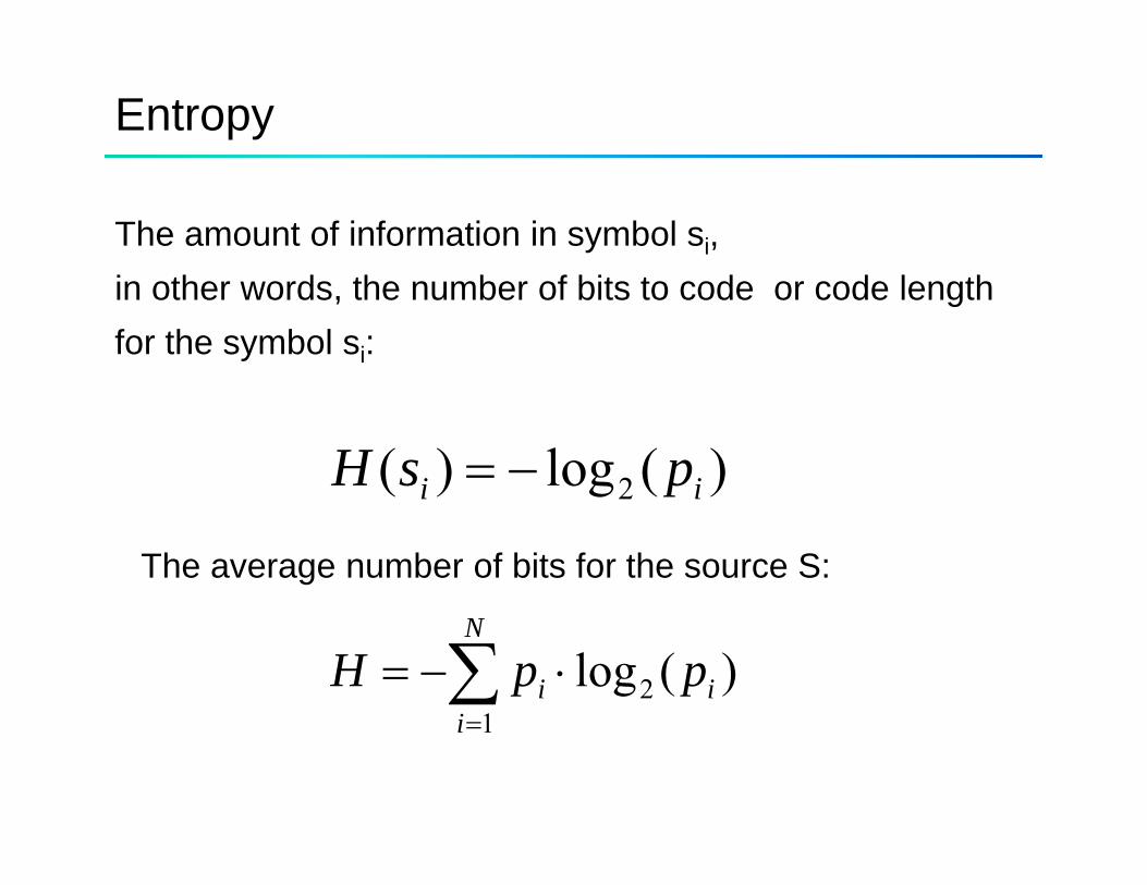
Entropy
The amount of information in symbol si, i h d h b f bi d d l hin other words, the number of bits to code or code lengthfor the symbol si:
)(log)( 2 ii psH −= 2 ii
The average number of bits for the source S:
∑ ⋅−=N
iii ppH
12 )(log
=i 1
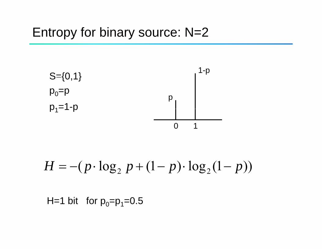
Entropy for binary source: N=2
S={0 1} 1-pS {0,1}p0=pp1=1-p
pp1 1 p
0 1
))1(log)1(log( 22 ppppH −⋅−+⋅−= ))(g)(g( 22 pppp
H=1 bit for p0=p1=0.5H 1 bit for p0 p1 0.5
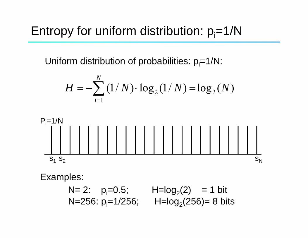
Entropy for uniform distribution: pi=1/N
Uniform distribution of probabilities: pi=1/N:
)(log)/1(log)/1( 21
2 NNNHN
i∑
=
=⋅−=
Pi=1/N
s1 s2 sN
Examples: N= 2: pi=0.5; H=log2(2) = 1 bitpi ; g2( )N=256: pi=1/256; H=log2(256)= 8 bits
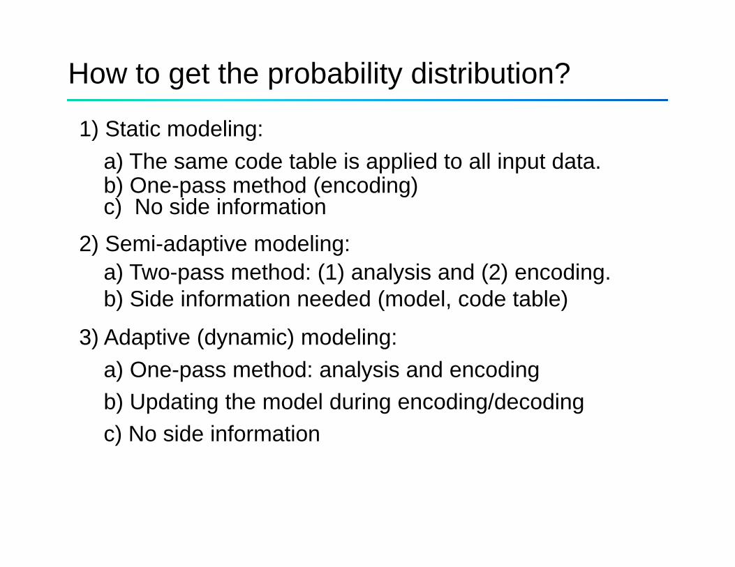
How to get the probability distribution?
1) Static modeling:a) The same code table is applied to all input data. b) One-pass method (encoding)c) No side information
2) Semi-adaptive modeling:2) Semi adaptive modeling:a) Two-pass method: (1) analysis and (2) encoding.b) Side information needed (model, code table)
3) Adaptive (dynamic) modeling:a) One-pass method: analysis and encodingb) Updating the model during encoding/decodingc) No side information
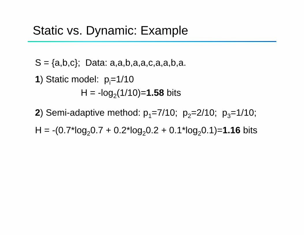
Static vs. Dynamic: Example
S = {a,b,c}; Data: a,a,b,a,a,c,a,a,b,a.
1) Static model: pi=1/10H = -log2(1/10)=1.58 bits
2) Semi-adaptive method: p1=7/10; p2=2/10; p3=1/10;
H = -(0.7*log20.7 + 0.2*log20.2 + 0.1*log20.1)=1.16 bitsH (0.7 log20.7 0.2 log20.2 0.1 log20.1) 1.16 bits
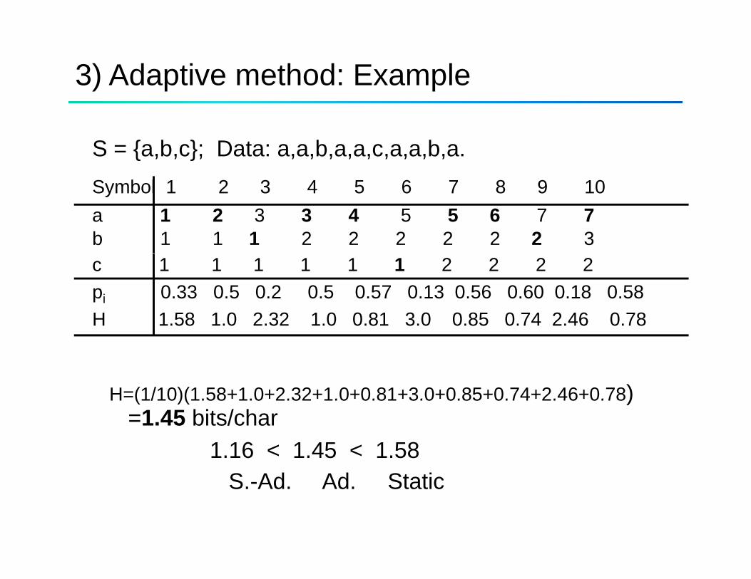
3) Adaptive method: Example
S = {a,b,c}; Data: a,a,b,a,a,c,a,a,b,a.S b l 1 2 3 4 5 6 7 8 9 10Symbol 1 2 3 4 5 6 7 8 9 10 a 1 2 3 3 4 5 5 6 7 7b 1 1 1 2 2 2 2 2 2 3c 1 1 1 1 1 1 2 2 2 2pi 0.33 0.5 0.2 0.5 0.57 0.13 0.56 0.60 0.18 0.58H 1.58 1.0 2.32 1.0 0.81 3.0 0.85 0.74 2.46 0.78
H=(1/10)(1.58+1.0+2.32+1.0+0.81+3.0+0.85+0.74+2.46+0.78)H (1/10)(1.58 1.0 2.32 1.0 0.81 3.0 0.85 0.74 2.46 0.78)=1.45 bits/char
1.16 < 1.45 < 1.58S.-Ad. Ad. Static
Coding methods
• Shannon-Fano Coding• Huffman Coding• Predictive coding• Block coding
• Arithmetic code• Golomb-Rice codes
Shannon-Fano Code: A top-down approach
1) Sort symbols according their probabilities:) y g pp1 ≤ p2 ≤ … ≤ pN
2) R i l di id i t t h ith th2) Recursively divide into parts, each with approx. the samenumber of counts (probability)
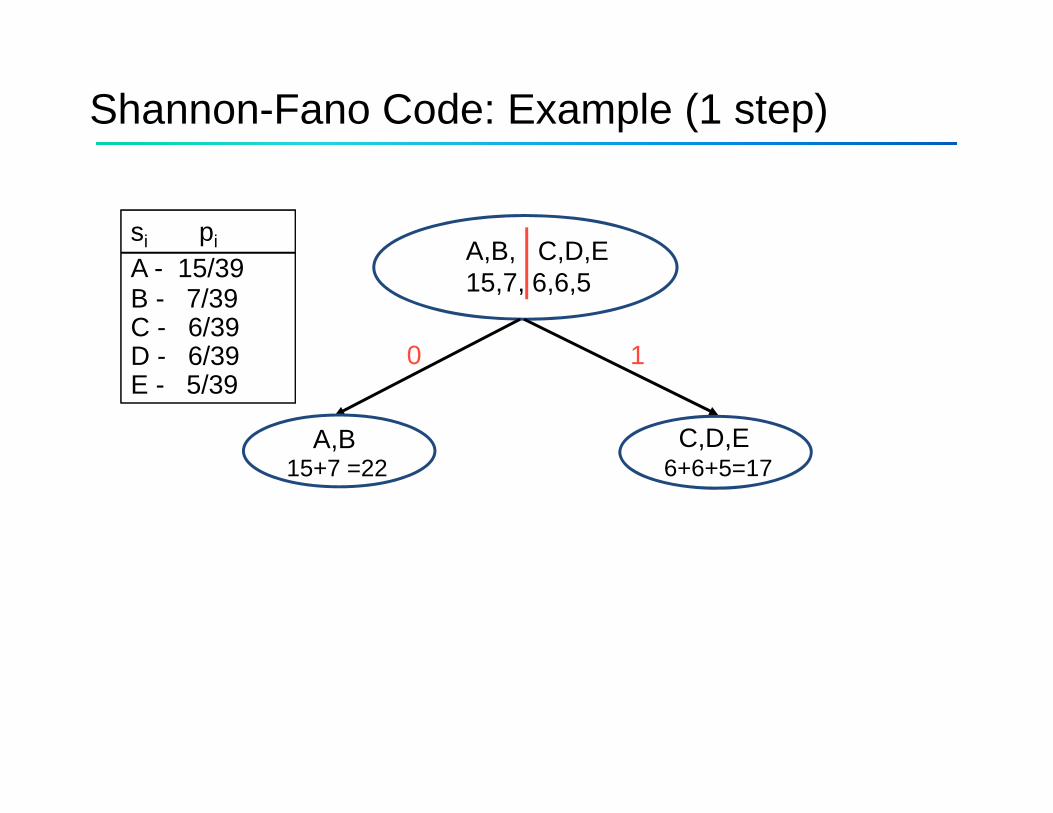
Shannon-Fano Code: Example (1 step)
si pi A B C D EA - 15/39B - 7/39 C - 6/39 D 6/39
A,B, C,D,E15,7, 6,6,5
0 1D - 6/39E - 5/39
A,B C,D,E
0 1
15+7 =22 6+6+5=17
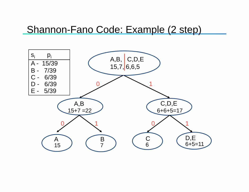
Shannon-Fano Code: Example (2 step)
si pi A B C D EA - 15/39B - 7/39 C - 6/39 D 6/39
A,B, C,D,E15,7, 6,6,5
0 1D - 6/39E - 5/39
A,B C,D,E
0 1
15+7 =22 6+6+5=17
0 01 1
A15
B7
C6
D,E6+5=11
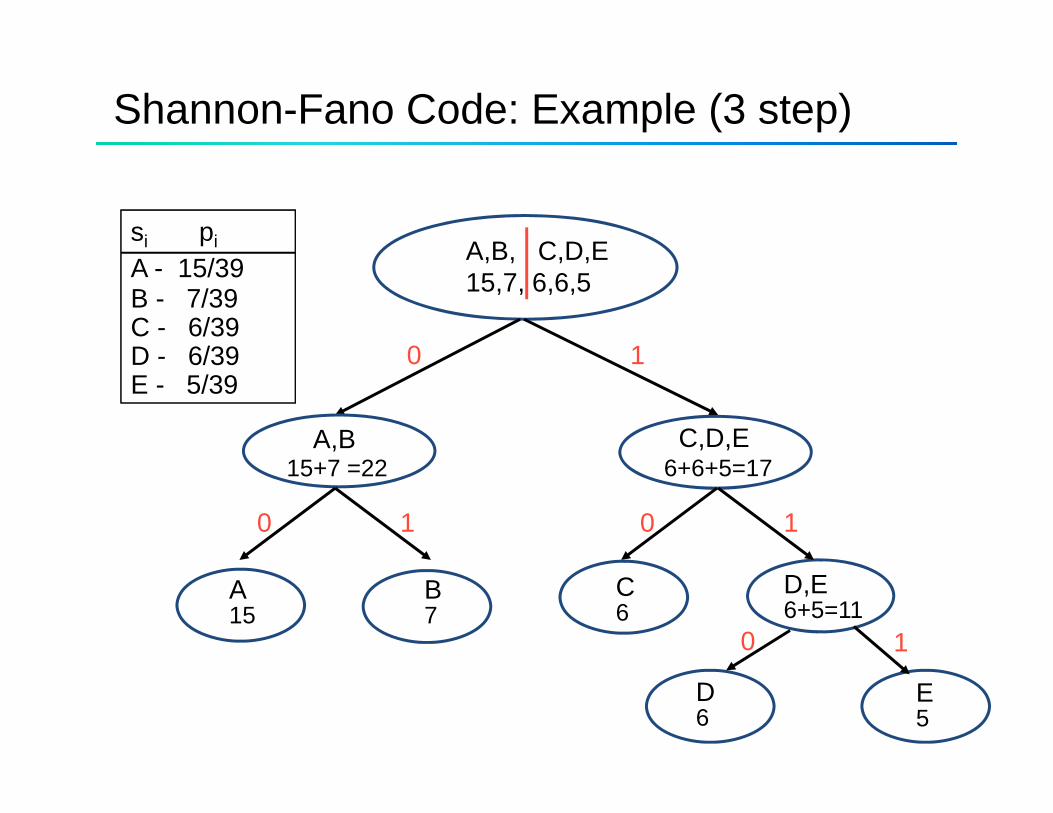
Shannon-Fano Code: Example (3 step)
si pi A B C D EA - 15/39B - 7/39 C - 6/39 D 6/39
A,B, C,D,E15,7, 6,6,5
0 1D - 6/39E - 5/39
A,B C,D,E
0 1
15+7 =22 6+6+5=17
0 1 0 1
A15
B7
C6
D,E6+5=11
0 1
D6
E5
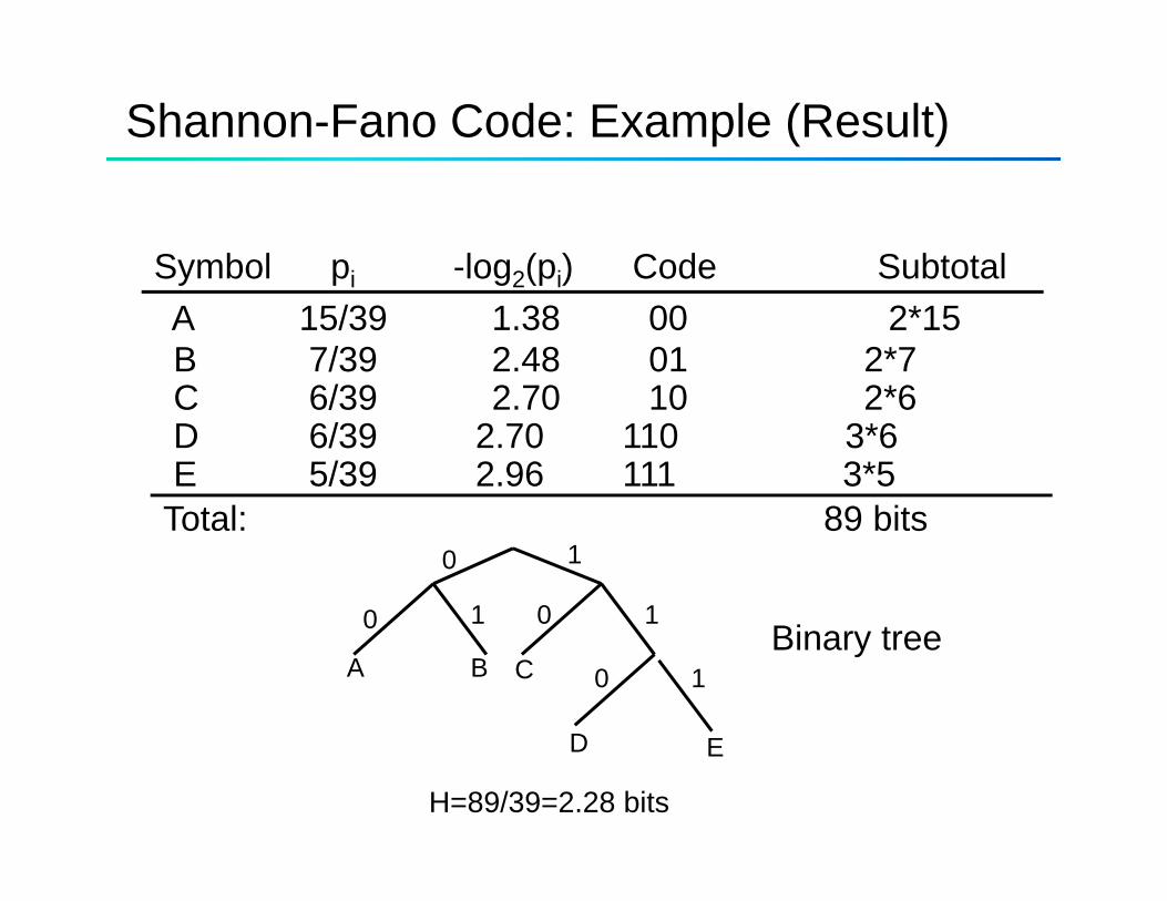
Shannon-Fano Code: Example (Result)
Symbol pi -log2(pi) Code Subtotal y pi g2(pi)A 15/39 1.38 00 2*15B 7/39 2.48 01 2*7C 6/39 2 70 10 2*6C 6/39 2.70 10 2*6D 6/39 2.70 110 3*6 E 5/39 2.96 111 3*5
T t l 89 bitTotal: 89 bits0 1
0 11 00 11 0
10A CB
D
Binary tree
D E
H=89/39=2.28 bits
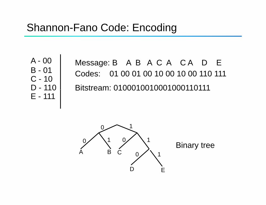
Shannon-Fano Code: Encoding
A - 00 Message: B A B A C A C A D EB - 01C - 10D - 110
Message: B A B A C A C A D ECodes: 01 00 01 00 10 00 10 00 110 111
Bitstream: 0100010010001000110111D 110E - 111
Bitstream: 0100010010001000110111
0 1
0 11 00 11 0
10A CB
D
Binary tree
D E
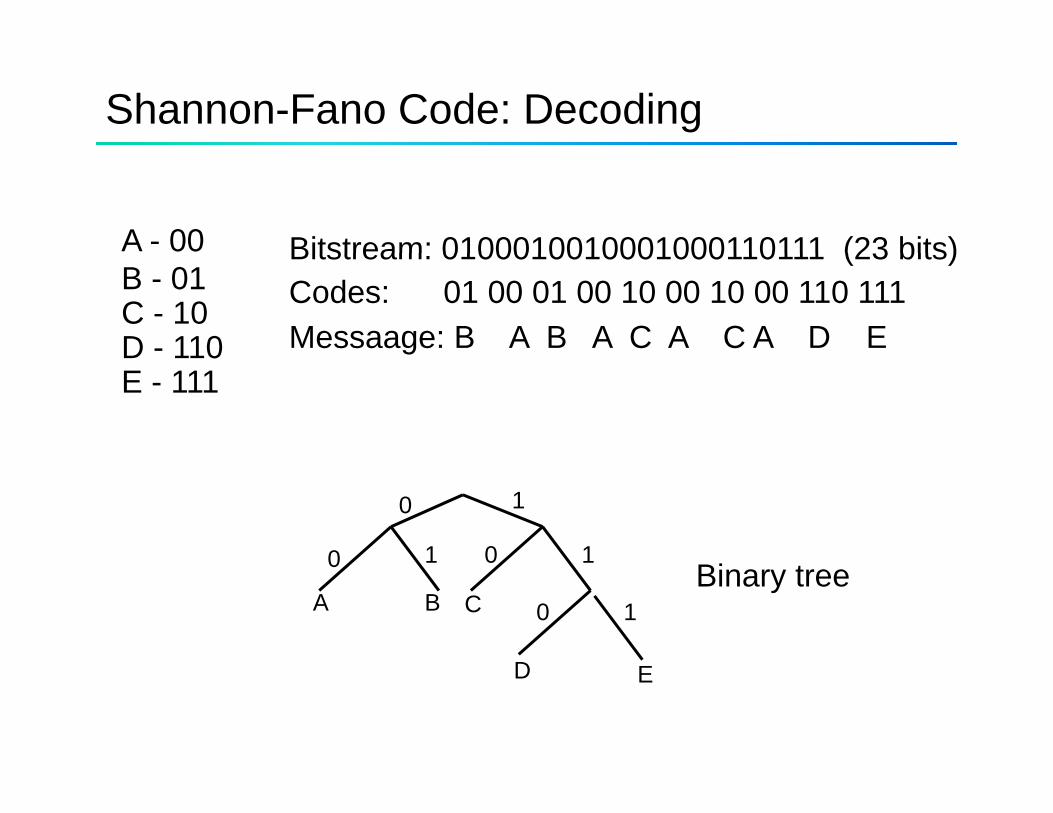
Shannon-Fano Code: Decoding
A - 00 Bitstream: 0100010010001000110111 (23 bits)B - 01C - 10D - 110
Bitstream: 0100010010001000110111 (23 bits)Codes: 01 00 01 00 10 00 10 00 110 111Messaage: B A B A C A C A D ED 110
E - 111
0 1
0 11 00 11 0
10A CB
D
Binary tree
D E
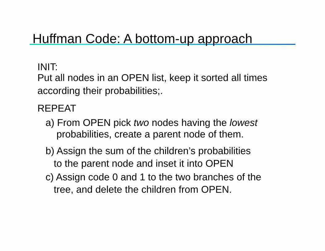
Huffman Code: A bottom-up approach
INIT:Put all nodes in an OPEN list keep it sorted all timesPut all nodes in an OPEN list, keep it sorted all timesaccording their probabilities;.
REPEATREPEATa) From OPEN pick two nodes having the lowest
probabilities, create a parent node of them.
b) Assign the sum of the children’s probabilities to the parent node and inset it into OPEN
c) Assign code 0 and 1 to the two branches of the tree, and delete the children from OPEN.
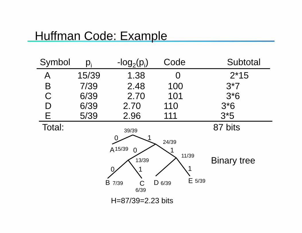
Huffman Code: Example
Symbol pi -log2(pi) Code Subtotal A 15/39 1 38 0 2*15A 15/39 1.38 0 2*15B 7/39 2.48 100 3*7C 6/39 2.70 101 3*6D 6/39 2.70 110 3*6 E 5/39 2.96 111 3*5
Total: 87 bits39/390 1
10ABinary tree11/39
15/39
13/39
24/39
39/39
10
C D E
1
B
Binary tree
6/39 5/39
6/397/39
13/39
H=87/39=2.23 bits6/39
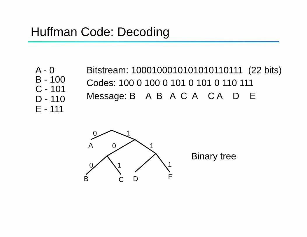
Huffman Code: Decoding
A - 0 Bitstream: 1000100010101010110111 (22 bits)B - 100 C - 101D - 110
( )Codes: 100 0 100 0 101 0 101 0 110 111Message: B A B A C A C A D E
E - 111
0 10 1
10
10
A
1Binary tree
10
C D E
1
B
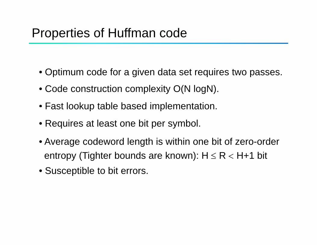
Properties of Huffman code
• Optimum code for a given data set requires two passes.p g q p
• Code construction complexity O(N logN).
• Fast lookup table based implementationFast lookup table based implementation.
• Requires at least one bit per symbol.
A d d l h i i hi bi f d• Average codeword length is within one bit of zero-order entropy (Tighter bounds are known): H ≤ R < H+1 bitSusceptible to bit errors• Susceptible to bit errors.
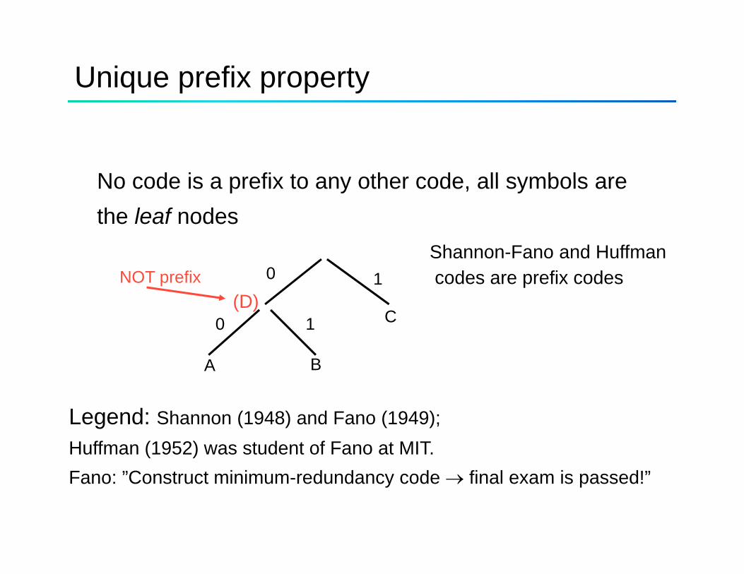
Unique prefix property
No code is a prefix to any other code all symbols areNo code is a prefix to any other code, all symbols are the leaf nodes
Shannon Fano and Huffman0
0
1
1 C
Shannon-Fano and Huffmancodes are prefix codes
(D)NOT prefix
0 1
A B
Legend: Shannon (1948) and Fano (1949); Huffman (1952) was student of Fano at MIT.Fano: ”Construct minimum-redundancy code → final exam is passed!”
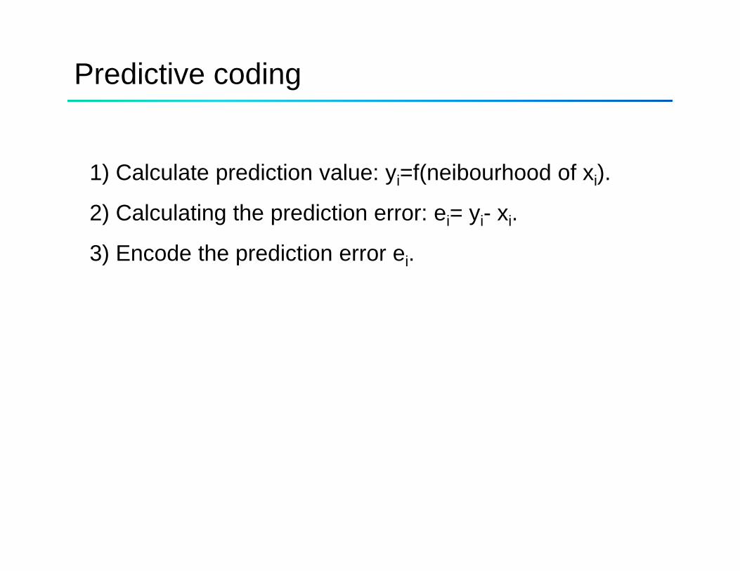
Predictive coding
1) Calculate prediction value: yi=f(neibourhood of xi)1) Calculate prediction value: yi f(neibourhood of xi).
2) Calculating the prediction error: ei= yi- xi.
3) Encode the prediction error e3) Encode the prediction error ei.
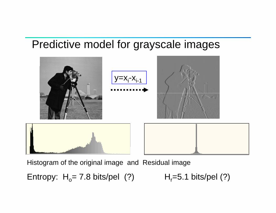
Predictive model for grayscale images
y=xi-xi-1
Histogram of the original image and Residual image
E t H 7 8 bit / l (?) H 5 1 bit / l (?)Entropy: Ho= 7.8 bits/pel (?) Hr=5.1 bits/pel (?)
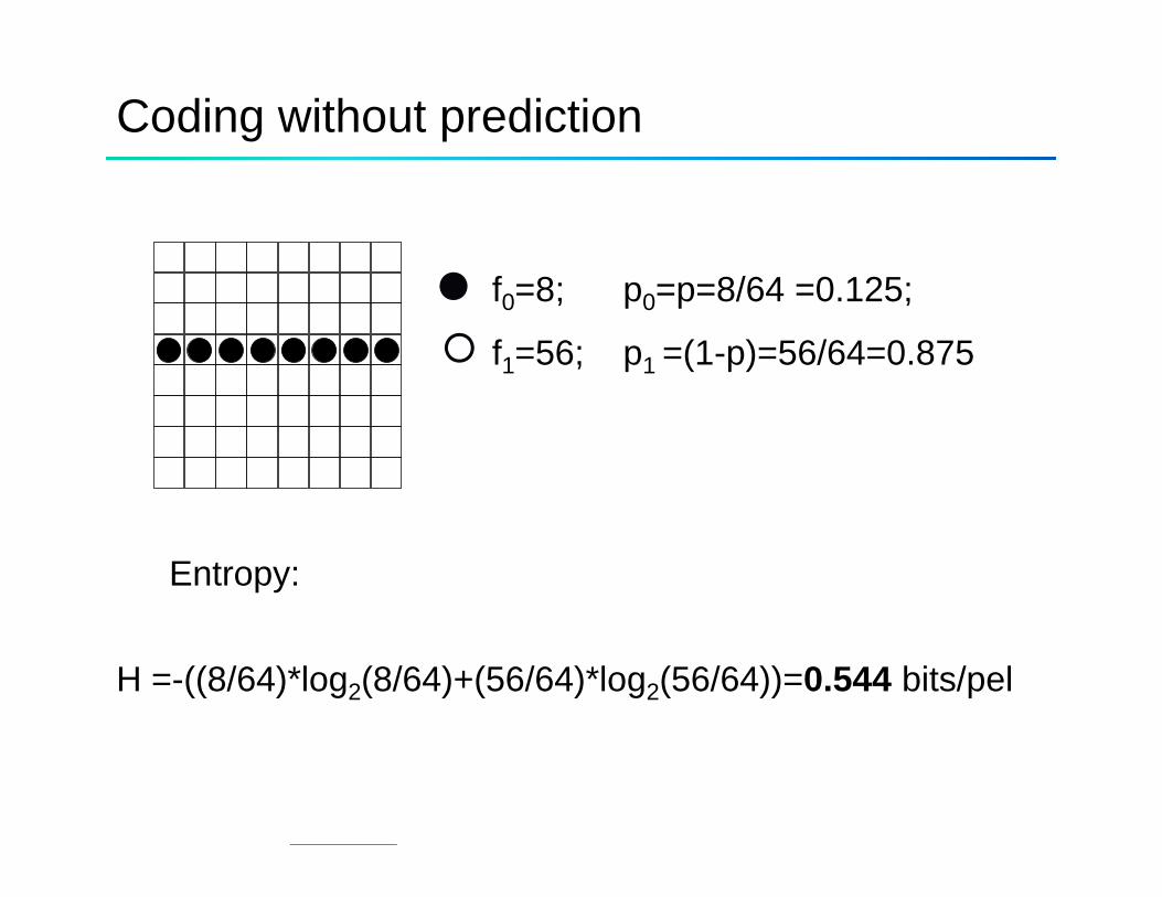
Coding without prediction
f 8 8/64 0 125f0=8; p0=p=8/64 =0.125;
f1=56; p1 =(1-p)=56/64=0.875
Entropy:
H =-((8/64)*log2(8/64)+(56/64)*log2(56/64))=0.544 bits/pel
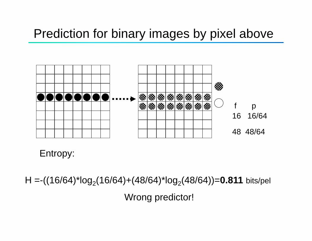
Prediction for binary images by pixel above
f pf p16 16/64
48 48/64
Entropy:
H =-((16/64)*log2(16/64)+(48/64)*log2(48/64))=0.811 bits/pel
Wrong predictor!Wrong predictor!
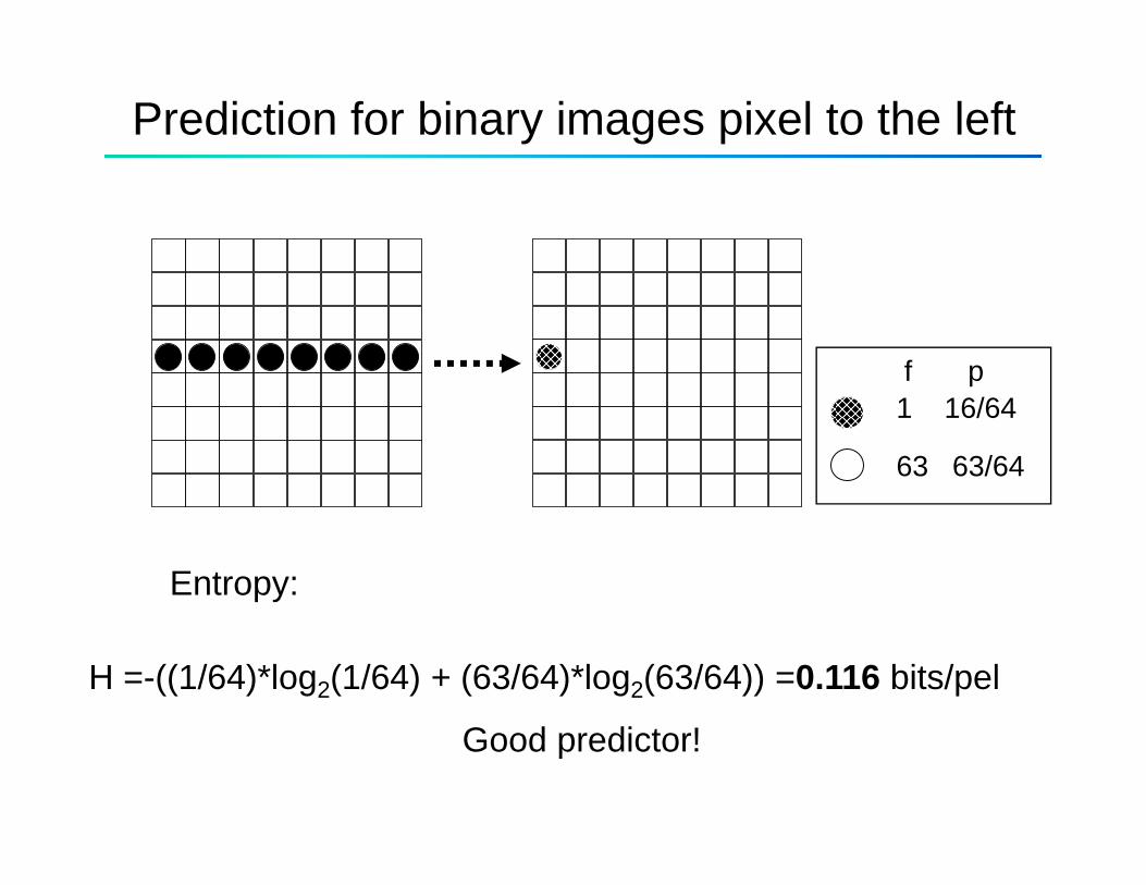
Prediction for binary images pixel to the left
f p1 16/64
63 63/64
Entropy:
H =-((1/64)*log2(1/64) + (63/64)*log2(63/64)) =0.116 bits/pel
Good predictor!
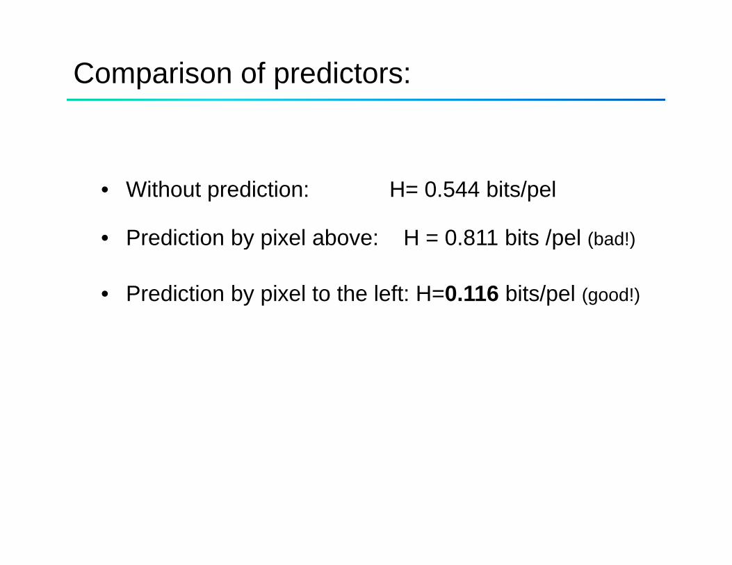
Comparison of predictors:
• Without prediction: H= 0.544 bits/pel
• Prediction by pixel above: H = 0.811 bits /pel (bad!)y p p ( )
• Prediction by pixel to the left: H=0.116 bits/pel (good!)
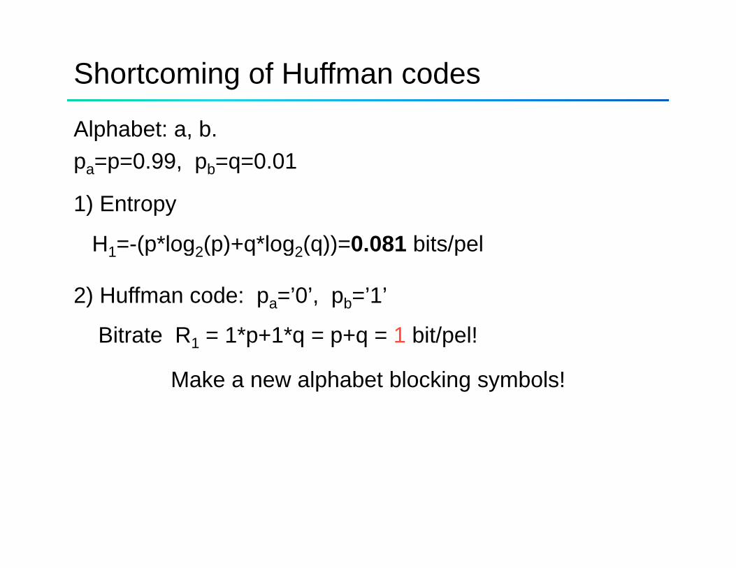
Shortcoming of Huffman codes
Alphabet: a, b.pa=p=0.99, pb=q=0.01
1) Entropy
H1=-(p*log2(p)+q*log2(q))=0.081 bits/pelH1 (p log2(p)+q log2(q)) 0.081 bits/pel
2) Huffman code: pa=’0’, pb=’1’
Bitrate R1 = 1*p+1*q = p+q = 1 bit/pel!
Make a new alphabet blocking symbols!g y
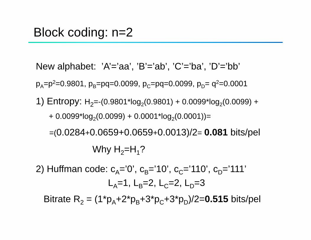
Block coding: n=2
New alphabet: ’A’=’aa’, ’B’=’ab’, ’C’=’ba’, ’D’=’bb’
pA=p2=0.9801, pB=pq=0.0099, pC=pq=0.0099, pD= q2=0.0001
1) Entropy: H2=-(0.9801*log2(0.9801) + 0.0099*log2(0.0099) +) py 2 ( g2( ) g2( )
+ 0.0099*log2(0.0099) + 0.0001*log2(0.0001))=
=(0.0284+0.0659+0.0659+0.0013)/2= 0.081 bits/pel(0.0284 0.0659 0.0659 0.0013)/2 0.081 bits/pel
Why H2=H1?
2) H ff d ’0’ ’10’ ’110’ ’111’2) Huffman code: cA=’0’, cB=’10’, cC=’110’, cD=’111’ LA=1, LB=2, LC=2, LD=3
Bit t R (1* 2* 3* 3* )/2 0 515 bit / lBitrate R2 = (1*pA+2*pB+3*pC+3*pD)/2=0.515 bits/pel
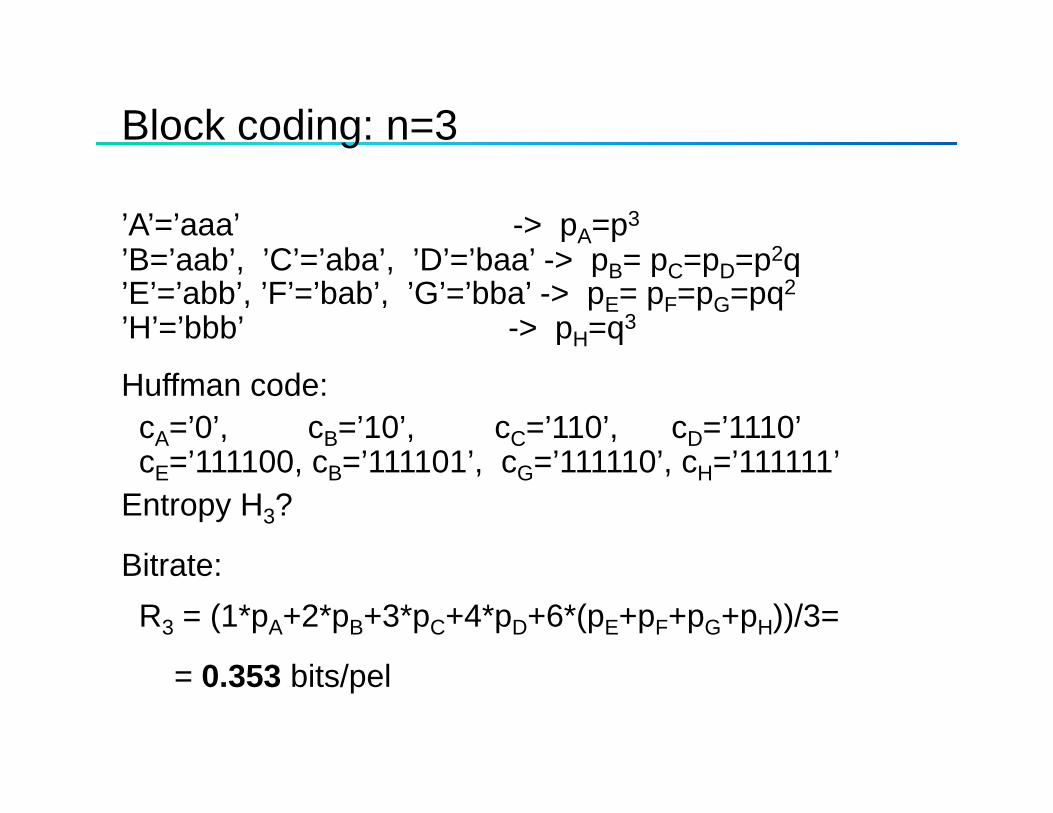
Block coding: n=3
’A’=’aaa’ -> pA=p3
’B ’ b’ ’C’ ’ b ’ ’D’ ’b ’ > 2’B=’aab’, ’C’=’aba’, ’D’=’baa’ -> pB= pC=pD=p2q’E’=’abb’, ’F’=’bab’, ’G’=’bba’ -> pE= pF=pG=pq2
’H’=’bbb’ -> pH=q3
Huffman code: cA=’0’, cB=’10’, cC=’110’, cD=’1110’ c =’111100 c =’111101’ c =’111110’ c =’111111’cE= 111100, cB= 111101 , cG= 111110 , cH= 111111
Entropy H3?
Bitrate:Bitrate: R3 = (1*pA+2*pB+3*pC+4*pD+6*(pE+pF+pG+pH))/3=
= 0.353 bits/pel
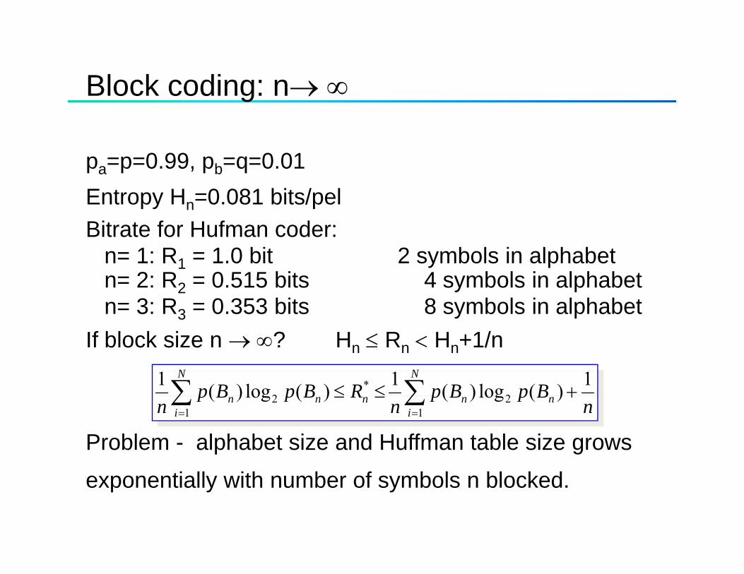
Block coding: n→ ∞
pa=p=0.99, pb=q=0.01Entropy Hn=0.081 bits/pel Bitrate for Hufman coder:
1 R 1 0 bit 2 b l i l h b tn= 1: R1 = 1.0 bit 2 symbols in alphabetn= 2: R2 = 0.515 bits 4 symbols in alphabetn= 3: R3 = 0.353 bits 8 symbols in alphabet
If block size n → ∞? Hn ≤ Rn < Hn+1/n
∑∑ +≤≤NN
BpBpRBpBp 2*
21)(log)(1)(log)(1
Problem - alphabet size and Huffman table size grows
∑∑==
+≤≤i
nni
nnn nBpBp
nRBpBp
n 12
12 )(log)()(log)(
exponentially with number of symbols n blocked.
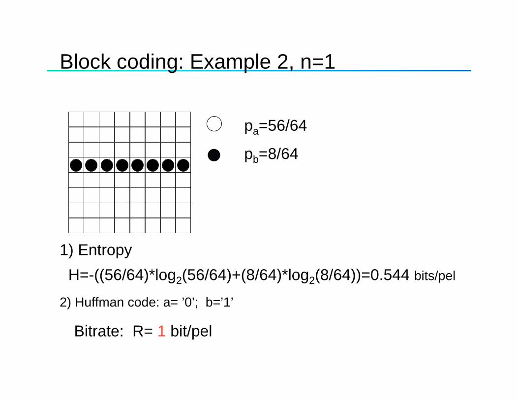
Block coding: Example 2, n=1
p =56/64pa=56/64
pb=8/64
1) Entropy H=-((56/64)*log (56/64)+(8/64)*log (8/64))=0 544 bits/pelH=-((56/64) log2(56/64)+(8/64) log2(8/64))=0.544 bits/pel
2) Huffman code: a= ’0’; b=’1’
Bit t R 1 bit/ lBitrate: R= 1 bit/pel
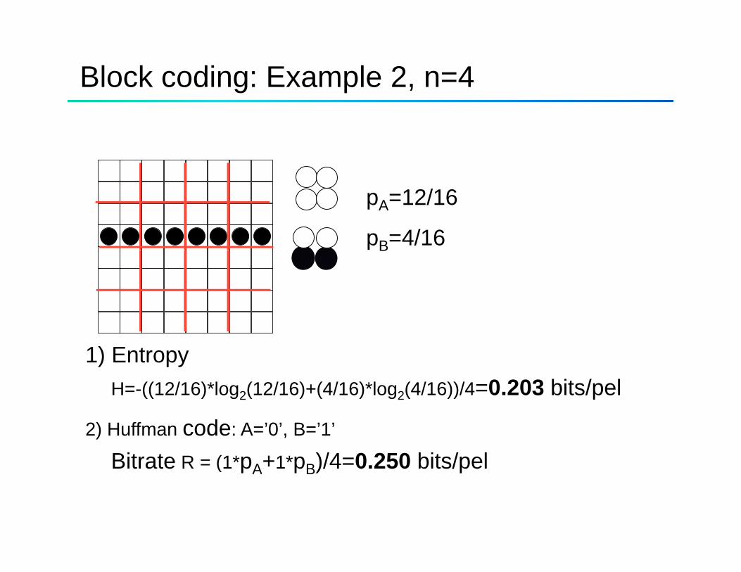
Block coding: Example 2, n=4
pA=12/16
pB=4/16B
1) Entropy H=-((12/16)*log2(12/16)+(4/16)*log2(4/16))/4=0.203 bits/pelH ((12/16) log2(12/16) (4/16) log2(4/16))/4 0.203 bits/pel
2) Huffman code: A=’0’, B=’1’
Bitrate R = (1*pA+1*pB)/4=0.250 bits/pelBitrate R (1 pA 1 pB)/4 0.250 bits/pel
Binary image compression• Run-length coding• Predictive coding• READ code• Block coding• G3 and G4• JBIG: Prepared by Joint Bi-Level Image Expert Group in
19921992
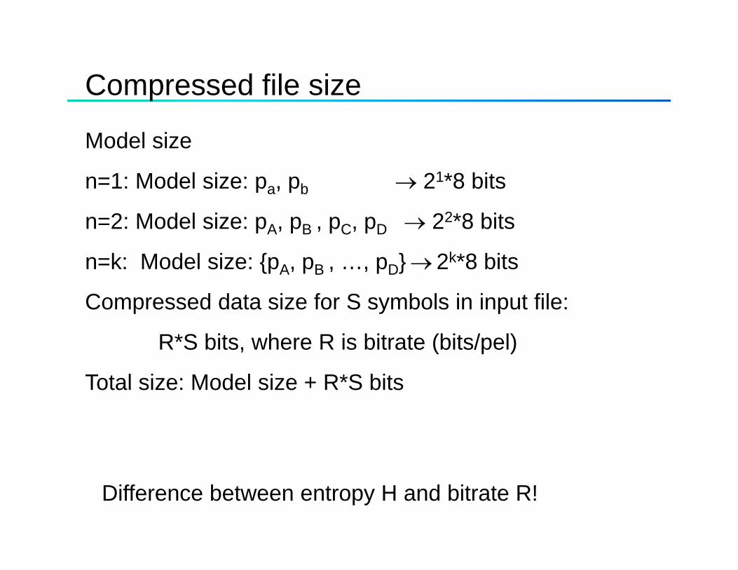
Compressed file size
Model size
n=1: Model size: p p 21*8 bitsn=1: Model size: pa, pb → 21*8 bits
n=2: Model size: pA, pB , pC, pD → 22*8 bits
n=k: Model size: {pA, pB , …, pD} → 2k*8 bits
Compressed data size for S symbols in input file:
R*S bits, where R is bitrate (bits/pel)
Total size: Model size + R*S bits
Difference between entropy H and bitrate R!
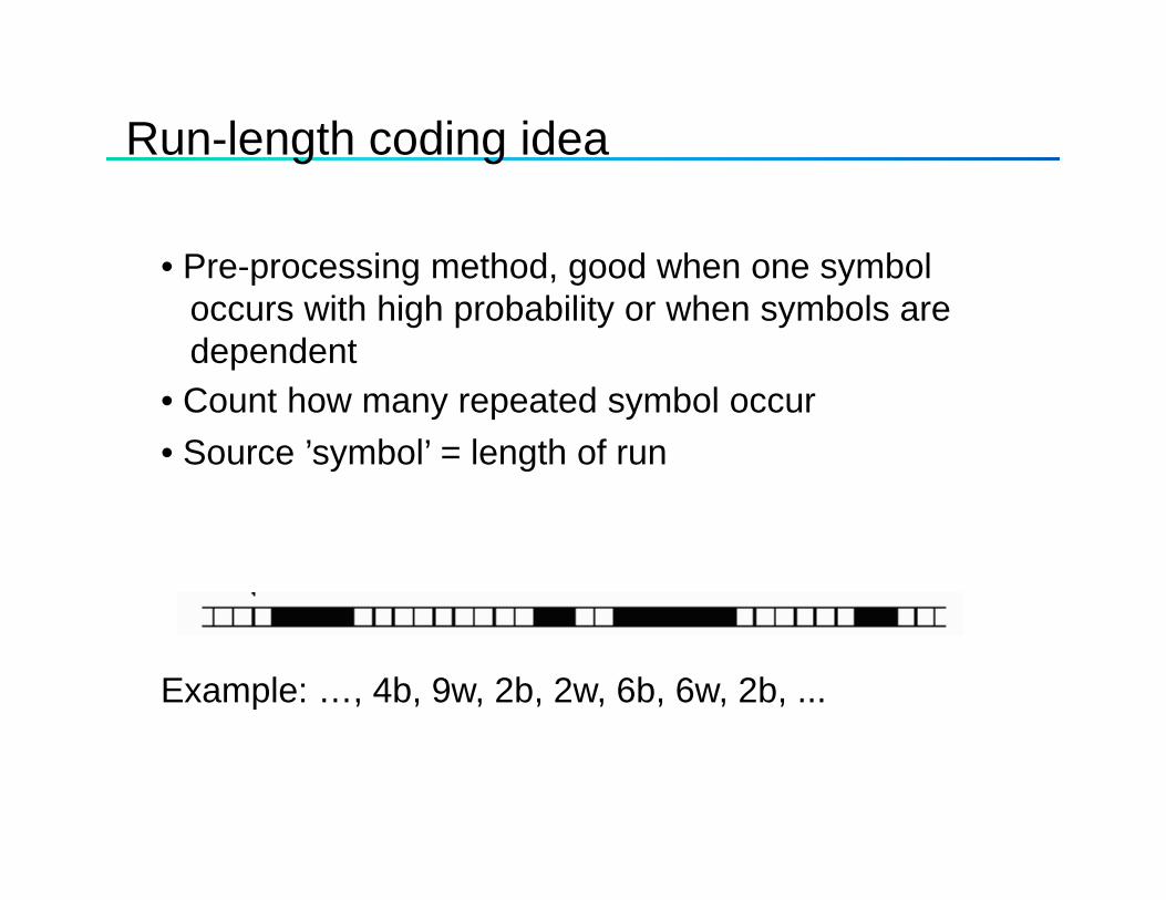
Run-length coding idea
• Pre-processing method, good when one symbol p g , g yoccurs with high probability or when symbols aredependentC t h t d b l• Count how many repeated symbol occur
• Source ’symbol’ = length of run
Example: …, 4b, 9w, 2b, 2w, 6b, 6w, 2b, ...
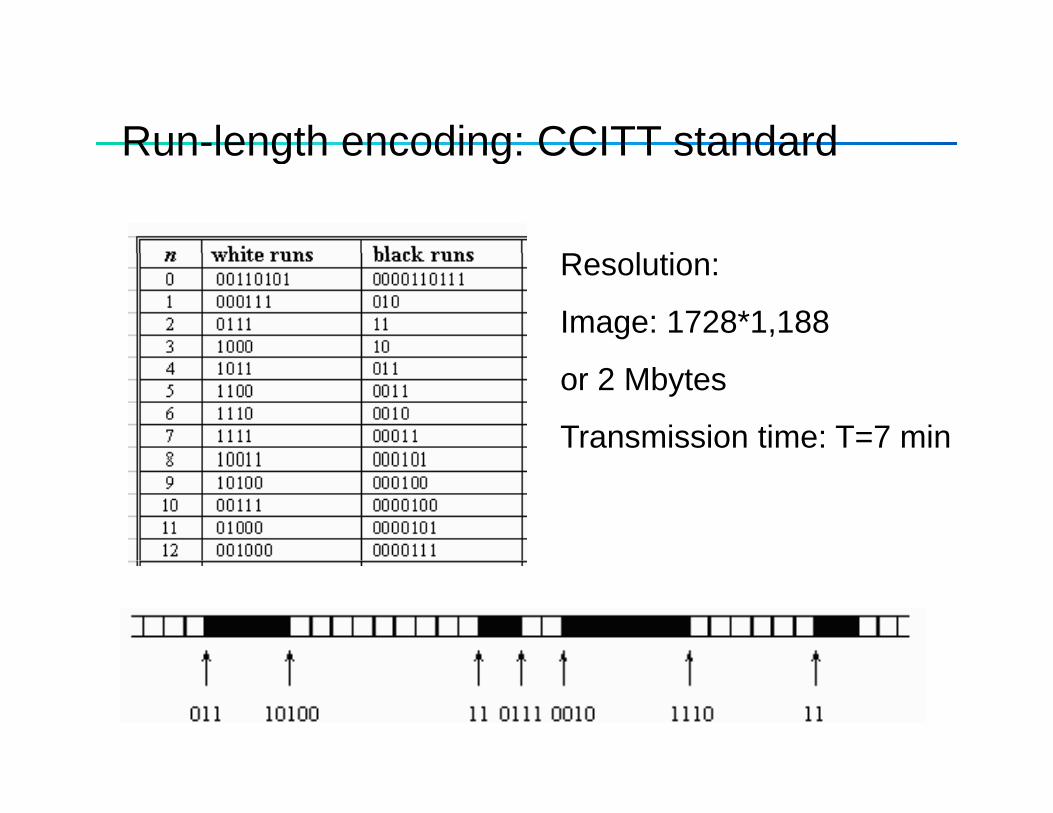
Run-length encoding: CCITT standardRun length encoding: CCITT standard
R l tiResolution:
Image: 1728*1,188
or 2 Mbytes
Transmission time: T=7 min
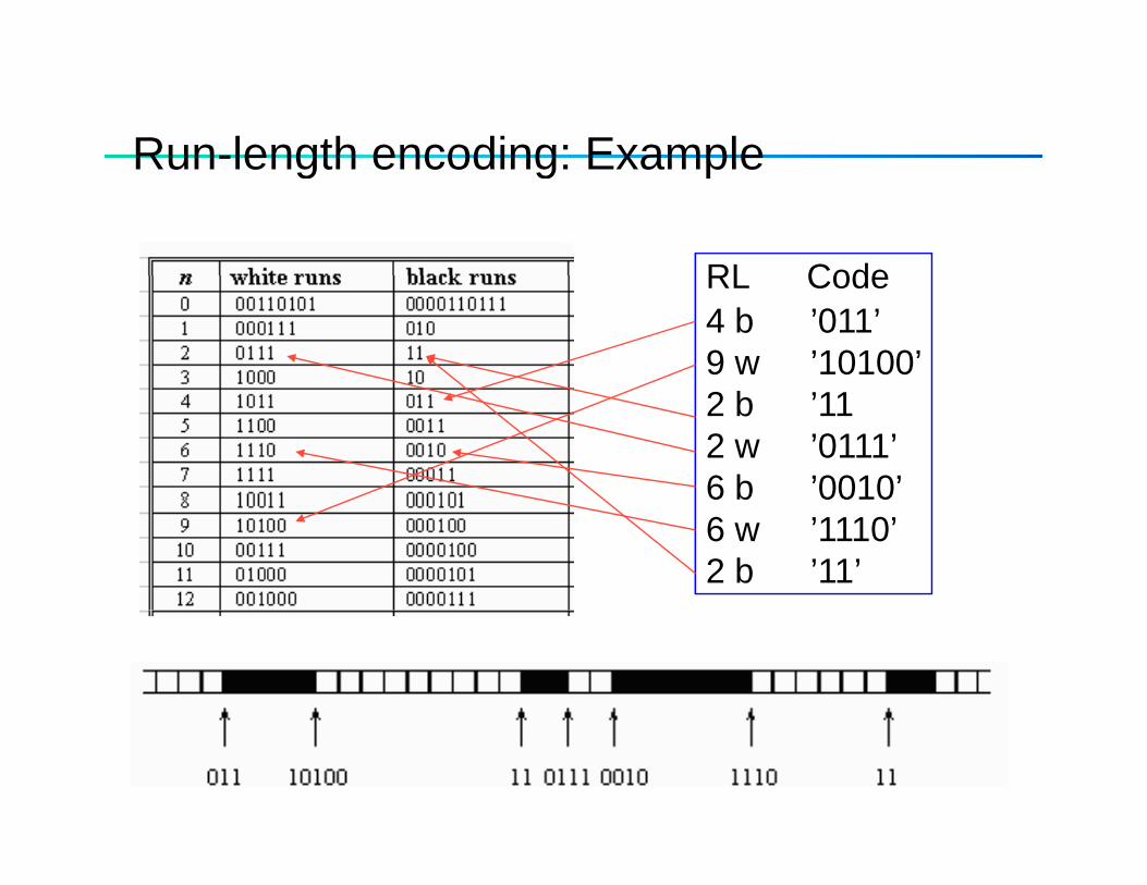
Run-length encoding: ExampleRun length encoding: Example
RL CodeRL Code4 b ’011’ 9 w ’10100’2 b ’112 w ’0111’6 b ’0010’6 b 00106 w ’1110’2 b ’11’
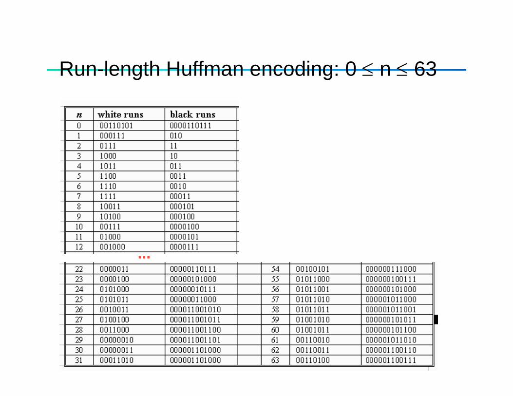
Run-length Huffman encoding: 0 ≤ n ≤ 63Run length Huffman encoding: 0 ≤ n ≤ 63
...
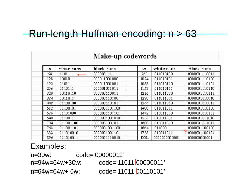
Run-length Huffman encoding: n > 63Run length Huffman encoding: n > 63
?
Examples: n=30w: code=’00000011’
?
n=94w=64w+30w: code=’11011 00000011’n=64w=64w+ 0w: code=’11011 00110101’
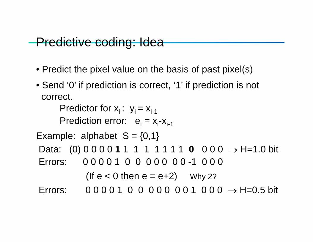
Predictive coding: IdeaPredictive coding: Idea
• Predict the pixel value on the basis of past pixel(s)
• Send ‘0’ if prediction is correct, ‘1’ if prediction is notcorrect.
P di t fPredictor for xi : yi = xi-1 Prediction error: ei = xi-xi-1
Example: alphabet S = {0 1}Example: alphabet S = {0,1} Data: (0) 0 0 0 0 1 1 1 1 1 1 1 1 0 0 0 0 → H=1.0 bitErrors: 0 0 0 0 1 0 0 0 0 0 0 0 -1 0 0 0
(If e < 0 then e = e+2) Why 2?
Errors: 0 0 0 0 1 0 0 0 0 0 0 0 1 0 0 0 → H=0.5 bit
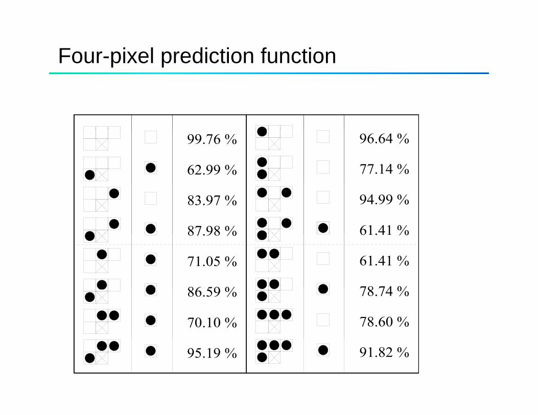
Four-pixel prediction function
62.99 %
96.64 %
77.14 %
99.76 %
83.97 %
87 98 %
94.99 %
61.41 %87.98 %
71.05 %
61.41 %
61.41 %
86.59 %
70.10 %
78.74 %
78.60 %
95.19 % 91.82 %
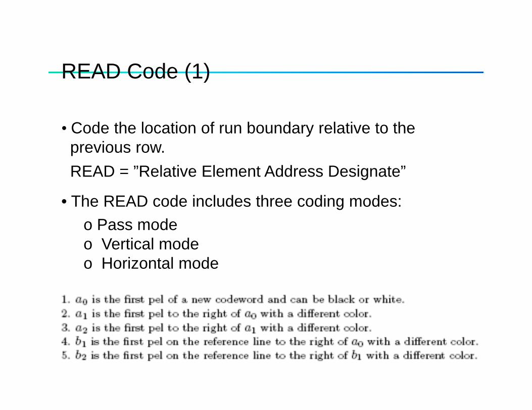
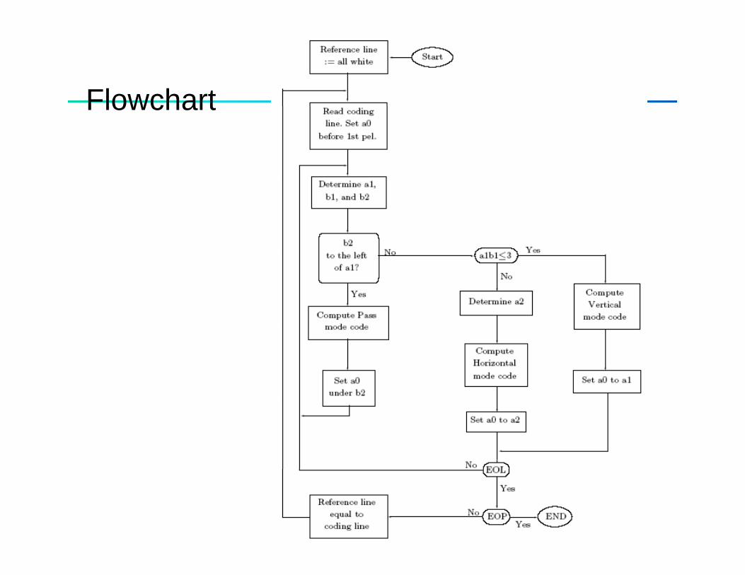
READ Code (1)READ Code (1)
• Code the location of run boundary relative to the• Code the location of run boundary relative to theprevious row.READ = ”Relative Element Address Designate”g
• The READ code includes three coding modes:o Pass modeo Vertical modeo Horizontal mode
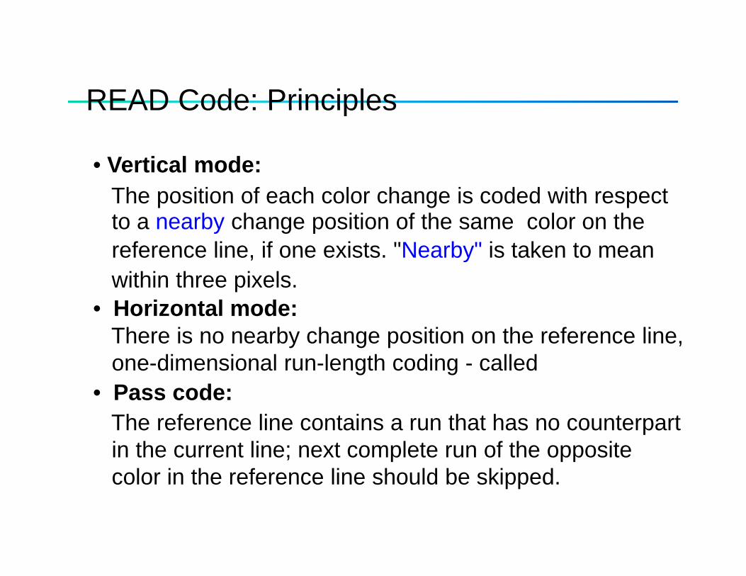
READ Code: PrinciplesREAD Code: Principles
• Vertical mode: The position of each color change is coded with respect to a nearby change position of the same color on the reference line if one exists "Nearby" is taken to meanreference line, if one exists. Nearby is taken to mean within three pixels.
• Horizontal mode:There is no nearby change position on the reference line,one-dimensional run-length coding - called
• Pass code:Pass code: The reference line contains a run that has no counterpartin the current line; next complete run of the opposite
l i th f li h ld b ki dcolor in the reference line should be skipped.
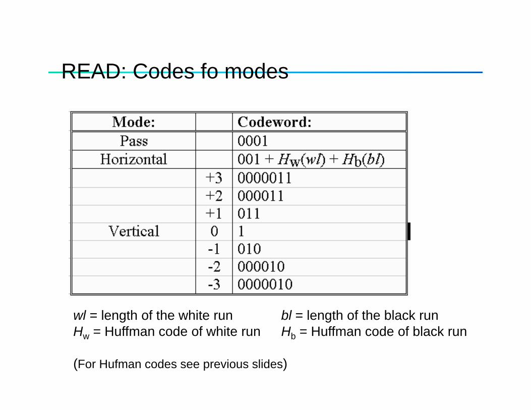
READ: Codes fo modesREAD: Codes fo modes
wl = length of the white run bl = length of the black runH = Huffman code of white run Hb = Huffman code of black runHw Huffman code of white run Hb Huffman code of black run
(For Hufman codes see previous slides)
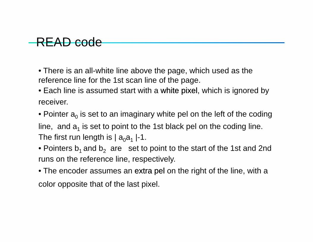
READ codeREAD code
• There is an all-white line above the page, which used as the reference line for the 1st scan line of the page.• Each line is assumed start with a white pixelwhite pixel, which is ignored by receiver. • Pointer a0 is set to an imaginary white pel on the left of the coding line, and a1 is set to point to the 1st black pel on the coding line. The first run length is | a a | 1The first run length is | a0a1 |-1. • Pointers b1 and b2 are set to point to the start of the 1st and 2ndruns on the reference line, respectively.• The encoder assumes an extra pelextra pel on the right of the line, with a
color opposite that of the last pixel.
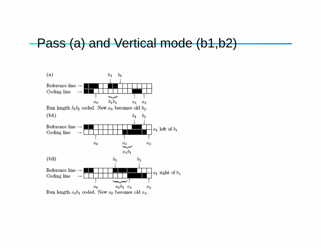
Pass (a) and Vertical mode (b1 b2)Pass (a) and Vertical mode (b1,b2)
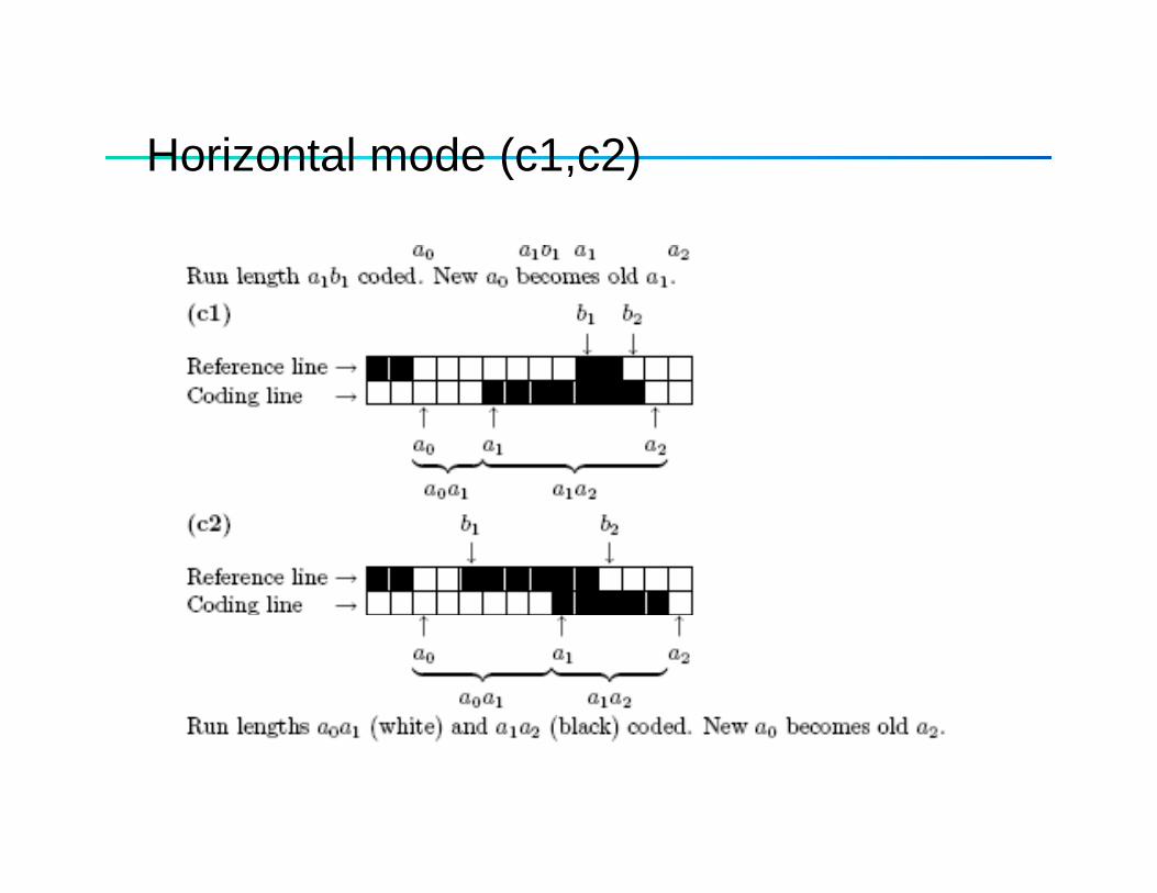
Horizontal mode (c1 c2)Horizontal mode (c1,c2)
FlowchartFlowchart
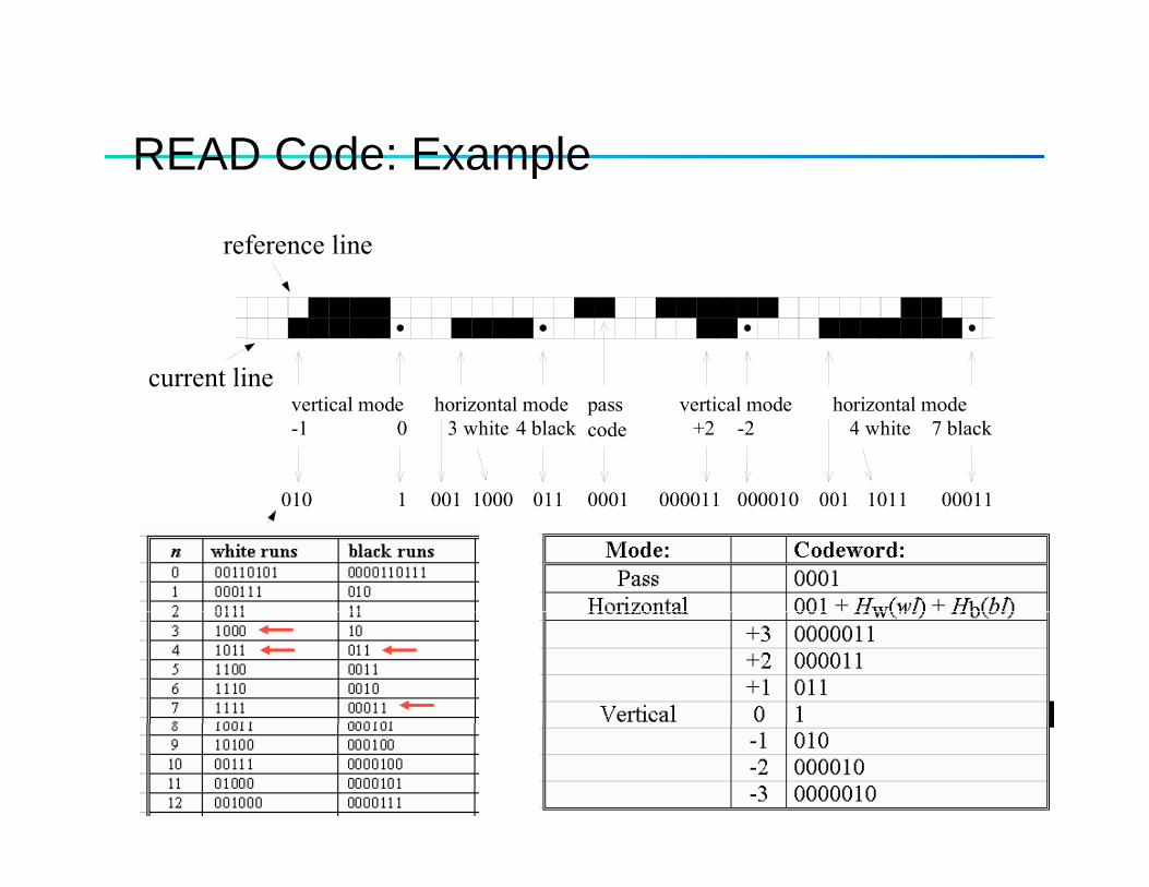
READ Code: ExampleREAD Code: Example
reference line
current linevertical mode
010
horizontal mode passcode
vertical mode horizontal mode-1 0 3 white 4 black +2 4 white 7 black-2
1 1000 011 0001 000011 000010 00011001001 1011010
code generated
1 1000 011 0001 000011 000010 00011001001 1011
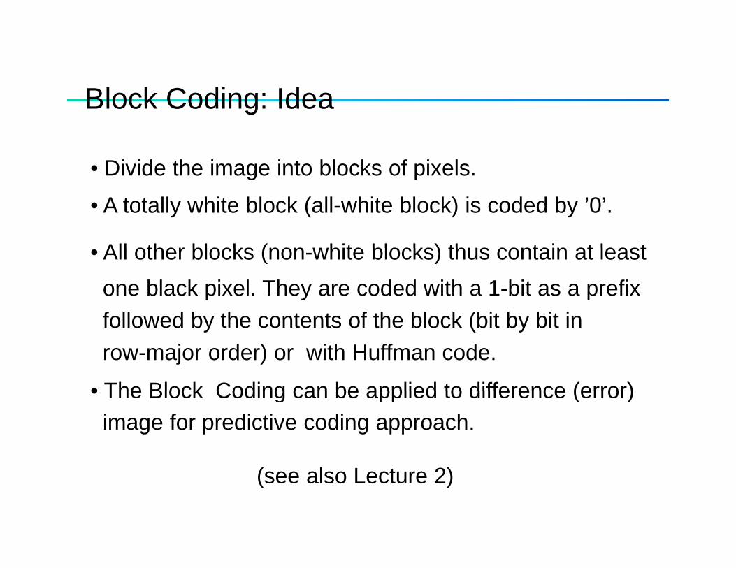
Block Coding: IdeaBlock Coding: Idea
• Divide the image into blocks of pixels. g p
• A totally white block (all-white block) is coded by ’0’.
All other blocks (non white blocks) thus contain at least• All other blocks (non-white blocks) thus contain at least one black pixel. They are coded with a 1-bit as a prefix followed by the contents of the block (bit by bit infollowed by the contents of the block (bit by bit in row-major order) or with Huffman code.
• The Block Coding can be applied to difference (error)• The Block Coding can be applied to difference (error) image for predictive coding approach.
(see also Lecture 2)
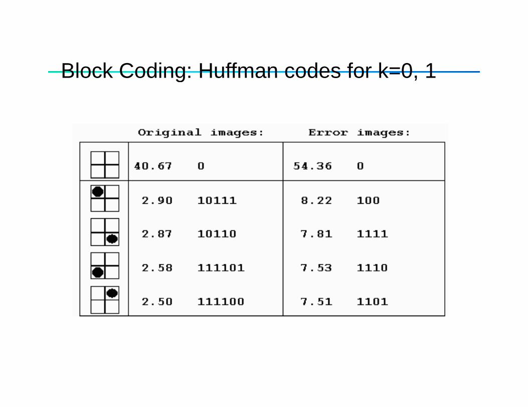
Block Coding: Huffman codes for k=0 1Block Coding: Huffman codes for k 0, 1
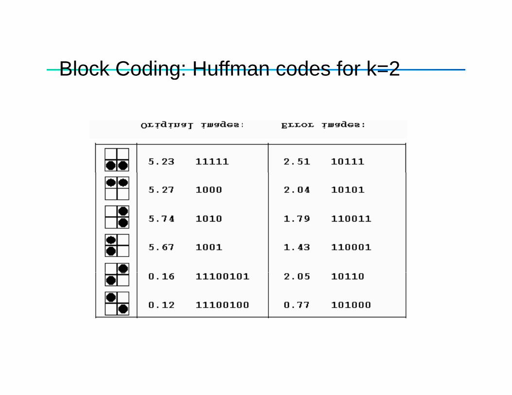
Block Coding: Huffman codes for k=2Block Coding: Huffman codes for k 2
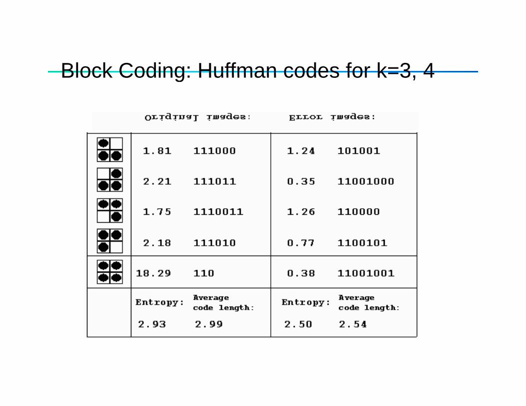
Block Coding: Huffman codes for k=3 4Block Coding: Huffman codes for k 3, 4
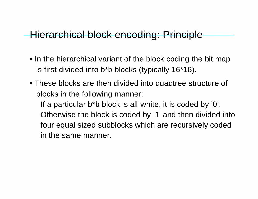
Hierarchical block encoding: PrincipleHierarchical block encoding: Principle
• In the hierarchical variant of the block coding the bit map g pis first divided into b*b blocks (typically 16*16).
• These blocks are then divided into quadtree structure ofqblocks in the following manner: If a particular b*b block is all-white, it is coded by ’0’.Oth i th bl k i d d b ’1’ d th di id d i tOtherwise the block is coded by ’1’ and then divided into four equal sized subblocks which are recursively coded in the same manner.in the same manner.
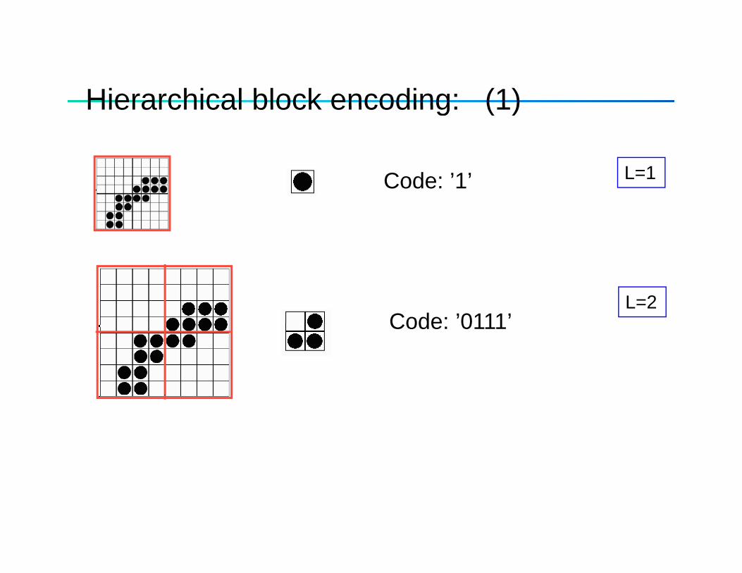
Hierarchical block encoding: (1)Hierarchical block encoding: (1)
Code: ’1’ L=1Code: 1 L 1
Code: ’0111’L=2
Code: 0111
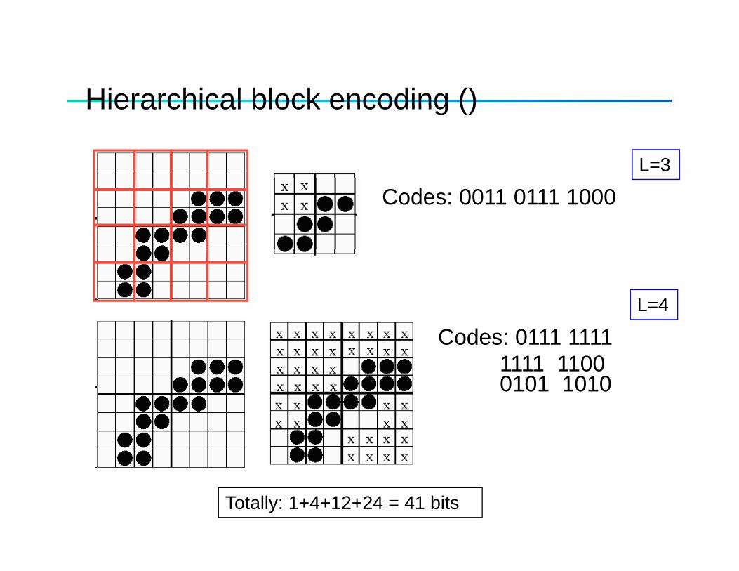
Hierarchical block encoding ()Hierarchical block encoding ()
L=3
Codes: 0011 0111 1000
L=4
Codes: 0111 1111 1111 11000101 1010
Totally: 1+4+12+24 = 41 bits

Hierarchical block encoding: ExampleHierarchical block encoding: Example
Image to be compressed: Code bits:1 0111 0011 0111 1000 0111 1111 11111 0111 0011 0111 1000
x xx x
0111 1111 11110101 1010 1100
x x x xx x x x
x xx x
x xx x
x x x xx x x xx xx x
x x
x xx xx x1 x x
x xx xx x
1
0 1 1 11
0 0 1 1 0 1 1 1 1 0 0 01+4+12+24=41
0111 1111 1111 0101 1010 1100
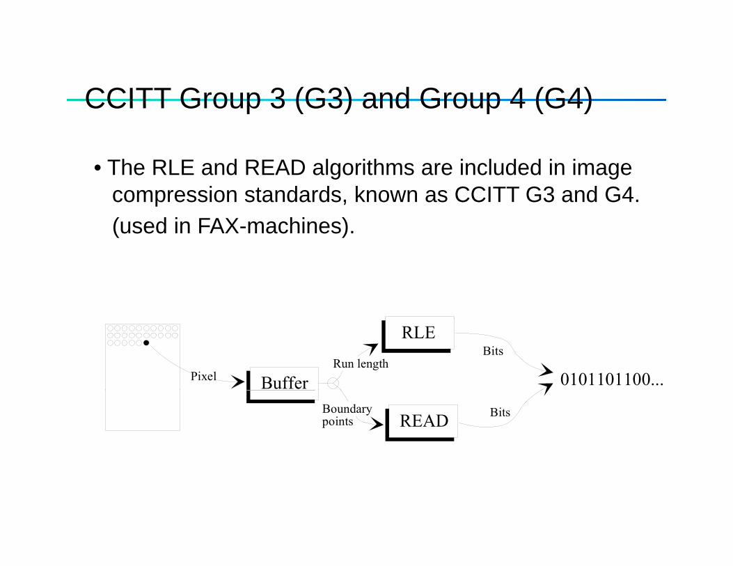
CCITT Group 3 (G3) and Group 4 (G4)CCITT Group 3 (G3) and Group 4 (G4)
• The RLE and READ algorithms are included in imageg gcompression standards, known as CCITT G3 and G4.(used in FAX-machines).
Buffer
RLE
0101101100...Run length
Bits
Pixel
READBoundary Bitspoints
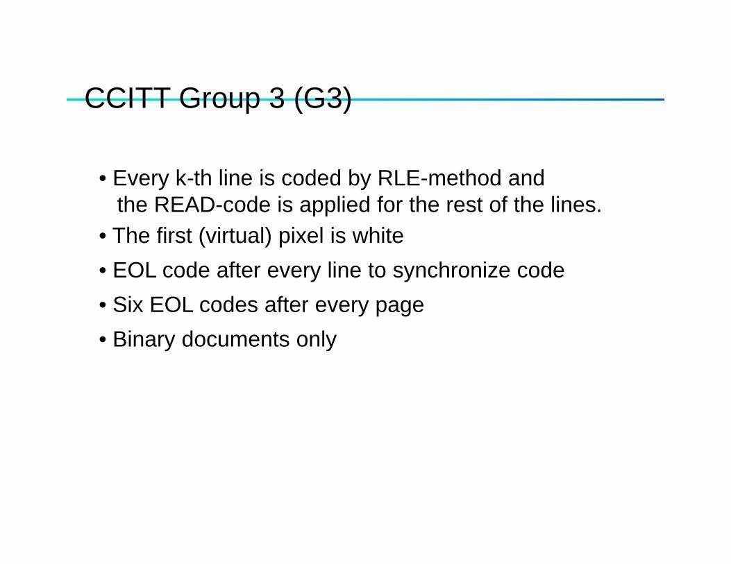
CCITT Group 3 (G3)CCITT Group 3 (G3)
• Every k th line is coded by RLE method and• Every k-th line is coded by RLE-method and the READ-code is applied for the rest of the lines.
• The first (virtual) pixel is white( ) p• EOL code after every line to synchronize code• Six EOL codes after every page• Binary documents only
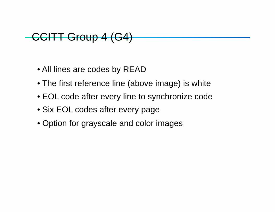
CCITT Group 4 (G4)CCITT Group 4 (G4)
• All lines are codes by READ
• The first reference line (above image) is white• EOL code after every line to synchronize code• Six EOL codes after every page• Option for grayscale and color images
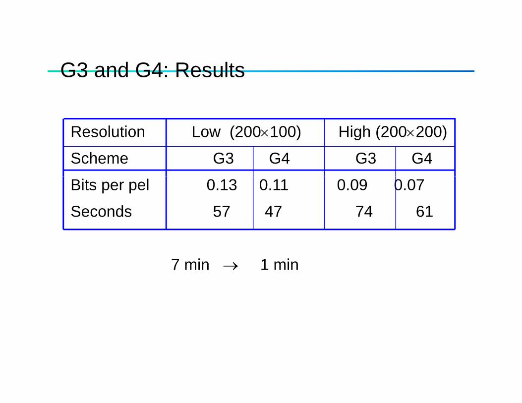
G3 and G4: ResultsG3 and G4: Results
Resolution Low (200×100) High (200×200)
Scheme G3 G4 G3 G4
Bits per pel 0.13 0.11 0.09 0.07
Seconds 57 47 74 61
7 min → 1 min
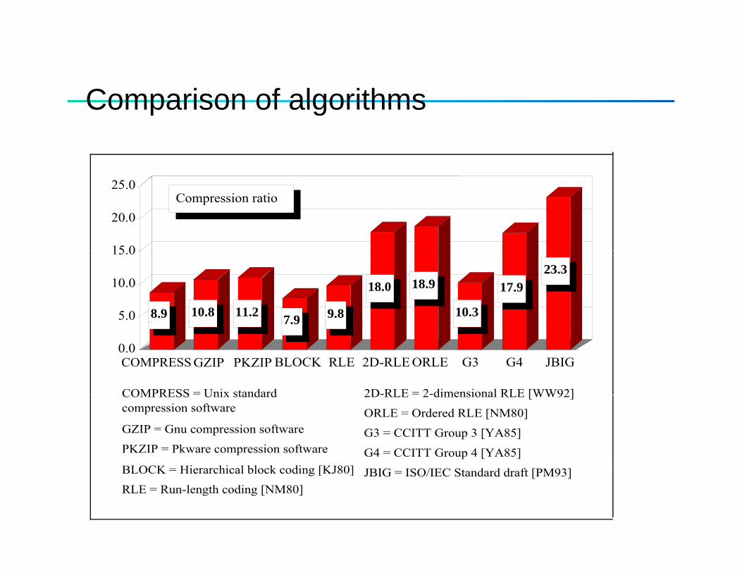
Comparison of algorithmsComparison of algorithms
15 0
20.0
25.0Compression ratio
5.0
10.0
15.0
7.9 9.8
18.0 18.9 17.923.3
10.38.9 10.8 11.2
BLOCK RLE 2D-RLE ORLE G3 G4 JBIG0.0
7.9
PKZIPGZIPCOMPRESS
COMPRESS = Unix standard 2D-RLE = 2-dimensional RLE [WW92]COMPRESS Unix standard compression software
GZIP = Gnu compression software
PKZIP = Pkware compression software
BLOCK Hi hi l bl k di [KJ80]
2D RLE 2 dimensional RLE [WW92]
ORLE = Ordered RLE [NM80]
G3 = CCITT Group 3 [YA85]
G4 = CCITT Group 4 [YA85]BLOCK = Hierarchical block coding [KJ80]
RLE = Run-length coding [NM80]JBIG = ISO/IEC Standard draft [PM93]
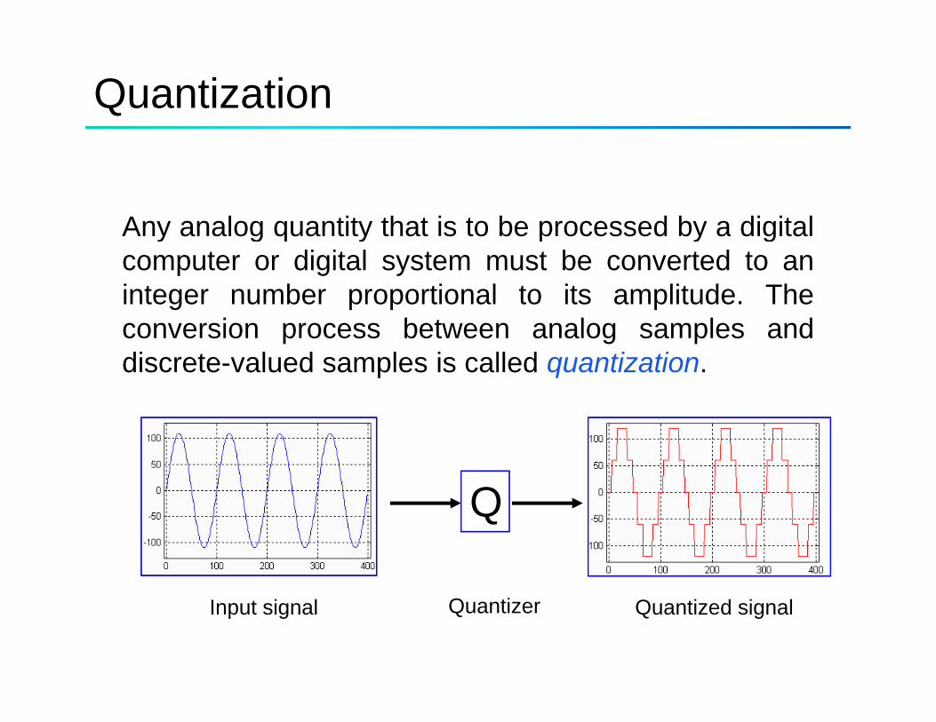
Quantization
Any analog quantity that is to be processed by a digitalAny analog quantity that is to be processed by a digitalcomputer or digital system must be converted to aninteger number proportional to its amplitude. Theconversion process between analog samples anddiscrete-valued samples is called quantization.
Input signal Quantized signalQuantizer
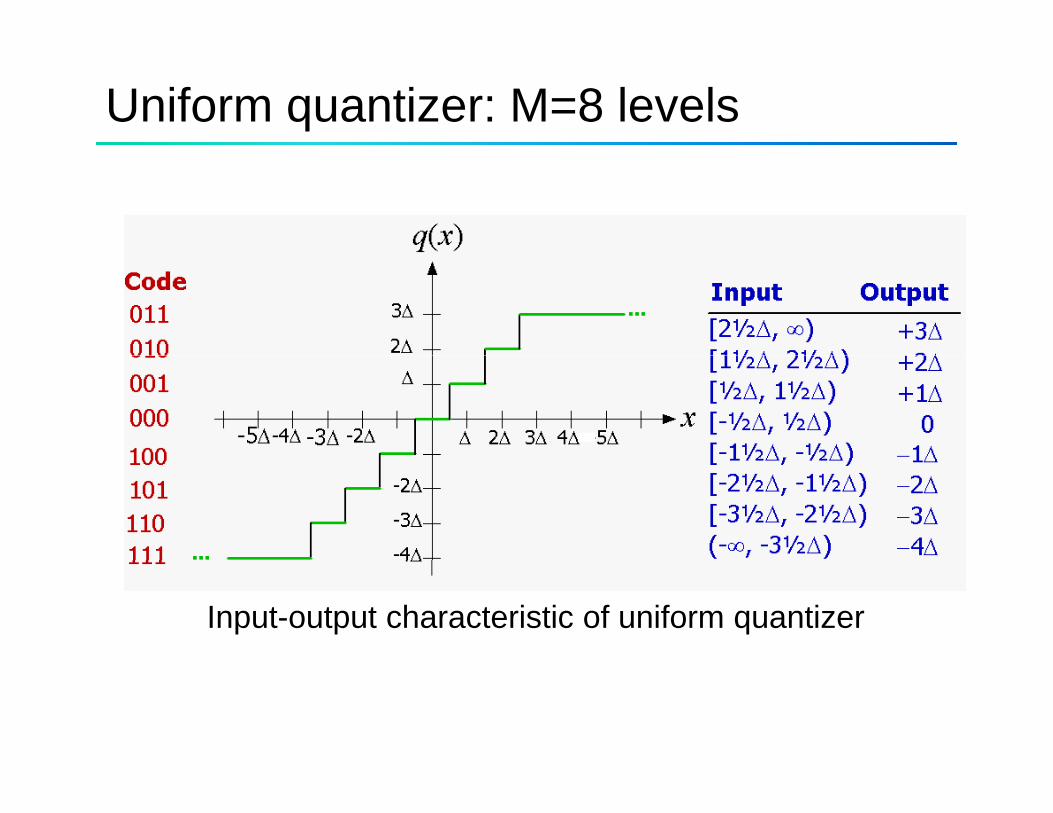
Uniform quantizer: M=8 levels
Input-output characteristic of uniform quantizer
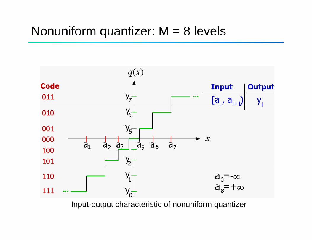
Nonuniform quantizer: M = 8 levels
Input-output characteristic of nonuniform quantizer

Nonuniform quantizer: M = 8 levels
Input-output characteristic of nonuniform quantizer
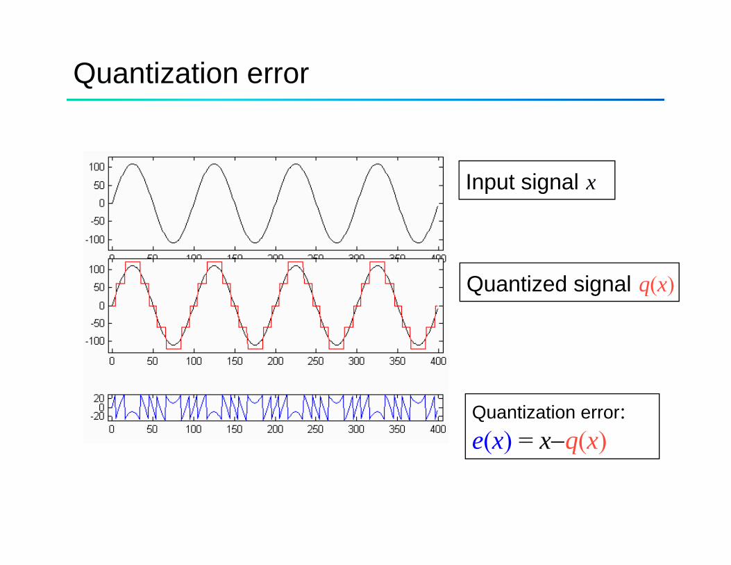
Quantization error
I t i lInput signal x
Quantized signal q(x)
Quantization error:e(x) = x−q(x)
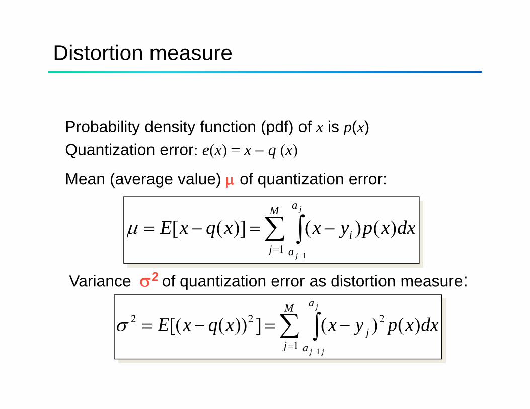
Distortion measure
Probability density function (pdf) of x is p(x)Probability density function (pdf) of x is p(x)Quantization error: e(x) = x − q (x)
Mean (average value) μ of quantization error:Mean (average value) μ of quantization error:
dxxpyxxqxEM a j
)()()]([ ∑ ∫ −=−=μ dxxpyxxqxEj a
i
j
)()()]([1
1
∑ ∫=
−
==μ
Variance σ2 of quantization error as distortion measure:Variance σ of quantization error as distortion measure:
dxxpyxxqxEM a
j
j
)()(]))([( 222 ∑ ∫ −=−=σ pyqj a
j
jj
)()(]))([(1
1
∑ ∫=
−
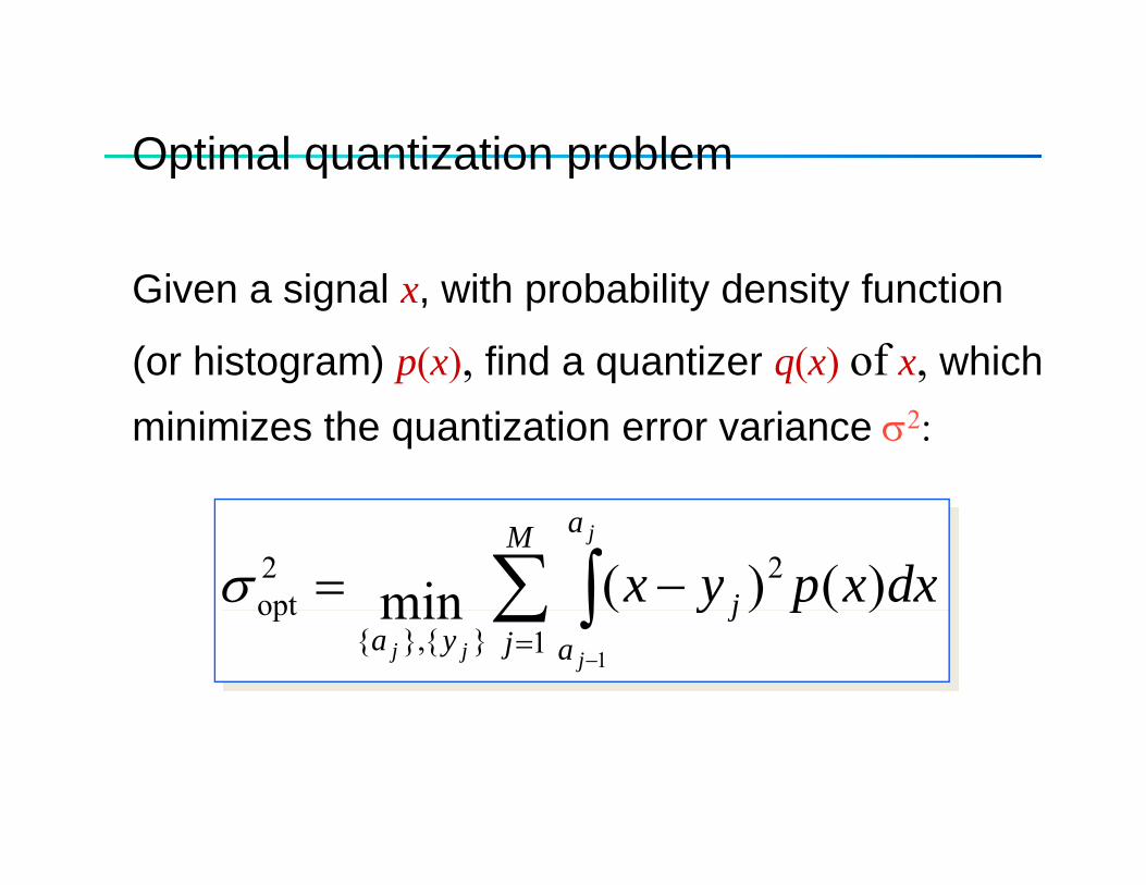
Optimal quantization problemOptimal quantization problem
Gi i l ith b bilit d it f tiGiven a signal x, with probability density function
(or histogram) p(x), find a quantizer q(x) of x, which minimizes the quantization error variance σ2:
dxxpyxM a
j
j
)()(min22
opt ∑ ∫ −=σ pyj a
jya
jjj
)()(min1}{},{
opt
1
∑ ∫=
−
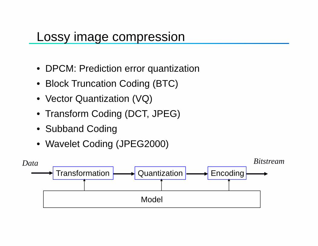
Lossy image compression
• DPCM: Prediction error quantization• Block Truncation Coding (BTC)• Vector Quantization (VQ)• Transform Coding (DCT, JPEG)• Subband Coding• Wavelet Coding (JPEG2000)
Data Bitstream
Model
Transformation Quantization Encoding
Model
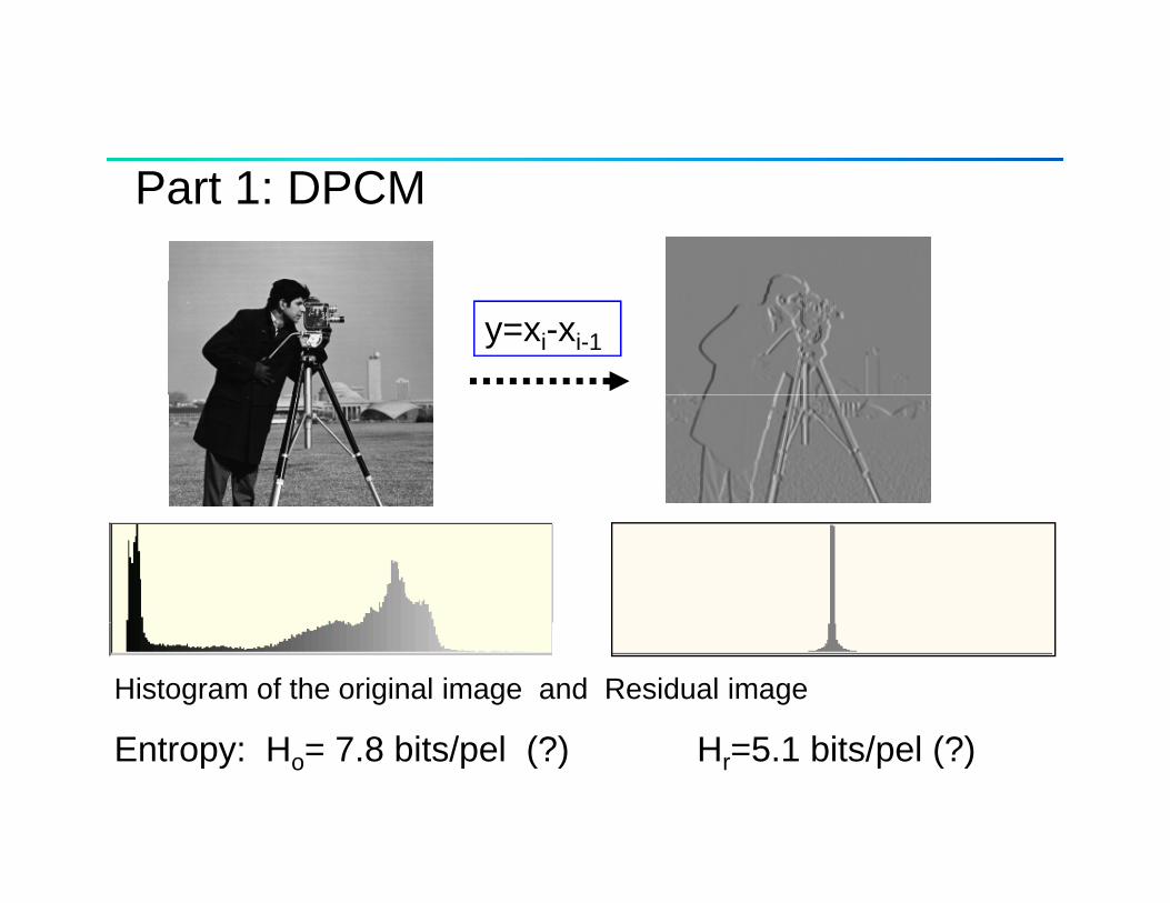
Part 1: DPCM
y=xi-xi-1
Histogram of the original image and Residual image
E t H 7 8 bit / l (?) H 5 1 bit / l (?)Entropy: Ho= 7.8 bits/pel (?) Hr=5.1 bits/pel (?)
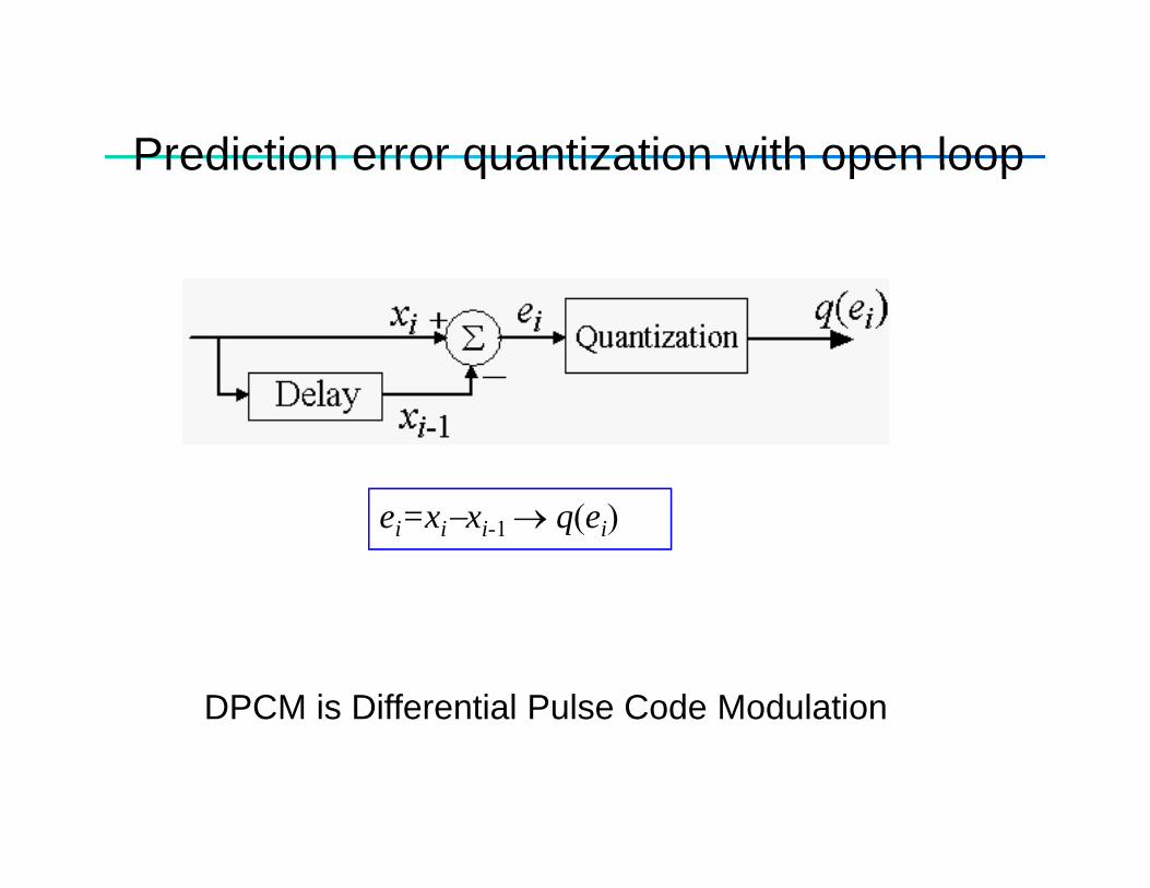
Prediction error quantization with open loopPrediction error quantization with open loop
ei=xi−xi-1 → q(ei)
DPCM is Differential Pulse Code Modulation
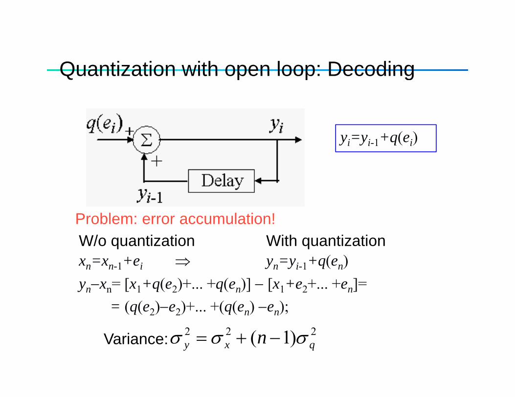
Quantization with open loop: DecodingQuantization with open loop: Decoding
yi=yi-1+q(ei)
Problem: error accumulation!Problem: error accumulation!W/o quantization With quantizationxn=xn-1+ei ⇒ yn=yi-1+q(en)yn−xn= [x1+q(e2)+... +q(en)] − [x1+e2+... +en]=
= (q(e2)−e2)+... +(q(en) −en);222 )1( qxy n σσσ −+=Variance:
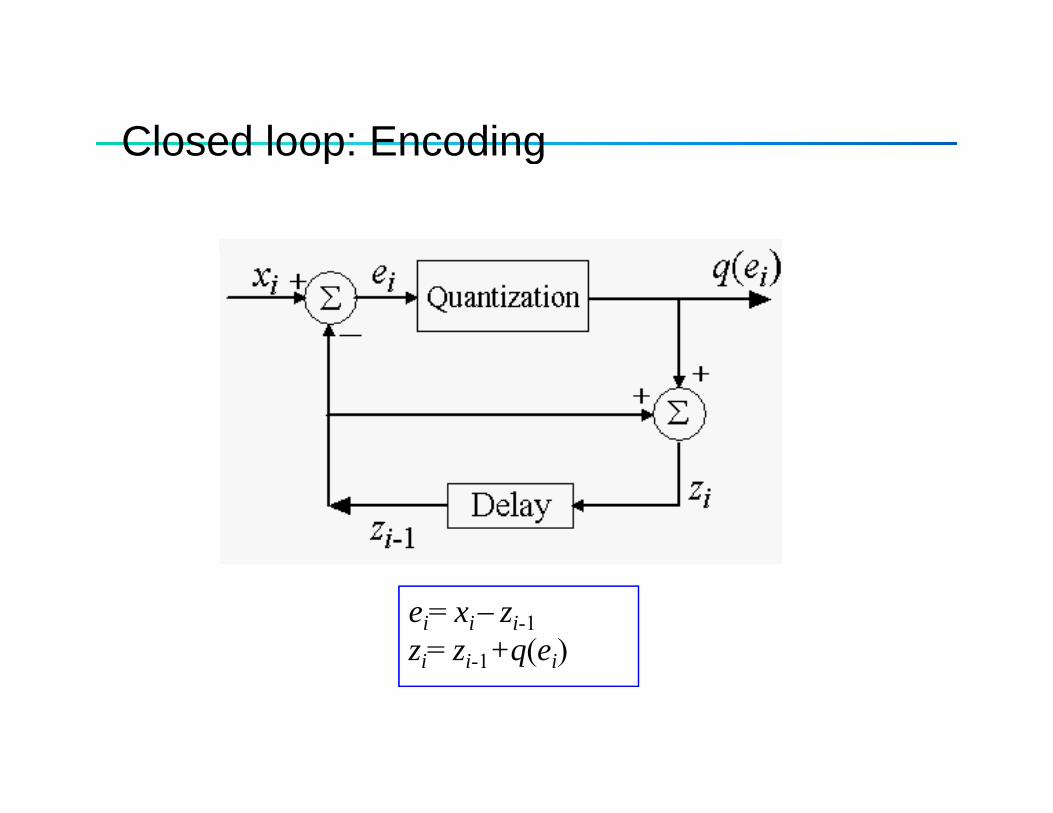
Closed loop: EncodingClosed loop: Encoding
ei=xi−xi-1 → q(ei)
ei= xi− zi-1zi= zi-1+q(ei)i i-1 q( i)
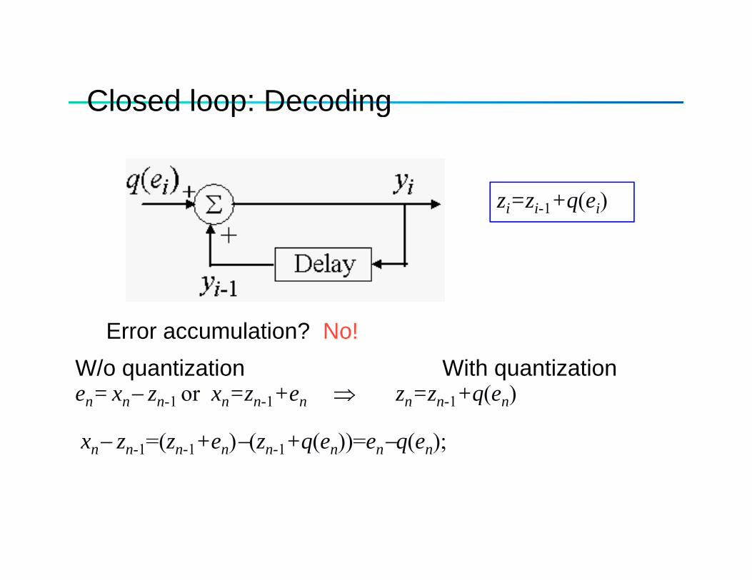
Closed loop: DecodingClosed loop: Decoding
zi=zi-1+q(ei)
Error acc m lation? No!Error accumulation? No!W/o quantization With quantizationen= xn− zn 1 or xn=zn 1+en ⇒ zn=zn 1+q(en)en xn zn-1 or xn zn-1 en ⇒ zn zn-1 q(en)
xn− zn-1=(zn-1+en)−(zn-1+q(en))=en−q(en);
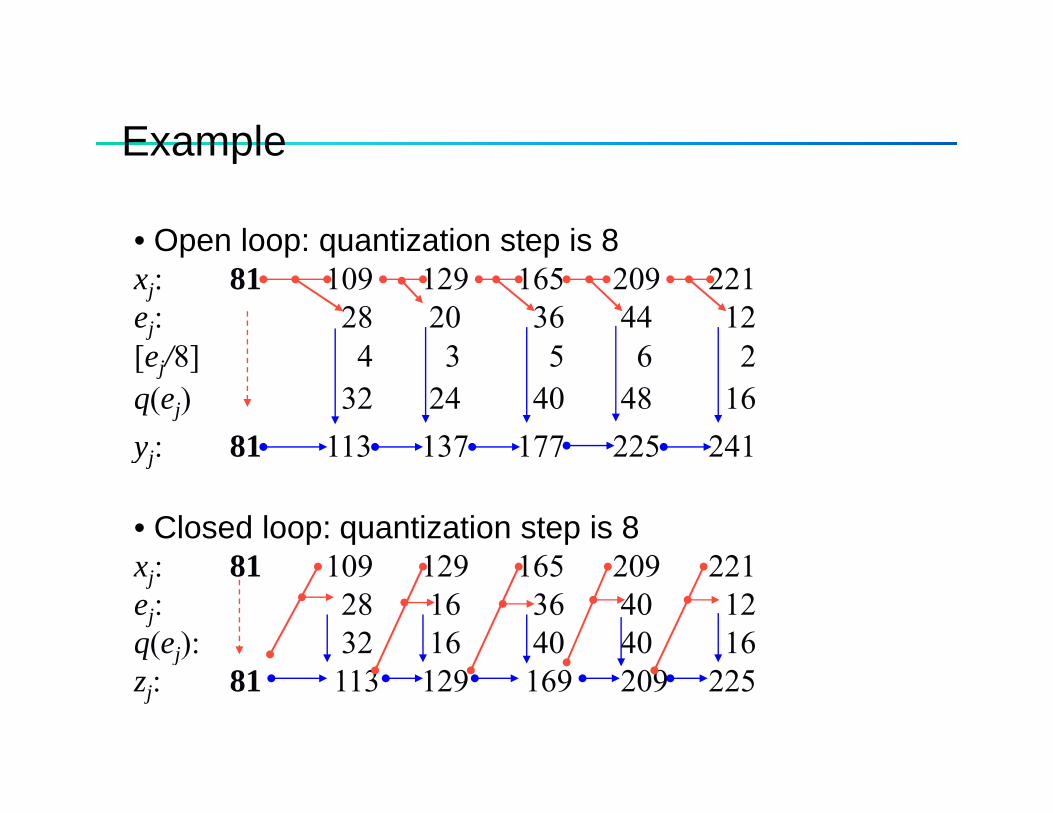
ExampleExample
• Open loop: quantization step is 8p p q pxj: 81 109 129 165 209 221ej: 28 20 36 44 12[e /8] 4 3 5 6 2[ej/8] 4 3 5 6 2q(ej) 32 24 40 48 16yj: 81 113 137 177 225 241yj
• Closed loop: quantization step is 881 109 129 165 209 221xj: 81 109 129 165 209 221
ej: 28 16 36 40 12q(ej): 32 16 40 40 16jzj: 81 113 129 169 209 225
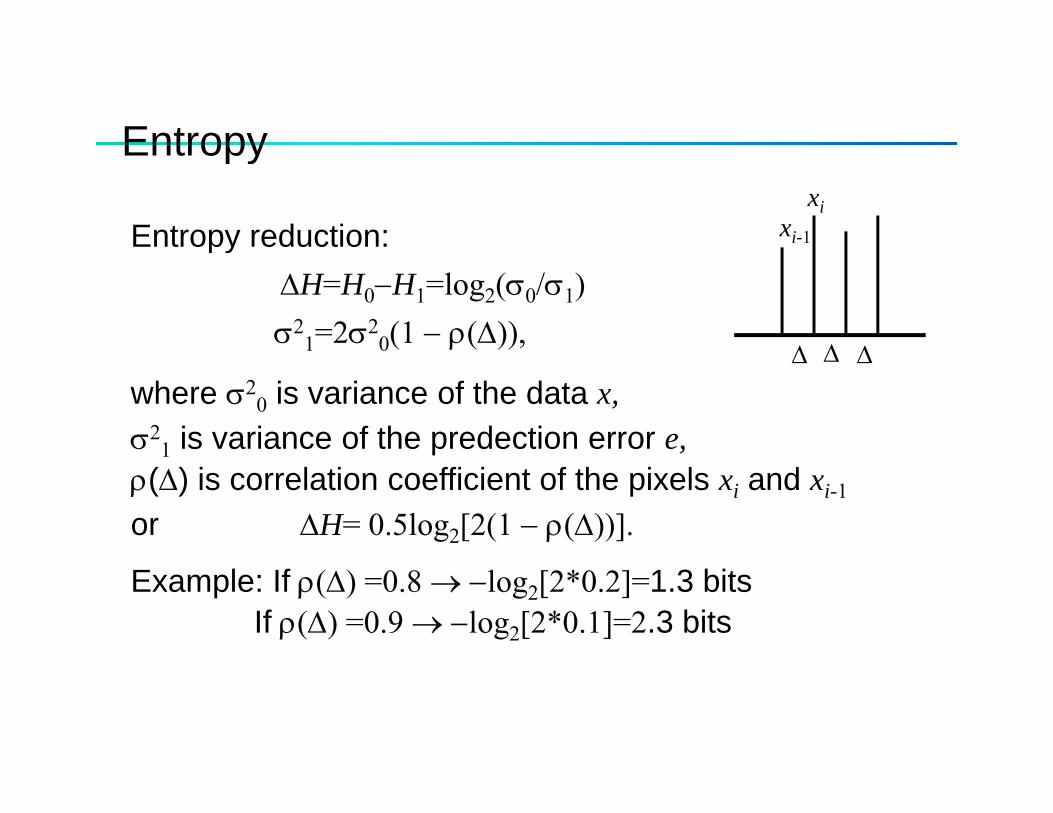
EntropyEntropy
Entropy reduction: xi-1
xi
pyΔH=H0−H1=log2(σ0/σ1)σ2
1=2σ20(1 − ρ(Δ)),
Δ Δ Δ
where σ20 is variance of the data x,
σ21 is variance of the predection error e,
Δ Δ Δ
ρ(Δ) is correlation coefficient of the pixels xi and xi-1
or ΔH= 0.5log2[2(1 − ρ(Δ))].
Example: If ρ(Δ) =0.8 → −log2[2*0.2]=1.3 bitsIf ρ(Δ) =0.9 → −log2[2*0.1]=2.3 bits
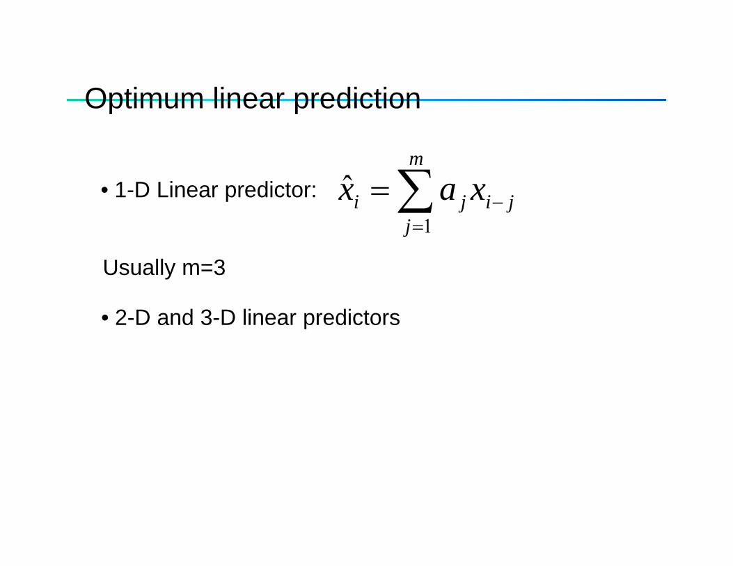
Optimum linear predictionOptimum linear prediction
∑m
ˆ ∑=
−=j
jiji xax1
ˆ• 1-D Linear predictor:
• 2-D and 3-D linear predictors
Usually m=3
• 2-D and 3-D linear predictors
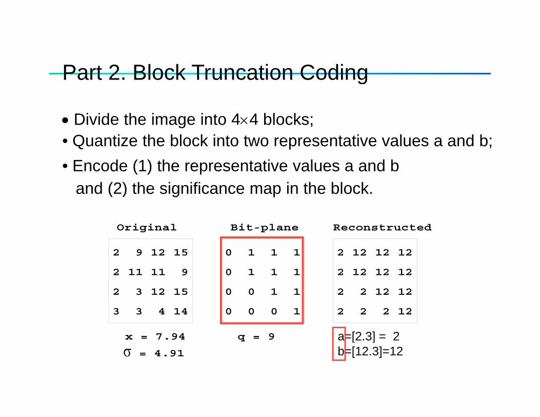
Part 2 Block Truncation CodingPart 2. Block Truncation Coding
• Divide the image into 4×4 blocks;• Quantize the block into two representative values a and b;• Encode (1) the representative values a and b
d (2) h i ifi i h bl kand (2) the significance map in the block.
Original Bit-plane Reconstructed
2 11 11 9
2 9 12 15
0 1 1 1
0 1 1 1
2 12 12 12
2 12 12 12
3 3 4 14
2 3 12 15
0 0 0 1
0 0 1 1
2 2 2 12
2 2 12 12
x = 7.94 q = 9 a = 2.3a=[2.3] = 2 = 4.91
q
b = 12.3σa [2.3] 2b=[12.3]=12
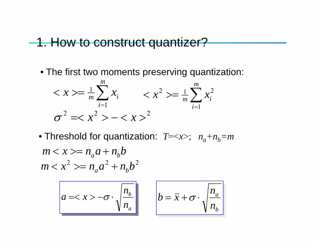
1 How to construct quantizer?1. How to construct quantizer?
• The first two moments preserving quantization: p g q
∑=
>=<m
iim xx
1
1 ∑>=<m
iim xx
1
212
i 1 =i 1222 ><−>=< xxσ
• Threshold for quantization: T=<x>; n +n =m• Threshold for quantization: T=<x>; na+nb=mbnanxm ba +>=<
222 bnanxm +>=<
bnxa ⋅−>=< σ anxb ⋅+= σ
bnanxm ba +>=<
anxa >=< σ
bnxb ⋅+= σ
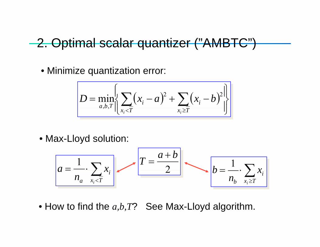
2 Optimal scalar quantizer (”AMBTC”)2. Optimal scalar quantizer ( AMBTC )
• Minimize quantization error:
( ) ( )⎪⎭
⎪⎬⎫
⎪⎩
⎪⎨⎧
−+−= ∑∑ iiTbabxaxD 22
,,min
⎪⎭⎪⎩ ≥< TxTxba
ii,,
• Max-Lloyd solution:
∑⋅= xa 1∑⋅= xb 12
baT +=
• Max-Lloyd solution:
∑<
=Tx
ia i
xn
a ∑≥
⋅=Tx
ib i
xn
b2
• How to find the a,b,T? See Max-Lloyd algorithm.
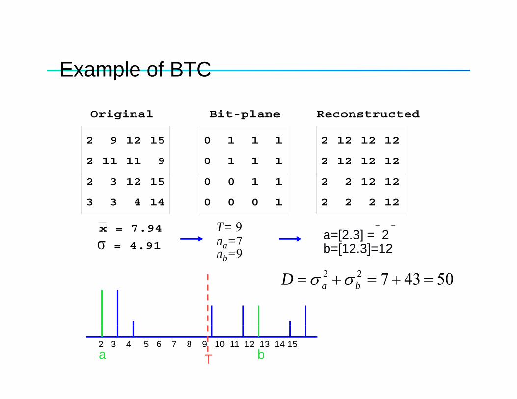
Example of BTCExample of BTC
Original Bit-plane Reconstructed
2 11 11 9
2 9 12 15
0 1 1 1
0 1 1 1
2 12 12 12
2 12 12 12
3 3 4 14
2 3 12 15
0 0 0 1
0 0 1 1
2 2 2 12
2 2 12 12
T 9x = 7.94
= 4.91
q = 9 a = 2.3
b = 12.3σT= 9na=7nb=9
5043722D
a=[2.3] = 2b=[12.3]=12
5043722 =+=+= baD σσ
2 3 4 5 6 7 8 9 10 11 12 13 14 15a bT
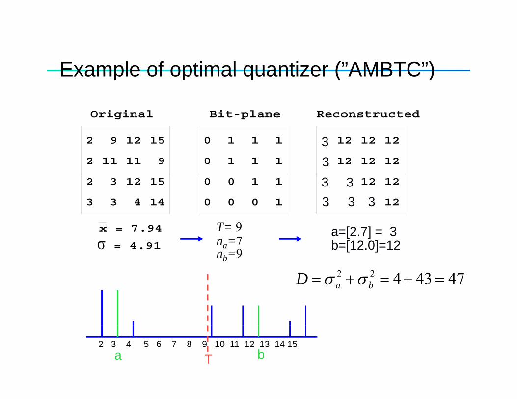
Example of optimal quantizer (”AMBTC”)Example of optimal quantizer ( AMBTC )
Original Bit-plane Reconstructed
2 11 11 9
2 9 12 15
0 1 1 1
0 1 1 1
2 12 12 12
2 12 12 1233
3 3 4 14
2 3 12 15
0 0 0 1
0 0 1 1
2 2 2 12
2 2 12 12
T 9
3 33 3 3
x = 7.94
= 4.91
q = 9 a = 2.3
b = 12.3σT= 9na=7nb=9
a=[2.7] = 3b=[12.0]=12
4743422D 4743422 =+=+= baD σσ
2 3 4 5 6 7 8 9 10 11 12 13 14 15ba T
Representative levels compressionRepresentative levels compression
Main idea of BTC:• Main idea of BTC:
Image → ”smooth part” + ”detailed part” (a and b) (bit-planes)(a and b) (bit-planes)
W t t t f ’ d b’ i• We can treat set of a’s and b’s as an image:1. Predictive encoding of a and b2 Lossless image compression algorithm2. Lossless image compression algorithm
(FELICS, JPEG-LS, CALIC). 3 Lossy compression: DCT (JPEG)3. Lossy compression: DCT (JPEG)
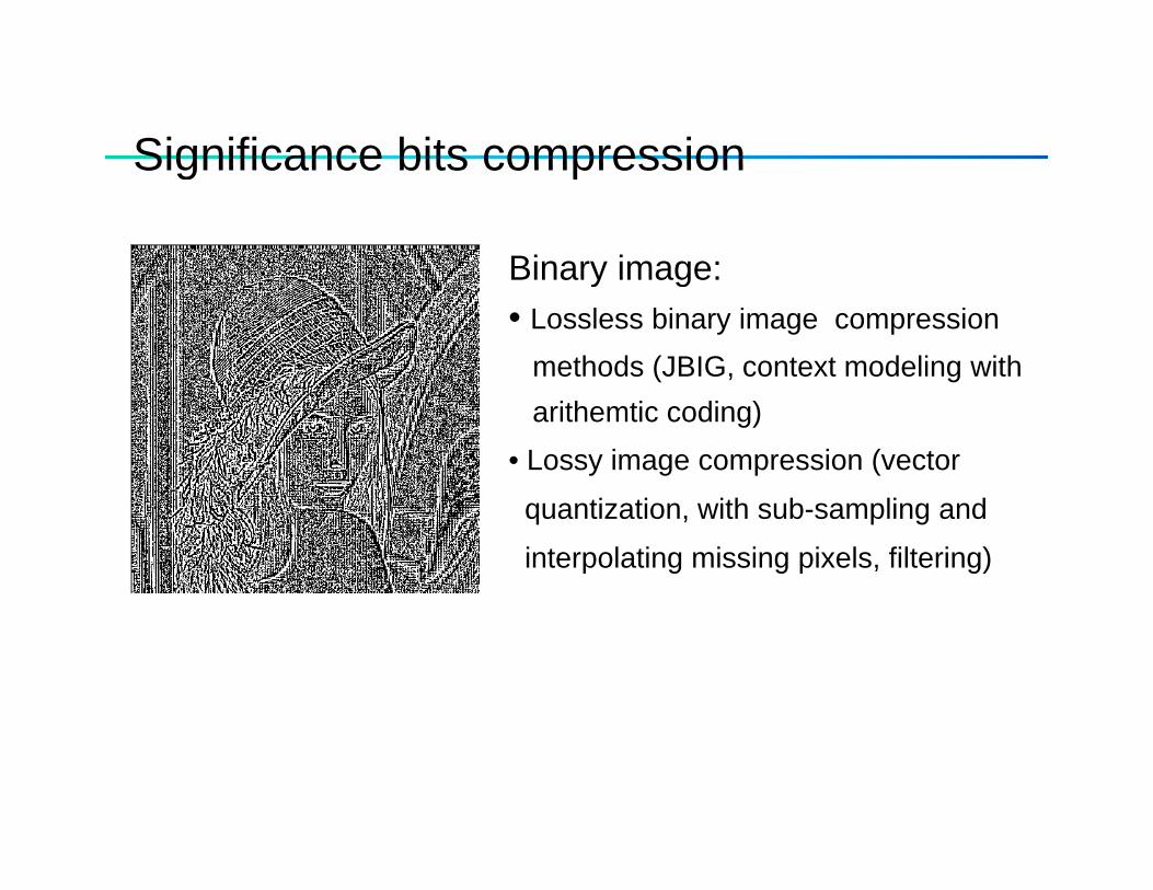
Significance bits compressionSignificance bits compression
Binary image:Binary image:• Lossless binary image compression
methods (JBIG, context modeling witharithemtic coding)
• Lossy image compression (vector
ti ti ith b li dquantization, with sub-sampling and
interpolating missing pixels, filtering)
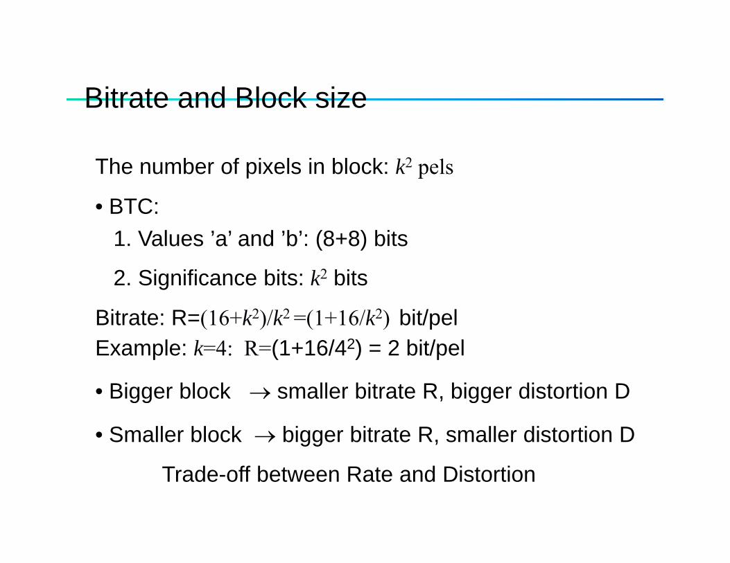
Bitrate and Block sizeBitrate and Block size
The number of pixels in block: k2 pelsp p
• BTC: 1. Values ’a’ and ’b’: (8+8) bitsa ues a a d b (8 8) b s
2. Significance bits: k2 bits
Bitrate: R=(16+k2)/k2 =(1+16/k2) bit/pelBitrate: R=(16+k2)/k2 =(1+16/k2) bit/pelExample: k=4: R=(1+16/42) = 2 bit/pel
• Bigger block → smaller bitrate R bigger distortion D• Bigger block → smaller bitrate R, bigger distortion D
• Smaller block → bigger bitrate R, smaller distortion D
Trade-off between Rate and Distortion
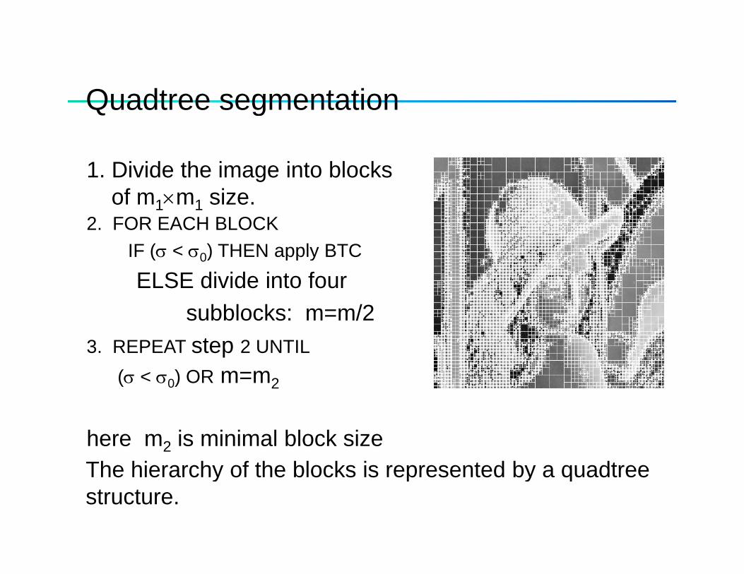
Quadtree segmentationQuadtree segmentation
1. Divide the image into blocks gof m1×m1 size.
2. FOR EACH BLOCKIF (σ < σ ) THEN apply BTCIF (σ < σ0) THEN apply BTC ELSE divide into four
subblocks: m=m/23. REPEAT step 2 UNTIL
(σ < σ0) OR m=m2
here m2 is minimal block sizeThe hierarchy of the blocks is represented by a quadtreeThe hierarchy of the blocks is represented by a quadtree structure.
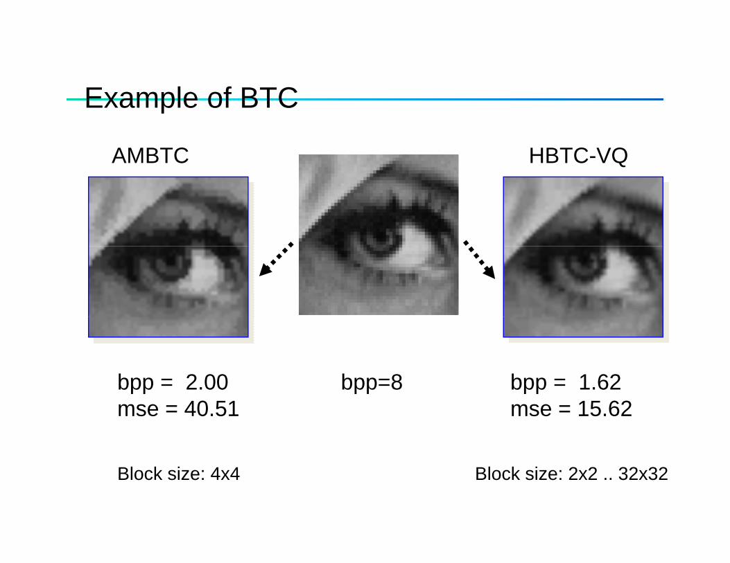
Example of BTCExample of BTC
AMBTC HBTC-VQ
bpp = 2.00 bpp=8 bpp = 1.62bpp 2.00 bpp 8 bpp 1.62mse = 40.51 mse = 15.62
Block size: 2x2 .. 32x32Block size: 4x4
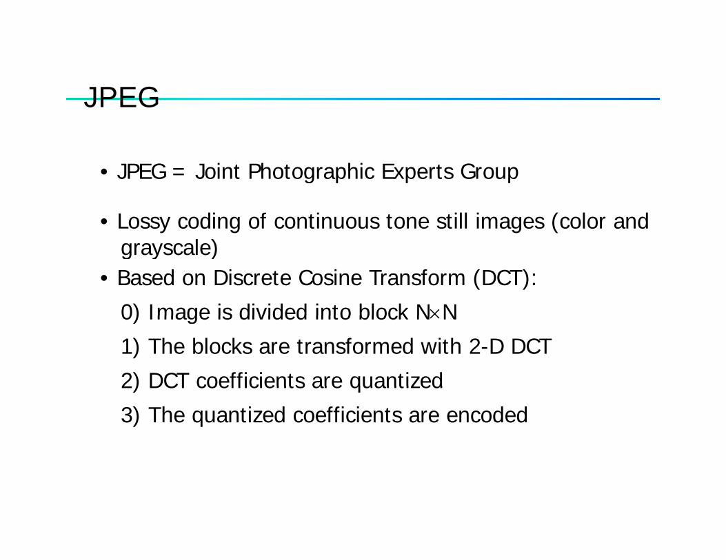
JPEGJPEG
• JPEG = Joint Photographic Experts Group• JPEG = Joint Photographic Experts Group
• Lossy coding of continuous tone still images (color andgrayscale)grayscale)
• Based on Discrete Cosine Transform (DCT):
0) Image is divided into block N×N0) Image is divided into block N×N
1) The blocks are transformed with 2-D DCT
2) DCT coefficients are quantized2) DCT coefficients are quantized
3) The quantized coefficients are encoded
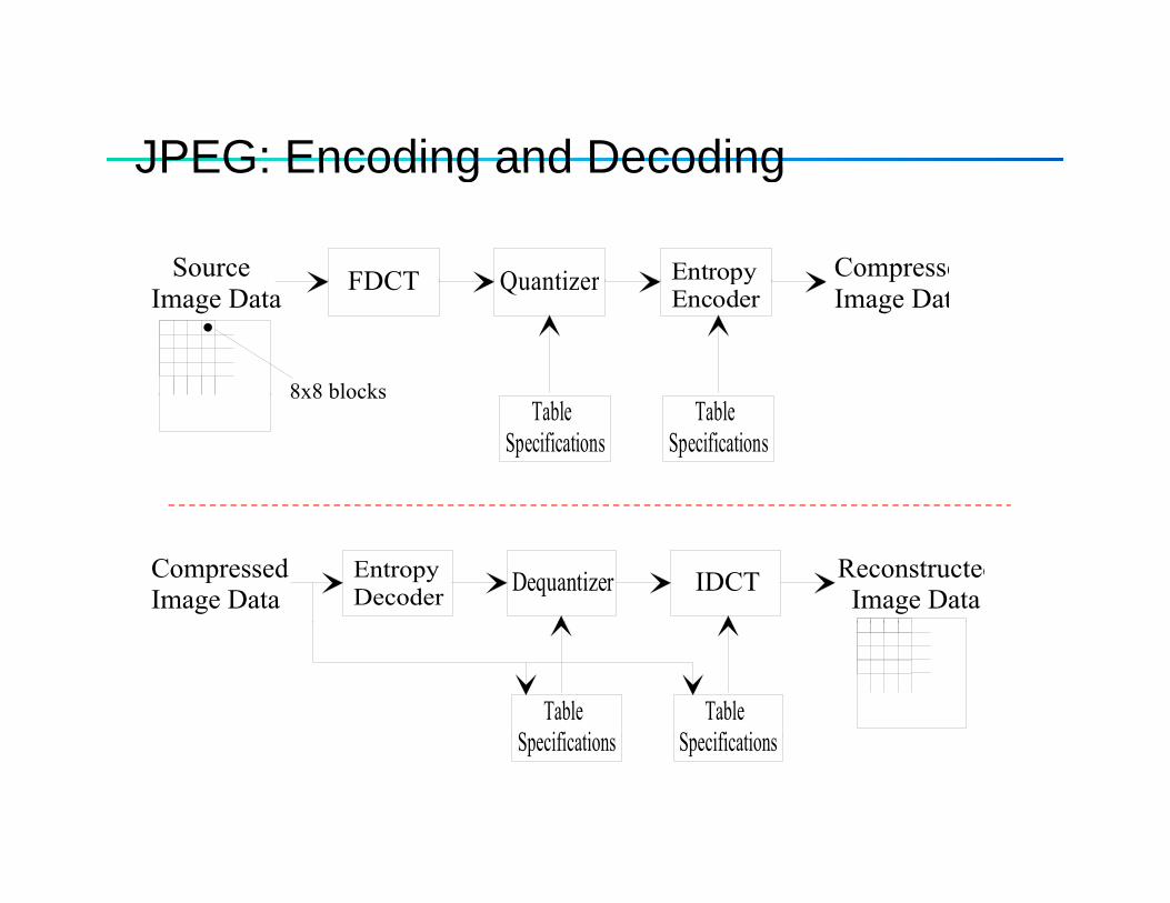
JPEG: Encoding and DecodingJPEG: Encoding and Decoding
Source FDCT Quantizer Entropy CompresseImage Data
8x8 blocks
FDCT Quantizer pyEncoder
pImage Dat
8x8 blocks TableSpecifications
TableSpecifications
IDCTDequantizerEntropyDecoder
Reconstructed Image Data
CompressedImage Data
TableS ifi ti
TableS ifi tiSpecifications Specifications
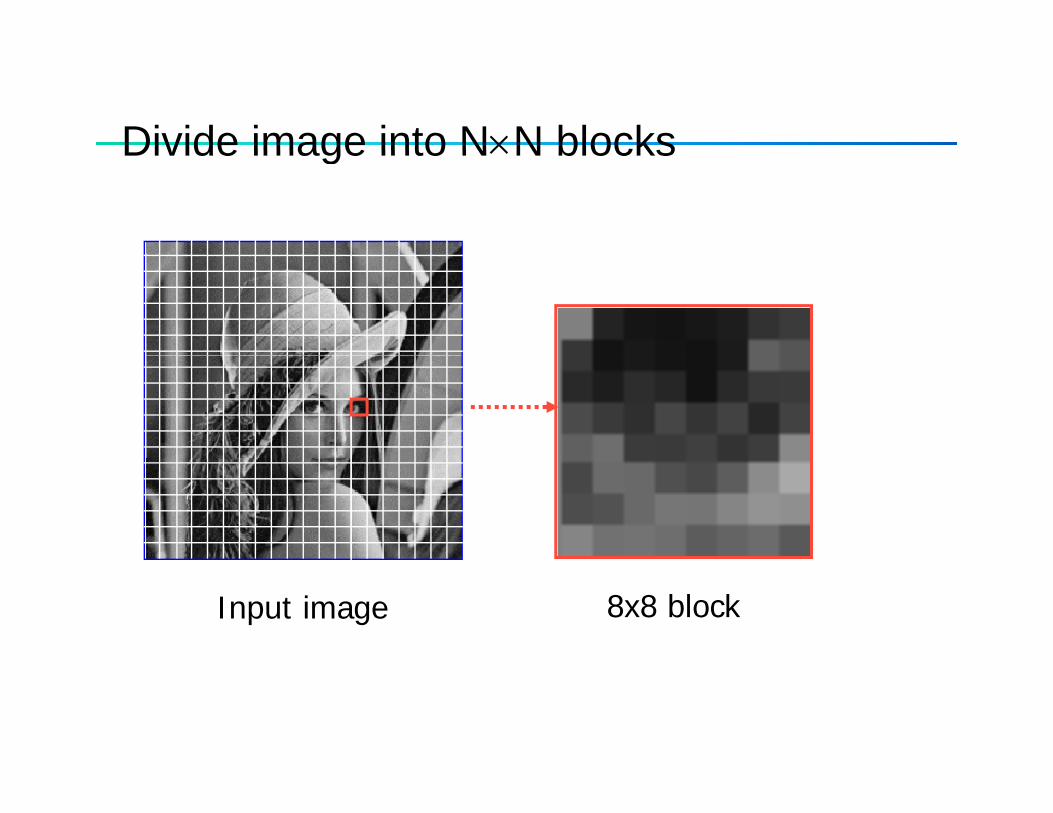
Divide image into N×N blocksDivide image into N×N blocks
8x8 blockInput image
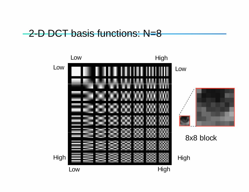
2-D DCT basis functions: N=82 D DCT basis functions: N 8
Low Higho
LowHigh
Low
High High
8x8 block
High High
HighLow
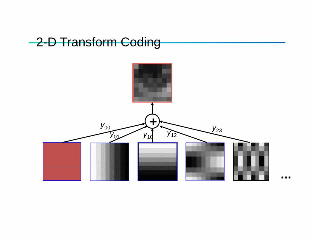
2-D Transform Coding2 D Transform Coding
+y00y01 y10
y12y23y01 y10
y12
...
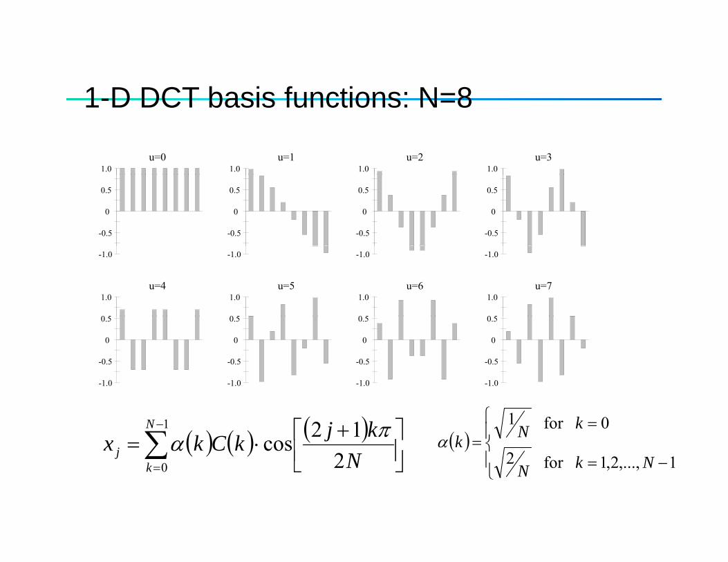
1-D DCT basis functions: N=81 D DCT basis functions: N 8
1.0u=0
1.0u=1
1.0u=2
1.0u=3
0.5
0
-0.5
0.5
0
-0.5
0.5
0
-0.5
0.5
0
-0.5
-1.0 -1.0 -1.0 -1.0
1.0
0 5
u=41.0
0 5
u=51.0
0 5
u=61.0
0 5
u=7
0.5
0
-0.5
-1.0
0.5
0
-0.5
-1.0
0.5
0
-0.5
-1.0
0.5
0
-0.5
-1.0
( ) ( ) ( )∑−
⎥⎦⎤
⎢⎣⎡ +
⋅=1
212cos
N
j NkjkCkx πα ( )
⎪
⎪⎨
⎧ ==
121f2
0for 1
Nk
kNkα∑=
⎥⎦⎢⎣0 2kj N ⎪
⎩−= 1,...,2,1for 2 NkN
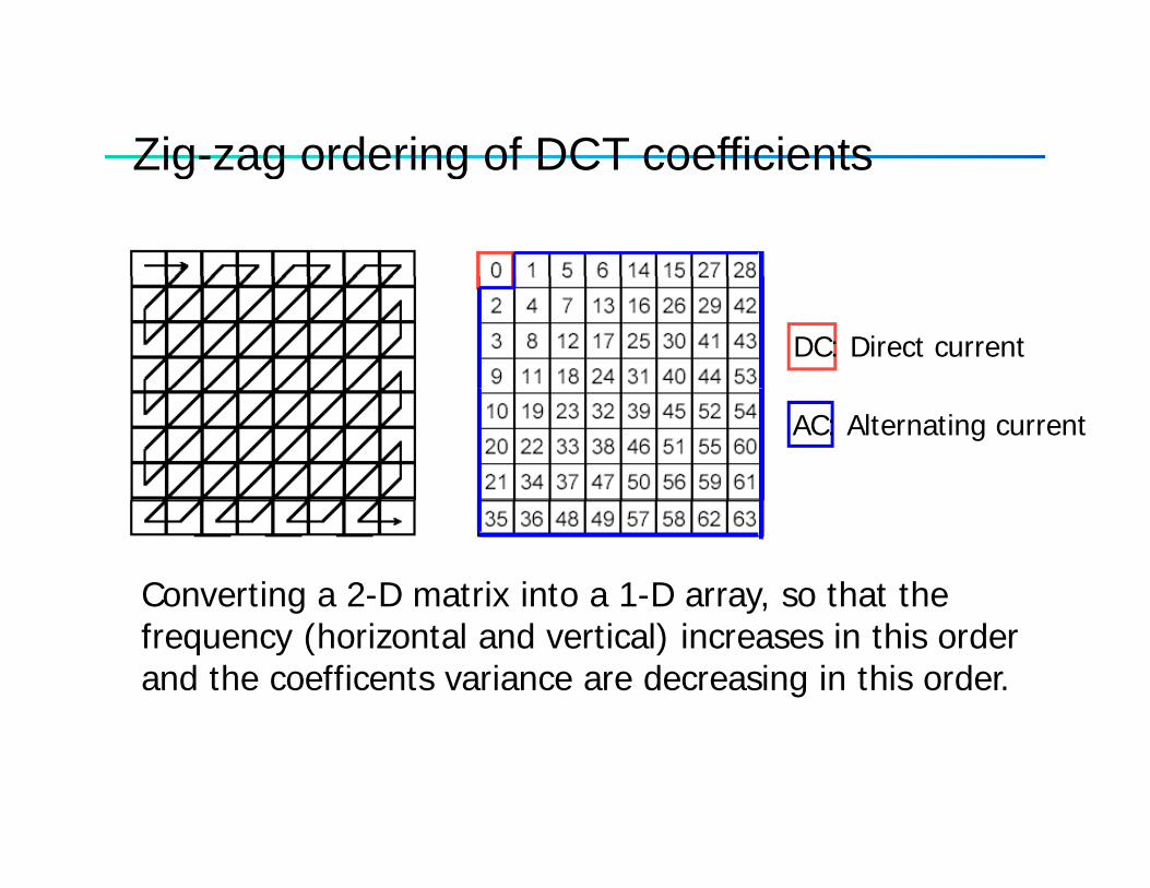
Zig-zag ordering of DCT coefficientsZig zag ordering of DCT coefficients
DC: Direct current
AC: Alternating current
Converting a 2-D matrix into a 1-D array, so that the g y,frequency (horizontal and vertical) increases in this orderand the coefficents variance are decreasing in this order.
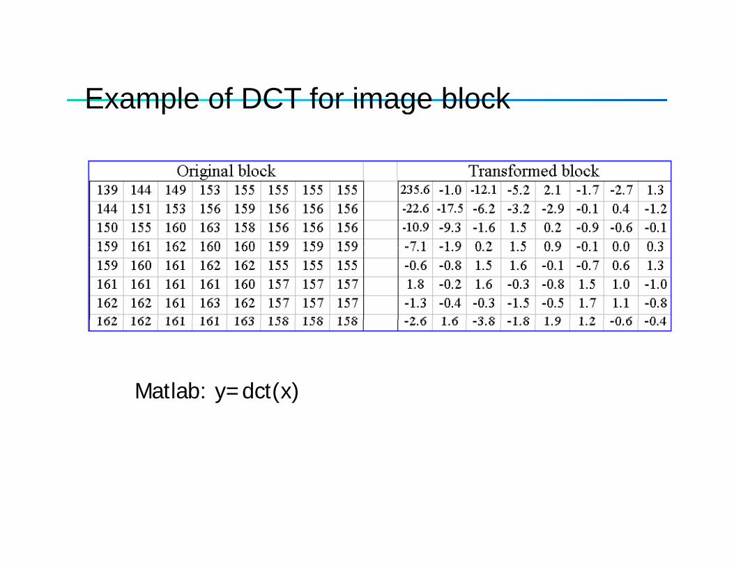
Example of DCT for image blockExample of DCT for image block
Matlab: y=dct(x)Matlab: y=dct(x)
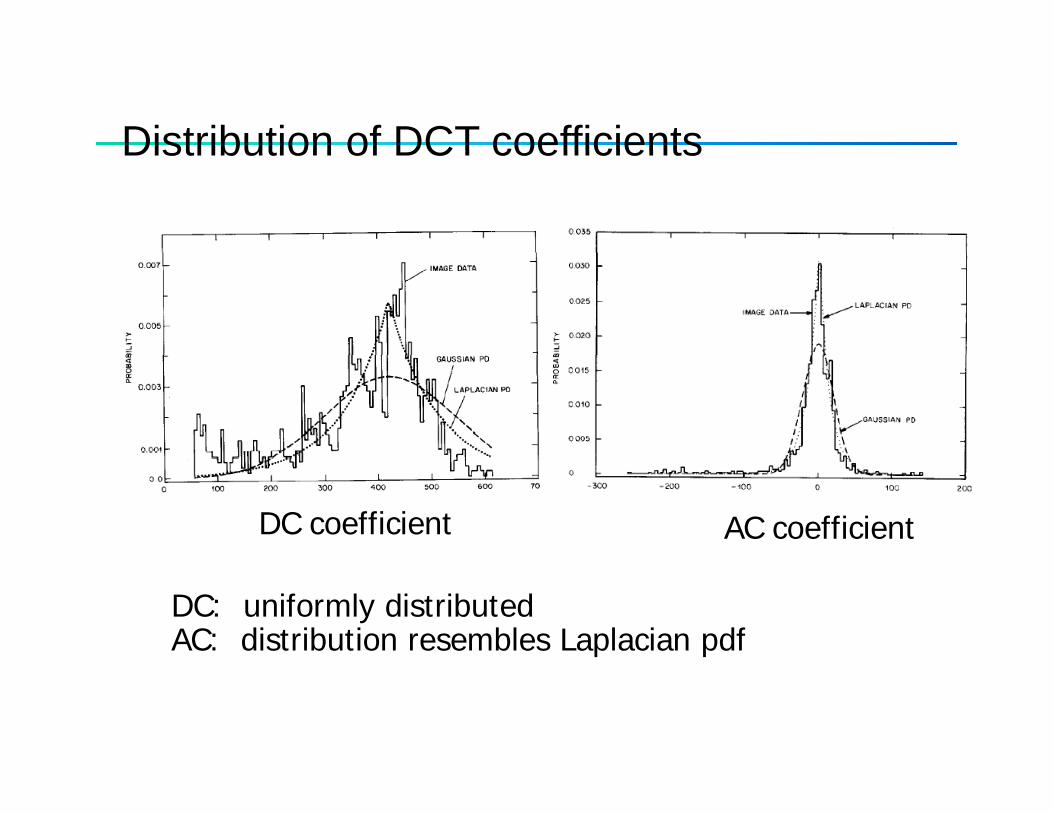
Distribution of DCT coefficientsDistribution of DCT coefficients
DC coefficient AC coefficient
DC: uniformly distributedAC: distribution resembles Laplacian pdf
Bit allocation for DCT coefficientsBit allocation for DCT coefficients
• Lossy operation to reduce bit-rate• Lossy operation to reduce bit rate• Vector or Scalar Quantizer?
• Set of optimal scalar quantizers?p q• Set of scalar quantizers with fixed quantization tables
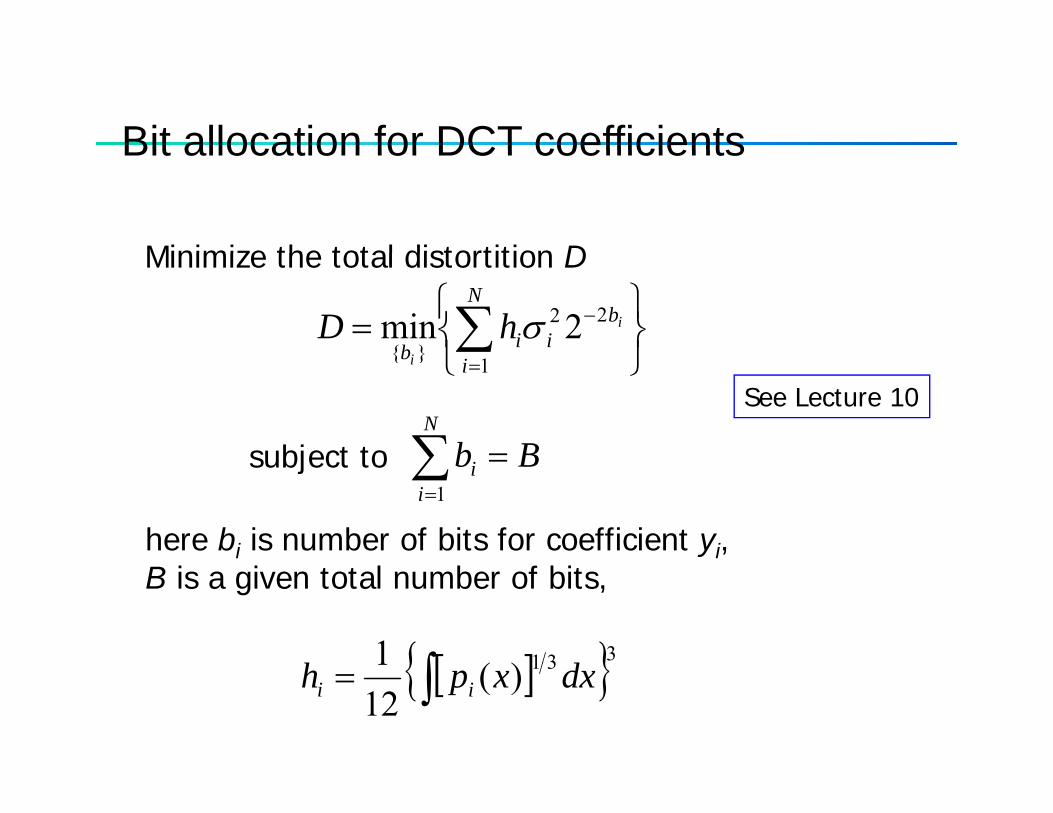
Bit allocation for DCT coefficientsBit allocation for DCT coefficients
Minimize the total distortition D
⎭⎬⎫
⎩⎨⎧
= ∑ −N
biib
i
i
hD 22
}{2min σ
Minimize the total distortition D
⎭⎩ =ibi 1}{
subject to BbN
=∑See Lecture 10
subject to Bbi
i =∑=1
here bi is number of bits for coefficient yi,
[ ]{ }331)(1∫ dh
B is a given total number of bits,
[ ]{ }31)(121
∫= dxxph ii
Optimal bit allocation for DCT coefficientsOptimal bit allocation for DCT coefficients
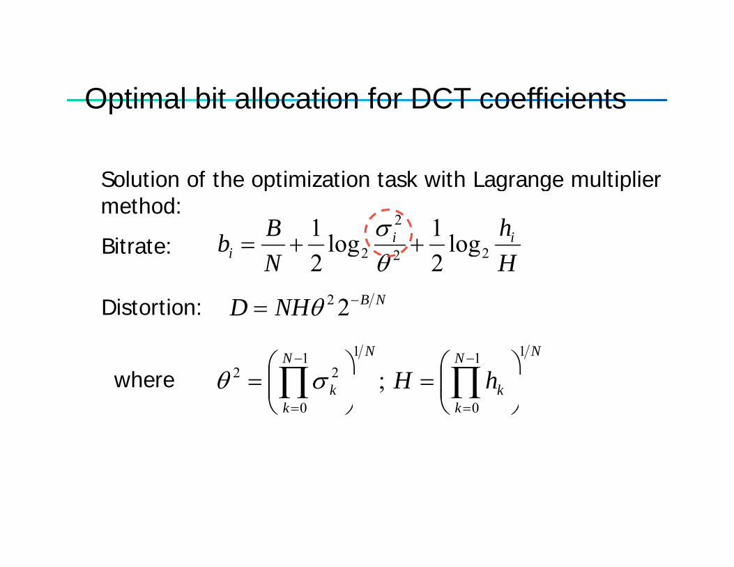
Solution of the optimization task with Lagrange multiplier
hBb ii2
log1log1++=
σ
Solution of the optimization task with Lagrange multiplier method:
Bitrate:HN
bi 222 log2
log2
++=θNBNHD −= 22θ
Bitrate:
Distortion:
NN
k
NN
k hH1111
22 ; ⎟⎟⎠
⎞⎜⎜⎝
⎛=⎟⎟
⎠
⎞⎜⎜⎝
⎛= ∏∏
−−
σθwherek
kk
k00
; ⎟⎠
⎜⎝
⎟⎠
⎜⎝
∏∏==
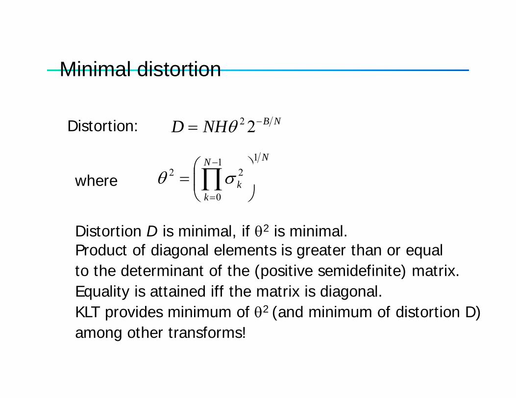
Minimal distortionMinimal distortion
NBNHD −22θDistortion:
NN 1122⎟⎟⎞
⎜⎜⎛∏
−
θ
NBNHD = 22θDistortion:
hk
k0
22⎟⎟⎠
⎜⎜⎝
= ∏=
σθwhere
2Distortion D is minimal, if θ2 is minimal. Product of diagonal elements is greater than or equal to the determinant of the (positive semidefinite) matrix.to the determinant of the (positive semidefinite) matrix.Equality is attained iff the matrix is diagonal. KLT provides minimum of θ2 (and minimum of distortion D)among other transforms!
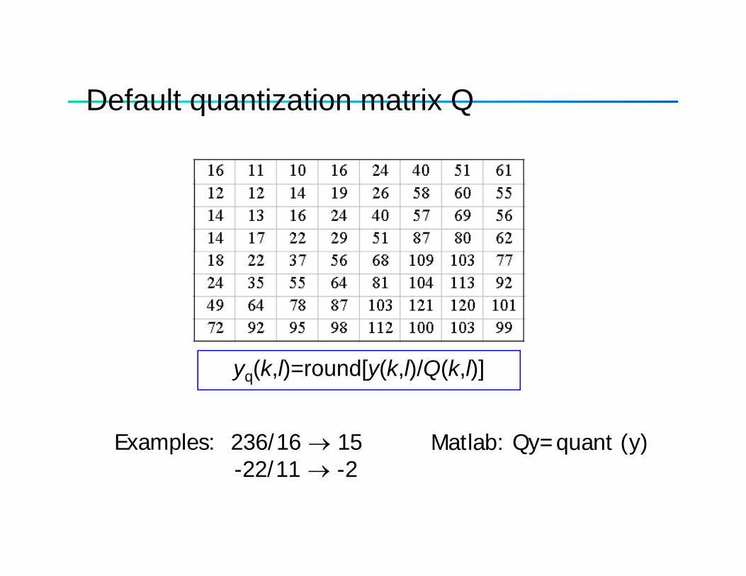
Default quantization matrix QDefault quantization matrix Q
yq(k,l)=round[y(k,l)/Q(k,l)]
Examples: 236/16 → 15-22/11 → -2
Matlab: Qy=quant (y)-22/11 → -2
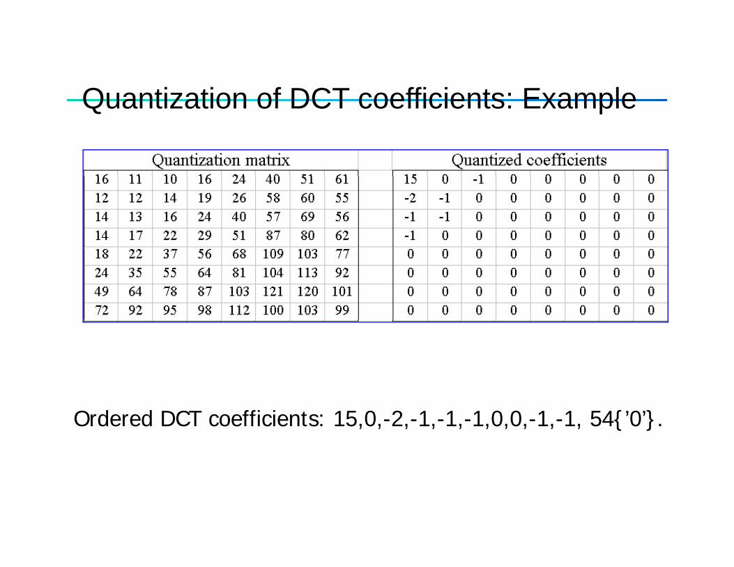
Quantization of DCT coefficients: ExampleQuantization of DCT coefficients: Example
Ordered DCT coefficients: 15,0,-2,-1,-1,-1,0,0,-1,-1, 54{’0’}.
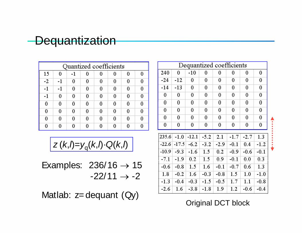
DequantizationDequantization
z (k,l)=yq(k,l)·Q(k,l)
Examples: 236/16 → 15-22/11 → -2
Original DCT blockMatlab: z=dequant (Qy)
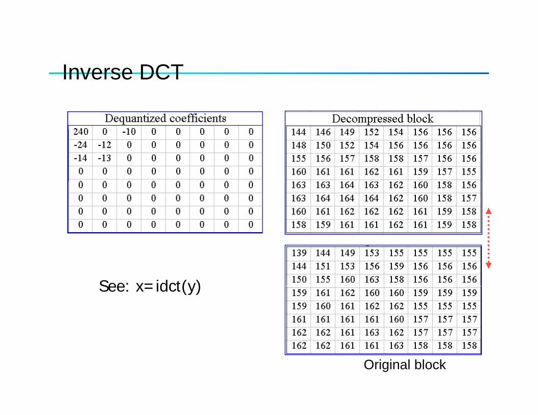
Inverse DCTInverse DCT
See: x=idct(y)See: x=idct(y)
Original block
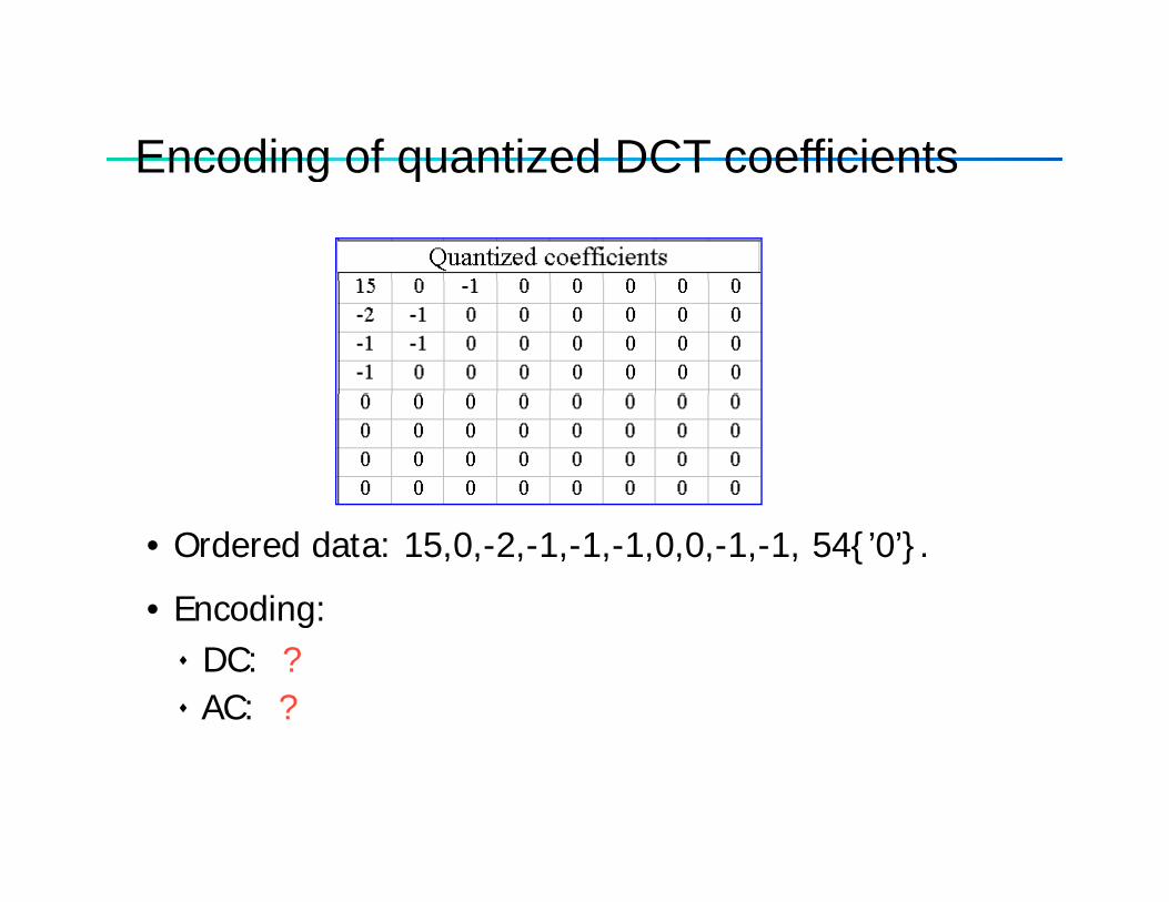
Encoding of quantized DCT coefficientsEncoding of quantized DCT coefficients
• Ordered data: 15,0,-2,-1,-1,-1,0,0,-1,-1, 54{’0’}.
• Encoding: g♦ DC: ?♦ AC: ?
Encoding of quantized DCT coefficientsEncoding of quantized DCT coefficients
• DC coefficient for the current block is predicted of that of the previous block, and error is coded usingHuffman coding
• AC coefficients:
(a) Huffman code, arithmetic code for non-zeroes( ) ,(b) run-length encoding: (number of ’0’s, non-’0’-symbol)
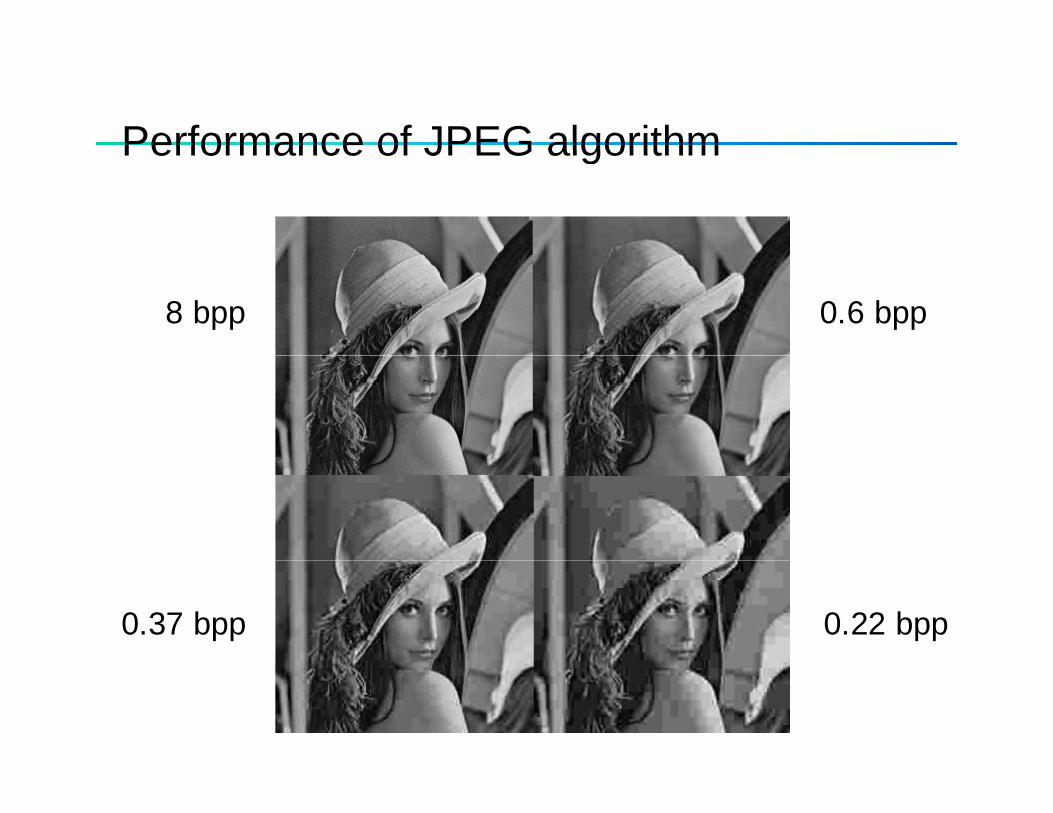
Performance of JPEG algorithmPerformance of JPEG algorithm
8 bpp 0.6 bpp
0.37 bpp 0.22 bpp
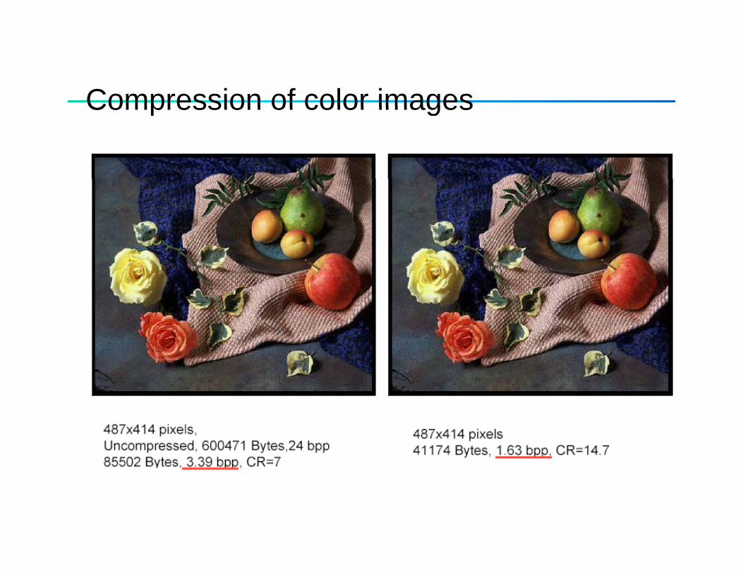
Compression of color imagesCompression of color images
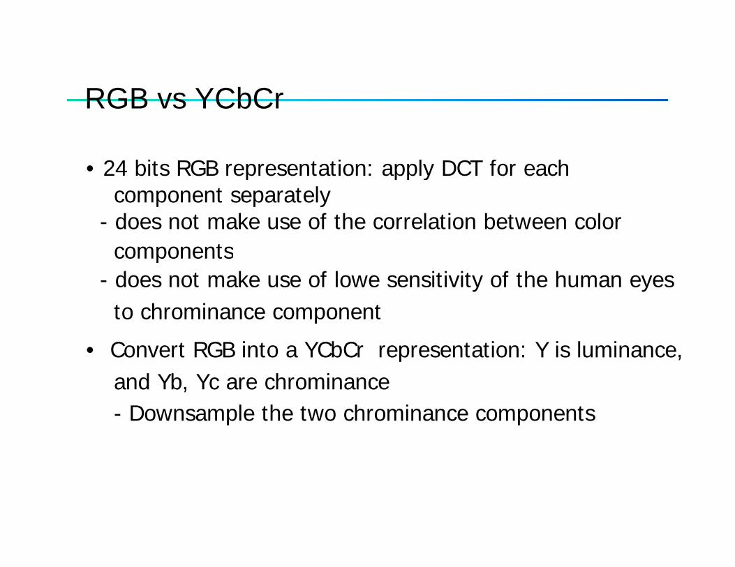
RGB vs YCbCrRGB vs YCbCr
• 24 bits RGB representation: apply DCT for each p pp ycomponent separately
- does not make use of the correlation between color componentscomponents
- does not make use of lowe sensitivity of the human eyes to chrominance componentto c o a ce co po e t
• Convert RGB into a YCbCr representation: Y is luminance,and Yb, Yc are chrominance,- Downsample the two chrominance components
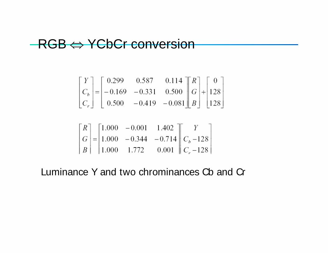
RGB ⇔ YCbCr conversionRGB ⇔ YCbCr conversion
Luminance Y and two chrominances Cb and CrLuminance Y and two chrominances Cb and Cr
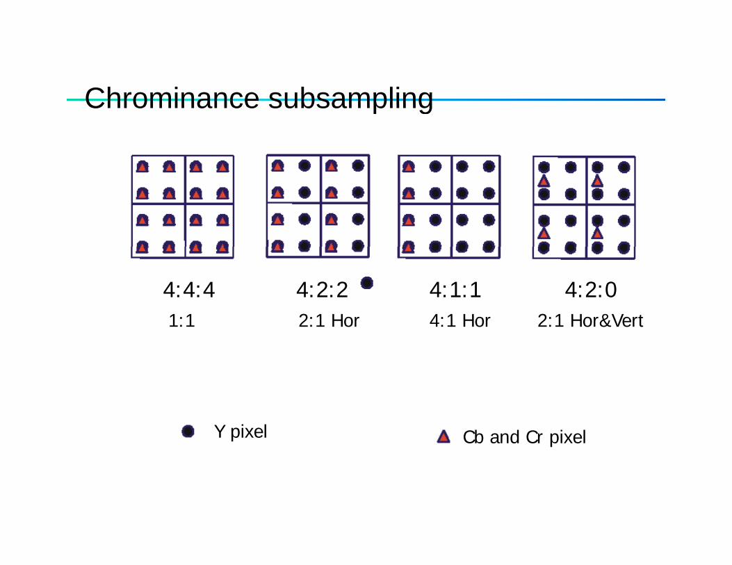
Chrominance subsamplingChrominance subsampling
4:4:4 4:2:2 4:1:1 4:2:01:1 2:1 Hor 4:1 Hor 2:1 Hor&Vert1:1 2:1 Hor 4:1 Hor 2:1 Hor&Vert
Cb and Cr pixelY pixel
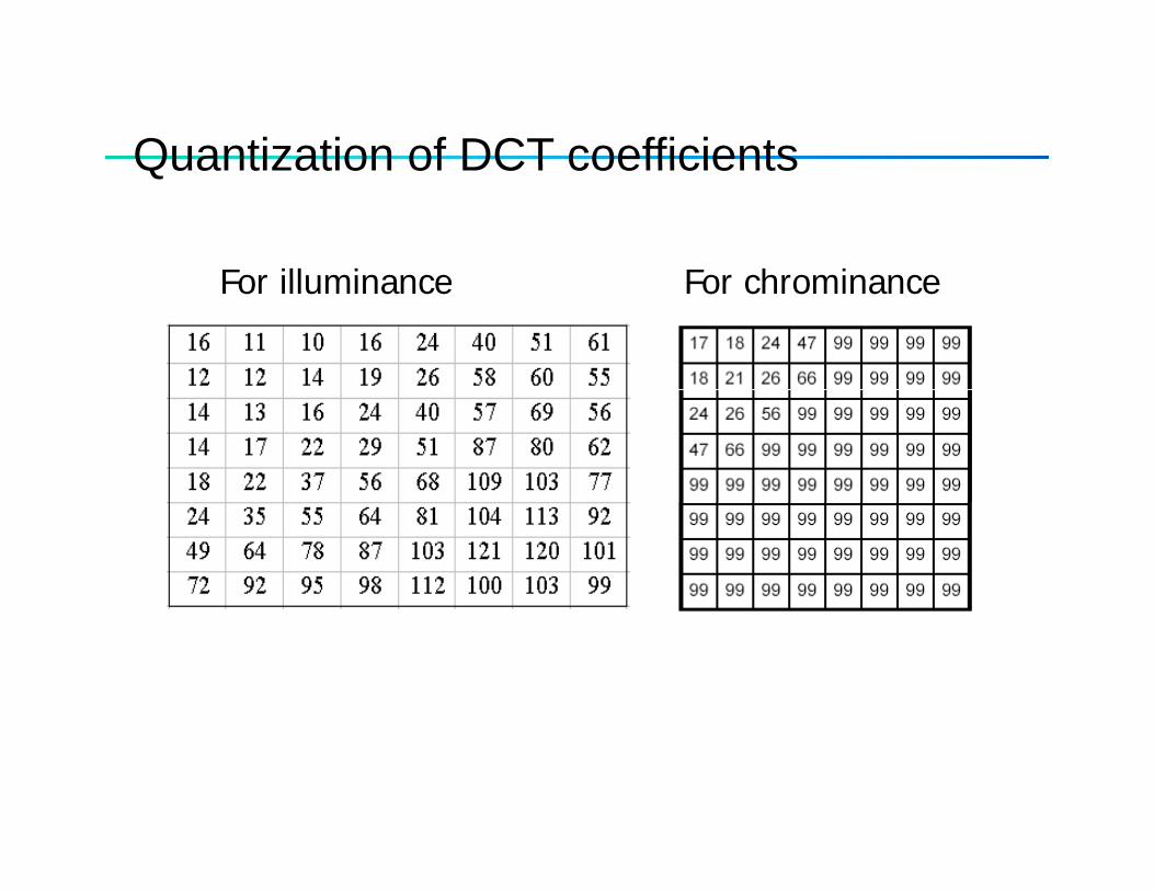
Quantization of DCT coefficientsQuantization of DCT coefficients
For chrominanceFor illuminance For chrominance For illuminance
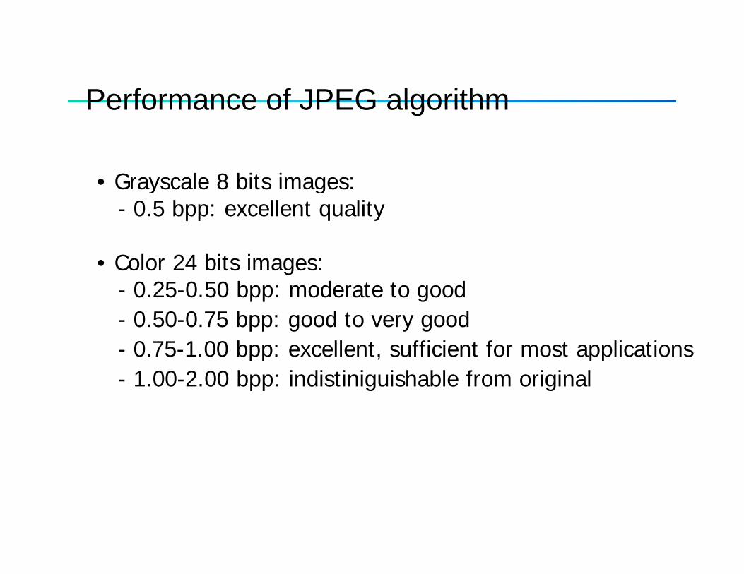
Performance of JPEG algorithmPerformance of JPEG algorithm
• Grayscale 8 bits images:• Grayscale 8 bits images: - 0.5 bpp: excellent quality
• Color 24 bits images: - 0.25-0.50 bpp: moderate to good - 0 50-0 75 bpp: good to very good0.50 0.75 bpp: good to very good- 0.75-1.00 bpp: excellent, sufficient for most applications - 1.00-2.00 bpp: indistiniguishable from original
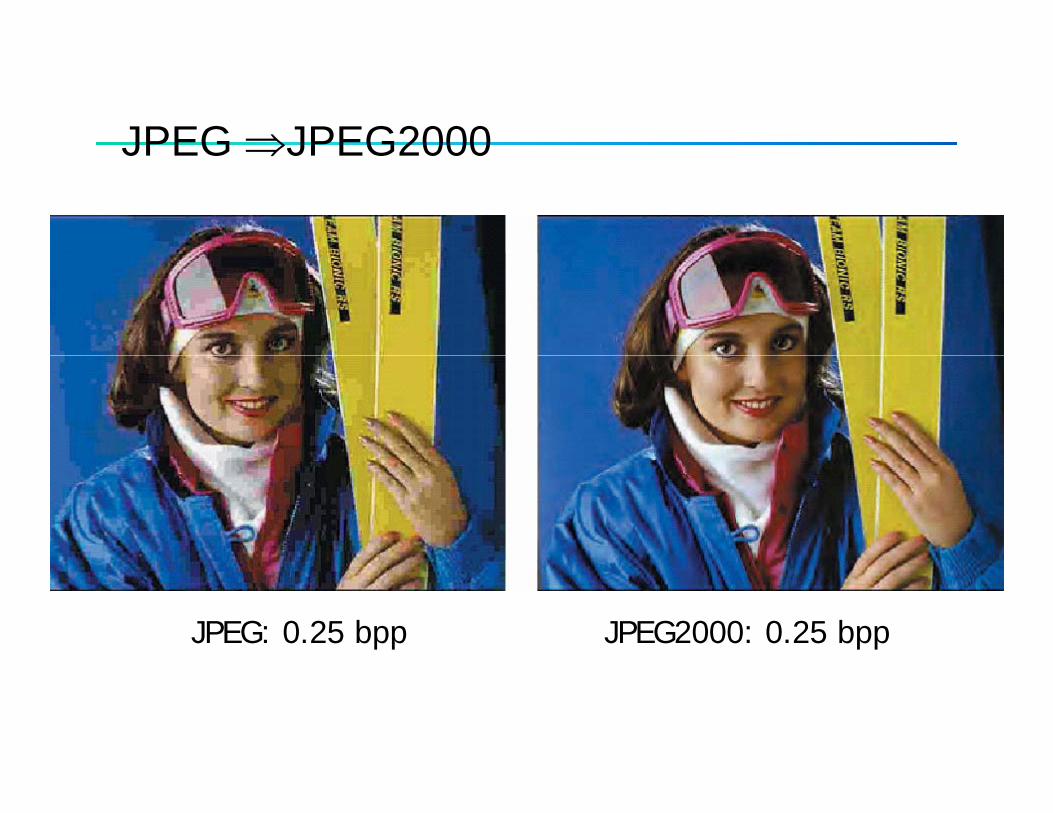
JPEG ⇒JPEG2000JPEG ⇒JPEG2000
For illuminanceFor illuminance
JPEG: 0.25 bpp JPEG2000: 0.25 bpp
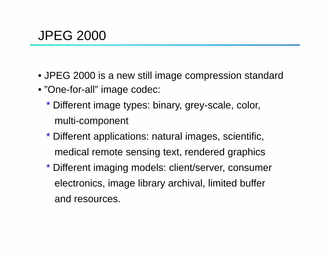
JPEG 2000
• JPEG 2000 is a new still image compression standardg p• ”One-for-all” image codec:
* Different image types: binary, grey-scale, color, multi-component
* Different applications: natural images, scientific, medical remote sensing text, rendered graphics
* Different imaging models: client/server, consumer electronics, image library archival, limited buffer and resources.
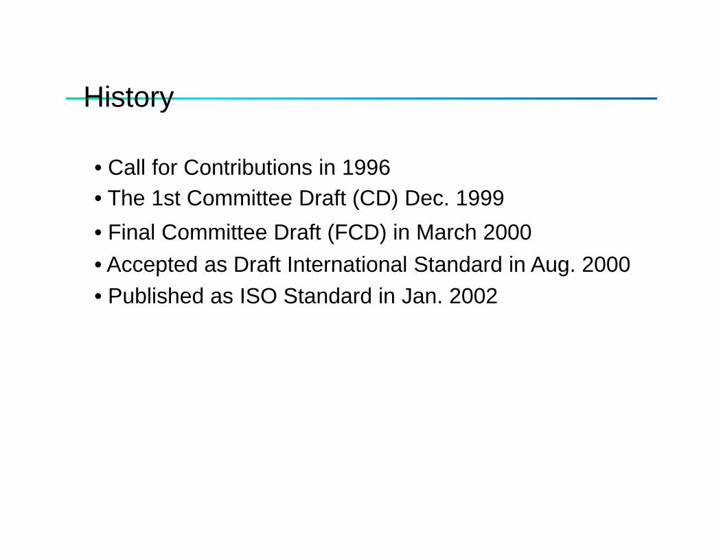
HistoryHistory
• Call for Contributions in 1996Call for Contributions in 1996• The 1st Committee Draft (CD) Dec. 1999• Final Committee Draft (FCD) in March 2000( )• Accepted as Draft International Standard in Aug. 2000• Published as ISO Standard in Jan. 2002
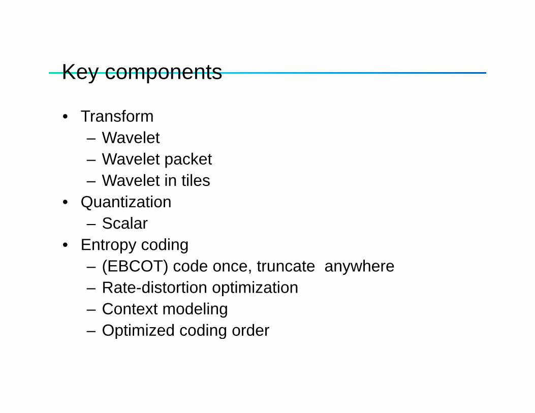
Key componentsKey components
• Transform– Wavelet – Wavelet packet
Wavelet in tiles– Wavelet in tiles• Quantization
– Scalar • Entropy coding
– (EBCOT) code once, truncate anywhere Rate distortion optimization– Rate-distortion optimization
– Context modeling– Optimized coding orderp g
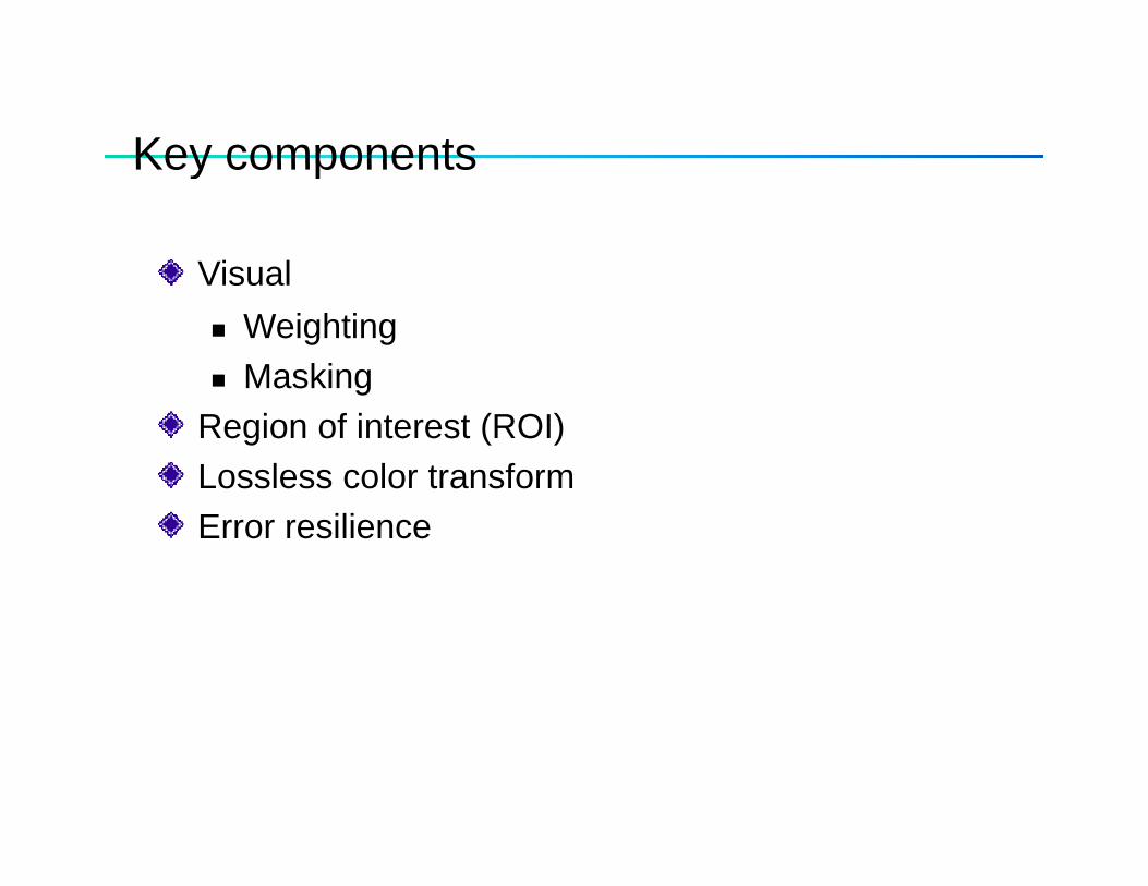
Key componentsKey components
VisualVisualWeightingMaskingMasking
Region of interest (ROI)Lossless color transformError resilience
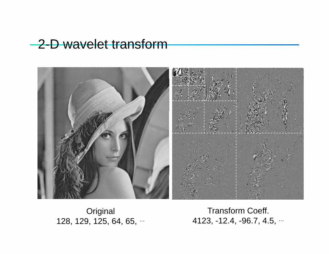
2-D wavelet transform2 D wavelet transform
Original128, 129, 125, 64, 65, …
Transform Coeff.4123, -12.4, -96.7, 4.5, …
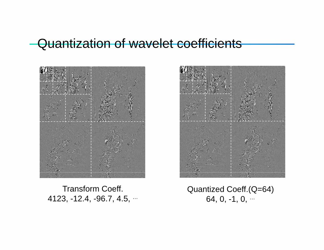
Quantization of wavelet coefficientsQuantization of wavelet coefficients
Transform Coeff.4123, -12.4, -96.7, 4.5, …
Quantized Coeff.(Q=64)64, 0, -1, 0, …
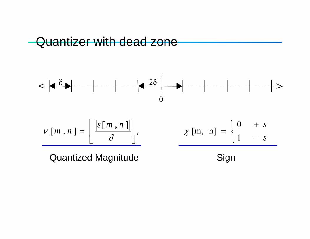
Quantizer with dead zoneQuantizer with dead zone
2δ
0
δ
⎩⎨⎧ +
=⎥⎥
⎢⎢
=snms
nm10
n][m, ,],[
],[ χδ
ν⎩⎨ −⎥
⎦⎢⎣ s1
][ ,,],[ χδ
Quantized Magnitude Sign
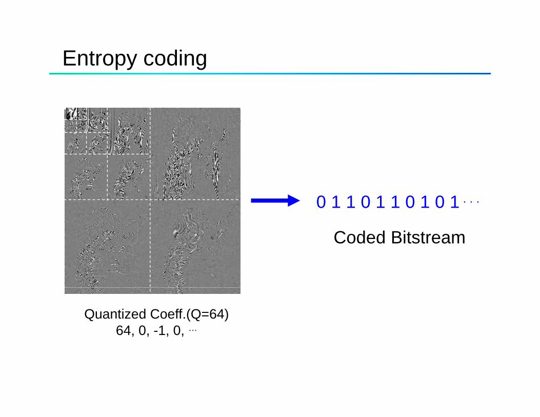
Entropy coding
0 1 1 0 1 1 0 1 0 1 . . .
Coded BitstreamCoded Bitstream
Quantized Coeff.(Q=64)64, 0, -1, 0, …
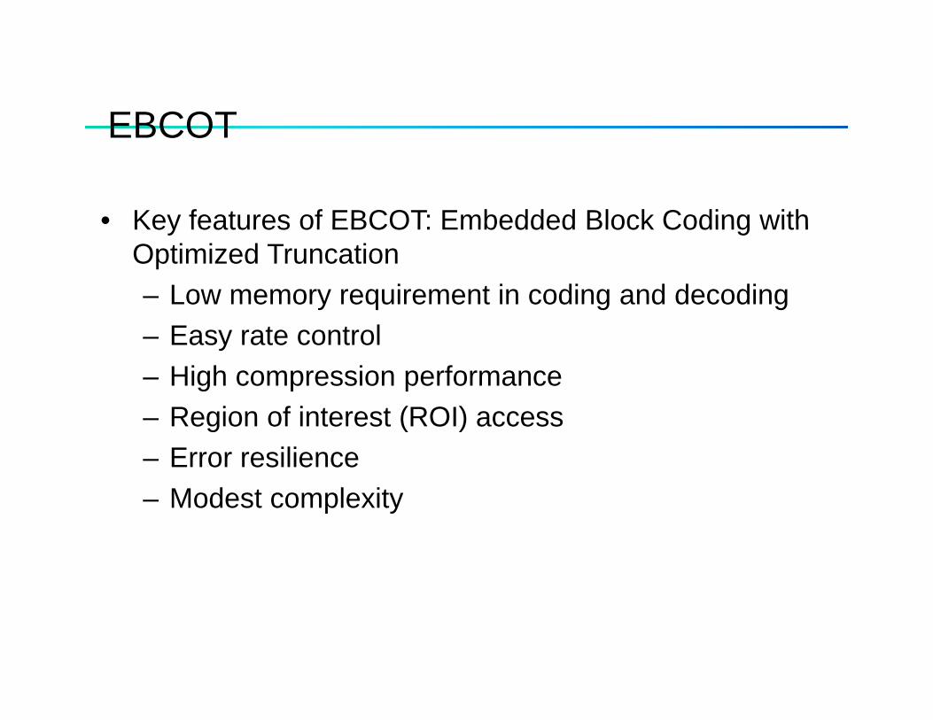
EBCOTEBCOT
• Key features of EBCOT: Embedded Block Coding withKey features of EBCOT: Embedded Block Coding with Optimized Truncation– Low memory requirement in coding and decoding– Easy rate control– High compression performance– Region of interest (ROI) access– Error resilience
Modest complexity– Modest complexity
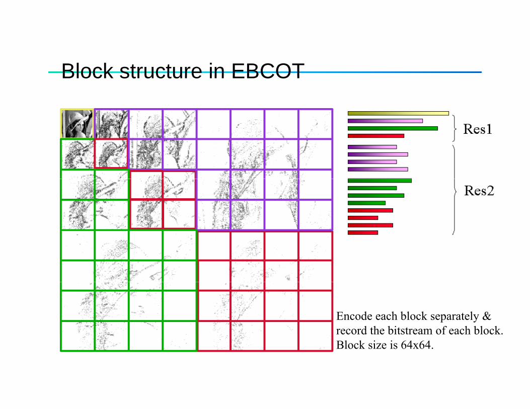
Block structure in EBCOTBlock structure in EBCOT
Encode each block separately & record the bitstream of each block.record the bitstream of each block.Block size is 64x64.
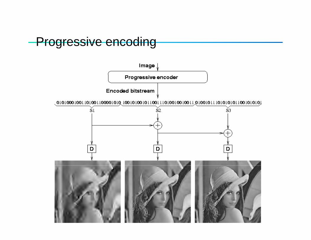
Progressive encodingProgressive encoding

Quantizer with dead zoneQuantizer with dead zone
2δ
0
δ
⎩⎨⎧ +
=⎥⎥
⎢⎢
=snms
nm10
n][m, ,],[
],[ χδ
ν⎩⎨ −⎥
⎦⎢⎣ s1
][ ,,],[ χδ
Quantized Magnitude Sign
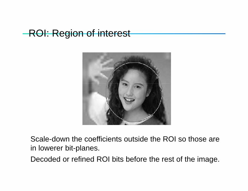
ROI: Region of interestROI: Region of interest
Scale-down the coefficients outside the ROI so those are in lowerer bit-planes.Decoded or refined ROI bits before the rest of the image.
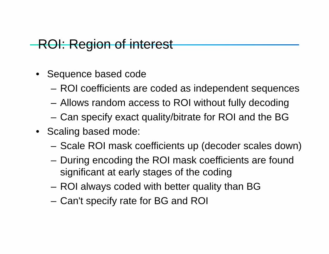
ROI: Region of interestROI: Region of interest
• Sequence based codeq– ROI coefficients are coded as independent sequences– Allows random access to ROI without fully decoding– Can specify exact quality/bitrate for ROI and the BG
• Scaling based mode:S l ROI k ffi i t (d d l d )– Scale ROI mask coefficients up (decoder scales down)
– During encoding the ROI mask coefficients are found significant at early stages of the codingsignificant at early stages of the coding
– ROI always coded with better quality than BG– Can't specify rate for BG and ROI
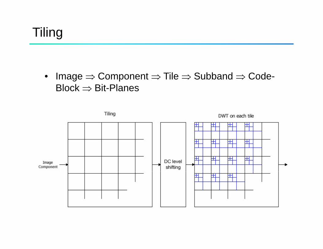
Tiling
• Image ⇒ Component ⇒ Tile ⇒ Subband ⇒ Code-Image ⇒ Component ⇒ Tile ⇒ Subband ⇒ CodeBlock ⇒ Bit-Planes
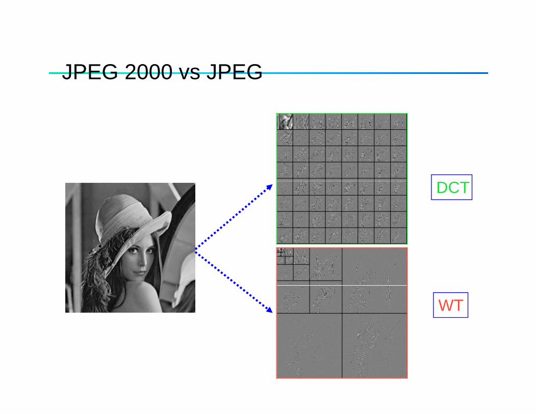
JPEG 2000 vs JPEGJPEG 2000 vs JPEG
DCT
WT
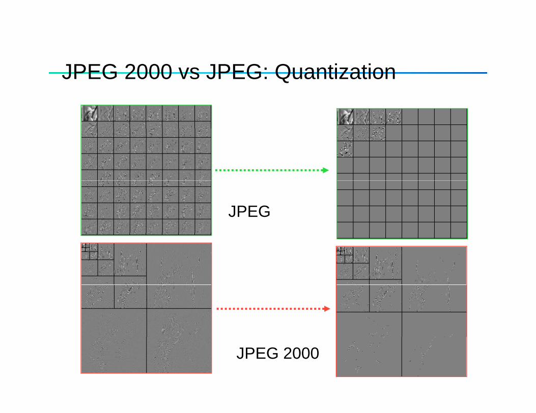
JPEG 2000 vs JPEG: QuantizationJPEG 2000 vs JPEG: Quantization
JPEG
JPEG 2000
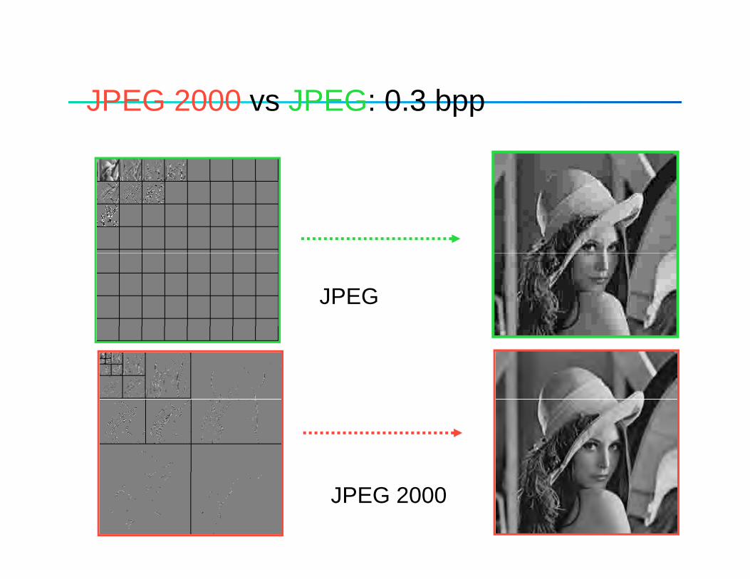
JPEG 2000 vs JPEG: 0 3 bppJPEG 2000 vs JPEG: 0.3 bpp
JPEG
JPEG 2000
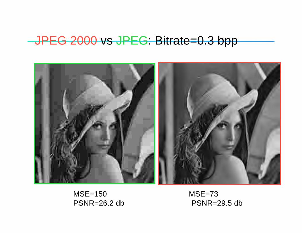
JPEG 2000 vs JPEG: Bitrate=0 3 bppJPEG 2000 vs JPEG: Bitrate 0.3 bpp
MSE=150 MSE=73PSNR=26.2 db PSNR=29.5 db
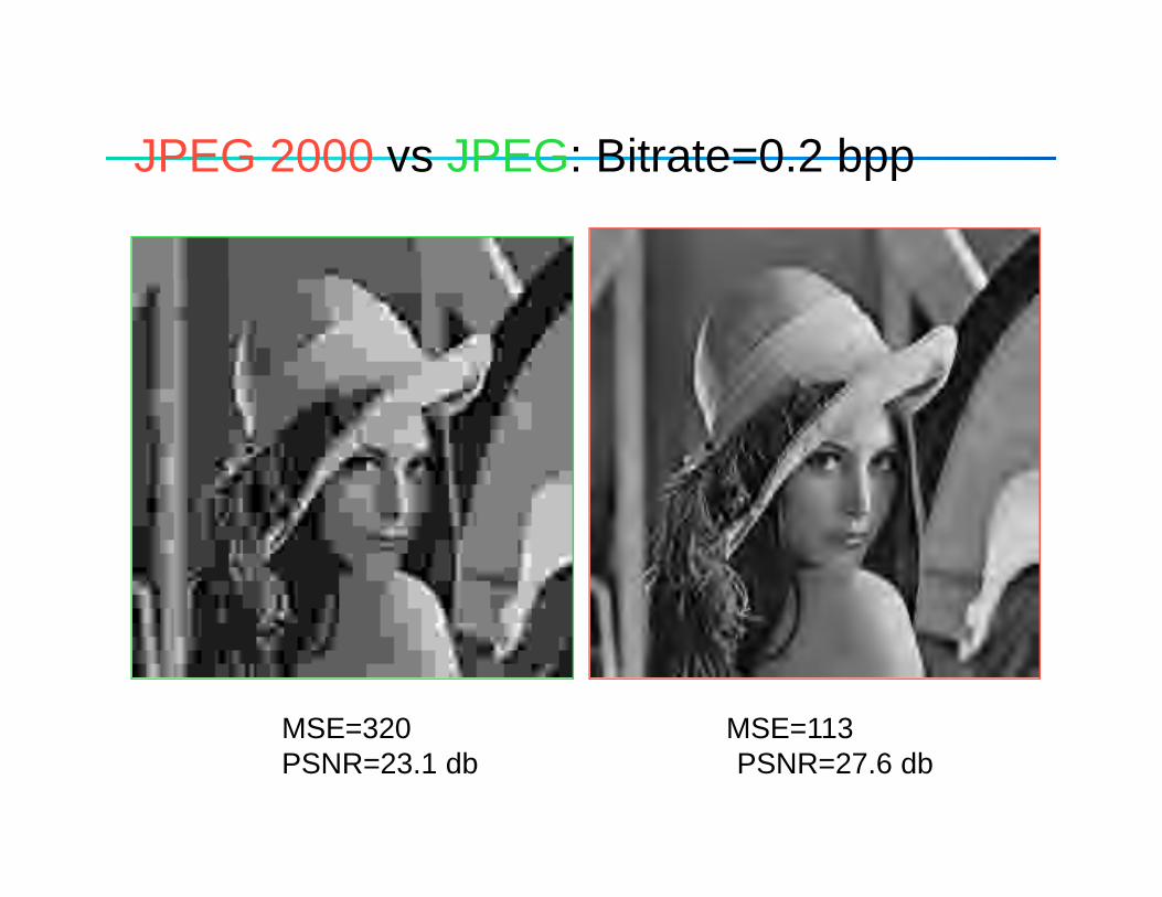
JPEG 2000 vs JPEG: Bitrate=0 2 bppJPEG 2000 vs JPEG: Bitrate 0.2 bpp
MSE=320 MSE=113MSE=320 MSE=113PSNR=23.1 db PSNR=27.6 db
Top Related