


Languages
Pages
Legal

Lap Time Simulation Tool for the Development of an Electric FormulaStudent Car
Doyle, D., Cunningham, G., White, G., & Early, J. (2019). Lap Time Simulation Tool for the Development of anElectric Formula Student Car. In WCX SAE World Congress Experience 2019: Proceedings (SAE TechnicalPapers). SAE International. https://doi.org/10.4271/2019-01-0163
Published in:WCX SAE World Congress Experience 2019: Proceedings
Document Version:Peer reviewed version
Queen's University Belfast - Research Portal:Link to publication record in Queen's University Belfast Research Portal
Publisher rightsCopyright 2019 SAE.This work is made available online in accordance with the publisher’s policies. Please refer to any applicable terms of use of the publisher.
General rightsCopyright for the publications made accessible via the Queen's University Belfast Research Portal is retained by the author(s) and / or othercopyright owners and it is a condition of accessing these publications that users recognise and abide by the legal requirements associatedwith these rights.
Take down policyThe Research Portal is Queen's institutional repository that provides access to Queen's research output. Every effort has been made toensure that content in the Research Portal does not infringe any person's rights, or applicable UK laws. If you discover content in theResearch Portal that you believe breaches copyright or violates any law, please contact [email protected].
Download date:07. Dec. 2021
01/15/2019
2019-01-0163
Lap Time Simulation Tool for the Development of an Electric Formula Student Car Author, co-author (Do NOT enter this information. It will be pulled from participant tab in
MyTechZone) Affiliation (Do NOT enter this information. It will be pulled from participant tab in MyTechZone)
Abstract
This work details the development of a lap time simulation (LTS) tool for use by Queen’s University Belfast in the Formula Student
UK competition. The tool provides an adaptable, user-friendly virtual
test environment for the development of the team’s first electric
vehicle. A vehicle model was created within Simulink, and a series of events simulated to generate the performance envelope of the car in
the form of maximum combined lateral/longitudinal accelerations
against velocity (ggv diagram). A four-wheeled vehicle including
load transfer was modelled, capturing shifts in traction between each tire, which can influence performance in vehicles where the total
tractive power is split between individual wheel motors. The
acceleration limits in the ggv diagram were used to simulate the
acceleration and endurance events at Formula Student. These events were simulated using a MATLAB code considering a point mass,
quasi-steady state model with a perfect driver. This method
considering all four wheels captures performance characteristics that
point mass models normally cannot, without the complexity and time required for more detailed LTS solutions including yaw movements
and driver models. It also separates the vehicle model from the
MATLAB code required to run the LTS, reducing the complexity of
implementing future changes. The LTS was benchmarked against the freeware tool OptimumLap and validated where possible against
competition results. A Latin Hypercube sampling technique was
employed to generate numerous input scenarios for the simulation,
and a response surface fitted to the results to perform a sensitivity
analysis. Results from this analysis indicate several areas to
efficiently focus future resource allocation as well as attempting to
quantify trade-offs. Optimum powertrain gear ratio and battery
capacity for a proposed vehicle were specified using the tool.
Introduction
Formula Student (FS) is an annual competition which “challenges
students to conceive, design, fabricate, and compete with small
formula-style racing cars” [1]. With the competition occurring every
year, teams face issues in the form of rapid development and limited testing time, as well as knowledge loss between subsequent years as
team members leave their university. Teams compete in various
events, the most critical of which for the purposes of this work being
the 75 m acceleration event and the 22 km endurance event. Alongside the rise in popularity of passenger electric vehicles (EVs),
FS has seen an increasing number of EVs competing against internal
combustion engine (ICE) cars each year since their introduction to
the competition in 2012. Queen’s University Belfast (QUB) aim to
compete in the competition with an EV for the first time in 2020 –
with the proposed car featuring four wheel drive in the form of four
individually powered in-hub motors with speed reduction gearing.
Variation of many vehicle design parameters rarely yield a linear or easily predictable change in performance, with many changes
involving trade-offs which must be evaluated. Real world testing is
both expensive and time consuming, and evaluation of new concepts
may require the production of several prototypes. Simulation through a computer-based vehicle model provides a virtual test environment,
allowing the evaluation of new concepts or design decisions to be
done quicker and at a much lower cost. A method of LTS is
particularly useful to QUB due to the short development time available each year for FS and the increased ability to influence
design decisions in the current early stages of development.
Background
Simulation is widely carried out within FS, professional racing and
the commercial automotive industry with varying degrees of
complexity. Driver-in-the-loop simulators have a human driver
provide steering and pedal inputs in order to navigate a track, who
may in turn receive motion feedback and immersive surrounding
graphics. The underlying vehicle models are generally very detailed,
with tire models obtained from test data, yaw motion, transient suspension effects and multibody dynamics. These are widely
adopted in Formula One, with the added benefit of driver training as
well as virtual testing - however testing or comparison between
vehicle models is subject to human variability.
Replacing the human driver with a controller (driver model) allows
LTS to be carried out automatically and consistently, albeit with
additional challenges. The commercial automotive or transport
industries make use of standard drive cycles and program the driver model to follow a specified velocity profile, using bespoke models or
flexible packages such as AVL CRUISE (as in [2]). This is obviously
less useful in LTS for racing where the goal is to maximize the
velocity profile around a track of specified geometry. Non-linear or discontinuous vehicle performance (for example when maximum
velocity is reached) must be accounted for within the driver model.
Packages such as IPG CarMaker have been used for FS applications
[3], which are again generally complex and aimed towards the
detailed design stages.
A simpler method is to model the vehicle as a point mass, single-tire
vehicle, with a constant coefficient of friction tire model. This
removes the necessity of detailed tire models, and reduces complexity by negating yaw motion – the point mass vehicle can neither
oversteer nor understeer and navigates along a specified course only
under the action of combined longitudinal and lateral tire forces.
Using the limits of performance (either traction limited or power
limited) to produce the lateral and longitudinal accelerations
represents a perfect driver, which although non-realistic is consistent
01/15/2019
for each simulation. The assumptions and simplifications employed with this method are at the expense of accuracy, although provide a
comparative estimate between different setups and can be used
without needing comprehensive information or data from the vehicle.
OptimumLap is a free LTS tool featuring a point mass, quasi-steady state model, used by Centro Universitário FEI in [4]. OptimumLap
quote an accuracy of within 10% in their documentation [5], showing
reasonable accuracy for a simple model. However, single tire, point
mass models cannot simulate some characteristics important to the specification of powertrains with four independently powered wheels,
as proposed by QUB. Under acceleration, load transfer causes the
normal force at each tire to change, therefore changing the available
traction. Consider the case where a vehicle moving at an instantaneous velocity has a total available traction power of 100 kW
and four in-hub motors capable of 30 kW each. Under a single tire
model, there is more motor power available than traction power, and
as such 100 kW is transmitted to the road. Now consider 70% of the load shifts to the rear under acceleration. Now, 70 kW of traction is
available at the rear, with only 60 kW of motor power available. Thus
for the same available traction and available motor power, 10 kW less
power is transmitted to the road.
Sakhalkar et al. avoid this by using a longitudinal vehicle model
which includes longitudinal load transfer under acceleration [6]. The
vehicle treats corners as an equivalent straight section with a velocity
restriction and thus reduces the track to a longitudinal problem. However this doesn’t account for the variance in traction between the
left and right tires through lateral load transfer. Additionally, only
constant speed, steady-state cornering is modelled, compared to the
quasi-steady combined cornering and acceleration/braking allowed within OptimumLap. The maximum cornering velocity is a function
of only the tire coefficient of friction and the local track radius. This
does not factor in downforce or the longitudinal tire force required to
maintain constant velocity, which along with quasi-steady state
cornering are considered necessary in a robust LTS tool for QUB.
Scope
The goal of this work was to produce an LTS tool to aid in the
development of the current proposed and future QUB EVs for FS.
The tool had the following aims:
1. Specify optimum transmission ratio and battery pack capacity. 2. Guide future EV development and funding allocation through a
multivariate sensitivity analysis.
3. Completion within the 24 week university calendar.
4. Address the issue of annual knowledge loss through a model which is easily adaptable to future design changes and requires
little understanding of the underlying methodology to use.
This paper details the methodology behind an LTS tool developed
within MATLAB and Simulink which achieves the listed aims. Due to the combination of a short time frame and an absence of available
tire and vehicle data, the development of the LTS tool was
constrained to a point mass quasi-steady state vehicle model. A
method of addressing point mass models’ inability to capture variations in traction under load transfer is implemented and
discussed. OptimumLap was chosen for comparison as it represents a
baseline point mass model without the additional methodology
described in this paper, has proven accuracy and is used and
encouraged within FS. Additionally it is more focused towards the
early concept design stages than more advanced packages.
Powertrain components are sized using the developed LTS tool and a
sensitivity analysis is performed.
Methodology
A longitudinal vehicle model was created within Simulink, including
four separate drivetrains to represent each motor and their mechanical
connection to the wheels. Each motor is capable of delivering different amounts of torque depending on the instantaneous traction
available at the wheel, whilst staying within the 80 kW total power
limit that applies to EVs in the competition [7].
A simple constant friction coefficient tire model was used in the absence of tire test data, with the maximum tire tractive force in the
form of Eq. (1),
𝐹𝑖 = 𝜇𝑁𝑖 (1)
which after compensating for mechanical efficiency losses, translates
to an equivalent traction limited torque at the motor:
𝑇𝑡𝑟𝑎𝑐𝑡𝑖𝑜𝑛,𝑖 = (𝐹𝑖)𝑟𝑛/η𝑚 (2)
The torque available at each motor for acceleration is the minimum of the traction limited torque and the motor limited torque (as defined
in the manufacturer’s datasheet) at that speed:
𝑇𝑖 = min(𝑇𝑡𝑟𝑎𝑐𝑡𝑖𝑜𝑛,𝑖 , 𝑇𝑚𝑜𝑡𝑜𝑟,𝑖) (3)
Resistive forces acting on the vehicle due to rolling resistance and
drag were calculated using Eq. 4 and 5 respectively.
𝐹𝑅𝑅 =𝐶𝑟∑𝑁𝑖
4
𝑖=1
(4)
𝐹𝑑𝑟𝑎𝑔 = 0.5𝜌𝐶𝑑𝐴𝑣𝑥2 (5)
Similarly, the downforce on the vehicle (assumed to be distributed
evenly between each tire for this study) is given by Eq. 6. A negative
lift produces a positive downward force, hence the negative sign at
the beginning of the equation.
𝐹𝑑𝑜𝑤𝑛𝑓𝑜𝑟𝑐𝑒 =−0.5𝜌𝐶𝑙𝐴𝑣𝑥2 (6)
The final loss modelled under acceleration is due to the rotational
inertia of the rotating components in the drivetrain. These can be
represented as an equivalent mass within the translational form of Newton’s 2nd Law, using the method outlined in [8], which in the
reference frame of the vehicle acceleration becomes:
∑ 𝑇𝑖4𝑖=1 𝑛η𝑚
𝑟− 𝐹𝑅𝑅 − 𝐹𝑑𝑟𝑎𝑔 = ⋯
= ((∑ 𝐼𝑈𝑝𝑠𝑡𝑟𝑒𝑎𝑚,𝑖4𝑖=1 . 𝑛2 + ∑ 𝐼𝐷𝑜𝑤𝑛𝑠𝑡𝑟𝑒𝑎𝑚,𝑖
4𝑖=1
𝑟2)+ 𝑚)𝑎𝑥
(7)
The rotational inertia of each drivetrain component was divided into
upstream and downstream of the gear ratio to account the increase in
apparent inertia of upstream components. Using Eq. 7, the
01/15/2019
longitudinal vehicle acceleration can be determined from the applied
motor torques.
The power required from the battery is given by Eq. 8, where the
electrical efficiency represents the efficiency of the motor, inverters,
cables and battery.
𝑃 =∑𝑇𝑖𝜔/𝜂𝑒
4
𝑖=1
(8)
When braking, power is recovered through regenerative braking
within the motors. Additional braking can be provided by friction
brakes if the demanded braking torque exceeds the motor limits.
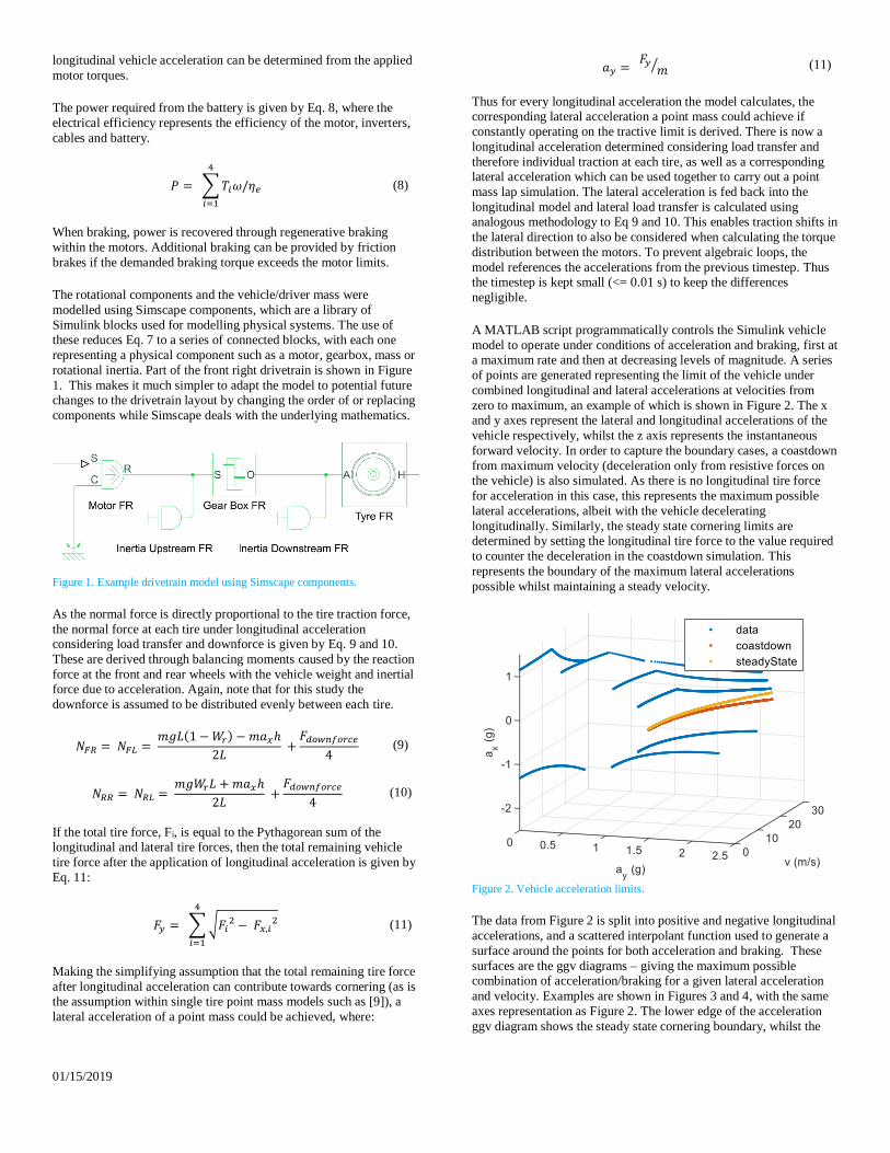
The rotational components and the vehicle/driver mass were
modelled using Simscape components, which are a library of
Simulink blocks used for modelling physical systems. The use of these reduces Eq. 7 to a series of connected blocks, with each one
representing a physical component such as a motor, gearbox, mass or
rotational inertia. Part of the front right drivetrain is shown in Figure
1. This makes it much simpler to adapt the model to potential future changes to the drivetrain layout by changing the order of or replacing
components while Simscape deals with the underlying mathematics.
Figure 1. Example drivetrain model using Simscape components.
As the normal force is directly proportional to the tire traction force,
the normal force at each tire under longitudinal acceleration considering load transfer and downforce is given by Eq. 9 and 10.
These are derived through balancing moments caused by the reaction
force at the front and rear wheels with the vehicle weight and inertial force due to acceleration. Again, note that for this study the
downforce is assumed to be distributed evenly between each tire.
𝑁𝐹𝑅 =𝑁𝐹𝐿 =𝑚𝑔𝐿(1 −𝑊𝑟) − 𝑚𝑎𝑥ℎ
2𝐿+
𝐹𝑑𝑜𝑤𝑛𝑓𝑜𝑟𝑐𝑒
4 (9)
𝑁𝑅𝑅 =𝑁𝑅𝐿 =𝑚𝑔𝑊𝑟𝐿 + 𝑚𝑎𝑥ℎ
2𝐿+
𝐹𝑑𝑜𝑤𝑛𝑓𝑜𝑟𝑐𝑒
4 (10)
If the total tire force, Fi, is equal to the Pythagorean sum of the longitudinal and lateral tire forces, then the total remaining vehicle
tire force after the application of longitudinal acceleration is given by
Eq. 11:
𝐹𝑦 =∑√𝐹𝑖2 −𝐹𝑥,𝑖
2
4
𝑖=1
(11)
Making the simplifying assumption that the total remaining tire force
after longitudinal acceleration can contribute towards cornering (as is
the assumption within single tire point mass models such as [9]), a
lateral acceleration of a point mass could be achieved, where:
𝑎𝑦 =𝐹𝑦
𝑚⁄ (11)
Thus for every longitudinal acceleration the model calculates, the corresponding lateral acceleration a point mass could achieve if
constantly operating on the tractive limit is derived. There is now a
longitudinal acceleration determined considering load transfer and
therefore individual traction at each tire, as well as a corresponding lateral acceleration which can be used together to carry out a point
mass lap simulation. The lateral acceleration is fed back into the
longitudinal model and lateral load transfer is calculated using analogous methodology to Eq 9 and 10. This enables traction shifts in
the lateral direction to also be considered when calculating the torque
distribution between the motors. To prevent algebraic loops, the
model references the accelerations from the previous timestep. Thus the timestep is kept small (<= 0.01 s) to keep the differences
negligible.
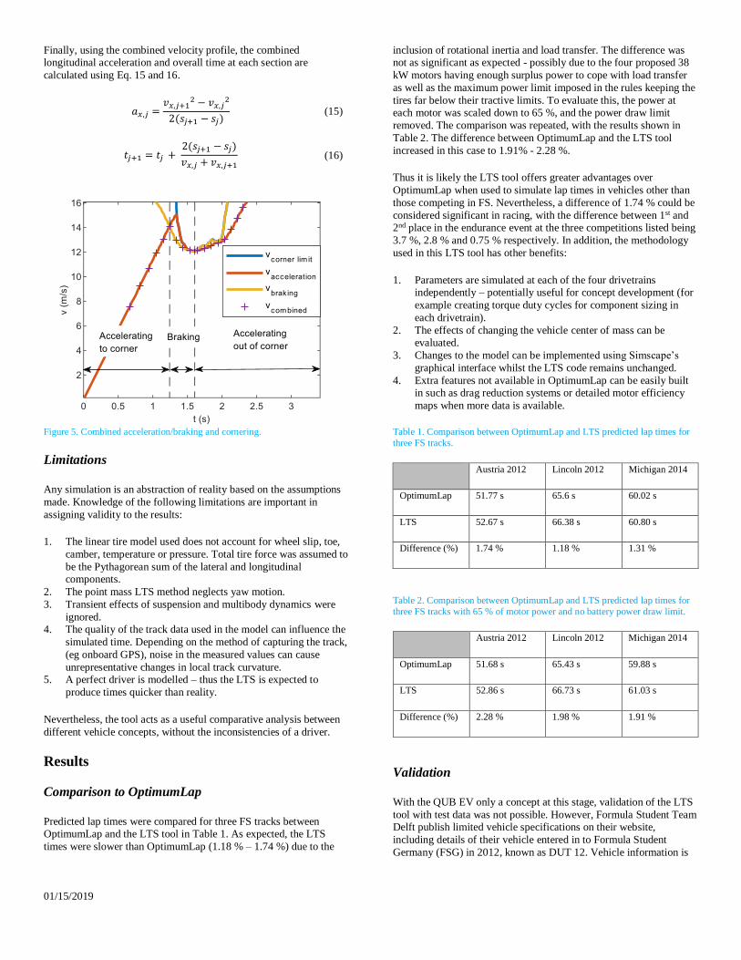
A MATLAB script programmatically controls the Simulink vehicle
model to operate under conditions of acceleration and braking, first at a maximum rate and then at decreasing levels of magnitude. A series
of points are generated representing the limit of the vehicle under
combined longitudinal and lateral accelerations at velocities from
zero to maximum, an example of which is shown in Figure 2. The x and y axes represent the lateral and longitudinal accelerations of the
vehicle respectively, whilst the z axis represents the instantaneous
forward velocity. In order to capture the boundary cases, a coastdown
from maximum velocity (deceleration only from resistive forces on the vehicle) is also simulated. As there is no longitudinal tire force
for acceleration in this case, this represents the maximum possible
lateral accelerations, albeit with the vehicle decelerating
longitudinally. Similarly, the steady state cornering limits are
determined by setting the longitudinal tire force to the value required
to counter the deceleration in the coastdown simulation. This
represents the boundary of the maximum lateral accelerations
possible whilst maintaining a steady velocity.
Figure 2. Vehicle acceleration limits.
The data from Figure 2 is split into positive and negative longitudinal
accelerations, and a scattered interpolant function used to generate a
surface around the points for both acceleration and braking. These
surfaces are the ggv diagrams – giving the maximum possible combination of acceleration/braking for a given lateral acceleration
and velocity. Examples are shown in Figures 3 and 4, with the same
axes representation as Figure 2. The lower edge of the acceleration
ggv diagram shows the steady state cornering boundary, whilst the

01/15/2019
upper edge of the braking ggv diagram shows the coastdown deceleration boundary. The same plots can be created for any chosen
parameter, such as battery power or motor torques. Thus for any
given vehicle acceleration and velocity state the corresponding value
of the chosen parameter is also known.
Sampling the data points from these plots during the lap simulation
enables the performance to represent a perfect driver driving at the
limit of the vehicle, whilst taking into account the limitations in
longitudinal acceleration as a result of load transfer and traction shifts. This method also means that the script used to perform the lap
simulation only requires the ggv diagrams, and is therefore
independent to the vehicle model within Simulink. Changes to the
model or vehicle setup do not require any changes in the MATLAB
code which controls the lap simulation.
Figure 3. Acceleration ggv diagram.
Figure 4. Braking ggv diagram.
Lap Time Simulation
The tracks used for LTS are split into small equidistant sections. The
local curvature, k, is defined for each section, where:
𝑘 =1
𝑅 (12)
The maximum obtainable corner velocity is set for each section as the
steady state cornering limits previously determined. To maintain a curved path, the lateral acceleration is equal to the centripetal
acceleration in Eq. 13.
𝑎𝑦 =𝑣𝑥
2
R= 𝑣𝑥
2𝑘 (13)
Using the limit of the acceleration ggv diagram where ax = 0, the achievable steady state lateral accelerations are found at every
velocity. By rearranging Eq. 13 the maximum curvature possible at
each velocity under steady state cornering is obtained. Thus, given
the local curvature at each track section, a maximum steady state
cornering velocity is set.
Beginning from the first track section, the acceleration ggv diagram
is used to determine the achievable velocities under acceleration. The
velocity entering each section determines the lateral acceleration required to maintain the local curvature using Eq 13. Using the
acceleration ggv diagram as a 2-D lookup table gives the longitudinal
acceleration that can be achieved with the instantaneous velocity and
lateral acceleration. Thus quasi-static, combined acceleration and
cornering is achieved.
Using the equations of motion, the velocity at the end of the track
section is given by Eq 14.
𝑣𝑥,𝑗+1 = 𝑣𝑥,𝑗 + 2𝑎𝑥,𝑗(𝑠𝑗+1 − 𝑠𝑗) (14)
If the velocity at a section exceeds the steady state cornering velocity
limit, then it is reset to the cornering velocity and acceleration begins again in the subsequent sections. This creates the acceleration
velocity profile which indicates the maximum velocity possible at
each section based on the car acceleration limits and maximum
cornering velocities.
However this does not account for the distance required to decelerate
the car to the cornering velocities. By using the same method as
before, but instead starting at the final section of the track and
working in reverse by using the decelerations from the braking ggv
diagram, a braking velocity profile is also created.
By taking the minimum of the acceleration and braking velocity
profiles, the final velocity profile across the lap is generating which
obeys the limits of the vehicle under acceleration, braking and cornering. This is the same as the method used by OptimumLap [5],
with the difference that the accelerations are determined using the
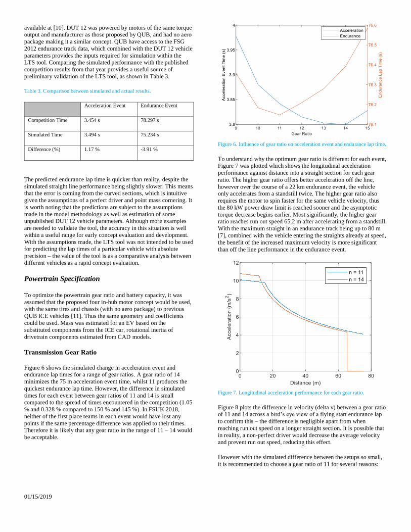
ggv method. Figure 5 shows an example of this at the beginning of a lap. The acceleration velocity profile can be seen to increase at the
limits of the vehicle until the cornering velocity limit is reached, after
which it follows the cornering limit. When the track curvature
decreases causing the corner velocity limit to increase, the acceleration velocity profile increases again at the limit of the
vehicle. Similarly, moving across the plot from right to left, the
braking velocity profile follows the corner speed limit until the track
curvature decreases, allowing it to increase at a magnitude equal to the maximum rate of braking. The intersections between the two
velocity profiles show the transitions from acceleration to braking
and vice versa.
01/15/2019
Finally, using the combined velocity profile, the combined longitudinal acceleration and overall time at each section are
calculated using Eq. 15 and 16.
𝑎𝑥,𝑗 =𝑣𝑥,𝑗+1
2 − 𝑣𝑥,𝑗2
2(𝑠𝑗+1 − 𝑠𝑗) (15)
𝑡𝑗+1 = 𝑡𝑗 +2(𝑠𝑗+1 − 𝑠𝑗)
𝑣𝑥,𝑗 + 𝑣𝑥,𝑗+1 (16)
Figure 5. Combined acceleration/braking and cornering.
Limitations
Any simulation is an abstraction of reality based on the assumptions
made. Knowledge of the following limitations are important in
assigning validity to the results:
1. The linear tire model used does not account for wheel slip, toe,
camber, temperature or pressure. Total tire force was assumed to
be the Pythagorean sum of the lateral and longitudinal components.
2. The point mass LTS method neglects yaw motion.
3. Transient effects of suspension and multibody dynamics were
ignored. 4. The quality of the track data used in the model can influence the
simulated time. Depending on the method of capturing the track,
(eg onboard GPS), noise in the measured values can cause
unrepresentative changes in local track curvature. 5. A perfect driver is modelled – thus the LTS is expected to
produce times quicker than reality.
Nevertheless, the tool acts as a useful comparative analysis between
different vehicle concepts, without the inconsistencies of a driver.
Results
Comparison to OptimumLap
Predicted lap times were compared for three FS tracks between
OptimumLap and the LTS tool in Table 1. As expected, the LTS
times were slower than OptimumLap (1.18 % – 1.74 %) due to the
inclusion of rotational inertia and load transfer. The difference was not as significant as expected - possibly due to the four proposed 38
kW motors having enough surplus power to cope with load transfer
as well as the maximum power limit imposed in the rules keeping the
tires far below their tractive limits. To evaluate this, the power at each motor was scaled down to 65 %, and the power draw limit
removed. The comparison was repeated, with the results shown in
Table 2. The difference between OptimumLap and the LTS tool
increased in this case to 1.91% - 2.28 %.
Thus it is likely the LTS tool offers greater advantages over
OptimumLap when used to simulate lap times in vehicles other than
those competing in FS. Nevertheless, a difference of 1.74 % could be
considered significant in racing, with the difference between 1st and 2nd place in the endurance event at the three competitions listed being
3.7 %, 2.8 % and 0.75 % respectively. In addition, the methodology
used in this LTS tool has other benefits:
1. Parameters are simulated at each of the four drivetrains independently – potentially useful for concept development (for
example creating torque duty cycles for component sizing in
each drivetrain).
2. The effects of changing the vehicle center of mass can be evaluated.
3. Changes to the model can be implemented using Simscape’s
graphical interface whilst the LTS code remains unchanged.
4. Extra features not available in OptimumLap can be easily built in such as drag reduction systems or detailed motor efficiency
maps when more data is available.
Table 1. Comparison between OptimumLap and LTS predicted lap times for
three FS tracks.
Austria 2012 Lincoln 2012 Michigan 2014
OptimumLap 51.77 s 65.6 s 60.02 s
LTS 52.67 s 66.38 s 60.80 s
Difference (%) 1.74 % 1.18 % 1.31 %
Table 2. Comparison between OptimumLap and LTS predicted lap times for
three FS tracks with 65 % of motor power and no battery power draw limit.
Austria 2012 Lincoln 2012 Michigan 2014
OptimumLap 51.68 s 65.43 s 59.88 s
LTS 52.86 s 66.73 s 61.03 s
Difference (%) 2.28 % 1.98 % 1.91 %
Validation
With the QUB EV only a concept at this stage, validation of the LTS
tool with test data was not possible. However, Formula Student Team Delft publish limited vehicle specifications on their website,
including details of their vehicle entered in to Formula Student
Germany (FSG) in 2012, known as DUT 12. Vehicle information is
01/15/2019
available at [10]. DUT 12 was powered by motors of the same torque output and manufacturer as those proposed by QUB, and had no aero
package making it a similar concept. QUB have access to the FSG
2012 endurance track data, which combined with the DUT 12 vehicle
parameters provides the inputs required for simulation within the LTS tool. Comparing the simulated performance with the published
competition results from that year provides a useful source of
preliminary validation of the LTS tool, as shown in Table 3.
Table 3. Comparison between simulated and actual results.
Acceleration Event Endurance Event
Competition Time 3.454 s 78.297 s
Simulated Time 3.494 s 75.234 s
Difference (%) 1.17 % -3.91 %
The predicted endurance lap time is quicker than reality, despite the
simulated straight line performance being slightly slower. This means that the error is coming from the curved sections, which is intuitive
given the assumptions of a perfect driver and point mass cornering. It
is worth noting that the predictions are subject to the assumptions
made in the model methodology as well as estimation of some unpublished DUT 12 vehicle parameters. Although more examples
are needed to validate the tool, the accuracy in this situation is well
within a useful range for early concept evaluation and development.
With the assumptions made, the LTS tool was not intended to be used
for predicting the lap times of a particular vehicle with absolute
precision – the value of the tool is as a comparative analysis between
different vehicles as a rapid concept evaluation.
Powertrain Specification
To optimize the powertrain gear ratio and battery capacity, it was
assumed that the proposed four in-hub motor concept would be used, with the same tires and chassis (with no aero package) to previous
QUB ICE vehicles [11]. Thus the same geometry and coefficients
could be used. Mass was estimated for an EV based on the
substituted components from the ICE car, rotational inertia of
drivetrain components estimated from CAD models.
Transmission Gear Ratio
Figure 6 shows the simulated change in acceleration event and endurance lap times for a range of gear ratios. A gear ratio of 14
minimizes the 75 m acceleration event time, whilst 11 produces the
quickest endurance lap time. However, the difference in simulated
times for each event between gear ratios of 11 and 14 is small compared to the spread of times encountered in the competition (1.05
% and 0.328 % compared to 150 % and 145 %). In FSUK 2018,
neither of the first place teams in each event would have lost any
points if the same percentage difference was applied to their times. Therefore it is likely that any gear ratio in the range of 11 – 14 would
be acceptable.
Figure 6. Influence of gear ratio on acceleration event and endurance lap time.
To understand why the optimum gear ratio is different for each event, Figure 7 was plotted which shows the longitudinal acceleration
performance against distance into a straight section for each gear
ratio. The higher gear ratio offers better acceleration off the line,
however over the course of a 22 km endurance event, the vehicle only accelerates from a standstill twice. The higher gear ratio also
requires the motor to spin faster for the same vehicle velocity, thus
the 80 kW power draw limit is reached sooner and the asymptotic
torque decrease begins earlier. Most significantly, the higher gear ratio reaches run out speed 65.2 m after accelerating from a standstill.
With the maximum straight in an endurance track being up to 80 m
[7], combined with the vehicle entering the straights already at speed,
the benefit of the increased maximum velocity is more significant
than off the line performance in the endurance event.
Figure 7. Longitudinal acceleration performance for each gear ratio.
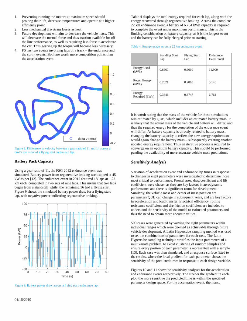
Figure 8 plots the difference in velocity (delta v) between a gear ratio of 11 and 14 across a bird’s eye view of a flying start endurance lap
to confirm this – the difference is negligible apart from when
reaching run out speed on a longer straight section. It is possible that
in reality, a non-perfect driver would decrease the average velocity
and prevent run out speed, reducing this effect.
However with the simulated difference between the setups so small,
it is recommended to choose a gear ratio of 11 for several reasons:
01/15/2019
1. Preventing running the motors at maximum speed should prolong their life, decrease temperatures and operate at a higher
efficiency point.
2. Less mechanical drivetrain losses as heat.
3. Future development will aim to decrease the vehicle mass. This will decrease the normal force and thus traction available for off
the line performance, as well as requiring less force to accelerate
the car. Thus gearing up the torque will become less necessary.
4. FS has two events involving laps of a track – the endurance and the sprint events. Both are worth more competition points than
the acceleration event.
Figure 8. Difference in velocity between a gear ratio of 11 and 14 across a
bird’s eye view of a flying start endurance lap.
Battery Pack Capacity
Using a gear ratio of 11, the FSG 2012 endurance event was
simulated. Battery power from regenerative braking was capped at 45 kW as per [12]. The endurance event in 2012 featured 18 laps at 1.22
km each, completed in two sets of nine laps. This means that two laps
began from a standstill, whilst the remaining 16 had a flying start.
Figure 9 shows the simulated battery power draw for a flying start lap, with negative power indicating regenerative braking.
Figure 9. Battery power draw across a flying start endurance lap.
Table 4 displays the total energy required for each lap, along with the energy recovered through regenerative braking. Across the complete
22 km endurance event, a battery of 6.764 kWh capacity is required
to complete the event under maximum performance. This is the
limiting consideration on battery capacity, as it is the longest event
and the battery can be fully charged prior to starting.
Table 4. Energy usage across a 22 km endurance event.
Standing Start
Lap
Flying Start
Lap
Endurance
Event Total
Energy Used
(kWh) 0.6667 0.6610 11.909
Regen Energy
(kWh) 0.2821 0.2863 5.145
Energy
Required (kWh) 0.3846 0.3747 6.764
It is worth noting that the mass of the vehicle for these simulations
was estimated by QUB, which includes an estimated battery mass. It
is likely that the actual mass of the vehicle and battery will differ, and
thus the required energy for the completion of the endurance event will differ. As battery capacity is directly related to battery mass,
changing the battery capacity to reflect the new energy requirement
would again change the battery mass – subsequently creating another
updated energy requirement. Thus an iterative process is required to converge on an optimum battery capacity. This should be performed
pending the availability of more accurate vehicle mass predictions.
Sensitivity Analysis
Variation of acceleration event and endurance lap times in response
to changes in eight parameters were investigated to determine those
most critical to performance. Frontal area, drag coefficient and lift coefficient were chosen as they are key factors in aerodynamic
performance and there is significant room for development.
Similarly, the vehicle mass and center of mass position are
parameters QUB can change in subsequent years, and are key factors in acceleration and load transfer. Electrical efficiency, rolling
resistance coefficient and tire friction coefficient are included to
understand the sensitivity of the model to estimated parameters and
thus the need to obtain more accurate values.
500 cases were generated by varying the eight parameters within
individual ranges which were deemed as achievable through future
vehicle development. A Latin Hypercube sampling method was used
to set the combinations of parameters for each case. The Latin Hypercube sampling technique stratifies the input parameters of a
multivariate problem, to avoid clustering of random samples and
ensure every portion of each parameter is represented with a sample
[13]. Each case was then simulated, and a response surface fitted to the results, where the local gradient for each parameter shows the
sensitivity of the predicted times in response to each design variable.
Figures 10 and 11 show the sensitivity analyses for the acceleration
and endurance events respectively. The steeper the gradient in each
plot, the more sensitive the predicted time is within the specified
parameter design space. For the acceleration event, the mass,
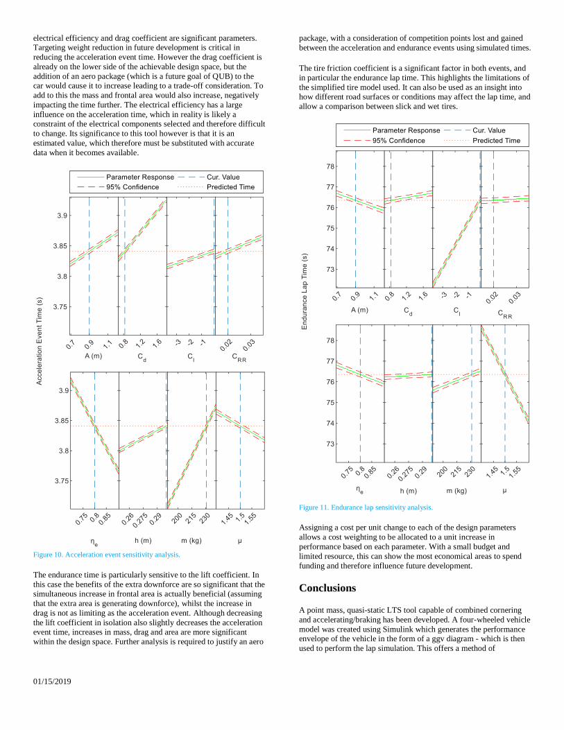
01/15/2019
electrical efficiency and drag coefficient are significant parameters. Targeting weight reduction in future development is critical in
reducing the acceleration event time. However the drag coefficient is
already on the lower side of the achievable design space, but the
addition of an aero package (which is a future goal of QUB) to the car would cause it to increase leading to a trade-off consideration. To
add to this the mass and frontal area would also increase, negatively
impacting the time further. The electrical efficiency has a large
influence on the acceleration time, which in reality is likely a constraint of the electrical components selected and therefore difficult
to change. Its significance to this tool however is that it is an
estimated value, which therefore must be substituted with accurate
data when it becomes available.
Figure 10. Acceleration event sensitivity analysis.
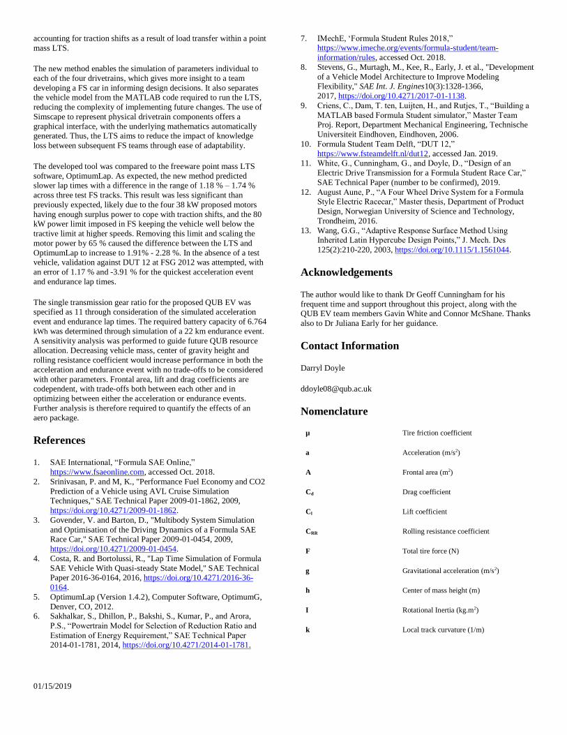
The endurance time is particularly sensitive to the lift coefficient. In
this case the benefits of the extra downforce are so significant that the simultaneous increase in frontal area is actually beneficial (assuming
that the extra area is generating downforce), whilst the increase in
drag is not as limiting as the acceleration event. Although decreasing
the lift coefficient in isolation also slightly decreases the acceleration event time, increases in mass, drag and area are more significant
within the design space. Further analysis is required to justify an aero
package, with a consideration of competition points lost and gained
between the acceleration and endurance events using simulated times.
The tire friction coefficient is a significant factor in both events, and
in particular the endurance lap time. This highlights the limitations of
the simplified tire model used. It can also be used as an insight into how different road surfaces or conditions may affect the lap time, and
allow a comparison between slick and wet tires.
Figure 11. Endurance lap sensitivity analysis.
Assigning a cost per unit change to each of the design parameters
allows a cost weighting to be allocated to a unit increase in
performance based on each parameter. With a small budget and
limited resource, this can show the most economical areas to spend
funding and therefore influence future development.
Conclusions
A point mass, quasi-static LTS tool capable of combined cornering
and accelerating/braking has been developed. A four-wheeled vehicle
model was created using Simulink which generates the performance envelope of the vehicle in the form of a ggv diagram - which is then
used to perform the lap simulation. This offers a method of
01/15/2019
accounting for traction shifts as a result of load transfer within a point
mass LTS.
The new method enables the simulation of parameters individual to
each of the four drivetrains, which gives more insight to a team
developing a FS car in informing design decisions. It also separates the vehicle model from the MATLAB code required to run the LTS,
reducing the complexity of implementing future changes. The use of
Simscape to represent physical drivetrain components offers a
graphical interface, with the underlying mathematics automatically generated. Thus, the LTS aims to reduce the impact of knowledge
loss between subsequent FS teams through ease of adaptability.
The developed tool was compared to the freeware point mass LTS
software, OptimumLap. As expected, the new method predicted slower lap times with a difference in the range of 1.18 % – 1.74 %
across three test FS tracks. This result was less significant than
previously expected, likely due to the four 38 kW proposed motors
having enough surplus power to cope with traction shifts, and the 80 kW power limit imposed in FS keeping the vehicle well below the
tractive limit at higher speeds. Removing this limit and scaling the
motor power by 65 % caused the difference between the LTS and
OptimumLap to increase to 1.91% - 2.28 %. In the absence of a test vehicle, validation against DUT 12 at FSG 2012 was attempted, with
an error of 1.17 % and -3.91 % for the quickest acceleration event
and endurance lap times.
The single transmission gear ratio for the proposed QUB EV was specified as 11 through consideration of the simulated acceleration
event and endurance lap times. The required battery capacity of 6.764
kWh was determined through simulation of a 22 km endurance event.
A sensitivity analysis was performed to guide future QUB resource allocation. Decreasing vehicle mass, center of gravity height and
rolling resistance coefficient would increase performance in both the
acceleration and endurance event with no trade-offs to be considered
with other parameters. Frontal area, lift and drag coefficients are codependent, with trade-offs both between each other and in
optimizing between either the acceleration or endurance events.
Further analysis is therefore required to quantify the effects of an
aero package.
References
1. SAE International, “Formula SAE Online,”
https://www.fsaeonline.com, accessed Oct. 2018.
2. Srinivasan, P. and M, K., "Performance Fuel Economy and CO2
Prediction of a Vehicle using AVL Cruise Simulation Techniques," SAE Technical Paper 2009-01-1862, 2009,
https://doi.org/10.4271/2009-01-1862.
3. Govender, V. and Barton, D., "Multibody System Simulation
and Optimisation of the Driving Dynamics of a Formula SAE
Race Car," SAE Technical Paper 2009-01-0454, 2009,
https://doi.org/10.4271/2009-01-0454.
4. Costa, R. and Bortolussi, R., "Lap Time Simulation of Formula
SAE Vehicle With Quasi-steady State Model," SAE Technical Paper 2016-36-0164, 2016, https://doi.org/10.4271/2016-36-
0164.
5. OptimumLap (Version 1.4.2), Computer Software, OptimumG,
Denver, CO, 2012. 6. Sakhalkar, S., Dhillon, P., Bakshi, S., Kumar, P., and Arora,
P.S., “Powertrain Model for Selection of Reduction Ratio and
Estimation of Energy Requirement,” SAE Technical Paper 2014-01-1781, 2014, https://doi.org/10.4271/2014-01-1781.
7. IMechE, ‘Formula Student Rules 2018,” https://www.imeche.org/events/formula-student/team-
information/rules, accessed Oct. 2018.
8. Stevens, G., Murtagh, M., Kee, R., Early, J. et al., "Development
of a Vehicle Model Architecture to Improve Modeling Flexibility," SAE Int. J. Engines10(3):1328-1366,
2017, https://doi.org/10.4271/2017-01-1138.
9. Criens, C., Dam, T. ten, Luijten, H., and Rutjes, T., “Building a
MATLAB based Formula Student simulator,” Master Team Proj. Report, Department Mechanical Engineering, Technische
Universiteit Eindhoven, Eindhoven, 2006.
10. Formula Student Team Delft, “DUT 12,”
https://www.fsteamdelft.nl/dut12, accessed Jan. 2019. 11. White, G., Cunningham, G., and Doyle, D., “Design of an
Electric Drive Transmission for a Formula Student Race Car,”
SAE Technical Paper (number to be confirmed), 2019.
12. August Aune, P., “A Four Wheel Drive System for a Formula Style Electric Racecar,” Master thesis, Department of Product
Design, Norwegian University of Science and Technology,
Trondheim, 2016.
13. Wang, G.G., “Adaptive Response Surface Method Using Inherited Latin Hypercube Design Points,” J. Mech. Des
125(2):210-220, 2003, https://doi.org/10.1115/1.1561044.
Acknowledgements
The author would like to thank Dr Geoff Cunningham for his
frequent time and support throughout this project, along with the QUB EV team members Gavin White and Connor McShane. Thanks
also to Dr Juliana Early for her guidance.
Contact Information
Darryl Doyle
Nomenclature
µ Tire friction coefficient
a Acceleration (m/s2)
A Frontal area (m2)
Cd Drag coefficient
Cl Lift coefficient
CRR Rolling resistance coefficient
F Total tire force (N)
g Gravitational acceleration (m/s2)
h Center of mass height (m)
I Rotational Inertia (kg.m2)
k Local track curvature (1/m)
01/15/2019
L Vehicle wheelbase (m)
m Vehicle and driver mass (kg)
n Gear ratio
N Tire normal force (N)
P Power (W)
r Tire rolling radius (m)
R Local track radius (m)
s Displacement (m)
t Time (s)
T Motor torque (Nm)
v Velocity (m/s)
Wr Rear weight distribution (%)
η Efficiency (%)
ρ Air density (kg/m2)
ω Motor angular velocity (rad/s)
Subscripts
e Electrical
i Motor/tire identication (1 = FR,
2 = FL, 3 = RR, 4 = RL)
j Track section
m Mechanical
motor Motor limited
RR Rolling resistance
traction Traction limited
x Longitudinal direction
y Lateral direction
Definitions/Abbreviations
DUT 12 Delft University of Technology
2012
EV Electric Vehicle
FL Front Left
FR Front right
FS Formula Student
FSG Formula Student Germany
FSUK Formula Student United
Kingdom
ICE Internal Combustion Engine
LTS Lap time simulation
QUB Queen’s University Belfast
RL Real Left
RR Rear Right
Top Related