


Languages
Pages
Legal

Air Force Institute of TechnologyAFIT Scholar
Theses and Dissertations Student Graduate Works
3-22-2012
LADAR Performance Simulations with a HighSpectral Resolution Atmospheric Transmittanceand Radiance Model- LEEDRBenjamin D. Roth
Follow this and additional works at: https://scholar.afit.edu/etd
Part of the Atmospheric Sciences Commons, and the Electromagnetics and Photonics Commons
This Thesis is brought to you for free and open access by the Student Graduate Works at AFIT Scholar. It has been accepted for inclusion in Theses andDissertations by an authorized administrator of AFIT Scholar. For more information, please contact [email protected].
Recommended CitationRoth, Benjamin D., "LADAR Performance Simulations with a High Spectral Resolution Atmospheric Transmittance and RadianceModel- LEEDR" (2012). Theses and Dissertations. 1062.https://scholar.afit.edu/etd/1062

LADAR PERFORMANCE SIMULATIONS WITH A HIGH SPECTRAL
RESOLUTION ATMOSPHERIC TRANSMITTANCE AND RADIANCE
MODEL- LEEDR
THESIS
Benjamin D. Roth, Captain, USAF
AFIT/APPLPHY/ENP/12-M09
DEPARTMENT OF THE AIR FORCE AIR UNIVERSITY
AIR FORCE INSTITUTE OF TECHNOLOGY
Wright-Patterson Air Force Base, Ohio
DISTRIBUTION STATEMENT A.
APPROVED FOR PUBLIC RELEASE; DISTRIBUTION UNLIMITED

The views expressed in this thesis are those of the author and do not reflect the official policy or position of the United States Air Force, Department of Defense, or the United States Government. This material is declared a work of the U.S. Government and is not subject to copyright protection in the United States.

AFIT/APPLPHYS/ENP/12-M09
LADAR PERFORMANCE SIMULATIONS WITH A HIGH SPECTRAL
RESOLUTION ATMOSPHERIC TRANSMITTANCE AND RADIANCE
MODEL- LEEDR
THESIS
Presented to the Faculty
Department of Engineering Physics
Graduate School of Engineering and Management
Air Force Institute of Technology
Air University
Air Education and Training Command
In Partial Fulfillment of the Requirements for the
Degree of Master of Science in Applied Physics
Benjamin D. Roth, BS
Captain, USAF
March 2012
DISTRIBUTION STATEMENT A. APPROVED FOR PUBLIC RELEASE; DISTRIBUTION UNLIMITED

AFIT/ APPLPHYS /ENP/12-M09
LADAR PERFORMANCE SIMULATIONS WITH A HIGH SPECTRAL
RESOLUTION ATMOSPHERIC TRANSMITTANCE AND RADIANCE
MODEL- LEEDR
Benjamin D. Roth, BS Captain, USAF
Approved: ___________________________________ _____________ Steven T. Fiorino, PhD (Chairman) Date ___________________________________ _____________ Michael A. Marciniak, PhD (Member) Date ___________________________________ _____________ Kevin C. Gross, PhD (Member) Date ___________________________________ _____________ Paul F. McManamon, PhD (Member) Date

iv
AFIT/ APPLPHYS /ENP/12-M09 Abstract
In this study of atmospheric effects on Geiger Mode laser ranging and detection
(LADAR), the parameter space is explored primarily using the Air Force Institute of
Technology Center for Directed Energy’s (AFIT/CDE) Laser Environmental Effects
Definition and Reference (LEEDR) code. The expected performance of LADAR systems
is assessed at operationally representative wavelengths of 1.064, 1.56 and 2.039 µm at a
number of locations worldwide. Signal attenuation and background noise are
characterized using LEEDR. These results are compared to standard atmosphere and
Fast Atmospheric Signature Code (FASCODE) assessments. Scenarios evaluated are
based on air-to-ground engagements including both down looking oblique and vertical
geometries in which anticipated clear air aerosols are expected to occur. Engagement
geometry variations are considered to determine optimum employment techniques to
exploit or defeat the environmental conditions. Results, presented primarily in the form
of worldwide plots of notional signal to noise ratios, show a significant climate
dependence, but large variances between climatological and standard atmosphere
assessments. An overall average absolute mean difference ratio of 1.03 is found when
climatological signal-to-noise ratios at 40 locations are compared to their equivalent
standard atmosphere assessment. Atmospheric transmission is shown to not always
correlate with signal-to-noise ratios between different atmosphere profiles. Allowing
aerosols to swell with relative humidity proves to be significant especially for up looking
geometries reducing the signal-to-noise ratio several orders of magnitude. Turbulence
blurring effects that impact tracking and imaging show that the LADAR system has little
capability at a 50km range yet the turbulence has little impact at a 3km range.

v
Acknowledgments
I would like to express my appreciation to my faculty advisor, Dr. Steven Fiorino,
for his guidance, support and enthusiasm. He provided guidance at crucial periods during
this effort. I would also like to thank my committee members Dr. Michael Marciniak,
Dr. Kevin Gross, and Dr. Paul McManamon who provided invaluable feedback. A non-
committee advisor, Dr. Jack McCrae joined AFIT and began to assist me at the most
critical point in my thesis effort. His invaluable knowledge and expertise in atmospheric
science and LADAR technologies was greatly appreciated. I am grateful for the help
received from my fellow physics peers. I would also like to thank Mr. Robin Ritter from
Tau Technologies, and Mr. Douglas Jameson from the Air Force Research Laboratory for
answering my myriad of emails.
I am grateful to my father for teaching me the importance of an enduring work
ethic. His faith in me has instilled a knowledge that I can accomplish anything I set my
mind to. I am indebted to my mother, whose endless love and service has made my life
possible. Most of all, I am especially grateful for the love and patience of my wife who
sustained me with a positive attitude through the late nights and stressful moments. May
every moment together be cherished as we experience life together as a family.
Benjamin D. Roth

vi
TableofContents
Page
Abstract .............................................................................................................................. iv
Acknowledgments................................................................................................................v
Table of Contents ............................................................................................................... vi
List of Figures .................................................................................................................. viii
List of Tables ..................................................................................................................... xi
I Introduction ..................................................................................................................1
1.1 Background ........................................................................................................1 1.2 Problem Statement .............................................................................................3 1.3 Purpose ..............................................................................................................4 1.4 Hypothesis .........................................................................................................4 1.5 Approach ...........................................................................................................5 1.6 Implications .......................................................................................................7 1.7 Outline ...............................................................................................................7
II Literature Review .........................................................................................................9
2.1 Chapter Overview ..............................................................................................9 2.2 Relevant Science ................................................................................................9 2.2.1 Atmospheric Effects .......................................................................................9 2.2.2 LADAR Systems ...........................................................................................15 2.3 Relevant Research ...........................................................................................20 2.3.1 Modeling ......................................................................................................20 2.3.2 Previous Research .......................................................................................24 2.4 Summary ..........................................................................................................29
III Methodology ..............................................................................................................30
3.1 Chapter Overview ............................................................................................30 3.2 Tools Used .......................................................................................................33 3.2.1 Laser Environmental Effects Definition and Reference (LEEDR) ..............33 3.2.2 High Energy Laser End-to-End Operational Simulation (HELEEOS) .......34 3.2.3 Phillips Laboratory ExPERT User Software (PLEXUS) .............................35 3.2.4 High Energy Laser System End-to-End Model (HELSEEM) ......................36 3.2.5 Light-Tunneling within WaveTrain ..............................................................37 3.3 Signal Calculations ..........................................................................................38 3.4 Noise Calculations ...........................................................................................41

vii
Page
3.4.1 Laser Scatter Noise ......................................................................................46 3.4.2 Solar Scatter Noise ......................................................................................50 3.4.3 Solar Reflection Noise..................................................................................52 3.4.4 Blackbody Noise...........................................................................................53 3.5 HELSEEM Images ..........................................................................................54 3.6 Summary ..........................................................................................................57
IV Analysis and Results ..................................................................................................58
4.1 Chapter Overview ............................................................................................58 4.2 Results .............................................................................................................58 4.2.1 World Wide Lambertian Target Signal-to-Noise Results ............................58 4.2.1 Signal-to-Noise HELSEEM Image Results ..................................................76 4.3 Summary ..........................................................................................................84
V Conclusions and Recommendations ...........................................................................86
5.1 Chapter Overview ............................................................................................86 5.2 Conclusions of Research .................................................................................86 5.3 Significance of Research .................................................................................88 5.4 Recommendations for Future Research ...........................................................89 5.5 Summary ..........................................................................................................91
Appendix A ........................................................................................................................92
Bibliography ....................................................................................................................104

viii
List of Figures
Figure Page
1. Transmittance due to top molecular absorbers in the atmosphere (Petty 2006) .......................................................................................................................... 11 2. Theoretical contribution of backscatter intensity and frequency spread (Fujii and Fukuchi 2005). ........................................................................................... 14 3. Example of increased attenuation at top of boundary layer due to swollen aerosols. Left is output from LEEDR, right is a LIDAR measurement (Fiorino et al. 2008). .................................................................................................. 22 4. LEEDR inputs screen ................................................................................................... 34 5. A few of the PLEXUS input screens and the output screen with a transmission and radiance plot ................................................................................... 36 6. Image outputs from HELSEEM. From left to right the images are, the beam spread in green and the field of view in yellow at the RPA, the Gaussian beam spot at the target, and last is the return signature of the RPA. ........................................................................................................................... 37 7. Irradiance values for each bin with the target irradiance at the zero bin represented by an asterisk. The ExPERT Shanghai 10 km slant path simulation, solid blue line and the standard urban atmosphere values, red dashed line values are displayed. ......................................................................... 43 8. Probability of detection, solid lines, and probability of false alarm, dashed lines as a function of total number of photons for various signal-to-noise ratios. ................................................................................................. 45 9. Peak probability of detection, solid line and probability of false alarm, dashed line, as a function of the signal to noise ratio. ................................................ 46 10. From left to right, top to bottom, molecular phase function, aerosol phase function, molecular volume scattering coefficient, and the aerosol volume scattering coefficient. .................................................................................... 48 11. The back scattered laser irradiance as a function of the fraction of the beam gated in front of the target. ............................................................................... 50 12. Spectral irradiance at the top of the atmosphere (ASTM 2000) ................................ 51
ix
Figure Page
13. Solar transmittance as a function of sun zenith angle for the summer 1500-1800 50th humidity percentile LEEDR ExPERT atmosphere at Bucharest, Romania ................................................................................................... 53 14. Black body curves for temperatures between 200 and 300 K (Petty 2006). ......................................................................................................................... 54 15. Progression of adding noise from left to right, top to bottom, the sun reflection, pristine image, background and transmission, solar scatter, laser backscatter, and finally the turbulence is added. ............................................... 57 16. Short range slant path and vertical path signal-to-noise ratios for LEEDR ExPERT site atmospheres with GADS aerosols. The platform is at 1530 m altitude looking down at a target on the ground. ................................... 59 17. Long range slant path and vertical path signal-to-noise ratios for LEEDR ExPERT site atmospheres with GADS aerosols. The platform is at 10 km altitude looking down at a target on the ground. ..................................... 61 18. Signal-to-noise ratio correlation at 2.039 μm wavelength 3 km range for the Mid-Latitude North urban simulations. From left to right is the signal, noise, and signal-to-noise plotted against transmission. The x marks the standard profile value and the o marks the FASCODE value. .................. 72 19. Signal-to-noise ratio correlation at 1.56 μm wavelength 3 km range for desert simulations. From left to right is the signal, noise, and signal-to-noise plotted against transmission. The x marks the standard profile value and the o marks the FASCODE value. ................................................. 73 20. Atmosphere profiles for mid-latitude north with urban aerosols, top, and Paris, France ExPERT site, bottom. The columns from left to right are for the different wavelengths, 1.0642 μm, 1.56 μm, and 2.039 μm respectively. ............................................................................................................... 76 21. Short range 3 km slant path image signal-to-noise ratios. The platform is on the ground looking up at a 1530 m altitude target. ............................................ 78 22. Long range 50 km slant path image signal-to-noise ratios. The platform is on the ground looking up at a 10 km altitude target. ............................... 81

x
Figure Page
23. Atmosphere profiles for Shanghai ExPERT with GADS aerosols, Shanghai ExPERT with urban aerosols, and mid-latitude north with urban aerosols from top to bottom. The columns left to right are for the three wavelengths, 1.0642 μm, 1.56 μm, and 2.039 μm respectively. The plots have the extinction coefficient values (km-1) along the x axis and altitude (m) along the y axis. ............................................................................... 83 24. ExPERT with GADS images with atmospheric turbulence effects. Top row is the 3 km slant path engagement while the bottom row is the 50 km slant path engagement. From left to right the columns are for the 1.0642 μm, 1.56 μm, and the 2.039 μm wavelength respectively. ............................. 84

xi
List of Tables
Table Page
1. HELSEEM input parameters and values used in this study. ....................................... 37 2. FASCODE transmissions for the different geometries, wavelengths and various aerosol types .................................................................................................. 62 3. Mid-Latitude North standard atmosphere with MODTRAN urban aerosols for the short range slant and vertical path .................................................... 64 4. Composition of noise components for 1.0642 μm Mid-Latitude North standard atmosphere with MODTRAN urban aerosols (W/m2) ................................ 66 5. Mid-Latitude North standard atmosphere with MODTRAN rural aerosols for the short range slant and vertical path .................................................................. 67 6. Desert standard atmosphere with desert aerosols for the short range slant and vertical path ......................................................................................................... 67 7. Tropical standard atmosphere with maritime tropical aerosols for the short range slant and vertical path .............................................................................. 68 8. Mid-Latitude North standard atmosphere with MODTRAN urban aerosols for the long range slant and vertical path ..................................................... 68 9. Mid-Latitude North standard atmosphere with MODTRAN rural aerosols for the long range slant and vertical path ................................................................... 69 10. Desert standard atmosphere with Desert aerosols for the long range slant and vertical path ......................................................................................................... 69 11. Tropical standard atmosphere with maritime tropical aerosols for the long range slant and vertical path ............................................................................... 70 12. North standard atmosphere with MODTRAN urban aerosols for the short range slant and vertical path ...................................................................................... 74 13. North standard atmosphere with MODTRAN urban aerosols for the long range slant and vertical path ....................................................................................... 75 14. Composition of noise components for the 3 km slant path geometry........................ 79 15. Composition of noise components for the 50 km slant path geometry...................... 82

1
LADAR PERFORMANCE SIMULATIONS WITH A HIGH SPECTRAL
RESOLUTION ATMOSPHERIC TRANSMITTANCE AND RADIANCE
MODEL- LEEDR
I Introduction
1.1 Background
LADAR (Laser Detection and Ranging) systems use the same basic principle of
transmitting and receiving electromagnetic energy of that of RADAR (Radio Detection
and Ranging). The major difference between these systems is that they operate at
different wavelengths. While LADAR is unable to provide the wide area surveillance
which RADAR offers, LADAR signals return much more information because of their
small wavelengths. Radar image resolution is proportional to the frequency and in fact,
3D images can be produced at LADAR wavelengths. The application of LADAR
systems is a growing area of research with current and proposed uses ranging from
robotic vehicle maneuvering to identifying re-entry vehicles for missile defense (Kenyon
2002). The Air Force has a vested interest in this technology because of LADAR's
unique capabilities and implications for Information Surveillance and Reconnaissance
(ISR) missions.
Every system has capabilities and limitations; exploiting those capabilities while
minimizing the limitations is the primary goal of current LADAR system performance
computer modeling efforts. Operational capability of these systems is largely dependent

2
upon propagation through the atmosphere and atmospheric noise sources. Being able to
accurately model atmospheric effects and the resulting signal-to-noise ratio is paramount
in understanding LADAR capabilities as well as identifying areas of further research.
Atmosphere Transmittance studies have routinely been done using Fast
Atmospheric Signature Code (FASCODE) which can incorporate standard and
homogeneous atmosphere profiles. A unique atmosphere propagation and
characterization package called the Laser Environmental Effects Definition and
Reference (LEEDR) has been developed by the Air Force Institute of Technology, Center
for Directed Energy (AFIT/CDE) as part of the High Energy Laser End-to-End
Operational Simulation (HELEEOS) model. LEEDR is a more up-to-date line-by-line
simulation with more realistic atmosphere profiles. The uniqueness of the LEEDR model
is that it incorporates a correlated, probabilistic climatological database that creates
realistic atmosphere profiles (Fiorino et al. 2008). Throughout this study, "LEEDR
profiles" refers to atmospheric profiles created within LEEDR at the Extreme and
Percentile Environmental Reference Tables (ExPERT) sites. Historical weather data
from these locations are used to build the unique atmosphere profiles in LEEDR.
Accurately characterizing conditions within the atmosphere and the effects on
electromagnetic radiation is a very difficult and complex problem. Within the
atmosphere, aerosols, molecular composition, hydrometeors, and optical turbulence all
cause a reduction in LADAR performance. The absorption and scattering due to
molecules and particulates, also known as extinction, causes a reduction in transmittance.
Because of the importance in maintaining wave geometry to receive high resolution

3
information on LADAR systems, optical turbulence is also of great concern. Turbulence
often distorts a propagating wave and causes signal processing problems.
Over simplifying the dynamical atmosphere environment when trying to model its
effects on signal propagation will lead to incorrect solutions. Accurately modeling
LADAR atmospheric propagation and the resulting signal-to-noise allows researchers
and developers to establish future program requirements and ultimately produce systems
that pass testing and evaluation standards.
1.2 Problem Statement
If the current developers of LADAR systems do not accurately model
atmospheric effects on signal propagation, future advances of this technology will be
greatly hindered if not all together halted. Atmospheric properties that correlate to
attenuation of electromagnetic waves include temperature, pressure, water vapor, optical
turbulence, aerosols, and hydrometeors. Atmosphere conditions can sometimes cause
severe attenuation making LADAR signals operationally useless.
The scientific community still relies on legacy programs such as the FASCODE in
PLEXUS that are not maintained and contain an outdated High-Resolution Transmission
molecular Absorption (HITRAN) database. These programs are typically used with
standard and homogeneous atmosphere profiles that ignore critical features that may have
large effects on LADAR wavelength transmission. One of the key atmospheric features
that is ignored in these legacy programs is the enlarging of aerosols at the top of the
boundary layer due to an increase in relative humidity. More realistic atmospheric
profiles are needed to accurately account for this haze layer. Also, the contribution of

4
other atmosphere properties on attenuation must be accurately accounted for such as
molecular composition, optical turbulence, precipitation, and clouds.
1.3 Purpose
The objective of this research is to quantify the advantages of using a probabilistic
atmosphere over a standard atmosphere profile when simulating LADAR signal-to-noise
ratios. By incorporating a more comprehensive atmospheric propagation program model,
future simulation tests on systems in development will have a higher fidelity level. An
assessment of the differences in modeling LADAR propagation with the LEEDR model
versus legacy systems such as FASCODE is accomplished. The assessment is limited by
the correctness of the models used; validating the models is beyond the scope of this
project. Instead, a difference between the models will indicate the overall effect specific
factors in the atmosphere will have on propagation.
1.4 Hypothesis
The central research question for this work is “Can LEEDR help model more
realistic LADAR signal-to-noise calculations?” In order to answer this question, current
methods for modeling signal-to-noise must be evaluated, and LEEDR must be merged
into these methods. LEEDR contains a more sophisticated boundary layer profile along
with other environmental effects that are neglected by other atmospheric models.
Whether LEEDR would have a substantial impact on LADAR performance simulations
can be determined by quantifying the significance of including these environmental
effects. Ratios of signal-to-noise will be compared and quantified using LEEDR at the
ExPERT sites and FASCODE with specified atmospheric conditions. It is believed that

5
LEEDR will characterize LADAR signal-to-noise more precisely while legacy programs
that use standard profiles will give overly optimistic values. Also, it is believed that this
study will demonstrate LEEDR's ability to characterize a much wider range of
atmospheric conditions and that it is overall a better, more realistic atmospheric effects
model.
1.5 Approach
A comparison of LADAR performance produced by standard atmosphere profiles
verses the correlated, probabilistic climatological profiles from LEEDR at the specified
LADAR wavelength lines, 1.0642, 1.56, and 2.039 µm display the added fidelity in
accounting for specific atmosphere features. A variety of scenarios including look
angles, and climate conditions are tested to develop an understanding of the conditions
standard atmosphere profiles become ineffective. A short 3 km range at 1530 m altitude
and a long 50 km range at 10 km altitude are examined. The vertical engagements at
these altitudes are also investigated. The upward looking geometries are also
characterized with the High Energy Laser End-to-End Model (HELSEEM) producing
signal-to-noise ratio images of a small remote piloted aircraft (RPA). Turbulence effects
for both the short and long range scenarios are demonstrated on these images. All
scenarios for this research are for the 50th humidity percentile and clear sky conditions.
From past research, it is known that LADAR has little capability through clouds and rain.
Also, it is expected that the more accurate LEEDR profiles will display properties of the
different wavelengths that can be exploited to achieve better propagation.
In order to demonstrate the value in using an up-to-date radiation transfer model,
a comparison of transmittance and signal-to-noise ratio calculations from LEEDR,

6
standard atmosphere, and FASCODE is accomplished. Only the Geiger Mode single
pulse LADAR system is evaluated. Similar assessments could be done for various
LADAR systems. With such a comparison, it is expected that the need to switch to an
industry standard of modeling LADAR propagation with LEEDR or LEEDR-type
software that is based on probabilistic atmosphere profiles will be apparent.
A characterization of background noise radiation is vital in this study in order to
predict a signal-to-noise ratio. Background noise often “clutters” the sensor making it
difficult to process LADAR data. LEEDR is used to model background noise by
analyzing the transfer of background radiation over a small spectral band around the laser
wavelength. Any photons that do not originate from the reflection of laser light off the
target are noise for a Geiger Mode LADAR system. Three sources of noise are
considered in this study, the laser scatter, sun scatter, sun reflection, and blackbody
radiation.
The approach taken in this study will lead directly to future work. LEEDR
produced atmospheres can be fed into more advanced LADAR models used by the Air
Force Research Laboratory (AFRL) or other organizations to characterize the signal-to-
noise ratio in both Designator and CW class systems. Restricting the study to simulation
displayed aspects that are captured by a more sophisticated model. However, knowledge
of the accuracy of a computer model is vital given the need to characterize real world
scenarios. This thesis sets up model simulations needed for future experimental data
comparisons. The physics within a radiative transfer model can be advanced with simple
model comparisons, but without real data to analyze, the model accuracy in
7
characterizing real world systems is unknown. Only through real data analysis can we
determine the advantages of a more complex model such as LEEDR.
1.6 Implications
Results of this study quantified the differences on LADAR propagation modeling
using standard atmosphere profiles verses using a climatological radiative transfer model.
Quantifying the advantages of using probabilistic climatological radiative transfer
software to simulate LADAR propagation will give users more confidence in
implementing this technology. Researchers will be able to test system capability for an
array of applications. Currently, the capabilities of LADAR systems for use in ranging
and targeting are largely unknown. With higher fidelity in characterizing the systems
signal propagation in different atmospheric conditions, limitations and advantages can be
realized and system development will proceed at a quicker rate. With simulation,
accurate experiments can be done at the fraction of the cost enabling program managers
and the acquisition work force to develop realistic program requirements that will enable
LADAR systems to become operational. Models are also a preliminary tool used by test
and evaluators, and with more accuracy, computer simulations can save time and money
that would otherwise be spent on failed field tests. With the advantages of high
resolution 3D imaging, covert surveillance, and near exact ranging, LADAR systems will
give the United States military a great advantage over traditional RADAR.
1.7 Outline
Chapter two of this paper discusses the atmosphere effects on laser propagation and
specifically the effects on LADAR signals. An overview of how LADAR systems

8
operate is given. A summary of the LEEDR and FASCODE software packages is also
included. Chapter three gives a detailed account of the approach taken and specific steps
to model LADAR performance. An overview of the tools used and prior work done
using these tools will be included. Chapter four contains the analysis and charts that
display what was accomplished and the significance of the thesis. Chapter five is the
conclusion, highlighting what was and was not successful in the project along with ideas
for future development.

9
II Literature Review
2.1 Chapter Overview
The purpose of this chapter is to summarize the relevant science and past research
in the current literature that pertains to modeling LADAR propagation through the
atmosphere. A synopsis of the atmosphere, its components and characteristics that affect
laser propagation, is discussed. Next, an overview of LADAR systems and how they
operate is presented. An overview of the LEEDR and the FASECODE model is shown.
Finally, some relevant research concludes the literature review.
2.2 Relevant Science
2.2.1 Atmospheric Effects
The lower atmosphere structure can be broken into two pieces: the Troposphere
and Stratosphere. The Troposphere extends from Earth’s surface to a vertical height
between 8 and 14.5 km. The Stratosphere extends above the Troposphere to an altitude
of 50 km. In the Troposphere, temperature decreases near linearly with altitude to about -
52 degrees Celsius and then in the Stratosphere increases slowly to -3 degrees Celsius
because of ultraviolet radiation absorption. The boundary layer is the region of the
Troposphere from the ground to about 2 km where the air is well mixed. This region is
characterized by the interaction of the surface and airflows. The water vapor mixing
ratio, aerosol number concentration, and potential temperature (the temperature that a
parcel of air would have if it is brought dry adiabatically to a pressure of 1000 hPa) are
nearly constant. Because of the decrease in pressure with altitude, temperature and
temperature dew point (temperature at which condensation occurs) are allowed to vary at
different rates. The lowest 50 m of the boundary layer is called the surface layer and

10
experiences extreme instability. Each of these layers contains molecules and particles
that effect the propagation of electromagnetic radiation. Water and carbon dioxide have
the largest molecular effect in the LADAR wavelengths. Hydrometeor particles (ice and
water droplets) along with aerosols, especially water soluble aerosols, greatly degrade
LADAR signals. Because of the different molecular and particle concentrations as well
as turbulence properties, each atmospheric layer possesses different radiation attenuation
characteristics (Perram et al. 2010).
Laser propagation is affected by absorption, scattering, and turbulence in the
atmosphere, all being wavelength dependent. Extinction is the sum of the attenuation due
to absorption and scattering. Even in clear, cloudless conditions, propagation is degraded
by the molecular and aerosol content of the atmosphere. Water vapor is the single most
significant absorber in the atmosphere, followed by carbon dioxide, ozone and oxygen.
Absorption is the capturing of electromagnetic radiation at a higher wavelength and
reemitting it at a lower wavelength. The wavelength dependence on transmittance for the
cloud and aerosol free atmosphere is shown in Figure 1. (Perram et al. 2010).

11
Absorption is a consequence of the distinct energy levels of atmospheric
molecules. The total energy in a molecule is contained in the electron orbital levels,
vibrational states, rotational states, and finally translational movement. The quantum
nature of the orbital, vibrational, and rotational states causes discrete absorption lines.
These lines have widths due to molecular collisions, pressure broadening, and Doppler
broadening, the Doppler shift caused from the radiation incident on the moving
molecules. From Beer’s Law, the transmittance due to molecular absorption, defined as
one minus the total absorption, can be determined by the equations,
, (2.1)
,
(2.2)
Figure 1. Transmittance due to top molecular absorbers in the atmosphere (Petty 2006)

12
where is the optical path or optical thickness when measured vertically, is the mass
absorption coefficient, is the density of the air, is the mass of the absorbing gas per
unit mass of air, and is the differential path length (Wallace and Hobbs 2006).
Scattering, on the other hand, is the reflection of energy in all directions by
particles causing laser light to not reach its intended target. Aerosols and hydrometeors,
such as rain and ice, are the most significant scattering particles. Water-soluble aerosols
grow with relative humidity causing a sharp increase in scattering near the top of the
boundary layer (Perram et al. 2010). The amount of decrease in radiation due to
scattering can be described by the equation,
, (2.3)
where is the incident intensity, is the scattering or absorption efficiency, is the
number of particles per volume of air, is the area cross section of each particle, and
is the differential path length along the ray path. Although scattering particles come in a
variety of shapes and sizes, they can be estimated by Mie theory, which assumes
spherical particles. Mie theory is based upon the size parameter defined by,
2
(2.4)
where is the radius of the particle, and is the wavelength of the radiation. Scattering
is broken into three different classes: Rayleigh, Mie, and geometric optics. For ≪ 1 is
the Rayleigh scattering regime and causes phenomenon such as the blue seen in the sky
caused from atmospheric molecules being much less than the wavelengths of visible
light. The Mie scattering regime for 0.1 50 can be seen for example by the

13
reflection off of clouds at sunset where the cloud droplets are close in size to the visible
wavelengths. Finally, for 50 is the geometric optics regime, which causes rainbows,
where the water droplets are much larger than the visible wavelengths. In the Mie and
geometric optics regime, the majority of the scattered radiation is directed forward unlike
the Rayleigh regime where scattering is divided evenly between the forward and back
hemispheres of the particle (Wallace and Hobbs 2006).
Scattering from atmospheric molecular constituents and aerosols not only
degrades the laser propagating signal, but also cause noise in the LADAR receiver. The
atmospheric backscatter spectral width seen by LIDAR (Light Detection and Ranging)
receivers is governed by Brownian motion and wind turbulence. These systems measure
the frequency shift caused by Doppler effects, which is similar to the way continuous
wave LADAR's operate. Brownian motion is the random drifting and collisions of
molecules in a suspended medium. The spectral width is wider for faster moving
particles. The speed distribution can be described by a Gaussian with a standard
deviation of,
(2.5)
where is Boltzmann’s constant in Joules/Kelvin, is temperature in Kelvin, and is
the mass in kilograms. The most common atmospheric molecule, N2, has a standard
deviation of 298 m/s while heavier aerosol particles have a standard deviation of 1 mm/s
at 300K. The much slower aerosols cause a much narrower spectral backscatter return.
If aerosol densities are significant, the backscatter from the aerosols will be much higher
in intensity. Generally, the largest external contributors to noise in LADAR receivers in

14
order is the aerosol backscatter, molecular backscatter, and then the background light as
seen in Figure 2 (Fujii and Fukuchi 2005).
Turbulence, atmosphere motion, is also a major contribution to laser propagation
degradation. Optical turbulence is the distortion of electromagnetic radiation due to
temperature gradients caused by atmospheric turbulent motions. These motions range in
size from the molecular to the planetary scale. Laser systems are especially sensitive to
optical turbulence effects from the resulting vertical temperature differences, wind shear,
and inertial cascades in the atmosphere. Temperature gradients caused by turbulence
result in variations in the index of refraction changing the “optical distances” for different
wavelengths. The changing index of refraction ultimately causes phase aberrations
(blurring), and amplitude fluctuations (flickering), of the propagating wave. Scintillation,
or the change in amplitude and phases, is one way to measure atmospheric turbulence.
Scintillation is most commonly described by the refraction structure constant, Cn2 (m-2/3)
established by Kolmogorov’s theory and is routinely measured at meteorological sites
Figure 2. Theoretical contribution of backscatter intensity and frequency spread (Fujii and Fukuchi 2005).

15
throughout the world. Refraction structure constant values range from weak turbulence,
10-17m-2/3 to strong values, 10-13m-2/3. Cn2 values are highly variable, but in general, are a
maximum at the surface decreasing rapidly through the troposphere with a secondary,
much smaller maximum in the tropopause. Some turbulence effects can be reduced with
beam control systems including adaptive optics. Turbulence greatly affects LADAR
systems because of the importance of maintaining wave geometry to receive accurate
information (Perram et al. 2010).
2.2.2 LADAR Systems
LADAR is a special application of a Light Detection and Ranging (LIDAR)
system first applied in 1949, using search light mirrors and photo electrical cell detectors
to measure cloud decks. Present day LIDAR usually involves lasers and has many
applications from atmospheric studies to algae detection (Fujii and Fukuchi 2005).
LIDAR and LADAR can be categorized by transmitted waveform (CW, modulated or
pulsed), receiver concept (heterodyne or direct detection), or intended measurement such
as range, velocity, backscatter and spectral absorption. In heterodyne receivers, part of
the outgoing signal is split and sent to the receiver where the detector acts as a classical
mixer. The circuitry is not sensitive enough to respond to the LADAR high frequency,
but can measure the difference between the outgoing signal and the Doppler shifted
signal from a moving target. Direct detection systems use pulsed lasers measuring the
reflected energy and time between the sent and received signal.
LADAR is quite limited in usable wavelengths due to design considerations and
atmospheric windows, unlike RADAR which has considerable flexibility in usable
frequency bands. Typical wavelengths used by LADAR are 9 to 11 µm for CO2, 1.06

16
µm for Nd:YAG, and 1.5 µm for erbium-doped material lasers. Because of the limited
control over operational frequency on LADAR systems, the atmospheric effects on the
transmitted signal are of great concern. The main classes of LADAR systems are
designator class and Continuous Wave (CW) or long pulse coherent class. The
designator class is an incoherent, short pulse, low duty cycle laser while the CW or
modulated long pulse systems are coherent with near unity duty cycle (Richmond and
Cain 2010). A unique capability of LADAR is that its high resolution is able to produce
three-dimensional (3D) imagery. Direct detection system 3D imaging is accomplished by
a timing circuit with pixilated distance measurements. The difference in measurable
depth is described by the simple formula,
∆
2∆ ,
(2.6)
where ∆ is depth resolution, is the speed of light, and ∆ is the change in time. Depth
resolution is limited by whichever is longest, the laser pulse length, detection system time
constant, or photon counting time-bin width (Fujii and Fukuchi 2005).
A lot happens to the LADAR signal between the time it leaves the system and
returns to hit the detector. The LADAR end-to-end equation captures the signal’s
journey as,
, (2.7)
where
Pdet = returned power seen by the detector (W) τ0 = transmission of the receiver optics τa = atmospheric transmission DR
= receiver aperture diameter (m)

17
ρt = target surface reflectivity generally between 2 and 25% dA = surface area parameter (m2) Pt = transmitted power (W) R = range to the target (m)
= target surface solid angle dispersion ( steradians for Lambertian targets) = transmission angular divergence (rad)
The equation assumes a pulse rectangular in shape that exists for a period of time equal to
the pulse width. The equation also assumes that the transmitted beam is hitting the target
at an angle normal to the target's surface. To account for various non-normal incident
angles on a realistic target surface, the bidirectional reflectance distribution function
(BRDF) would need to be incorporated. The BRDF is a 4D function that determines the
amount of reflected light as a function of incidence, observation, local azimuth, and
zenith angles (Richmond and Cain 2010).
LADAR receivers transform photons into detectable electrons called
photoelectrons. The mean number of photoelectrons produced in the receiver is
determined by,
Δ
, (2.8)
where E is the expectation operator, is the number of photoelectrons produced by
the detector, is the quantum efficiency of the detector and Δ is the integration time of
the detector circuit (Richmond and Cain 2010).
Noise is entered into the system primarily by four different means, photon
counting, laser speckle, thermal, and background noise. Although the expectation value
of the number of photons received within a period of time is constant, the actual number
is random due to quantum effects. Photon counting noise is usually extremely small in

18
comparison to the other contributors. Laser speckle is caused from the interference from
several independent coherent signals. Speckle is proportional to the square of the power
incident on the detector and quickly becomes dominant when the signal is almost entirely
coherent. Thermal noise is seen because all objects not at zero Kelvin radiate photons.
Background noise is any radiation not from the LADAR beam, usually caused by the
sun’s radiation hitting the receiver. The total signal-to-noise can be approximated by,
, (2.9)
where is the charge standard deviation of the number of thermal noise electrons,
is the variance of the measured photo counts, and is the number of
photoelectrons contributed by the background (Richmond and Cain 2010). The signal-to-
noise analysis given in this equation is for a system with a constant background that can
be subtracted and the noise is the variance of the signal. The strength of the signal in a
coherent detection system is usually characterized by the ratio of the heterodyne signal
photocurrent at the difference frequency and the receiver noise current, defined as the
carrier-to-noise ratio (CNR). CNR is a concept from RF communication and radar
nomenclature (Fujii and Fukuchi 2005). For incoherent pulsed systems operating in
Geiger mode, the signal-to-noise ratio is merely the total number of signal photons
divided by the total number of noise photons because a constant background cannot be
subtracted. The noise in this case is any photons that do not originate from the laser
reflecting off of the target.
A variety of noise sources impact the detection and false alarm rates of a system.
A false alarm is defined as a detector count at a location other than the target location.
19
Special cases causing different false alarm rates include that the noise sources may be
non-Gaussian, targets may be smooth or diffuse, incoherent SNR is quadratically related
to power, and the atmospheric turbulence can cause log-normal fluctuations. Detection
statistics that describe microwave radars can be applied to coherent detection systems
because of the local feedback signal. These statistics, developed by Marcum and
Swerling, are based on fluctuating signal intensities in a Gaussian noise receiver of a
microwave search radar system. For direct detection systems, on the other hand, because
of the small number of photons, quantum statistics must be used unless a high signal-to-
noise is present in which case continuous probabilities can be applied to determine
detection statistics (Jelalian 1992).
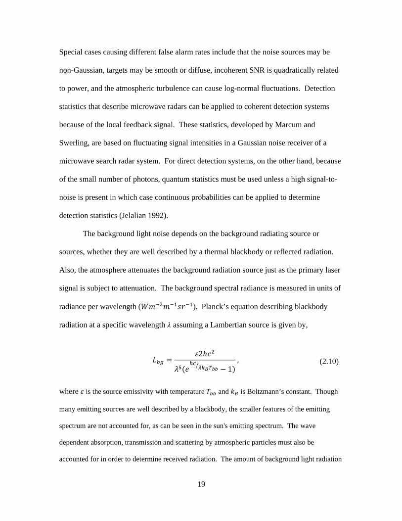
The background light noise depends on the background radiating source or
sources, whether they are well described by a thermal blackbody or reflected radiation.
Also, the atmosphere attenuates the background radiation source just as the primary laser
signal is subject to attenuation. The background spectral radiance is measured in units of
radiance per wavelength ( ). Planck’s equation describing blackbody
radiation at a specific wavelength assuming a Lambertian source is given by,
2
1, (2.10)
where is the source emissivity with temperature and is Boltzmann’s constant. Though
many emitting sources are well described by a blackbody, the smaller features of the emitting
spectrum are not accounted for, as can be seen in the sun's emitting spectrum. The wave
dependent absorption, transmission and scattering by atmospheric particles must also be
accounted for in order to determine received radiation. The amount of background light radiation

20
detected by the LADAR receiver is found by integrating the spectral radiance over the receiver
aperture, , field of view,Ω, filter bandwidth, Δ , and transmission losses, . The background
radiance can be approximated by,
ΩΔ .
(2.11)
This approximation is most accurate for narrowband systems looking at a specific wavelength
(Fujii and Fukuchi 2005).
2.3 Relevant Research
2.3.1 Modeling
In order to fully understand the dynamic nature of atmospheric effects on
electromagnetic propagation, several models have been developed. The uniqueness in
the LEEDR model developed by AFIT/CDE is that it incorporates a correlated,
probabilistic climatological database that creates realistic atmosphere profiles. LEEDR
allows for the creation of vertical profiles of temperature, pressure, water vapor content,
optical turbulence, and atmospheric particulates including hydrometeors. The major
advantage of LEEDR’s probabilistic approach is that vertical profiles are produced for a
specific location and time based on the statistical likelihood of that specific profile
occurring. This type of profile is drastically different than a standard atmosphere profile
where density is assumed to vary with height characterized by a dry adiabatic lapse rate.
The standard atmosphere was created by using averages over time at specific altitudes.
Because the standard atmosphere is made of averages at each layer, the entire profile is
not necessarily a profile that has actually occurred. Using LEEDR, an actual ground
weather condition that has existed is chosen from which a profile is built. The user has
the option of choosing a probabilistic percentage of how dry or damp of an atmosphere

21
from within the distribution of atmospheres at a given location. LEEDR has 573 land
locations of surface data to produce probabilistic profiles (Fiorino et al. 2008).
Probability density function databases used in LEEDR are the Extreme and
Percentile Environmental Reference Tables (ExPERT), Master Database for Optical
Turbulence Research in Support of the Air borne Laser, and the Global Aerosol Data Set
(GADS). Molecular absorption is computed for the top 13 absorbing species using the
HITRAN 2010 database with a molecular absorption continuum code. The Wiscombe
Mie model computes aerosol and hydrometeor scattering and absorption. Climatological
turbulence profiles are produced by correlating relative humidities between data from the
Master Database for Optical Turbulence Research in Support of the Airborne Laser
tailored and the ExPERT data base. The Cn2 profiles used are based upon relative
humidity because optical turbulence and relative humidity have been shown to be largely
interrelated, but the exact reason why they are linked is unclear. Cloud-free line of sight
(CFLOS) probability is obtained from the Air Force Combat Climatology Center ground-
to-space CFLOS tables (Fiorino et al. 2009).
Within LEEDR, the boundary layer temperature, as well as dew point
temperature, is allowed to vary with a constant water vapor mixing ratio. The change in
temperature and dew point temperature is calculated using the equations,
1
1, (2.12)
,
(2.13)

22
where g is the gravitational constant, is the latent heat of vaporization of water, is
the saturation mixture ratio of water, is the specific heat of air at constant pressure, R
is the gas constant, is the moist air gas constant, and is the ratio of the molecular
weight of water over the molecular weight of dry air. Because temperature lapses at a
greater rate than the dew point, saturation often occurs within the boundary layer.
Aerosol sizes are greatly affected by the variation in the relative humidity causing a spike
in laser propagation attenuation as seen in Figure 3. Attenuation increases as aerosol
sizes increase with relative humidity, even though number density remains constant
throughout the boundary layer. This spike is often seen in LIDAR measurements but is
not captured in transmission models using a standard atmosphere (Fiorino et al. 2008).
The Fast Atmospheric Signature Code (FASCODE) model has become the
standard for atmospheric radiation transfer, and the background for band model
approaches to radiation transport. FASCODE is a first principles, line-by-line
atmospheric radiance and transmittance model developed by AFRL (Mazuk and Lynch
Figure 3. Example of increased attenuation at top of boundary layer due to swollen aerosols. Left is output from LEEDR, right is a LIDAR measurement (Fiorino et al. 2008).
V. Matthias, J. Bosenber / Atmospheric Research 63 (2002) 221‐245
Raman lidar intercomparison 351 nm/ 355 nm 98/08/11:21:00 22:20 UT
aerosol extinction (1/m)
altitude (m)
MPI 351 nm, Raman IFT 355 nm, Raman MIM 355 nm, dual angle
23
2001). The code was first developed in 1978 by AFRL, Air Force Geophysics
Laboratory as an improvement from the HIRACC algorithm which was developed for a
uniform atmospheric path with constant temperature, pressure and absorber
concentration. FASCODE uses the HIRACC algorithm but approximates the atmosphere
by a series of layers and incorporating the more realistic Voigt line shape. At high
altitudes, the Doppler, Gaussian line shape dominates while at lower altitudes the
pressure broadened Lorentz shape dominates. The Voigt function used in FASCODE is a
weighted sum of the Doppler function and the Lorentz function. The model uses a series
of atmospheric layers to allow for thermodynamic properties and densities of absorber
molecules to vary. The algorithms within FASCODE were developed with accurate
approximations and techniques to minimize computer time. One such technique was the
larger sampling interval at lower altitudes where line shapes are broader. Absorption is
the only attenuating parameter in the original FASCODE model, neglecting scattering
and turbulence effects. Because absorption is the largest attenuating factor in the rural
clear sky atmosphere, FASCODE gives reasonably good transmission and radiance
approximations in these conditions. Considering the computational limitations at the
time, FASCODE was a monumental advance in atmospheric radiation transfer studies
(Smith et al. 1978).
Since its inception, FASCODE has undergone many upgrades. The latest version
of FASCODE now called FASCODE for the Environment (FASE) incorporates the
Department of Energy’s standard radiative transfer model, Line-by-Line Atmospheric
radiation Code (LBLRTM) along with several other upgrades. The major consideration
in the upgrades in FASE is the increased computational capacity of the modern computer.

24
New cross-sections for heavy molecules, improved solar irradiance model, and
Schumann-Runge bands have been added. Also, the code has been formatted for
improved flexibility, maintainability, and usability (Snell, Moncet et al. 1995). Improved
coding issues including line shape and radiance algorithms for H2O and CO2 continua,
code vectorization and array parameterization have been inserted. The spectral range of a
radiation transfer run was increased from 520 cm-1 to 110 cm-1. The index of refraction
calculation was approximated in the previous FASCODE, now replaced with the exact
formulation of the index of refraction as shown by Kneizys et al. (1983). FASE now
accepts HITAN 96 line parameters and upgraded from using 32 species to 36 species. An
upgrade to cloud and rain parameters was implemented. The clouds now have more
advanced adjustable parameters to more realistically specify cloud characteristics. The
LASER calculations option has an enhanced method of specifying the boundary
emissivity or reflectivity and new coefficients for absorption cross-sections (Snell et al.
1996). The merging of FASCODE and LBLRTM with the above upgrades has resulted
in a flexible radiative transfer model, but needs to undergo comparisons with other
models and validation against data sets (Snell et al. 2000).
2.3.2 Previous Research
Several LADAR simulations have been produced in an attempt to accurately
capture environmental effects. For instance, BAE Systems created a complete 3D
LADAR model that incorporated both atmospheric transmission and scattering. The
rigorous treatment of the laser spatial distribution and backscatter based on a Gaussian
pulse with a random distribution gain variance is unique to this model. The BAE model
intricately accounts for the spatial resolution across the pixels of a receiver array.

25
Performance parameters such as the noise equivalent power, signal-to-noise ratio, and
detection probability of a specified LADAR system can be analyzed as a function of
range, gain, or pixels on target. The model is built to incorporate standard atmospheric
parameters from MODTRAN or FASCODE to produce a single path transmission,
extinction coefficient, and scattering-to-extinction ratio. The Air Force optical radiation
backscatter model, BACKSCAT is then used to determine a backscatter coefficient
(Grasso et al. 2006).
Apart from the strengths of the BAE model listed above, there are several
weaknesses. By using standard atmosphere profiles, real boundary layer effects are being
neglected. Also, because only a single scattering coefficient is being used, the large
scattering difference above and below the boundary layer is being averaged. Noise
sources included in the model are detector dark current, solar reflection off the target,
target blackbody emission, and laser backscatter. The laser backscatter is only taken at
one range location inside the gate. Also, the solar scatter off of atmospheric particles is
neglected. Solar scatter in the receiver field of view many times is the primary noise
source for a LADAR system. Incorporating LEEDR atmosphere profiles into LADAR
models such as that created by BAE or those described by Brown et al. (2005) and
Telgarsky et al. (2004) can allow for a complete characterization of the atmosphere.
Integrating LEEDR’s ability to capture the variability of scattering and extinction
coefficients with altitude, boundary layer effects, and account for solar atmospheric
scatter can make LADAR models more accurate.
An enhanced atmospheric effects model is important to the LADAR community
as recent advances in technology have made available to the LADAR system designer a

26
multitude of options. Several wavebands and their compatible detectors are now
available to choose from. Because of this increase in options it is important to study the
accompanying trade space. In a study by Osche and Young, theoretical comparisons
were made between a 1.54, 2.092, and 10.59 μm wavelength systems. Available laser
systems and their accompanying detectors were compared along with atmospheric effects
at their respective wavelengths. The atmospheric effects were produced with
FASSCODE and MODTRAN using rural, urban, and maritime aerosol models with a
mid-latitude summer standard atmosphere. Fog and rain conditions were also considered.
The study compared range visibility at the different wavelengths with different
environmental conditions. The study concluded that near infrared systems (1.54 and
2.092 μm) do not suffer from water absorption at long ranges like the far infrared systems
(10.59 μm) experience. Far infrared systems outperform near infrared systems being able
to penetrate fog (Osche and Young 1996).
Past research has been done on an assessment of LADAR at 1.0642 µm and 1.557
µm signal-to-noise ratios comparing LEEDR to standard atmosphere profiles. The
standard profiles were MODTRAN with rural aerosols. The assessment actually used
HELEEOS which contains the LEEDR package within it. Variations in the boundary
layer, heavy rain, thick fog, and cloud-free line of sight probabilities were evaluated.
Two geometries were examined with the laser at an altitude of 1525 m with a path length
1530 m and 3000 m to a ground target. The signal received was calculated using the
standard laser radar equation for extended Lambertian targets,
∙4
∙ ∙ ∙ , (2.14)

27
where is the power received, is the power transmitted, is the aperture diameter,
is the slant range, is the optimal reflectance (33.33%), is the roundtrip
transmittance through the atmosphere, is the system optical efficiency, and is the
receiver optical efficiency. The noise was calculated using the noise equivalent power
equation,
∙
2, (2.15)
where is the noise equivalent power, is Planck’s constant, is the speed of light,
is the LADAR wavelength, is the bandwidth, and is the quantum efficiency. These
equations contain many approximations and neglect the background radiation. In the
study, climatologically based transmittance values were significantly less than those
produced with the standard profile over the ocean due to sea salt aerosols being
hydroscopic. Overall, standard profiles gave an overly optimistic estimate of
transmission, and therefore signal-to-noise ratios. For heavy rain conditions, LADAR
systems were shown to be severely limited. The 150 m thick fog layer reduced the
system capability by 93% for the oblique geometry and 75% for the vertical geometry
(Fiorino et al. 2009).
Another study using LEEDR to examine LADAR showed that 1 to 2 µm
wavelengths had little capability in cloud-free heavy rain but still outperformed sub-
millimeter to millimeter radar. LADAR had no performance through clouds or fog, while
radar is only slightly affected in these conditions. However, due to a large number of rain
drops being very nearly the same size as the sub-millimeter to millimeter wavelengths of
the radar, and raindrops being somewhat transparent in the µm wavelengths, LADAR

28
outperforms radar in heavy rain conditions. This study used very similar techniques to
the previous study of LEEDR to standard atmosphere profiles in determining signal-to-
noise ratios (Fiorino et al. 2010).
A major advantage of LADAR is that the laser signal is very narrow making it
covert. The signal is concentrated to a specific region and is not being spread as is
traditional radar. Off-axis scattering from the laser hitting atmospheric particles and
physical objects though can be detected by an observer not collocated with the system. In
a recent study, off-axis laser scatter has been detectable at about a 1 km range and an off-
axis angle of 1.22 degrees for a 1 to 5 watt laser. The range and off-axis detectable angle
are expected to be much greater for a more powerful laser. AFIT’s HELEEOS code was
used to model the off-axis scatter, allowing scatter by molecules and aerosols to be
observed at an off-axis point while incorporating spreading and blooming effects.
Aerosol distributions along the laser and the observer path were accomplished by
determining the visibility and climatological aerosols for southwestern Ohio (Fiorino et
al. 2010). The modeled results were compared to measured data from a turbulence laser
profiler beam that was imaged off-axis with a calibrated camera array. In order to see the
off-axis signal, a background subtraction algorithm was used. Radiance values were
averaged over several frames when the laser was off, and then subtracted from frames in
which the laser was on. Temporal fluctuations caused the noise to remain too high for
the signal to be detected. Because the majority of the frame is background noise, an
additional noise subtraction was done by building a histogram to determine the
background radiance. Subtracting out the rest of this noise sufficiently minimizes the
background allowing the scattered signal to be seen. The background still contained
29
noise which could not be eliminated. The HELEEOS-modeled off-axis irradiance was
within two orders of magnitude of the measured irradiance. Considering the measured
values were on the order of 10-8 W/m2, the modeled values gave a good approximation.
The agreement was not close enough to serve as a validation for HELEEOS (Fiorino et
al. 2010).
Although previous work has been accomplished in using atmospheric models to
characterize the effects the atmosphere may have on LADAR propagation, a first
principals complete integration of the physics included in LEEDR has not. The physics
other models ignore include an increase in scattering at the top of the boundary layer,
climatological variation, and turbulence effects. Although LEEDR has been used
previously to produce worldwide signal-to-noise ratios, only atmospheric transmission
was used in conjunction with an arbitrary sensor noise level. Presented here is the first
study using LEEDR that includes atmospheric transmission and scattering effects on a
LADAR systems performance.
2.4 Summary
By introducing the relevant science and past research in the current literature that
pertains to modeling LADAR propagation through the atmosphere, the reader is now
better prepared to understand the methodology of this work. This thesis combines the
science of atmosphere radiation transfer, laser remote sensing, and advanced physics-
based models. Now that these subject areas have been thoroughly introduced, a detailed
account of the approach taken in using LEEDR to produce simulations of LADAR
signal-to-noise ratios and what steps were taken to accomplish this is shown in Chapter
three.

30
III Methodology
3.1 Chapter Overview
The purpose of this chapter is to give a detailed account of the approach taken to
demonstrate if there are advantages when modeling LADAR propagation using location
specific probabilistic atmospheric characterizations such as those created by LEEDR. An
explanation and overview of the tools used and how they were exploited is discussed.
The modeled scenarios for comparing signal-to-noise are laid out. The process of
creating signal-to-noise values using LEEDR is explained along with how comparisons
were made against standard atmosphere characterizations and assessments done with
FASCODE.
This research contains two main parts, first to compute worldwide signal-to-noise
ratios, and second to produce images at a specified location incorporating signal and
noise returns. All results are for a simulated pulsed direct detect system operating in
Geiger mode. Both parts were accomplished using the tools described here in
combination with Matlab scripts that are included in Appendix A. The global signal-to-
noise ratios are completed for airborne LADAR system geometries targeting objects at
the ground. A low altitude short range engagement along with a high altitude long range
engagement is examined. The low altitude engagement has the platform at 1,530 meters
Above Ground Level (AGL) with a slant path of 3,000 meters. The high altitude
engagement has the platform at 10,000 meters AGL with a slant path of 50,000 meters.
The completely vertical path for both the low and high altitude scenarios is also analyzed.
The low altitude engagement is a possible flight profile for small remotely piloted aircraft
(RPA) while the high altitude engagement is a possible flight profile for a traditional

31
manned aircraft. Both the slanted and vertical geometries are studied here to demonstrate
the effects different paths through the atmosphere have on laser propagation.
Three wavelengths are considered, 1.0642, 1.56, and 2.039 μm. All modeled
runs are completed for clear sky conditions, meaning no clouds or precipitation, and with
the sun directly overhead at a zero zenith angle. The zero zenith angle for the sun is
chosen to keep the geometry simple with platform, target, and sun in the same plane.
LEEDR-produced signal-to-noise ratios are computed for the worldwide 573 ExPERT
sites. The ExPERT atmosphere, also referred throughout this document as the LEEDR
atmosphere, is taken for a summer day at 1500-1800 local when the boundary layer is
fully developed. The 50th humidity percentile is chosen along with Global Aerosol Data
Set (GADS) aerosol profiles for the LEEDR atmosphere. ExPERT site signal-to-noise
ratios are compared to signal-to-noise values produced for various standard atmospheres
and standard aerosol profiles. FASCODE transmissions are computed using Phillips
Laboratory ExPERT User Software (PLEXUS). LADAR target signal returns are created
from these transmissions. Signal-to-noise ratios are then found by using the standard
atmosphere computed noise. Developing noise sources with FASCODE is beyond the
scope of this study. This "FASCODE" signal-to-noise is then compared to LEEDR
created target signal returns. Although this is not a fair assessment of FASCODE as the
signal is only half the equation, it does give insight into the significance of using different
total path transmissions in computing the target signal.
For the purposes of this study, only atmospheric signal and noise values are
considered. All other sources of noise due to the actual LADAR sensor are ignored.
LASER speckle noise is also ignored. Given the intent of this study to compare

32
atmospheric propagation models, the signal and noise returns at the LADAR platform are
computed before entering the actual receiver optics. Signal returns for the down looking
engagements are based on a Lambertian reflecting flat target normal to the LADAR beam
with a 10% reflectivity. Noise returns are comprised of any energy sources that did not
originate from the laser reflecting off the target. The noise sources are laser backscatter
from atmospheric particles, solar reflection off the target, solar scatter off atmospheric
particles in the field of view, and blackbody emission from the target. Signal-to-noise
ratios are then simply computed by dividing the total signal photons by the noise photons.
To produce images incorporating signal and noise returns, images of a 2 m tip to
tail remotely piloted aircraft are created using the High Energy Laser System End to End
Model (HELSEEM). The short and long range slant paths are examined, except this time
the platform is located on the ground looking up. The HELSEEM configuration looking
at the RPA was originally created for the AFIT CDE RPA tracking system. Noise returns
and transmission values are calculated using ExPERT and standard atmosphere profiles
in LEEDR. The noise is incorporated into the pixel values from HELSEEM giving a
visual demonstration of the effect the noise sources have on resolving the target. After all
noise sources are included, the image is then fed through AFIT CDE's light tunneling
algorithm using MZA Corporation's implementation of Light-Tunneling within
WaveTrain. For this research, LEEDR-produced climatological turbulence profiles are
inserted into the algorithm which simulates blurring due to atmospheric turbulence. Once
again only atmospheric effects were considered, ignoring the noise contributions and
effects from the LADAR receiver.

33
3.2 Tools Used
3.2.1 Laser Environmental Effects Definition and Reference (LEEDR)
LEEDR produces worldwide probabilistic profiles based on historical weather
data and predicts radiation transfer through the atmosphere. The primary objectives as
stated in the user's manual are:
1. To create correlated, vertical profiles of meteorological data and environmental effects such as gaseous and particle extinction, optical turbulence, and cloud free line of sight.
2. To allow graphical access to and export of the probabilistic data from the ExPERT database (LEEDR User Guide Version 3.0 2011).
Chosen atmospheric parameters create the desired profile from which absorption,
scattering, and total extinction are calculated. Atmospheric inputs include any global
location, summer or winter season, local time of day in three hour blocks, relative
humidity percentile conditions, a standard atmospheric condition, and a specified aerosol
effects model. If one of the 573 red dot locations is selected, as seen in Figure 4, then
specific site surface and upper air probabilistic data is pulled from the ExPERT database.
The atmosphere tab inputs include eight turbulence profiles, two wind models, and
various rain and cloud types at different altitudes. Among the available turbulence
profiles is a climatological profile, a novel feature of LEEDR. The climatological
turbulences are produced by correlating the temperature and relative humidity percentiles
in the ExPERT database to percentage values in the Master Database for Optical
Turbulence Research in Support of the Airborne Laser (Fiorino et al. 2008). The laser
and geometry tab allows for a desired laser wavelength and geometry.

34
3.2.2 High Energy Laser End-to-End Operational Simulation (HELEEOS)
HELEEOS models dynamic high energy laser weapon engagements predicting
laser atmospheric propagation, radiation at the target, and ultimately a probability of kill
statistic. In the laser engagement, the target and platform can move in any direction in
space with specified directions, velocities, and accelerations (Fiorino et al. 2009).
LEEDR is the atmospheric propagation package used within HELEEOS. For this
research, LEEDR atmospheres were created in HELEEOS. HELEEOS was originally
created for high energy laser weapon engagements, but has some very useful aspects for
LADAR propagation as well. Running HELEEOS was advantageous because of features
such as the ability to save settings and computing a diffraction spot size on the target
based on the user-defined wavelength, exit aperture, and turbulence profile. A 1 cm exit
Figure 4. LEEDR inputs screen

35
aperture and probabilistic turbulence are used throughout this study. The HELEEOS
inputs screen is nearly identical to the one found in LEEDR except for the additional
input tabs to specify the laser optics and dynamic engagement.
3.2.3 Phillips Laboratory ExPERT User Software (PLEXUS)
PLEXUS is a user oriented software package that integrates seven of the Air
Force Research Laboratory atmospheric and astronomical background codes. The
integrated codes are the Department of Defense standard spectral radiance and
transmittance models for the atmosphere. The software provides a graphical user
interface, as seen in Figure 5, which allows the user to make various selections to create
outputs for physically realistic simulations. PLEXUS also contains tools to display and
analyze spectral transmission and radiance outputs (Help for PLEXUS 2006).
The 2006 release of PLEXUS 3.0 beta 1 is used in this study. The 1997 release of
FASCODE 3 with HITRAN 2000 is contained in PLEXUS and is run to compute laser
line transmission. According to the user's manual, FASCODE "is a first principle code
which provides high resolution spectral radiance based on line-by-line calculations. This
code provides the accuracy typically required for laser propagation applications (Help for
PLEXUS 2006)."

36
3.2.4 High Energy Laser System End-to-End Model (HELSEEM)
HELSEEM is a flexible open architecture code that simulates high energy laser
system scenarios. The open architecture is achieved by using the Joint-services Message
Passing Simulation (JMPS) framework from which different components can be easily
added, subtracted or modified. The model was created to be an all purpose simulation
platform for the high energy laser community that caters to various users, fidelity levels,
and scenarios. HELSEEM incorporates high-performance legacy codes and has the
ability to build wrappers around additional code (Ritter et al. 2009).
AFIT CDE is in the process of building a RPA tracking simulation system built
on the HELSEEM architecture which is then fed into atmospheric, light-tunneling, and
sensor effects code. The RPA tracking HELSEEM code produces an illuminated pristine
image of a target from incident laser radiation without atmospheric or blurring effects, as
seen in Figure 6. The pristine image was used in this research, and external noise sources
Figure 5. A few of the PLEXUS input screens and the output screen with a transmission and radiance plot

37
and turbulence effects were added. The code was used in simple laser one-on-one mode
and run through the Windows command prompt. Some of the inputs into the model and
their settings for this research are included in Table 1.
Table 1. HELSEEM input parameters and values used in this study.
Input Name Input Value Obscuration 0.0001 m Beam quality 1.3 Active center of receiver 1.0642 μm, 1.56 μm, and 2.039 μm Active band of receiver 4 nm Laser center 1.0642 μm, 1.56 μm, and 2.039 μm Laser power 20 MW
Camera spacing Varied based on geometry to maintain a 6.144 m field of view
Resolution 512 Full width half max of laser upon exiting 0.01 m Target location (x, y, z coordinates in m) (0, 2580.5, 1530) and (0, 48989.8, 10000) Sun location Zero zenith
Laser focus Varied based on geometry to maintain a 2.9 m full width half max spot size at the target
3.2.5 Light-Tunneling within WaveTrain
Light-Tunneling is a computationally more efficient approach within WaveTrain
than the traditional Incoherent Reflector model that involves spanning the scene with
Figure 6. Image outputs from HELSEEM. From left to right the images are, the beam spread in green and the field of view in yellow at the RPA, the Gaussian beam spot at the target, and last is the return signature of the RPA.
x [m]
y [m
]
-6 -4 -2 0 2 4 6
-5
-4
-3
-2
-1
0
1
2
3
4
50
1
2
3
4
5
6
7
8
9
10
38
many independent speckle realizations. The basic idea of the more efficient approach is
to propagate a number of point sources and interpolate the point spread function, also
known as the blur function, between these points at the receiver. WaveTrain produces
the point spread functions by propagating the point sources through the defined
turbulence profile. Superposition is leveraged in that the resulting intensity at any pixel
is the sum of its own and the overlap of nearby pixel blurring intensities from the
interpolated point spread function. The blurring effects are implemented by creating a
Gaussian centered at each of the pristine image pixels and then shifted by a x and y
translation based upon the point spread function (Beardmore 2006).
For this study, the LEEDR-produced climatological Cn2 profiles are fed into
WaveTrain. An evenly spaced 16 by 16 point grid of point sources is propagated.
Although it is possible to use fewer point sources by concentrating points on the target to
optimize the routine, this is not necessary for the limited number of implementations
performed. Fifteen equally spaced phase screens are used. These phase screens are
determined in WaveTrain and represent the optical aberrations encountered along the
path.
3.3 Signal Calculations
A pulsed LADAR system gates a distance around the target to suppress the
background and laser backscatter. Within this gate are thousands of bins that determine
the depth resolution. In other words, the receiver only opens up after a certain amount of
time after the pulse has left the laser and then registers the signal based on an integration
time. This integration time is also the width of a bin, usually equal to the pulse length in
time. A pulsed Geiger mode LADAR system was used for this analysis. A Geiger mode

39
system uses avalanche photo diodes (APDs) that are very sensitive allowing for a single
photon to be detected. When a photon is detected, the system counts it as a return
"saturating" the system. This makes the system very sensitive, but unable to determine
how many returns were actually detected as only one return in a single bin will be
detected. Also, only one return will be registered per pulse. In reality, the system will be
composed of a two dimensional array of APDs which will allow the system to paint a
picture of the scene. Dark current from within the sensor itself can also set off an APD,
but this is ignored as the study concentrated on only the atmospheric effects. Because
any photon can set off an APD, the background light cannot be subtracted and must be
considered noise.
The signal was created for a single laser pulse with an assumed rectangular
function in time reflecting off a flat Lambertian target. An ideal laser is used in which
only a single wavelength is being transmitted. The returned signal irradiance is then a
function of the surface normal angle, , incident irradiance, , target reflectance,
, laser spot size area, , atmospheric transmission, , target to LADAR platform
range, , and the radiation dispersion solid angle, defined by the equation
cos.
(3.1)
The term is the illuminated area seen by the detector and in some instances may be
limited by the field of view of the detector (Richmond and Cain 2010).
Equation 3.1 gives the target return in irradiance that will only appear in the target
bin. In actuality, the signal could be spread over two bins but for this study, it was
assumed that the signal fits perfectly into one bin. Because any photon can set off the
APD, the noise calculated for this research was the total number of noise photons within
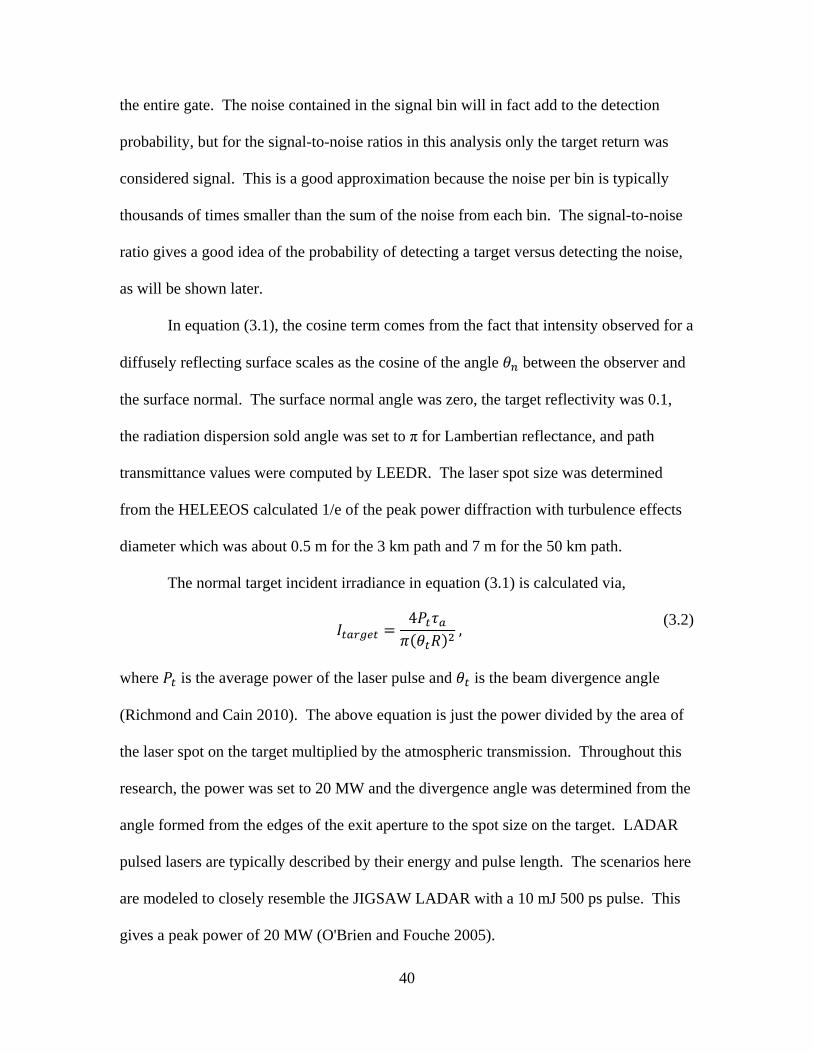
40
the entire gate. The noise contained in the signal bin will in fact add to the detection
probability, but for the signal-to-noise ratios in this analysis only the target return was
considered signal. This is a good approximation because the noise per bin is typically
thousands of times smaller than the sum of the noise from each bin. The signal-to-noise
ratio gives a good idea of the probability of detecting a target versus detecting the noise,
as will be shown later.
In equation (3.1), the cosine term comes from the fact that intensity observed for a
diffusely reflecting surface scales as the cosine of the angle between the observer and
the surface normal. The surface normal angle was zero, the target reflectivity was 0.1,
the radiation dispersion sold angle was set to π for Lambertian reflectance, and path
transmittance values were computed by LEEDR. The laser spot size was determined
from the HELEEOS calculated 1/e of the peak power diffraction with turbulence effects
diameter which was about 0.5 m for the 3 km path and 7 m for the 50 km path.
The normal target incident irradiance in equation (3.1) is calculated via,
4,
(3.2)
where is the average power of the laser pulse and is the beam divergence angle
(Richmond and Cain 2010). The above equation is just the power divided by the area of
the laser spot on the target multiplied by the atmospheric transmission. Throughout this
research, the power was set to 20 MW and the divergence angle was determined from the
angle formed from the edges of the exit aperture to the spot size on the target. LADAR
pulsed lasers are typically described by their energy and pulse length. The scenarios here
are modeled to closely resemble the JIGSAW LADAR with a 10 mJ 500 ps pulse. This
gives a peak power of 20 MW (O'Brien and Fouche 2005).

41
3.4 Noise Calculations
The noise considered in this research is any external sources of energy that do not
originate from the reflection of the laser off the target. Three main noise sources are
examined, laser light that is backscattered off of atmospheric particles, sunlight that is
scattered in the field of view back to the receiver by atmospheric particles, and the
reflection of sun light off the target. Blackbody radiation is also examined, but is
negligible for the wavelengths and target temperatures considered. These sources are
noise as they are always present and contain no distance information.
Depending upon the pulse repetition frequency and the dwell time on a target, a
statistical analysis may be done to subtract out noise returns. This is a result of the target
returns all being concentrated within a single bin while the noise returns will be spread
out over the entire gate. For this study, it is assumed this statistical analysis cannot be
done because either the LADAR operated for a very short amount of time or is scanning
very quickly in which case there is not a substantial amount of time for many target
returns to be registered within a single bin. Therefore, only single pulse analysis is
accomplished for this study.
The signal-to-noise calculations are computed by dividing the signal irradiance by
the sum of the noise irradiance in each bin over the entire gate. The solar noise from
reflection off the target and scatter off of air particles is constant for every bin, including
the target bin. The only noise source that is not constant over the bins is the laser
backscatter, normally with a peak in the first bin. In creating signal-to-noise ratios, the
units can be kept in irradiance even though by definition the signal-to-noise ratio is the
number of signal photons divided by the number of noise photons. To change to photons,

42
both the signal and noise must be multiplied by the integration time and receiver aperture
and divided by the frequency and Planck's constant. These constants all cancel when
determining the signal-to-noise ratio. The only difference is the time t, which for the
signal is only one bin while the noise is the entire gate. The noise irradiance must be
multiplied by the number of bins, assuming the noise is constant across the gate. The
laser backscatter is not the same in every bin, and therefore, the noise irradiance in
every bin must be summed to find the signal-to-noise ratio according to the
equation,
∑
. (3.3)
The solar reflection and solar scatter is the same in each bin and can just be multiplied by
the number of bins b, but the laser backscatter is different in every bin and must be added
individually. Figure 7 displays the irradiance within each bin across the gate for the 10
km altitude vertical path. Ten percent of the path length was gated, so the bin furthest to
the right is at an altitude of 1000 m being near the top of the boundary layer where
aerosols have swelled. The figure has a sudden jump down after it leaves this region as
depicted by bins before about bin number 1700.

43
The signal-to-noise ratios computed have direct correlation to the probability of
detection and false alarm. This correlation was determined by using Poisson statistics for
the single firing APD detector per gate scenario using the equation,
1 , (3.4)
where f is the fraction of bins in front of the target, one for this study, is the total
number of noise photons, is the number of signal photons, and w is /b where b is the
total number of bins. The probability of no primary electron generation is,
, (3.5)
and the probability of false alarm is,
1 . (3.6)
Figure 7. Irradiance values for each bin with the target irradiance at the zero bin represented by an asterisk. The ExPERT Shanghai 10 km slant path simulation, solid blue line and the standard urban atmosphere values, red dashed line values are displayed.
0 1000 2000 3000 4000 5000 6000 700010
-8
10-7
10-6
10-5
10-4
10-3
10-2
Bin Number
Irra
dian
ce (
W/m
2 )
Shanghai ExPERT with GADS for 10km path

44
The probability of no primary electrons comes from equation (1) from O'Brien and
Fouche,
; ,
1!
, exp , , (3.7)
which is the equation for a Poisson process that m events will occur between times t1 and
t2. For m=0, or that no primary electrons are created, the equation reduces to
exp , . Therefore, the probability of one or more primary electrons is
1 exp , , which is the second term in equation (3.8). For the Geiger mode
LADAR, , is the number of photons in a particular bin. Plugging this into,
exp 1 , (3.8)
the probability of no electron detection can be found. The equation predicts the
probability of the detector firing in the jth bin is determined by the sum of all the photons
before and the number of photons in the jth bin. To determine the probability of not
firing at all is substituted for the second term, 1 , where is the
number of signal photons S. The first term becomes which is the total photons
for all the noise bins. This yields equation (3.5), . From these equations,
probability-of-detection and false-alarm curves as a function of the total number of
photons for several different signal-to-noise ratios are produced. The probabilities are a
function of the total number of photons because no matter how strong the signal is, if
there are a significant number of photons before the target bin, the target will never be
seen (O'Brien and Fouche 2005).

45
From Figure 8, the correlation between, the signal-to-noise ratio and the
probability of detection can be seen. Notice how the probability of detection curve never
rises above the probability of false alarm curve for the signal-to-noise ratio of one case.
Taking the maximum probability of detection for varying signal-to-noise curves and the
probability of false alarm at the same total number of photons yields the plot in Figure 9,
which can be used as a metric.
Figure 8. Probability of detection, solid lines, and probability of false alarm, dashed lines as a function of total number of photons for various signal-to-noise ratios.
0 0.5 1 1.5 2 2.5 3 3.5 4 4.5 50
0.1
0.2
0.3
0.4
0.5
0.6
0.7
0.8
Total Number of Photons
Pro
babi
lity
10
7
42
1
Signal to Noise Ratio

46
3.4.1 Laser Scatter Noise
Molecules, aerosols, and hydrometeors in the path of the laser will cause a portion
of the laser energy to be reflected back to the receiver. When a laser in the visible band is
used in a dusty environment, the entire length of the laser beam is seen; while if it is
operated in a vacuum, only the illuminated spot on an object is observed. The beam itself
is visible because of the scattering of laser light off of particles suspended in the air. For
LADAR systems the back scattered laser intensity can become a major source of noise,
especially when there is no knowledge about where the target may be. This scattering of
laser light can be expressed by the equation,
β4
, (3.9)
Figure 9. Peak probability of detection, solid line and probability of false alarm, dashed line, as a function of the signal-to-noise ratio.
0 10 20 30 40 50 60 70 80 90 1000
0.1
0.2
0.3
0.4
0.5
0.6
0.7
0.8
0.9
1
Signal to Noise Ratio
Pro
babi
lity

47
where is the backscattered laser irradiance, is the path transmittance, is the
phase function, β is the volume scattering coefficient, is the incident irradiance,
is the range to the parcel of air, and is the differential volume element of the laser
(Fiorino et al. 2010). The laser scattering equation was performed for both aerosol and
molecular scattering.
The scattering integral gives the total backscatter for a continuous laser at an
instant in time, but for a pulsed LADAR, the equation represents the total backscatter
noise integrated over the entire gate. The equation is turned into a summation of equally
spaced bins or segments equal to the pulse length of the laser over the length of the gate.
The gate only extended in front of the target bin as there is no laser backscatter beyond
the target. The volumes of the segments are determined from creating cylinders with
diameters found at the center of each segment. The diameters are calculated by linearly
interpolating between the start of the gate diameter and the spot size at the target. The
diameter at the start of the gate is found by determining a beam divergence angle from
the edge of the exit aperture to the spot size at the target. This assumes the entire beam is
in the field of view. Inadvertently, the spot size being calculated using diffraction in
HELEEOS was slightly larger than the chosen field of view for the 2.039 μm wavelength.
A slight error in the 2.039 μm wavelength signal-to-noise results when laser backscatter
is dominate, thought to be less than 10% to high, is introduced. The phase function and
volume scattering coefficients are linearly interpolated from the calculated LEEDR
values. LEEDR produces 1,000 equally spaced atmospheric layers with these
coefficients for any given engagement geometry. The phase function defines the amount
of scattered energy per solid angle in a particular direction. The phase function is

48
dependent upon the direction of energy scattering from its original direction represented
by the angle θ as well as altitude, while the volume scattering coefficient is only
dependent on altitude. Examples of the phase function plotted against scattering angle
and the scattering volume coefficients plotted against altitude are shown in Figure 10.
The plots in Figure 10 are created for a 1.0642 μm laser from the Jan Mayen ExPERT
50th humidity percentile atmosphere with GADS aerosols for a summer day between
1500 and 1800.
The incident irradiance in equation (3.9) is found by multiplying the laser
power by the transmission to the center of each volume element and dividing by the beam
Figure 10. From left to right, top to bottom, molecular phase function, aerosol phase function, molecular volume scattering coefficient, and the aerosol volume scattering coefficient.
0 20 40 60 80 100 120 140 160 1800.6
0.7
0.8
0.9
1
1.1
1.2
1.3
1.4
1.5
1.6
(deg)
P(
)
0 20 40 60 80 100 120 140 160 180
10-1
100
101
102
103
(deg)
P(
)
6.8 7 7.2 7.4 7.6 7.8 8 8.2 8.4
x 10-4
0
200
400
600
800
1000
1200
1400
1600
Alti
tude
(m
)
Molecular Volume Scattering Coefficient s
0 0.05 0.1 0.15 0.2 0.25 0.3 0.350
200
400
600
800
1000
1200
1400
1600
Alti
tude
(m
)
Aerosol Volume Scattering Coefficient s

49
cross sectional area. In reality, the cross sectional irradiance in the beam will vary, often
modeled as a Gaussian. For this research, the beam did not need to be resolved as only
the total reflected irradiance was needed. The transmission to each segment center was
found using the equation,
, (3.10)
where is the extinction coefficient at a specified distance , and is the
differential length element. Once again, the extinction coefficients were interpolated
from the LEEDR-produced coefficients. A transmission from the platform to the gate
front was determined and then multiplied by the transmission from the gate front to each
of the segment centers. Multiplying these two transmissions together gave the
transmission from the platform to each segment center in the gate.
Because of the term in the denominator of equation (3.9), the size of the gate
has a large effect on the backscattered irradiance, especially if the gate is allowed to
extend the entire distance from the target. The plot in Figure 11 demonstrates the effect
the gate size has on the backscattered irradiance. It is created with an ExPERT site
atmosphere for a summer day between 1500-1800 local at Bucharest, Romania. The
platform is at an altitude of 1530 m with a 3 km slant path and a laser power of 100 W.
The exit aperture is 1 cm with a spot size at the target of 40 cm.

50
3.4.2 Solar Scatter Noise
It should be noted that only the single scatter is considered in this scenario and is
a good approximation for clear sky conditions. On the other hand, inside clouds,
radiation can scatter thousands of times within a very short distance. Equation (3.9) is
used in computing the solar scatter noise. The phase function and volume scattering
coefficient are once again interpolated from LEEDR but this time for the entire range
from the platform to the target. The range was segmented into 100 equally spaced
volume elements with a square cross sectional area at the segment centers determined by
the length of the side of the square detector and the receiver optics focal length. The
volume elements for the solar scatter are in fact the field of view volume modeled as a
pyramid broken into segments starting as a point at the platform and extending to a
square field of view area at the target. The incident irradiance is calculated by taking the
Figure 11. The back scattered laser irradiance as a function of the fraction of the beam gated in front of the target.
0 0.1 0.2 0.3 0.4 0.5 0.6 0.7 0.8 0.9 110
-10
10-9
10-8
10-7
10-6
10-5
10-4
Fraction of Beam Gated
Bac
k S
catt
ered
Irr
adia
nce
(W/m
2 )

51
solar spectrum at the top of the atmosphere, integrating over the receiver bandwidth, and
then multiplying by the path transmittance through the atmosphere to the segment
centers. The 2 nm resolution American Society for Testing and Materials (ASTM) 2000
extraterrestrial solar spectra is used for the solar spectral irradiance at the top of the
atmosphere and is shown in Figure 12. Note that at 1 μm, the solar irradiance is six times
larger than that at 2 μm. With this information, the noise in our system from the sun is
expected to be much less for the 2.039 μm as compared to the 1.0642 μm wavelength.
The following equation is used to find the incident solar irradiance,
, (3.5)
where is the detector bandwidth and is the top of the atmosphere solar spectral
irradiance. The ASTM solar spectrum is numerically integrated over the receiver
bandwidth from ten equally spaced interpolated points within the bandwidth. After the
Figure 12. Spectral irradiance at the top of the atmosphere (ASTM 2000)
0 0.2 0.4 0.6 0.8 1 1.2 1.4 1.6 1.8 20
200
400
600
800
1000
1200
1400
1600
1800
2000
2200
Wavelength (m)
Spe
ctra
l Irr
adia
nce
(Wm
- 2 m
- 1)

52
solar spectrum over the bandwidth is determined, it is then multiplied by the atmospheric
transmission , which changes with the path length the radiation must travel through the
atmosphere. Equation (3.4) is used to compute the transmission from the top of the
atmosphere to the segment centers and the transmission from the segment centers to the
receiver. The solar incident path lengths through the atmosphere are calculated from the
sun's zenith angle using trigonometry from the center of the earth. One thousand
atmospheric layers are created in the solar incident radiation calculation, interpolating the
extinction coefficients from the LEEDR calculated extinction coefficients. Unlike the
laser, the sun's irradiance does not change or spread because of the increase in the size of
the volume element. In a vacuum, the sun equally illuminates the top and bottom of the
atmosphere, mainly due to the sun's great distance from Earth.
3.4.3 Solar Reflection Noise
The solar reflection off the target is calculated the same way the signal is
determined using equation (3.1). Looking at equation (3.1), the surface normal equation
is now dependent upon the location of the sun (zero zenith for this study), dA is now the
entire field of view, and the incident irradiance is now the incident solar radiation. The
target reflectance is kept at 10%. The equation assumes that the target surface fills the
entire field of view of the detector.
To find the incident solar irradiance, the solar spectral irradiance at the top of the
atmosphere was integrated over the receiver bandwidth and multiplied by the LEEDR
computed transmission through the atmosphere. Once again, the ASTM 2000
extraterrestrial solar spectra are used along with equation (3.5). The path length is
ultimately determined from the solar zenith angle. The sun zenith angle has very little

53
effect on the transmission when the sun is overhead but as the sun drops further in the
sky, the transmission begins to change more rapidly (see Figure 13). This is akin to
taking a tape measure a few inches from perpendicular to the ceiling. Changing the angle
of the tape measure increases the distance the tape measure must extend to touch the
ceiling, with the greatest increases occurring at the higher angles.
3.4.4 Blackbody Noise
Any object that is not at absolute zero (K) radiates energy. This energy is the
blackbody radiation and is determined by the equation,
2
1,
(3.6)
Figure 13. Solar transmittance as a function of sun zenith angle for the summer 1500-1800 50th humidity percentile LEEDR ExPERT atmosphere at Bucharest, Romania
0 10 20 30 40 50 60 70 80 900
0.1
0.2
0.3
0.4
0.5
0.6
0.7
0.8
0.9
1
Sun Zenith Angle
Tra
nsm
ittan
ce

54
where is the linear field of view (m), is Planck's constant (6.626 x 10⁻³⁴ J s), is
the speed of light (2.998 x 10⁸ m/s), is Boltzmann's constant (1.381 x 10⁻²³ J/K), and
is the objects temperature (K) (Petty 2006).
The temperature of the target for this analysis was assumed to be 300 K or about
80° F. For imperfect blackbody objects, the blackbody radiation is then multiplied by an
emissivity. For this study, the blackbody radiation without an emissivity proved to be
negligible because of the shorter wavelengths, narrow band, and low temperature. Figure
14 shows that blackbody emission nearly goes to zero for wavelengths shorter than 2.5
μm.
3.5 HELSEEM Images
HELSEEM returns pristine images in the form of a matrix containing irradiance
values for each pixel. The images are referred to as pristine as they contain no
Figure 14. Black body curves for temperatures between 200 and 300 K (Petty 2006).

55
atmospheric extinction or turbulence effects. In generating images to display
atmospheric noise effects, the pristine image is used as the signal. The previously
described methods are employed to compute noise. The HELSEEM code used is for an
up-looking geometry, so the Matlab scripts for the down-looking signal and noise
calculations were modified to be compatible for an up-looking engagement. A 3 km slant
path with a target at 1530 m and a 50 km slant path with a target at 10 km at the
Shanghai, China is examined. Atmospheric effects based on the ExPERT atmosphere
with GADS aerosols are compared against the mid-latitude north standard atmosphere
with MODTRAN urban aerosols. A comparison against using FASCODE transmissions
for the signal propagation as well as a comparison against the ExPERT atmosphere with
MODTRAN aerosols is executed.
One of the major differences between the down-looking geometries done
previously for the global plots and the up-looking engagements here is that the solar
scatter is no longer only the scattered sunlight in the field of view in front of the target,
but also beyond the target. In order to incorporate the noise onto the signal matrix, both
the signal and the noise are converted to radiance values in watts per meter squared per
steradian. The image radiance values are found by dividing each pixel irradiance value in
the image by its steradian value found by dividing the pixel area on the target by the
squared range to the target. The computed noise irradiance is for the entire field of view
so it is converted to radiance by dividing the field of view area by the squared range to
the target. The solar reflection is computed in HELSEEM by doing a separate run in
which the laser is off and only the sun's illumination creates the image.
56
Once the image and the noise are both in radiance units, each noise component is
added. It is assumed that if the noise is greater than or equal to the signal, the signal is no
longer visible. After the solar reflection is incorporated, the signal with the subtracted
solar reflection is multiplied by the total path transmittance. The solar scatter behind the
target is only added to all the zero signal image pixels because the RPA blocks all of the
radiation directly behind it. The remaining noise is incorporated by adding the noise to
every pixel with a value less than the previously added noise plus the current noise up to
the total noise value. This process is illustrated in Figure 15. Imagine filling up a
bathtub with an object in the middle; parts of the object slowly are submerged as the
water level rises. When outputting the image, each pixel was divided by the noise
resulting in units of signal-to-noise. This method assumes that no signal under a signal-
to-noise ratio of one will be visible.
After all noise effects are accounted for, the image matrix of radiance values is
fed into the Light-Tunneling within WaveTrain algorithm. LEEDR climatological winds
and climatological turbulence profiles are used in the algorithm. The final image has
atmospheric transmission, noise, and turbulence effects included.

57
3.6 Summary
The method described here to show if LEEDR ExPERT atmospheres with GADS
aerosols are advantageous to use in simulating LADAR over a standard atmosphere with
a standard aerosol profile has two main parts. The two main parts are to produce signal-
to-noise ratios for a Lambertian target, and then generate images to show signal-to-noise
effects. Only atmospheric noise effects are considered in this study. Both parts are
accomplished for ExPERT atmospheres with GADS aerosols and standard atmospheres
with standard aerosols. By comparing the outputs from the two different atmospheres,
the advantages of using ExPERT atmospheres with GADS aerosols are evident and will
be shown in the next chapter.
Figure 15. Progression of adding noise from left to right, top to bottom, the sun reflection, pristine image, background and transmission, solar scatter, laser backscatter, and finally the turbulence is added.
1.0642m 3km Sun Reflectance (W/(m2sr))
100 200 300 400 500
50
100
150
200
250
300
350
400
450
5000
10
20
30
40
50
60
70
80
90
1001.0642m 3km Pristine Image (W/(m2sr))]
100 200 300 400 500
50
100
150
200
250
300
350
400
450
5000
1
2
3
4
5
6
7x 10
4
1.0642m 3km Atmospheric Transmission with Background (SNR)
100 200 300 400 500
50
100
150
200
250
300
350
400
450
500 1
2
5
10
20
50
100
200
500
1000
1.0642m 3km Transmission and Solar Scattering (SNR)
100 200 300 400 500
50
100
150
200
250
300
350
400
450
500 1
2
5
10
20
50
100
200
500
1000
1.0642m 3km Transmission, Solar and Back Scattering (SNR)
100 200 300 400 500
50
100
150
200
250
300
350
400
450
500 1
2
5
10
20
50
100
200
500
1000ClimoTurb Shanghai 1.0642 m 3km (SNR)
100 200 300 400 500
50
100
150
200
250
300
350
400
450
500 1
2
5
10
20
50
100
200
500
1000
58
IV Analysis and Results
4.1 Chapter Overview
Global signal-to-noise ratios computed using LEEDR atmospheres are presented
here as well as comparisons to standard profiles with standard aerosol distributions, and
FASCODE transmissions. Images of an RPA displaying signal-to-noise is also shown
displaying the difference between LADAR signal-to-noise for an ExPERT site as
compared to a standard atmosphere profile. The reasons for the differences are discussed
as well as the advantages that the probabilistic atmosphere approach brings to the
LADAR modeling problem.
4.2 Results
4.2.1 World Wide Lambertian Target Signal-to-Noise Results
Figure 16 displays the resulting signal-to-noise ratios for the short range 3 km
slant and vertical engagements from an altitude of 1530 m. The left global plots are for
the slant path while the right global plots are for the vertical path. The scale was kept
constant for all wavelengths for each geometry, making it easier to distinguish changes in
the signal-to-noise ratios between different wavelengths. It was necessary to change the
scale between geometries as the signal-to-noise ratios changed drastically. Because the
scale was constant with a linear scale, many locations saturated the scale. This was
necessary in order to keep the scale constant while seeing variations at the 1.0642 μm
wavelength. The majority of contrast can be seen between the 1.0642 μm and 1.56 μm
wavelengths for both geometries. In the 3km slant path geometry plots, several sites with
signal-to-noise ratios hovering around 100 at the 1.0642 μm wavelength jump to over 500

59
at the 1.56 μm wavelength. Looking at the difference between the short range slant and
vertical geometries at the 1.0642 μm wavelength, the signal-to-noise ratios are doubled
for many locations while other locations remain almost the same. The major difference
between locations is the aerosol profiles, and hence the signal-to-noise remains low
regardless of the wavelength at locations with denser aerosols.
Figure 17 displays the resulting signal-to-noise ratios for the long range 50 km
slant and vertical engagements from an altitude of 10 km. The left global plots are for the
slant path while the right global plots are for the vertical path. Again, the scale was kept
Figure 16. Short range slant path and vertical path signal-to-noise ratios for LEEDR ExPERT site atmospheres with GADS aerosols. The platform is at 1530 m altitude looking down at a target on the ground.
0
100
200
300
400
500
0
200
400
600
800
1000
1200
180 W 135 W 90 W 45 W 0 45 E 90 E 135 E 180
90 S
45 S
0
45 N
1.0642 m 3km slant path
90 N
180 W 135 W 90 W 45 W 0 45 E 90 E 135 E 180
90 S
45 S
0
45 N
1.0642 m 1530m vertical path
90 N
180 W 135 W 90 W 45 W 0 45 E 90 E 135 E 180
90 S
45 S
0
45 N
1.56 m 3km slant path 90 N
180 W 135 W 90 W 45 W 0 45 E 90 E 135 E 180
90 S
45 S
0
45 N
2.039 m 3km slant path 90 N
180 W 135 W 90 W 45 W 0 45 E 90 E 135 E 180
90 S
45 S
0
45 N
2.039 m 1530m vertical path
90 N
180 W 135 W 90 W 45 W 0 45 E 90 E 135 E 180
90 S
45 S
0
45 N
1.56 m 1530m vertical path
90 N

60
constant for all wavelengths for each geometry. Notice that the scales are now 0 to 10 for
the 50 km slant path and 0 to 100 for the vertical path. This is more than an order of
magnitude smaller than the short range scale. Once again, the majority of contrast can be
seen between the 1.0642 μm and 1.56 μm wave lengths for both geometries. Also, there
are many regions of the world that remain to have a low signal-to-noise ratio regardless
of the wavelength. These areas are desert and maritime locations. Maritime locations
generally have larger wind speeds increasing aerosols in the air. Sea salt aerosols at these
locations are also hygroscopic being allowed to swell in size with relative humidity.
Desert locations also generally have higher wind speeds causing desert aerosols to
become suspended in the air. Although these particles are not hygroscopic, they are
generally smaller and denser than other regional aerosols.

61
While the global signal-to-noise ratio plots give great insight into atmospheric
climatological conditions and locations that are ideal for LADAR usage, the purpose of
this research is to identify advantages of using ExPERT atmospheres with GADS
aerosols over standard atmosphere profiles with standard aerosol distributions. In order
to accomplish this, the next charts are created to compare standard atmosphere and
aerosol profile types with ten chosen ExPERT sites with the specified type of climate.
The four standard atmospheres and their aerosol types chosen to study are the mid-
latitude north with MODTRAN urban aerosols, mid-latitude north with MODTRAN rural
Figure 17. Long range slant path and vertical path signal-to-noise ratios for LEEDR ExPERT site atmospheres with GADS aerosols. The platform is at 10 km altitude looking down at a target on the ground.
1.0642 m 50km slant path
180 W 135 W 90 W 45 W 0 45 E 90 E 135 E 180
90 S
45 S
0
45 N
90 N 1.0642 m 10km vertical path
180 W 135 W 90 W 45 W 0 45 E 90 E 135 E 180
90 S
45 S
0
45 N
90 N
1.56 m 50km slant path
180 W 135 W 90 W 45 W 0 45 E 90 E 135 E 180
90 S
45 S
0
45 N
90 N 1.56 m 10km vertical path
180 W 135 W 90 W 45 W 0 45 E 90 E 135 E 180
90 S
45 S
0
45 N
90 N
2.039 m 50km slant path
180 W 135 W 90 W 45 W 0 45 E 90 E 135 E 180
90 S
45 S
0
45 N
90 N 2.039 m 10km vertical path
180 W 135 W 90 W 45 W 0 45 E 90 E 135 E 180
90 S
45 S
0
45 N
90 N
E
0
2
4
6
8
10
E
0
20
40
60
80
100

62
aerosols, desert with desert aerosols, and tropical with maritime tropical aerosols. Besides
the specified standard atmosphere and standard aerosol profile signal-to-noise ratios,
FASCODE values incorporating FASCODE transmissions are also included.
Table 2 gives insight into how FACODE transmissions change for different
aerosol types. The transmissions are created by using PLEXUS, which has a graphical
user interface to run FASCODE. In this study, the normal high visibility transmissions
are used except for the urban climate analysis in which case the normal low visibility
FASCODE transmissions are used. The urban low visibility transmissions are originally
thought to have values closer to the those found at urban ExPERT sites with GADS
aerosols.
Table 2. FASCODE transmissions for the different geometries, wavelengths and various aerosol types
Short Range Slant Short Range Vertical Long Range Slant Long Range Vertical (1.53km Alt 3km Range) (1.53km Alt 1.53km Range) (10km Alt 50km Range) (10km Alt 10km Range)
Aerosols 1.0642 μm
1.56 μm
2.039 μm
1.0642 μm
1.56 μm
2.039 μm
1.0642 μm
1.56 μm 2.039 μm
1.0642 μm
1.56 μm
2.039 μm
Normal High
Visibility (23Km)
Urban 0.8511 0.9009 0.8613 0.9211 0.9481 0.9255 0.489 0.6437 0.5155 0.8657 0.915 0.8613
Rural 0.8637 0.9163 0.8779 0.928 0.9564 0.9346 0.5149 0.6835 0.5513 0.8748 0.9261 0.8731
Desert 0.8817 0.9368 0.8915 0.9378 0.9672 0.9419 0.5519 0.7367 0.5804 0.8871 0.9402 0.8822
Maritime 0.7553 0.7879 0.7625 0.8667 0.8855 0.8698 0.3259 0.4075 0.3408 0.7974 0.8343 0.7921
Normal Low
Visibility (5Km)
Urban 0.3771 0.5426 0.5977 0.6083 0.732 0.7679 6.76E‐02 0.1812 0.2093 0.5728 0.707 0.7171
Rural 0.4127 0.6022 0.672 0.6369 0.772 0.8152 8.43E‐02 0.2384 0.2854 0.6014 0.7482 0.7642
Desert 0.4682 0.6896 0.7383 0.6792 0.8273 0.8553 0.1154 0.3404 0.3654 0.6433 0.8045 0.8035
Maritime 0.1812 0.2385 0.2831 0.4187 0.4813 0.5247 1.59E‐02 2.64E‐02 3.43E‐02 0.3874 0.4553 0.4807
The FASCODE atmosphere type in the following charts is created by using the
standard atmosphere and aerosol types for the noise calculations and then using the
FASCODE transmissions for the signal calculations. Although this is not a fair
assessment of FASCODE, it does give insight into the effects using different total path
transmission values has on LADAR performance. The charts also contain the mean
absolute difference and the mean absolute percent difference for both the standard
atmosphere and FASCODE values. Although using the absolute difference does not give
63
any indication of systematic error greater or smaller than the ExPERT site values, it does
give an indication to the variability of the values. This method of analysis is chosen as it
is expected that the ExPERT values will vary greater and smaller than the standard
atmosphere characterization, but how great this variability is shows the importance of
using a probabilistic approach. The percent difference column is actually the ratio of the
absolute mean difference divided by the standard atmosphere or FASCODE value.
Transmissions were also included in the chart to analyze the degree of correlation
between signal-to-noise ratio and transmission values.
From Table 3, urban ExPERT sites with GADS aerosols are relatively well
described by the shorter 1.0642 μm wavelength standard profile having a mean absolute
difference of about 25% for both the short range slant path and the vertical path but is
relatively poor in describing the longer wavelengths. As expected, there does not seem to
be a trend of higher or lower ExPERT values as compared to the standard atmosphere.
The sites seem to be both evenly spread with greater and lower values, with greater
variation at the two higher wavelengths. Analyzing the correlation between the
transmissions and the signal-to-noise ratios shows there is no correlation when the
ExPERT sites are compared to the standard atmosphere values at a specified wavelength.
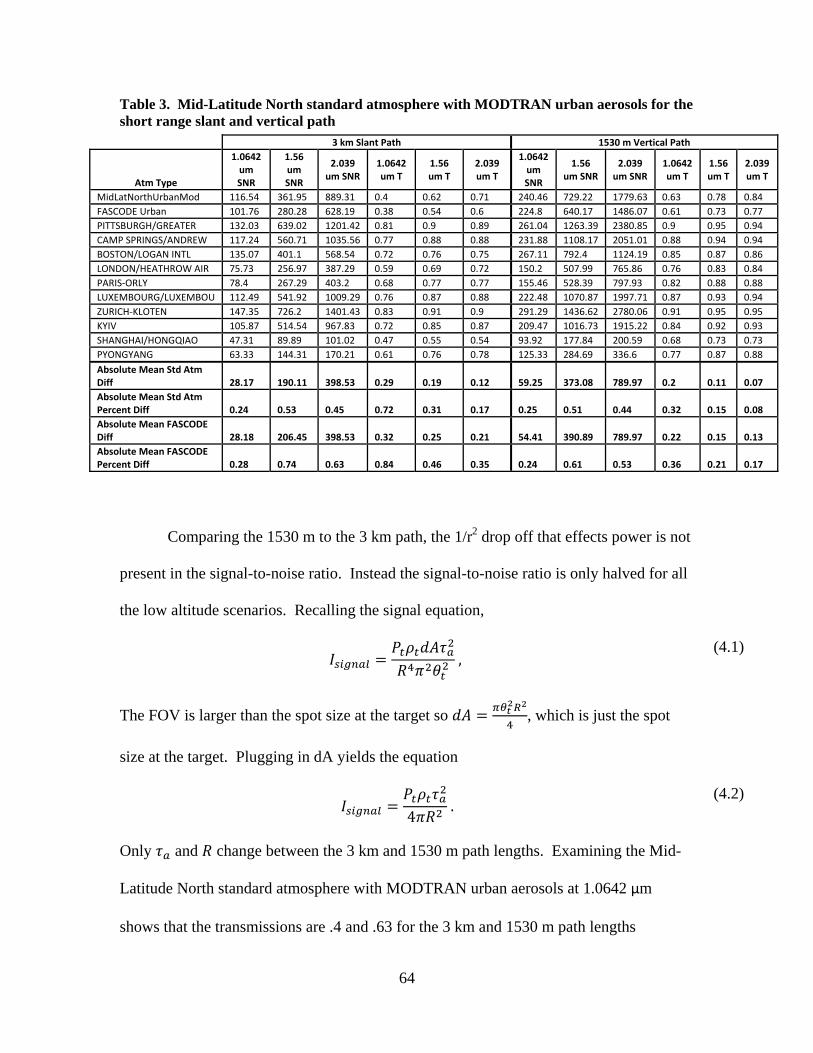
64
Table 3. Mid-Latitude North standard atmosphere with MODTRAN urban aerosols for the short range slant and vertical path
3 km Slant Path 1530 m Vertical Path
Atm Type
1.0642 um SNR
1.56 um SNR
2.039 um SNR
1.0642 um T
1.56 um T
2.039 um T
1.0642um SNR
1.56 um SNR
2.039 um SNR
1.0642 um T
1.56 um T
2.039 um T
MidLatNorthUrbanMod 116.54 361.95 889.31 0.4 0.62 0.71 240.46 729.22 1779.63 0.63 0.78 0.84
FASCODE Urban 101.76 280.28 628.19 0.38 0.54 0.6 224.8 640.17 1486.07 0.61 0.73 0.77
PITTSBURGH/GREATER 132.03 639.02 1201.42 0.81 0.9 0.89 261.04 1263.39 2380.85 0.9 0.95 0.94
CAMP SPRINGS/ANDREW 117.24 560.71 1035.56 0.77 0.88 0.88 231.88 1108.17 2051.01 0.88 0.94 0.94
BOSTON/LOGAN INTL 135.07 401.1 568.54 0.72 0.76 0.75 267.11 792.4 1124.19 0.85 0.87 0.86
LONDON/HEATHROW AIR 75.73 256.97 387.29 0.59 0.69 0.72 150.2 507.99 765.86 0.76 0.83 0.84
PARIS‐ORLY 78.4 267.29 403.2 0.68 0.77 0.77 155.46 528.39 797.93 0.82 0.88 0.88
LUXEMBOURG/LUXEMBOU 112.49 541.92 1009.29 0.76 0.87 0.88 222.48 1070.87 1997.71 0.87 0.93 0.94
ZURICH‐KLOTEN 147.35 726.2 1401.43 0.83 0.91 0.9 291.29 1436.62 2780.06 0.91 0.95 0.95
KYIV 105.87 514.54 967.83 0.72 0.85 0.87 209.47 1016.73 1915.22 0.84 0.92 0.93
SHANGHAI/HONGQIAO 47.31 89.89 101.02 0.47 0.55 0.54 93.92 177.84 200.59 0.68 0.73 0.73
PYONGYANG 63.33 144.31 170.21 0.61 0.76 0.78 125.33 284.69 336.6 0.77 0.87 0.88
Absolute Mean Std Atm Diff 28.17 190.11 398.53 0.29 0.19 0.12 59.25 373.08 789.97 0.2 0.11 0.07
Absolute Mean Std Atm Percent Diff 0.24 0.53 0.45 0.72 0.31 0.17 0.25 0.51 0.44 0.32 0.15 0.08
Absolute Mean FASCODE Diff 28.18 206.45 398.53 0.32 0.25 0.21 54.41 390.89 789.97 0.22 0.15 0.13
Absolute Mean FASCODE Percent Diff 0.28 0.74 0.63 0.84 0.46 0.35 0.24 0.61 0.53 0.36 0.21 0.17
Comparing the 1530 m to the 3 km path, the 1/r2 drop off that effects power is not
present in the signal-to-noise ratio. Instead the signal-to-noise ratio is only halved for all
the low altitude scenarios. Recalling the signal equation,
,
(4.1)
The FOV is larger than the spot size at the target so , which is just the spot
size at the target. Plugging in dA yields the equation
4.
(4.2)
Only and change between the 3 km and 1530 m path lengths. Examining the Mid-
Latitude North standard atmosphere with MODTRAN urban aerosols at 1.0642 μm
shows that the transmissions are .4 and .63 for the 3 km and 1530 m path lengths

65
respectfully. Dividing the 3 km path variables designated by subscript one by the 1530 m
variables designated as subscript two,
,
(4.3)
yields a factor of about 9.5 increase in signal. This is shown by the signal in at the 3 km
path of 0.0115 (W/m2) and the signal at the 1530 m path of 0.1075 (W/m2) making the
actual factor about 9.4. The factor did not come out exactly as the transmission values
were rounded. The same factor is found for the noise if laser backscatter is dominate
which is calculated from
β4
, (4.4)
where and ∗ which yields the equation
β4
, (4.5)
where is the differential path length element. Once again the variables that change
from the 3 km to the 1530 m path are and which yields the same factor of about a
9.5 increase. This means the signal and laser scatter noise are exactly cancelling and the
main difference is the number of bins. The number of bins is decreased by about half
going from the 3 km range to the 1530 m range causing the noise to increase by about
4.25 instead. This is shown by the noise values in at the 3 km path of . ∗
(W/m2) and the noise at the 1530 m path of 4. ∗ (W/m2). The value is not exact
as there are other noise contributions and the numbers were rounded in this
demonstration. The above analysis also shows that once laser scatter becomes the
dominate noise source and if the number of gate bins is kept constant, the signal-to-noise
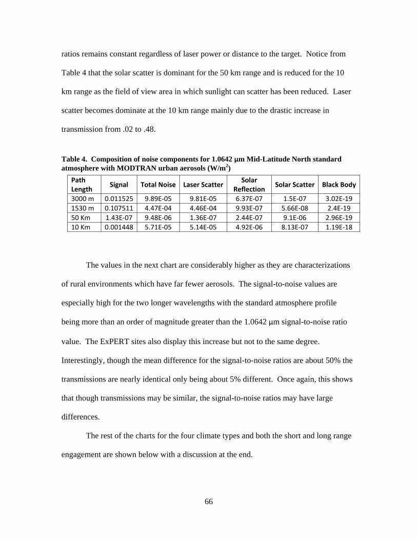
66
ratios remains constant regardless of laser power or distance to the target. Notice from
Table 4 that the solar scatter is dominant for the 50 km range and is reduced for the 10
km range as the field of view area in which sunlight can scatter has been reduced. Laser
scatter becomes dominate at the 10 km range mainly due to the drastic increase in
transmission from .02 to .48.
Table 4. Composition of noise components for 1.0642 μm Mid-Latitude North standard atmosphere with MODTRAN urban aerosols (W/m2)
Path Length
Signal Total Noise Laser ScatterSolar
ReflectionSolar Scatter Black Body
3000 m 0.011525 9.89E‐05 9.81E‐05 6.37E‐07 1.5E‐07 3.02E‐19
1530 m 0.107511 4.47E‐04 4.46E‐04 9.93E‐07 5.66E‐08 2.4E‐19
50 Km 1.43E‐07 9.48E‐06 1.36E‐07 2.44E‐07 9.1E‐06 2.96E‐19
10 Km 0.001448 5.71E‐05 5.14E‐05 4.92E‐06 8.13E‐07 1.19E‐18
The values in the next chart are considerably higher as they are characterizations
of rural environments which have far fewer aerosols. The signal-to-noise values are
especially high for the two longer wavelengths with the standard atmosphere profile
being more than an order of magnitude greater than the 1.0642 μm signal-to-noise ratio
value. The ExPERT sites also display this increase but not to the same degree.
Interestingly, though the mean difference for the signal-to-noise ratios are about 50% the
transmissions are nearly identical only being about 5% different. Once again, this shows
that though transmissions may be similar, the signal-to-noise ratios may have large
differences.
The rest of the charts for the four climate types and both the short and long range
engagement are shown below with a discussion at the end.

67
Table 5. Mid-Latitude North standard atmosphere with MODTRAN rural aerosols for the short range slant and vertical path
3 km Slant Path 1530 m Vertical Path
Atm Type
1.0642 um SNR
1.56 um SNR
2.039 um SNR
1.0642 um T
1.56 um T
2.039 um T
1.0642 um SNR
1.56 um SNR
2.039 um SNR
1.0642 um T
1.56 um T
2.039 um T
MidLatNorthRuralMod 142.94 1689.24 1931.11 0.87 0.95 0.93 283.06 3372.36 3837.15 0.93 0.97 0.96
FASCODE 139.83 1582.07 1727.96 0.86 0.92 0.88 279.95 3260.94 3616.3 0.93 0.96 0.93
MEDFORD‐JACKSON COU 273.5 585.77 690.67 0.92 0.94 0.92 541.56 1157.49 1364.42 0.96 0.97 0.96
WATERLOO MUNICIPAL 114.55 533.73 957.24 0.74 0.86 0.86 226.55 1054.72 1895.33 0.85 0.92 0.93
GRIFFISS AFB/ROME 165.39 712.26 1186.83 0.86 0.93 0.9 326.89 1408.74 2351.79 0.93 0.96 0.95
GRAFENWOEHR 134.26 626.97 1130.09 0.81 0.9 0.89 265.44 1239.5 2238.95 0.9 0.95 0.94
NJANDOMA 174.44 738.74 1218.58 0.82 0.9 0.9 344.78 1461.25 2412.42 0.9 0.95 0.95
TUGULYM 154.79 676.19 1143.7 0.82 0.91 0.9 305.94 1336.97 2264.13 0.91 0.95 0.95
NIZHNEUDINSK 275.68 1129.41 1841.05 0.89 0.94 0.93 545.34 2240.58 3654.47 0.94 0.97 0.96
ZEJA 312.79 1406.03 2554.53 0.9 0.95 0.94 619.05 2795.72 5087.33 0.95 0.97 0.97
ALDAN 329.98 1474.37 2656.58 0.92 0.96 0.94 653.18 2933.34 5293.95 0.96 0.98 0.97
VITIM 323.33 1446.59 2612.28 0.92 0.96 0.94 639.95 2877.33 5207.19 0.96 0.98 0.97
Absolute Mean Std Atm Diff 90.34 756.24 737.97 0.05 0.03 0.02 178.64 1521.8 1475.56 0.03 0.02 0.01
Absolute Mean Std Atm Percent Diff 0.63 0.45 0.38 0.06 0.03 0.03 0.63 0.45 0.38 0.03 0.02 0.01
Absolute Mean FASCODE Diff 92.21 649.07 679.33 0.05 0.03 0.04 180.5 1410.37 1394.85 0.03 0.02 0.02
Absolute Mean FASCODE Percent Diff 0.66 0.41 0.39 0.06 0.03 0.04 0.64 0.43 0.39 0.03 0.02 0.02
Table 6. Desert standard atmosphere with desert aerosols for the short range slant and vertical path
3 km Slant Path 1530 m Vertical Path
Atm Type
1.0642 um SNR
1.56 um SNR
2.039 um SNR
1.0642 um T
1.56 um T
2.039 um T
1.0642 um SNR
1.56um SNR
2.039 um SNR
1.0642 um T
1.56 um T
2.039 um T
DesertDesert 31.18 26.26 22.42 0.63 0.65 0.64 62.57 52.58 44.93 0.79 0.8 0.8
FASCODE 61.04 54.66 43.42 0.88 0.94 0.89 88.22 76.47 62.83 0.94 0.97 0.94
NELLIS AFB 72.78 122.21 121.81 0.86 0.88 0.87 143.93 241.27 240.57 0.93 0.94 0.93
WHITE SANDS 72.81 124.44 124.85 0.86 0.88 0.86 143.97 245.63 246.71 0.93 0.94 0.93
EL‐GOLEA 25.26 21.04 17.57 0.57 0.59 0.59 50.95 42.34 35.35 0.75 0.76 0.77
TAMANRASSET 35.48 29.79 24.99 0.67 0.68 0.69 71 59.51 49.88 0.81 0.82 0.83
FAYA 31.18 26.18 21.92 0.63 0.65 0.65 62.57 52.43 43.9 0.79 0.8 0.8
WADI HALFA 30.15 25.35 21.22 0.62 0.64 0.64 60.54 50.79 42.53 0.78 0.8 0.8
AL‐MADINAH 38.9 32.96 27.69 0.69 0.71 0.71 77.73 65.71 55.21 0.83 0.84 0.84
TEHRAN‐MEHRABAD 24.16 37.67 42.06 0.7 0.73 0.73 48.21 75 83.77 0.83 0.85 0.85
FARAH 45.02 38.46 32.28 0.72 0.74 0.72 89.74 76.53 64.35 0.85 0.86 0.85
KANDAHAR AIRPORT 68.36 60.65 51.6 0.81 0.83 0.81 135.59 120.04 102.25 0.9 0.91 0.9
Absolute Mean Std Atm Diff 16.02 26.86 27.49 0.1 0.1 0.1 31.45 52.78 54.12 0.06 0.06 0.06
Absolute Mean Std Atm Percent Diff 0.51 1.02 1.23 0.15 0.15 0.15 0.5 1 1.2 0.07 0.07 0.07
Absolute Mean FASCODE Diff 22.8 31.45 28.42 0.17 0.2 0.16 31.87 49.06 51.08 0.1 0.12 0.09
Absolute Mean FASCODE Percent Diff 0.37 0.58 0.65 0.19 0.22 0.18 0.36 0.64 0.81 0.11 0.12 0.1

68
Table 7. Tropical standard atmosphere with maritime tropical aerosols for the short range slant and vertical path
3 km Slant Path 1530 m Vertical Path
Atm Type
1.0642 um SNR
1.56 um SNR
2.039 um SNR
1.0642 um T
1.56 um T
2.039 um T
1.0642 um SNR
1.56 um SNR
2.039 um SNR
1.0642 um T
1.56 um T
2.039 um T
Tropical MaritimeTropical 22.21 28.34 30.43 0.66 0.7 0.68 44.57 56.69 61.07 0.81 0.83 0.82
FASCODE 28.99 35.96 38.82 0.76 0.79 0.76 51.1 64.05 69.02 0.87 0.89 0.87
LIHUE/KAUAI ISLAND 48.43 73.59 79.86 0.5 0.5 0.46 95.76 145.24 158.33 0.7 0.7 0.67
PAGO PAGO/INT.AIRP. 67.24 95.11 101.26 0.58 0.57 0.5 132.88 187.69 201.21 0.76 0.75 0.71
GUANTANAMO BAY NAS 64.91 105.09 110.95 0.69 0.7 0.64 128.16 207.17 219.85 0.82 0.83 0.79
SAN JUAN INTL ARPT 53.99 79.38 78.53 0.66 0.66 0.6 106.74 156.73 155.96 0.81 0.81 0.77
BERMUDA INTERNATION 74.25 117.86 129.82 0.63 0.64 0.59 146.54 232.21 256.95 0.79 0.8 0.76
GRANTLEY ADAMS 40.48 54.46 51.84 0.59 0.59 0.53 80.25 107.86 103.35 0.76 0.76 0.72
LAJES (ACORES) 57.6 88.71 97.03 0.55 0.55 0.52 113.76 174.87 191.73 0.73 0.74 0.72
SEYCHELLES INTERNAT 78.95 111.71 119.06 0.62 0.62 0.55 155.93 220.3 236.41 0.79 0.78 0.74
DIEGO GARCIA 68.71 97.52 103.94 0.59 0.58 0.51 135.77 192.42 206.47 0.76 0.76 0.71
KWAJALEIN/BUCHOLZ A 76.76 109.97 117.44 0.62 0.62 0.54 151.61 216.88 233.25 0.78 0.78 0.73
Absolute Mean Std Atm Diff 40.92 65 68.55 0.06 0.1 0.13 80.17 127.44 135.28 0.04 0.06 0.09
Absolute Mean Std Atm Percent Diff 1.84 2.29 2.25 0.1 0.14 0.19 1.8 2.25 2.22 0.05 0.07 0.11
Absolute Mean FASCODE Diff 34.14 57.38 60.16 0.15 0.18 0.22 73.64 120.09 127.33 0.1 0.11 0.14
Absolute Mean FASCODE Percent Diff 1.18 1.6 1.55 0.2 0.23 0.29 1.44 1.87 1.84 0.11 0.13 0.16
Table 8. Mid-Latitude North standard atmosphere with MODTRAN urban aerosols for the long range slant and vertical path
50 km Slant Path 10 km Slant Path
Atm Type 1.0642 um SNR
1.56 um SNR
2.039 um SNR
1.0642um T
1.56 um T2.039 um
T 1.0642um SNR
1.56 um SNR
2.039 um SNR
1.0642 um T
1.56 um T2.039 um
T
MidLatNorthUrbanMod 0.02 1.49 9.42 0.02 0.14 0.24 25.36 88.69 220.81 0.48 0.68 0.75
FASCODE 0.12 2.41 7.65 0.07 0.18 0.21 35.95 96.48 201.63 0.57 0.71 0.72
PITTSBURGH/GREATER 1.91 11.24 21.14 0.46 0.7 0.64 29.71 136.66 258.02 0.86 0.93 0.92
CAMP SPRINGS/ANDREW 1.53 9.98 19.03 0.4 0.65 0.6 26.35 121.9 227.55 0.83 0.92 0.9
BOSTON/LOGAN INTL 1.34 5.44 8.69 0.34 0.44 0.39 27.76 77.95 109.44 0.81 0.85 0.83
LONDON/HEATHROW AIR 0.44 3.36 6.73 0.17 0.32 0.33 16.62 55.62 84.11 0.71 0.8 0.8
PARIS‐ORLY 0.75 4.53 8.09 0.25 0.41 0.4 17.94 60.39 91.2 0.76 0.84 0.83
LUXEMBOURG/LUXEMBOU 1.41 9.61 19.17 0.38 0.63 0.61 25.17 117.67 222.01 0.82 0.91 0.91
ZURICH‐KLOTEN 2.18 12.21 22.71 0.5 0.72 0.65 32.93 151.68 291.12 0.87 0.94 0.92
KYIV 1.11 8.66 18.08 0.32 0.58 0.58 23.18 110.34 210.63 0.8 0.9 0.9
SHANGHAI/HONGQIAO 0.12 0.64 0.88 0.09 0.16 0.14 6.09 11.36 13.61 0.63 0.7 0.68
PYONGYANG 0.36 2.11 3.25 0.2 0.41 0.41 7.48 20.36 28.44 0.73 0.84 0.84
Absolute Mean Std Atm Diff 1.1 5.46 7.25 0.29 0.36 0.26 7.1 41.26 90.29 0.3 0.18 0.11
Absolute Mean Std Atm Percent Diff 72.95 3.66 0.77 12.16 2.62 1.08 0.28 0.47 0.41 0.64 0.27 0.15
Absolute Mean FASCODE Diff 1 4.78 7.54 0.24 0.32 0.28 14.62 41.26 88.25 0.21 0.16 0.14
Absolute Mean FASCODE Percent Diff 8.52 1.98 0.99 3.61 1.79 1.33 0.41 0.43 0.44 0.36 0.22 0.2
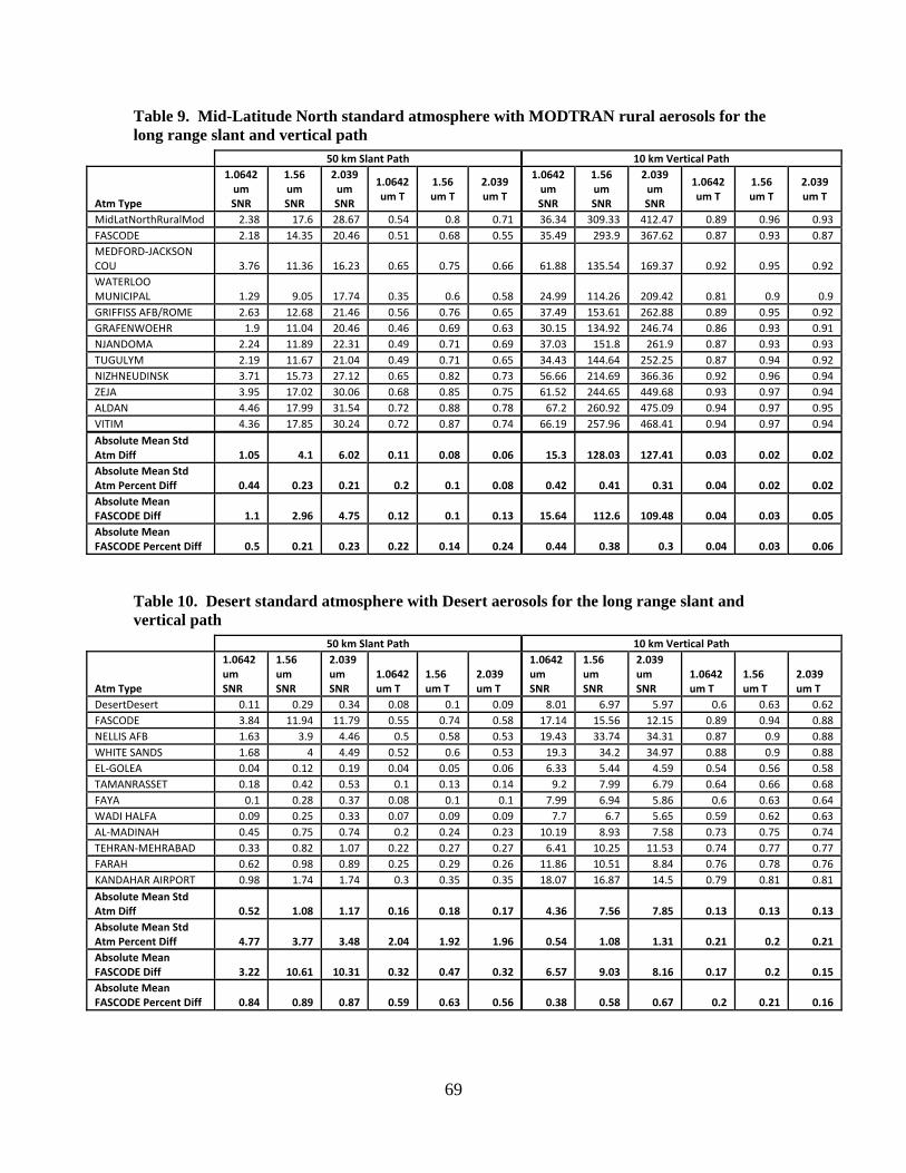
69
Table 9. Mid-Latitude North standard atmosphere with MODTRAN rural aerosols for the long range slant and vertical path
50 km Slant Path 10 km Vertical Path
Atm Type
1.0642 um SNR
1.56 um SNR
2.039 um SNR
1.0642 um T
1.56 um T
2.039 um T
1.0642 um SNR
1.56 um SNR
2.039 um SNR
1.0642 um T
1.56 um T
2.039 um T
MidLatNorthRuralMod 2.38 17.6 28.67 0.54 0.8 0.71 36.34 309.33 412.47 0.89 0.96 0.93
FASCODE 2.18 14.35 20.46 0.51 0.68 0.55 35.49 293.9 367.62 0.87 0.93 0.87
MEDFORD‐JACKSON COU 3.76 11.36 16.23 0.65 0.75 0.66 61.88 135.54 169.37 0.92 0.95 0.92
WATERLOO MUNICIPAL 1.29 9.05 17.74 0.35 0.6 0.58 24.99 114.26 209.42 0.81 0.9 0.9
GRIFFISS AFB/ROME 2.63 12.68 21.46 0.56 0.76 0.65 37.49 153.61 262.88 0.89 0.95 0.92
GRAFENWOEHR 1.9 11.04 20.46 0.46 0.69 0.63 30.15 134.92 246.74 0.86 0.93 0.91
NJANDOMA 2.24 11.89 22.31 0.49 0.71 0.69 37.03 151.8 261.9 0.87 0.93 0.93
TUGULYM 2.19 11.67 21.04 0.49 0.71 0.65 34.43 144.64 252.25 0.87 0.94 0.92
NIZHNEUDINSK 3.71 15.73 27.12 0.65 0.82 0.73 56.66 214.69 366.36 0.92 0.96 0.94
ZEJA 3.95 17.02 30.06 0.68 0.85 0.75 61.52 244.65 449.68 0.93 0.97 0.94
ALDAN 4.46 17.99 31.54 0.72 0.88 0.78 67.2 260.92 475.09 0.94 0.97 0.95
VITIM 4.36 17.85 30.24 0.72 0.87 0.74 66.19 257.96 468.41 0.94 0.97 0.94
Absolute Mean Std Atm Diff 1.05 4.1 6.02 0.11 0.08 0.06 15.3 128.03 127.41 0.03 0.02 0.02
Absolute Mean Std Atm Percent Diff 0.44 0.23 0.21 0.2 0.1 0.08 0.42 0.41 0.31 0.04 0.02 0.02
Absolute Mean FASCODE Diff 1.1 2.96 4.75 0.12 0.1 0.13 15.64 112.6 109.48 0.04 0.03 0.05
Absolute Mean FASCODE Percent Diff 0.5 0.21 0.23 0.22 0.14 0.24 0.44 0.38 0.3 0.04 0.03 0.06
Table 10. Desert standard atmosphere with Desert aerosols for the long range slant and vertical path
50 km Slant Path 10 km Vertical Path
Atm Type
1.0642 um SNR
1.56 um SNR
2.039 um SNR
1.0642 um T
1.56 um T
2.039 um T
1.0642 um SNR
1.56 um SNR
2.039 um SNR
1.0642 um T
1.56 um T
2.039 um T
DesertDesert 0.11 0.29 0.34 0.08 0.1 0.09 8.01 6.97 5.97 0.6 0.63 0.62
FASCODE 3.84 11.94 11.79 0.55 0.74 0.58 17.14 15.56 12.15 0.89 0.94 0.88
NELLIS AFB 1.63 3.9 4.46 0.5 0.58 0.53 19.43 33.74 34.31 0.87 0.9 0.88
WHITE SANDS 1.68 4 4.49 0.52 0.6 0.53 19.3 34.2 34.97 0.88 0.9 0.88
EL‐GOLEA 0.04 0.12 0.19 0.04 0.05 0.06 6.33 5.44 4.59 0.54 0.56 0.58
TAMANRASSET 0.18 0.42 0.53 0.1 0.13 0.14 9.2 7.99 6.79 0.64 0.66 0.68
FAYA 0.1 0.28 0.37 0.08 0.1 0.1 7.99 6.94 5.86 0.6 0.63 0.64
WADI HALFA 0.09 0.25 0.33 0.07 0.09 0.09 7.7 6.7 5.65 0.59 0.62 0.63
AL‐MADINAH 0.45 0.75 0.74 0.2 0.24 0.23 10.19 8.93 7.58 0.73 0.75 0.74
TEHRAN‐MEHRABAD 0.33 0.82 1.07 0.22 0.27 0.27 6.41 10.25 11.53 0.74 0.77 0.77
FARAH 0.62 0.98 0.89 0.25 0.29 0.26 11.86 10.51 8.84 0.76 0.78 0.76
KANDAHAR AIRPORT 0.98 1.74 1.74 0.3 0.35 0.35 18.07 16.87 14.5 0.79 0.81 0.81
Absolute Mean Std Atm Diff 0.52 1.08 1.17 0.16 0.18 0.17 4.36 7.56 7.85 0.13 0.13 0.13
Absolute Mean Std Atm Percent Diff 4.77 3.77 3.48 2.04 1.92 1.96 0.54 1.08 1.31 0.21 0.2 0.21
Absolute Mean FASCODE Diff 3.22 10.61 10.31 0.32 0.47 0.32 6.57 9.03 8.16 0.17 0.2 0.15
Absolute Mean FASCODE Percent Diff 0.84 0.89 0.87 0.59 0.63 0.56 0.38 0.58 0.67 0.2 0.21 0.16

70
Table 11. Tropical standard atmosphere with maritime tropical aerosols for the long range slant and vertical path
50 km Slant Path 10 km Vertical Path
Atm Type
1.0642 um SNR
1.56 um SNR
2.039 um SNR
1.0642 um T
1.56 um T
2.039 um T
1.0642 um SNR
1.56 um SNR
2.039 um SNR
1.0642 um T
1.56 um T
2.039 um T
TropicalMaritimeTropical 0.35 0.74 0.78 0.2 0.26 0.22 5.82 8.15 8.8 0.73 0.77 0.74
FASCODE 0.87 1.69 1.8 0.33 0.41 0.34 6.99 9.59 10.01 0.8 0.83 0.79
LIHUE/KAUAI ISLAND 0.19 0.43 0.41 0.12 0.13 0.09 3.7 6.17 6.42 0.66 0.67 0.63
PAGO PAGO/INT.AIRP. 0.29 0.57 0.47 0.19 0.21 0.13 4.1 6.75 7.03 0.72 0.73 0.67
GUANTANAMO BAY NAS 1.01 2.41 2.21 0.29 0.34 0.23 13.8 22.42 21.94 0.79 0.81 0.75
SAN JUAN INTL ARPT 0.63 1.39 1.16 0.25 0.28 0.18 8.34 13.69 12.95 0.76 0.78 0.72
BERMUDA INTERNATION 0.48 1.06 0.99 0.25 0.28 0.21 5.97 10.33 10.91 0.76 0.78 0.73
GRANTLEY ADAMS 0.3 0.62 0.51 0.17 0.19 0.12 4.76 7.69 7.56 0.71 0.72 0.66
LAJES (ACORES) 0.26 0.58 0.61 0.16 0.18 0.15 4.2 7.04 7.56 0.7 0.71 0.68
SEYCHELLES INTERNAT 0.38 0.74 0.61 0.24 0.26 0.16 4.76 7.88 8.26 0.75 0.77 0.7
DIEGO GARCIA 0.3 0.6 0.5 0.2 0.21 0.13 4.22 6.96 7.26 0.73 0.74 0.67
KWAJALEIN/BUCHOLZ A 0.38 0.76 0.62 0.24 0.26 0.16 4.84 8.02 8.35 0.75 0.76 0.69
Absolute Mean Std Atm Diff 0.15 0.36 0.37 0.04 0.05 0.07 2.08 2.85 2.85 0.03 0.03 0.05
Absolute Mean Std Atm Percent Diff 0.44 0.48 0.48 0.21 0.19 0.3 0.36 0.35 0.32 0.04 0.04 0.07
Absolute Mean FASCODE Diff 0.48 0.92 1.07 0.11 0.17 0.18 2.75 3.43 3.34 0.06 0.09 0.1
Absolute Mean FASCODE Percent Diff 0.55 0.54 0.6 0.35 0.43 0.54 5.82 8.15 8.8 0.73 0.77 0.74
The short range geometries in desert environments, Table 6, clearly show that
both the signal-to-noise ratios and the transmissions are lower than for the previous two
tables. As discussed earlier, desert environments provide the ideal scenario in which dust
can be lifted into the atmosphere. Deserts have loose fine particles in the 50 to 200 μm
range and regularly have surface winds above 0.2 m/s meeting the criterion to inject dust
into the atmosphere. Desert regions are the atmosphere's main source of suspended dust
particles (Wallace and Hobbs 2006). Unlike the mid-latitude standard profiles,
transmissions are very strongly correlated to the signal-to-noise for the desert climate.
Faya, Chad has the same transmission as the standard atmosphere with a value of 0.63.
Interestingly, their signal-to-noise ratios also exactly match. This can be explained from
the fact that the major difference between the ExPERT atmospheres and the standard
atmospheres is the allowance of aerosols to swell with height. In desert environments,

71
the air is so dry that there is not enough moisture in the air for this to happen, and hence
the standard and ExPERT profiles will look very similar. The composition of absorption
and scattering due to molecules and aerosols will also be similar as desert aerosols have
very little absorption.
In Table 8 the long range urban standard atmosphere, there was great dissimilarity
from the ExPERT atmospheres for the 1.0642 μm wavelength being on average almost
73 times too small. That is a 7300 percent difference. Surprisingly, at the 2.039 μm
wavelength, there was a great reduction in this number to a mean percent difference of
77. Of the locations analyzed, Shanghai, China had the worst transmissions and signal-
to-noise ratios. The long range rural signal-to-noise ratios again are larger than the urban
case. The standard atmosphere is tolerable in characterizing the ExPERT sites for this
case, having a mean percent difference of about 20 for the two longer wavelengths. In
Table 10, the long range desert climate assessments, the transmissions are once again
very well correlated to the signal-to-noise ratios for both the slant and the vertical
geometries. In the last chart, the long range tropical environments, the mean standard
percent difference remained nearly constant across the three wavelengths for both the
slant and vertical geometries. This was a result of the profiles scaling the same between
the different wavelengths. Because the maritime tropical aerosols are mainly sea salt,
this showed that both the standard atmosphere and the ExPERT atmosphere scaled these
aerosols very nearly the same, though the ExPERT atmosphere let them swell with
altitude.
The transmission does not always correlate to the signal-to-noise ratio. This is
demonstrated by looking at the 2.039 μm wavelength 3 km urban signal-to-noise values

72
in Figure 18. The plots display the effect the uncorrelated noise for various atmosphere
profiles have on the signal-to-noise ratio. Because the noise is uncorrelated for various
atmosphere profiles, the signal-to-noise ratio is likewise uncorrelated. The shorter two
wavelengths shows a similar uncorrelation to a lesser extent. The main cause for signal-
to-noise not to be correlated is that different atmospheric profiles have different
absorption and scattering profiles. The absorption causes a loss of transmission with no
increased noise, while scattering causes a loss of transmission and an increase in noise.
Transmission will correlate with signal-to-noise ratios for profiles in which there
is no absorption. Desert environment profiles have virtually no absorption and there is
very little difference within the boundary layer because desert aerosols are not
hygroscopic. Because of the noise correlation as seen in Figure 19 the signal-to-noise
was also correlated. The FASCODE values did not correlate because the signal was
produced using the FASCODE transmissions while the noise was calculated from the
Figure 18. Signal-to-noise ratio correlation at 2.039 μm wavelength 3 km range for the Mid-Latitude North urban simulations. From left to right is the signal, noise, and signal-to-noise plotted against transmission. The x marks the standard profile value and the o marks the FASCODE value.
0.5 0.55 0.6 0.65 0.7 0.75 0.8 0.85 0.90.015
0.02
0.025
0.03
0.035
0.04
0.045
Transmission
Sig
nal (
W/m
2 )
0.5 0.55 0.6 0.65 0.7 0.75 0.8 0.85 0.90.2
0.4
0.6
0.8
1
1.2
1.4
1.6
1.8
2x 10
-4
Transmission
Noi
se (
W/m
2 )
0.5 0.55 0.6 0.65 0.7 0.75 0.8 0.85 0.90
500
1000
1500
Transmission
SN
R (
W/m
2 )
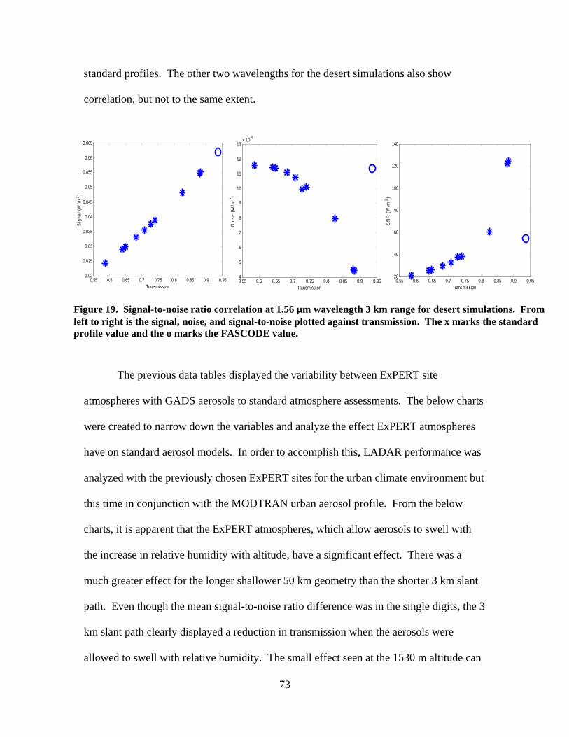
73
standard profiles. The other two wavelengths for the desert simulations also show
correlation, but not to the same extent.
The previous data tables displayed the variability between ExPERT site
atmospheres with GADS aerosols to standard atmosphere assessments. The below charts
were created to narrow down the variables and analyze the effect ExPERT atmospheres
have on standard aerosol models. In order to accomplish this, LADAR performance was
analyzed with the previously chosen ExPERT sites for the urban climate environment but
this time in conjunction with the MODTRAN urban aerosol profile. From the below
charts, it is apparent that the ExPERT atmospheres, which allow aerosols to swell with
the increase in relative humidity with altitude, have a significant effect. There was a
much greater effect for the longer shallower 50 km geometry than the shorter 3 km slant
path. Even though the mean signal-to-noise ratio difference was in the single digits, the 3
km slant path clearly displayed a reduction in transmission when the aerosols were
allowed to swell with relative humidity. The small effect seen at the 1530 m altitude can
Figure 19. Signal-to-noise ratio correlation at 1.56 μm wavelength 3 km range for desert simulations. From left to right is the signal, noise, and signal-to-noise plotted against transmission. The x marks the standard profile value and the o marks the FASCODE value.
0.55 0.6 0.65 0.7 0.75 0.8 0.85 0.9 0.950.02
0.025
0.03
0.035
0.04
0.045
0.05
0.055
0.06
0.065
Transmission
Sig
nal (
W/m
2 )
0.55 0.6 0.65 0.7 0.75 0.8 0.85 0.9 0.954
5
6
7
8
9
10
11
12
13x 10
-4
Transmission
Noi
se (
W/m
2 )
0.55 0.6 0.65 0.7 0.75 0.8 0.85 0.9 0.9520
40
60
80
100
120
140
Transmission
SN
R (
W/m
2 )

74
be explained from the fact that the 10% gate starts at 153 m above the ground where both
the ExPERT and standard profiles are nearly identical. The total transmission has little
effect on the signal-to-noise ratio as can be seen from Pyongyang, which has only a 7%
transmission, yet only a slightly lower signal-to-noise ratio than the standard profile.
Table 12. North standard atmosphere with MODTRAN urban aerosols for the short range slant and vertical path
3 km Slant Path 1530 m Vertical Path
Atm Type
1.0642 um SNR
1.56 um SNR
2.039 um SNR
1.0642 um T
1.56 um T
2.039 um T
1.0642 um SNR
1.56 um SNR
2.039 um SNR
1.0642 um T
1.56 um T
2.039 um T
MidLatNorthUrbanMod 116.54 361.95 889.31 0.4 0.62 0.71 240.46 729.22 1779.63 0.63 0.78 0.84
FASCODE 101.76 280.28 628.19 0.38 0.54 0.6 224.8 640.17 1486.07 0.61 0.73 0.77
PITTSBURGH/GREATER 124.97 397.23 827.24 0.23 0.46 0.6 259.52 801.66 1656.2 0.47 0.67 0.77
CAMP SPRINGS/ANDREW 123.35 392.98 823.83 0.21 0.44 0.59 256.57 793.18 1649.4 0.45 0.66 0.76
BOSTON/LOGAN INTL 116.24 374.68 835.83 0.12 0.33 0.5 246.27 756.93 1672.03 0.34 0.56 0.7
LONDON/HEATHROW AIR 120.35 385.09 824.06 0.16 0.38 0.55 251.86 777.57 1648.72 0.39 0.61 0.74
PARIS‐ORLY 124.56 396.38 825.13 0.23 0.47 0.61 258.58 799.92 1652.36 0.47 0.68 0.77
LUXEMBOURG/LUXEMBOU 123.61 393.63 826.06 0.2 0.43 0.58 257.34 794.58 1653.19 0.44 0.65 0.76
ZURICH‐KLOTEN 125.14 397.5 827.58 0.23 0.46 0.61 259.82 802.22 1657.02 0.47 0.68 0.77
KYIV 121 386.51 824.39 0.17 0.39 0.55 252.92 780.36 1649.5 0.4 0.62 0.74
SHANGHAI/HONGQIAO 107.09 354.16 883.81 0.08 0.26 0.42 235.75 716.5 1773.63 0.27 0.5 0.64
PYONGYANG 104.05 350.03 890.63 0.07 0.24 0.41 233.22 708.58 1783.85 0.25 0.48 0.64
Absolute Mean Std Atm Diff 6.94 24.81 50.72 0.23 0.23 0.17 13.11 50.61 100.88 0.23 0.17 0.11
Absolute Mean Std Atm Percent Diff 0.06 0.07 0.06 0.58 0.38 0.24 0.05 0.07 0.06 0.37 0.22 0.13
Absolute Mean FASCODE Diff 17.28 102.54 210.67 0.21 0.16 0.06 26.39 132.98 193.52 0.21 0.12 0.04
Absolute Mean FASCODE Percent Diff 0.17 0.37 0.34 0.55 0.29 0.1 0.12 0.21 0.13 0.35 0.17 0.05
Table 13 shows a much larger contrast because of the longer distance traveled
through the region of the atmosphere in which the aerosols have swelled. As seen in the
table, this almost reduces the signal-to-noise ratio in half for the 50 km 1.0642 μm case.
The larger effect at the 10 km altitude can be explained from the 10% gate starting at 1
km, near the bottom of the spike in the ExPERT atmosphere. The difference between the
two atmosphere transmissions are also much larger. The numbers are coming out to zero
for some columns because all numbers in the charts were truncated to two decimal places

75
for displaying purposes.
Table 13. North standard atmosphere with MODTRAN urban aerosols for the long range slant and vertical path
50 km Slant Path 10 km Vertical Path
Atm Type
1.0642 um SNR
1.56 um SNR
2.039 um SNR
1.0642 um T
1.56 um T
2.039 um T
1.0642 um SNR
1.56 um SNR
2.039 um SNR
1.0642 um T
1.56 um T
2.039 um T
MidLatNorthUrbanMod 0.02 1.49 9.42 0.02 0.14 0.24 25.36 88.69 220.81 0.48 0.68 0.75
FASCODE 0.12 2.41 7.65 0.07 0.18 0.21 35.95 96.48 201.63 0.57 0.71 0.72
PITTSBURGH/GREATER 0 0.37 5.42 0 0.06 0.15 21.52 77.82 198.54 0.35 0.57 0.69
CAMP SPRINGS/ANDREW 0 0.29 4.77 0 0.05 0.14 20.63 74.89 195.39 0.33 0.56 0.68
BOSTON/LOGAN INTL 0 0.07 2.44 0 0.03 0.09 13.66 50.57 155.85 0.25 0.48 0.63
LONDON/HEATHROW AIR 0 0.15 3.63 0 0.04 0.12 18.01 66.08 184.38 0.29 0.52 0.65
PARIS‐ORLY 0 0.38 5.33 0 0.06 0.15 21.54 77.99 198.12 0.35 0.58 0.69
LUXEMBOURG/LUXEMBOU 0 0.26 4.75 0 0.05 0.14 20.39 74.09 195.17 0.32 0.55 0.68
ZURICH‐KLOTEN 0 0.38 5.48 0 0.06 0.15 21.6 78.07 198.72 0.35 0.58 0.69
KYIV 0 0.17 3.84 0 0.04 0.12 18.5 67.69 186.87 0.3 0.53 0.66
SHANGHAI/HONGQIAO 0 0.02 0.6 0 0.01 0.06 2.7 9.68 23.94 0.2 0.43 0.57
PYONGYANG 0 0.01 0.5 0 0.01 0.06 1.95 7.12 17.62 0.19 0.42 0.57
Absolute Mean Std Atm Diff 0.01 1.28 5.74 0.02 0.1 0.12 9.31 30.29 65.35 0.18 0.15 0.1
Absolute Mean Std Atm Percent Diff 0.98 0.86 0.61 0.89 0.7 0.5 0.37 0.34 0.3 0.39 0.23 0.14
Absolute Mean FASCODE Diff 0.12 2.2 3.98 0.06 0.14 0.09 19.9 38.07 46.17 0.28 0.18 0.07
Absolute Mean FASCODE Percent Diff 1 0.91 0.52 0.96 0.77 0.44 0.55 0.39 0.23 0.49 0.26 0.09
Figure 20 displays the atmospheric profiles for both the standard and the ExPERT
atmosphere with MODTRAN urban aerosols. The scale was kept constant for an easy
comparison. The spike at about 1500 m, also known as the Fiorino spike, in the Expert
atmosphere plots are due to the swelling of aerosols with the increase in relative humidity
at the top of the atmosphere. While aerosol scattering decreases in the standard
atmosphere at the two longer wavelengths, allowing aerosol absorption to become the
major extinction constituent, aerosol scattering remains the number one extinction factor
in the ExPERT profiles for all three wavelengths.
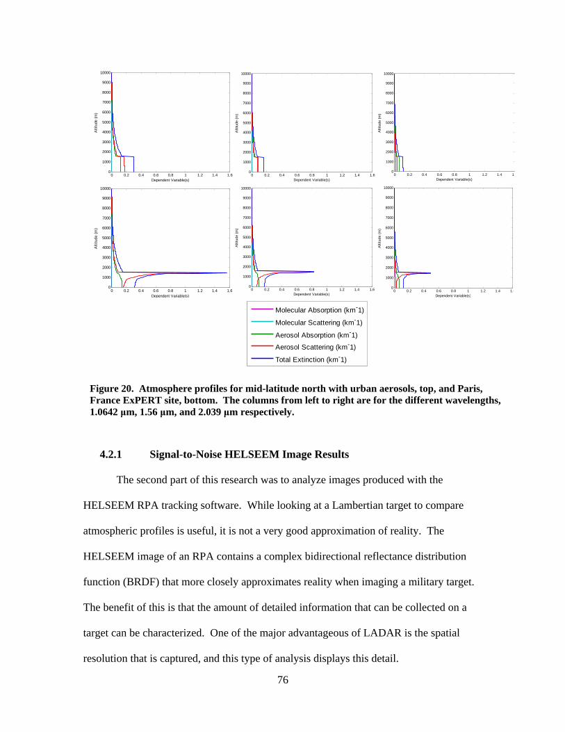
76
4.2.1 Signal-to-Noise HELSEEM Image Results
The second part of this research was to analyze images produced with the
HELSEEM RPA tracking software. While looking at a Lambertian target to compare
atmospheric profiles is useful, it is not a very good approximation of reality. The
HELSEEM image of an RPA contains a complex bidirectional reflectance distribution
function (BRDF) that more closely approximates reality when imaging a military target.
The benefit of this is that the amount of detailed information that can be collected on a
target can be characterized. One of the major advantageous of LADAR is the spatial
resolution that is captured, and this type of analysis displays this detail.
Figure 20. Atmosphere profiles for mid-latitude north with urban aerosols, top, and Paris, France ExPERT site, bottom. The columns from left to right are for the different wavelengths, 1.0642 μm, 1.56 μm, and 2.039 μm respectively.
0 0.2 0.4 0.6 0.8 1 1.2 1.4 1.60
1000
2000
3000
4000
5000
6000
7000
8000
9000
10000
Alti
tude
(m
)
Dependent Variable(s)
0 0.2 0.4 0.6 0.8 1 1.2 1.4 1.60
1000
2000
3000
4000
5000
6000
7000
8000
9000
10000
Alti
tude
(m
)
Dependent Variable(s)
0 0.2 0.4 0.6 0.8 1 1.2 1.4 10
1000
2000
3000
4000
5000
6000
7000
8000
9000
10000
Alti
tude
(m
)
Dependent Variable(s)
0 0.2 0.4 0.6 0.8 1 1.2 1.4 1.60
1000
2000
3000
4000
5000
6000
7000
8000
9000
10000
Alti
tude
(m
)
Dependent Variable(s)
0 0.2 0.4 0.6 0.8 1 1.2 1.4 1.60
1000
2000
3000
4000
5000
6000
7000
8000
9000
10000
Alti
tude
(m
)
Dependent Variable(s)
0 0.2 0.4 0.6 0.8 1 1.2 1.4 1.60
1000
2000
3000
4000
5000
6000
7000
8000
9000
10000
Alti
tude
(m
)
Dependent Variable(s)
Molecular Absorption (km-1)
Molecular Scattering (km-1)
Aerosol Absorption (km-1)
Aerosol Scattering (km-1)
Total Extinction (km-1)
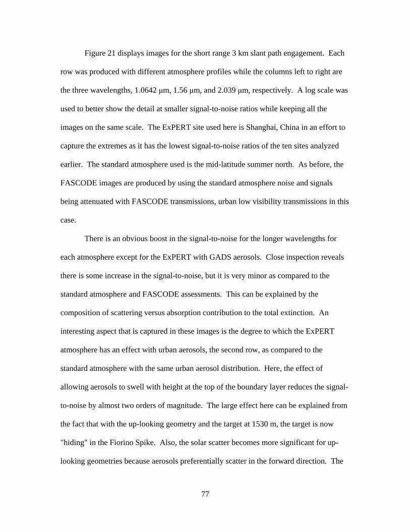
77
Figure 21 displays images for the short range 3 km slant path engagement. Each
row was produced with different atmosphere profiles while the columns left to right are
the three wavelengths, 1.0642 μm, 1.56 μm, and 2.039 μm, respectively. A log scale was
used to better show the detail at smaller signal-to-noise ratios while keeping all the
images on the same scale. The ExPERT site used here is Shanghai, China in an effort to
capture the extremes as it has the lowest signal-to-noise ratios of the ten sites analyzed
earlier. The standard atmosphere used is the mid-latitude summer north. As before, the
FASCODE images are produced by using the standard atmosphere noise and signals
being attenuated with FASCODE transmissions, urban low visibility transmissions in this
case.
There is an obvious boost in the signal-to-noise for the longer wavelengths for
each atmosphere except for the ExPERT with GADS aerosols. Close inspection reveals
there is some increase in the signal-to-noise, but it is very minor as compared to the
standard atmosphere and FASCODE assessments. This can be explained by the
composition of scattering versus absorption contribution to the total extinction. An
interesting aspect that is captured in these images is the degree to which the ExPERT
atmosphere has an effect with urban aerosols, the second row, as compared to the
standard atmosphere with the same urban aerosol distribution. Here, the effect of
allowing aerosols to swell with height at the top of the boundary layer reduces the signal-
to-noise by almost two orders of magnitude. The large effect here can be explained from
the fact that with the up-looking geometry and the target at 1530 m, the target is now
"hiding" in the Fiorino Spike. Also, the solar scatter becomes more significant for up-
looking geometries because aerosols preferentially scatter in the forward direction. The

78
ExPERT atmosphere scattering aerosols greatly raise the noise, keeping the signal-to-
noise ratio low for all three wavelengths. The standard profile does not have this spike,
allowing the signal-to-noise ratio to be much larger.
Table 14 displays the total path noise components in irradiance units of watts per
meter squared for the 3 km slant path for the ExPERT Shanghai, China and the standard
Figure 21. Short range 3 km slant path image signal-to-noise ratios. The platform is on the ground looking up at a 1530 m altitude target.
Expert Atm
GADS
Aerosols
Expert Atm
Urban
Aerosols
Std Atm
Urban
Aerosols
Std Atm
Urban
Aerosls FA
SCODE
Trans
1.06 μm 1.56 μm 2.04 μm
1
2
5
10
20
50
100
200
500
1000

79
atmosphere profile. The major difference between the two is the laser scatter being two
orders of magnitude larger for the ExPERT atmosphere. The solar scatter is also much
larger, being about one order of magnitude larger. The solar reflection is not included
here as it was computed with HELSEEM and merely subtracted from the plane signature.
Table 14. Composition of noise components for the 3 km slant path geometry
ExPERT Background Laser Scatter Solar Scatter Black Body Transmission
1.0642 μm 2.98E‐05 1.937E‐3 1.6E‐4 3.69E‐17 0.469779
1.56 μm 1.01E‐05 1.565E‐3 5.55E‐05 1.05E‐11 0.546315
2.039 μm 4.44E‐06 8.33E‐4 1.75E‐05 3.72E‐09 0.537467
Std Atm
1.0642 μm 3.36E‐05 9.15E‐05 8.11E‐05 3.17E‐17 0.403737
1.56 μm 1.13E‐05 6.91E‐05 1.94E‐05 1.19E‐11 0.616893
2.039 μm 2.08E‐06 2.95E‐05 3.23E‐06 4.92E‐09 0.711559
Figure 22 is the signal-to-noise images for the 50 km up-looking engagement.
The images are produced exactly the same way as Figure 21, except for the longer range
geometry and the scale has been reduced to have a maximum value of 100. In this
scenario, the increase in the signal-to-noise for the ExPERT atmosphere with GADS
aerosols with the increase in wavelength is very apparent. At the 1.0642 μm wavelength,
very little shows up above the noise besides the normal facing stripe on the fuselage and
the front tail strut of the RPA for every atmosphere except for the ExPERT with urban
aerosols, in which case the plane is not visible at all. There is a drastic difference
displayed in this scenario between the standard atmosphere with urban aerosols and the
ExPERT atmosphere with urban aerosols. In fact, for both the 1.0642 μm and the 1.56
μm wavelength ExPERT atmosphere with urban aerosols image, no information can be
gained about the plane. There is also a noticeable difference between the standard

80
atmosphere and the FACODE images at the 1.56 μm wavelength. The FASCODE
transmission is clearly less than that of the standard profile, causing lower signal-to-noise
ratios. The large difference between the ExPERT and standard profile images can once
again be explained from the aerosol spike at the top of the boundary layer. Although the
gate is far above the spike, solar scattering noise, which is the dominate noise source for
the long range scenario, comes from scattering over the entire path. The difference
between the up-looking images in Figure 22, and the smaller effect previously seen in the
long range down looking tables can be explained by the fact that the aerosol spike is now
much closer to the receiver with much less distance to disperse.
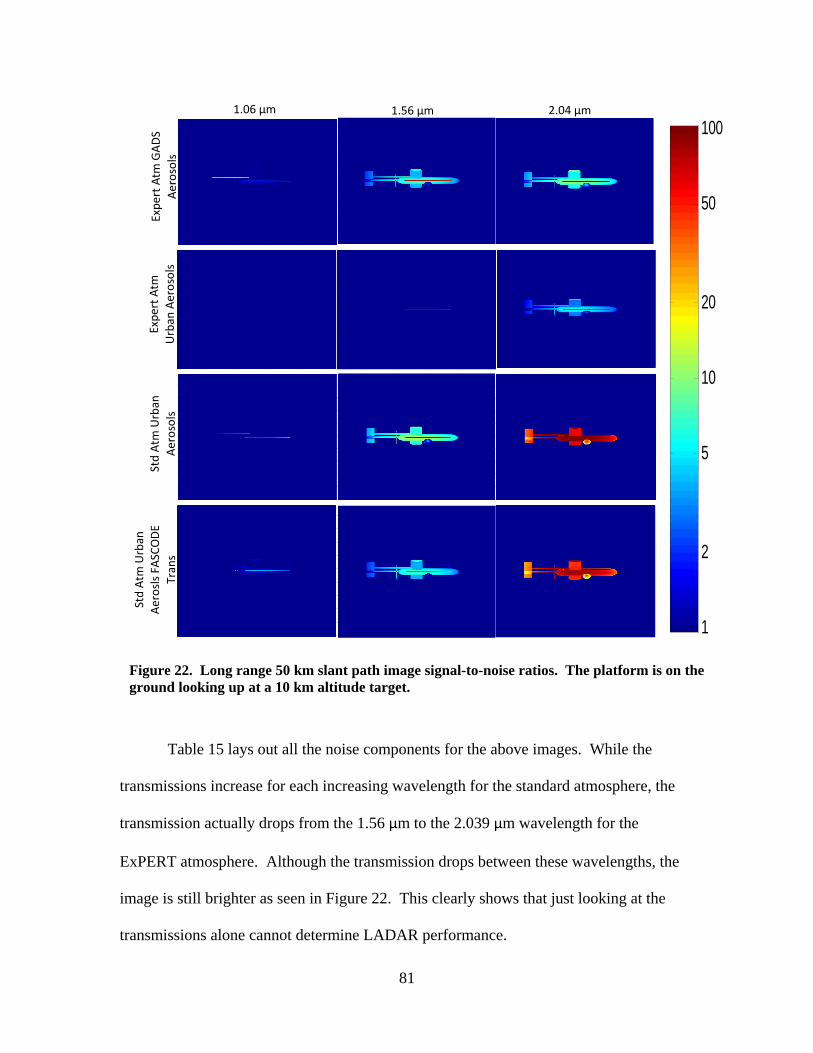
81
Table 15 lays out all the noise components for the above images. While the
transmissions increase for each increasing wavelength for the standard atmosphere, the
transmission actually drops from the 1.56 μm to the 2.039 μm wavelength for the
ExPERT atmosphere. Although the transmission drops between these wavelengths, the
image is still brighter as seen in Figure 22. This clearly shows that just looking at the
transmissions alone cannot determine LADAR performance.
Figure 22. Long range 50 km slant path image signal-to-noise ratios. The platform is on the ground looking up at a 10 km altitude target.
Expert Atm
GADS
Aerosols
Expert Atm
Urban
Aerosols
Std Atm
Urban
Aerosols
Std Atm
Urban
Aerosls FA
SCODE
Trans
1.06 μm 1.56 μm 2.04 μm
1
2
5
10
20
50
100

82
Table 15. Composition of noise components for the 50 km slant path geometry
ExPERT Background Laser Scatter Solar Scatter Black Body Transmission
1.0642 μm 8.34E‐08 2.00E‐08 7.29E‐06 4.44E‐19 0.094184
1.56 μm 5.43E‐08 1.73E‐08 2.62E‐06 1.85E‐13 0.160024
2.039 μm 1.39E‐07 6.94E‐09 7.66E‐07 5.94E‐11 0.143053
Std Atm
1.0642 μm 1.71E‐08 1.10E‐09 3.57E‐06 1.12E‐19 0.023753
1.56 μm 1.10E‐08 8.27E‐09 1.19E‐06 1.60E‐13 0.138791
2.039 μm 3.19E‐09 8.32E‐09 2.22E‐07 9.85E‐11 0.237333
Figure 23 explains why just looking at the transmissions alone is unable to predict
the signal-to-noise ratio. By looking at the profiles, why the signal-to-noise ratio goes off
the charts for the standard atmosphere while increasing at a much smaller rate for the
ExPERT atmosphere can be seen. Notice at the two longer wavelengths that aerosol
absorption becomes the major extinction constituent for the standard atmosphere profiles
while scattering remains extremely high in the ExPERT profile with very little
contribution from absorption. This is important because the noise seen by the Geiger
mode LADAR system is due to scattering. Therefore, two profiles could have exactly the
same transmission while the signal-to-noise ratios could differ greatly. The scales are
changed from plot to plot so the contributions to extinction from the different parameters
could be identified.

83
While analyzing atmospheric effects on LADAR signatures, atmospheric
turbulence cannot be ignored. While turbulence will not affect the actual signal-to-noise
ratio, it will affect what information can be obtained from the target. Figure 24 is created
using the climatological wind and turbulence profiles at the 50th percentile in LEEDR.
Figure 23. Atmosphere profiles for Shanghai ExPERT with GADS aerosols, Shanghai ExPERT with urban aerosols, and mid-latitude north with urban aerosols from top to bottom. The columns left to right are for the three wavelengths, 1.0642 μm, 1.56 μm, and 2.039 μm respectively. The plots have the extinction coefficient values (km-1) along the x axis and altitude (m) along the y axis.
0 0.05 0.1 0.15 0.2 0.25 0.3 0.35 0.4 0.450
200
400
600
800
1000
1200
1400
1600
Alti
tude
(m
)
Dependent Variable(s)
0 0.05 0.1 0.15 0.2 0.25 0.3 0.35 0.40
200
400
600
800
1000
1200
1400
1600
Alti
tude
(m
)
Dependent Variable(s)
0 0.05 0.1 0.15 0.2 0.25 0.3 0.350
200
400
600
800
1000
1200
1400
1600
Dependent Variable(s)
Alti
tude
(m
)
0 0.5 1 1.50
200
400
600
800
1000
1200
1400
1600
Alti
tude
(m
)
Dependent Variable(s)
0 0.1 0.2 0.3 0.4 0.5 0.6 0.7 0.80
200
400
600
800
1000
1200
1400
1600
Alti
tude
(m
)
Dependent Variable(s)
0 0.05 0.1 0.15 0.2 0.25 0.3 0.35 0.4 0.45 0.50
200
400
600
800
1000
1200
1400
1600
Alti
tude
(m
)
Dependent Variable(s)
0 0.05 0.1 0.15 0.2 0.25 0.3 0.350
200
400
600
800
1000
1200
1400
1600
Alti
tude
(m
)
Dependent Variable(s)
0 0.02 0.04 0.06 0.08 0.1 0.12 0.14 0.16 0.180
200
400
600
800
1000
1200
1400
1600
Alti
tude
(m
)
Dependent Variable(s)
0 0.02 0.04 0.06 0.08 0.1 0.120
200
400
600
800
1000
1200
1400
1600
Alti
tude
(m
)
Dependent Variable(s)
Molecular Absorption (km-1)
Molecular Scattering (km-1)
Aerosol Absorption (km-1)
Aerosol Scattering (km-1)
Total Extinction (km-1)

84
Turbulence has very little effect on the 3 km slant range, but has a drastic effect on the 50
km slant range. In the 3 km slant path geometry images, fine detail about the RPA can be
identified, including the radar dome on its belly as well as the dimensions of various
components of the aircraft. At the 50 km range, all detail of the plane as been blurred, to
the point it is hard to even tell if it is an airplane.
4.3 Summary
The global signal-to-noise ratios computed using LEEDR atmospheres revealed
how the signal-to-noise varied with wavelength, engagement geometry and climate.
While the standard profile characterizations many times provided satisfactory results in
describing the average LADAR performance in different atmospheric conditions, there is
strong variability between global locations despite having similar environments. This
Figure 24. ExPERT with GADS images with atmospheric turbulence effects. Top row is the 3 km slant path engagement while the bottom row is the 50 km slant path engagement. From left to right the columns are for the 1.0642 μm, 1.56 μm, and the 2.039 μm wavelength respectively.
1
2
5
10
20
50
100
200
500
1000
0.5
1
2
5
10
85
variability is better captured with the ExPERT atmospheres and GADS aerosols. The
signal-to-noise ratio and transmission are shown to not always correlate. Images of an
RPA displaying signal-to-noise in conjunction with atmosphere profiles reveal that the
correlation between signal-to-noise and transmission values is greatly dependent upon the
composition of the scattering and absorption of the extinction profiles. These images also
show that ignoring the aerosol spike at the top of the boundary layer leads to signal-to-
noise ratio values that can be several orders of magnitude too large being wavelength,
geometry, and gate location dependent.

86
V Conclusions and Recommendations
5.1 Chapter Overview
Current developers of LADAR systems do not have tools to accurately model
many propagation features of the atmosphere. The objective of this research is to
quantify the effect of using the more realistic LEEDR atmospheres versus a standard
atmosphere profile when simulating LADAR signal-to-noise ratios. This study shows
that accounting for location climatology and aerosol expansion at the top of the boundary
layer can cause orders of magnitude differences in signal-to-noise evaluations.
5.2 Conclusions of Research
Upon the onset of this research, the goal was to show the advantages of using a
probabilistic climatological approach to modeling atmospheric effects on LADAR
performance. From plotting global maps of signal-to-noise ratios computed using
ExPERT atmospheres with GADS aerosols, it is clear that the different climates give
different values. In fact, desert and maritime regions have signal-to-noise ratio values
orders of magnitude less than rural areas. This suggests that a standard profile with a
standard aerosol model may be able to capture these different regions of the earth.
However, after careful analysis by choosing various locations that should be adequately
described by a certain standard profile, significant differences are seen.
The differences are rooted in the fact that just because a specified location has a
certain type of climate, its atmosphere is still significantly different than a similar climate
at another location on the globe. For instance Wadi Halfa, Sudan and Nellis AFB,
Nevada from Table 4-5 can both be described as desert locations. However, Wadi Halfa

87
has a signal-to-noise ratio of 30.15 while Nellis has a signal-to-noise ratio of 72.81. The
standard atmosphere solution is 31.18. Using a standard atmosphere with a standard
profile gives a ballpark answer, but does not give the precision needed when evaluating
the performance of combat systems. For all the scenarios studied, the average absolute
mean percent difference in signal-to-noise ratios is 1.03, meaning the ExPERT site on
average gives a value with a difference of about the value of that of the standard profile.
Over all, a value of 0.34 for the equivalent transmission comparison is found. The
equivalent median signal-to-noise ratio and transmission values are 0.51 and 0.15
respectively. Surprisingly just using the FASCODE transmissions for the signal
generation reduces this value to 0.847. The biggest difference comes from the 50 km
slant path urban comparison at 1.0642 μm for which the ExPERT sites give signal-to-
noise ratios 72 times greater than that of the standard profile which is excluded from the
above statistics being an outlier.
Another significant result is the analysis of correlations between signal-to-noise
ratios and transmission values. There is clearly some correlation, but what really matters
is the composition of the total extinction profile between absorption and scattering.
Because scattered energy constitutes the largest noise component in the Geiger mode
LADAR system, more scattering means more noise. Therefore, two profiles can give the
same transmission, but significantly different signal-to-noise ratios. This is clearly seen
in the HELSEEM 3 km slant path for the 1.0642 μm wavelength as the transmission is
0.4 or 40% for the standard profile and 0.47 or 47% for the ExPERT profile, yet the
signal-to-noise in much of standard profile image is more than four times greater than
that of the ExPERT profile.

88
Another conclusion can be drawn from comparing the images produced with
urban aerosols, one with a Shanghai ExPERT atmosphere, and the others with the
standard profile. These images show that ignoring the swelling of aerosols with altitude
as the standard profile does leads to orders of magnitude differences in the signal-to-noise
ratio. Without factoring in the aerosol spike at the top of the boundary layer, it is
impossible to accurately model LADAR propagation that travels any significant distance
in this region.
5.3 Significance of Research
One important result of this research is that a method is developed by which
Geiger mode LADAR system environmental effects can be analyzed. Also, a technique
to compare different atmosphere profiles is shown. This sets the foundation from which
future research can be developed.
The variance of location climatology is significant enough that a single
atmospheric model for similar environments cannot effectively capture the effects on
LADAR systems. This research shows that if a standard profile is used to model
environmental effects on a Geiger mode LADAR system, the solution could be orders of
magnitude different from that of a probabilistic approach. Also, this study shows the
importance of allowing aerosol effects to increase at the top of the boundary layer where
they swell with relative humidity. Once again, the difference between allowing aerosols
to swell and failing to let them swell was a couple orders of magnitude in the signal-to-
noise ratio. This investigation also shows that not only is the total transmission important
in determining the signal-to-noise, but also the composition of total extinction between
absorption and scattering.

89
The engagement geometries studied show some interesting employment
techniques that could both be used to exploit and defeat the environmental conditions.
As expected, longer engagement geometries cause lower signal-to-noise ratios, but more
significant was the atmospheric turbulence effects. To capture useful data at high
altitudes, it is expected that near vertical geometries are required or the employment of
adaptive optics techniques. An even more fascinating result is that ground LADAR
systems will have a much lower signal-to-noise ratio for targets flying at the top of the
boundary layer where aerosol scattering is maximized. The aerosol spike could
effectively be used to hide small RPAs from ground based LADARs.
LADAR is an emerging technology, and as systems are built, it is important to
understand their performance in certain environments. If atmospheric effects are deemed
insignificant on the system because of a study done using a standard atmosphere, actual
experimental data may yield a completely different analysis. Using a climatological
approach in modeling these systems will better capture the effects various atmosphere
types around the world will have on the system. With this knowledge, developers will be
able to better tailor the system to the type of environment in which it is expected to
operate.
5.4 Recommendations for Future Research
The results show that there is significant variance between a climatological and a
standard profile approach. However, how more accurate the climatological approach is,
or if it is even more accurate, is not studied. An analysis against real LADAR system
signal-to-noise high fidelity data at various locations would be an appropriate way to
determine the validity of the probabilistic atmosphere approach. Another way to validate

90
the probabilistic approach would be to leave the LADAR system out of the equation, and
do an in-depth analysis and validation of the ExPERT atmosphere profiles with GADS
aerosols.
This research only focused on the environmental effects and therefore did not
consider different real-world LADAR detectors. By analyzing an actual detector's
capability, the signal-to-noise ratios could be tailored to determine if signals would be
detected for that system. This type of analysis could be done at a specified location and
then compared to experimental data. A major simplification is taken in the probability of
detection versus false alarm analysis as only a single pulse scenario is examined. To
better characterize the detectability of a particular system, a statistical analysis would
need to be accomplished. Some LADAR systems operate as a continuous wave instead
of distinct pulses. Some of the analysis in this research would still apply, but a different
approach would need to be taken as they operate far differently than the pulsed system.
Every situation modeled in this study is for clear air with 50th percentile humidity.
If a global capability of a particular system needed to be analyzed, cloud and rain effects
would need to be included. To accomplish this type of study, an analysis of the effects
different hydrometers have on the LADAR and then the probability of these hydrometers
at locations worldwide could be analyzed. Global plots could be made to show what
percent of the time at various locations worldwide conditions allow for a specified signal-
to-noise threshold to be met. This would be invaluable to operators of these systems as
they would be able to assess at what locations they should expect them to function at
acceptable levels.
91
More comparisons against different wavelengths, especially in the visible
spectrum, could show the advantages of not only certain wavelengths, but also LADAR
systems versus other systems that operate at certain wavelengths. It is expected that
systems that are optically based in the visible spectrum would show much degradation as
atmospheric haze would cause more attenuation.
5.5 Summary
The goal of this research was to quantify the advantages and differences between
modeling LADAR environmental effects with standard atmosphere and standard aerosol
profiles versus the probabilistic approach available using LEEDR ExPERT sites and
GADS aerosols. The mean absolute deviation between the two methods was quantified
and deemed significant. Integrating LEEDR into LADAR system performance models
would better capture the atmosphere physics and climatological effects on these systems.
Also, further validation needs to be performed on the ExPERT profiles in order to
develop more confidence in their accuracy.

92
Appendix A
function LADAR_SNR() %% Setup initial Vars %% Finds backscatter from a downlooking LADAR % Uses the Aperture diameter as the initial size of the beam and then the user defined spot size as the diameter of the beam at the target clear all close all warning('off') global Inputs outputs transoutputs globalvars %add path settings for HELEEOS - update to your directory structure % addpath(genpath('I:\My Documents\CDE')) %Inputs gateFraction=.1; %fraction of the beam length in front of target that is in the gate pulseLength=.5e-9;%5e-9; %time of rectangular pulse (s) addedLength=0; %added distance to front of detector for backscatter calc targetReflectance=.1; %reflectance of the target targetDisp=pi; %solid angle of dispersion from the target (rads)(pi for Lambertian) bandWidth=4e-9; %bandwidth of LADAR receiver (m) backGroundTemp=300; %temperature of target area for BB calc (K) detLength=1e-4; %length of square detector side for FOV calc (m) FOV=detLength/recFocalLength recFocalLength=.5; %focal length of receiving optics for FOV calc (m) solarsegnum=100; %number of FOV partitions for solar backscatter calculation zenithAngle=1e-4; %sun zenith angle 1e-4 to 90 (deg)(cannot be zero because of trig functions) scatterAngle=120.6638; %Scattering angle of Sun light from original direction in FOV to receiver (deg) targetNormalAngle=0; %Angle of target surface normal to incident beam (deg) solarNormalAngle=59.3362; %Angle of target surface normal to incident solar radiation (deg) globalvars.FileName='LADAR'; %'LADAR'; globalvars.SpotSize='diffraction'; %2.9327;%;%; %diameter (m), 'diffraction' for Heleeos calculated %%%%%%%%%%%%%%%%%%%%%%%%%%%%%%%%%%%%%%%%%%%%%%%%%%%%%%%%%%%%%%%%%%%%%%% %load HELEEOS data load('C:\Users\Ben\Documents\CDE\GUIs\HELEEOS\mainHeleeos3Library.mat') %Update this to your directory structure inputsStruct = savedStructures{find(strcmpi(savedStructures(:,1),globalvars.FileName)),2}; %Load the saved setting profile clear savedStructures load ExPERTData.mat locationCellArray

93
%Change saved inputs for Heleeos file inputsStruct.page3.tab2.Power=20e6;%1000; %Change the power inputsStruct.page3.tab2.wavelength=25; %25 option is the user defined wave length % inputsStruct.page3.tab2.userWavelength=1.0642e-6; lambda=[1.0642e-6 1.56e-6 2.039e-6]; % inputsStruct.page3.tab1.initialDist=196078.603; %change beam length % inputsStruct.page4.tab1.initialAlt=100000; %target Altitude inputsStruct.page3.tab1.initialDist=3000; %change beam length inputsStruct.page4.tab1.initialAlt=0; %target Altitude inputsStruct.page3.tab1.initialAlt=1530; %Platform Altitude PlatAlt=[1530,1530,10000,10000]; initialDist=[3000,1531,50000,10001]; % Set up loop for all geometries, wavelengths, and ExPERT sites for k=1:4 inputsStruct.page3.tab1.initialAlt=PlatAlt(k); %Platform Altitude inputsStruct.page3.tab1.initialDist=initialDist(k); %change beam length if k==1; scatterAngle=120.6638; solarNormalAngle=59.3362; end if k==2; scatterAngle=180; solarNormalAngle=0; end if k==3; scatterAngle=101.537; solarNormalAngle=78.463; end if k==4; scatterAngle=180; solarNormalAngle=0; end % Set global variables globalvars.platAlt=inputsStruct.page3.tab1.initialAlt; globalvars.targAlt=inputsStruct.page4.tab1.initialAlt; globalvars.beamLength=inputsStruct.page3.tab1.initialDist; globalvars.zenithAngle=zenithAngle; NumberOfBins=round(globalvars.beamLength*gateFraction/(2.99793e8*pulseLength)); SNR_Out = zeros(length(locationCellArray),9); backScatter_Out = zeros(length(locationCellArray),NumberOfBins); for j=1:3 inputsStruct.page3.tab2.userWavelength=lambda(j); for i = 1:length(locationCellArray) m = (locationCellArray{i,3}); %lat n = (locationCellArray{i,4}); %lon inputsStruct.page2.tab1.currentLat = m; inputsStruct.page2.tab1.currentLon = n; globalvars.lat=m;

94
globalvars.lon=n; % Input to Heleeos and Run Heleeos Inputs = GuiStruct2DataStruct(inputsStruct); outputs = heleeosCalcTotalScenario(Inputs,false); %make the calculation % Find slant range to calculate the spot size from additional outputs % function R=globalvars.beamLength; outputs.avg=heleeosCalcAdditionalOutputs('Spot',outputs.avg,outputs.Inputs,'1/e','T',R); globalvars.transmission=outputs.avg.totalTrans; SignalIrr=signal(targetReflectance,targetDisp, detLength, recFocalLength,targetNormalAngle) [BinBScaIrr, TotalBScaIrrFromSeg] = backscatter(gateFraction,pulseLength,addedLength); [bbIrr, solarReflIrr]=background(bandWidth,backGroundTemp, targetReflectance, targetDisp, detLength, recFocalLength,solarNormalAngle) SolarScaIrr = solarBackscatter(solarsegnum,addedLength,detLength,recFocalLength,bandWidth,zenithAngle,scatterAngle) TotalNoise=BinBScaIrr+bbIrr+solarReflIrr+SolarScaIrr; SNR_Out(i,:)=[m,n,SignalIrr,TotalNoise,BinBScaIrr,solarReflIrr,SolarScaIrr,bbIrr,Transmission]; backScatter_Out(i,:)=TotalBScaIrrFromSeg; i if k==1 totalDistance='3km'; end if k==2 totalDistance='1530m'; end if k==3 totalDistance='50km'; end if k==4 totalDistance='10km'; end end if j==1 save(['Data__1_0642_',totalDistance,'.mat'],'SNR_Out','backScatter_Out') %save variables - change the .mat file name to what you want end if j==2
95
save(['Data__1_56_',totalDistance,'.mat'],'SNR_Out','backScatter_Out') %save variables - change the .mat file name to what you want end if j==3 save(['Data__2_039_',totalDistance,'.mat'],'SNR_Out','backScatter_Out') %save variables - change the .mat file name to what you want end end end function [signalIrr] = signal(rho_t,theta_r,delta,fl,normalAngle) %SignalIrr Calculates the Irradiance at the reciever % Signal(rho_t,theta_r,delta,fl,normalAngle) where rho_t is the reflectivity of the target, theta_r is the dispersion solid angle (pi for Lambertian targets) delta is the length of one side of the square reciever detector, fl is the focal length of the reciever optics, and the normalAngle is the incident angle to the target relative to the normal. The code uses a simple top hat beam with a constant divergence angle The exit aperture is the size of the beam at exit while the user % defined spot size is the size of the beam at the target global Inputs outputs globalvars if strcmp(globalvars.SpotSize,'diffraction')==1; spotSize=outputs.avg.irrDiffBQTurbSpotSizeT; else spotSize=globalvars.SpotSize; end exitApDiam=Inputs.transmittingOptics.platform.exitApDiam; % Distance to target R=globalvars.beamLength; Ta=outputs.avg.totalTrans; % Beam divergence angle theta_t=(spotSize-exitApDiam)/R; Pt=Inputs.Laser.power; % Transmitting Power % dA=pi*(theta_t*R+exitApDiam)^2/4;% for illuminating beam limited dA1=(delta/fl*R)^2; %target area seen by the reciever (receiver FOV limited) dA2=pi*(theta_t*R+exitApDiam)^2/4; % for illuminating beam limited if dA1 < dA2 %determine which effective target surface area is limiting dA=dA1; % disp('Effective target surface area is receiver FOV limited') else dA=dA2; % disp('Effective target surface area is illuminating beam limited') end
96
% Equation from Direct-Detection LADAR Systems, Richmond and Cain signalIrr=4*Ta^2*Pt*cos(normalAngle*pi/180)*rho_t*dA/(pi*(theta_t*R+exitApDiam)^2*R^2*theta_r); end function [BinBScaIrr, TotalBScaIrrFromSeg] = backscatter(gate,pulseLength,segOne) %% Finds backscatter from a downlooking LADAR % only calculates backscatter within the gate % backscatterEvenSpaced(segnum,gate,segOne) where segnum is the number of evenly spaced partitions of the beam, gate is the fraction of the beam length where the LADAR gate is open, and segOne is an added length to prevent 1/R^2 from 'blowing up' and must be less than a couple of meters Uses the Aperture diameter as the initial size of the beam and then the User defined spot size as the diameter of the beam at the target global Inputs outputs globalvars %add path settings for HELEEOS - update to your directory structure % addpath(genpath('I:\My Documents\CDE')) clear Extd c=2.99793e8; %speed of light platAlt=globalvars.platAlt; targAlt=globalvars.targAlt; beamLength=globalvars.beamLength; gateLength=beamLength*gate; binLength=pulseLength*c; segnum=round(gateLength/binLength); toGateSegnum=1000; % atmospheric coefficients needed % 1000x91 matrix with 1000 altitudes and 91 angles (0 to 180 in 2 deg steps) if strcmp(globalvars.SpotSize,'diffraction')==1; spotSize=outputs.avg.irrDiffBQTurbSpotSizeT; else spotSize=globalvars.SpotSize; end exitApDiam=Inputs.transmittingOptics.platform.exitApDiam; aeroPhase=squeeze(outputs.Atmosphere.PhaseFunctions.aerosol); aeroPhase=aeroPhase(:,end); %91 is the 180 degree (backscatter) aeroSca=outputs.Atmosphere.aeroSca; %1000 altitudes molPhase=outputs.Atmosphere.PhaseFunctions.molec; molSca=outputs.Atmosphere.molecSca; if platAlt > targAlt look='down'; else

97
look='up'; end totalHt=gate*abs(platAlt-targAlt); %height of gate segHt=totalHt/segnum; %height of each segment % Determine the altitudes of the segments if platAlt > targAlt beamAlts=targAlt+segHt/2:segHt:totalHt-segHt/2; else beamAlts=targAlt-totalHt+segHt/2:segHt:targAlt-segHt/2; end % Determine the Phase and Scattering function for the segments aeroPhaseFcn=interp1(outputs.Atmosphere.altVector,aeroPhase,beamAlts); aeroScaFcn=interp1(outputs.Atmosphere.altVector,aeroSca,beamAlts)./1000; %change to per m molPhaseFcn=molPhase(91); %backscatter 180 degree molScaFcn=interp1(outputs.Atmosphere.altVector,molSca,beamAlts)./1000; %change to per m % Determine Extinction (m^-1) at the segment centers Extinction=interp1(outputs.Atmosphere.altVector,outputs.Atmosphere.totalExt,beamAlts)./1000; %change to per m segLength=gate*beamLength/segnum; %Length of segments % distances from platform to each of the beam segment centers starting % from beam segments at lowest altitude if strcmp(look,'down')==1; pathLength=beamLength-segLength/2:-segLength:beamLength-gateLength+segLength/2; else pathLength=beamLength-gateLength+segLength/2:segLength:beamLength-segLength/2; end pathLength=pathLength+segOne; % add small distance to prevent 1/R^2 'blow up' Extseg=Extinction.*segLength; % optical depth for each segment in increasing altitude % Calculate optical depth for each segment center to gate front if strcmp(look,'down')==1; Extd(segnum)=Extseg(segnum); %first extinction is just the first optical depth for k=segnum-1:-1:1 Extd(k)=Extd(k+1)+Extseg(k); end else Extd(1)=Extseg(1); %first extinction is just the first optical depth for k=2:1:segnum Extd(k)=Extd(k-1)+Extseg(k); end end

98
pathTrans=exp(-Extd); %Transmission to each segment center to front of gate % Transmission to gate front if gate==1 toGateTrans=0; else toGateSegHt=(abs(platAlt-targAlt)-totalHt)/toGateSegnum; %height of each segment if platAlt > targAlt toGateAlts=totalHt+toGateSegHt/2:toGateSegHt:platAlt-toGateSegHt/2; else toGateAlts=toGateSegHt/2:toGateSegHt:targAlt-totalHt-segHt/2; end toGateExtinction=interp1(outputs.Atmosphere.altVector,outputs.Atmosphere.totalExt,toGateAlts)./1000; %change to per m toGateSegLength=(1-gate)*beamLength/toGateSegnum; %Length of segments toGateExtseg=toGateExtinction.*toGateSegLength; % optical depth for each segment in increasing altitude % Calculate optical depth for gate front to platform toGateExtd=sum(toGateExtseg); toGateTrans=exp(-toGateExtd); %Transmission to gate front end pathTrans=pathTrans.*toGateTrans; incPower=pathTrans.*outputs.Inputs.Laser.power; %incident power at each segment center % Create diameters for beam size1=exitApDiam; size2=spotSize; theta_t=(size2-size1)/beamLength; %beam divergence angle size1=theta_t*(beamLength*(1-gate))+size1; %spot size at gate front if strcmp(look,'down')==1; diameter=linspace(size2,size1,segnum+1); %segnum+1 equally spaced diameters else diameter=linspace(size1,size2,segnum+1); %segnum+1 equally spaced diameters end diameter=(diameter(1:end-1)+diameter(2:end))./2; %diameters at segment centers area=pi.*(diameter./2).^2; % (m^2) incIrr=incPower./area; % (W*m^-2) % Calculate the scattering volume elements dv=segLength.*area; % Scattered Irradiance (w*m^-2) % Equation from Fiorino "Field Measurements and Comparisons to Simulations % of High Energy Laser Propagation and Off-Axis Scatter" paper

99
aeroBScaIrrFromSeg=(aeroPhaseFcn.*aeroScaFcn.*incIrr.*pathTrans.*dv)./(4.*pi.*pathLength.^2); molBScaIrrFromSeg=(molPhaseFcn.*molScaFcn.*incIrr.*pathTrans.*dv)./(4.*pi.*pathLength.^2); TotalBScaIrrFromSeg=aeroBScaIrrFromSeg+molBScaIrrFromSeg; BinBScaIrr=max(TotalBScaIrrFromSeg);
function [bbIrr, solarReflIrr] = background(bandWidth, T, rho_t, theta_r, delta, fl,solarNormalAngle) global Inputs outputs transoutputs globalvars % Determine Blackbody and Solar Reflection background, solar reflection % assumes the suns position is at zenith for max solar irradiance and is still able to have perpendicular reflection although this is not true % unless the platform is looking directly downward %constants h=6.62607e-34; % Planck's constant (J*s) c=2.9979e8; % Speed of Light (m/s) kb=1.38065e-23; % Boltzmann's constant Specpts=10; % # of even spaced points in the bandwidth for Solar Spectrum R=globalvars.beamLength; FOV=delta/fl*R; %(m) linear FOV at target (side of square) Ta=globalvars.transmission; %Runs Heleeos to find total normal atmospheric transmittance from infinity load('C:\Users\Ben\Documents\CDE\GUIs\HELEEOS\mainHeleeos3Library.mat'); transInputsStruct = savedStructures{find(strcmpi(savedStructures(:,1),globalvars.FileName)),2}; clear savedStructures %platform altitude (must be going same direction as previous Heleeos run) if globalvars.platAlt>globalvars.targAlt transInputsStruct.page3.tab1.initialAlt=100000; %plat alt transInputsStruct.page3.tab1.initialDist=100001; %path length transInputsStruct.page4.tab1.initialAlt=0; %target Alt else transInputsStruct.page3.tab1.initialAlt=0; transInputsStruct.page3.tab1.initialDist=100001; %path length transInputsStruct.page4.tab1.initialAlt=100000; %target Alt end transInputsStruct.page2.tab1.currentLat = globalvars.lat; transInputsStruct.page2.tab1.currentLon = globalvars.lon;
100
% transInputsStruct.page2.tab1.stdMetTypeValue=globalvars.stdAtm; % transInputsStruct.page2.tab1.stdAeroTypeValue=globalvars.stdAero; % transInputsStruct.page5.tab1.enableObserverValue=0; transInputs = GuiStruct2DataStruct(transInputsStruct); transoutputs = heleeosCalcTotalScenario(transInputs,false); lambda=Inputs.Laser.wavelength; IncSolarIrr= SolarIrr(globalvars.targAlt,globalvars.zenithAngle,lambda,bandWidth); % black body Wm^-2*Sr^-1*m^-1 % (power per area, solid angle and wavelength) bbradiance=(2.*h.*c.^2)./(lambda.^5.*(exp(h.*c./(kb.*lambda.*T))-1)); solidAngle=FOV^2/R^2; bbIrr=bbradiance*solidAngle*bandWidth*Ta; % Solar Reflected Irradiance dA=FOV^2; %FOV area solarReflIrr=IncSolarIrr*cos(solarNormalAngle*pi/180)*rho_t*dA*Ta/(R^2*theta_r); function [TotalsolarBScaIrr] = solarBackscatter(segnum,segOne,delta,fl,bandWidth,zenithAngle,scatterAngle) %% Finds solar backscatter for a downlooking LADAR % solarBackscatter(segnum,segOne, delta, fl) where segnum is the number of % evenly spaced partitions of the field of view, segOne is an added length to % prevent 1/R^2 from 'blowing up' and must be less than a couple of meters % delta is the side of the detector, and fl is the reciever focal length % For molecular scattering Rayleigh scattering is used, assuming that the % incident radiation is unpolarized global Inputs outputs cosTheta globalvars clear Extd incIrr TotalsolarBScaIrr aeroPhase % % Inputs % segnum=100; %number of partitions of the beam % segOne=1; %length (m) from detector to prevent 1/R^2 from 'blowing up' cannot be zero % delta=1e-4; %side of the detector (m) % fl=.1; %focal length of recieving optics % zenithAngle=1e-4; %sun zenith angle degrees % bandWidth=4e-9; %band width of reciever (m) % scatterAngle=120; %angle sun scatters from original direction to return to the platform lambda=outputs.Inputs.Laser.wavelength; %wavelength (m)

101
% atmospheric coefficients needed % 1000x91 matrix with 1000 altitudes and 91 angles (0 to 180 in 2 deg steps) aeroPhaseAll=squeeze(outputs.Atmosphere.PhaseFunctions.aerosol)'; aeroSca=outputs.Atmosphere.aeroSca; %1000 altitudes molPhase=outputs.Atmosphere.PhaseFunctions.molec; molSca=outputs.Atmosphere.molecSca; theta=linspace(0,pi,length(molPhase)); cosTheta=cos(theta); % for j=1:91; % scatterAngle=90-zenithAngle+0; scatterCos=cos(scatterAngle*pi/180); molPhaseFcn=interp1(cosTheta,molPhase,scatterCos); aeroPhase=interp1(cosTheta,aeroPhaseAll,scatterCos)'; platAlt=globalvars.platAlt; targAlt=globalvars.targAlt; beamLength=globalvars.beamLength; if platAlt > targAlt look='down'; else look='up'; end % lat, lon and altitude of platform % Get altitudes of center of segments of the FOV segHt=abs(platAlt-targAlt)/segnum; %height of each segment (m) % Determine the altitudes of the segments if platAlt > targAlt beamAlts=targAlt+segHt/2:segHt:platAlt-segHt/2; else beamAlts=platAlt+segHt/2:segHt:targAlt-segHt/2; end % Determine the Phase and Scattering function for the segments aeroPhaseFcn=interp1(outputs.Atmosphere.altVector,aeroPhase,beamAlts); aeroScaFcn=interp1(outputs.Atmosphere.altVector,aeroSca,beamAlts)./1000; %change to per m molScaFcn=interp1(outputs.Atmosphere.altVector,molSca,beamAlts)./1000; %change to per m % Determine Extinction (m^-1) at the segment centers Extinction=interp1(outputs.Atmosphere.altVector,outputs.Atmosphere.totalExt,beamAlts)./1000; %change to per m % segLength=beamLength/segnum; %Length of segments % distances from platform to each of the beam segment centers if strcmp(look,'down')==1; pathLength=beamLength-segLength/2:-segLength:segLength/2; else pathLength=segLength/2:segLength:beamLength-segLength/2;

102
end % pathLength=beamLength-segLength/2:-segLength:segLength/2; pathLength=pathLength+segOne; % add small distance to prevent 1/R^2 'blow up' Extseg=Extinction.*segLength; % optical depth for each segment in increasing altitude % for platform at altitude looking down % Calculate optical depth for each segment center to platform if strcmp(look,'down')==1; Extd(segnum)=Extseg(segnum); %first extinction is just the first optical depth for k=segnum-1:-1:1 Extd(k)=Extd(k+1)+Extseg(k); end else Extd(1)=Extseg(1); %first extinction is just the first optical depth for k=2:1:segnum Extd(k)=Extd(k-1)+Extseg(k); end end pathTrans=exp(-Extd); %Transmission to each segment center %Calculate incident Irradiance at each segment center (W/m^2) for i=1:length(beamAlts) incIrr(i)=SolarIrr(beamAlts(i),zenithAngle,lambda,bandWidth); end % Create diameters for beam using user defined spot size at target size1=0; size2=delta/fl*beamLength; if strcmp(look,'down')==1; diameter=linspace(size2,size1,segnum+1); %segnum+1 equally spaced diameters else diameter=linspace(size1,size2,segnum+1); %segnum+1 equally spaced diameters end diameter=(diameter(1:end-1)+diameter(2:end))./2; %diameters at center of segments area=diameter.^2; % (m^2) % % Calculate the scattering volume elements dv=segLength.*area; % Scattered Irradiance (w*m^-2) aeroBScaIrrFromSeg=(aeroPhaseFcn.*aeroScaFcn.*incIrr.*pathTrans.*dv)./(4.*pi.*pathLength.^2); molBScaIrrFromSeg=(molPhaseFcn.*molScaFcn.*incIrr.*pathTrans.*dv)./(4.*pi.*pathLength.^2);
103
TotalBScaIrrFromSeg=aeroBScaIrrFromSeg+molBScaIrrFromSeg; aeroBScaIrr=sum(aeroBScaIrrFromSeg); molBScaIrr=sum(molBScaIrrFromSeg); TotalsolarBScaIrr=sum(TotalBScaIrrFromSeg);
function [ IncSolarIrr,atmTrans ] = SolarIrr(locAlt,zenithAngle,lambda,bandWidth) %SOLARTRANS Calculates the solar irradiance given the altitude, solar % zenith angle, wavelength of sensor, and bandwidth of the sensor global transoutputs clear segnum R % Constants segnum=1000; sunAlt=100000; %outside 100 km there is no atmospheric attenuation Re=6378100; %radius of earth in meters Specpts=10; %spectral bw pts to integrate over % for i=1:1:90; % zenithAngle=i; zenithAngle=zenithAngle.*pi./180; % Use law of sines to compute distance from sun to observer theta=pi-zenithAngle; SE=sunAlt+Re; %center of Earth to sun OE=locAlt+Re; %center of Earth to observer C=asin(OE*sin(theta)/SE); %Earth-Sun-Observer Angle A=pi-C-theta; %Center of Earth Angle R=sin(A)*SE/sin(theta); %total distance sun to observer segLength=R./segnum; %pathlength sun to center of segments in increasing altitude pathLength=R-segLength/2:-segLength:segLength/2; % Use law of cosines to find altitudes at center of segments pathAlts=sqrt(SE.^2+pathLength.^2-2.*SE.*pathLength.*cos(C))-Re; Extinction=interp1(transoutputs.Atmosphere.altVector,transoutputs.Atmosphere.totalExt,pathAlts)./1000; %change to per m OptDepthSeg=Extinction.*segLength; transSeg=exp(-Extinction.*segLength); atmTrans=exp(-sum(Extinction.*segLength)); %load the solar spectrum (wavelength,spectral Irradiance) solarSpec=load('SolarSpectra.txt'); solarSpecLambda=solarSpec(:,1).*1e-6; %wavelength in meters solarSpecIrr=solarSpec(:,2).*1e6; %change to per m wavelength % Integrate over the bandwidth to get Irradiance bandWidthpts=linspace(lambda-bandWidth/2,lambda+bandWidth/2,Specpts); solarBWIrrpts=interp1(solarSpecLambda,solarSpecIrr,bandWidthpts); ExtSolarIrr=trapz(bandWidthpts,solarBWIrrpts); %(Wm^-2) IncSolarIrr=ExtSolarIrr*atmTrans; %Incident SolarIrr (Wm^-2) end

104
Bibliography
ASTM. 2000. http://rredc.nrel.gov/solar/spectra/am0/. (accessed November 2011).
Beardmore, Keith. Implementation of Light-Tunneling within WaveTrain. MZA Associates Corporation, unpublished, 2006.
Brown, Scott D., Daniel D. Blevins, and John R. Schott. "Time-gated topographic LIDAR scene simulation." SPIE vol. 5791, 2005.
Fiorino, S.T., et al. "Broad Spectrum Optical Turbulence Assessments form Climatological Temperature, Pressure, Humidity, and Wind"." Journal of Directed Energy, 2010: 223-238.
Fiorino, Steven T., et al. "Field and Laboratory Validation of Surface Layer Optical Turbulence and Off-Axis Irradiance." SPIE, 2010: Vol. 7685 76850E-1.
Fiorino, Steven T., et al. "Worldwide assessments of laser radar tactical scenario performance variability for diverse low altitude atmospheric conditions at 1.0642 um and 1.557 um." Journal of Applied Remote Sensing, Vol. 3, 2009.
Fiorino, Steven T., et al. "Worldwide uncertainty assessments of ladar and radar signal-to-noise ratio performance for diverse low altitude atmospheric environments." Journal of Applied Remote Sensing, Vol 7685, 2010.
Fiorino, Steven T., Richard J. Bartell, Matthew J. Krizo, Kenneth P. Moore, and Salvatore J. Cusumano. "Validation of a Worldwide Physics-Based, High Spectral Resolution Atmospheric Characterization and Propagation Package for UV to RF Wavelengths." SPIE Vol. 7090, 2008.
Fiorino, Steven T., Robb M. Randall, Richard J. Bartell, John D. Haiducek, Mark F. Spencer, and Salvatore J. Cusumano. "Field Measurements and Comparisons to Simulations of High Energy Laser Propagation and Off-Axis Scatter." SPIE, 2010: Vol. 7814 78140P-1.
Fujii, Takashi, and Tetsuo Fukuchi. Laser Remote Sensing. Boca Raton: Taylor and Francis Group, 2005.
Grasso, Robert J., George F. Dippel, and Leonard E. Russo. "A Model and Simulation to Predict 3D Imaging LADAR Sensor Systems Performance in "Real World" Type Environments." SPIE Vol. 6303, 2006.
"Help for PLEXUS." Air Force Research Laboratory VSBYB, February 2006.
Jelalian, Albert V. Laser Radar Systems. Boston: Artech House, 1992.
Kenyon, Henry S. "Ladar Illuminates Optical Sensors." Signal Magazine, 2002.

105
Kneizys, F. X., Shettle, E. P., et al. Atmospheric Transmittance/Radiance: Computer Code. Hanscom AFB: Air Force Geophysics Laboratory AFGL-TR-83-0187, 1983.
"LEEDR User Guide Version 3.0 ." Wright Patterson AFB, Ohio: Air Force Institude of Technology, ENP, Center for Directed Energy.
Mazuk, S., and D. K. Lynch. Comparison of MODTRAN and FASCODE for Selection of a Cirrus Cloud Detection Band Near the 1.38-um Water Absorption Window. Contract No. F04701-00-C0009, Los Angeles: Space and Missile Systems Center, 2001.
O'Brien, Michael E., and Daniel G. Fouche. "Simulation of 3D Laser Radar Systems." Lincoln Laboratory Journal, Volume 15, 2005.
Osche, Gregory R., and Donald S. Young. "Imaging Laser Radar in the Near and Far Infrared." IEEE Vol. 84, 1996: 103-125.
Perram, Glen P., Salvatore J. Cusumano, Robert L. Hengehold, and Steven T. Fiorino. An Introduction to Laser Weapon Systems. Directed Energy Professional Society, 2010.
Petty, Grant W. A First Course in Atmospheric Radiation. Madison: Sundog Publishing, 2006.
Richmond, Richard D., and Stephen C. Cain. Direct-Detection LADAR System. Bellingham: Society of Photo-Optical Instrumentation Engineers, 2010.
Ritter, R. J., A. C. Birenboim, and W. A. Andrews. High-Energy Laser System End-to-End Model User's Manual. Kirtland AFB: Air Force Research Laboratory Directed Energy Directorate, 2009.
Smith, H.H.P., D.J. Dube, M.E. Gardner, S.A. Clough, F.X. Kneizys, and L.S. Rothman. FASCODE-Fast Atmospheric Signature Code (Spectral Transmittance and Radiance). Visidyne, Inc, Hanscom AFB: Air Force Geophysics Laboratory Scientific Report No. 2 AFGL-TR-78-0081, 1978.
Snell, H. E., J.-L. Moncet, G.P. Anderson, J.H. Chetwynd, and J. Wang. "FASCODE for the Environment (FASE)." Atmospheric Propagation and Remote Sensing IV converence. Orlando: SPIE 2471, 1995. 88-95.
Snell, H.E., W.O. Gallery, D.B. Hogan, and J.-L. Moncet. "Fast Atmospheric Signature Code for the Environment (FASE)." Proceedings of the Sixth Atmospheric Radiation Measurement (ARM) Team Meeting. San Antonio, 1996.
Snell, H.E., W.O., Moncet, J.L. Gallery, and C.P. Sarkisian. FASCODE For The Environment. Atmospheric and Environmental Research, Inc., Hanscom Air
106
Force Base: Air Force Research Laboratory Space Vehicles Directorate Scientific Report No. 3 AFRL-VS-TR-2001-1603, 2000.
Telgarsky, Rastislav, Michael C. Cates, Carolyn Thompson, and John N. Sanders-Reed. "High Fidelity Ladar Simulation." SPIE Vol. 5412, 2004.
Wallace, John, M., and Peter V. Hobbs. Atmospheric Science An Introductory Survey. Amsterdam: Elsevier Inc., 2006.
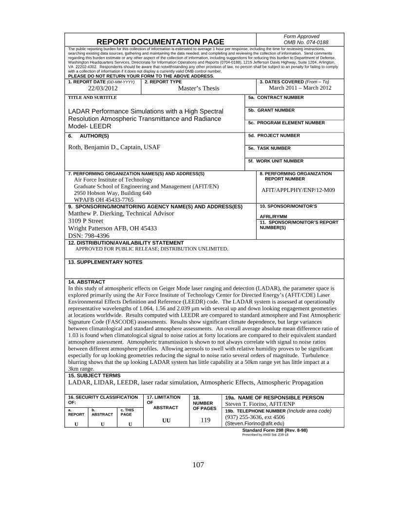
107
REPORT DOCUMENTATION PAGE Form Approved OMB No. 074-0188
The public reporting burden for this collection of information is estimated to average 1 hour per response, including the time for reviewing instructions, searching existing data sources, gathering and maintaining the data needed, and completing and reviewing the collection of information. Send comments regarding this burden estimate or any other aspect of the collection of information, including suggestions for reducing this burden to Department of Defense, Washington Headquarters Services, Directorate for Information Operations and Reports (0704-0188), 1215 Jefferson Davis Highway, Suite 1204, Arlington, VA 22202-4302. Respondents should be aware that notwithstanding any other provision of law, no person shall be subject to an penalty for failing to comply with a collection of information if it does not display a currently valid OMB control number. PLEASE DO NOT RETURN YOUR FORM TO THE ABOVE ADDRESS. 1. REPORT DATE (DD-MM-YYYY)
22/03/2012 2. REPORT TYPE
Master’s Thesis 3. DATES COVERED (From – To)
March 2011 – March 2012
TITLE AND SUBTITLE
LADAR Performance Simulations with a High Spectral Resolution Atmospheric Transmittance and Radiance Model- LEEDR
5a. CONTRACT NUMBER
5b. GRANT NUMBER
5c. PROGRAM ELEMENT NUMBER
6. AUTHOR(S)
Roth, Benjamin D., Captain, USAF
5d. PROJECT NUMBER
5e. TASK NUMBER
5f. WORK UNIT NUMBER
7. PERFORMING ORGANIZATION NAMES(S) AND ADDRESS(S) Air Force Institute of Technology Graduate School of Engineering and Management (AFIT/EN) 2950 Hobson Way, Building 640 WPAFB OH 45433-7765
8. PERFORMING ORGANIZATION REPORT NUMBER AFIT/APPLPHY/ENP/12-M09
9. SPONSORING/MONITORING AGENCY NAME(S) AND ADDRESS(ES) Matthew P. Dierking, Technical Advisor 3109 P Street Wright Patterson AFB, OH 45433 DSN: 798-4396
10. SPONSOR/MONITOR’S AFRL/RYMM 11. SPONSOR/MONITOR’S REPORT NUMBER(S)
12. DISTRIBUTION/AVAILABILITY STATEMENT APPROVED FOR PUBLIC RELEASE; DISTRIBUTION UNLIMITED.
13. SUPPLEMENTARY NOTES
14. ABSTRACT In this study of atmospheric effects on Geiger Mode laser ranging and detection (LADAR), the parameter space is explored primarily using the Air Force Institute of Technology Center for Directed Energy’s (AFIT/CDE) Laser Environmental Effects Definition and Reference (LEEDR) code. The LADAR system is assessed at operationally representative wavelengths of 1.064, 1.56 and 2.039 µm with several up and down looking engagement geometries at locations worldwide. Results computed with LEEDR are compared to standard atmosphere and Fast Atmospheric Signature Code (FASCODE) assessments. Results show significant climate dependence, but large variances between climatological and standard atmosphere assessments. An overall average absolute mean difference ratio of 1.03 is found when climatological signal to noise ratios at forty locations are compared to their equivalent standard atmosphere assessment. Atmospheric transmission is shown to not always correlate with signal to noise ratios between different atmosphere profiles. Allowing aerosols to swell with relative humidity proves to be significant especially for up looking geometries reducing the signal to noise ratio several orders of magnitude. Turbulence blurring shows that the up looking LADAR system has little capability at a 50km range yet has little impact at a 3km range. 15. SUBJECT TERMS LADAR, LIDAR, LEEDR, laser radar simulation, Atmospheric Effects, Atmospheric Propagation
16. SECURITY CLASSIFICATION OF:
17. LIMITATION OF ABSTRACT
UU
18. NUMBER OF PAGES
119
19a. NAME OF RESPONSIBLE PERSON Steven T. Fiorino, AFIT/ENP
a. REPORT
U
b. ABSTRACT
U
c. THIS PAGE
U
19b. TELEPHONE NUMBER (Include area code) (937) 255-3636, ext 4506 ([email protected])
Standard Form 298 (Rev. 8-98) Prescribed by ANSI Std. Z39-18
Top Related