


Languages
Pages
Legal


Labor Force Attachment Beyond Normal Retirement Age
Berk Yavuzoglu∗
June 1, 2015
Abstract
It is essential to understand the labor supply incentives generated by the Social Security (SS)
system to Americans beyond normal retirement age, currently 66, since the U.S. population is
growing older steadily and the �scal burden of SS is sizable. This paper analyzes the joint
determination of labor supply, consumption (savings) and the decision to apply for SS bene�ts
of elderly single males. I use a dynamic programming formulation and restricted data from the
Health and Retirement Study. I focus on the participation decision rather than the retirement
decision because a signi�cant portion of the elderly return to work after being non-participants
for a while. I account for this through wage, health status and health expenses shocks. Under-
taking a counterfactual analysis, I �nd that the year 2000 SS amendment abolishing the earnings
test for the age group 66−70 explains one-fourth of the recent increase in the elderly labor force
participation rate (LFPR). Applying the earnings test to my post-2000 sample decreases LFPR
by 2.7 percentage points and mean hours worked by 115 hours at this age group. I further �nd
via counterfactual analyses that the labor supply decision is sensitive to changes in SS bene�t
and payroll tax amounts on the extensive margin, but the e�ects on the intensive margin are not
substantial. Decreasing SS bene�ts by 20 percent increases the participation rate of the elderly
aged 66− 75 by 37 percent. Because a change in the payroll tax rate is e�ectively a change in
the wage rate, I estimate labor supply elasticities for the elderly and �nd that the elasticities
are above and around unit elasticity.
∗Department of Economics, University of Wisconsin-Madison, Madison, WI, 53705. E-mail: [email protected] am grateful to John Kennan, James Walker, Rasmus Lentz, Christopher Taber, Insan Tunali, Karl Scholz, SalvadorNavarro, Eric French, Sera�n Grundl, Francisco Franchetti and seminar participants at University of Wisconsin-Madison, University of Chicago, Paris School of Economics, Bilkent University, Sabanci University, TOBB Universityof Economics and Technology and Kazakh British Technical University for their helpful comments and suggestions.I also thank the National Bureau of Economic Research for providing me pre-doctoral fellowship through this paper.I obtained access to the Restricted Health and Retirement Survey dataset through James Walker's NICHD grant.
1

1 Motivation
The LFPR beyond normal retirement age1 was 26.2 percent for the age group 66− 69, 20.5 percent
for the age group 70 − 74, and 7.0 percent for 75+ for single males in 2006 in the U.S.2 These
levels have exhibited an upward trend since 1995 as shown in Figure 1.3 This upward trend in
the elderly participation behavior helps �nance some of the �scal burden of SS. Moreover, the U.S.
population is growing older steadily, which re�ects both aging of the baby boom generation and
increased longevity. With the increasing stock of elderly population and sizable �scal burden of SS,
it is essential to understand behavioral responses of these people to the changes in the SS system
to come up with any policy analysis.
Figure 1: Trends in Elderly Labor Force Participation Rates: Single Males
Source: Bureau of Labor Statistics
Mandatory retirement was a widespread practice in the U.S. labor market prior to the 1978
and 1986 amendments in the Age Discrimination in Employment Act.4 Since all the elderly can
decide whether to work at any age after these amendments, the recent literature treats retirement
as an individual decision. Yet, it is not obvious what the term retirement stands for. It can either
1It was 65 in 2002 and increased by 2 months each year until 2009. It is currently 66 and will be increased to 67by 2 month increments in between years 2021 and 2026.
2These statistics are enormous compared to the European countries. See Table C.1 in the Appendix. Moreover,life expectancies at age 65 are higher in most of the European countries. See Table C.2 in the Appendix.
3During that time, real value of the mean asset levels have been increasing as well except a temporary decreasein 2009. See Figure D.1 in the Appendix.
4Lazear (1979) shows that mandatory retirement can be designed as a life-cycle Pareto optimal contract solvingthe �agency problem� where workers are paid less than their value of marginal productivity when young and morewhen old.
2

mean collecting retirement bene�ts or simply quitting the labor force. Notice that retirement is
not necessarily a permanent state in the latter case since an elderly person might return to work
after being a non-participant for a while. Hence, I focus on the participation decision of individuals
beyond normal retirement age.
In this paper I analyze the labor supply, consumption and Social Security bene�ts application
decision of elderly single males jointly, using a dynamic programming formulation. The aim of the
paper is understanding the labor supply decisions of single males beyond normal retirement age
which is not well studied in the literature. I focus only on singles to avoid complexities arising
from modeling the joint decision making by couples along with shared budget constraint and leisure
complementarity.5 As a counter factual analysis, I provide an estimate of what the e�ect of the
�earnings test�6 would be on my post-2000 sample if it was not abolished by the year 2000 SS
amendment. This quanti�es the e�ect of the year 2000 SS amendment on the recent increase in
the elderly participation rates provided in Figure 1. I further decrease SS bene�t amounts by 20
percent, and estimate labor supply elasticities for the elderly to understand the e�ect of payroll
taxes on the labor supply decision since a change in the payroll tax rate is e�ectively a change in
the wage rate.7
The speci�cation of the dynamic programming model in this paper extends French (2005).
Unlike French (2005), I include three di�erent health status categories,8 health expenses, medicare,
education levels and allow limited borrowing. French (2005) shows that the �earnings test� is the
main reason for the non-participation decision of elderly people and solves the early retirement
puzzle by incorporating pension bene�ts into his model. Rust and Phelan (1997) �nd that health
care expenses and Medicare as well as SS rules are the important determinants of the retirement
decision for �nancially constrained people. Recent work by Blau and Goodstein (2010), using an
econometric model which is a linear approximation to the decision rule for employment, estimates
522.8 percent of males aged 58 − 94, the age group of interest in this paper, are single which corresponds to 9.6percent of the population. 12.1 percent of them are never married. I omit cohabiting elderly males in my study.Only 5.0 percent of single males in my sample get married within 6 years. Note that my model does not account formarriage probability. Even though the elderly single females problem resembles very much the elderly single malesproblem, I focus only on single males currently to make sure everything works well and runs smoothly for a groupconsidering the huge computational time required for estimating structural life-cycle models. Solving the model forsingle females will be relatively quick and is an extension to this paper as of now.
6See Section 6.1 for a discussion about the �earnings test.�7The change in the wage rate is determined by the economic incidence of tax. See Section 6.3 for a discussion.8French (2005) has di�culty in matching labor force participation of unhealthy individuals due to the binary
discretization of health status.
3

that 25 to 50 percent of the recent increase in elderly LFPR is attributable to the SS rules, 16 to
18 percent to increase in education and another 15 to 18 percent to increase in LFPR of married
women.9
Blau and Gilleskie (2008) investigate the e�ect of health insurance on retirement behavior.
They �nd that changes in the access to the retiree health insurance plans provided by employers or
Medicare have substantial e�ects on participation behavior for people with poor health, but only a
modest e�ect for people with good health. French and Jones (2011) have a similar context to Blau
and Gilleskie (2008), and they �nd that Medicare and employer provided health insurance, value of
which is closely tied to the health care uncertainty, are important determinants of the retirement
decision. Casanova (2010) approaches the retirement problem as a joint couple decision allowing for
leisure complementarity and shared budget constraint in a dynamic programming framework.10 She
shows that individual models of retirement decision cannot capture the incentives of couples. All the
papers mentioned above focus on the retirement decision and utilize structural models, except Blau
and Goodstein (2010). Departing from the recent literature, Maestas (2010) models participation
behavior and focuses on returning to work after being a non-participant (she calls it unretirement)
using a reduced form model. She �nds that in between 1992 and 2002, 26 percent of the elderly
unretired and 82 percent of this was anticipated.
Since the elderly population is steadily increasing and the �scal burden of SS is sizable, un-
derstanding behavioral responses of the elderly people to the changes in the SS system is essential
to come up with any policy analysis. My paper aims to accomplish this by specifying a �exible
model capturing most of the documented determinants of the elderly non-participation decision in
the literature.
9Figure D.2 in the Appendix shows that even LFPRs of singles with high school or college diploma have anincreasing pattern since 1995. Since we control for marital status and education, there should be another reasonbehind the recent increase in the elderly LFPR which Blau and Goodstein (2010) fail to explain. The reason couldbe the increase in the overall health status of the elderly.
10Casanova (2010) focuses on married people and models participation as a dichotomous decision including full-timework, part-time work and non-participation rather than a continuous hours worked decision. She further assumesthat individuals start receiving Social Security bene�ts in the �rst period they choose not to participate in the laborforce. Casanova (2010) does not account for changes in health status in her model.
4

2 Data and Preliminary Examination
Data
I use Health and Retirement Survey (HRS) data, which is a nationally representative panel data of
adults in the U.S. aged 50+, conducted biannually and �rst �elded in 1992. It contains information
on labor force participation, health, �nancial variables, family characteristics and a host of other
topics. The results in this paper are obtained using a subsample of the HRS data comprising
non-disabled single males aged 58 − 95 from 2002 to 2008. The working sample consists of 1, 691
individuals with a total of 3, 991 observations. Appendix A explains the steps used to obtain the
working sample from the raw data. I assume that attrition is missing completely at random (or
ignorable).
Preliminary Examination
This section provides a multinomial logit analysis of the labor force participation decision of single
men beyond normal retirement age. The aim is to provide basic information about the data before
executing a structural labor supply analysis of single elderly males. Since the normal retirement
age has gradually increased from 65 in 2002 to 66 in 2008 with 2 month increments, and the HRS
provides age data with 1 year increments, I consider 66 years as the cuto� age in this analysis.
LFPR of single males aged 66 to 69 is 30.4 percent, aged 70 to 74 is 23.0 percent whereas the same
statistic for single males aged 75+ is 8.2 percent in my sample. Since the unemployment rate is very
low for single males at older ages, only 0.9 percent in my sample, I do not distinguish unemployment
and out of the labor force states like Rust and Phelan (1997).
Tables 1 and 2 provide summary statistics for select variables by labor force status for age
groups 66− 74 and 75+, respectively. I de�ne part-time work as working less than 1, 600 hours in
a year.11 As seen from these Tables 1 and 2, people in the labor force are younger, more educated
and healthier on average. Full-time workers are less likely to have Medicare and more likely to have
private health insurances. There is a question in HRS inquiring about the primary health insurance
11This assumption causes me to assign elderly people who are working full-time (more than 30 hours a week) partof a year then quitting the labor force as part-time workers, which is the case for only 4.6 percent of the workersin my sample. Since this is a small statistic and the unit of time is one year in my structural model, I stick to thisde�nition.
5

Table 1: Sample Means (Standard Deviations) of Select Variables by Labor Force ParticipationStatus for Single Males Aged 66-74
Variable Full sample Full-TimeWorkers
Part-TimeWorkers
Out ofLabor Force
Age 69.985 69.064 69.876 70.159High School Dropout (reference) 0.295 0.248 0.180 0.325High School Graduate 0.508 0.516 0.444 0.519University Graduate 0.197 0.236 0.376 0.157�Fair� Health 0.333 0.217 0.247 0.368Good Health (reference) 0.324 0.306 0.337 0.325�Very Good� Health 0.343 0.478 0.416 0.307Black 0.209 0.287 0.208 0.197Medicare 0.955 0.892 0.961 0.964Has Private Insurance 0.478 0.580 0.534 0.451
Health Expenses - last 2 years1, 139.329(3, 402.939)
1, 087.637(1, 891.527)
1, 101.152(2805.693)
1, 155.108(3, 690.692)
Assets (in $1,000)325.279(657.957)
377.208(815.799)
480.299(989.001)
287.452(535.485)
# of Children2.599(2.225)
2.732(2.479)
2.404(1.738)
2.614(2.262)
Receiving Social Security 0.950 0.924 0.983 0.948Receive Pension 0.489 0.420 0.421 0.513Receive Supplement Security Income 0.045 0.000 0.011 0.058Sample size 1280 157 168 945
plan for a subset of the respondents. In my sample, 14.3 percent of respondents in the age group
66−74 who responded to this question identi�ed their primary insurance as di�erent than Medicare.
A further inspection by labor force status reveals that 47.4 percent of full-time workers, 9.7 percent
of part-time workers and 8.9 percent of non-participants have a primary health insurance di�erent
than Medicare in that age group. Notice that blacks are more likely to participate in the labor force
and part-time participants have higher asset levels. Moreover, only a small fraction of the non-
participants receive Supplemental Security Income (SSI) which implies that either their unearned
income or �nancial resources are above program limits.
To estimate a multinomial logit model of labor force status, consider the latent utility model:
y∗ij = θ′ijzi + ηij for j = 1, 2, 3. (1)
where i denotes individuals, y∗ij 's denote the unobserved utilities obtained from the choice of labor
6

Table 2: Sample Means (Standard Deviations) of Select Variables by Labor Force ParticipationStatus for Single Males Aged 75+
Variable Full sample Full-TimeWorkers
Part-TimeWorkers
Out ofLabor Force
Age 82.814 79.320 79.981 83.080High School Dropout (reference) 0.407 0.340 0.302 0.415High School Graduate 0.440 0.420 0.406 0.442University Graduate 0.154 0.240 0.292 0.143�Fair� Health 0.405 0.200 0.226 0.421Good Health (reference) 0.318 0.460 0.406 0.309�Very Good� Health 0.278 0.340 0.368 0.270Black 0.145 0.120 0.113 0.148Medicare 0.973 0.980 0.972 0.973Has Private Health Insurance 0.552 0.700 0.538 0.548
Health Expenses - last 2 years2, 042.713(8, 024.231)
1, 328.160(2, 611.560)
1, 145.613(1, 773.819)
2, 116.125(8, 341.904)
Assets (in $1,000)353.765(856.189)
765.263(1, 359.691)
798.521(1, 919.149)
315.763(715.047)
# of Children3.024(2.287)
2.940(2.385)
3.104(2.212)
3.021(2.290)
Receiving Social Security 0.970 0.980 0.981 0.969Receive Pension 0.577 0.300 0.349 0.598Receive Supplemental Security Income 0.031 0.020 0.000 0.033Sample size 1, 938 50 106 1, 782
force participation status j, zi is the vector of explanatory variables given in Tables 1 and 2 excluding
endogenous variables, θij 's are the corresponding vectors of unknown coe�cients and ηij 's are the
random disturbances.
Let r = max (y∗1, y∗2, y
∗3, ). Then, the labor status is given by
lfp =
1 = full-time, if r = y∗1,
2 = part-time, if r = y∗2,
3 = out of labor force, if r = y∗3,
(2)
I assume that ηj 's satisfy the Independence of Irrelevant Alternatives (IIA) hypothesis, so they
have type I extreme value distribution. McFadden (1974) proves that this speci�cation corresponds
to the Multinomial Logit model.
7

Table 3: Multinomial Logit Estimates of Labor Force Status on Some Possible Determinants forSingle Males Aged 66-74
Variable Full-Time Part-TimeCoef. Std. Err. Coef. Std. Err.
Age −0.159∗∗∗ 0.035 −0.033 0.034High School Graduate 0.192 0.219 0.435∗ 0.236University Graduate 0.550∗∗ 0.265 1.514∗∗∗ 0.268�Fair� Health −0.394∗ 0.242 −0.342 0.216Very Good Health 0.439∗∗ 0.206 0.090 0.203Black 0.674∗∗∗ 0.205 0.308 0.216Health Expenses (in $1000) 0.003 0.019 −0.011 0.025Has Children −0.066 0.204 0.368∗ 0.204Constant 8.865∗∗∗ 2.419 −0.219 2.417
No. of observations 1, 280Log-likelihood w/o covariates −967.3Log-likelihood with covariates −916.2
Robust standard errors are in parentheses.
* signi�cant at 10%; ** signi�cant at 5%; *** signi�cant at 1%.Good health is the reference group for health status. High school dropouts is the reference group for education.
The choice probabilities are given by
πj = Pr(lfp = j | z) =exp(θ
′jz)
3∑k=1
exp(θ′kz)
, j = 1, 2, 3. (3)
Since3∑l=1
πl = 1, I choose people who are out of the labor force as the reference group and set
θ3 = 0. Then, I obtain consistent estimates for θj 's by maximizing the following likelihood function
L =∏lfp=1
π1∏lfp=2
π2∏lfp=3
π3. (4)
The results of this estimation can be found in Table 3 for the age group 66− 74.12 Notice that
the log odds of staying in the labor force decrease with age and increase with education level and
health stock. The results also suggest that being black increases full-time participation probability
while having children increases part-time participation probability for which I do not have a good
explanation.
12Multinominal logit estimates for the age group 75+ can be found in Table C.3 in the Appendix.
8

3 Model
I use a dynamic programming formulation. I have a three dimensional vector of control variables:
consumption, hours worked in a year and a dummy variable indicating whether the individual
applied for SS bene�ts. Consumption (ct) and hours worked (ht) are continuous variables obtained
via splines after using discretizations.13 bt denotes the dummy variable indicating whether the
individual applied for SS bene�t or not.
The observed heterogeneity comes from a �ve dimensional vector of state variables: assets,
wages, health status, education and Principal Insurance Amount (PIA), the term which gives the
basis for SS bene�t amounts. I use 11 asset states denoted by At, 6 wage states denoted by wt and
5 PIA states.14 There are 4 health status categories: �very good,� good, �fair� and dead15 denoted
by hst taking values 1, 2, 3 and 4, respectively. I have 3 education (edt) groups: no high school
diploma (ed < 12 years of education), high school graduates (12 ≤ ed < 16 years of education) and
university graduates (ed ≥ 16 years of education).16 I use a projection method to accommodate
continuous state space of assets, wages and PIA. I control for Medicare (mt) in my model, and
include SS bene�ts (sst) and Medicare premium (mp) in the budget constraint.
The subjects make decisions every year in my model. Denote the control variables by d, state
variables by x, and preference parameters by θ. The �ow utility function, for each health status
category iε {very good health, good health and fair health}, is given by:
U(xt, dt, θ) =1
1− v
(cθCit LθLi
)1−v(5)
where
L = L−(ht+θP,f +θP,goodI(good health)+θP,fairI(fair health)+θPA(aget−57)γ)I(ht > 0), (6)
13The initial discretization used for consumption is 3, 000, 13, 000, 23, 000, 33, 000, 53, 000, 73, 000, 93, 000, 113, 000,143, 000, 173, 000 and 203, 000. The initial discretization used for hours worked is 0, 750, 1500, 2250, 3000 and 3750.
14The initial asset states are given by −15, 000, 0, 15, 000, 40, 000, 80, 000, 120, 000, 200, 000, 300, 000, 500, 000,800, 000 and 1, 300, 000. The initial wage states are given by 2, 8, 14, 20, 32 and 44. The initial PIA states are 0,25thpercentile, 50thpercentile, 75thpercentile and the maximum observed amount.
15HRS has 5 self-reported health status categories: excellent, very good, good, fair and poor. I combine the self-reported excellent and very good health status categories and call the new category as �very good,� and combine fairand poor health status categories and call the new category as �fair.�
16My sample is not big enough to conduct separate analyses by education groups.
9

The coe�cient of relative risk aversion is given by v. For each health status category i, θCi and
θLi measure the consumption and leisure weights, respectively. I(.) is the indicator function. θPf
is the �xed cost of work, and θP,good and θP,fair are the additional participation costs depending on
health status level, with θP,very good normalized to zero. θPA(aget−57)γ measures the participation
cost explained by age.
Following De Nardi (2004), people who die value asset bequests according to the function
b(At) = θB(At +K)θC2(1−v)
1− v(7)
where K measures the curvature of the function. With K > 0, the disutility of leaving non-positive
bequests in the amount of less than K dollars becomes �nite. The curvature implicitly sets a
borrowing constraint since the elderly face mortality uncertainty each period.
The constraints are the wage determination equation, the health status determination equation,
the health expenses determination equation and the asset accumulation equation.
I do not observe wages for more than half of the employed workers. I impute them using the
solution methodology for double selection problems provided by Tunali and Yavuzoglu (2012), which
relaxes the trivariate normality assumption among the error terms of the two selection equations
and the regression equation by following the Edgeworth expansion approach of Lee (1982). The
details can be found in Appendix B.
Log wages in the current period depend on age, education and PIA:17
ln(wt) = ς0 + ς1aget + ς2aget
2
100+ δhighI(12 ≤ edt < 16) + δuniI(edt ≥ 16) + δPIA
PIA
100+ARt, (8)
where
ARt = ρARARt−1 + ηt, ηt ∝ N(0, σ2η). (9)
According to the human capital theory, workers should be paid their marginal product which de-
creases over the time due to the decrease in health stock and human capital investment. The
resulting wage process is approximated through Equations 8 and 9. PIA is included as a proxy for
work experience since it is calculated averaging the 35 highest earnings years, and zeros are thrown
17Having no high school diploma is the reference category for high school and university graduates.
10

into the calculation in case an elderly person has a working history of less than 35 years.18
Health status next period (including being dead) depends on the current health status, age and
education:19
µj,i,aget,ed = Pr(hst+1 = j|hst = i, aget, ed). (10)
Out of pocket health expenses depend on age, health status, medicare and asset levels:20
ln(het) = ϕ0 + ϕ1aget +ϕ2
100aget
2 + δfairI(fair health) + δgoodI(good health)
+ δmedicaremt + δassets
(At
100, 000
)+ ξt, (11)
where
ξt ∝ N(0, σ2ξ ). (12)
The age dependency of out of pocket health expenses arises from the increasing hazard rates of
serious illnesses with age. I assume everyone is entitled to Medicare at age 65, which causes a
reduction in out-of-pocket health expenses. This, in turn, provides an incentive for the elderly to
leave the labor force. I include asset levels in Equation 11 because of the positive correlation between
wealth and the quality of care demanded. Moreover, poor people might be covered by Medicaid
when confronted with high out-of-pocket health expenses.21
The asset accumulation equation is given by:
At+1 = (1 + r)At + Y1(wtht, τ1) + btsst − het − ct −mp− Y2(Gt, τ2), (13)
where r is the interest rate, Y1(wtht, τ1) is the level of post-FICA tax wage earnings, τ2 is the tax
structure regarding state and federal taxes and Y2(Gt, τ2) is the level of tax amount paid out of
gross taxable earnings, Gt. It is generated via:
18See Section 4.3 for a discussion about the relationship between Average Indexed Monthly Earnings (AIME) andPIA.
19See Section 4.1 for the functional form.20�Very good� health status is the reference category for good and �fair� health statuses.21The magnitude of the standard deviation of the out of pocket health expenses corresponds to the 97.6th percentile
of the distribution in my sample. Most elderly would not face extreme out-of-pocket expenses amounts or uncertainty(standard deviation) unless they choose to have exceptional care. For that reason, I use out-of-pocket health expensesvalues up to the 96thpercentile of the distribution to calculate the data moments required for estimation.
11
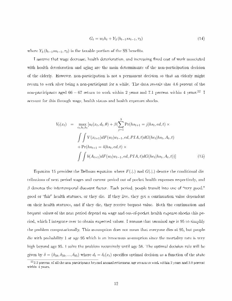
Gt = wtht + Y3 (bt−1sst−1, τ3) (14)
where Y3 (bt−1sst−1, τ3) is the taxable portion of the SS bene�ts.
I assume that wage decrease, health deterioration, and increasing �xed cost of work associated
with health deterioration and aging are the main determinants of the non-participation decision
of the elderly. However, non-participation is not a permanent decision so that an elderly might
return to work after being a non-participant for a while. The data reveals that 4.6 percent of the
non-participants aged 66 − 67 return to work within 2 years and 7.1 percent within 4 years.22 I
account for this through wage, health status and health expenses shocks.
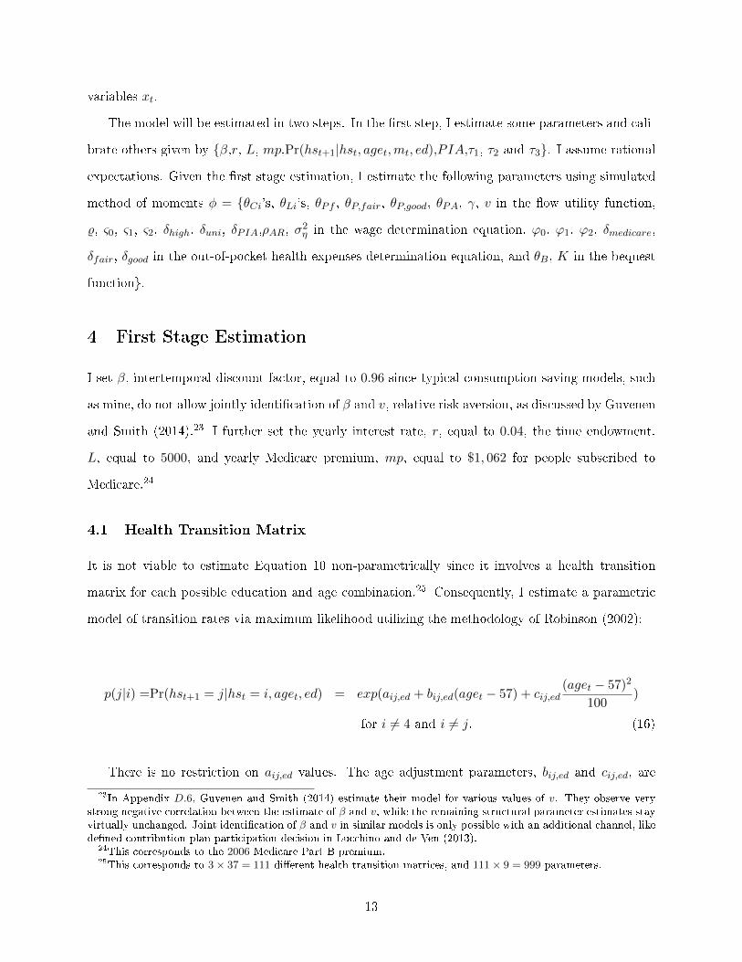
Vt(xt) = maxct,bt,ht
[ut(xt, dt, θ) + β(3∑j=1
Pr(hst+1 = j|hst, ed, t)×
ˆ ˆV (xt+1)dF (wt|wt−1, ed, PIA, t)dG(het|hst, At, t)
+Pr(hst+1 = 4|hst, ed, t)׈ ˆb(At+1)dF (wt|wt−1, ed, PIA, t)dG(het|hst, At, t))] (15)
Equation 15 provides the Bellman equation where F (.|.) and G(.|.) denote the conditional dis-
tributions of next period wages and current period out-of-pocket health expenses respectively, and
β denotes the intertemporal discount factor. Each period, people transit into one of �very good,�
good or �fair� health statuses, or they die. If they live, they get a continuation value dependent
on their health statuses, and if they die, they receive bequest value. Both the continuation and
bequest values of the next period depend on wage and out-of-pocket health expense shocks this pe-
riod, which I integrate over to obtain expected values. I assume that terminal age is 95 to simplify
the problem computationally. This assumption does not mean that everyone dies at 95, but people
die with probability 1 at age 95 which is an innocuous assumption since the mortality rate is very
high beyond age 95. I solve the problem recursively until age 58. The optimal decision rule will be
given by δ = (δ58, δ59, ..., δ95) where dt = δt(xt) speci�es optimal decision as a function of the state
222.2 percent of all the non-participants beyond normal retirement age return to work within 2 years and 3.0 percentwithin 4 years.
12
variables xt.
The model will be estimated in two steps. In the �rst step, I estimate some parameters and cali-
brate others given by {β,r, L, mp,Pr(hst+1|hst, aget,mt, ed),P IA,τ1, τ2 and τ3}. I assume rational
expectations. Given the �rst stage estimation, I estimate the following parameters using simulated
method of moments φ = {θCi's, θLi's, θPf , θP,fair, θP,good, θPA, γ, v in the �ow utility function,
%, ς0, ς1, ς2, δhigh, δuni, δPIA,ρAR, σ2η in the wage determination equation, ϕ0, ϕ1, ϕ2, δmedicare,
δfair, δgood in the out-of-pocket health expenses determination equation, and θB, K in the bequest
function}.
4 First Stage Estimation
I set β, intertemporal discount factor, equal to 0.96 since typical consumption-saving models, such
as mine, do not allow jointly identi�cation of β and v, relative risk aversion, as discussed by Guvenen
and Smith (2014).23 I further set the yearly interest rate, r, equal to 0.04, the time endowment,
L, equal to 5000, and yearly Medicare premium, mp, equal to $1, 062 for people subscribed to
Medicare.24
4.1 Health Transition Matrix
It is not viable to estimate Equation 10 non-parametrically since it involves a health transition
matrix for each possible education and age combination.25 Consequently, I estimate a parametric
model of transition rates via maximum likelihood utilizing the methodology of Robinson (2002):
p(j|i) =Pr(hst+1 = j|hst = i, aget, ed) = exp(aij,ed + bij,ed(aget − 57) + cij,ed(aget − 57)2
100)
for i 6= 4 and i 6= j. (16)
There is no restriction on aij,ed values. The age adjustment parameters, bij,ed and cij,ed, are
23In Appendix D.6, Guvenen and Smith (2014) estimate their model for various values of v. They observe verystrong negative correlation between the estimate of β and v, while the remaining structural parameter estimates stayvirtually unchanged. Joint identi�cation of β and v in similar models is only possible with an additional channel, likede�ned contribution plan participation decision in Lucchino and de Ven (2013).
24This corresponds to the 2006 Medicare Part B premium.25This corresponds to 3× 37 = 111 di�erent health transition matrices, and 111× 9 = 999 parameters.
13

Table 4: Maximum Likelihood Estimates of the Health Status Determination Equation for MaleHigh School Graduates
aij,ed=high−schooli � j �very good� good �fair� dead
�very good� − −1.970(0.052)
−3.814(0.147)
−5.661(0.225)
good−1.588(0.108)
− −2.113(0.064)
−4.996(0.195)
�fair�−2.996(0.207)
−1.539(0.124)
− −4.066(0.204)
bij,ed=high−school cij,ed=high−school
i < j (recovery)−0.033(0.015)
0.064(0.048)
j = 4 (death)0.078(0.016)
0.024(0.036)
i > j (deterioration)0.001(0.001)
0.071(0.013)
restricted to 3 values: one for recovery (i < j), one for mortality (j = 4) and one for health
deterioration (i > j). The parameters estimates for high school graduates can be found in Table
4.26 Notice that the higher the estimate is (in absolute value) the lower the probability.
To assess the performance of the estimation, I compare the implied 2 year transition rates in the
model with the data at the �rst quartile, median and third quartile of the age distribution, provided
in Table 5. The model �t looks reasonable.
Table 5: Observed and Fitted Biannual Health Status Transition Matrices for Male High SchoolGraduates
Observed Frequencies Fitted Frequencies
Around the First Age Quartile (63− 65) A the First Age Quartile (= 64)
i � j �very good� good �fair� dead �very good� good �fair� dead�very good� 70.4% 23.4% 4.4% 1.7% 70.6% 22.6% 5.5% 1.4%
good 24.2% 54.4% 19.3% 2.1% 25.7% 52.9% 18.7% 2.6%�fair� 9.4% 25.9% 57.4% 7.4% 9.3% 25.8% 59.1% 5.7%
Around the Median Age (68− 70) At the Median Age (= 69)
�very good� 66.1% 24.6% 7.9% 1.4% 68.0% 24.2% 6.1% 2.1%good 22.1% 55.7% 18.5% 3.6% 23.1% 52.9% 20.3% 3.9%�fair� 7.8% 20.0% 65.1% 7.2% 8.1% 23.5% 59.9% 8.6%Around the Third Age Quartile (75− 77) At the Third Age Quartile (= 76)
�very good� 61.9% 26.6% 6.8% 4.7% 62.0% 27.3% 7.5% 4.0%good 21.8% 51.2% 21.4% 5.6% 20.3% 49.8% 23.2% 7.3%�fair� 6.1% 24.8% 54.7% 14.4% 7.1% 21.0% 57.2% 15.4%
26I provide the estimates for high school dropouts and university graduates in Tables C.4-C.7 in the Appendix.The implied biannual transition rates from the model are utilized to get the maximum likelihood estimates.
14

4.2 Taxes
FICA is a federal payroll tax imposed on workers. It has two components: Social Security tax
and Medicare tax. During the period 1990-2010, the Social Security tax rate was 6.2 percent of an
employee's wages up to a threshold of earnings known as the Social Security Wage Base,27 and the
Medicare tax rate was 1.45 percent of an employee's wages without any cap. I use these values to
set τ1.
The second portion of the tax structure, τ2, includes federal and state income tax rates. I
take the federal income tax rates from the 2006 annual tax rate schedules accounting for standard
deductions by age and personal exemptions which phase out after an income threshold. As state
income taxes, I use the 2006 Rhode Island tax rate schedule following French and Jones (2011).28
The current regulation for federal income taxation of SS bene�ts is determined by The De�cit
Reduction Act of 1993. For a single elderly individual, up to 50% of the SS bene�ts are subject to
taxation if his combined income (the sum of adjusted gross income plus nontaxable interest plus
one-half of SS bene�ts) is between $25, 000 and $34, 000. If his combined income is more than
$34, 000, up to 85 percent of his SS bene�ts are taxable. I generate the precise taxable income using
IRS Publication Number 915 to set τ3. In doing this I omit nontaxable interest since I do not have
a measure of it.
4.3 Social Security Bene�t Levels
Social Security bene�t levels are calculated using Average Indexed Monthly Earnings (AIME), which
is the average of 35 highest indexed earnings years.29 Then, a formula is applied on AIME to compute
Primary Insurance Amount (PIA) which gives the basis for SS bene�t level.
I obtain the AIME levels for 72.1 percent of respondents exploiting their work history from the
restricted data set using 2006 as index year. I observe the SS bene�t amount of another 20.8 percent
of the sample even though I cannot see their full work history. I generate AIME values for this
27In the time period under study, Social Security Wage Base increased from $84, 900 to $102, 000. For simplicity,I �x the Social Security Wage Base at the year 2006 value, $94, 200, in my analysis.
28The taxation of self-employed workers, 30 percent of workers in my sample, is very similar to that of employees.This is why I do not control for taxation of self-employed seperately.
29For AIME calculation, earnings levels in any year cannot exceed the maximum taxable earnings level of that yeardetermined by the Social Security Administration. The index used for AIME is called the �national average wageindex�.
15

subsample through an inverse function of the bene�t levels.30 I impute the AIME values for the
rest of the sample. PIA is given by 90 percent of the �rst $656 of AIME plus 32 percent of AIME
over $656 and through $3, 955, plus 15 percent of AIME over $3, 955.
I assume that AIME values are constant, so working another year does not have any e�ect on
that value. For people having at least 35 years of work history, the incremental increase in AIME
level is either zero (if the earnings in the extra year does not exceed 35th highest earning year)
or close to zero. Moreover, at least 10 years of working history are required to be entitled to SS
bene�ts. Only 9.4 percent of workers in my sample have 5 to 34 years or working history.
5 Results
5.1 Solution Methodology
I employ the simulated method of moments strategy where I match the following moments:
• By age, participation rate for the age group 60− 85 and mean hours worked for participants
for the age group 60− 72 to identify θC,i and θL,i for each health status i, θP,A, γ, and v.
• For each health status, average of participation rates between ages 66 − 74 to identify θP,f ,
θP,good and θP,fair.
• By age, mean wage for the age group 60− 75 to identify ς0, ς1 and ς2.
• For each education level, average of mean wages between ages 61 − 70 to identify δhigh and
δuni.
• For three PIA intervals, average of mean wages between ages 62− 67 to identify δPIA .
• Covariance of wages between ages 65 and 67 for participants to identify ρAR.
• Average of standard deviation of wages between ages 62− 67 to identify σ2η.
• By health status, mean out-of-pocket health expenses for age groups ages 68−69 and 78−79.
This helps me identify γ0, γ1, γ2, δgood and δfair.
30In doing so, I increase SS bene�t amount of early retirees by 25 percent which is equivalent to assuming thatthey retired 36 months earlier than their full retirement age. I index the bene�t amounts according to the 2006 level.I also consider Medicare premiums deducted from SS bene�t check while calculating AIME levels.
16

• Mean out-of-pocket health expenses for age groups 61− 63 and 68− 70 to identify δmedicare.
• Mean out-of-pocket health expenses for age group 67−75 by assets levels 0−40, 000, 40, 000−
200, 000 and 200, 000− 1, 000, 000 to identify δassets.
• Average of standard deviation of out-of-pocket health expenses between ages 62−67 to identify
σ2ξ .
I assume that at the terminal age agents are non-participants and consume all of their assets. In
solving the model, I calculate the expectations of value and bequest functions using the Gauss-
Hermite quadratures of order 5 to account for the wage and health expense shocks. The next step
is to randomly draw 1, 000 observations from the data using the Mersenne Twister random number
generator and simulate their behavior with interpolation/extrapolation. Subsequently, the distance
between the simulated and the data moments are computed. In doing this, I use the the inverse of the
variance covariance matrix of the data moments as the weight matrix to obtain e�cient estimates.31
This process is repeated with di�erent parameter vector choices using the Nelder-Mead algorithm.
The solution is given by the parameters minimizing the distance between the simulated and the
true data moments.
5.2 Parameter Estimates
The estimates are provided in Table 6. While consumption share parameters are positively asso-
ciated with health status, the leisure share parameters are negatively correlated except very good
health. Given the same age and PIA levels, compared to people having no high school diploma, high
school graduates earn 11 percent more on average while college graduates earn 37 percent more.
The part of wages unexplained by the observables shows 72 percent persistency over a year.
Given the same age and asset levels, the elderly with good health pay 7 percent less out-of-pocket
health expenses than ones with �very good� health whereas the elderly with �fair� health pay 15
percent more on average. Having Medicare decreases out-of-pocket health expenses by 54 percent.
Given the same age level and health status, an increase of $100, 000 in asset levels are associated
with a 4 percent increase in out-of health expenses on average.
31The variance covariance matrix of data moments is estimated via bootstrap using 1, 000 replications.
17

Table 6: The Estimates of the Structural Parameters
Parameter Explanation Coef. Std. Error Parameter Explanation Coef. Std. Error
Flow Utility Parameters Wage Equation Parameters
θC,verygood Cons. weight, �very good� health 0.486 0.010 ς0 Constant 1.078 0.020θC,good Cons. weight, good health 0.454 0.008 ς1 Age 0.066 0.001θC,fair Cons. weight, �fair� health 0.453 0.012 ς2 Age squared/100 −0.075 0.001
θL,verygood Leisure weight, �very good� health 0.570 0.013 δhigh school High school wage premium 0.105 0.014θL,good Leisure weight, good health 0.506 0.015 δuniversity University wage premium 0.374 0.029θL,fair Leisure weight, �fair� health 0.518 0.019 δPIA PIA/100 (proxy for experience) 0.008 0.000θPf Fixed cost of work (hours worked) 889.0 5.6 ρAR AR term 0.715 0.046θP,good Add. part. cost - good health 493.0 0.3 σ2η Variance of the error 0.060 0.004
θP,fair Add. part. cost -�fair� health 1572.0 30.6 Health Expenses Equation Parameters
θPA Participation Cost due Age - Shifter 1.576 13.7 γ0 Constant 4.084 0.055γ Participation Cost due Age - Convexity 2.045 0.021 γ1 Age 0.015 0.0001v Relative risk aversion 4.144 0.136 γ2 Age squared/100 0.0007 0.0002
δgood Premium for good health −0.073 0.006δfair Premium for �fair� health 0.153 0.023
Bequest Function Parameters δmedicare Premium for Medicare −0.544 0.002θB Bequest Shifter 0.00008 0.000001 δassets Premium for Assets ($100,000) 0.044 0.007K Curvature 11, 850 42 σ2ξ Variance of the error 1.930 0.016
Notes: Bootstrapped standard errors (using 100 replications) are reported.
No high school diploma is the reference category for wage premium parameters.�Very good� health is the reference category for health expenses premium coe�cients.
The curvature estimate implies that the elderly can have unsecured debt up to $11, 850,32 which
can be thought of maxing out credit cards rather than borrowing against SS bene�ts. Figure 2
provides the participation cost due to age.
Figure 2: Participation Cost Explained by Age
32The elderly can have more debts as long as they have corresponding assets for these debts like mortgage. Thebequest function implies having an asset level less than −$5, 320 produces in�nite disutility. The data suggest thatsome elderly people do borrow small amounts of money. While 3.6 percent of the elderly have negative assets levelsin the data, only 1.8 percent have asset levels less than −$5, 320.
18

5.3 Model Fit
Figures 3, 4 and 5 provides the model �t of participation rate, mean hours worked and mean wages
for participants, respectively. Simulated pro�les provides the path of average behavior here and
elsewehere in the paper. Table 7 provides the model �t of the average of mean wages between ages
61 and 70 by education group. Table 8 shows the model �t of the average of mean wages between
ages 62 and 67 by three PIA intervals. Table 9 provides the model �t of the average of participation
rates between ages 66 and 74 by health status. Table 10 provides the model �t of the average of
mean health expenses between ages 67− 70 and 71− 74 by health status. Table 11 shows model �t
of the average health expenses between ages 67 − 75 by asset levels. Table 12 provides the model
�t of the remaining moments. The model �ts the data well with reasonable estimates.
Figure 3: Model Fit - Participation Rate by Age
Figure 4: Model Fit - Mean Hours Worked for Participants by Age
19

Figure 5: Model Fit - Mean Wages for Participants by Age
Table 7: Model Fit - Average of Mean Wages of Each Age between 61− 70 by EducationEducation Status Data Simulation
No High School Diploma 10.74 10.46
High School Graduates 12.86 12.14
University Graduates 16.60 15.35
Table 8: Model Fit - Average of Mean Wages between Ages 62 and 67 by PIAPIA Level Data Simulation
PIA < 1, 000 12.78 11.06
1, 000 <PIA < 1, 500 13.33 13.35
PIA > 1, 500 15.18 14.15
Table 9: Model Fit - Average of Participation Rates between Ages 66 and 74 by Health StatusHealth Status Data Simulation
�Very Good� 0.337 0.326
�Good� 0.262 0.226
�Fair� 0.193 0.165
Table 10: Average of Mean Health Expenses between Ages 67− 70 and 71− 74 by Health StatusAges 68− 69 Ages 78− 79
Health Status Data Simulation Data Simulation
�Very Good� 628 589 653 707
�Good� 739 776 714 640
�Fair� 735 783 798 786
20

Table 11: Average Health Expenses between Ages 67− 75 by AssetsAssets Data Simulation
0− 40, 000 495 595
40, 000− 200, 000 747 607
200, 000− 1, 000, 000 841 719
Table 12: Model Fit - RestData Simulation
Covariance of Wages Between Ages 65 and 67 (For Participants in Both Periods) 12.72 18.51
Average of Standard Deviation of Wages Between Ages 62 and 67 5.18 5.02
Average of Health Expenses Between Ages 61− 63 784 803
Average of Health Expenses Between Ages 68− 70 708 708
Average of Standard Deviation of Health Expenses Between Ages 62 and 67 1, 233 1, 236
6 Counterfactuals
6.1 The E�ect of Year 2000 Social Security Amendments
�Earning test� is a program deferring part (or all) of SS bene�ts of people whose earnings exceed a
threshold level to later years by indexing the withheld amount with the delayed retirement credit.
Until year 2000, it applied to the elderly until the age 70, and it currently applies only on the elderly
who start collecting their SS bene�ts before normal retirement age. The annual delayed retirement
credit was 3.0 percent in 1989 and was raised by 0.5 percentage point every two years since then
until 2008. That corresponded to 5.5 percent delayed retirement credit right before the year 2000
SS amendment, which was actuarially unfair. It is 8 percent now and can be considered actuarially
fair.33 �Earnings test� withholds $1 in bene�ts for every $2 of earnings in excess of the lower exempt
amount, and $1 in bene�ts for every $3 of earnings in excess of the higher exempt amount. The
lower and higher exempt amount are determined by the Social Security Administration.
The time period studied in the paper is 2002− 2008, right after the abolishment of the earnings
test. It is possible to see the behavioral e�ects of the year 2000 SS amendment by applying the
pre-2000 rules on my sample. I set the delayed retirement credit to 4.5 percent and use 2006 values
33Assume that the yearly retirement bene�ts of a SS bene�ciary is equal to $10, 000. The CDC report in 2009indicates that the life expectancy at age 65 was around 19 years. Since the SS makes the yearly cost-of-livingadjustment on the retirement bene�ts, I assume that the real value of the bene�ts stays the same. If this bene�ciarydelays getting retirement for a year, he gets $10, 800 for 18 years on average, and if he does not delay the retirement,he gets $10, 000 for 19 years on average. Note that 10, 800 ∗ 18 w 10, 000 ∗ 19.
21

Figure 6: The E�ect of Earnings Test-Extensive Margin
of lower and higher exempt amounts rather than 2000 values.
Figure 6 shows that LFPR of the elderly aged 66− 70 decreases by 2.7 percentage points with
the �earnings test� explains one-fourth of the recent increase in the elderly participation rates. The
e�ect on the intensive margin is substantial as well and provided in Figure 7. Notice mean annual
hours worked decreases by 115 hours in the same age group. The mean earnings of participants at
age 66 with the introduction of earnings test, $13, 680, gets very close to the lower exempt amount
of earnings test, $12, 480. This suggests that the elderly limited their hours supplied to avoid the
implicit taxation imposed by the earnings test.
Figure 7: The E�ect of The Earnings Test - Intensive Margin
6.2 Changing Social Security Bene�t Amounts
In my second counterfactual analysis, I decrease SS bene�t amounts by 20 percent. This is mainly
an income e�ect for the elderly with a small substitution e�ect arising from a possible change in
22

Figure 8: Participation Rates under 20% Decreased SS Bene�t Levels
the decision to start collecting retirement bene�ts. The participation decision is sensitive to Social
Security bene�ts as seen in Figure 8. 20 percent decrease in SS bene�ts is associated with a 37
percent increase in LFPR of the age group 66 − 75.34 However, there is not a signi�cant response
in the intensive margin as presented in Figure 9.
Figure 9: Mean Hours Worked under 20% Decreased SS Bene�t Levels
6.3 Labor Supply Elasticities and Changes in Payroll Taxes
In my last analysis, I examine the e�ect of a change in payroll taxes on the elderly labor supply
decisions. Notice that a change in the payroll tax rate is e�ectively a change in the wage rage.
34For those who �nd 20 percent decrease in SS bene�ts politically unacceptable, 10 and 5 percent decrease causeparticipation rate to increase by 16 and 8 percent, respectively. The resulting simulated pro�les for these two casesare in between the baseline and 20 percent decrease pro�les.
23

The corresponding change in the wage rate is determined by the economic incidence of tax. Joint
Committee on Taxation (2001) postulates that the incidence of the federal payroll taxes falls entirely
on employees. Li (2015) �nds that workers bear the full burden of the federal payroll tax in the U.S.
using a di�erence-in-di�erence approach. Exploiting the year 1981 amendment in payroll taxation
in Chile, Gruber (1997) obtains the same result. I conduct my analysis here assuming that the
incidence is passed entirely to the workers following Li (2015) and Gruber (1997).
I decrease FICA tax amounts by 25 for everyone starting at the age 58, the initial age in my
dynamic programming set-up. This can be thought of as a 3.825 percent increase in wages as well.
This kind of analysis will have both income and substitution e�ects on the elderly. Figure 10 shows
that such a policy change a�ects the extensive margin mainly beyond normal retirement age. The
corresponding increase in the LFPR for people aged 66− 70 is 6.6 percent, which corresponds to a
labor supply elasticity of 1.73.
Figure 10: Participation Rates under Decreased FICA Amounts for Everyone
Figure 11 provides the labor supply responses to decreased FICA levels on the intensive margin.
The e�ects are not substantial. The elderly increase their annual hours supplied by an average of
25 hours on average between ages 61− 65, but decrease it by an average of 50 hours at ages 66 and
67.
If FICA taxes are reduced only for people aged 70+, the response in the extensive margin is
observed mainly between ages 70 and 73. The corresponding increase in LFPR is 3.8 percent on
these age groups, which corresponds to unit labor supply elasticity. The e�ect on the intensive
margin is not substantial again.
24

Figure 11: Mean Hours Worked under Decreased FICA Amounts for Everyone
Figure 12: Participation Rates under Decreased FICA Amounts for People Aged 70+
Figure 13: Mean Hours Worked under Decreased FICA Amounts for People Aged 70+
25

7 Conclusion
This paper analyzes the joint determination of labor supply, consumption and the decision to apply
for SS bene�ts of elderly single males using a dynamic programming formulation and restricted data
from the HRS. I �rst conduct a preliminary multinomial logit analysiss, then formulate a dynamic
programming model enhancing the understanding of the elderly labor force decision. In doing so, I
focus on the participation decision rather than the retirement decision since a signi�cant portion of
the elderly return to work after being non-participants for a while.
The speci�cation of my model is �exible in terms of capturing most of the documented determi-
nants of the elderly non-participation decision in the literature. I apply �earnings test,� which was
abolished by the year 2000 SS amendment, on my sample via a counter-factual analysis to quantify
the e�ect of the year 2000 SS amendment on the recent increase in the elderly participation rates. I
�nd that the abolishment of the �earnings test� increased the participation rate of the elderly single
males aged 66−70 by 2.7 percentage points on the extensive margin and mean annual hours worked
by 115 hours on the intensive margin. The e�ect on the extensive margin explains one-fourth of the
recent increase in the elderly participation rates. Moreover, the decrease in the intensive margin
brings the mean earnings level very close to the lower exempt amount of �earnings test.� This �nd-
ing suggests that prior to the year 2000 SS amendment, the elderly limited their hours supplied to
avoid the implicit taxation imposed by the �earnings test� via an unfair delayed retirement credit.
In my other counterfactual analyses, I consider some changes in SS rules. I �nd that decreasing
SS bene�ts by 20 percent increases the participation rate of the elderly single males aged 66 − 75
by 37 percent without a substantial e�ect on the intensive margin. The e�ect of changing FICA
taxes can be found by estimating labor supply elasticities since a change in the payroll tax rate is
e�ectively a change in the wage rate and workers bear the full burden of FICA in the U.S. I �nd
that labor supply elasticities for the elderly are above and around unit elasticity. The e�ect on the
intensive margin is not substantial again. It is essential to understand the incentives provided by
the SS system on the elderly labor supply decision since the U.S. population is steadily aging and
the �scal burden of SS is sizable. These results suggest that the policy recommendations arising
within the public debate to change the SS rules might have a marked e�ect on the participation
decision of people beyond normal retirement age.
26

References
Blau, D. M. and D. B. Gilleskie (2008): �The Role of Retiree Health Insurance in the Employ-
ment Behavior of Older Men,� International Economic Review, 49, 475�514.
Blau, D. M. and R. M. Goodstein (2010): �Can Social Security Explain Trends in Labor Force
Participation of Older Men in the United States?� Journal of Human Resources, 45, 328�363.
Casanova, M. (2010): �Happy Together: A Structural Model of Couples' Joint Retirement
Choices,� Working paper.
De Nardi, M. (2004): �Wealth Inequality and Intergenerational Links,� The Review of Economic
Studies, 71, 743�768.
French, E. (2005): �The E�ects of Health, Wealth and Wages on Labor Supply and Retirement
Behavior,� Review of Economic Studies, 72, 395�427.
French, E. and J. B. Jones (2011): �The E�ects of Health Insurance and Self-Insurance on
Retirement Behavior,� Econometrica, 79, 693�732.
Gruber, J. (1997): �The Incidence of Payroll Taxation: Evidence from Chile,� Journal of Labor
Economics, 15, S72�S101.
Guvenen, F. and A. A. Smith (2014): �Inferring Labor Income Risk and Partial Insurance From
Economic Choices,� Econometrica, 82, 2085�2129.
Joint Committee on Taxation (2001): �Overview of Present Law and Economic Analysis Re-
lating to Marginal Tax Rates and the President's Individual Income Tax Rate Proposals,� .
Lazear, E. P. (1979): �Why Is There Mandatory Retirement?� The Journal of Political Economy,
87, 1261�1284.
Lee, L. F. (1982): �Some Approaches to the Correction of Selectivity Bias,� Review of Economic
Studies, 49, 355�372.
Li, H. (2015): �Who Pays the Social Security Tax?� Working Paper.
27

Lucchino, P. and J. V. de Ven (2013): �Empirical Analysis of Household Savings Decisions in
Context of Uncertainty: A cross-sectional approach,� National Institute of Economic and Social
Research Discussion Paper 417.
Maestas, N. (2010): �Back to Work: Expectations and Realizations of Work after Retirement,�
Journal of Human Resources, 45, 718�748.
McFadden, D. L. (1974): �Conditional Logit Analysis of Qualitative Choice Behavior,� in Frontiers
in Econometrics, ed. by P. Zarembka, Academic Press, New York, 105�142.
Robinson, J. (2002): �A Long-Term-Care Status Transition Model,� Unpublished Paper.
Rust, J. and C. Phelan (1997): �How Social Security and Medicare A�ect Retirement Behavior
in a World of Incomplete Markets,� Econometrica, 65, 781�831.
Tunali, I. (1986): �A General Structure for Models of Double-Selection and an Application to a
Joint Migration/Earnings Process with Re-migration,� Research in Labor Economics, 8B, 235�
282.
Tunali, I. and B. Yavuzoglu (2012): �Edgeworth Expansion Based Correction of Selectivity
Bias in Models of Double Selection,� Working Paper.
APPENDIX
A Data
HRS includes some con�rmation questions for the health insurance section. While generating the
health insurance data, I exploit these con�rmation questions. I also use the tracker �le released by
HRS which accounts for misspeci�ed cases of age and marital status. I de�ne marital status as a
dummy variable where the non-married class is composed of separated, divorced, widowed, never
married and other categories. Health expenses are obtained by summing up out-of-pocket expenses
for hospital, nursing home, outpatient surgery, doctor visit, dental, prescription drugs, in-home
health care and special facility and other health service costs in the last 2 years. I exploit HRS Core
Income and Wealth Imputations data for the missing asset values, which is consistent with the HRS
28

and provided by the RAND Corporation. The number of other health insurance includes private
insurance, employment insurance and government insurance other than medicare. In de�ning labor
force participation status, I impute the hours worked and the weeks worked observations for 1.02
percent of the workers who report at least one of the hours worked or weeks worked. I further assign
people who are listed as temporarily laid o� with blank usual hours and weeks worked observations
as non-participant. Table C.8 provides the steps used to obtain the working sample.
B Imputation of Missing Wages
Missing wages for participants are imputed using the solution methodology provided by Tunali and
Yavuzoglu (2012) for double selection problems, which do not impose any condition on the form of
the distribution of the random disturbance in the regression (partially observed outcome) equation,
but conveniently assume bivariate normality between the random disturbances of the two selection
equations. Assume that home-work (or non-participation), part�time employment and full-time
employment utilities can be expressed as follows where z is a vector of observed variables, θj 's are
the corresponding vectors of unknown coe�cients and υj 's are the random disturbances.
Home− work utility :U∗0 = θ
′0z + ν0, (17)
Part− time work utility :U∗1 = θ
′1z + ν1, (18)
Full − time work utility :U∗2 = θ
′2z + ν2. (19)
Assuming that individuals choose the state with highest utility, their decisions can be captured
using the utility di�erences:
y∗1 = U∗1 − U∗
0 = (θ′1 − θ
′0)z + (υ1 − υ0) = β
′1z + σ1u1, (20)
y∗2 = U∗2 − U∗
1 = (θ′2 − θ
′1)z + (υ2 − υ1) = β
′2z + σ2u2. (21)
Note that y∗1 can be expressed as the propensity to be part-time employed rather than being
a non-participant and y∗2 as the incremental propensity to engage in full-time employment rather
29

than part�time employment. Then, y∗1 + y∗2 gives the propensity to engage in full-time employment
over home-work. The three way classi�cation observed in the sample arises as follows:
lfp =
1 = full-time employment, if y∗2 > 0 and y∗1 + y∗2 > 0,
2 = part-time employment, if y∗1 > 0 and y∗2 < 0,
3 = home-work, if y∗1 < 0 and y∗1 + y∗2 < 0,
(22)
In this case the support of (y∗1, y∗2) is broken down into three mutually exclusive regions, which
respectively correspond to lfp = 1, 2, and 3. The classi�cation in the sample is obtained via a
pair from the triplet {y∗1, y∗2, y∗1 + y∗2}. Normalizing the variances of y∗1 and y∗1 + y∗2 to 1 has an
implication for the variance of y∗2 (σ22 = −2ρ12 where ρ12 is the correlation between u1 and u2).
This is why I may apply the normalization to one of σ11 = σ21 and σ22 = σ22, but must leave the
other variance free to take on any positive value. In the analysis, I take σ11 = 1 and let σ22 be free.
In the �rst step, I rely on maximum likelihood estimation and obtain consistent estimates of β1, β2,
ρ12 and σ2 subject to σ1 = 1. The likelihood function is given by
L =∏lfp=1
P1
∏lfp=2
P2
∏lfp=3
P3, (23)
where Pj = Pr(lfp = j) for j = 1, 2, 3. The explanatory variables used in this stage are age,
age2/100, health status categories, education categories and being black where being black is omitted
from the second selection equation for identifacation purposes (See Tunali (1986) for a discussion).
The regression equation for this problem is a Mincer-type wage equation given below where
X3 is the set of explanatory variables including age, age2/100, health status categories, education
categories and being black:
log(wage) = β′3X3 + σ3u3. (24)
The aim is to estimate β3 for lfp = 1, 2. Details of such an estimation can be found in Tunali
and Yavuzoglu (2012). Note that robust correction obtained via Edgeworth expansion nests the
conventional trivariate normality correction, and therefore both the conventional trivariate normality
speci�cation and the presence of the selectivity bias can be tested via this estimation. While the
30

evidence is in favor of the robust selectivity corection for part-time employment, it is in favor of of
the conventional trivariate normality speci�cation for full-time employment in this example.
C Tables
Table C.1: LFPRs of Di�erent Age Groups along with Retirement Ages in Di�erent Countries
Country EarlyRetirement
Age
NormalRetirement
Age
LFPR,50-54
LFPR,55-59
LFPR,60-64
LFPR,65-69
LFPR,70-74
LFPR,75+
Austria 62 (57) 65 (60) 81.2% 55.2% 15.8% 7.1% 3.0% 1.3%Belgium 60 65 (64) 71.3% 44.8% 16.0% 4.5% n/a n/aDenmark 60 65 87.3% 83.2% 42.1% 13.1% n/a n/aFinland 62 65 86.2% 72.9% 38.7% 7.6% 3.9% n/aFrance none 60 84.1% 58.1% 15.1% 2.8% 1.2% 0.3%Germany 63 65 85.0% 73.9% 33.3% 6.7% 3.0% 1.0%Greece 60 (55) 62 (57) 70.3% 53.5% 32.7% 9.8% n/a n/aIreland none 65 73.9% 62.7% 44.8% 17.2% 7.8% 3.4%Italy 57 65 (60) 71.2% 45.1% 19.2% 7.5% 2.9% 0.9%Netherlands none 65 79.5% 63.9% 26.9% 8.2% n/a n/aNorway none 67 84.6% 77.4% 57.3% 20.6% 6.0% n/aSpain 60 65 71.3% 57.5% 34.6% 5.3% 1.6% 0.4%Sweden 61 65 88.0% 83.0% 62.5% 13.2% 6.8% n/aUK none 65 (60) 82.6% 71.2% 44.3% 16.3% 6.0% 1.6%USA 62 65.5 78.3% 69.9% 48.4% 29.5% 17.8% 6.1%
Notes: Parentheses indicate the eligibility age for women when di�erent. Columns 2-3 are obtained from �Social SecurityPrograms throughout the World: Europe, 2006� by U.S. Social Security Administration. Columns 4−9 are obtained from 2006Health and Retirement Survey for the U.S. and 2006 OECD database for the rest of the countries. Note that the 2006 OECDdatabase includes agricultural workers. Labor force participation rates of elderly people in countries with high agriculturalproduction, like Ireland, can be naturally high since the de�nition of agricultural work is vague and scope of it is very broad.This further reinforces the discrepancy in elderly LFPRs among the U.S. and the developed European countries. Note thatthe LFPR for the age group 66− 69 in the U.S. is 26.2 percent (accounting for the normal retirement age, 65.5 years, in 2006).
31

Table C.2: Female and Male Life Expectancy at Age 65 in Various Countries
Country Life Expectancy at Age 65Male Female
Austria 82.3 85.7Belgium 82 85.6Denmark 81.2 84.2Finland 82.0 86.3France 83.2 87.7Germany 82.2 85.5Greece 82.5 84.4Ireland 81.8 85.3Italy 82.9 86.8Netherlands 81.9 85.4Norway 82.7 85.8Spain 82.9 87.0Sweden 82.7 85.9UK 82.5 85.2USA 82.0 84.7
Notes: The statistics are obtained from Centers for Disease Control and Prevention (CDC) for the U.S. and United NationsEconomic Commission for Europe (UNECE) Statistical Database for the rest of the countries for the calendar year 2006.
Table C.3: Multinomial Logit Estimates of Labor Force Status on Some Possible Determinants forSingle Males Aged 75+
Variable Full-Time Part-TimeCoef. Std. Err. Coef. Std. Err.
Age −0.173∗∗∗ 0.040 −0.141∗∗∗ 0.025High School Graduate 0.037 0.349 0.161 0.250University Graduate 0.586 0.390 0.951∗∗∗ 0.277�Fair� Health −0.999∗∗ 0.394 −0.714∗∗∗ 0.269Very Good Health −0.160 0.325 0.009 0.241Black −0.146 0.472 −0.119 0.345Health Expenses (in $1000) −0.004 0.021 −0.020 0.016Has Children −0.119 0.407 0.837∗∗ 0.410Constant 10.792∗∗∗ 3.099 7.921 1.993
No. of observations 1, 938Log-likelihood w/o covariates −640.4Log-likelihood with covariates −584.8
Robust standard errors are in parentheses.
* signi�cant at 10%; ** signi�cant at 5%; *** signi�cant at 1%.Good health is the reference group for health status. High school dropouts is the reference group for education.
32

Table C.4: Maximum Likelihood Estimates of the Health Status Determination Equation for MaleHigh School Dropouts
aij,ed=high−schooli � j �very good� good �fair� dead
�very good� − −1.561(0.150)
−2.793(0.230)
−5.100(0.307)
good−1.878(0.139)
− −1.550(0.142)
−5.035(0.245)
�fair�−3.283(0.233)
−1.986(0.154)
− −4.077(0.194)
bij,ed=high−school cij,ed=high−school
i < j (recovery)−0.021(0.014)
0.060(0.040)
j = 4 (death)0.080(0.008)
0.004(0.004)
i > j (deterioration)−0.026(0.017)
0.128(0.048)
Table C.5: Observed and Fitted Biannual Health Status Transition Matrices for Male High SchoolDropouts
Observed Frequencies Fitted Frequencies
Around the First Age Quartile (65− 67) At the First Age Quartile (= 66)
i � j �very good� good �fair� dead �very good� good �fair� dead�very good� 59.1% 29.2% 8.2% 3.6% 58.7% 26.7% 11.8% 2.8%
good 18.1% 48.0% 29.0% 4.9% 19.4% 49.1% 28.3% 3.2%�fair� 7.9% 19.6% 64.3% 8.2% 6.7% 18.2% 68.4% 6.8%
Around the Median Age (71− 73) At the Median Age (= 72)
�very good� 61.0% 23.9% 9.1% 6.0% 56.5% 27.3% 12.2% 4.5%good 18.3% 44.5% 32.5% 4.7% 18.4% 48.0% 28.8% 5.2%�fair� 3.6% 17.5% 65.9% 12.9% 6.3% 17.3% 65.8% 11.0%Around the Third Age Quartile (77− 79) At the Third Age Quartile (= 79)
�very good� 44.3% 25.0% 21.6% 9.1% 49.2% 29.6% 14.4% 7.9%good 20.6% 42.0% 29.2% 8.2% 17.5% 42.6% 31.6% 9.4%�fair� 5.3% 14.4% 57.4% 22.9% 6.1% 16.6% 59.3% 18.9%
33

Table C.6: Maximum Likelihood Estimates of the Health Status Determination Equation for MaleUniversity Graduates
aij,ed=high−schooli � j �very good� good �fair� dead
�very good� − −2.584(0.102)
−4.986(0.266)
−5.714(0.306)
good−1.631(0.111)
− −2.663(0.129)
−4.917(0.290)
�fair�−3.236(0.393)
−1.623(0.156)
− −3.687(0.295)
bij,ed=high−school cij,ed=high−school
i < j (recovery)−0.012(0.008)
0.003(0.008)
j = 4 (death)0.072(0.015)
0.005(0.026)
i > j (deterioration)0.038(0.006)
−0.002(0.003)
Table C.7: Observed and Fitted Biannual Health Status Transition Matrices for Male UniversityGraduates
Observed Frequencies Fitted Frequencies
Around the First Age Quartile (62− 64) At the First Age Quartile (= 64)
i � j �very good� good �fair� dead �very good� good �fair� dead�very good� 76.6% 19.5% 2.7% 1.3% 80.6% 16.2% 2.4% 1.2%
good 28.4% 57.3% 12.2% 2.2% 29.1% 54.8% 13.6% 2.7%�fair� 5.3% 28.3% 60.0% 6.3% 9.1% 26.7% 56.5% 7.7%
Around the Median Age (68− 70) At the Median Age (= 69)
�very good� 77.3% 19.9% 1.6% 1.2% 76.6% 19.1% 3.1% 1.8%good 26.4% 57.6% 12.0% 4.0% 27.0% 53.3% 16.2% 3.9%�fair� 7.2% 18.1% 59.7% 15.0% 8.3% 25.0% 55.8% 11.1%
Around the Third Age Quartile (= 75) At the Third Age Quartile (= 76)
�very good� 76.7% 19.5% 2.8% 1.1% 69.7% 23.5% 4.4% 3.1%good 24.7% 47.9% 21.8% 5.6% 23.9% 49.8% 20.1% 6.8%�fair� 3.9% 21.0% 55.3% 19.8% 7.3% 22.4% 52.6% 18.2%
34

Table C.8: Steps Used to Obtain the Working Sample
Year 2002 2004 2006 2008 Total
Sample 18, 167 20, 129 18, 469 17, 217 73, 982Disabled −1, 500 −1, 754 −1, 703 −1, 486 −6, 443Participation status di�erent than employed, unemployed or out of labor force −241 −294 −79 −54 −668Refused to report both hours worked in a week and weeks worked in a year −46 −60 −35 −37 −178Unknown health status −9 −11 −18 −11 −49Unknown marital status −4 −6 −3 −3 −16Unknown Social Security Information −55 −29 −22 −23 −129Unknown years of education −4 −25 −23 −26 −78Blank assets or outliers having assets of more than $20 million −8 −18 −39 −16 −81Outlier participants having hourly wages of less than $2 or more than $100 −5 −7 −4 −5 −21Younger than 58 years old −2, 289 −4, 414 −3, 246 −2, 352 −12, 301Older than 94 years old −87 −102 −101 −113 −403Subtotal 13, 919 13, 409 13, 196 13, 091 53, 615Married −33, 115Households with more than one member −2, 224Females −14, 285Total 3, 991
D Figures
Figure D.1: Mean Asset Levels of Single Elderly Males Aged 65+
Source: Obtained using Wealth and Asset Ownership Data from U.S. Census Bureau.
35

Figure D.2: Trends in Labor Force Participation for Single Elderly Aged 65 − 74 by Gender andEducation Level
Source: Obtained using March CPS Data
36
Top Related