Journal of Economics, Finance and Administrative Science 19 (2014) 19–44

Journal of Economics, Financeand Administrative Science

www.elsev ier .es / je fas

Article

Index tracking and enhanced indexation using a parametric approachLuis Chavez-Bedoya a,∗, John R. Birge ba Universidad Esan, Lima, Perub University of Chicago Booth School of Business, Chicago, United States of America

a r t i c l e i n f o

Article history:Received 29 November 2013Accepted 26 March 2014

JEL classification:G11

Keywords:Index trackingEnhanced indexationParametric

a b s t r a c t

Based on the work of Brandt et al. (2009), we formulate an index tracking and enhanced indexation modelusing a parametric approach. The portfolio weights are modeled as functions of assets characteristicsand similarity measures of the assets with the index to track. This approach permits handling non-linear and nonconvex objectives functions that are difficult to incorporate in existing index tracking andenhanced indexation models. Additionally, this approach gives the investor more information about theportfolio holdings since the optimization is performed over portfolio strategies. Finally, an empiricalimplementation and an analysis of selected characteristics are presented for the S&P500 index.

© 2013 Universidad ESAN. Published by Elsevier España, S.L. All rights reserved.

Seguimiento de índices e indexación mejorada utilizando un enfoqueparamétrico

Códigos JEL:G11

Palabras clave:Seguimiento de índicesIndexación mejoradaParamétrico

r e s u m e n

Basándonos en el trabajo de Brandt et al. (2009), formulamos un modelo de seguimiento de índices eindexación mejorada utilizando un enfoque paramétrico. Los pesos de cartera se modelan como funcionesde características de activos y medidas de similitud de los activos con el índice objeto de seguimiento.Este enfoque permite tratar funciones de objetivos no lineales y no convexos, difíciles de incorporar enmodelos de indexación mejorada y seguimiento de índices existentes. Además, proporciona al inversormás información sobre los valores en cartera porque la optimización se lleva a cabo en torno a estrate-gias de portafolio. Por último, se presenta una implementación empírica y un análisis de característicasseleccionadas del índice S&P500.

© 2013 Universidad ESAN. Publicado por Elsevier España, S.L. Todos los derechos reservados.

1. Introduction

Index tracking is a type of passive management strategy whichconsists of designing a portfolio (tracking portfolio or index fund)to replicate the behavior of a broad market index. The popularity ofindex funds, as mentioned in Cornuejols and Tütüncü (2007), relieson both theoretical (market efficiency) and empirical (performanceand costs) reasons. If the market is efficient, it is not possible toobtain superior risk-adjusted returns by active management

∗ Corresponding author.E-mail addresses: lchavezbedoya@esan.edu.pe, l.chavezbedoya@gmail.com

(L. Chavez-Bedoya).

portfolio strategies. Because the market portfolio captures theefficiency of the market through diversification, it is a theoreticallyreasonable strategy to invest in an index fund. Moreover, manyempirical studies show that, on average, active portfolio managersdo not outperform the major indices. Also, active management gen-erally incurs costly research activities and compensation to the fundmanagers. These costs can be avoided by an index tracking strategy.

Index tracking also has two sub-strategies: full replication andpartial replication. In a full replication strategy, all the names inthe index are bought (and held) in the exact proportions as theyappear in the index. On the other hand, the partial replication strat-egy holds fewer assets than the total number of assets in the index;however, the assets to include and their weights need to be deter-mined. For example, Cornuejols and Tütüncü (2007) and Canakgoz

http://dx.doi.org/10.1016/j.jefas.2014.03.0032077-1886/© 2013 Universidad ESAN. Published by Elsevier España, S.L. All rights reserved.

20 L. Chavez-Bedoya, J.R. Birge / Journal of Economics, Finance and Administrative Science 19 (2014) 19–44

and Beasley (2008), for example, mention that the main disadvan-tages of the full replication strategy are the high transaction coststo rebalance all the positions in the index, the difficulty to holdvery small proportions of some stocks, and the illiquidity of certainstocks (especially in small-cap indices). For Rudd (1980), the mainadvantage of partial replication is the decrease in administrativeoverhead and administration costs (custodial and accounting).

Enhanced indexation or enhanced index tracking, in the wordsof Canakgoz and Beasley (2008) “aims to reproduce the perfor-mance of a stock market index, but to generate excess return (returnover and above the return achieved by the index)”. Usually, theobjective in the enhanced indexation problem is to maximize alphawhile the beta of the portfolio remains close to one, or to maxi-mize excess return (over the index) by keeping the tracking errorbounded to some quantity. The main distinction with the track-ing problem is that enhanced indexation can be seen as an activestrategy to beat a benchmark under the same risk.

Different from the index tracking approach, enhanced index-ation (using fewer assets than the index) lacks the theoreticalfoundation of the market efficiency, since holding fewer assets can-not ensure full diversification of the portfolio. Additionally, many ofthe approaches use only information contained in the return (price)series. Without additional information or differences in expectedreturns forecasts, it is hard to identify the “mispriced” securities toinclude in the portfolio. With lower diversification than the index,it is logical to expect the generation of positive excess returns overthe index as a trade-off with the portfolio’s beta, the overall risk,or the correlation coefficient with the index. Therefore, it is crucialto analyze carefully the in-sample and out-of-sample performanceof the enhanced tracking portfolios to analyze the correspondingrisk-return trade-off and the consistency of the tracking strategy.

In this paper, we propose a parametric approach for indextracking and enhanced indexation based on the work of Brandt,Santa-Clara, and Valkanov (2009). We formulate a multi-objectivenon-linear optimization problem with a small number of decisionvariables. Our objective function decomposes (approximately) thevariance of the tracking error or the portfolio beta into the cor-relation coefficient of the portfolio and the index and the ratio oftheir standard deviations. Notice that when the correlation coeffi-cient is close to one and the standard deviations are close to eachother, the variance of the tracking error goes to zero and the betaof the portfolio goes to one. Consequently, this specification of thetracking component is more flexible than the ones existing in theliterature. For the enhanced component, although other objectivescan be proposed, we usually maximize the average excess returnsover the index.

As in the portfolio optimization approach of Brandt et al. (2009),we use information inside and outside the return series to buildour portfolios. However, due to the time horizon (daily or weekly)of typical index tracking problems, we exclude some of the factorsused in Brandt et al. (2009) which explain the cross-section of assetsreturns. For example, we omit the book-to-market ratio becausedaily book values are not observable. We consider it of interest toinclude information on the similarity of the stock’s returns with theindex returns, under the premise that it is reasonable that stocksbehaving similarly to the index have potential to form a part of thetracking portfolio. Also, we include some measures of “momentum”of the stocks to beat the index assuming that the “momentum” willcontinue in the near future.

In the parametric approach, the portfolio weights are functionsof selected characteristics of the stocks. We want to determinehow to assign importance to these characteristics depending on theparticular trade-off defined in the objective function. By assigningimportance levels, it is straightforward to find portfolio strategiesand not just portfolio weights. We can then analyze how thesestrategies change according to the importance given to the tracking

or enhanced components of the objective. These features give theinvestor more information about the portfolio holdings than typ-ical approaches in the literature. Also, the parametric approach isflexible enough to handle cardinality constraints, transactions cost(in various ways), and lower and upper bounds on the portfolioweights.

We implement the parametric approach to build a tracking orenhanced tracking portfolio1 for the S&P500 index, using as char-acteristics market capitalization, alpha and beta of the individualstocks. The empirical results show that holding stocks with highmarket capitalization results in tracking portfolios with high cor-relation coefficient with the index. Stocks with beta close to oneare useful to keep the ratio of standard deviations close to one,while including stocks with high alpha is used to increase the excessreturns over the index. The in-sample performance was similarto other models in the literature, and the out-of-sample perfor-mance was very robust, especially for the tracking component of theobjective. Additionally, the level of turnover was acceptable, and,from examining the maximum and minimum portfolio weights, thetracking portfolios were well-diversified.

The organization of the paper is as follows, Section 2 presentsa brief literature review. In Section 3, we describe the typicalenhanced tracking model. In Section 4, we develop in detail theparametric approach. In Section 5, we add some refinementsto the “plain” parametric model including transaction costs andlower/upper bounds on the portfolio weights. Section 6 describessome characteristics that can be used in the parametric approach.In Section 7, we present the empirical application for the S&P500index. We conclude in Section 8.

2. Literature review

Since the late 1970s the problem of index tracking hasdrawn attention from the financial and operations research lit-erature. Now we have many different approaches, in particularto design index tracking funds using partial replication. Next,we mention some of the most common approaches for indextracking. The following is by no means a complete literaturesurvey of index tracking. For further information, the readercan look at the references mentioned in each of the citeddocuments.

Commonly, the index tracking problem with partial replicationis formulated as a mixed-integer programming model, which ischallenging to solve to optimality using “traditional” integer pro-gramming and optimization techniques. This structure leaves roomfor the use of a variety of heuristics, metaheuristics and other solu-tion approaches. It is typical in this approach to minimize somefunction that measures the distance between the index returns (ornormalized prices) and those of the tracking portfolio in a specificcalibration period. Another common objective in these formula-tions is to try to construct a tracking portfolio with beta (relative tothe benchmark) close to one. Those models contain the assumptionthat the returns (or prices) will have the same statistical behav-ior in the next period(s). Complete formulations in this frameworkinclude transactions costs, rebalancing policies and other featuresand constraints. In this line, we refer to Beasley, Meade, and Chang(2003), Gaivoronski, Krylov, and van der Wijst (2005), Canakgozand Beasley (2008), and the references therein.

Markowitz-type formulations are commonly used in indextracking where the tracking error variance (variance of the port-folio that is long in the tracking portfolio and short in the index)

1 During our discussion, we frequently use the term tracking portfolio to refer,in general, to the solutions of the optimization problems that will be described inSection 3.

L. Chavez-Bedoya, J.R. Birge / Journal of Economics, Finance and Administrative Science 19 (2014) 19–44 21

is minimized under other appropriate constraints. For this for-mulation, it is necessary to estimate the covariance matrix of allassets in the index, for which available data may not be suffi-cient. Instead, the returns-based style analysis of Sharpe (1988,1992), based on the minimization of the tracking error relativeto a weighted combination of indices, can be used. For exam-ple, related to this kind of formulation, Derigs and Nickel (2003)estimated the covariance matrix and the expected returns usinga linear factor model based on macro-economic variables. Theysolve the tracking problem using a simulated annealing based onmetaheuristic. While such factor models are tractable, the generalproblem with tracking error variance minimization is the difficultyin estimating a covariance matrix for the returns of all assets in theindex.

Another type of model considers the inclusion of other variables(most commonly economic ones) in addition to the returns (or priceseries). For example, in Oh, Kim, and Min (2005), the stocks form-ing the index fund are computed in two steps. In the first step,stocks are ranked by a priority function that includes “fundamen-tal” variables (standard error of the asset’s beta, average tradingamount and average market capitalization). Initial weights of theindex tracking portfolio are then selected using a heuristic proce-dure. In the second step, a genetic algorithm is used to optimize therelative weights of the selected stocks, with the constraint thatthe portfolio beta should be close to one.

Corielli and Marcellino (2006) introduced the idea of reprodu-cing a linear factor model structure for index tracking. They assumethat stock prices evolve according to a linear factor model, andform an objective to build a tracking portfolio with the same factorstructure as the index. However, to implement the procedure, thefactor loading matrix needs to be estimated in order to find the opti-mal portfolio weights. Additionally, the cardinality of the trackingportfolio is satisfied by a heuristic procedure which works by order-ing the factors according to their correlation with the index, andthen includes those stocks that replicate the factors with a decidedaccuracy.

Clustering techniques are also used to construct tracking port-folios. For example, Focardi and Fabozzi (2004) describe an index-tracking methodology based on time-series clustering. They arguethat because the estimation of all the covariances between assetsof a broad market index (needed for a next period optimization)is computationally burdensome and produces noisy results, a hier-archical clustering of the asset’s time series is a more robust wayto reveal the correlation structure. In their application, they usedthe Euclidean distance between stock prices as the basis of theirclustering. In a similar direction, Cornuejols and Tütüncü (2007)present an index-tracking problem based on clustering stockswith similar correlation coefficients of returns. To find thestocks in the tracking portfolio, they solved a large scale integerprogramming model, for which, Lagrangian relaxation and subgra-dient methods can produce good upper bounds. After selecting thestocks, the weights are determined proportionally to their marketcapitalization.

Other interesting techniques for index tracking are the cointe-gration approach of Alexander (1999) and Alexander and Dimitriu(2005) and the stochastic programming approach of Stoyan andKwon (2007). As an additional example in continuous time, Yao,Zhang, and Zhou (2006) formulate the index tracking problem as astochastic optimal control problem and solved it using semidefiniteprogramming.

In the case of enhanced indexation, since the cardinality con-straint (to hold fewer assets than the index) is usually imposed,almost all of the approaches and techniques for partial replicationcan be used after some modifications. The reader interested in theenhanced indexation literature can consult Section 2.2 of Canakgozand Beasley (2008).

3. The enhanced indexation problem

Suppose from time t to t + 1 the index has a return w �t + 1, andat time t, Nt stocks2 form the index. Each stock i has a return ri,t + 1from date t to t + 1 and an associated vector of firm characteristicsyi,t observed at date t. These characteristics can be related to theexplanation of returns, e.g., the market capitalization of the stock,the book-to-market ratio, lagged returns, etc., and to similaritymeasures with the index, e.g., correlation, mean-absolute devia-tion with respect to the index, maximum deviation with respect tothe index, etc.

Originally, the investor, who tries to track an index or to form anenhanced index tracking portfolio3 at time t, wants to solve the fol-lowing problem (P) by selecting the appropriate portfolio weightsxi,t for i = 1,. . ., Nt:

Maximize : �1�t(vt+1, pt+1) − �2�t(pt+1)�t(vt+1)

+ �3Ot(vt , pt+1)

subject to pt+1 =Nt∑

i=1

ri,t+1xi,t,

Nt∑

i=1

xi,t = 1,

〈supp(xt)〉 ≤ Kt, li,t ≤ xi,t ≤ ui,t, for all i,

where pt + 1 is the return of the tracking portfolio and �t(vt+1,pt+1)is the correlation coefficient (conditional to the information up totime t) of the returns of the index and the tracking portfolio, morespecifically:

�t(vt+1, pt+1) = Covt(vt+1, pt+1)�t(pt+1)�t(vt+1)

= Et[(vt+1 − Et [vt+1])(pt+1 − Et [pt+1])]√Et[(vt+1 − Et [vt+1])2]

√Et[(pt+1 − Et[pt+1])2]

(1)

Additionally, Ot is a measure of out-performance of the trackingportfolio with respect to the index. Some common choices of Ot aregiven by

Ot(vt+1, pt+1) = Et[1{pt+1≥vt+1}] (2)

or

Ot(vt+1, pt+1) = E�t[pt+1 − vt+1]. (3)

In the objective function, we have that �1 ≥ 0 measures theweight given to the correlation coefficient between the trackingportfolio and the index. In the same way, �2 ≥ 0 is the weight givento the “risk” component, i.e., the part of the objective function usedto avoid constructing tracking portfolios with higher standard devi-ation than the index. Since the tracking portfolio is less diversifiedthan the index, the standard deviation of the tracking portfoliotends to be higher than the one of the index. This objectivethen tends to match both standard deviations, i.e., to make the ratioclose to one. For the enhanced component (with �3 ≥ 0), expression

2 In a more general case an index can be tracked not only taking positions in itscomponents, but also using other stocks outside the index and other assets suchcommodities. However, the last case will generate complications in the definitionof the relevant characteristics.

3 From now on, we will use the generic name “tracking portfolio” to identify theinvestor’s portfolio.

22 L. Chavez-Bedoya, J.R. Birge / Journal of Economics, Finance and Administrative Science 19 (2014) 19–44

(2) represents the probability (also conditional to the informationup to time t) that the tracking portfolio has a greater return thanthe index. In a similar way, (3) represents the excess return of thetracking portfolio with respect to the index.

Summarizing the objective of problem (P), we are maximizinga multi-objective function using linear scalarization, in which thetracking component is given by the correlation coefficient minusthe ratio of the standard deviations of the returns of the trackingportfolio and the index, while the enhanced component is mea-sured by either the excess return of the tracking portfolio withrespect to the index or the probability of beating the returns ofthe index. Additionally, by setting the parameters �1,�2 and �3,we determine the implicit trade-offs between the different compo-nents of the objective. For example, �1 > 0, �2 > 0 and small valuesof �3 correspond mostly to a tracking-only strategy. Next, we willdiscuss how our objective is related to common objectives in theliterature, as well as, the advantages of using both the correla-tion coefficient and the ratio of standard deviations to measure thetracking performance.

The objective function of the returns-based style analysis (RBSA)of Sharpe (1988, 1992) is to minimize the conditional variance ofthe tracking error given by �2

t (vt+1 − pt+1). We can expand thetracking error to have

�2t (vt+1 − pt+1) = �2

t (vt+1) + �2(pt+1)

− 2�t(vt+1, pt+1)�t(vt+1)�t(pt+1). (4)

If (�t(pt+1)/�t(pt+1)) ≈ 1 and �t(vt+1, pt+1) ≈ 1, then the vari-ance of the tracking error will be close to zero. Therefore, theenhanced component of our objective function correctly measuresthe ability of the enhanced index fund manager to contribute tothe portfolio performance (in a sense that the performance is sep-arated from the tracking error). Additionally, the separation of theconditional correlation coefficient and the conditional standarddeviations ratio gives more freedom to the design of the trackingportfolio.

In the enhanced index tracking literature, two common mini-mization objectives4 (with �∗

1, �∗1≥0) are given by:

�∗1Et[(vt+1 − pt+1)2] − �∗

2Et[pt+1 − vt+1], (5)

�∗1|ˇ − 1| − �∗

2˛, (6)

where in (5), we have that ˇ and ˛ come from the following linearregression model: pt+1 = ˛ + ˇvt+1 + εt+1.

Notice that in (4), which is a similar objective to the oneused in Beasley et al. (2003), one can show that minimizingEt[(vt+1 − pt+1)2] is equivalent to minimizing �2

t (vt+1 − pt+1) +(Et[vt+1] − Et[pt+1])2. Therefore, we are indirectly trying to matchthe first moments of vt + 1 and pt + 1. This fact will directly affect theweight given to the enhanced component.

Objective (5), which is used in Canakgoz and Beasley (2008),clearly separates the tracking component from the enhanced com-ponent; but, even in the case of ˇ = 1, we could have that �(pt+1) >�(vt+1). We could find ˛-positive strategies (with ˇ close to 1) butmost likely with higher overall risk. Since,

ˇ = Covt(vt+1,pt+1)

�2t (vt+1)

= �t(vt+1, pt+1)�t(pt+1)�t(vt+1)

, (7)

If we have that (�t(pt+1)/�t(pt+1)) ≈ 1 and �t(vt+1, pt+1) ≈ 1,then ˇ will be close to one. Therefore, our objective function (in

4 We will formulate the objectives in terms of conditional expectations; however,under independence and stationary assumptions, we can think of them as uncondi-tional expectations and after that as sample counterparts over a calibration period.More detail will be given later in this section.

the tracking component) indirectly minimizes the variance of theportfolio and tries to achieve values of ˇ close to one.

In the constraints of (P), we have that supp (xt) = {i : xi,t > 0},< . > represents the cardinality of a set, and Kt is a positive integer(smaller than Nt) representing the maximum number of stocks withpositive weight in the tracking portfolio at time t. The last constraintof the formulation imposes some lower or upper bound constraintson the tracking portfolio.

Under the assumptions that the index return for each t is ani.i.d. random variable, the vector of returns of the stocks for eacht is a multivariate i.i.d. random vector (the index returns and thestock returns are not independent). Considering Nt = N, Kt = K andui,t = ui, we can reformulate problem (P) using its sample counter-part that avoids the time dependence of the portfolio weights, i.e.,ensures xi,t = xi for all t. We can then find the optimal portfolioweights x by solving the following problem (PI) with a calibrationperiod [1,T]

Maximize �1�t(v, p) − �2�T (p)�T (v)

+ �3OT (v, p)

subject to pt+1 =N∑

i=1

ri,t+1xi, for each t = 0, . . ., T − 1

N∑

i=1

xi = 1,

li ≤ xi ≤ ui, for all iwhere

�T (v, p) = CovT (v, p)�T (v)�T (p)

=∑t=0

T−1(vt+1 − v)(pt+1 − p)√∑T−1

t=0 (vt+1 − v)2√∑T−1

t=0 (pt+1 − p)2,

(8)

OT (v.p) = 1T

T−1∑

t=0

1{pt+1−vt+1>0}, (9)

or

OT (v.p) = 1T

T−1∑

t=0

(pt+1 − vt+1) (10)

where v =∑T−1

t=0 vt+1/T and p =∑T−1

t=0 pt+1/T . Problem (PI) can beviewed as a non-linear and non-concave mixed integer program-ming model which is very difficult to solve even for small values ofN and K. For a similar version of the problem, but, with a quadraticobjective, the reader can consult Bienstock (1996).

4. Parametric approach for enhanced indexation

Instead of solving (PI) using mixed integer programming tech-niques, we use the parametric approach in Brandt et al. (2009) toformulate an alternative (but not equivalent) problem where theportfolio weights are specified as a function of the stocks charac-teristics by

xi,t = f (yi,t,�). (11)

The function f should take into account the last three constraintsof the original formulation (P) to produce feasible portfolio allo-cations for the enhanced index model. If we consider li,t = 0 andui,t = 1 for all i, a possible function f (with no closed form) can beobtained using the following steps:

L. Chavez-Bedoya, J.R. Birge / Journal of Economics, Finance and Administrative Science 19 (2014) 19–44 23

Step 1 Let x∗i,t

= xi,t + (1/A)�T yi,t , where xi,t is some initial port-folio (for example, if xi,t = (1/Nt) our “initial” portfolio is theequally-weighted portfolio), yi,t are the characteristics of stock i,standardized cross-sectionally to have zero mean and a standarddeviation of one across all stocks at date t and 1/A is a normaliza-tion factor used to avoid aggressive allocations and achieve morerobustness in the results. Following Brandt et al. (2009), we setA = Kt.

Step 2 Let x∗∗i,t

=(

max[0, x∗i,t

]/∑j=1

j=1max[0, x∗j,t

])

, notice that∑Nt

t=1x∗∗i,t

= 1 and x∗∗i,t

≥0 for all i = 1, ..., Nt .Step 3 Consider the assets with the largest Kt weights of x∗∗

t , andset the weight of the other assets to zero. Break ties arbitrarily. Letthese re-defined weights be x+

it.

Step 4 Finally, let xi,t = (x+i,t

/∑Nt

j=1x+j,t

). Notice that xt satisfies

〈supp(xt)〉 ≤ Kt,∑Nt

i=1xi,t = 1, and 0 ≤ xi,t ≤ 1, for all i = 1, . . ., Nt .

An important aspect of the parameterization is that thecoefficients � are invariant across assets and time. Constantcoefficients across time mean that the coefficients that maximizethe objective are the same for all dates; therefore, they also maxi-mize the investor’s objective unconditionally. This fact implies thatwe can formulate the following unconditional optimization prob-lem (PP) with respect to �:

Maximize� �1�(vt+1,pt+1) − �2�(pt+1)�(vt+1)

+ �3O(vt+1,pt+1)

subject to pt+1 =Nt∑

i=1

ri,t+1f (yi,t; �),

where

�(vt+1,pt+1) = Cov(vt+1,pt+1)�(pt+1)�(vt+1)

= E[(vt+1 − E[vt+1,])(pt+1 − E[pt+1])]√E[(vt+1 − E[vt+1])2]

√E[(pt+1 − E[pt+1])2]

, (12)

O(vt+1, pt+1) = E[1{pt+1≥vt+1} ], (13)

or

O(vt+1, pt+1) = E[pt+1 − vt+1,], (14)

and f (yi,t; �) generates weights xi,t that satisfy the cardinality con-straint, upper and lower bounds, and sum to one. It is then possibleto estimate the coefficients � by maximizing the correspondingsample analog (SPP):

Maximize� �1�T (v, p) − �2�T (p)�T (v)

+ �3OT (v, p)

subject to, pt+1 =Nt∑

i=1

ri,t+1f (yi,t; �), for each t = 0, . . ., T − 1,

where the definitions of the terms are the same as in (PI). Theonly variables to be computed are the coefficients � that are imbed-ded in f (yi,t; �). The portfolio weights xi,t have been parameterizedby a function of the stocks’ characteristics. Now, we only needto find the vector � that usually contains only a few elements.Therefore, the dimensionality of the problem has been dramati-cally reduced, but the new difficulty with this parameterization isthat it generates a non-concave, non-differentiable and non-linearunconstrained problem which has to be solved using appropriateoptimization techniques. Again, notice that problems (PI) and (SPP)

are not equivalent, i.e., the optimal xi,t can be different in the twomodels.

The elements of the vector � can be directly compared (due to thenormalization of the characteristics). This comparison gives intu-ition about the class of stocks that are going to be included in thetracking portfolio. Notice that, by finding �, we are basically find-ing a trading strategy. Additionally, Kt is not fixed to a constant Kduring the calibration period, so, we can control the cardinality ofthe tracking portfolio in general ways. However, in our numericalexamples we fix Kt = K for all t. In the next section, we present aseries of refinements of the basic model to allow the inclusion ofportfolio weight constraints and transaction costs.

5. Refinements and extensions

5.1. Upper and lower bounds on portfolio weights

The portfolio xt, resulting from the simple policy in the last sec-tion, is not likely to satisfy the lower and upper bounds It and ut.However, we can address this deficiency by solving a LP problemto find new optimal weights xlu

t . If we denote as Kt the set of assetsselected in the “initial” tracking portfolio xt, we have the followingLP model called (UB1):

Minimize∑

t ∈Kt

(y+i,t

+ y−i,t

)

subject to li,t ≤ xi,t + y+i,t

− y−i,t

≤ ui,t, for each i ∈Kt ,

∑

t ∈Kt

(y+i,t

− y−i,t

) = 0,

y+i,t

, y−i,t

≥0, for each i ∈Kt

From the LP above, the optimal portfolio weights will be given byxlu

t = xi,t + y+i,t

− y−i,t

for all i ∈ Kt , where we assume the feasibility of(UB1). An alternative LP is given in Cornuejols and Tütüncü (2007),which we call (UB2):

Minimize∑

i ∈Kt

(yi,t + zi,t)

subject to li,t ≤ xlui,t

≤ ui,t, for each i ∈Kt ,

∑

i ∈Kt

xlui,t = 1,

xlui,t

− xi,t ≤ yi,t, for each i ∈Kt

xi,t − xlui,t

≤ zi,t, for each i ∈Kt

yi,t, zi,t, xlui,t

≥0, for each i ∈Kt .

As in the case of (UB1), this also assumes the feasibility of (UB2).Consequently, we can construct a portfolio weight function xi,t =f (yi,t, �) (that satisfies the lower and upper limits constraints) byfollowing the steps in Section 4 and adding one more step (Step 5),which consists of solving either (UB1) or (UB2) (if possible).

5.2. Transaction costs and turnover

Transaction costs and turnover are two very important variablesin any portfolio optimization problem since they tell us how costlyit is to implement the optimal strategy and how much the portfoliochanges over time. Even though there are multiple approaches forrebalancing a tracking portfolio, we only describe two general caseswhich can be handled by the parametric approach.

24 L. Chavez-Bedoya, J.R. Birge / Journal of Economics, Finance and Administrative Science 19 (2014) 19–44

Recall that at time t our optimal tracking portfolio (from the opti-mization problem) is xt. The current tracking portfolio is no longerxt−1 (tracking portfolio chosen at time t − 1) due to the realizedreturn in the period t − 1 to t. We call the current tracking portfolio(unbalanced) as xu

t . For every asset i, we have

xui,t = xi,t−1

1 + ri,t

1 +∑Nt−1

i=1 ri,txi,t−1

. (15)

Now, we can define the turnover of the tracking portfolio at timet as Tt =

∑i|xi,t − xu

i,t|. The net return of the tracking portfolio under

proportional transaction costs will be given by

pt+1 =Nt∑

i=1

ri,t+1xi,t − TCt(xt), (16)

where TCt(xt) =∑

i

ıi,t |xi,t − xui,t

| and ıi,t is the proportional trans-

action cost assigned at time t to stock i. Hence, we can proceed withthe optimization problem described in Section 4.

However, it may not be optimal to rebalance the tracking portfo-lio completely from xu

t to xt. Now, we apply a boundary-type policyfor transaction costs inspired by the work of Leland (2000) and alsoconsidered in Brandt et al. (2009). First, define x˛

t = xt + ˛t(xut − xt)

with ˛t≥0 (notice that 〈supp(x˛t )〉 is not necessarily less than or

equal than Kt) and introduce a threshold εt > 0 that “limits” theamount of rebalancing under a certain norm ||·||t. The parameter˛t is such that ˛t ||xu

t − xt ||t ≤ εt , and we let ˛∗t be

˛∗t = εt

||xut − xt ||t . (17)

The transaction cost policy is not to rebalance if xt and xut are

close enough under the norm ||·||t and the parameter εt (so thatboth the norm and the threshold define the no-trade region) and,depending of the magnitude of the transaction costs, to rebalanceto some “intermediate” allocation between xt and xu

t (given by thevalue of a∗

t ) or to rebalance to the “optimal” allocation xt. If wedenote xtC

t as the tracking portfolio chosen for time t in the presenceof the transaction costs policy, we have

xtct =

⎧⎨

⎩

xut if ||xt − xu

t ||t ≤ εt,

g(xt + ˛∗t (xu

t − xt )) = xgt if ||xt − xu

t ||t > εt and TCt(xgt ) < TCt(xt )

xt if ||xt − xut ||t > εt and TCt(x

gt )≥TCt(xt )

(18)

where the function g is such that it produces feasible allocationsfor the enhanced index tracking problem and ||·||t is usually theEuclidean distance but scaled by the cardinality of the portfolio Kt,

i.e., ||xt − xut ||t =

√∑Ntt=1(xi,t − xu

i,t)2/Kt . Finally, notice that it is also

possible to establish set frequency of rebalancing, i.e., daily, weekly,etc.

6. Selection of appropriate characteristics

In this section, we consider stock characteristics that can be usedto construct the weights of the tracking portfolio, i.e., the vectoryi in the portfolio weights function f. In Brandt et al. (2009), thecharacteristics were selected based on their capacity to explainthe cross-section of expected returns. Consequently, market capi-talization, book to market ratio and lagged return were included intheir corresponding empirical application.

Those characteristics will be identified with ymkt, ybtm and yret,and their coefficients in � will be denoted by �mkt,�btm and �ret. How-ever, for tracking purposes it would be beneficial to include somecharacteristics that can reflect the ability of a stock to track or beatthe index. Based on the tracking objective functions of Gaivoronski

et al. (2005), and Oh et al. (2005), and the enhanced tracking objec-tives of Canakgoz and Beasley (2008), the following characteristicscan be included:

• Correlation of the stock return with the index return: Given a time-window tcorr

w , this characteristic is given by ycorri,t

= �(v, ri) wherev = {vt−tcorr

w, . . ., vt}, and ri = {ri,t−tcorr

w, . . ., ri,t}, and its coefficient

is identified with �corr in the vector �• Maximum deviation of the stock return with respect to the index

return: Given a time-window tmmw , this characteristic is given

by ymmi,t

= maxk ∈ [t−tmmw ,t]|vk − ri,k|, and its coefficient is identified

with �mm in the vector �.• Mean absolute deviation of the stock return with respect of the index

return: Given a time-window tmadw , this characteristic is given by

ymadi,t

= ∑tk=t−tmad

w|vk − ri,k|/(tw + 1), and its coefficient is identi-

fied with �mad in the vector �.• Beta deviation: Given a time-window tˇ

w , this characteristic isgiven by yˇ

i,t=

∣∣ˇi,t − 1∣∣, where ˇi,t , is the OLS slope of the

regression ri = ˛i,t + ˇi,tv + εt where v = {vt−t

ˇw,...,

vt} and ri ={

ri,t−t

ˇw,...,

ri,t

}, and its coefficient is identified with �ˇ in the

vector �.• Alpha: Given a time-window t˛

w (usually equal to tˇw), this char-

acteristic is given by y˛i,t

= ˛i,t , where ˛i,t is the OLS interceptof the regression ri = ˛i,t + ˇi,tv + εt where v = {vt−t˛

w,...,vt} and

ri = {ri,t−t˛w,...,ri,t}, and its coefficient is identified with �˛ in the

vector �.

7. Numerical example - enhanced tracking of the S&P500

In this section, we present an empirical application of theparametric index tracking and enhanced indexation model. Weconsider the S&P500 as the index with the objective as defined inSection 3. We report the optimization results, more specifically, thein-sample and out-of-sample performance of the tracking portfo-lios. First, we present some relevant information about the dataused in this particular application.

7.1. Data

To implement the model, the returns of the index, the returnsof the stocks and the time series of characteristics are needed.The time frequency chosen was daily and the calibration periodwas 124 days to be consistent with common applications inthe literature that use 75–250 days for calibration. For example,Gaivoronski et al. (2005) used different lengths of the calibrationperiod: 75, 150 and 250 trading days. Our calibration period corre-sponds to the period 2011/10/03 to 2012/03/30. The out-of-sampleperformance is evaluated using the next 42 days (two months oftrading) and corresponds to the period 2012/04/02–2012/05/31.The daily index returns and stock returns were obtained usingthe CRSP database5 and information of index constituents at theend of each month was obtained through the Compustat database.The final number of stocks was 475 with the following criteria toinclude a stock in the sample:

• presence in the S&P500 at the end of each month of the calibrationperiod;

• presence of a complete history of returns during the calibrationperiod;

5 In the case of the stocks they correspond to the holding period return on CRSP(including cash and price adjustments).

L. Chavez-Bedoya, J.R. Birge / Journal of Economics, Finance and Administrative Science 19 (2014) 19–44 25

–2

θmkt=6

θmkt=–6

–4–6 –6

θα θβ

–4–2

02

0

4

42

6

60.88

0.9

0.9

0.92

0.92

0.91

0.93

Obj

ectiv

e

0.94

0.96

0.94

0.98

0.98

0.99

0.96

0.95

0.971

Objective with λ1=1 , λ2=0 and λ3=0

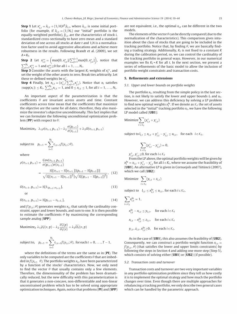
Fig. 1. Surface of objective of (PP) with �1 = 1,�2 = 0 and �3 = 0 with K = 75. The upper surface corresponds to �mkt = 6 and the lower corresponds to �mkt = −6.

Own elaboration.

• maintenance of symbol during the calibration period (i.e., nochange of stock name).

For characteristics, we used market capitalization, alpha andbeta deviation. For market capitalization, for each date t we multi-ply the price of the stock times the number of shares outstanding.For other characteristics, i.e., alpha and beta deviation, we usedt˛w = tˇ

w = 42 trading days to compute the appropriate value of thedefinitions in Section 6. Finally, based on some empirical studies ofDeMiguel, Garlappi, and Uppal (2009), xi,t was considered to be theequally weighted portfolio in Step 1 of Section 4.

7.2. Working with three characteristics: market capitalization,beta deviation and alpha

As noted earlier, we work with three characteristics: marketcapitalization, beta deviation and alpha. Their weights are givenby �mkt,�ˇ and �˛, respectively. Market capitalization was selecteddue to its capacity to explain returns as well as the fact that theS&P500 is a market-capitalization index. Alpha and beta deviationcontain important information about a particular stock relative tothe index. In particular, ˛ is used to assess the ability of a stockto outperform the index and can also be considered as a measureof momentum. Beta is used to assess the risk of the stock comparedto the index. Additionally, both are computed from the same OLSregression, and have been used recently in the enhanced indexationproblem (for example, in Canakgoz and Beasley (2008)). Note thatyˇ in Section 6 was defined as |ˇ−1|. Consequently, low values ofthis characteristic indicate that the particular beta is close to 1, andafter the cross-section normalization it will take negative values.

In this part of the paper, we consider various cases of the objec-tive function in (PP). In the first case, we maximize the correlationcoefficient of the returns of the index and the tracking portfolio, i.e.,�1 = 1, �2 = 0, and �3 = 0. The second case includes in the objectivethe ratio of the standard deviations, i.e., �1 = 1, �2 = 1, and �3 = 0.

While we do not include the enhanced component in these twoinitial cases, we observe different behavior of the objective dueto different effects of the characteristics. These cases are impor-tant since they correspond to versions of a classical index trackingproblem that considers the correlation coefficient and the vari-ance of the tracking portfolio. In particular, we wish to track theS&P500 using 75 stocks (i.e., 15% of its components). To constructthe function f, we follow the steps given in Section 4 using as initialtracking portfolio the equally weighted portfolio. Also, we do notinclude transaction costs, or lower and upper bounds on the portfo-lio weights. The objective is computed using the calibration periodof 124 days corresponding to the trading days between 2011/10/03and 2012/03/30 (as mentioned in the Data section). Since we areusing a calibration period, it is clear that we are using problem(SPP), which is the sample analog of problem (PP).

Figs. 1 and 2 correspond to the case of �1 = 1, �2 = 0, and �3 = 0with K = 75. In Fig. 1, we show two surfaces, the upper one corre-sponds to fixing �mkt = 6 and moving �˛ and �ˇ between −6 and 6in 0.5 steps, and the lower surface corresponds to �mkt = −6 usingthe same range for the other two coefficients. Notice that highervalues of �mkt include stocks with greater presence in the indexin the tracking portfolio. As expected, this fact increases the cor-relation coefficient of the tracking portfolio and the index. With�mkt = 6 we obtain correlation coefficients higher than 0.99; whileusing �mkt = −6, we obtain maximum values that are approximately0.89.

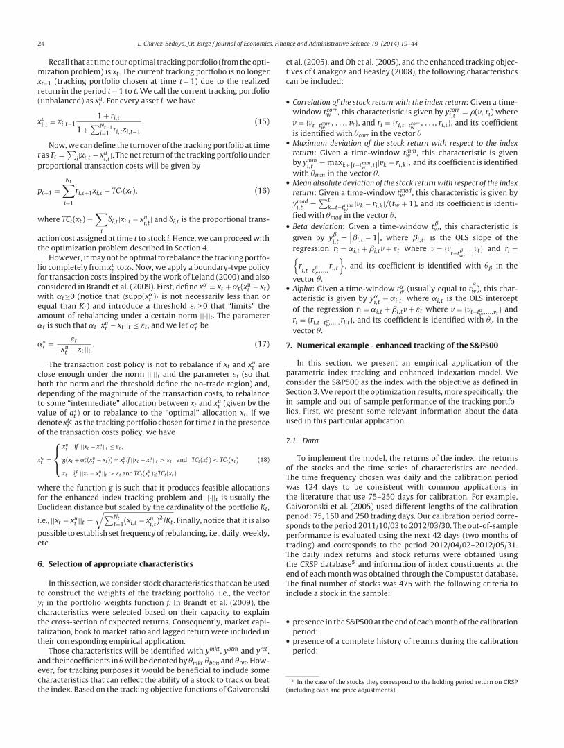
In Fig. 2, we show a color map of the surface correspondingto �mkt = 6. From this figure, we can observe the influence of �ˇ

and �˛ in the maximization of the correlation coefficient. Noticethat the values of �˛ that maximize the objective is centered onzero; therefore, alpha appears to have little relevance for maximiz-ing the correlation coefficient. The case of �ˇ is relatively similar bypresenting values centered at zero for the maximum values of theobjective.

Next, we include in the objective the ratio of the standard devi-ations; recall that by giving weight to this part of the objective

26 L. Chavez-Bedoya, J.R. Birge / Journal of Economics, Finance and Administrative Science 19 (2014) 19–44

0.92

0.93

0.94

0.98

0.99

0.96

0.95

0.97

–6–6

–4

–4

–2

–2

4

2

6

0

42 60

Objective with λ1=1, λ2=0 and λ3=0. Fixing θmkt=6

θβ

θ α

Fig. 2. Color map of the objective of (PP) with �1 = 1, �2 = 0 and �3 = 0 with K = 75 and fixing �mkt = 6.

Own elaboration.

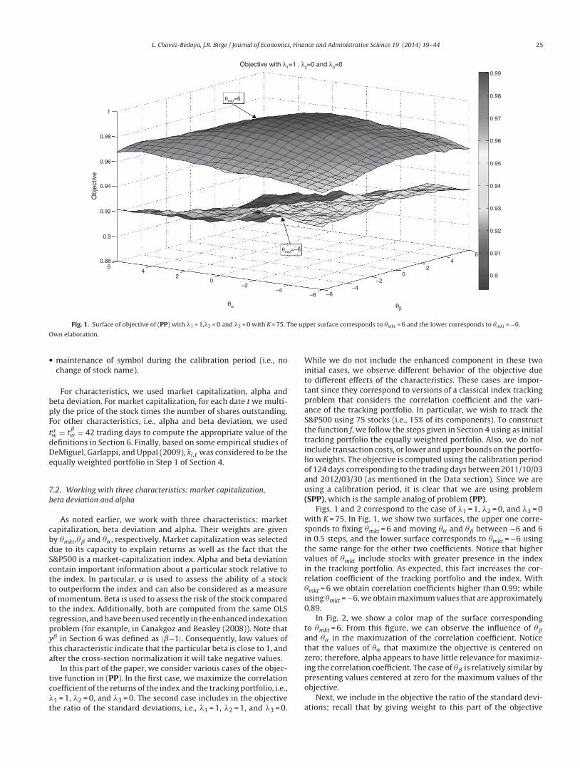
(�2 > 0) we aim to reduce the variance of the tracking portfolio withrespect to the index. For motivational purposes, we now use �1 = 1,�2 = 0, and �3 = 0 and K = 75. The new objective is a more completetracking objective since we both maximize the correlation coeffi-cient and keep the ratio of the variances close to 1. Under the sameconditions as in the previous case, we similarly display Figs. 3 and 4.

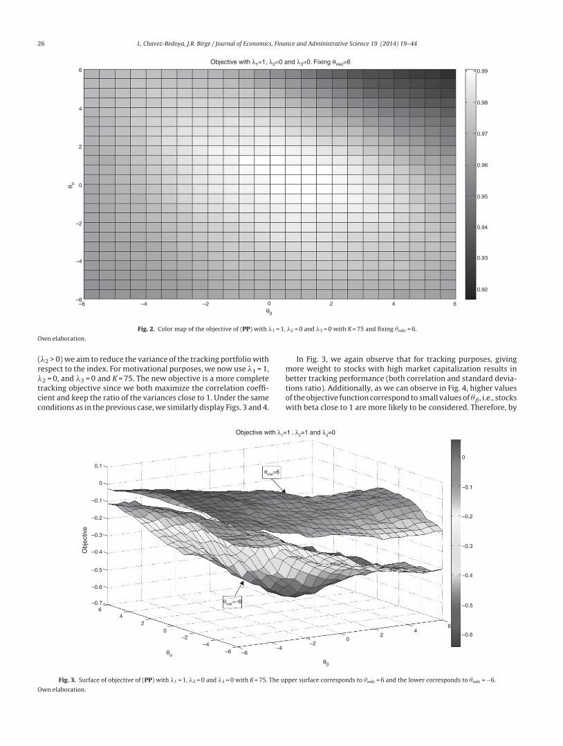
In Fig. 3, we again observe that for tracking purposes, givingmore weight to stocks with high market capitalization results inbetter tracking performance (both correlation and standard devia-tions ratio). Additionally, as we can observe in Fig. 4, higher valuesof the objective function correspond to small values of �ˇ, i.e., stockswith beta close to 1 are more likely to be considered. Therefore, by

–0.6

–0.7

–0.5

–0.4

–0.3

–0.2

–0.1

0.1

0

Obj

ectiv

e

–2–4

–6 –6–4

–20

20

42

6

46

–0.6

–0.5

–0.4

–0.3

–0.2

–0.1

0

θmkt=6

θmkt=–6

θα

θβ

Objective with λ1=1 , λ2=1 and λ3=0

Fig. 3. Surface of objective of (PP) with �1 = 1, �2 = 0 and �3 = 0 with K = 75. The upper surface corresponds to �mkt = 6 and the lower corresponds to �mkt = −6.

Own elaboration.

L. Chavez-Bedoya, J.R. Birge / Journal of Economics, Finance and Administrative Science 19 (2014) 19–44 27

Objective with λ1=1, λ2=1 and λ3=0. Fixing θmkt=6.

–0.2

–0.15

–0.1

–0.05

0

–6–6

–4

–4

–2

–2

4

2

6

0

42 60θβ

θ α

Fig. 4. Color map of the objective of (PP) with �1 = 1, �2 = 1 and �3 = 0 with K = 75 and fixing �mkt = 6.

Own elaboration.

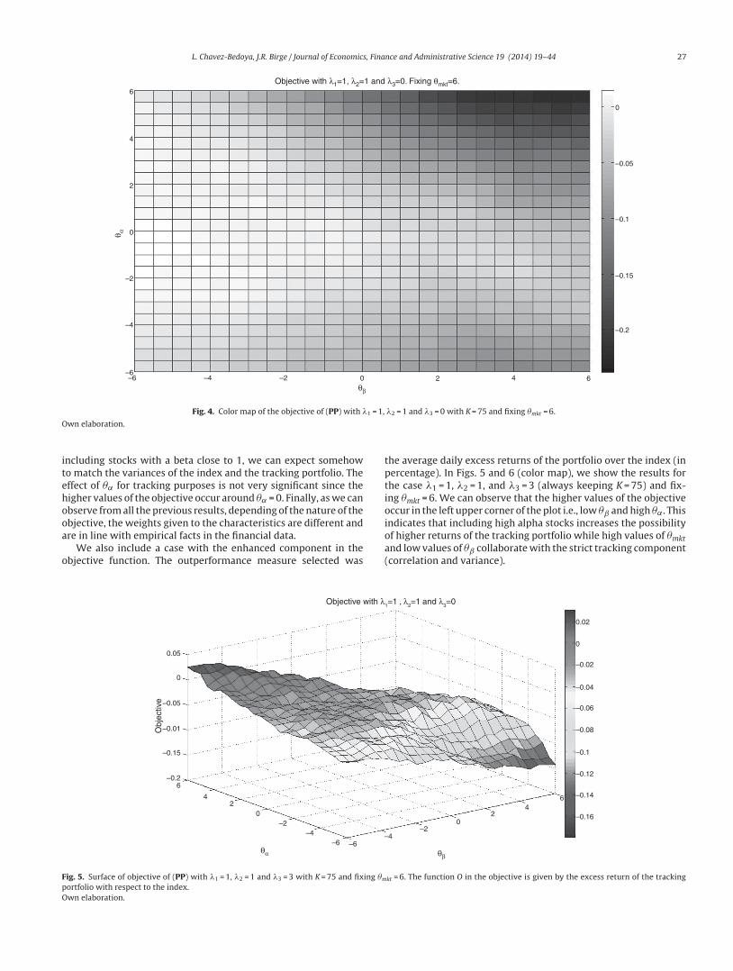
including stocks with a beta close to 1, we can expect somehowto match the variances of the index and the tracking portfolio. Theeffect of �˛ for tracking purposes is not very significant since thehigher values of the objective occur around �˛ = 0. Finally, as we canobserve from all the previous results, depending of the nature of theobjective, the weights given to the characteristics are different andare in line with empirical facts in the financial data.

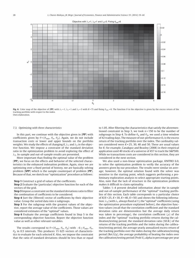
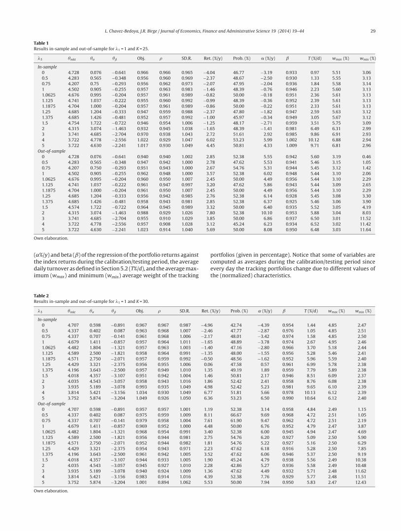
We also include a case with the enhanced component in theobjective function. The outperformance measure selected was

the average daily excess returns of the portfolio over the index (inpercentage). In Figs. 5 and 6 (color map), we show the results forthe case �1 = 1, �2 = 1, and �3 = 3 (always keeping K = 75) and fix-ing �mkt = 6. We can observe that the higher values of the objectiveoccur in the left upper corner of the plot i.e., low �ˇ and high �˛. Thisindicates that including high alpha stocks increases the possibilityof higher returns of the tracking portfolio while high values of �mktand low values of �ˇ collaborate with the strict tracking component(correlation and variance).

–2

–4–6 –6

θα θβ

–4 –20

204

42

6

6–0.2

–0.15

–0.01

–0.05

0.05

0

–0.16

–0.14

–0.12

–0.1

–0.08

–0.06

–0.04

–0.02

0.02

0

Obj

ectiv

e

Objective with λ1=1 , λ2=1 and λ3=0

Fig. 5. Surface of objective of (PP) with �1 = 1, �2 = 1 and �3 = 3 with K = 75 and fixing �mkt = 6. The function O in the objective is given by the excess return of the trackingportfolio with respect to the index.Own elaboration.

28 L. Chavez-Bedoya, J.R. Birge / Journal of Economics, Finance and Administrative Science 19 (2014) 19–44

–0.16

–0.14

–0.12

–0.1

–0.08

–0.06

–0.04

–0.02

0

0.02

–6–6

–4

–4

–2

–2

4

2

6

0

42 60

Objective with λ1=1, λ2=1 and λ3=3. Fixing θmkt=6

θβ

θ α

Fig. 6. Color map of the objective of (PP) with �1 = 1, �2 = 1 and �3 = 3 with K = 75 and fixing �mkt = 6. The function O in the objective is given by the excess return of thetracking portfolio with respect to the index.Own elaboration.

7.3. Optimizing with three characteristics

In this part, we continue with the objective given in (PP) withcoefficients given by � = (�mkt, �˛, �ˇ). Again, we do not includetransaction costs or lower and upper bounds on the portfolioweights. We study the effects of changing K, �1 and �3 in the objec-tive function. We impose a constraint of the standard deviationratio in the optimization problem to avoid exploring the effect of�2. In-sample and out-of-sample results are presented.

More important than finding the optimal value of the problem(PP), we focus on the effects and behavior of the selected charac-teristics in the enhanced indexation problem. Again, since we areoptimizing over a fixed period of history, we are basically solvingproblem (SPP) which is the sample counterpart of problem (PP).Because of that, we sketch our “optimization” procedure as follows:

Step 1 Construct a grid of values of the coefficients.Step 2 Evaluate the (particular) objective function for each of thevectors of the grid.Step 3 Impose a constraint on the standard deviations ratio to filterthe combination of coefficients to be considered.Step 4 Sort the (filtered) vector of coefficients by their objectivevalue. Group the sorted data into n subgroups.Step 5 For the subgroup with the greatest values of the objec-tive, report the average value of the coefficients. Those values areconsidered estimates of the “optimal” values.Step 6 Evaluate the average coefficients found in Step 5 in thecorresponding objective function. Report the objective functionvalue as well as other relevant variables.

The results correspond to � = (�mkt, �˛, �ˇ) with −6 ≤ �mkt, �˛,�ˇ in 0.5 intervals. This produces 15 625 vectors of characteris-tics to evaluate for each selected K. Also, we impose the constraintthat the ratio of standard deviations should be less than or equal

to 1.05. After filtering the characteristics that satisfy the aforemen-tioned constraint in Step 3, we took n = 150 to be the number ofsubgroups in Step 4. To define �˛ and �ˇ, we used a time windowof 42 trading days. The measure of out-performance Ot is the excessreturn of the tracking portfolio over the index. The cardinality val-ues considered were K = 25, 30, 40 and 50. These are usual valuesfor K; for example, Canakgoz and Beasley (2008) in their empiricalapplication used 40 stocks of a universe of 457 to track the S&P500.While no transactions costs are considered in this section, they areconsidered in the next section.

We also used a non-linear optimization package, KNITRO 6.0,to solve the optimization problem to verify the accuracy of theanswers given by our procedure. The results were similar on aver-age; however, the optimal solution found with the solver wassensitive to the starting point, which suggests performing a pre-liminary exploration analysis to select appropriate starting points.Also, note that the lack of structure in the optimization problemmakes it difficult to claim optimality.

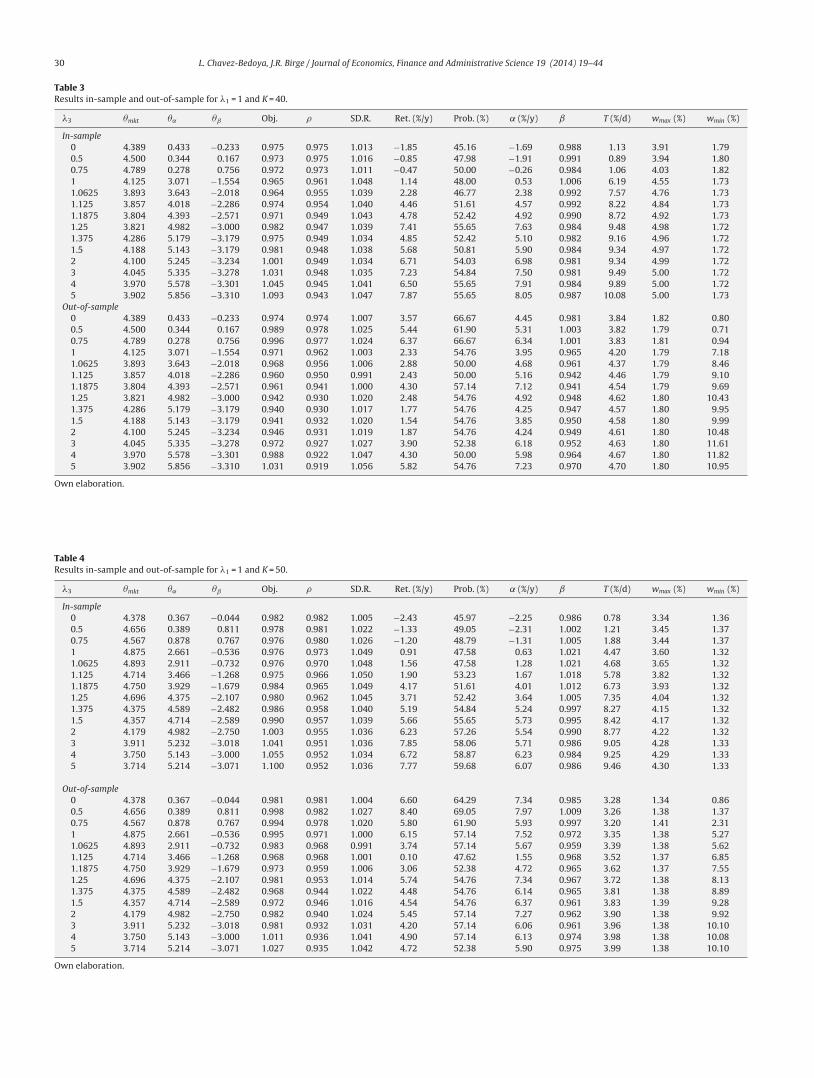
Tables 1–4 present detailed information about the in-sampleand out-of-sample performance of the “optimal” tracking portfo-lios of this section. Each table corresponds to a particular choiceof K(K = 25, K = 30, K = 40, K = 50) and shows the following informa-tion: �3 (with �1 always fixed at 1), the “optimal” coefficients (usingthe optimization procedure explained before), the objective func-tion values (recall that the correlation coefficient and the standarddeviation ratio are dimensionless but the average daily returnwas taken in percentage), the correlation coefficient (�) of theindex and the “optimal” tracking portfolio returns during the cal-ibration/testing period, the standard deviation ratio (SD.R.) of thereturns of the tracking portfolio and the index during the calibra-tion/testing period, the average yearly annualized excess return ofthe tracking portfolio over the index during the calibration/testingperiod (Ret.%/y), the average probability of beating the index overthe calibration/testing period (Prob %), alpha in percentage per year

L. Chavez-Bedoya, J.R. Birge / Journal of Economics, Finance and Administrative Science 19 (2014) 19–44 29

Table 1Results in-sample and out-of-sample for �1 = 1 and K = 25.

�3 �mkt �˛ �ˇ Obj. � SD.R. Ret. (%/y) Prob. (%) � (%/y) ˇ T (%/d) wman (%) wmin (%)

In-sample0 4.728 0.076 −0.641 0.966 0.966 0.965 −4.04 46.77 −3.19 0.933 0.97 5.51 3.060.5 4.283 0.565 −0.348 0.956 0.960 0.969 −2.37 48.67 −2.50 0.930 1.33 5.55 3.130.75 4.207 0.75 −0.293 0.956 0.962 0.973 −2.07 47.95 −2.04 0.936 1.84 5.58 3.141 4.502 0.905 −0.255 0.957 0.963 0.983 −1.46 48.39 −0.76 0.946 2.23 5.60 3.131.0625 4.676 0.995 −0.204 0.957 0.961 0.989 −0.82 50.00 −0.18 0.951 2.36 5.61 3.131.125 4.741 1.037 −0.222 0.955 0.960 0.992 −0.99 48.39 −0.36 0.952 2.39 5.61 3.131.1875 4.704 1.000 −0.204 0.957 0.961 0.989 −0.86 50.00 −0.22 0.951 2.33 5.61 3.131.25 4.685 1.204 −0.333 0.947 0.959 0.988 −2.37 47.80 −1.82 0.947 2.59 5.63 3.121.375 4.685 1.426 −0.481 0.952 0.957 0.992 −1.00 45.97 −0.34 0.949 3.05 5.67 3.121.5 4.754 1.722 −0.722 0.946 0.954 1.006 −1.25 48.17 −2.71 0.959 3.51 5.75 3.092 4.315 3.074 −1.463 0.932 0.945 1.038 −1.65 48.39 −1.41 0.981 6.49 6.31 2.993 3.741 4.685 −2.704 0.970 0.938 1.043 2.72 51.61 2.92 0.985 9.86 6.91 2.934 3.722 4.778 −2.556 1.022 0.929 1.047 6.02 53.23 5.99 1.002 10.12 6.88 2.945 3.722 4.630 −2.241 1.017 0.930 1.049 4.45 50.81 4.33 1.009 9.71 6.81 2.96

Out-of-sample0 4.728 0.076 −0.641 0.940 0.940 1.002 2.85 52.38 5.55 0.942 5.60 3.19 0.460.5 4.283 0.565 −0.348 0.947 0.942 1.000 2.78 47.62 5.53 0.941 5.46 3.15 1.050.75 4.207 0.750 −0.293 0.951 0.943 1.000 2.67 54.76 5.31 0.944 5.45 3.12 1.421 4.502 0.905 −0.255 0.962 0.948 1.000 3.57 52.38 6.02 0.948 5.44 3.10 2.061.0625 4.676 0.995 −0.204 0.960 0.950 1.007 2.45 50.00 4.49 0.956 5.44 3.10 2.291.125 4.741 1.037 −0.222 0.961 0.947 0.997 3.20 47.62 5.86 0.943 5.44 3.09 2.651.1875 4.704 1.000 −0.204 0.961 0.950 1.007 2.45 50.00 4.49 0.956 5.44 3.10 2.291.25 4.685 1.204 −0.333 0.956 0.942 0.985 2.76 52.38 6.14 0.928 5.45 3.08 3.301.375 4.685 1.426 −0.481 0.958 0.943 0.981 2.85 52.38 6.37 0.925 5.46 3.06 3.901.5 4.574 1.722 −0.722 0.964 0.945 0.989 3.32 50.00 6.40 0.935 5.52 3.05 4.192 4.315 3.074 −1.463 0.988 0.929 1.026 7.80 52.38 10.10 0.953 5.88 3.04 8.033 3.741 4.685 −2.704 0.955 0.910 1.029 3.85 50.00 6.86 0.937 6.50 3.01 11.524 3.722 4.778 −2.556 0.957 0.908 1.028 3.12 45.24 6.23 0.934 6.52 3.02 11.425 3.722 4.630 −2.241 1.023 0.914 1.040 5.69 50.00 8.08 0.950 6.48 3.03 11.64

Own elaboration.

(˛%/y) and beta (ˇ) of the regression of the portfolio returns againstthe index returns during the calibration/testing period, the averagedaily turnover as defined in Section 5.2 (T%/d), and the average max-imum (wmax) and minimum (wmin) average weight of the tracking

portfolios (given in percentage). Notice that some of variables arecomputed as averages during the calibration/testing period sinceevery day the tracking portfolios change due to different values ofthe (normalized) characteristics.

Table 2Results in-sample and out-of-sample for �1 = 1 and K = 30.

�3 �mkt �˛ �ˇ Obj. � SD.R. Ret. (%/y) Prob. (%) ˛ (%/y) ˇ T (%/d) wmax (%) wmin (%)

In-sample0 4.707 0.598 −0.891 0.967 0.967 0.987 −4.96 42.74 −4.39 0.954 1.44 4.85 2.470.5 4.337 0.402 0.087 0.963 0.968 1.007 −2.46 47.77 −2.87 0.976 1.05 4.85 2.510.75 4.337 0.707 −0.141 0.961 0.968 1.006 −2.17 48.01 −3.42 0.974 1.58 4.85 2.501 4.679 1.411 −0.857 0.957 0.964 1.011 −1.65 48.89 −3.78 0.974 2.67 4.95 2.461.0625 4.482 1.804 −1.321 0.957 0.963 1.003 −1.40 47.16 −2.80 0.966 3.70 5.18 2.441.125 4.589 2.500 −1.821 0.958 0.964 0.991 −1.35 48.00 −1.55 0.956 5.28 5.46 2.411.1875 4.571 2.750 −2.071 0.957 0.959 0.992 −0.50 48.56 −1.62 0.952 5.96 5.59 2.401.25 4.429 3.321 −2.375 0.956 0.955 1.006 0.06 47.58 0.57 0.961 6.99 5.78 2.381.375 4.196 3.643 −2.500 0.957 0.949 1.010 1.35 49.19 1.89 0.959 7.79 5.89 2.381.5 4.018 4.357 −3.107 0.951 0.942 1.004 1.46 50.81 2.17 0.946 8.51 6.09 2.372 4.035 4.543 −3.057 0.958 0.943 1.016 1.86 52.42 2.41 0.958 8.76 6.08 2.383 3.935 5.189 −3.078 0.993 0.935 1.049 4.98 52.42 5.23 0.981 9.65 6.10 2.394 3.814 5.421 −3.156 1.034 0.930 1.049 6.77 51.81 5.66 0.978 10.13 6.12 2.395 3.752 5.874 −3.204 1.049 0.926 1.050 6.36 53.23 6.50 0.990 10.64 6.12 2.40

Out-of-sample0 4.707 0.598 −0.891 0.957 0.957 1.001 1.19 52.38 3.14 0.958 4.84 2.49 1.150.5 4.337 0.402 0.087 0.975 0.959 1.009 8.11 66.67 9.69 0.968 4.72 2.51 1.050.75 4.337 0.707 −0.141 0.979 0.958 1.004 7.61 61.90 9.47 0.962 4.72 2.51 2.191 4.679 1.411 −0.857 0.969 0.952 1.000 4.48 50.00 6.76 0.952 4.79 2.47 3.871.0625 4.482 1.804 −1.321 0.968 0.954 0.991 3.40 52.38 6.00 0.945 4.94 2.47 4.691.125 4.589 2.500 −1.821 0.956 0.944 0.981 2.75 54.76 6.20 0.927 5.09 2.50 5.901.1875 4.571 2.750 −2.071 0.952 0.944 0.982 1.81 54.76 5.22 0.927 5.16 2.50 6.291.25 4.429 3.321 −2.375 0.954 0.943 0.971 2.23 47.62 6.18 0.916 5.28 2.50 7.851.375 4.196 3.643 −2.500 0.961 0.942 1.005 3.52 47.62 6.06 0.946 5.37 2.50 9.191.5 4.018 4.357 −3.107 0.944 0.933 1.005 1.90 45.24 4.79 0.938 5.56 2.49 10.382 4.035 4.543 −3.057 0.945 0.927 1.010 2.28 42.86 5.27 0.936 5.58 2.49 10.483 3.935 5.189 −3.078 0.940 0.924 1.009 1.36 47.62 4.49 0.932 5.71 2.48 11.624 3.814 5.421 −3.156 0.983 0.914 1.016 4.39 52.38 7.76 0.929 5.77 2.48 11.515 3.752 5.874 −3.204 1.001 0.894 1.062 5.53 50.00 7.94 0.950 5.83 2.47 12.43

Own elaboration.

30 L. Chavez-Bedoya, J.R. Birge / Journal of Economics, Finance and Administrative Science 19 (2014) 19–44

Table 3Results in-sample and out-of-sample for �1 = 1 and K = 40.

�3 �mkt �˛ �ˇ Obj. � SD.R. Ret. (%/y) Prob. (%) ˛ (%/y) ˇ T (%/d) wmax (%) wmin (%)

In-sample0 4.389 0.433 −0.233 0.975 0.975 1.013 −1.85 45.16 −1.69 0.988 1.13 3.91 1.790.5 4.500 0.344 0.167 0.973 0.975 1.016 −0.85 47.98 −1.91 0.991 0.89 3.94 1.800.75 4.789 0.278 0.756 0.972 0.973 1.011 −0.47 50.00 −0.26 0.984 1.06 4.03 1.821 4.125 3.071 −1.554 0.965 0.961 1.048 1.14 48.00 0.53 1.006 6.19 4.55 1.731.0625 3.893 3.643 −2.018 0.964 0.955 1.039 2.28 46.77 2.38 0.992 7.57 4.76 1.731.125 3.857 4.018 −2.286 0.974 0.954 1.040 4.46 51.61 4.57 0.992 8.22 4.84 1.731.1875 3.804 4.393 −2.571 0.971 0.949 1.043 4.78 52.42 4.92 0.990 8.72 4.92 1.731.25 3.821 4.982 −3.000 0.982 0.947 1.039 7.41 55.65 7.63 0.984 9.48 4.98 1.721.375 4.286 5.179 −3.179 0.975 0.949 1.034 4.85 52.42 5.10 0.982 9.16 4.96 1.721.5 4.188 5.143 −3.179 0.981 0.948 1.038 5.68 50.81 5.90 0.984 9.34 4.97 1.722 4.100 5.245 −3.234 1.001 0.949 1.034 6.71 54.03 6.98 0.981 9.34 4.99 1.723 4.045 5.335 −3.278 1.031 0.948 1.035 7.23 54.84 7.50 0.981 9.49 5.00 1.724 3.970 5.578 −3.301 1.045 0.945 1.041 6.50 55.65 7.91 0.984 9.89 5.00 1.725 3.902 5.856 −3.310 1.093 0.943 1.047 7.87 55.65 8.05 0.987 10.08 5.00 1.73

Out-of-sample0 4.389 0.433 −0.233 0.974 0.974 1.007 3.57 66.67 4.45 0.981 3.84 1.82 0.800.5 4.500 0.344 0.167 0.989 0.978 1.025 5.44 61.90 5.31 1.003 3.82 1.79 0.710.75 4.789 0.278 0.756 0.996 0.977 1.024 6.37 66.67 6.34 1.001 3.83 1.81 0.941 4.125 3.071 −1.554 0.971 0.962 1.003 2.33 54.76 3.95 0.965 4.20 1.79 7.181.0625 3.893 3.643 −2.018 0.968 0.956 1.006 2.88 50.00 4.68 0.961 4.37 1.79 8.461.125 3.857 4.018 −2.286 0.960 0.950 0.991 2.43 50.00 5.16 0.942 4.46 1.79 9.101.1875 3.804 4.393 −2.571 0.961 0.941 1.000 4.30 57.14 7.12 0.941 4.54 1.79 9.691.25 3.821 4.982 −3.000 0.942 0.930 1.020 2.48 54.76 4.92 0.948 4.62 1.80 10.431.375 4.286 5.179 −3.179 0.940 0.930 1.017 1.77 54.76 4.25 0.947 4.57 1.80 9.951.5 4.188 5.143 −3.179 0.941 0.932 1.020 1.54 54.76 3.85 0.950 4.58 1.80 9.992 4.100 5.245 −3.234 0.946 0.931 1.019 1.87 54.76 4.24 0.949 4.61 1.80 10.483 4.045 5.335 −3.278 0.972 0.927 1.027 3.90 52.38 6.18 0.952 4.63 1.80 11.614 3.970 5.578 −3.301 0.988 0.922 1.047 4.30 50.00 5.98 0.964 4.67 1.80 11.825 3.902 5.856 −3.310 1.031 0.919 1.056 5.82 54.76 7.23 0.970 4.70 1.80 10.95

Own elaboration.

Table 4Results in-sample and out-of-sample for �1 = 1 and K = 50.

�3 �mkt �˛ �ˇ Obj. � SD.R. Ret. (%/y) Prob. (%) ˛ (%/y) ˇ T (%/d) wmax (%) wmin (%)

In-sample0 4.378 0.367 −0.044 0.982 0.982 1.005 −2.43 45.97 −2.25 0.986 0.78 3.34 1.360.5 4.656 0.389 0.811 0.978 0.981 1.022 −1.33 49.05 −2.31 1.002 1.21 3.45 1.370.75 4.567 0.878 0.767 0.976 0.980 1.026 −1.20 48.79 −1.31 1.005 1.88 3.44 1.371 4.875 2.661 −0.536 0.976 0.973 1.049 0.91 47.58 0.63 1.021 4.47 3.60 1.321.0625 4.893 2.911 −0.732 0.976 0.970 1.048 1.56 47.58 1.28 1.021 4.68 3.65 1.321.125 4.714 3.466 −1.268 0.975 0.966 1.050 1.90 53.23 1.67 1.018 5.78 3.82 1.321.1875 4.750 3.929 −1.679 0.984 0.965 1.049 4.17 51.61 4.01 1.012 6.73 3.93 1.321.25 4.696 4.375 −2.107 0.980 0.962 1.045 3.71 52.42 3.64 1.005 7.35 4.04 1.321.375 4.375 4.589 −2.482 0.986 0.958 1.040 5.19 54.84 5.24 0.997 8.27 4.15 1.321.5 4.357 4.714 −2.589 0.990 0.957 1.039 5.66 55.65 5.73 0.995 8.42 4.17 1.322 4.179 4.982 −2.750 1.003 0.955 1.036 6.23 57.26 5.54 0.990 8.77 4.22 1.323 3.911 5.232 −3.018 1.041 0.951 1.036 7.85 58.06 5.71 0.986 9.05 4.28 1.334 3.750 5.143 −3.000 1.055 0.952 1.034 6.72 58.87 6.23 0.984 9.25 4.29 1.335 3.714 5.214 −3.071 1.100 0.952 1.036 7.77 59.68 6.07 0.986 9.46 4.30 1.33

Out-of-sample0 4.378 0.367 −0.044 0.981 0.981 1.004 6.60 64.29 7.34 0.985 3.28 1.34 0.860.5 4.656 0.389 0.811 0.998 0.982 1.027 8.40 69.05 7.97 1.009 3.26 1.38 1.370.75 4.567 0.878 0.767 0.994 0.978 1.020 5.80 61.90 5.93 0.997 3.20 1.41 2.311 4.875 2.661 −0.536 0.995 0.971 1.000 6.15 57.14 7.52 0.972 3.35 1.38 5.271.0625 4.893 2.911 −0.732 0.983 0.968 0.991 3.74 57.14 5.67 0.959 3.39 1.38 5.621.125 4.714 3.466 −1.268 0.968 0.968 1.001 0.10 47.62 1.55 0.968 3.52 1.37 6.851.1875 4.750 3.929 −1.679 0.973 0.959 1.006 3.06 52.38 4.72 0.965 3.62 1.37 7.551.25 4.696 4.375 −2.107 0.981 0.953 1.014 5.74 54.76 7.34 0.967 3.72 1.38 8.131.375 4.375 4.589 −2.482 0.968 0.944 1.022 4.48 54.76 6.14 0.965 3.81 1.38 8.891.5 4.357 4.714 −2.589 0.972 0.946 1.016 4.54 54.76 6.37 0.961 3.83 1.39 9.282 4.179 4.982 −2.750 0.982 0.940 1.024 5.45 57.14 7.27 0.962 3.90 1.38 9.923 3.911 5.232 −3.018 0.981 0.932 1.031 4.20 57.14 6.06 0.961 3.96 1.38 10.104 3.750 5.143 −3.000 1.011 0.936 1.041 4.90 57.14 6.13 0.974 3.98 1.38 10.085 3.714 5.214 −3.071 1.027 0.935 1.042 4.72 52.38 5.90 0.975 3.99 1.38 10.10

Own elaboration.

L. Chavez-Bedoya, J.R. Birge / Journal of Economics, Finance and Administrative Science 19 (2014) 19–44 31

0

–4

–2

0

2

4

6

K=25 K=30

K=50K=40

0.5 1 1.5 2 3 4 53.5 4.52.5

θmkt

θα

θβ

λ3

0

–4

–2

0

2

4

6

0.5 1 1.5 2 3 4 53.5 4.52.5

θmkt

θα

θβ

λ3

0

–4

–2

0

2

4

6

0.5 1 1.5 2 3 4 53.5 4.52.5

θmkt

θα

θβ

λ3

0

–4

–2

0

2

4

6

0.5 1 1.5 2 3 4 53.5 4.52.5

θmkt

θα

θβ

λ3

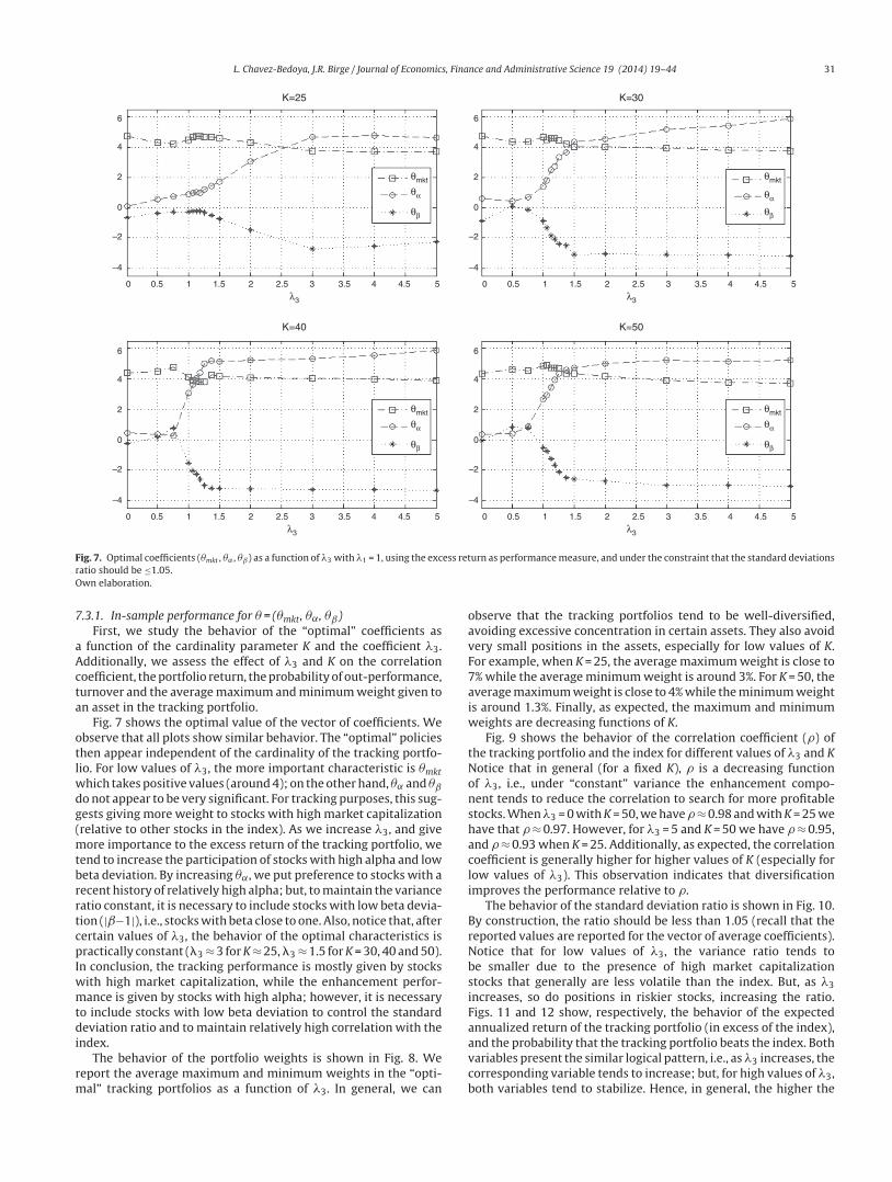
Fig. 7. Optimal coefficients (�mkt , �˛ , �ˇ) as a function of �3 with �1 = 1, using the excess return as performance measure, and under the constraint that the standard deviationsratio should be ≤1.05.Own elaboration.

7.3.1. In-sample performance for � = (�mkt, �˛, �ˇ)First, we study the behavior of the “optimal” coefficients as

a function of the cardinality parameter K and the coefficient �3.Additionally, we assess the effect of �3 and K on the correlationcoefficient, the portfolio return, the probability of out-performance,turnover and the average maximum and minimum weight given toan asset in the tracking portfolio.

Fig. 7 shows the optimal value of the vector of coefficients. Weobserve that all plots show similar behavior. The “optimal” policiesthen appear independent of the cardinality of the tracking portfo-lio. For low values of �3, the more important characteristic is �mktwhich takes positive values (around 4); on the other hand, �˛ and �ˇ

do not appear to be very significant. For tracking purposes, this sug-gests giving more weight to stocks with high market capitalization(relative to other stocks in the index). As we increase �3, and givemore importance to the excess return of the tracking portfolio, wetend to increase the participation of stocks with high alpha and lowbeta deviation. By increasing �˛, we put preference to stocks with arecent history of relatively high alpha; but, to maintain the varianceratio constant, it is necessary to include stocks with low beta devia-tion (|ˇ−1|), i.e., stocks with beta close to one. Also, notice that, aftercertain values of �3, the behavior of the optimal characteristics ispractically constant (�3 ≈ 3 for K ≈ 25, �3 ≈ 1.5 for K = 30, 40 and 50).In conclusion, the tracking performance is mostly given by stockswith high market capitalization, while the enhancement perfor-mance is given by stocks with high alpha; however, it is necessaryto include stocks with low beta deviation to control the standarddeviation ratio and to maintain relatively high correlation with theindex.

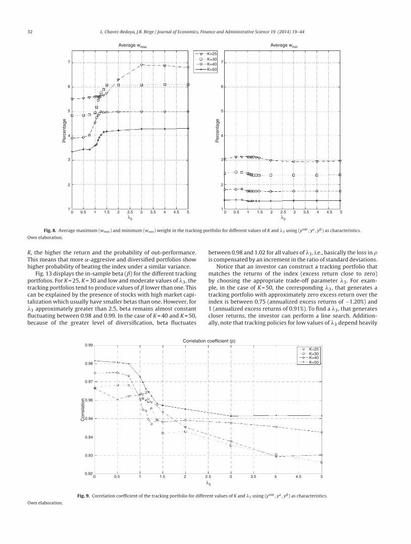
The behavior of the portfolio weights is shown in Fig. 8. Wereport the average maximum and minimum weights in the “opti-mal” tracking portfolios as a function of �3. In general, we can

observe that the tracking portfolios tend to be well-diversified,avoiding excessive concentration in certain assets. They also avoidvery small positions in the assets, especially for low values of K.For example, when K = 25, the average maximum weight is close to7% while the average minimum weight is around 3%. For K = 50, theaverage maximum weight is close to 4% while the minimum weightis around 1.3%. Finally, as expected, the maximum and minimumweights are decreasing functions of K.

Fig. 9 shows the behavior of the correlation coefficient (�) ofthe tracking portfolio and the index for different values of �3 and KNotice that in general (for a fixed K), � is a decreasing functionof �3, i.e., under “constant” variance the enhancement compo-nent tends to reduce the correlation to search for more profitablestocks. When �3 = 0 with K = 50, we have � ≈ 0.98 and with K = 25 wehave that � ≈ 0.97. However, for �3 = 5 and K = 50 we have � ≈ 0.95,and � ≈ 0.93 when K = 25. Additionally, as expected, the correlationcoefficient is generally higher for higher values of K (especially forlow values of �3). This observation indicates that diversificationimproves the performance relative to �.

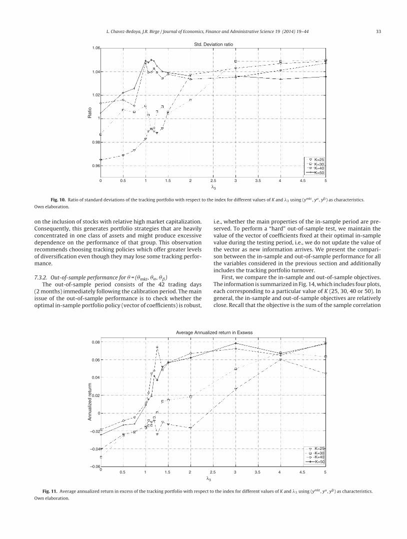
The behavior of the standard deviation ratio is shown in Fig. 10.By construction, the ratio should be less than 1.05 (recall that thereported values are reported for the vector of average coefficients).Notice that for low values of �3, the variance ratio tends tobe smaller due to the presence of high market capitalizationstocks that generally are less volatile than the index. But, as �3increases, so do positions in riskier stocks, increasing the ratio.Figs. 11 and 12 show, respectively, the behavior of the expectedannualized return of the tracking portfolio (in excess of the index),and the probability that the tracking portfolio beats the index. Bothvariables present the similar logical pattern, i.e., as �3 increases, thecorresponding variable tends to increase; but, for high values of �3,both variables tend to stabilize. Hence, in general, the higher the

32 L. Chavez-Bedoya, J.R. Birge / Journal of Economics, Finance and Administrative Science 19 (2014) 19–44

01

2

3

4

5

6

7

K=25K=30K=40K=50

Average wmax Average wmin

Per

cent

age

0.5 1 1.5 2 3 43.5 4.5 52.5λ3

01

2

3

4

5

6

7

Per

cent

age

0.5 1 1.5 2 3 43.5 4.5 52.5λ3

Fig. 8. Average maximum (wmax) and minimum (wmin) weight in the tracking portfolio for different values of K and �3 using (ymkt , y˛ , y�) as characteristics.

Own elaboration.

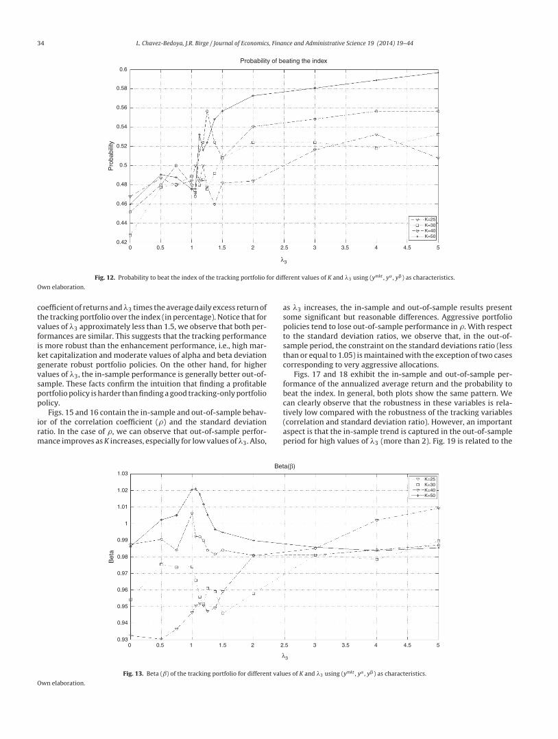
K, the higher the return and the probability of out-performance.This means that more ˛-aggresive and diversified portfolios showhigher probability of beating the index under a similar variance.

Fig. 13 displays the in-sample beta (ˇ) for the different trackingportfolios. For K = 25, K = 30 and low and moderate values of �3, thetracking portfolios tend to produce values of ˇ lower than one. Thiscan be explained by the presence of stocks with high market capi-talization which usually have smaller betas than one. However, for�3 approximately greater than 2.5, beta remains almost constantfluctuating between 0.98 and 0.99. In the case of K = 40 and K = 50,because of the greater level of diversification, beta fluctuates

between 0.98 and 1.02 for all values of �3, i.e., basically the loss in �is compensated by an increment in the ratio of standard deviations.

Notice that an investor can construct a tracking portfolio thatmatches the returns of the index (excess return close to zero)by choosing the appropriate trade-off parameter �3. For exam-ple, in the case of K = 50, the corresponding �3, that generates atracking portfolio with approximately zero excess return over theindex is between 0.75 (annualized excess returns of −1.20%) and1 (annualized excess returns of 0.91%). To find a �3, that generatescloser returns, the investor can perform a line search. Addition-ally, note that tracking policies for low values of �3 depend heavily

00.92

0.93

0.94

0.94

0.96

0.97

0.98

0.99K=25K=30K=40K=50

Correlation coefficient (p)

Cor

rela

tion

0.5 1 1.5 2 3 43.5 4.5 52.5

λ3

Fig. 9. Correlation coefficient of the tracking portfolio for different values of K and �3 using (ymkt , y˛ , y�) as characteristics.

Own elaboration.

L. Chavez-Bedoya, J.R. Birge / Journal of Economics, Finance and Administrative Science 19 (2014) 19–44 33

0

0.96

0.98

1

1.02

1.04

1.06

K=25K=30K=40K=50

Std. Deviation ratio

Rat

io

0.5 1 1.5 2 3 43.5 4.5 52.5

λ3

Fig. 10. Ratio of standard deviations of the tracking portfolio with respect to the index for different values of K and �3 using (ymkt , y˛ , y�) as characteristics.

Own elaboration.

on the inclusion of stocks with relative high market capitalization.Consequently, this generates portfolio strategies that are heavilyconcentrated in one class of assets and might produce excessivedependence on the performance of that group. This observationrecommends choosing tracking policies which offer greater levelsof diversification even though they may lose some tracking perfor-mance.

7.3.2. Out-of-sample performance for � = (�mkt, �˛, �ˇ)The out-of-sample period consists of the 42 trading days

(2 months) immediately following the calibration period. The mainissue of the out-of-sample performance is to check whether theoptimal in-sample portfolio policy (vector of coefficients) is robust,

i.e., whether the main properties of the in-sample period are pre-served. To perform a “hard” out-of-sample test, we maintain thevalue of the vector of coefficients fixed at their optimal in-samplevalue during the testing period, i.e., we do not update the value ofthe vector as new information arrives. We present the compari-son between the in-sample and out-of-sample performance for allthe variables considered in the previous section and additionallyincludes the tracking portfolio turnover.

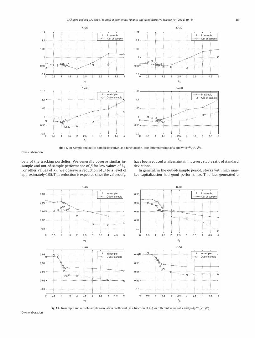
First, we compare the in-sample and out-of-sample objectives.The information is summarized in Fig. 14, which includes four plots,each corresponding to a particular value of K (25, 30, 40 or 50). Ingeneral, the in-sample and out-of-sample objectives are relativelyclose. Recall that the objective is the sum of the sample correlation

0–0.06

–0.04

–0.02

0

0.02

0.04

0.06

0.08

K=25K=30K=40K=50

Average Annualized return in Exswss

Ann

ualiz

ed r

etur

m

0.5 1 1.5 2 3 43.5 4.5 52.5

λ3

Fig. 11. Average annualized return in excess of the tracking portfolio with respect to the index for different values of K and �3 using (ymkt , y˛ , y�) as characteristics.

Own elaboration.

34 L. Chavez-Bedoya, J.R. Birge / Journal of Economics, Finance and Administrative Science 19 (2014) 19–44

0.6

0.58

0.56

0.54

0.52

Pro

babi

lity

0.5

0.48

0.46

0.44

0.420 0.5 1 1.5 2 2.5 3 3.5 4 4.5 5

λ3

K=25

Probability of beating the index

K=30K=40K=50

Fig. 12. Probability to beat the index of the tracking portfolio for different values of K and �3 using (ymkt , y˛ , y�) as characteristics.

Own elaboration.

coefficient of returns and �3 times the average daily excess return ofthe tracking portfolio over the index (in percentage). Notice that forvalues of �3 approximately less than 1.5, we observe that both per-formances are similar. This suggests that the tracking performanceis more robust than the enhancement performance, i.e., high mar-ket capitalization and moderate values of alpha and beta deviationgenerate robust portfolio policies. On the other hand, for highervalues of �3, the in-sample performance is generally better out-of-sample. These facts confirm the intuition that finding a profitableportfolio policy is harder than finding a good tracking-only portfoliopolicy.

Figs. 15 and 16 contain the in-sample and out-of-sample behav-ior of the correlation coefficient (�) and the standard deviationratio. In the case of �, we can observe that out-of-sample perfor-mance improves as K increases, especially for low values of �3. Also,

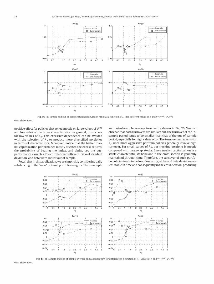
as �3 increases, the in-sample and out-of-sample results presentsome significant but reasonable differences. Aggressive portfoliopolicies tend to lose out-of-sample performance in �. With respectto the standard deviation ratios, we observe that, in the out-of-sample period, the constraint on the standard deviations ratio (lessthan or equal to 1.05) is maintained with the exception of two casescorresponding to very aggressive allocations.

Figs. 17 and 18 exhibit the in-sample and out-of-sample per-formance of the annualized average return and the probability tobeat the index. In general, both plots show the same pattern. Wecan clearly observe that the robustness in these variables is rela-tively low compared with the robustness of the tracking variables(correlation and standard deviation ratio). However, an importantaspect is that the in-sample trend is captured in the out-of-sampleperiod for high values of �3 (more than 2). Fig. 19 is related to the

1.03

1.02

1.01

1

0.99

0.98

Bet

a

0.97

0.96

0.95

0.94

0.930 0.5 1 1.5 2 2.5 3 3.5 4 4.5 5

Beta(β)

K=25K=30K=40K=50

λ3

Fig. 13. Beta (ˇ) of the tracking portfolio for different values of K and �3 using (ymkt , y˛ , y�) as characteristics.

Own elaboration.

L. Chavez-Bedoya, J.R. Birge / Journal of Economics, Finance and Administrative Science 19 (2014) 19–44 35

1.15

1.1

1.05

1

0.95

0.9

1.15

1.1

1.05

1

0.95

0.9

1.15

1.1

1

1.05

0.95

0.9

1.15

1.1

1

1.05

0.95

0.9

0 0.5 1 1.5 2 2.5

λ3 λ3

λ3 λ3

3 3.5 4 4.5 5 0 0.5 1 1.5 2 2.5 3 3.5 4 4.5 5

0 0.5 1 1.5 2 2.5 3 3.5 4 4.5 50 0.5 1 1.5 2 2.5 3 3.5 4 4.5 5

K=25 K=30

In sampleOut of sample

In sampleOut of sample

In sampleOut of sample

In sample

K=40 K=50

Out of sample

Fig. 14. In-sample and out-of-sample objective (as a function of �3) for different values of K and y = (ymkt , y˛ , y�).

Own elaboration.

beta of the tracking portfolios. We generally observe similar in-sample and out-of-sample performance of ˇ for low values of �3.For other values of �3, we observe a reduction of ˇ to a level ofapproximately 0.95. This reduction is expected since the values of �

have been reduced while maintaining a very stable ratio of standarddeviations.

In general, in the out-of-sample period, stocks with high mar-ket capitalization had good performance. This fact generated a

0.98

0.96

0.94

0.92

0.9

0.98

0.96

0.94

0.92

0.9

0.98

0.96

0.94

0.92

0.9

0.98

0.96

0.94

0.92

0.9

0 0.5 1.5 2 2.5 3 3.5 4 4.5 51 0 0.5 1.5 2 2.5 3 3.5 4 4.5 51

0 0.5 1.5 2 2.5 3 3.5 4 4.5 510 0.5 1.5 2 2.5 3 3.5 4 4.5 51

K=25 K=30

K=50K=40

In sampleOut of sample

In sampleOut of sample

In sampleOut of sample

In sampleOut of sample

λ3 λ3

λ3λ3

Fig. 15. In-sample and out-of-sample correlation coefficient (as a function of �3) for different values of K and y = (ymkt , y˛ , y�).

Own elaboration.

36 L. Chavez-Bedoya, J.R. Birge / Journal of Economics, Finance and Administrative Science 19 (2014) 19–44

1.1

1.05

1

0.95

1.1

1.05

1

0.95

1.1

1.05

1

0.95

1.1

1.05

1

0.95

0 0.5 1 1.5 2 2.5 3 3.5 4 4.5

K=25

K=40 K=50

K=30

In sample

λ3 λ3

λ3 λ3

Out of sample

In sample

Out of sample

In sample

Out of sample

In sample

Out of sample

5 0 0.5 1 1.5 2 2.5 3 3.5 4 4.5 5

0 0.5 1 1.5 2 2.5 3 3.5 4 4.5 50 0.5 1 1.5 2 2.5 3 3.5 4 4.5 5

Fig. 16. In-sample and out-of-sample standard deviation ratio (as a function of �3) for different values of K and y = (ymkt , y˛ , y�).

Own elaboration.

positive effect for policies that relied mostly on large values of ymkt

and low vales of the other characteristics; in general, this occursfor low values of �3. This excessive dependence can be avoidedwith the selection of �3 to produce more diversified portfoliosin terms of characteristics. Moreover, notice that the higher mar-ket capitalization performance mostly affected the excess returns,the probability of beating the index, and alpha, i.e., the out-performance variables. The correlation coefficient, ratio of standarddeviation, and beta were robust out of sample.

Recall that in this application, we are implicitly considering dailyrebalancing to the “new” optimal portfolio weights. The in-sample

and out-of-sample average turnover is shown in Fig. 20. We canobserve that both turnovers are similar; but, the turnover of the in-sample period tends to be smaller than that of the out-of-sampleperiod, especially for high values of �3. The turnover increases with�3 since more aggressive portfolio policies generally involve highturnover. For small values of �3, our tracking portfolio is mostlycomposed with large-cap stocks. Since market capitalization is astable characteristic, its behavior in the cross-section is generallymaintained through time. Therefore, the turnover of such portfo-lio policies tends to be low. Contrarily, alpha and beta deviation areless stable in time and consequently in the cross-section, producing

–0.06

–0.04

–0.02

0

0.02

0.04

0.06

0.08

0.1

0 0.5 1 1.5 2 2.5 3 3.5 4 4.5

K=25

K=40 K=50

K=30

In sample

λ3

Out of sample

5–0.06

–0.04

–0.02

0

0.02

0.04

0.06

0.08

0.1

0 0.5 1 1.5 2 2.5 3 3.5 4 4.5

In sample

λ3

Out of sample

5

–0.06

–0.04

–0.02

0

0.02

0.04

0.06

0.08

0.1

0 0.5 1 1.5 2 2.5 3 3.5 4 4.5

In sample

λ3

Out of sample

5–0.06

–0.04

–0.02

0

0.02

0.04

0.06

0.08

0.1

0 0.5 1 1.5 2 2.5 3 3.5 4 4.5

In sample

λ3

Out of sample

5

Fig. 17. In-sample and out-of-sample average annualized return for different (as a function of �3) values of K and y = (ymkt , y˛ , y�).

Own elaboration.

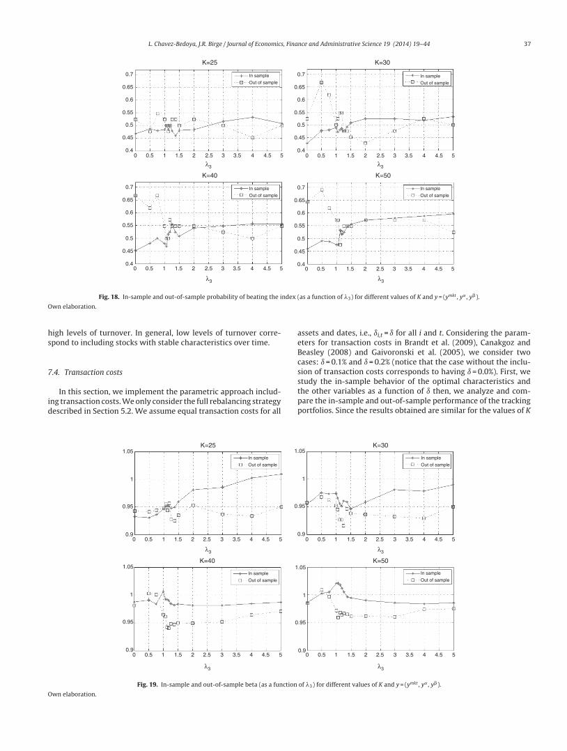
L. Chavez-Bedoya, J.R. Birge / Journal of Economics, Finance and Administrative Science 19 (2014) 19–44 37

In sample

Out of sample

In sample

Out of sample

In sample

Out of sample

In sample

Out of sample

K=25 K=30

λ3 λ3

λ3 λ3

K=40 K=50

0 0.5 1 1.5 2 2.5 3 3.5 4 4.5 5

0 0.5 1 1.5 2 2.5 3 3.5 4 4.5 5 0 0.5 1 1.5 2 2.5 3 3.5 4 4.5 5

0 0.5 1 1.5 2 2.5 3 3.5 4 4.5 5

0.7

0.65

0.6

0.55

0.5

0.45

0.4

0.7

0.65

0.6

0.55

0.5

0.45

0.4

0.7

0.65

0.6

0.55

0.5

0.45

0.4

0.7

0.65

0.6

0.55

0.5

0.45

0.4

Fig. 18. In-sample and out-of-sample probability of beating the index (as a function of �3) for different values of K and y = (ymkt , y˛ , y�).

Own elaboration.

high levels of turnover. In general, low levels of turnover corre-spond to including stocks with stable characteristics over time.

7.4. Transaction costs

In this section, we implement the parametric approach includ-ing transaction costs. We only consider the full rebalancing strategydescribed in Section 5.2. We assume equal transaction costs for all

assets and dates, i.e., ıi,t = ı for all i and t. Considering the param-eters for transaction costs in Brandt et al. (2009), Canakgoz andBeasley (2008) and Gaivoronski et al. (2005), we consider twocases: ı = 0.1% and ı = 0.2% (notice that the case without the inclu-sion of transaction costs corresponds to having ı = 0.0%). First, westudy the in-sample behavior of the optimal characteristics andthe other variables as a function of ı then, we analyze and com-pare the in-sample and out-of-sample performance of the trackingportfolios. Since the results obtained are similar for the values of K

1.05

1

0.95

0.9

1.05

1

0.95

0.9

1.05

1

0.95

0.9

1.05

1

0.95

0.90 0.5 1 1.5 2 2.5 3 3.5 4 4.5 5 0 0.5 1 1.5 2 2.5 3 3.5 4 4.5 5

0 0.5 1 1.5 2 2.5 3 3.5 4 4.5 50 0.5 1 1.5 2 2.5 3 3.5 4 4.5 5

K=25 K=30

K=40 K=50

λ3 λ3

λ3 λ3

In sample

Out of sample

In sample

Out of sample

In sample

Out of sample

In sample

Out of sample

Fig. 19. In-sample and out-of-sample beta (as a function of �3) for different values of K and y = (ymkt , y˛ , y�).

Own elaboration.

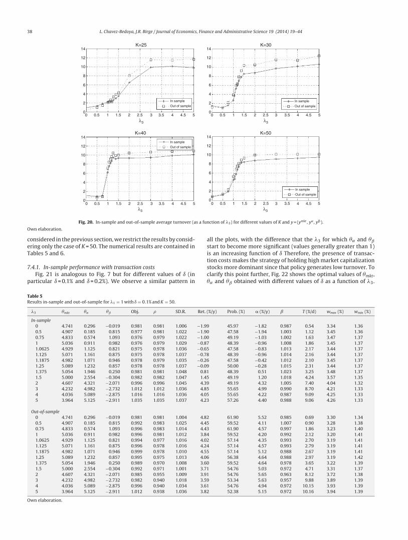
38 L. Chavez-Bedoya, J.R. Birge / Journal of Economics, Finance and Administrative Science 19 (2014) 19–44

14

12

10

8

6

4

2

0

14

12

10

8

6

4

2

0

14

12

10

8

6

4

2

0

14

12

10

8

6

4

2

0

0 0.5 1 1.5 2 2.5 3 3.5 4 4.5 5

0 0.5 1 1.5 2 2.5 3 3.5 4 4.5 5 0 0.5 1 1.5 2 2.5 3 3.5 4 4.5 5

0 0.5 1 1.5 2 2.5 3 3.5 4 4.5 5

K=25 K=30

λ3λ3

λ3λ3

K=40 K=50

In sample

Out of sample

In sample

Out of sample

In sample

Out of sample

In sample

Out of sample

Fig. 20. In-sample and out-of-sample average turnover (as a function of �3) for different values of K and y = (ymkt , y˛ , y�).

Own elaboration.

considered in the previous section, we restrict the results by consid-ering only the case of K = 50. The numerical results are contained inTables 5 and 6.

7.4.1. In-sample performance with transaction costsFig. 21 is analogous to Fig. 7 but for different values of ı (in

particular ı = 0.1% and ı = 0.2%). We observe a similar pattern in

all the plots, with the difference that the �3 for which �˛ and �ˇ

start to become more significant (values generally greater than 1)is an increasing function of ı Therefore, the presence of transac-tion costs makes the strategy of holding high market capitalizationstocks more dominant since that policy generates low turnover. Toclarify this point further, Fig. 22 shows the optimal values of �mkt,�˛ and �ˇ obtained with different values of ı as a function of �3.

Table 5Results in-sample and out-of-sample for �1 = 1 with ı = 0.1% and K = 50.

�3 �mkt �˛ �ˇ Obj. � SD.R. Ret. (%/y) Prob. (%) � (%/y) ˇ T (%/d) wmax (%) wmin (%)

In-sample0 4.741 0.296 −0.019 0.981 0.981 1.006 −1.99 45.97 −1.82 0.987 0.54 3.34 1.360.5 4.907 0.185 0.815 0.977 0.981 1.022 −1.90 47.58 −1.94 1.003 1.12 3.45 1.360.75 4.833 0.574 1.093 0.976 0.979 1.022 −1.00 49.19 −1.03 1.002 1.63 3.47 1.371 5.036 0.911 0.982 0.976 0.979 1.029 −0.87 48.39 −0.96 1.008 1.86 3.45 1.371.0625 4.929 1.125 0.821 0.975 0.978 1.036 −0.65 47.58 −0.83 1.013 2.17 3.44 1.371.125 5.071 1.161 0.875 0.975 0.978 1.037 −0.78 48.39 −0.96 1.014 2.16 3.44 1.371.1875 4.982 1.071 0.946 0.978 0.979 1.035 −0.26 47.58 −0.42 1.012 2.10 3.45 1.371.25 5.089 1.232 0.857 0.978 0.978 1.037 −0.09 50.00 −0.28 1.015 2.31 3.44 1.371.375 5.054 1.946 0.250 0.981 0.981 1.048 0.81 48.39 0.51 1.023 3.25 3.48 1.371.5 5.000 2.554 −0.304 0.982 0.982 1.047 1.45 49.19 1.20 1.018 4.24 3.57 1.352 4.607 4.321 −2.071 0.996 0.996 1.045 4.39 49.19 4.32 1.005 7.40 4.04 1.323 4.232 4.982 −2.732 1.012 1.012 1.036 4.85 55.65 4.99 0.990 8.70 4.21 1.334 4.036 5.089 −2.875 1.016 1.016 1.036 4.05 55.65 4.22 0.987 9.09 4.25 1.335 3.964 5.125 −2.911 1.035 1.035 1.037 4.23 57.26 4.40 0.988 9.06 4.26 1.33

Out-of-sample0 4.741 0.296 −0.019 0.981 0.981 1.004 4.82 61.90 5.52 0.985 0.69 3.30 1.340.5 4.907 0.185 0.815 0.992 0.983 1.025 4.45 59.52 4.11 1.007 0.90 3.28 1.380.75 4.833 0.574 1.093 0.996 0.983 1.014 4.43 61.90 4.57 0.997 1.86 3.23 1.401 5.036 0.911 0.982 0.996 0.981 1.012 3.84 59.52 4.20 0.992 2.12 3.20 1.411.0625 4.929 1.125 0.821 0.994 0.977 1.016 4.02 57.14 4.35 0.993 2.70 3.19 1.411.125 5.071 1.161 0.875 0.996 0.978 1.016 4.24 57.14 4.57 0.993 2.79 3.19 1.411.1875 4.982 1.071 0.946 0.999 0.978 1.010 4.55 57.14 5.12 0.988 2.67 3.19 1.411.25 5.089 1.232 0.857 0.995 0.975 1.013 4.06 56.38 4.64 0.988 2.97 3.19 1.421.375 5.054 1.946 0.250 0.989 0.970 1.008 3.60 59.52 4.64 0.978 3.65 3.22 1.391.5 5.000 2.554 −0.304 0.992 0.971 1.001 3.71 54.76 5.03 0.972 4.71 3.31 1.372 4.607 4.321 −2.071 0.985 0.955 1.009 3.91 54.76 5.65 0.963 8.12 3.72 1.383 4.232 4.982 −2.732 0.982 0.940 1.018 3.59 53.34 5.63 0.957 9.88 3.89 1.394 4.036 5.089 −2.875 0.996 0.940 1.034 3.61 54.76 4.94 0.972 10.15 3.93 1.395 3.964 5.125 −2.911 1.012 0.938 1.036 3.82 52.38 5.15 0.972 10.16 3.94 1.39

Own elaboration.

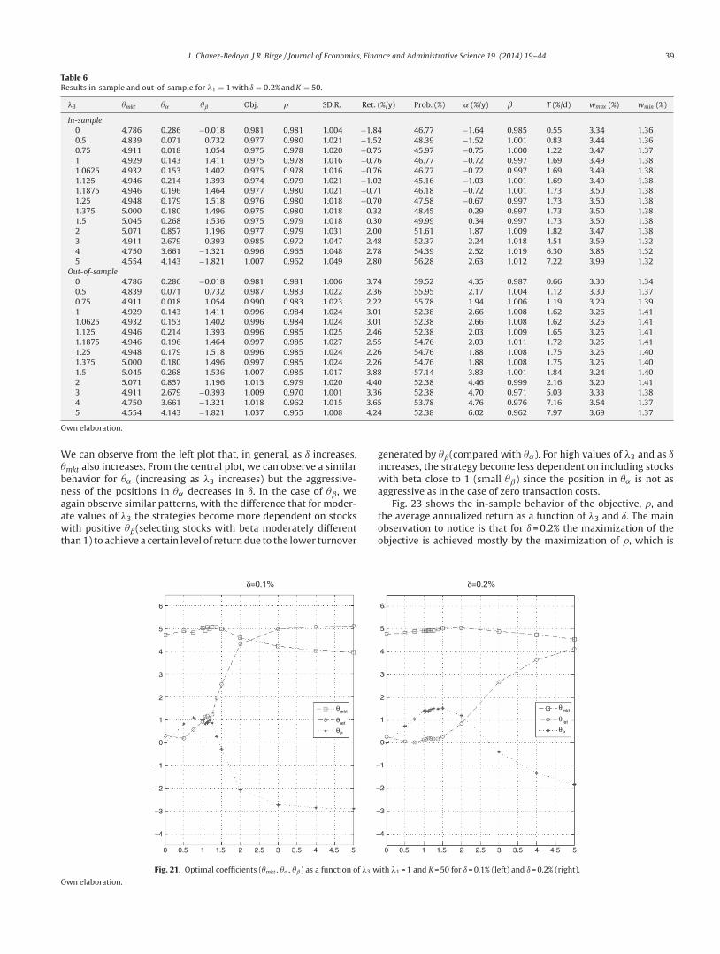
L. Chavez-Bedoya, J.R. Birge / Journal of Economics, Finance and Administrative Science 19 (2014) 19–44 39

Table 6Results in-sample and out-of-sample for �1 = 1 with ı = 0.2% and K = 50.

�3 �mkt �˛ �ˇ Obj. � SD.R. Ret. (%/y) Prob. (%) ˛ (%/y) ˇ T (%/d) wmax (%) wmin (%)

In-sample0 4.786 0.286 −0.018 0.981 0.981 1.004 −1.84 46.77 −1.64 0.985 0.55 3.34 1.360.5 4.839 0.071 0.732 0.977 0.980 1.021 −1.52 48.39 −1.52 1.001 0.83 3.44 1.360.75 4.911 0.018 1.054 0.975 0.978 1.020 −0.75 45.97 −0.75 1.000 1.22 3.47 1.371 4.929 0.143 1.411 0.975 0.978 1.016 −0.76 46.77 −0.72 0.997 1.69 3.49 1.381.0625 4.932 0.153 1.402 0.975 0.978 1.016 −0.76 46.77 −0.72 0.997 1.69 3.49 1.381.125 4.946 0.214 1.393 0.974 0.979 1.021 −1.02 45.16 −1.03 1.001 1.69 3.49 1.381.1875 4.946 0.196 1.464 0.977 0.980 1.021 −0.71 46.18 −0.72 1.001 1.73 3.50 1.381.25 4.948 0.179 1.518 0.976 0.980 1.018 −0.70 47.58 −0.67 0.997 1.73 3.50 1.381.375 5.000 0.180 1.496 0.975 0.980 1.018 −0.32 48.45 −0.29 0.997 1.73 3.50 1.381.5 5.045 0.268 1.536 0.975 0.979 1.018 0.30 49.99 0.34 0.997 1.73 3.50 1.382 5.071 0.857 1.196 0.977 0.979 1.031 2.00 51.61 1.87 1.009 1.82 3.47 1.383 4.911 2.679 −0.393 0.985 0.972 1.047 2.48 52.37 2.24 1.018 4.51 3.59 1.324 4.750 3.661 −1.321 0.996 0.965 1.048 2.78 54.39 2.52 1.019 6.30 3.85 1.325 4.554 4.143 −1.821 1.007 0.962 1.049 2.80 56.28 2.63 1.012 7.22 3.99 1.32

Out-of-sample0 4.786 0.286 −0.018 0.981 0.981 1.006 3.74 59.52 4.35 0.987 0.66 3.30 1.340.5 4.839 0.071 0.732 0.987 0.983 1.022 2.36 55.95 2.17 1.004 1.12 3.30 1.370.75 4.911 0.018 1.054 0.990 0.983 1.023 2.22 55.78 1.94 1.006 1.19 3.29 1.391 4.929 0.143 1.411 0.996 0.984 1.024 3.01 52.38 2.66 1.008 1.62 3.26 1.411.0625 4.932 0.153 1.402 0.996 0.984 1.024 3.01 52.38 2.66 1.008 1.62 3.26 1.411.125 4.946 0.214 1.393 0.996 0.985 1.025 2.46 52.38 2.03 1.009 1.65 3.25 1.411.1875 4.946 0.196 1.464 0.997 0.985 1.027 2.55 54.76 2.03 1.011 1.72 3.25 1.411.25 4.948 0.179 1.518 0.996 0.985 1.024 2.26 54.76 1.88 1.008 1.75 3.25 1.401.375 5.000 0.180 1.496 0.997 0.985 1.024 2.26 54.76 1.88 1.008 1.75 3.25 1.401.5 5.045 0.268 1.536 1.007 0.985 1.017 3.88 57.14 3.83 1.001 1.84 3.24 1.402 5.071 0.857 1.196 1.013 0.979 1.020 4.40 52.38 4.46 0.999 2.16 3.20 1.413 4.911 2.679 −0.393 1.009 0.970 1.001 3.36 52.38 4.70 0.971 5.03 3.33 1.384 4.750 3.661 −1.321 1.018 0.962 1.015 3.65 53.78 4.76 0.976 7.16 3.54 1.375 4.554 4.143 −1.821 1.037 0.955 1.008 4.24 52.38 6.02 0.962 7.97 3.69 1.37

Own elaboration.

We can observe from the left plot that, in general, as ı increases,�mkt also increases. From the central plot, we can observe a similarbehavior for �˛ (increasing as �3 increases) but the aggressive-ness of the positions in �˛ decreases in ı. In the case of �ˇ, weagain observe similar patterns, with the difference that for moder-ate values of �3 the strategies become more dependent on stockswith positive �ˇ(selecting stocks with beta moderately differentthan 1) to achieve a certain level of return due to the lower turnover

generated by �ˇ(compared with �˛). For high values of �3 and as ıincreases, the strategy become less dependent on including stockswith beta close to 1 (small �ˇ) since the position in �˛ is not asaggressive as in the case of zero transaction costs.

Fig. 23 shows the in-sample behavior of the objective, �, andthe average annualized return as a function of �3 and ı. The mainobservation to notice is that for ı = 0.2% the maximization of theobjective is achieved mostly by the maximization of �, which is

6

5

4

3

2

1

0

–1

–2

–3

–4

6

5

4

3

2

1

0

–1

–2

–3

–4

0 0.5 1 1.5 2 2.5 3 3.5 4 4.5 5 0 0.5 1 1.5 2 2.5 3 3.5 4 4.5 5

δ=0.1%

θmkt

θret

θP

θmkt

θret

θP

δ=0.2%

Fig. 21. Optimal coefficients (�mkt , �˛ , �ˇ) as a function of �3 with �1 = 1 and K = 50 for ı = 0.1% (left) and ı = 0.2% (right).

Own elaboration.

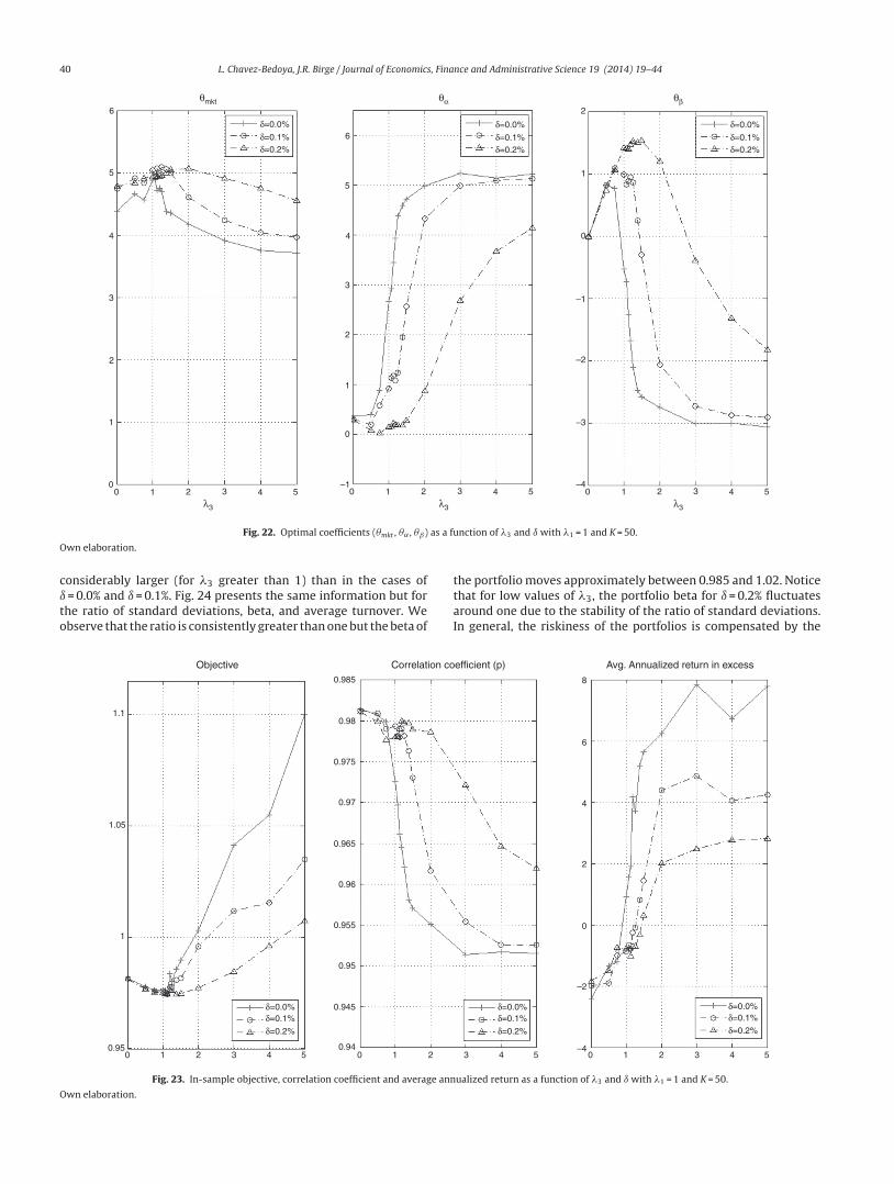
40 L. Chavez-Bedoya, J.R. Birge / Journal of Economics, Finance and Administrative Science 19 (2014) 19–44

5

4

3

2

1

00 1 2 3 4 5 0 1 2 3 4 5 0 1 2 3 4 5

6

5

3

4

2

1

0

–1

6

2

1

0

–1

–2

–3

–4

θmkt

δ=0.0%

δ=0.1%δ=0.2%

δ=0.0%

δ=0.1%δ=0.2%

δ=0.0%

δ=0.1%δ=0.2%

θα θβ

λ3 λ3 λ3

Fig. 22. Optimal coefficients (�mkt , �˛ , �ˇ) as a function of �3 and ı with �1 = 1 and K = 50.

Own elaboration.

considerably larger (for �3 greater than 1) than in the cases ofı = 0.0% and ı = 0.1%. Fig. 24 presents the same information but forthe ratio of standard deviations, beta, and average turnover. Weobserve that the ratio is consistently greater than one but the beta of

the portfolio moves approximately between 0.985 and 1.02. Noticethat for low values of �3, the portfolio beta for ı = 0.2% fluctuatesaround one due to the stability of the ratio of standard deviations.In general, the riskiness of the portfolios is compensated by the

1.1

0.985 8

6

4

2

0

–2

–4

0.98

0.975

0.97

0.965

0.96

0.955

0.95

0.945

0.94

1.05

1

0.950 1 2 3 4 5 0 1 2 3 4 5 0 1 2 3 4 5

Objective Correlation coefficient (p) Avg. Annualized return in excess

δ=0.0%δ=0.1%

δ=0.2%

δ=0.0%δ=0.1%

δ=0.2%

δ=0.0%δ=0.1%

δ=0.2%

Fig. 23. In-sample objective, correlation coefficient and average annualized return as a function of �3 and ı with �1 = 1 and K = 50.

Own elaboration.

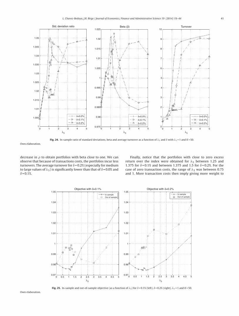
L. Chavez-Bedoya, J.R. Birge / Journal of Economics, Finance and Administrative Science 19 (2014) 19–44 41

1.05

1.025 10

9

8

7

6

5

4

3

2

1

0

1.02

1.015

1.01

1.005

0.995

0.99

0.985

0.98

0.975

1

1.045

1.04

1.035

1.03

1.025

1.02

1.015

1.01

1.005

10 1 2

λ3 λ3 λ3

3 4 5 0 1 2 3 4 5 0 1 2 3 4 5

Std. deviation ratio Beta (β) Turnover

δ=0.0%

δ=0.1%

δ=0.2%

δ=0.0%

δ=0.1%

δ=0.2%

δ=0.0%

δ=0.1%

δ=0.2%

Fig. 24. In-sample ratio of standard deviations, beta and average turnover as a function of �3 and ı with �1 = 1 and K = 50.

Own elaboration.

decrease in � to obtain portfolios with beta close to one. We canobserve that because of transactions costs, the portfolios incur lessturnovers. The average turnover for ı = 0.2% (especially for mediumto large values of �3) is significantly lower than that of ı = 0.0% andı = 0.1%.

Finally, notice that the portfolios with close to zero excessreturn over the index were obtained for �3 between 1.25 and1.375 for ı = 0.1% and between 1.375 and 1.5 for ı = 0.2%. For thecase of zero transaction costs, the range of �3 was between 0.75and 1. More transaction costs then imply giving more weight to

1.05

1.04

1.03

1.02

1.01

1

0.99

0.98

0.97

1.05

1.04

1.03

1.02

1.01

1

0.99

0.98

0.970 0.5 1 1.5 2 2.5 3 3.5 4 4.5 5 0 0.5 1 1.5 2 2.5 3 3.5 4 4.5 5

Objective with δ=0.1% Objective with δ=0.2%

In sampleOut of sample

In sampleOut of sample

λ3 λ3

Fig. 25. In-sample and out-of-sample objective (as a function of �3) for ı = 0.1% (left), ı = 0.2% (right), �1 = 1 and K = 50.

Own elaboration.

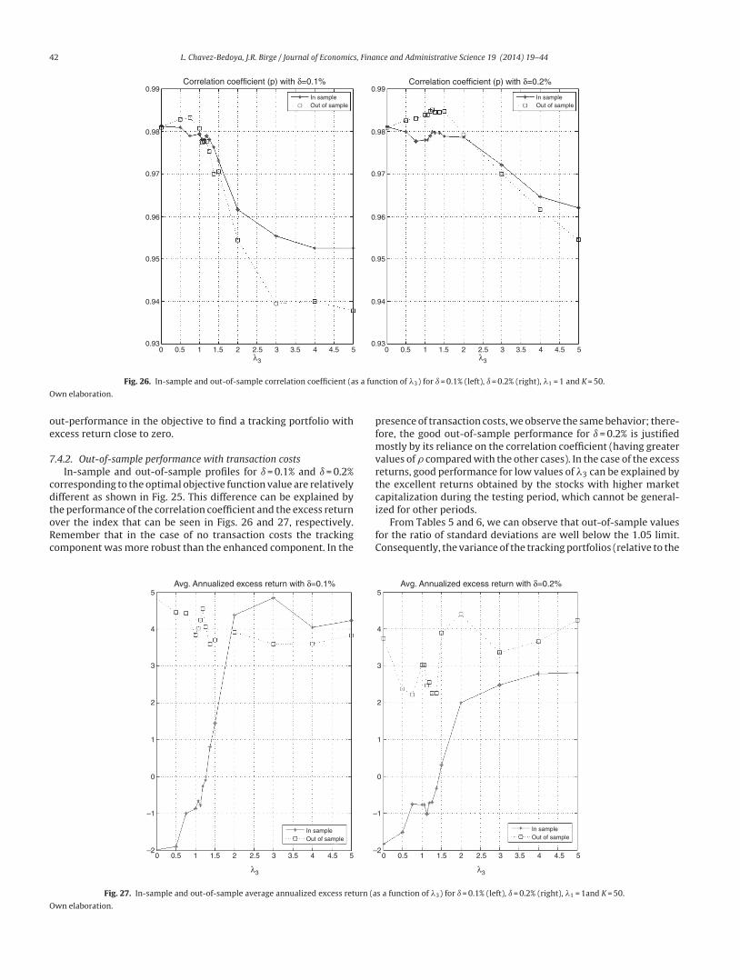
42 L. Chavez-Bedoya, J.R. Birge / Journal of Economics, Finance and Administrative Science 19 (2014) 19–44

0.93

0.94

0.95

0.96

0.97

0.98

0.99

0 0.5 1 1.5 2 2.5 3 3.5 4 4.5 5

Correlation coefficient (p) with δ=0.1%

In sampleOut of sample

λ3

0.93

0.94

0.95

0.96

0.97

0.98

0.99

0 0.5 1 1.5 2 2.5 3 3.5 4 4.5 5

Correlation coefficient (p) with δ=0.2%

In sampleOut of sample

λ3

Fig. 26. In-sample and out-of-sample correlation coefficient (as a function of �3) for ı = 0.1% (left), ı = 0.2% (right), �1 = 1 and K = 50.

Own elaboration.

out-performance in the objective to find a tracking portfolio withexcess return close to zero.

7.4.2. Out-of-sample performance with transaction costsIn-sample and out-of-sample profiles for ı = 0.1% and ı = 0.2%

corresponding to the optimal objective function value are relativelydifferent as shown in Fig. 25. This difference can be explained bythe performance of the correlation coefficient and the excess returnover the index that can be seen in Figs. 26 and 27, respectively.Remember that in the case of no transaction costs the trackingcomponent was more robust than the enhanced component. In the

presence of transaction costs, we observe the same behavior; there-fore, the good out-of-sample performance for ı = 0.2% is justifiedmostly by its reliance on the correlation coefficient (having greatervalues of � compared with the other cases). In the case of the excessreturns, good performance for low values of �3 can be explained bythe excellent returns obtained by the stocks with higher marketcapitalization during the testing period, which cannot be general-ized for other periods.

From Tables 5 and 6, we can observe that out-of-sample valuesfor the ratio of standard deviations are well below the 1.05 limit.Consequently, the variance of the tracking portfolios (relative to the

5

4

3

2

1

0

–1

–2

5

4

3

2

1

0

–1

–20 0.5 1 1.5 2 2.5 3 3.5 4 4.5 5 0 0.5 1 1.5 2 2.5 3 3.5 4 4.5 5

Avg. Annualized excess return with δ=0.1% Avg. Annualized excess return with δ=0.2%

In sampleOut of sample

In sampleOut of sample

λ3 λ3

Fig. 27. In-sample and out-of-sample average annualized excess return (as a function of �3) for ı = 0.1% (left), ı = 0.2% (right), �1 = 1and K = 50.

Own elaboration.

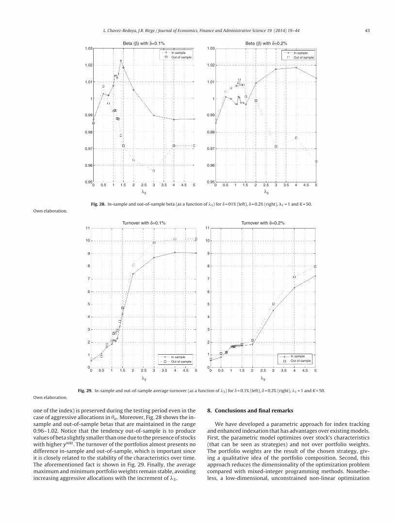
L. Chavez-Bedoya, J.R. Birge / Journal of Economics, Finance and Administrative Science 19 (2014) 19–44 43

1.03

1.02

1.01

1

0.99

0.98

0.97

0.96

0.95

1.03

1.02

1.01

1

0.99

0.98

0.97

0.96

0.950 0.5 1 1.5 2 2.5 3 3.5 4 4.5 5 0 0.5 1 1.5 2 2.5 3 3.5 4 4.5 5

In sampleOut of sample

In sampleOut of sample

Beta (β) with δ=0.2%Beta (β) with δ=0.1%

λ3 λ3

Fig. 28. In-sample and out-of-sample beta (as a function of �3) for ı = 01% (left), ı = 0.2% (right), �1 = 1 and K = 50.

Own elaboration.

11

10

9

8

7

6

5

4

3

2

1

00 0.5 1 1.5 2 2.5 3

λ3 λ3

3.5 4 4.5 5 00

11

10

9

8

7

6

5

4

3

2

1

0.5 1 1.5 2 2.5 3 3.5 4 4.5 5

In sampleOut of sample

In sampleOut of sample

Turnover with δ=0.1% Turnover with δ=0.2%

Fig. 29. In-sample and out-of-sample average turnover (as a function of �3) for ı = 0.1% (left), ı = 0.2% (right), �1 = 1 and K = 50.

Own elaboration.

one of the index) is preserved during the testing period even in thecase of aggressive allocations in �˛. Moreover, Fig. 28 shows the in-sample and out-of-sample betas that are maintained in the range0.96–1.02. Notice that the tendency out-of-sample is to producevalues of beta slightly smaller than one due to the presence of stockswith higher ymkt. The turnover of the portfolios almost presents nodifference in-sample and out-of-sample, which is important sinceit is closely related to the stability of the characteristics over time.The aforementioned fact is shown in Fig. 29. Finally, the averagemaximum and minimum portfolio weights remain stable, avoidingincreasing aggressive allocations with the increment of �3.

8. Conclusions and final remarks

We have developed a parametric approach for index trackingand enhanced indexation that has advantages over existing models.First, the parametric model optimizes over stock’s characteristics(that can be seen as strategies) and not over portfolio weights.The portfolio weights are the result of the chosen strategy, giv-ing a qualitative idea of the portfolio composition. Second, thisapproach reduces the dimensionality of the optimization problemcompared with mixed-integer programming methods. Nonethe-less, a low-dimensional, unconstrained non-linear optimization

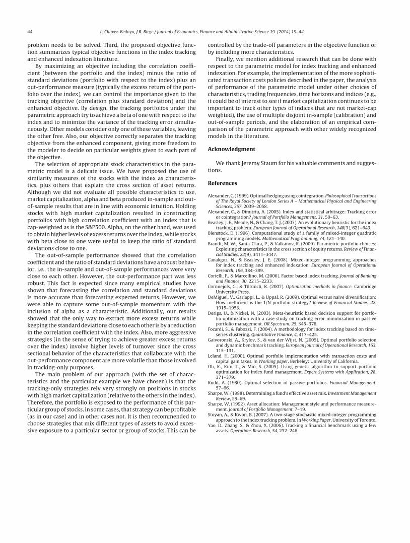
44 L. Chavez-Bedoya, J.R. Birge / Journal of Economics, Finance and Administrative Science 19 (2014) 19–44

problem needs to be solved. Third, the proposed objective func-tion summarizes typical objective functions in the index trackingand enhanced indexation literature.

By maximizing an objective including the correlation coeffi-cient (between the portfolio and the index) minus the ratio ofstandard deviations (portfolio with respect to the index) plus anout-performance measure (typically the excess return of the port-folio over the index), we can control the importance given to thetracking objective (correlation plus standard deviation) and theenhanced objective. By design, the tracking portfolios under theparametric approach try to achieve a beta of one with respect to theindex and to minimize the variance of the tracking error simulta-neously. Other models consider only one of these variables, leavingthe other free. Also, our objective correctly separates the trackingobjective from the enhanced component, giving more freedom tothe modeler to decide on particular weights given to each part ofthe objective.

The selection of appropriate stock characteristics in the para-metric model is a delicate issue. We have proposed the use ofsimilarity measures of the stocks with the index as characteris-tics, plus others that explain the cross section of asset returns.Although we did not evaluate all possible characteristics to use,market capitalization, alpha and beta produced in-sample and out-of-sample results that are in line with economic intuition. Holdingstocks with high market capitalization resulted in constructingportfolios with high correlation coefficient with an index that iscap-weighted as is the S&P500. Alpha, on the other hand, was usedto obtain higher levels of excess returns over the index, while stockswith beta close to one were useful to keep the ratio of standarddeviations close to one.

The out-of-sample performance showed that the correlationcoefficient and the ratio of standard deviations have a robust behav-ior, i.e., the in-sample and out-of-sample performances were veryclose to each other. However, the out-performance part was lessrobust. This fact is expected since many empirical studies haveshown that forecasting the correlation and standard deviationsis more accurate than forecasting expected returns. However, wewere able to capture some out-of-sample momentum with theinclusion of alpha as a characteristic. Additionally, our resultsshowed that the only way to extract more excess returns whilekeeping the standard deviations close to each other is by a reductionin the correlation coefficient with the index. Also, more aggressivestrategies (in the sense of trying to achieve greater excess returnsover the index) involve higher levels of turnover since the crosssectional behavior of the characteristics that collaborate with theout-performance component are more volatile than those involvedin tracking-only purposes.

The main problem of our approach (with the set of charac-teristics and the particular example we have chosen) is that thetracking-only strategies rely very strongly on positions in stockswith high market capitalization (relative to the others in the index).Therefore, the portfolio is exposed to the performance of this par-ticular group of stocks. In some cases, that strategy can be profitable(as in our case) and in other cases not. It is then recommended tochoose strategies that mix different types of assets to avoid exces-sive exposure to a particular sector or group of stocks. This can be

controlled by the trade-off parameters in the objective function orby including more characteristics.

Finally, we mention additional research that can be done withrespect to the parametric model for index tracking and enhancedindexation. For example, the implementation of the more sophisti-cated transaction costs policies described in the paper, the analysisof performance of the parametric model under other choices ofcharacteristics, trading frequencies, time horizons and indices (e.g.,it could be of interest to see if market capitalization continues to beimportant to track other types of indices that are not market-capweighted), the use of multiple disjoint in-sample (calibration) andout-of-sample periods, and the elaboration of an empirical com-parison of the parametric approach with other widely recognizedmodels in the literature.

Acknowledgment

We thank Jeremy Staum for his valuable comments and sugges-tions.

References

Alexander, C. (1999). Optimal hedging using cointegration. Philosophical Transactionsof The Royal Society of London Series A – Mathematical Physical and EngineeringSciences, 357, 2039–2058.

Alexander, C., & Dimitriu, A. (2005). Index and statistical arbitrage: Tracking erroror cointegration? Journal of Portfolio Management, 31, 50–63.

Beasley, J. E., Meade, N., & Chang, T. J. (2003). An evolutionary heuristic for the indextracking problem. European Journal of Operational Research, 148(3), 621–643.

Bienstock, D. (1996). Computational study of a family of mixed-integer quadraticprogramming models. Mathematical Programming, 74, 121–140.

Brandt, M. W., Santa-Clara, P., & Valkanov, R. (2009). Parametric portfolio choices:Exploiting characteristics in the cross section of equity returns. Review of Finan-cial Studies, 22(9), 3411–3447.

Canakgoz, N., & Beasley, J. E. (2008). Mixed-integer programming approachesfor index tracking and enhanced indexation. European Journal of OperationalResearch, 196, 384–399.

Corielli, F., & Marcellino, M. (2006). Factor based index tracking. Journal of Bankingand Finance, 30, 2215–2233.

Cornuejols, G., & Tütüncü, R. (2007). Optimization methods in finance. CambridgeUniversity Press.

DeMiguel, V., Garlappi, L., & Uppal, R. (2009). Optimal versus naive diversification:How inefficient is the 1/N portfolio strategy? Review of Financial Studies, 22,1915–1953.

Derigs, U., & Nickel, N. (2003). Meta-heuristic based decision support for portfo-lio optimization with a case study on tracking error minimization in passiveportfolio management. OR Spectrum, 25, 345–378.

Focardi, S., & Fabozzi, F. (2004). A methodology for index tracking based on time-series clustering. Quantitative Finance, 4, 417–425.

Gaivoronski, A., Krylov, S., & van der Wijst, N. (2005). Optimal portfolio selectionand dynamic benchmark tracking. European Journal of Operational Research, 163,115–131.

Leland, H. (2000). Optimal portfolio implementation with transaction costs andcapital gain taxes. In Working paper. Berkeley: University of California.

Oh, K., Kim, T., & Min, S. (2005). Using genetic algorithm to support portfoliooptimization for index fund management. Expert Systems with Application, 28,371–379.

Rudd, A. (1980). Optimal selection of passive portfolios. Financial Management,57–66.

Sharpe, W. (1988). Determining a fund’s effective asset mix. Investment ManagementReview, 59–69.

Sharpe, W. (1992). Asset allocation: Management style and performance measure-ment. Journal of Portfolio Management, 7–19.

Stoyan, A., & Kwon, B. (2007). A two-stage stochastic mixed-integer programmingapproach to the index tracking problem. In Working Paper. University of Toronto.

Yao, D., Zhang, S., & Zhou, X. (2006). Tracking a financial benchmark using a fewassets. Operations Research, 54, 232–246.