


Languages
Pages
Legal


1
LECTURE NOTES
ON
COMPUTER NETWORKS
IV B. Tech I semester
Mr. P. Ravinder
Associate Professor
ELECTRONICS AND COMMUNICATION ENGINEERING
INSTITUTE OF AERONAUTICAL ENGINEERING
(Autonomous) DUNDIGAL, HYDERABAD - 500 043

2
UNIT-I
Overview of the Internet, Physical Layer and Data Link Layer
A network is the interconnection of a set of devices capable of communication. In this definition,
a device can be a host (or an end system as it is sometimes called) such as a large computer,
desktop, laptop, workstation, cellular phone, or security system. A device in this definition can
also be a connecting device such as a router, which connects the network to other networks, a
switch, which connects devices together, a modem (modulator-demodulator), which changes the
form of data, and so on. These devices in a network are connected using wired or wireless
transmission media such as cable or air. When we connect two computers at home using a plug-
and-play router, we have created a network, although very small.
Network Criteria A network must be able to meet a certain number of criteria. The most important of these are
performance, reliability, and security.
Performance Performance can be measured in many ways, including transit time and response time. Transit
time is the amount of time required for a message to travel from one device to another. Response
time is the elapsed time between an inquiry and a response. The performance of a network
depends on a number of factors, including the number of users, the type of transmission medium,
the capabilities of the connected hardware, and the efficiency of the software. Performance is
often evaluated by two networking metrics: throughput and delay. We often need more
throughputs and less delay. However, these two criteria are often contradictory. If we try to send
more data to the network, we may increase throughput but we increase the delay because of
traffic congestion in the network.
Reliability In addition to accuracy of delivery, network reliability is measured by the frequency of failure,
the time it takes a link to recover from a failure, and the network's robustness in a catastrophe.
Security Network security issues include protecting data from unauthorized access, protecting data from
damage and development, and implementing policies and procedures for recovery from breaches and data losses.
Physical Structures Before discussing networks, we need to define some network attributes.
Type of Connection A network is two or more devices connected through links. A link is a communications pathway
that transfers data from one device to another. For visualization purposes, it is simplest to
imagine any link as a line drawn between two points. For communication to occur, two devices must be connected in some way to the same link at the same time. There are two possible types
of connections: point-to-point and multipoint.

3
Point-to-Point A point-to-point connection provides a dedicated link between two devices. The entire capacity
of the link is reserved for transmission between those two devices. Most point-to-point
connections use an actual length of wire or cable to connect the two ends, but other options, such
as microwave or satellite links, are also possible. When we change television channels by
infrared remote control, we are establishing a point-to-point connection between the remote
control and the television's control system.
Multipoint A multipoint (also called multidrop) connection is one in which more than two specific devices share a single link.
In a multipoint environment, the capacity of the channel is shared, either spatially or temporally.
If several devices can use the link simultaneously, it is a spatially shared connection. If users
must take turns, it is a timeshared connection.
PROTOCOL LAYERING We defined the term protocol in Chapter 1. In data communication and networking, a protocol
defines the rules that both the sender and receiver and all intermediate devices need to follow to
be able to communicate effectively. When communication is simple, we may need only one
simple protocol; when the communication is complex, we may need to divide the task between different layers, in which case we need a protocol at each layer, or protocol layering.
Scenarios
Let us develop two simple scenarios to better understand the need for protocol layering.
First Scenario In the first scenario, communication is so simple that it can occur in only one layer. Assume Maria and Ann are neighbors with a lot of common ideas. Communication between Maria and
Ann takes place in one layer, face to face, in the same language, as shown in Figure.

4
Even in this simple scenario, we can see that a set of rules needs to be followed. First, Maria and
Ann know that they should greet each other when they meet. Second, they know that they should
confine their vocabulary to the level of their friendship. Third, each party knows that she should
refrain from speaking when the other party is speaking. Fourth, each party knows that the
conversation should be a dialog, not a monolog: both should have the opportunity to talk about
the issue. Fifth, they should exchange some nice words when they leave. We can see that the
protocol used by Maria and Ann is different from the communication between a professor and
the students in a lecture hall. The communication in the second case is mostly monolog; the
professor talks most of the time unless a student has a question, a situation in which the protocol
dictates that she should raise her hand and wait for permission to speak. In this case, the
communication is normally very formal and limited to the subject being taught.
Second Scenario In the second scenario, we assume that Ann is offered a higher-level position in her company, but
needs to move to another branch located in a city very far from Maria. The two friends still want
to continue their communication and exchange ideas because they have come up with an
innovative project to start a new business when they both retire. They decide to continue their
conversation using regular mail through the post office. However, they do not want their ideas to
be revealed by other people if the letters are intercepted. They agree on an encryption/decryption
technique. The sender of the letter encrypts it to make it unreadable by an intruder; the receiver
of the letter decrypts it to get the original letter. We discuss the encryption/decryption methods in
Chapter 31, but for the moment we assume that Maria and Ann use one technique that makes it
hard to decrypt the letter if one does not have the key for doing so. Now we can say that the
communication between Maria and Ann takes place in three layers, as shown in Figure. We
assume that Ann and Maria each have three machines (or robots) that can perform the task at
each layer.

5
Principles of Protocol Layering
Let us discuss two principles of protocol layering.
First Principle The first principle dictates that if we want bidirectional communication, we need to make each
layer so that it is able to perform two opposite tasks, one in each direction. For example, the third layer task is to listen (in one direction) and talk (in the other direction). The second layer needs
to be able to encrypt and decrypt. The first layer needs to send and receive mail.
Second Principle The second principle that we need to follow in protocol layering is that the two objects under
each layer at both sites should be identical. For example, the object under layer 3 at both sites should be a plaintext letter. both sites should be a cipher text letter. The object under layer 1 at
both sites should be a piece of mail.
Logical Connections After following the above two principles, we can think about logical connection between each
layer as shown in below figure. This means that we have layer-to-layer communication. Maria
and Ann can think that there is a logical (imaginary) connection at each layer through which they
can send the object created from that layer. We will see that the concept of logical connection
will help us better understand the task of layering. We encounter in data communication and
networking.

6
TCP/IP PROTOCOL SUITE Now that we know about the concept of protocol layering and the logical communication
between layers in our second scenario, we can introduce the TCP/IP (Transmission Control
Protocol/Internet Protocol). TCP/IP is a protocol suite (a set of protocols organized in different
layers) used in the Internet today. It is a hierarchical protocol made up of interactive modules,
each of which provides a specific functionality. The term hierarchical means that each upper
level protocol is supported by the services provided by one or more lower level protocols. The
original TCP/IP protocol suite was defined as four software layers built upon the hardware.
Today, however, TCP/IP is thought of as a five-layer model. Following figure shows both
configurations.
Layered Architecture To show how the layers in the TCP/IP protocol suite are involved in communication between
two hosts, we assume that we want to use the suite in a small internet made up of three LANs
(links), each with a link-layer switch. We also assume that the links are connected by one router,
as shown in below Figure.

7
Layers in the TCP/IP Protocol Suite After the above introduction, we briefly discuss the functions and duties of layers in the TCP/IP
protocol suite. Each layer is discussed in detail in the next five parts of the book. To better
understand the duties of each layer, we need to think about the logical connections between
layers. Below figure shows logical connections in our simple internet.
Using logical connections makes it easier for us to think about the duty of each layer. As the figure shows, the duty of the application, transport, and network layers is end-to-end. However,
the duty of the data-link and physical layers is hop-to-hop, in which a hop is a host or router. In

8
other words, the domain of duty of the top three layers is the internet, and the domain of duty of
the two lower layers is the link. Another way of thinking of the logical connections is to think
about the data unit created from each layer. In the top three layers, the data unit (packets) should
not be changed by any router or link-layer switch. In the bottom two layers, the packet created by
the host is changed only by the routers, not by the link-layer switches. Below figure shows the
second principle discussed previously for protocol layering. We show the identical objects below
each layer related to each device.
Note that, although the logical connection at the network layer is between the two hosts, we can only say that identical objects exist between two hops in this case because a router may fragment
the packet at the network layer and send more packets than received (see fragmentation in
Chapter 19). Note that the link between two hops does not change the object.
Description of Each Layer After understanding the concept of logical communication, we are ready to briefly discuss the duty of each layer.
Physical Layer We can say that the physical layer is responsible for carrying individual bits in a frame across the
link. Although the physical layer is the lowest level in the TCPIIP protocol suite, the
communication between two devices at the physical layer is still a logical communication
because there is another, hidden layer, the transmission media, under the physical layer. Two
devices are connected by a transmission medium (cable or air). We need to know that the
transmission medium does not carry bits; it carries electrical or optical signals. So the bits
received in a frame from the data-link layer are transformed and sent through the transmission
media, but we can think that the logical unit between two physical layers in two devices is a bit.
There are several protocols that transform a bit to a signal.
Data-link Layer We have seen that an internet is made up of several links (LANs and WANs) connected by routers. There may be several overlapping sets of links that a datagram can travel from the host

9
to the destination. The routers are responsible for choosing the best links. However, when the
next link to travel is determined by the router, the data-link layer is responsible for taking the
datagram and moving it across the link. The link can be a wired LAN with a link-layer switch, a
wireless LAN, a wired WAN, or a wireless WAN. We can also have different protocols used
with any link type. In each case, the data-link layer is responsible for moving the packet through
the link. TCP/IP does not define any specific protocol for the data-link layer. It supports all the standard and proprietary protocols. Any protocol that can take the datagram and carry it
through the link suffices for the network layer. The data-link layer takes a datagram and
encapsulates it in a packet called «frame. Each link-layer protocol may provide a different service. Some link-layer protocols provide complete error detection and correction, some provide
only error correction.
Network Layer The network layer is responsible for creating a connection between the source computer and the
destination computer. The communication at the network layer is host-to-host. However, since
there can be several routers from the source to the destination, the routers in the path are
responsible for choosing the best route for each packet. We can say that the network layer is
responsible for host-to-host communication and routing the packet through possible routes.
Again, we may ask ourselves why we need the network layer. We could have added the routing
duty to the transport layer and dropped this layer. One reason, as we said before, is the separation
of different tasks between different layers. The second reason is that the routers do not need the
application and transport layers.
Transport Layer The logical connection at the transport layer is also end-to-end. The transport layer at the source
host gets the message from the application layer, encapsulates it in a transport layer packet
(called a segment or a user datagram in different protocols) and sends it, through the logical
(imaginary) connection, to the transport layer at the destination host. In other words, the transport
layer is responsible for giving services to the application layer: to get a message from an
application program running on the source host and deliver it to the corresponding application
program on the destination host. We may ask why we need an end-to-end transport layer when
we already have an end-to-end application layer. The reason is the separation of tasks and duties,
which we discussed earlier. The transport layer should be independent of the application layer. In
addition, we will see that we have more than one protocol in the transport layer, which means
that each application program can use the protocol that best matches its requirement. Application Layer The logical connection between the two application layers is end to-end. The two application
layers exchange messages between each other as though there were a bridge between the two
layers. However, we should know that the communication is done through all the layers.
Communication at the application layer is between two processes (two programs running at this
layer). To communicate, a process sends a request to the other process and receives a response.
Process-to-process communication is the duty of the application layer. The application layer in
the Internet includes many predefined protocols, but a user can also create a pair of processes to
be run at the two hosts.

10
THE OSI MODEL Although, when speaking of the Internet, everyone talks about the TCP/IP protocol suite, this
suite is not the only suite of protocols defined. Established in 1947, the International
Organization for Standardization (ISO) is a multinational body dedicated to worldwide
agreement on international standards. Almost three-fourths of the countries in the world are
represented in the ISO. An ISO standard that covers all aspects of network communications is the
Open Systems Interconnection (OSI) model. It was first introduced in the late 1970s. ISO is the organization; OSI is the model The OSI model is a layered framework for the design of network systems that allows
communication between all types of computer systems. It consists of seven separate but related layers, each of which defines a part of the process of moving information across a network
INTERNET HISTORY Now that we have given an overview of the Internet, let us give a brief history of the internet. This brief history makes it clear how the Internet has evolved from a private network to a
global one in less than 40 years.
Early History There were some communication networks, such as telegraph and telephone networks, before
1960. These networks were suitable for constant-rate communication at that time, which means
that after a connection was made between two users, the encoded message (telegraphy) or voice (telephony) could be exchanged.
ARPANET In the mid-1960s, mainframe computers in research organizations were stand-alone devices.
Computers from different manufacturers were unable to communicate with one another. The
Advanced Research Projects Agency (ARPA) in the Department of Defense (DOD) was
interested in finding a way to connect computers so that the researchers they funded could share
their findings, thereby reducing costs and eliminating duplication of effort. In 1967, at an
Association for Computing Machinery (ACM) meeting, ARPA presented its ideas for the

11
Advanced Research Projects Agency Network (ARPANET), a small network of connected
computers. The idea was that each host computer (not necessarily from the same manufacturer)
would be attached to a specialized computer, called an interface message processor (IMP). The
IMPs, in turn, would be connected to each other. Each IMP had to be able to communicate with other IMPs as well as with its own attached host.
Birth of the Internet In 1972, Vint Cerf and Bob Kahn, both of whom were part of the core ARPANET group,
collaborated on what they called the Internetting Project. TCPI/P Cerf and Kahn's landmark
1973 paper outlined the protocols to achieve end-to-end delivery of data. This was a new version
of NCP. This paper on transmission control protocol (TCP) included concepts such as
encapsulation, the datagram, and the functions of a gateway. Transmission Control Protocol
(TCP) and Internet Protocol (IP). IP would handle datagram routing while TCP would be
responsible for higher level functions such as segmentation, reassembly, and error detection. The
new combination became known as TCPIIP.
MILNET In 1983, ARPANET split into two networks: Military Network (MILNET) for military users and ARPANET for nonmilitary users.
CSNET Another milestone in Internet history was the creation of CSNET in 1981. Computer Science Network (CSNET) was a network sponsored by the National Science Foundation (NSF).
NSFNET With the success of CSNET, the NSF in 1986 sponsored the National Science Foundation
Network (NSFNET), a backbone that connected five supercomputer centers located throughout the United States.
ANSNET In 1991, the U.S. government decided that NSFNET was not capable of supporting the rapidly
increasing Internet traffic. Three companies, IBM, Merit, and Verizon, filled the void by forming
a nonprofit organization called Advanced Network & Services (ANS) to build a new, high-speed
Internet backbone called Advanced Network Services Network (ANSNET). Internet Today
Today, we witness a rapid growth both in the infrastructure and new applications. The Internet today is a set of pier networks that provide services to the whole world. What has made the
internet so popular is the invention of new applications.
World Wide Web The 1990s saw the explosion of Internet applications due to the emergence of the World Wide
Web (WWW). The Web was invented at CERN by Tim Berners-Lee. This invention has added the commercial applications to the Internet.

12
Multimedia Recent developments in the multimedia applications such as voice over IP (telephony), video over IP (Skype), view sharing (YouTube), and television over IP (PPLive) has increased the
number of users and the amount of time each user spends on the network.
Peer-to-Peer Applications
Peer-to-peer networking is also a new area of communication with a lot of potential.
STANDARDS AND ADMINISTRATION In the discussion of the Internet and its protocol, we often see a reference to a standard or an administration entity. In this section, we introduce these standards and administration entities for
those readers that are not familiar with them; the section can be skipped if the reader is familiar
with them.
INTERNET STANDARDS An Internet standard is a thoroughly tested specification that is useful to and adhered to by those
who work with the Internet. It is a formalized regulation that must be followed. There is a strict
procedure by which a specification attains Internet standard status. A specification begins as an
Internet draft. An Internet draft is a working document (a work in progress) with no official
status and a six-month lifetime. Upon recommendation from the Internet authorities, a draft may
be published as a Request for Comment (RFC). Each RFC is edited, assigned a number, and
made available to all interested parties. RFCs go through maturity levels and are categorized
according to their requirement level.
Maturity Levels An RFC, during its lifetime, falls into one of six maturity levels: proposed standard, draft
standard, Internet standard, historic, experimental, and informational. Proposed Standard. A proposed standard is a specification that is stable, well understood, and of sufficient interest to
the Internet community. At this level, the specification is usually tested and implemented by
several different groups.

13
Draft Standard. A proposed standard is elevated to draft standard status after at least two
successful independent and interoperable implementations. Barring difficulties, a draft standard, with modifications if specific problems are encountered, normally becomes an Internet standard.
Internet Standard. A draft standard reaches Internet standard status after
demonstrations of successful implementation.
Historic The historic RFCs are significant from a historical perspective. They either have been
superseded by later specifications or have never passed the necessary maturity levels to become
an Internet standard.
Experimental An RFC classified as experimental describes work related to an experimental situation that does not affect the operation of the Internet. Such an RFC should not be
implemented in any functional Internet service.
Informational An RFC classified as informational contains general, historical, or tutorial
information related to the Internet. It is usually written by someone in a non-Internet organization, such as a vendor.
Requirement Levels RFCs are classified into five requirement levels: required, recommended, elective, limited use, and not recommended.
Required An RFC is labeled required if it must be implemented by all Internets systems to
achieve minimum conformance. For example, IF and ICMP are required protocols.
Recommended An RFC labeled recommended is not required for minimum conformance; it is
recommended because of its usefulness. For example, FTP and TELNET are recommended protocols.
Elective An RFC labeled elective is not required and not recommended. However, a system can
use it for its own benefit.
Limited Use An RFC labeled limited use should be used only in limited situations. Most of the
experimental RFCs fall under this category.
Not Recommended An RFC labeled not recommended is inappropriate for general use. Normally
a historic (deprecated) RFC may fall under this category.
INTERNET ADMINISTRATION The Internet, with its roots primarily in the research domain, has evolved and gained a broader
user base with significant commercial activity. Various groups that coordinate Internet issues
have guided this growth and development. Appendix G gives the addresses, e-rnail addresses,
and telephone numbers for some of these groups. Shows the general organization of Internet
administration. E-rnail addresses and telephone numbers for some of these groups. Below
figure shows the general organization of Internet administration.

14
Isoc The Internet Society (ISOC) is an international, nonprofit organization formed in 1992 to provide support for the Internet standards process. ISOC accomplishes this through maintaining and
supporting other Internet administrative bodies such as lAB, IETF,IRTF, and IANA (see the
following sections). ISOC also promotes research and other scholarly activities relating to the
Internet.
lAB The Internet Architecture Board (lAB) is the technical advisor to the ISOC. The main purposes
of the lAB are to oversee the continuing development of the TCP/IP Protocol Suite and to serve
in a technical advisory capacity to research members of the Internet community. lAB
accomplishes this through its two primary components, the Internet Engineering Task Force
(IETF) and the Internet Research Task Force (IRTF). Another responsibility of the lAB is the
editorial management of the RFCs, described earlier. lAB is also the external liaison between the
Internet and other standards organizations and forums.
JETF The Internet Engineering Task Force (IETF) is a forum of working groups managed by the
Internet Engineering Steering Group (IESG). IETF is responsible for identifying operational
problems and proposing solutions to these problems. IETF also develops and reviews
specifications intended as Internet standards. The working groups are collected into areas, and
each area concentrates on a specific topic. Currently nine areas have been defined. The areas
include applications, protocols, routing, network management next generation (lPng), and
security.
JRTF The Internet Research Task Force (IRTF) is a forum of working groups managed by the Internet
Research Steering Group (IRSG). IRTF focuses on long-term research topics related to Internet protocols, applications, architecture, and technology.
15
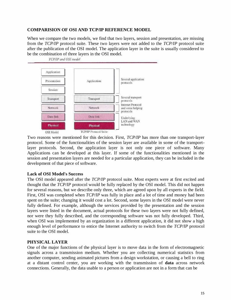
COMPARISION OF OSI AND TCP/IP REFERENCE MODEL
When we compare the two models, we find that two layers, session and presentation, are missing from the TCP/IP protocol suite. These two layers were not added to the TCP/IP protocol suite
after the publication of the OSI model. The application layer in the suite is usually considered to
be the combination of three layers in the OSI model.
Two reasons were mentioned for this decision. First, TCP/IP has more than one transport-layer
protocol. Some of the functionalities of the session layer are available in some of the transport-
layer protocols. Second, the application layer is not only one piece of software. Many
Applications can be developed at this layer. If some of the functionalities mentioned in the
session and presentation layers are needed for a particular application, they can be included in the
development of that piece of software.
Lack of OSI Model's Success The OSI model appeared after the TCP/IP protocol suite. Most experts were at first excited and
thought that the TCP/IP protocol would be fully replaced by the OSI model. This did not happen
for several reasons, but we describe only three, which are agreed upon by all experts in the field.
First, OSI was completed when TCP/IP was fully in place and a lot of time and money had been
spent on the suite; changing it would cost a lot. Second, some layers in the OSI model were never
fully defined. For example, although the services provided by the presentation and the session
layers were listed in the document, actual protocols for these two layers were not fully defined,
nor were they fully described, and the corresponding software was not fully developed. Third,
when OSI was implemented by an organization in a different application, it did not show a high
enough level of performance to entice the Internet authority to switch from the TCP/IP protocol
suite to the OSI model.
PHYSICAL LAYER One of the major functions of the physical layer is to move data in the form of electromagnetic
signals across a transmission medium. Whether you are collecting numerical statistics from
another computer, sending animated pictures from a design workstation, or causing a bell to ring at a distant control center, you are working with the transmission of data across network
connections. Generally, the data usable to a person or application are not in a form that can be

16
transmitted over a network. For example, a photograph must first be changed to a form that
transmission media can accept. Transmission media work by conducting energy along a physical path. For transmission, data needs to be changed to signals.
TRANSMISSION MEDIA Transmission media are actually located below the physical layer and are directly controlled by the physical layer. We could say that transmission media belong to layer zero. Below figure
shows the position of transmission media in relation to the physical layer.
In telecommunications, transmission media can be divided into two broad categories: guided and unguided. Guided media include twisted-pair cable, coaxial cable, and fiber-
optic cable. Unguided medium is free space.
GUIDED MEDIA Guided media, which are those that provide a conduit from one device to another, include
twisted-pair cable, coaxial cable, and fiber-optic cable. A signal traveling along any of these media is directed and contained by the physical limits of the medium. Twisted-pair and coaxial
cable use metallic (copper) conductors that accept and transport signals in the form of electric
current. Optical fiber is a cable that accepts and transports signals in the form of light. Twisted-Pair Cable A twisted pair consists of two conductors (normally copper), each with its own plastic insulation, twisted together, as shown in following figure.

17
One of the wires is used to carry signals to the receiver, and the other is used only as a ground
reference. The receiver uses the difference between the two. In addition to the signal sent by the
sender on one of the wires, interference (noise) and crosstalk may affect both wires and create
unwanted signals. If the two wires are parallel, the effect of these unwanted signals is not the
same in both wires because they are at different locations relative to the noise or crosstalk
sources (e.g., one is closer and the other is farther). This results in a difference at the receiver. By
twisting the pairs, a balance is maintained. For example, suppose in one twist, one wire is closer
to the noise source and the other is farther; in the next twist, the reverse is true. Twisting makes it
probable that both wires are equally affected by external influences (noise or crosstalk). This
means that the receiver, which calculates the difference between the two, receives no unwanted
signals. The unwanted signals are mostly canceled out. From the above discussion, it is clear that
the number of twists per unit of length (e.g., inch) has some effect on the quality of the cable.
Unshielded Versus Shielded Twisted-Pair Cable The most common twisted-pair cable used in communications is referred to as unshielded
twisted-pair (UTP). IBM has also produced a version of twisted-pair cable for its use, called
shielded twisted-pair (STP). STP cable has a metal foil or braided mesh covering that encases
each pair of insulated conductors. Although metal casing improves the quality of cable by preventing the penetration of noise or crosstalk, it is bulkier and more expensive. Below figure
Categories The Electronic Industries Association (EIA) has developed standards to classify unshielded
twisted-pair cable into seven categories. Categories are determined by cable quality, with 1 as the
lowest and 7 as the highest. Each EIA category is suitable for specific uses. Table below shows these categories.
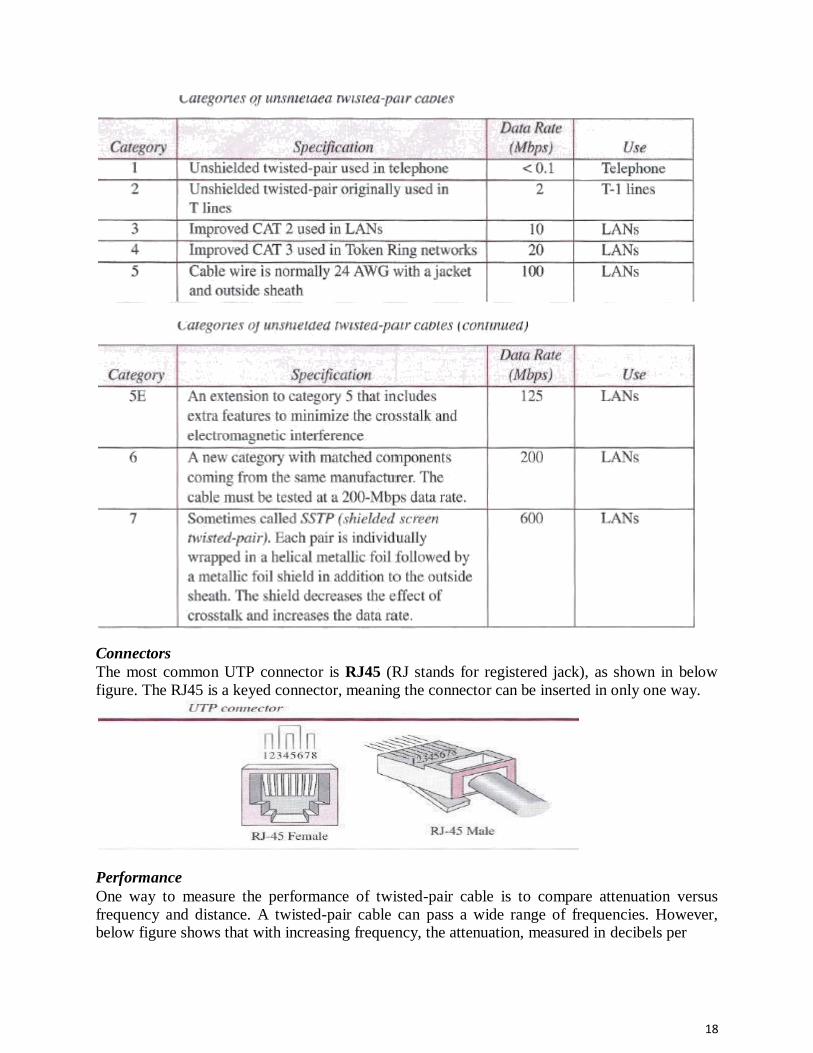
18
Connectors The most common UTP connector is RJ45 (RJ stands for registered jack), as shown in below
figure. The RJ45 is a keyed connector, meaning the connector can be inserted in only one way.
Performance One way to measure the performance of twisted-pair cable is to compare attenuation versus
frequency and distance. A twisted-pair cable can pass a wide range of frequencies. However, below figure shows that with increasing frequency, the attenuation, measured in decibels per

19
kilometer (dB/km), sharply increases with frequencies above 100 kHz. Note that gauge is a measure of the thickness of the wire.
Applications Twisted-pair cables are used in telephone lines to provide voice and data channels. The local loop-the line that connects subscribers to the central telephone office commonly consists of
unshielded twisted-pair cables. The DSL lines that are used by the telephone companies to provide high-data-rate connections also use the high-bandwidth capability of unshielded twisted-pair cables.
Local-area networks, such as lOBase-T and lOOBase-T, also use twisted-pair cables.
Coaxial Cable Coaxial cable (or coax) carries signals of higher frequency ranges than those in twisted pair
cable, in part because the two media are constructed quite differently. Instead of having two
wires, coax has a central core conductor of solid or stranded wire (usually copper) enclosed in an
insulating sheath, which is, in turn, encased in an outer conductor of metal foil, braid, or a
combination of the two. The outer metallic wrapping serves both as a shield against noise and as
the second conductor, which completes the circuit. This outer conductor is also enclosed in an
insulating sheath, and the whole cable is protected by a plastic cover.

20
Coaxial Cable Standards Coaxial cables are categorized by their Radio Government (RG) ratings. Each RG number
denotes a unique set of physical specifications, including the wire gauge of the inner conductor,
the thickness and type of the inner insulator, the construction of the shield, and the size and type of the outer casing. Each cable defined by an RG rating is adapted for a specialized function, as
shown in below table.
Coaxial Cable Connectors To connect coaxial cable to devices, we need coaxial connectors. The most common type of
connector used today is the Bayonet Neill-Concelman (BNC) connector. Below figure shows three popular types of these connectors: the BNC connector, the BNC T connector, and the BNC
terminator.
The BNC connector is used to connect the end of the cable to a device, such as a TV set. The
BNC T connector is used in Ethernet networks (see Chapter 13) to branch out to a connection to
a computer or other device. The BNC terminator is used at the end of the cable to prevent the reflection of the signal.

21
Performance As we did with twisted-pair cable, we can measure the performance of a coaxial cable. We notice
in Figure 7.9 that the attenuation is much higher in coaxial cable than in twisted-pair cable. In other words, although coaxial cable has a much higher bandwidth, the signal weakens rapidly
and requires the frequent use of repeaters.
Applications Coaxial cable was widely used in analog telephone networks where a single coaxial network
could carry 10,000 voice signals. Later it was used in digital telephone networks where a single coaxial cable could carry digital data up to 600 Mbps. However, coaxial cable in telephone
networks has largely been replaced today with fiber optic cable.
Cable TV networks also use coaxial cables. In the traditional cable TV network, the entire
network used coaxial cable. Later, however, cable TV providers replaced most of the media with
fiber-optic cable; hybrid networks use coaxial cable only at the network boundaries, near the
consumer premises. Cable TV uses RG-59 coaxial cable. Another common application of coaxial
cable is in traditional Ethernet LANs (see Because of its high bandwidth, and consequently high
data rate, coaxial cable was chosen for digital transmission in early Ethernet LANs. The lOBase-
2, or Thin Ethernet, uses RG-58 coaxial cable with BNC connectors to transmit data at 10 Mbps
with a range of 185 m. The lOBase5, or Thick Ethernet, uses RG-ll (thick coaxial cable) to
transmit 10 Mbps with a range of 5000 m. Thick Ethernet has specialized connectors.
Fiber-Optic Cable A fiber-optic cable is made of glass or plastic and transmits signals in the form of light. To understand optical fiber, we first need to explore several aspects of the nature of light. Light
travels in a straight line as long as it is moving through a single uniform substance. If a ray of

22
light traveling through one substance suddenly enters another substance (of a different density),
the ray changes direction. Below figure shows how a ray of light changes direction when going
from a denser to a less dense substance. As the figure shows, if the angle of incidence I (the
angle the ray makes with the line perpendicular to the interface between the two substances) is
less than the critical angle, the ray refracts and moves closer to the surface. If the angle of
incidence is equal to the critical angle, the light bends along the interface. If the angle is greater
than the critical angle, the ray reflects (makes a turn) and travels again in the denser
substance . Note that the critical angle is a property of the substance, and its value differs from
one substance to another. Optical fibers use reflection to guide light through a channel. A glass or
plastic core is surrounded by a cladding of less dense glass or plastic. The difference in density of the two materials must be such that a beam of light moving through the core is reflected off the
cladding instead of being refracted into it. See below figure.
Propagation Modes Current technology supports two modes (multimode and single mode) for propagating light along optical channels, each requiring fiber with different physical characteristics. Multimode
can be implemented in two forms: step-index or graded-index .

23
Multimode Multimode is so named because multiple beams from a light source move through the core in
different paths. How these beams move within the cable depends on the structure of the core.
In multimode step-index fiber, the density of the core remains constant from the center to the
edges. A beam of light moves through this constant density in a straight line until it reaches the
interface of the core and the cladding. A second type of fiber, called multimode graded-index
fiber, decreases this distortion of the signal through the cable. The word index here refers to the
index of refraction. As we saw above, the index of refraction is related to density. Single-Mode
uses step-index fiber and a highly focused source of light that limits beams to a small range of
angles, all close to the horizontal. The single-mode fiber itself is manufactured with a much
smaller diameter than that of multimode fiber, and with substantially lowers density (index of
refraction). The decrease in density results in a critical angle that is close enough to 90°

24
to make the propagation of beams almost horizontal. In this case, propagation of different beams
is almost identical, and delays are negligible. All the beams arrive at the destination "together" and can be recombined with little distortion to the signal.
Fiber Sizes Optical fibers are defined by the ratio of the diameter of their core to the diameter of their cladding, both expressed in micrometers. The common sizes are shown in below table. Note that
the last size listed is for single-mode only.
Cable Composition Following figure shows the composition of a typical fiber-optic cable. The outer jacket is made
of either pvc or Teflon. Inside the jacket are Kevlar strands to strengthen the cable. Kevlar is a
strong material used in the fabrication of bulletproof vests. Below the Kevlar is another plastic coating to cushion the fiber. The fiber is at the center of the cable, and it consists of cladding and
core.
Fiber-Optic Cable Connectors There are three types of connectors for fiber-optic cables, as shown in below figure. The
subscriber channel (SC) connector is used for cable TV. It uses a push/pull locking system. The
straight-tip (ST) connector is used for connecting cable to networking devices. It uses a bayonet
locking system and is more reliable than sc. MT-RJ is a connector that is the same size as RJ45.
Performance The plot of attenuation versus wavelength in Figure 7.16 shows a very interesting phenomenon in
fiber-optic cable. Attenuation is flatter than in the case of twisted-pair cable and coaxial cable.
The performance is such that we need fewer (actually one tenth as many) repeaters when we use fiber-optic cable.

25
Applications Fiber-optic cable is often found in backbone networks because its wide bandwidth is cost-
effective. Today, with wavelength-division multiplexing (WDM), we can transfer data at a rate of 1600 Gbps. The SONET network that we discuss in Chapter 14 provides such a backbone. Some cable TV companies use a combination of optical fiber and coaxial cable, thus creating a
hybrid network. Optical fiber provides the backbone structure while coaxial cable provides the
connection to the user premises. This is a cost-effective configuration since the narrow
bandwidth requirement at the user end does not justify the use of optical fiber. Local-area
networks such as 100Base-FX network (Fast Ethernet) and 1000Base-X also use fiber-optic
cable.

26
Advantages and Disadvantages of Optical Fiber
Advantages
Fiber-optic cable has several advantages over metallic cable (twisted-pair or coaxial).
➢ Higher bandwidth. Fiber-optic cable can support dramatically higher bandwidths (and hence data rates) than either twisted-pair or coaxial cable. Currently, data rates and bandwidth utilization over fiber-optic cable are limited not by the medium but by the signal generation and reception technology available.
➢ Less signal attenuation. Fiber-optic transmission distance is significantly greater than that of other guided media. A signal can run for 50 km without requiring regeneration. We need repeaters every 5 km for coaxial or twisted-pair cable.
➢ D Immunity to electromagnetic interference. Electromagnetic noise cannot affect fiber-optic cables.
➢ D Resistance to corrosive materials. Glass is more resistant to corrosive materials than copper.
➢ Light weight. Fiber-optic cables are much lighter than copper cables.
➢ Greater immunity to tapping. Fiber-optic cables are more immune to tapping than copper cables. Copper cables create antenna effects that can easily be tapped.
Disadvantages There are some disadvantages in the use of optical fiber.
➢ Installation and maintenance. Fiber-optic cable is a relatively new technology. Its installation and maintenance require expertise that is not yet available everywhere. o Unidirectional light propagation. Propagation of light is unidirectional. If we need bidirectional communication, two fibers are needed.
➢ Cost. The cable and the interfaces are relatively more expensive than those of other guided media. If the demand for bandwidth is not high, often the use of optical fiber cannot be justified.
UNGUIDED MEDIA: WIRELESS Unguided medium transport electromagnetic waves without using a physical conductor. This
type of communication is often referred to as wireless communication. Signals are normally
broadcast through free space and thus are available to anyone who has a device capable of
receiving them. Below figure 7.17 shows the part of the electromagnetic spectrum, ranging from
3 kHz to 900 THz, used for wireless communication. Unguided signals can travel from the
source to the destination in several ways: ground propagation, sky propagation, and line-of-sight
propagation, as shown in below figure.

27
In ground propagation, radio waves travel through the lowest portion of the atmosphere,
hugging the earth. These low-frequency signals emanate in all directions from the transmitting
antenna and follow the curvature of the planet. Distance depends on the amount of power in the
signal: The greater the power, the greater the distance. In sky propagation, higher-frequency
radio waves radiate upward into the ionosphere (the layer of atmosphere where particles exist as
ions) where they are reflected back to earth. This type of transmission allows for greater
distances with lower output power. In line-of-sight propagation, very high-frequency signals
are transmitted in straight lines directly from antenna to antenna.
The section of the electromagnetic spectrum defined as radio waves and microwaves is divided
into eight ranges, called bands, each regulated by government authorities. These bands are rated
from very low frequency (VLF) to extremely high frequency (EHF). Below table lists these
bands, their ranges, propagation methods, and some applications

28
Radio Waves Although there is no clear-cut demarcation between radio waves and microwaves,
electromagnetic waves ranging in frequencies between 3 kHz and 1 GHz are normally called
radio waves; waves ranging in frequencies between I and 300 GHz are called microwaves.
However, the behavior of the waves, rather than the frequencies, is a better criterion for
classification. Radio waves, for the most part, are Omni-directional. When an antenna transmits
radio waves, they are propagated in all directions. This means that the sending and receiving
antennas do not have to be aligned. A sending antenna sends waves that can be received by any
receiving antenna. The Omni-directional property has a disadvantage, too. The radio waves
transmitted by one antenna are susceptible to interference by another antenna that may send
signals using the same frequency or band. Radio waves, particularly those waves that propagate
in the sky mode, can travel long distances. This makes radio waves a good candidate for long-
distance broadcasting such as AM radio.
Omni directional Antenna Radio waves use Omni directional antennas that send out signals in all directions. Based on the
wavelength, strength, and the purpose of transmission, we can have several types of antennas.
Below Figure shows an Omni directional antenna.

29
Applications The Omni directional characteristics of radio waves make them useful for multicasting, in which there is one sender but many receivers. AM and FM radio, television, maritime radio, cordless
phones, and paging are examples of multicasting. Radio waves are used for multicast communications,
such as radio and television, and paging systems.
Microwaves
Electromagnetic waves having frequencies between 1 and 300 GHz are called microwaves.
Microwaves are unidirectional. When an antenna transmits microwaves, they can be narrowly
focused. This means that the sending and receiving antennas need to be aligned. The
unidirectional property has an obvious advantage. A pair of antennas can be aligned without interfering with another pair of aligned antennas.
The following describes some characteristics of microwave propagation: ➢ Microwave propagation is line-of-sight. Since the towers with the mounted antennas need
to be in direct sight of each other, towers that are far apart need to be very tall. The curvature of the earth as well as other blocking obstacles does not allow two short towers to communicate by using microwaves. Repeaters are often needed for long distance communication.
➢ Very high-frequency microwaves cannot penetrate walls. This characteristic can be a disadvantage if receivers are inside buildings.
➢ The microwave band is relatively wide, almost 299 GHz. Therefore wider sub bands can be assigned, and a high data rate is possible.
➢ Use of certain portions of the band requires permission from authorities.
Unidirectional Antenna Microwaves need unidirectional antennas that send out signals in one direction. Two types of
antennas are used for microwave communications: the parabolic dish and the horn .

30
A parabolic dish antenna is based on the geometry of a parabola: Every line parallel to the line of
symmetry (line of sight) reflects off the curve at angles such that all the lines intersect in a
common point called the focus. The parabolic dish works as a funnel, catching a wide range of
waves and directing them to a common point. In this way, more of the signal is recovered than would be possible with a single-point receiver. Outgoing transmissions are broadcast through a horn aimed at the dish. The microwaves hit the dish and are deflected outward in a reversal of the receipt path. A horn antenna looks like a gigantic scoop. Outgoing transmissions are broadcast up a stem (resembling a handle) and
deflected outward in a series of narrow parallel beams by the curved head. Received
transmissions are collected by the scooped shape of the horn, in a manner similar to the parabolic
dish, and are deflected down into the stem.
Applications Microwaves, due to their unidirectional properties, are very useful when unicast (one to- one) communication is needed between the sender and the receiver. They are used in cellular phone,
satellite networks, and wireless LANs Microwaves are used for unicast communication such as cellular telephones, satellite
networks, and wireless LANs.
Infrared Infrared waves, with frequencies from 300 GHz to 400 THz (wavelengths from 1 mm to 770
nrn), can be used for short-range communication. Infrared waves, having high frequencies,
cannot penetrate walls. This advantageous characteristic prevents interference between one
system and another; a short-range communication system in one room cannot be affected by
another system in the next room. When we use our infrared remote control, we do not interfere
with the use of the remote by our neighbors. However, this same characteristic makes infrared
signals useless for long-range communication. In addition, we cannot use infrared waves outside
a building because the sun's rays contain infrared waves that can interfere with the
communication.
Applications The infrared band, almost 400 THz, has an excellent potential for data transmission. Such a wide
bandwidth can be used to transmit digital data with a very high data rate. The Infrared Data
Association elrDA), an association for sponsoring the use of infrared waves, has established
standards for using these signals for communication between devices such as keyboards, mice,
PCs, and printers. For example, some manufacturers provide a special port called the IrDA port
that allows a wireless keyboard to communicate with a PC. The standard originally defined a
data rate of 75 kbps for a distance up to 8 m. The recent standard defines a data rate of 4 Mbps. Infrared signals defined by IrDA transmit through line of sight; the IrDA port on the keyboard
needs to point to the PC for transmission to occur. Infrared signals can be used for short-range communication in a closed area using line-of-sight propagation.
DATA-LINK LAYER The Internet is a combination of networks glued together by connecting devices (routers or
switches). If a packet is to travel from a host to another host, it needs to pass through these networks. Below figure shows the same scenario. Communication at the data-link layer is made
up of five separate logical connections between the data-link layers in the path.

31
Design Issues: The data-link layer is located between the physical and the network layers. The data link layer
provides services to the network layer; it receives services from the physical layer. Let us discuss services provided by the data-link layer. The duty scope of the data-link layer is node-to-node.
When a packet is travelling in the Internet, the data-link layer of a node (host or router) is
responsible for delivering a datagram to the next node in the path. For this purpose, the data-link layer of the sending node needs to encapsulate the datagram
received from the network in a frame, and the data-link layer of the receiving node needs to
decapsulate the datagram from the frame. In other words, the data-link layer of the source host
needs only to encapsulate, the data-link layer of the destination host needs to decapsulate, but
each intermediate node needs to both encapsulate and decapsulate. One may ask why we need
encapsulation and decapsulation at each intermediate node. The reason is that each link may be
using a different protocol with a different frame format. Even if one link and the next are using
the same protocol, encapsulation and decapsulation are needed because the link-layer addresses
are normally different. An analogy may help in this case. Assume a person needs to travel from
her home to her friend's home in another city. The traveller can use three transportation tools. She can take a taxi to go to the train station in her
own city, then travel on the train from her own city to the city where her friend lives, and finally

32
reach her friend's home using another taxi. Here we have a source node, a destination node, and
two intermediate nodes. The traveller needs to get into the taxi at the source node, get out of the
taxi and get into the train at the first intermediate node (train station in the city where she lives),
get out of the train and get into another taxi at the second intermediate node (train station in the
city where her friend lives), and finally get out of the taxi when she arrives at her destination. A
kind of encapsulation occurs at the source node, encapsulation and decapsulation occur at the
intermediate nodes, and decapsulation occurs at the destination node. For simplicity, we have
assumed that we have only one router between the source and destination. The datagram received
by the data-link layer of the source host is encapsulated in a frame. The frame is logically
transported from the source host to the router. The frame is decapsulated at the data-link layer of
the router and encapsulated at another frame. The new frame is logically transported from the
router to the destination host. Note that, although we have shown only two data-link layers at the
router, the router actually has three data-link layers because it is connected to three physical
links.
Framing Definitely, the first service provided by the data-link layer is framing. The data-link layer at each
node needs to encapsulate the datagram (packet received from the network layer) in a frame
before sending it to the next node. The node also needs to decapsulate the datagram from the
frame received on the logical channel. Although we have shown only a header for a frame, we
will see in future chapters that a frame may have both a header and a trailer. Different data-link
layers have different formats for framing. A packet at the data-link layer is normally called a
frame.
Flow Control Whenever we have a producer and a consumer, we need to think about flow control. If the
producer produces items that cannot be consumed, accumulation of items occurs. The sending data-link layer at the end of a link is a producer of frames; the receiving data-link layer at the

33
other end of a link is a consumer. If the rate of produced frames is higher than the rate of
consumed frames, frames at the receiving end need to be buffered while waiting to be consumed
(processed). Definitely, we cannot have an unlimited buffer size at the receiving side. We have
two choices. The first choice is to let the receiving data-link layer drop the frames if its buffer is
full. The second choice is to let the receiving data-link layer send a feedback to the sending data-
link layer to ask it to stop or slow down. Different data-link-layer protocols use different
strategies for flow control. Since flow control also occurs at the transport layer, with a higher
degree of importance, we discuss this issue in Chapter 23 when we talk about the transport layer.
Error Control At the sending node, a frame in a data-link layer needs to be changed to bits, transformed to
electromagnetic signals, and transmitted through the transmission media. At the receiving node,
electromagnetic signals are received, transformed to bits, and put together to create a frame.
Since electromagnetic signals are susceptible to error, a frame is susceptible to error. The error
needs first to be detected. After detection, it needs to be either corrected at the receiver node or
discarded and retransmitted by the sending node. Since error detection and correction is an issue
in every layer (node-to node or host-to-host).
Congestion Control Although a link may be congested with frames, which may result in frame loss, most data-link-
layer protocols do not directly use a congestion control to alleviate congestion, although some
wide-area networks do. In general, congestion control is considered an issue in the network layer or the transport layer because of its end-to-end nature.
CYCLIC CODES Cyclic codes are special linear block codes with one extra property. In a cyclic code, if a
codeword is cyclically shifted (rotated), the result is another codeword. For example, if 1011000
is a codeword and we cyclically left-shift, then 0110001 is also a codeword. In this case, if we
call the bits in the first word ao to a6, and the bits in the second word bo to b6, we can shift the bits by using the following: In the rightmost equation, the last bit of the first word is wrapped
around and becomes the first bit of the second word.
Cyclic Redundancy Check We can create cyclic codes to correct errors. However, the theoretical background required is
beyond the scope of this book. In this section, we simply discuss a subset of cyclic codes called the cyclic redundancy check (CRC), which is used in networks such as LANs and WANs. Table
below shows an example of a CRC code. We can see both the linear and cyclic properties of this
code.

34
Figure below shows one possible design for the encoder and decoder.
In the encoder, the data word has k bits (4 here); the codeword has n bits (7 here). The size of
the data word is augmented by adding n - k (3 here) Os to the right-hand side of the word. The
n-bit result is fed into the generator. The generator uses a divisor of size n - k + 1 (4 here),
predefined and agreed upon. The generator divides the augmented data word by the divisor
(modulo-2 division). The quotient of the division is discarded; the remainder (r2rlrO) is
appended to the data word to create the codeword. The decoder receives the codeword (possibly
corrupted in transition). A copy of all n bits is fed to the checker, which is a replica of the
generator. The remainder produced by the checker is a syndrome of n - k (3 here) bits, which is
fed to the decision logic analyzer. The analyzer has a simple function. If the syndrome bits are
all Os, the 4 leftmost bits of the codeword are accepted as the data word (interpreted as no
error); otherwise, the 4 bits are discarded (error).

35
Encoder Let us take a closer look at the encoder. The encoder takes a data word and augments it with n - k number of Os. It then divides the augmented data word by the divisor, as shown in below figure.
Decoder The codeword can change during transmission. The decoder does the same division process as
the encoder. The remainder of the division is the syndrome. If the syndrome is all Os, there is no
error with a high probability; the data word is separated from the received codeword and
accepted. Otherwise, everything is discarded. Figure 10.7 shows two cases: The left-hand figure
shows the value of the syndrome when no error has occurred; the syndrome is 000. The right-
hand part of the figure shows the case in which there is a single error. The syndrome is not all Os
(it is 011).

36
ELEMENT DATA LINK PROTOCOLS AND SLIDING WINDOW PROTOCOL
Traditionally four protocols have been defined for the data-link layer to deal with flow and error
control: Simple, Stop-and-Wait, Go-Back-N, and Selective-Repeat. Although the first two protocols still are used at the data-link layer, the last two have disappeared.
Simple Protocol Our first protocol is a simple protocol with neither flow nor error control. We assume that the
receiver can immediately handle any frame it receives. In other words, the receiver can never be overwhelmed with incoming frames. Below figure shows the layout for this protocol.
The data-link layer at the sender gets a packet from its network layer, makes a frame out of it,
and sends the frame. The data-link layer at the receiver receives a frame from the link, extracts
the packet from the frame, and delivers the packet to its network layer. The data-link layers of the sender and receiver provide transmission services for their network layers.

37
Stop-and- Wait Protocol Our second protocol is called the Stop-and- Wait protocol, which uses both flow and error
control. We show a primitive version of this protocol here, but we discuss the more sophisticated
version in Chapter 23 when we have learned about sliding windows. In this protocol, the sender
sends one frame at a time and waits for an acknowledgment before sending the next one. To
detect corrupted frames, we need to add a CRC to each data frame. When a frame arrives at the
receiver site, it is checked. If its CRC is incorrect, the frame is corrupted and silently discarded.
The silence of the receiver is a signal for the sender that a frame was either corrupted or lost.
Every time the sender sends a frame, it starts a timer. If an acknowledgment arrives before the
timer expires, the timer is stopped and the sender sends the next frame (if it has one to send). If
the timer expires, the sender resends the previous frame, assuming that the frame was either lost
or corrupted. This means that the sender needs to keep a copy of the frame until its
acknowledgment arrives. When the corresponding acknowledgment arrives, the sender discards
the copy and sends the next frame if it is ready. Below figure shows the outline for the Stop-and-
Wait protocol. Note that only one frame and one acknowledgment can be in the channels at any
time.
HDLC High-level Data Link Control (HDLC) is a bit-oriented protocol for communication over point -
to-point and multipoint links. It implements the Stop-and- Wait protocol we discussed earlier.
Although this protocol is more a theoretical issue than practical, most of the concept defined in
this protocol is the basis for other practical protocols such as PPP, which we discuss next, or the Ethernet protocol.
Configurations and Transfer Modes
HDLC provides two common transfer modes that can be used in different configurations:
Normal response mode (NRM) and Asynchronous balanced mode (ABM) In normal response mode (NRM), the station configuration is unbalanced. We have one primary
station and multiple secondary stations. A primary station can send commands; a secondary
station can only respond. The NRM is used for both point-to-point and multipoint links, as
shown in below Figure. In ABM, the configuration is balanced. The link is point-to-point, and
each station can function as a primary and a secondary (acting as peers) this is the common mode
today.

38
link itself. Each frame in HDLC may contain up to six fields: a beginning flag field, an address field, a control field, an information field, a frame check sequence (FCS) field, and an ending flag field. In multiple-frame transmissions, the ending flag of one frame can serve as the
beginning flag of the next frame.

39
Let us now discuss the fields and their use in different frame types. ➢ D Flag field. This field contains synchronization pattern 01111110, which identifies both the
beginning and the end of a frame.
➢ D Address field. This field contains the address of the secondary station. If a primary station created the frame, it contains a to address. If a secondary station creates the frame, it contains a from address. The address field can be one byte or several bytes long, depending on the needs of the network.
• Control field. The control field is one or two bytes used for flow and error control. • Information field. The information field contains the user's data from the network
layer or management information. Its length can vary from one network to another.
• FCS field. The frame check sequence (FCS) is the HDLC error detection field. It can contain either a 2- or 4-byte CRC.
The control field determines the type of frame and defines its functionality. So let us discuss the format of this field in detail. The format is specific for the type of frame, as shown in below
Figure.
Control Field for I-Frames
I- frames are designed to carry user data from the network layer. In addition, they can include
flow- and error-control information (piggybacking). The subfields in the control field are used to
define these functions. The first bit defines the type. If the first bit of the control field is 0, this
means the frame is an I-frame. The next 3 bits, called N(S), define the sequence number of the
frame. Note that with 3 bits, we can define a sequence number between 0 and 7. The last 3 bits,
called N(R), correspond to the acknowledgment number when piggybacking is used. The single
bit between N(S) and N(R) is called the PIF bit. The PIF field is a single bit with a dual purpose.
It has meaning only when it is set (bit = 1) and can mean poll or final. It means poll when the
frame is sent by a primary station to a secondary (when the address field contains the address of
the receiver). It means final when the frame is sent by a secondary to a primary (when the
address field contains the address of the sender).
Control Field for S-Frames Supervisory frames are used for flow and error control whenever piggybacking is either
impossible or inappropriate. S-frames do not have information fields. If the first 2 bits of the
control field are 10, this means the frame is an S-frame. The last 3 bits, called N(R), correspond
to the acknowledgment number (ACK) or negative acknowledgment number (NAK), depending
on the type of S-frame. The 2 bits called code are used to define the type of S-frame itself. With
2 bits, we can have four types of S-frames, as described below:

40
• Receive ready (RR) If the value of the code subfield is 00, it is an RR S-frame.
This kind of frame acknowledges the receipt of a safe and sound frame or group
of frames. In this case, the value of the N(R) field defines the acknowledgment
number.
• Receive not ready (RNR) If the value of the code subfield is 10, it is an RNR S
frame. This kind of frame is an RR frame with additional functions. It
acknowledges the receipt of a frame or group of frames, and it announces that the
receiver is busy and cannot receive more frames. It acts as a kind of congestion-
control mechanism by asking the sender to slow down. The value of N(R) is the
acknowledgment number.
• Reject (REJ) If the value of the code subfield is 01, it is an REJ S-frame. This is a
NAK frame, but not like the one used for Selective Repeat ARQ. It is a NAK that
can be used in Go-Back-N ARQ to improve the efficiency of the process by
informing the sender, before the sender timer expires, that the last frame is lost or
damaged. The value of N(R) is the negative acknowledgment number.
• Selective reject (SREJ) If the value of the code subfield is 11, it is an SREJ S
frame. This is a NAK frame used in Selective Repeat ARQ. Note that the HDLC
Protocol uses the term selective reject instead of selective repeat. The value of
N(R) is the negative acknowledgment number.
Control Field or V-Frames Unnumbered frames are used to exchange session management and control information between
connected devices. Unlike S-frames, U-frames contain an information field, but one used for
system management information, not user data. As with S-frames, however, much of the information carried by If-frames is contained in codes included in the control field. If-frame codes are divided into two sections: a 2-bit prefix before the PI F bit and a 3-bit suffix after the PIP bit. Together, these two segments (5 bits) can be used to create up
to 32 different types of U-frames.
Control Field for V-Frames Unnumbered frames are used to exchange session management and control information between
connected devices. Unlike S-frames, U-frames contain an information field, but one used for
system management information, not user data. As with S-frames, however, much of the
information carried by U-frames is contained in codes included in the control field. U-frame
codes are divided into two sections: a 2-bit prefix before the PIP bit and a 3-bit suffix after the
P/F bit. Together, these two segments (5 bits) can be used to create up to 32 different types of If-
frames.
POINT-TO-POINT PROTOCOL (PPP) One of the most common protocols for point-to-point access is the Point-to-Point Protocol
(PPP). Today, millions of Internet users who need to connect their home computers to the server
of an Internet service provider use PPP. The majority of these users have a traditional modem;
they are connected to the Internet through a telephone line, which provides the services of the
physical layer. But to control and manage the transfer of data, there is a need for a point-to-point
protocol at the data-link layer. PPP is by far the most common.

41
Services The designers of PPP have included several services to make it suitable for a point-to point protocol, but have ignored some traditional services to make it simple.
Services Provided by PPP PPP defines the format of the frame to be exchanged between devices. It also defines how two
devices can negotiate the establishment of the link and the exchange of data. PPP is designed to
accept payloads from several network layers (not only IP). Authentication is also provided in the
protocol, but it is optional. The new version of PPP, called Multilink PPP, provides connections
over multiple links. One interesting feature of PPP is that it provides network address
configuration. This is particularly useful when a home user needs a temporary network address to
connect to the Internet.
Framing PPP uses a character-oriented (or byte-oriented) frame. Below figure shows the format of a PPP frame. The description of each field follows:
• Flag A PPP frame starts and ends with a l-byte flag with the bit pattern 01111110.
o Address The address field in this protocol is a constant value and set to 11111111 (broadcast address).
• D Control This field is set to the constant value 00000011 (imitating unnumbered frames
in HDLC). As we will discuss later, PPP does not provide any flow control. Error control is also limited to error detection.
• Protocol The protocol field defines what is being carried in the data field: either user data
or other information. This field is by default 2 bytes long, but the two parties can agree to use only 1 byte.
• Payload field This field carries either the user data or other information that we will
discuss shortly. The data field is a sequence of bytes with the default of a maximum of
1500 bytes; but this can be changed during negotiation. The data field is byte-stuffed if
the flag byte pattern appears in this field. Because there is no field defining the size of the
data field, padding is needed if the size is less than the maximum default value or the
maximum negotiated value D FCS. The frame check sequence (FCS) is simply a 2-byte
or 4-byte standard CRC.

42
Byte Stuffing Since PPP is a byte-oriented protocol, the flag in PPP is a byte that needs to be escaped
whenever it appears in the data section of the frame. The escape byte is 01111101, which means that every time the flag like pattern appears in the data, this extra byte is stuffed to tell the
receiver that the next byte is not a flag. Obviously, the escape byte itself should be stuffed with
another escape byte.

43
UNIT- II
Multiple Access Protocols
Multiple Access Protocols
When nodes or stations are connected and use a common link, called a multipoint or broadcast link, we need a multiple-access protocol to coordinate access to the link. Many protocols have been devised to handle access to a shared link. All of these protocols
belong to a sub layer in the data-link layer called media access control (MAC). We categorize
them into three groups:
➢ 1 The first section discusses random-access protocols. Four protocols, ALOHA, CSMA, CSMA/CD, and CSMA/CA, are described in this section. These protocols are mostly used in LANs and WANs.
➢ 2 The second section discusses controlled-access protocols. Three protocols, reservation, polling, and token-passing, are described in this section. Some of these protocols are used in LANs, but others have some historical value.
➢ 3 The third section discusses channelization protocols. Three protocols, FDMA, TDMA, and CDMA are described in this section. These protocols are used in cellular telephony.
RANDOM ACCESS In random-access or contention methods, no station is superior to another station and none is
assigned control over another. At each instance, a station that has data to send uses a procedure
defined by the protocol to make a decision on whether or not to send. This decision depends on
the state of the medium (idle or busy). In other words, each station can transmit when it desires
on the condition that it follows the predefined procedure, including testing the state of the
medium.
Two features give this method its name:
First, there is no scheduled time for a station to transmit. Transmission is random among the
stations. That is why these methods are called random access.
Second, no rules specify which station should send next. Stations compete with one another to
access the medium. That is why these methods are also called contention methods.

44
In a random-access method, each station has the right to the medium without being controlled by
any other station. However, if more than one station tries to send, there is an access conflict-collision-and the frames will be either destroyed or modified.
ALOHA ALOHA, the earliest random access method was developed at the University of Hawaii in early 1970. It was designed for a radio (wireless) LAN, but it can be used on any shared medium. It is obvious that there are potential collisions in this arrangement. The medium is shared
between the stations. When a station sends data, another station may attempt to do so at the same time. The data from the two stations collide and become garbled.
Pure ALOHA The original ALOHA protocol is called pure ALOHA. This is a simple but elegant protocol. The
idea is that each station sends a frame whenever it has a frame to send (multiple access).
However, since there is only one channel to share, there is the possibility of collision between frames from different stations. Below figure shows an example of frame collisions in pure
ALOHA.
There are four stations (unrealistic assumption) that contend with one another for access to the
shared channel. The figure shows that each station sends two frames; there are a total of eight
frames on the shared medium. Some of these frames collide because multiple frames are in
contention for the shared channel. Above Figure shows that only two frames survive: one frame
from station 1 and one frame from station 3. We need to mention that even if one bit of a frame
coexists on the channel with one bit from another frame, there is a collision and both will be
destroyed. It is obvious that we need to resend the frames that have been destroyed during
transmission. The pure ALOHA protocol relies on acknowledgments from the receiver. When a
station sends a frame, it expects the receiver to send an acknowledgment. If the
acknowledgment does not arrive after a time-out period, the station assumes that the frame (or
the acknowledgment) has been destroyed and resends the frame. A collision involves two or
more stations. If all these stations try to resend their frames after the time-out, the frames will
collide again. Pure ALOHA dictates that when the time-out period passes, each station waits a
random amount of time before resending its frame. The randomness will help avoid more
collisions. We call this time the back off time Ts.
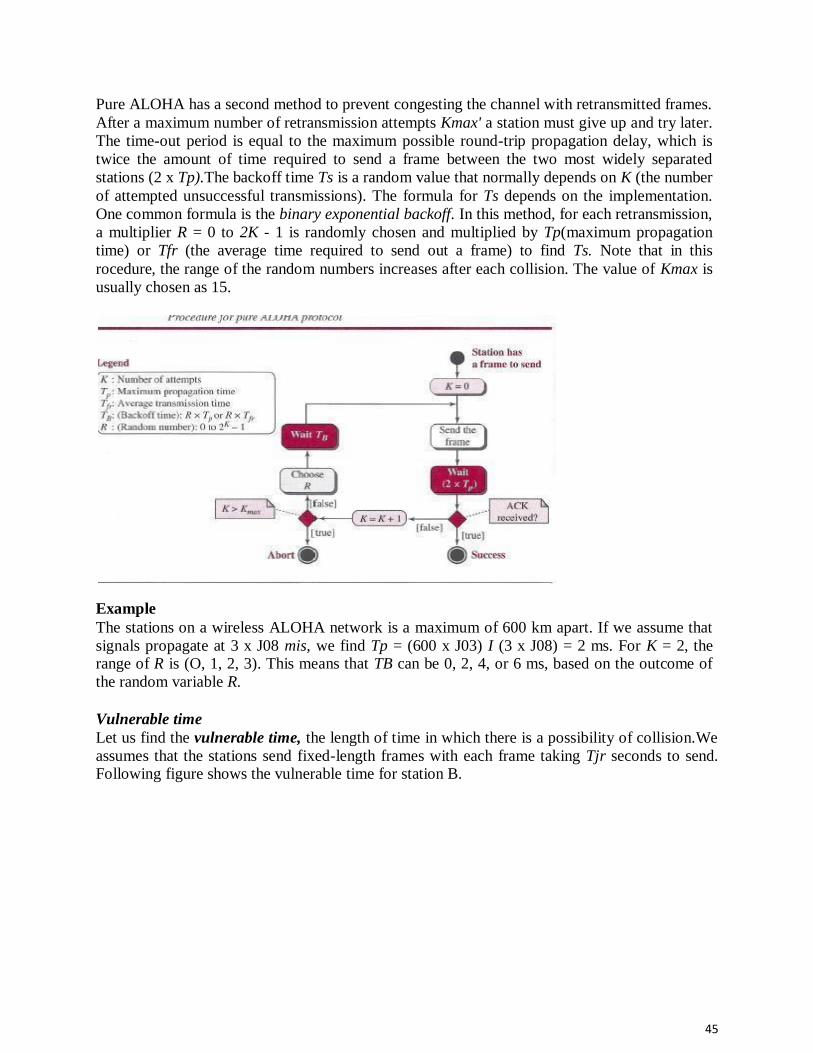
45
Pure ALOHA has a second method to prevent congesting the channel with retransmitted frames.
After a maximum number of retransmission attempts Kmax' a station must give up and try later.
The time-out period is equal to the maximum possible round-trip propagation delay, which is
twice the amount of time required to send a frame between the two most widely separated
stations (2 x Tp).The backoff time Ts is a random value that normally depends on K (the number
of attempted unsuccessful transmissions). The formula for Ts depends on the implementation.
One common formula is the binary exponential backoff. In this method, for each retransmission,
a multiplier R = 0 to 2K - 1 is randomly chosen and multiplied by Tp(maximum propagation
time) or Tfr (the average time required to send out a frame) to find Ts. Note that in this
rocedure, the range of the random numbers increases after each collision. The value of Kmax is
usually chosen as 15.
Example The stations on a wireless ALOHA network is a maximum of 600 km apart. If we assume that
signals propagate at 3 x J08 mis, we find Tp = (600 x J03) I (3 x J08) = 2 ms. For K = 2, the range of R is (O, 1, 2, 3). This means that TB can be 0, 2, 4, or 6 ms, based on the outcome of
the random variable R.
Vulnerable time Let us find the vulnerable time, the length of time in which there is a possibility of collision.We
assumes that the stations send fixed-length frames with each frame taking Tjr seconds to send. Following figure shows the vulnerable time for station B.

46
Station B starts to send a frame at time t. Now imagine station A has started to send its frame
after t - TjT' This leads to a collision between the frames from station Band station A. On the
other hand, suppose that station C starts to send a frame before time t + Tjr- Here, there is also a
collision between frames from station B and station C. Looking at Figure 12.4, we see that the
vulnerable time during which a collision may occur in pure ALOHA is 2 times the frame
transmission time. Pure ALOHA vulnerable time = 2 x Tfr
Slotted ALOHA Pure ALOHA has a vulnerable time of 2 x Tp This is so because there is no rule that defines when the station can send. A station may send soon after another station has started or just before another station has finished. Slotted ALOHA was invented to improve the efficiency of pure
ALOHA. In slotted ALOHA we divide the time into slots of Tfr seconds and force the station to send only at the beginning of the time slot. Below figure shows an example of frame collisions in slotted ALOHA.
Because a station is allowed to send only at the beginning of the synchronized time slot, if a
station misses this moment, it must wait until the beginning of the next time slot. This means that
the station which started at the beginning of this slot has already finished sending its frame. Of
course, there is still the possibility of collision if two stations try to send at the beginning of the
same time slot. However, the vulnerable time is now reduced to one-half, equal to Tjr. Below
figure shows the situation.

47
Slotted ALOHA vulnerable time = Tlr
Throughput It can be proven that the average number of successful transmissions for slotted ALOHA is S =
G x e-G
.The maximum throughput Smax is 0.368, when G = 1. In other words, if one frame is
generated during one frame transmission time, then 36.8 percent of these frames reach their destination successfully. We expect G = 1 to produce maximum throughput because the vulnerable time is equal to the frame transmission time. Therefore, if a station generates only one frame in this vulnerable time (and no other station generates a frame during this time), the frame will reach its destination successfully.
The throughput for slotted ALOHA is S = G x e-G
The maximum throughput Smax = 0.368 when G = 1.
Example A slotted ALOHA network transmits 200-bit frames using a shared channel with a 200-kbps bandwidth. Find the throughput if the system (all stations together) produces a. 1000 frames per second.
b. 500 frames per second. c. 250 frames per second.
Solution This situation is similar to the previous exercise except that the network is using slotted ALOHA instead of pure ALOHA. The frame transmission time is 200/200 kbps or 1 ms. a. In this case G is 1. So S = G x e-G = 0.368 (36.8 percent). This means that the throughput is 1000 x 0.0368 = 368 frames. Only 368 out of 1000 frames will probably
survive. Note that this is the maximum throughput case, percentagewise. b. Here G is 112. In this case S = G x e-G = 0.303 (30.3 percent). This means that the
throughput is 500 x 0.0303 = 151. Only 151 frames out of 500 will probably survive. c.
Now G is 114. In this case S = G x e-G = 0.195 (19.5 percent). This means that the
throughput is 250 x 0.195 = 49. Only 49 frames out of 250 will probably survive.
CSMA To minimize the chance of collision and, therefore, increase the performance, the CSMA method was developed. The chance of collision can be reduced if a station senses the medium before
trying to use it. Carrier sense multiple access (CSMA) requires that each station first listen to the
medium (or check the state of the medium) before sending. In other words, CSMA is based on
the principle "sense before transmit" or "listen before talk." CSMA can reduce the possibility of

48
collision, but it cannot eliminate it. The reason for this is shown in below figure, a space and
time model of a CSMA network. Stations are connected to a shared channel (usually a dedicated
medium). The possibility of collision still exists because of propagation delay; when a station
sends a frame, it still takes time (although very short) for the first bit to reach every station and
for every station to sense it. In other words, a station may sense the medium and find it idle, only
because the first bit sent by another station has not yet been received.
At time fl, station B senses the medium and finds it idle, so it sends a frame. At time t2 (t2 > tl),
station C senses the medium and finds it idle because, at this time, the first bits from station B
have not reached station C. Station C also sends a frame. The two signals collide and both frames are destroyed.
Vulnerable Time The vulnerable time for CSMA is the propagation time Tp. This is the time needed for a signal to
propagate from one end of the medium to the other. When a station sends a frame and any other
station tries to send a frame during this time, a collision will result. But if the first bi t of the
frame reaches the end of the medium, every station will already have heard the bit and will
refrain from sending. Below Figure shows the worst case. The leftmost station, A, sends a frame
at time fl, which reaches the rightmost station, D, at time tl + Tp. The gray area shows the
vulnerable area in time and space.

49
Persistence Methods What should a station do if the channel is busy? What should a station do if the channel is idle?
Three methods have been devised to answer these questions: the I-persistent method, the non
persistent method, and the p-persistent method. Below Figure shows the behavior of three persistence methods when a station finds a channel busy.
Above Figure shows the flow diagrams for these methods.
I-Persistent The l-persistent method is simple and straightforward. In this method, after the station finds the
line idle, it sends its frame immediately (with probability 1). This method has the highest chance
of collision because two or more stations may find the line idle and send their frames
immediately. We will see later that Ethernet uses this method.
Non persistent In the nonpersistent method, a station that has a frame to send senses the line. If the line is idle, it
sends immediately. If the line is not idle, it waits a random amount of time and then senses the
line again. The nonpersistent approach reduces the chance of collision because it is unlikely that
two or more stations will wait the same amount of time and retry to send simultaneously.
However, this method reduces the efficiency of the network because the medium remains idle
when there may be stations with frames to send.
P- Persistent The p-persistent method is used if the channel has time slots with a slot duration equal to or
greater than the maximum propagation time. The p-persistent approach combines the advantages
of the other two strategies. It reduces the chance of collision and improves efficiency. In this method, after the station finds the line idle it follows these Steps:

50
1. With probability p, the station sends its frame. 2. With probability q = 1- p, the station waits for the beginning of the next time slot
and checks the line again. a. If the line is idle, it goes to step 1. b. If the line is busy, it acts as though a collision has occurred and uses the back
off procedure.
CSMA/CD The CSMA method does not specify the procedure following a collision. Carrier sense multiple
access with collision detection (CSMA/CD) augments the algorithm to handle the collision. In this method, a station monitors the medium after it sends a frame to see if the transmission was
successful. If so, the station is finished. If, however, there is a collision, the frame is sent again. To better understand CSMA/CD, let us look at the first bits transmitted by the two stations
involved in the collision. Although each station continues to send bits in the frame until it detects
the collision, we show what happens as the first bits collide. In below figure, stations A and Care involved in the collision.

51
At time t1, station A has executed its persistence procedure and starts sending the bits of its
frame. At time t2, station C has not yet sensed the first bit sent by A. Station C executes its
persistence procedure and starts sending the bits in its frame, which propagate both to the left
and to the right. The collision occurs sometime after time t2' Station C detects a collision at
time t3 when it receives the first bit of A's frame. Station C immediately (or after a short time,
but we assume immediately) aborts transmission. Station A detects collision at time t4 when it
receives the first bit of C's frame; it also immediately aborts transmission. Looking at the figure,
we see that A transmits for the duration t4 - t1; C transmits for the duration t3 - t2' Now that we
know the time durations for the two transmissions, we can show a more complete graph in
below figure.
Minimum Frame Size For CSMAJCD to work, we need a restriction on the frame size. Before sending the last bit of the
frame, the sending station must detect a collision, if any, and abort the transmission. This is so
because the station, once the entire frame is sent, does not keep a copy of the frame and does not
monitor the line for collision detection. Therefore, the frame transmission time Tfr must be at
least two times the maximum propagation time Tp. To understand the reason, let us think about
the worst-case scenario. If the two stations involved in a collision are the maximum distance
apart, the signal from the first takes time Tp to reach the second, and the effect of the collision
takes another time Tp to reach the first. So the requirement is that the first station must still be
transmitting after 2Tp.
Example A network using CSMA/CD has a bandwidth of 10 Mbps. If the maximum propagation time
(including the delays in the devices and ignoring the time needed to send a jamming signal, as we see later) is 25.6I1s, what is the minimum size of the frame?

52
Solution The minimum frame transmission time is Tfr = 2 x Tp = 51.2 I1s.This means, in the worst case, a
station needs to transmit for a period of 51.2 I1sto detect the collision. The minimum size of the frame is 10Mbps x 51.211s= 512 bits or 64 bytes. This is actually the minimum size of the frame
for Standard Ethernet.
Procedure Now let us look at the flow diagram for CSMA/CD in Figure. It is similar to the one for the ALOHA protocol, but there are differences.
The first difference is the addition of the persistence process. We need to sense the channel
before we start sending the frame by using one of the persistence processes we discussed
previously (non persistent, l-persistent, or p-persistent). The second difference is the frame
transmission. In ALOHA, we first transmit the entire frame and then wait for an
acknowledgment. In CSMA/CD, transmission and collision detection are continuous processes.
We do not send the entire frame and then look for a collision. The station transmits and receives
continuously and simultaneously (using two different ports or a bidirectional port). We use a loop
to show that transmission is a continuous process. We constantly monitor in order to detect one
of two conditions: either transmission is finished or a collision is detected. Either event stops
transmission. When we come out of the loop, if a collision has not been detected, it means that
transmission is complete; the entire frame is transmitted. Otherwise, a collision has occurred. The
third difference is the sending of a short jamming signal to make sure that all other stations
become aware of the collision.
Energy Level We can say that the level of energy in a channel can have three values: zero, normal, and abnormal. At the zero level, the channel is idle. At the normal level, a station has successfully
captured the channel and is sending its frame. At the abnormal level, there is a collision and the
level of the energy is twice the normal level. A station that has a frame to send or is sending a

53
frame needs to monitor the energy level to determine if the channel is idle, busy, or in collision mode. Below figure shows the situation.
Throughput The throughput of CSMA/CD is greater than that of pure or slotted ALOHA. The maximum throughput occurs at a different value of G and is based on the persistence method and the value
of p in the p-persistent approach. For the l-persistent method, the maximum throughput is around
50 percent when G = 1. For the non persistent method, the maximum throughput can go up to 90
percent when G is between 3 and 8.
Traditional Ethernet One of the LAN protocols that used CSMA/CD is the traditional Ethernet with the data rate of 10 Mbps. The traditional Ethernet was a broadcast LAN that used the l-persistence method to
control access to the common media. Later versions of Ethernet try to move from CSMA/CD
access methods.
CSMA/CA Carrier sense multiple access with collision avoidance (CSMA/CA) was invented for wireless
networks. Collisions are avoided through the use of CSMA/CA's three strategies: the inter frame space, the contention window, and acknowledgments, as shown in below figure.

54
Inter frame Space (IFS) First, collisions are avoided by deferring transmission even if the
channel is found idle. When an idle channel is found, the station does not send immediately. It
waits for a period of time called the inter frame space or IFS. Even though the channel may
appear idle when it is sensed, a distant station may have already started transmitting. The distant
station's signal has not yet reached this station. The IFS time allows the front of the transmitted
signal by the distant station to reach this station. After waiting an IFS time, if the channel is still
idle, the station can send, but it still needs to wait a time equal to the contention window
(described next).The IFS variable can also be used to prioritize stations or frame types. For
example, a station that is assigned shorter IFS has a higher priority.
Contention Window The contention window is an amount of time divided into slots. A station
that is ready to send chooses a random number of slots as its wait time. The number of slots in
the window changes according to the binary exponential back off strategy. This means that it is
set to one slot the first time and then doubles each time the station cannot detect an idle channel
after the IFS time. This is very similar to the p-persistent method except that a random outcome
defines the number of slots taken by the waiting station. One interesting point about the
contention window is that the station needs to sense the channel after each time slot. However, if
the station finds the channel busy, it does not restart the process; it just stops the timer and
restarts it when the channel is sensed as idle. This gives priority to the station with the longest
waiting time. See below figure.
Acknowledgment With all these precautions, there still may be a collision resulting in destroyed data. In addition,
the data may be corrupted during the transmission. The positive acknowledgment and the time-out timer can help guarantee that the receiver has received the frame.
Frame Exchange Time Line
Below figure shows the exchange of data and control frames in time. 1. Before sending a frame, the source station senses the medium by checking the energy level at
the carrier frequency. a. The channel uses a persistence strategy with back off until the channel isidle. b. After the station is found to be idle, the station waits for a period of time called the DCF inter frame space (DIFS); then the station sends a control frame called the request to send
(RTS). 2. After receiving the RTS and waiting a period of time called the short inter frame space
(SIFS), the destination station sends a control frame, called the clear to send (CTS), to the
source station. This control frame indicates that the destination station is ready to receive
data.

55
3. The source station sends data after waiting an amount of time equal to SIFS. 4. The destination station, after waiting an amount of time equal to SIFS, sends an
acknowledgment to show that the frame has been received. Acknowledgment is needed in
this protocol because the station does not have any means to check for the successful arrival
of its data at the destination. On the other hand, the lack of collision in CSMA/CD is a kind
of indication to the source that data have arrived.
Network Allocation Vector How do other stations defer sending their data if one station acquires access? In other words,
how is the collision avoidance aspect of this protocol accomplished? The key is a feature called
NA V. When a station sends an RTS frame, it includes the duration of time that it needs to
occupy the channel. The stations that are affected by this transmission create a timer called a
network allocation vector (NAV) that shows how much time must pass before these stations are
allowed to check the channel for idleness. Each time a station accesses the system and sends an
RTS frame, other stations start their NAY. In other words, each station, before sensing the
physical medium to see if it is idle, first checks its NAY to see if it has expired.
Collision During Handshaking What happens if there is a collision during the time when RTS or CTS control frames are in
transition, often called the handshaking period? Two or more stations may try to send RTS
frames at the same time. These control frames may collide. However, because there is no
mechanism for collision detection, the sender assumes there has been a collision if it has not
received a CTS frame from the receiver. The back off strategy is employed, and the sender tries
again.
Hidden-Station Problem The solution to the hidden station problem is the use of the handshake frames (RTS and
CTS).Above figure also shows that the RTS message from B reaches A, but not C. However, because both Band C are within the range of A, the CTS message, which contains the duration of

56
data transmission from B to A, reaches C. Station C knows that some hidden station is using the channel and refrains from transmitting until that duration is over.
CSMAICA and Wireless Networks CSMA/CA was mostly intended for use in wireless networks. The procedure described above, however, is not sophisticated enough to handle some particular issues related to wireless
networks, such as hidden terminals or exposed terminals.
CONTROLLED ACCESS In controlled access, the stations consult one another to find which station has the right to send.
A station cannot send unless it has been authorized by other stations. We discuss three controlled-access methods.
Reservation In the reservation method, a station needs to make a reservation before sending data. Time is
divided into intervals. In each interval, a reservation frame precedes the data frames sent in that
interval. If there are N stations in the system, there are exactly N reservation mini slots in the
reservation frame. Each mini slot belongs to a station. When a station needs to send a data
frame, it makes a reservation in its own mini slot. The stations that have made reservations can
send their data frames after the reservation frame. Below figure shows a situation with five
stations and a five-mini slot reservation frame. In the first interval, only stations 1, 3, and 4 have
made reservations. In the second interval, only station 1 has made a reservation.
Polling Polling works with topologies in which one device is designated as a primary station and the
other devices are secondary stations. All data exchanges must be made through the primary
device even when the ultimate destination is a secondary device. The primary device controls the
link; the secondary devices follow its instructions. It is up to the primary device to determine
which device is allowed to use the channel at a given time. The primary device, therefore, is
always the initiator of a session This method uses poll and select functions to prevent collisions.
However, the drawback is if the primary station fails, the system goes down.
57
Select The select function is used whenever the primary device has something to send. Remember that
the primary controls the link. If the primary is neither sending nor receiving data, it knows the
link is available. If it has something to send, the primary device sends it. What it does not know,
however, is whether the target device is prepared to receive. So the primary must alert the
secondary to the upcoming transmission and wait for an acknowledgment of the secondary's
ready status. Before sending data, the primary creates and transmits a select (SEL) frame, one
field of which includes the address of the intended secondary.
Poll The poll function is used by the primary device to solicit transmissions from the secondary
devices. When the primary is ready to receive data, it must ask (poll) each device in turn if it has
anything to send. When the first secondary is approached, it responds either with a NAK frame if
it has nothing to send or with data (in the form of a data frame) if it does. If the response is
negative (a NAK frame), then the primary polls the next secondary in the same manner until it
finds one with data to send. When the response is positive (a data frame), the primary reads the
frame and returns an acknowledgment (ACK frame), verifying its receipt.
Token Passing In the token-passing method, the stations in a network are organized in a logical ring. In other
words, for each station, there is a predecessor and a successor. The predecessor is the station
which is logically before the station in the ring; the successor is the station which is after the
station in the ring. The current station is the one that is accessing the channel now. The right to
this access has been passed from the predecessor to the current station. The right will be passed
to the successor when the current station has no more data to send. But how is the right to access the channel passed from one station to another? In this method, a
special packet called a token circulates through the ring. The possession of the token gives the
station the right to access the channel and send its data. When a station has some data to send, it
waits until it receives the token from its predecessor. It then holds the token and sends its data.
When the station has no more data to send, it releases the token, passing it to the next logical
station in the ring. The station cannot send data until it receives the token again in the next round.
In this process, when a station receives the token and has no data to send, it just passes the data to
the next station. Token management is needed for this access method. Stations must be limited in the time they
can have possession of the token. The token must be monitored to ensure it has not been lost or
destroyed. For example, if a station that is holding the token fails, the token will disappear from
the network. Another function of token management is to assign priorities to the stations and to
the types of data being transmitted. And finally, token management is needed to make low-
priority stations release the token to high-priority stations.
Logical Ring In a token-passing network, stations do not have to be physically connected in a ring; the ring
can be a logical one. Below figure shows four different physical topologies that can create a logical ring.
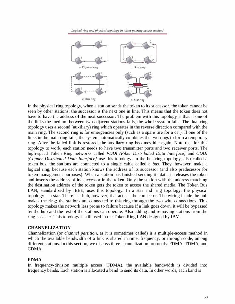
58
In the physical ring topology, when a station sends the token to its successor, the token cannot be
seen by other stations; the successor is the next one in line. This means that the token does not
have to have the address of the next successor. The problem with this topology is that if one of
the links-the medium between two adjacent stations-fails, the whole system fails. The dual ring
topology uses a second (auxiliary) ring which operates in the reverse direction compared with the
main ring. The second ring is for emergencies only (such as a spare tire for a car). If one of the
links in the main ring fails, the system automatically combines the two rings to form a temporary
ring. After the failed link is restored, the auxiliary ring becomes idle again. Note that for this
topology to work, each station needs to have two transmitter ports and two receiver ports. The
high-speed Token Ring networks called FDDI (Fiber Distributed Data Interface] and CDDI
(Copper Distributed Data Interface] use this topology. In the bus ring topology, also called a
token bus, the stations are connected to a single cable called a bus. They, however, make a
logical ring, because each station knows the address of its successor (and also predecessor for
token management purposes). When a station has finished sending its data, it releases the token
and inserts the address of its successor in the token. Only the station with the address matching
the destination address of the token gets the token to access the shared media. The Token Bus
LAN, standardized by IEEE, uses this topology. In a star and ring topology, the physical
topology is a star. There is a hub, however, that acts as the connector. The wiring inside the hub
makes the ring; the stations are connected to this ring through the two wire connections. This
topology makes the network less prone to failure because if a link goes down, it will be bypassed
by the hub and the rest of the stations can operate. Also adding and removing stations from the
ring is easier. This topology is still used in the Token Ring LAN designed by IBM.
CHANNELIZATION Channelization (or channel partition, as it is sometimes called) is a multiple-access method in
which the available bandwidth of a link is shared in time, frequency, or through code, among
different stations. In this section, we discuss three channelization protocols: FDMA, TDMA, and
CDMA.
FDMA In frequency-division multiple access (FDMA), the available bandwidth is divided into frequency bands. Each station is allocated a band to send its data. In other words, each band is
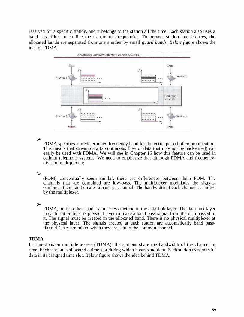
59
reserved for a specific station, and it belongs to the station all the time. Each station also uses a
band pass filter to confine the transmitter frequencies. To prevent station interferences, the
allocated bands are separated from one another by small guard bands. Below figure shows the
idea of FDMA.
➢ FDMA specifies a predetermined frequency band for the entire period of communication. This means that stream data (a continuous flow of data that may not be packetized) can easily be used with FDMA. We will see in Chapter 16 how this feature can be used in cellular telephone systems. We need to emphasize that although FDMA and frequency-division multiplexing
➢ (FDM) conceptually seem similar, there are differences between them FDM. The channels that are combined are low-pass. The multiplexer modulates the signals, combines them, and creates a band pass signal. The bandwidth of each channel is shifted by the multiplexer.
➢ FDMA, on the other hand, is an access method in the data-link layer. The data link layer in each station tells its physical layer to make a band pass signal from the data passed to it. The signal must be created in the allocated band. There is no physical multiplexer at the physical layer. The signals created at each station are automatically band pass-filtered. They are mixed when they are sent to the common channel.
TDMA In time-division multiple access (TDMA), the stations share the bandwidth of the channel in time. Each station is allocated a time slot during which it can send data. Each station transmits its
data in its assigned time slot. Below figure shows the idea behind TDMA.

60
The main problem with TDMA lies in achieving synchronization between the different stations.
Each station needs to know the beginning of its slot and the location of its slot. This may be
difficult because of propagation delays introduced in the system if the stations are spread over a
large area. To compensate for the delays, we can insert guard times. Synchronization is normally
accomplished by having some synchronization bits (normally referred to as preamble bits) at the
beginning of each slot. We also need to emphasize that although TDMA and time-division
multiplexing (TDM) conceptually seem the same, there are differences between them. TDM, as,
is a physical layer technique that combines the data from slower channels and transmits them by
using a faster channel. The process uses a physical multiplexer that interleaves data units from
each channel. TDMA, on the other hand, is an access method in the data-link layer. The data-link
layer in each station tells its physical layer to use the allocated time slot. There is no physical
multiplexer at the physical layer.
CDMA Code-division multiple access (CDMA) was conceived several decades ago. Recent advances in
electronic technology have finally made its implementation possible. CDMA differs from FDMA
in that only one channel occupies the entire bandwidth of the link. It differs from TDMA in that
all stations can send data simultaneously; there is no timesharing. In CDMA, one channel carries all transmissions simultaneously
Analogy Let us first give an analogy. CDMA simply means communication with different codes. For
example, in a large room with many people, two people can talk privately in English if nobody
else understands English. Another two people can talk in Chinese if they are the only ones who
understand Chinese, and so on. In other words, the common channel, the space of the room in
this case, can easily allow communication between several couples, but in different languages
(codes).

61
Idea Let us assume we have four stations, 1, 2,3, and 4, connected to the' same channel. The data from station 1 are d1, from station 2 are d2, and so on. The code assigned to the first station is Cj, to
the second is c2, and so on. We assume that the assigned codes have two properties.
1. If we multiply each code by another, we get O.
2. If we multiply each code by itself, we get 4 (the number of stations).
With these two properties in mind, let us see how the above four stations can send data using the same common channel, as shown in Figure.
Station 1 multiplies (a special kind of multiplication, as we will see) its data by its code to get d,.
Cj. Station 2 multiplies its data by its code to get d2 . <z- and so on. The data that go on the channel are the sum of all these terms, as shown in the box. Any station that wants to receive data from one of the other three multiplies the data on the channel by the code of the sender. For
example, suppose stations 1 and 2 are talking to each other. Station 2 wants to hear what station 1 is saying. It multiplies the data on the channel by C r- the code of station 1.
Because (cI . cI) is 4, but (c2 . cl), (c3 . cl)' and (c4 . cI) are all Os, station 2 divides the result by 4 to get the data from station 1.
Chips CDMA is based on coding theory. Each station is assigned a code, which is a sequence of
numbers called chips, as shown in below figure. The codes are for the previous example. Later in this chapter we show how we chose these sequences. For now, we need to know that we did not choose the sequences randomly; they were carefully selected. They are called orthogonal
sequences and have the following properties:

62
1. Each sequence is made of N elements, where N is the number of stations.
2. If we multiply a sequence by a number, every element in the sequence is multiplied by that element. This is called multiplication of a sequence by a scalar. For example, 2. [+1 +1 -1 -1] = [+2 +2 -2 -2]
3. If we multiply two equal sequences, element by element, and add the results, we get N, where N is the number of elements in each sequence. This is called the inner product of two equal
sequences. For example, [+1 +1-1-1]. [+1 +1-1-1] = 1 + 1 + 1 + 1 =4
4. If we multiply two different sequences, element by element, and add the results, we get O. This is called the inner product of two different sequences. For example, [+ 1 +1 -1 -1] • [+1 +1 + 1 + 1] = 1 + 1 - 1 - 1 = 0
5. Adding two sequences means adding the corresponding elements. The result is another sequence. For example, [+1+1-1-1) + [+1+1+1+1)= [+2+2 0 0]
Data Representation We follow these rules for encoding: If a station needs to send a 0 bit, it encodes it as -1; if it needs to send a 1 bit, it encodes it as +1. When a station is idle, it sends no signal, which is
interpreted as a 0.
Encoding and Decoding As a simple example, we show how four stations share the link during a I-bit interval. The
procedure can easily be repeated for additional intervals. We assume that stations 1 and 2 are
sending a 0 bit and channel 4 is sending a 1 bit. Station 3 is silent. The data at the sender site are
translated to -1, -1, 0, and +1.Each station multiplies the corresponding number by its chip (its
orthogonal sequence), which is unique for each station. The result is a new sequence which is
sent to the channel. For simplicity, we assume that all stations send the resulting sequences at the
same time. The sequence on the channel is the sum of all four sequences as defined before.
Figure shows the situation. Now imagine that station 3, which we said is silent, is listening to
station 2. Station 3 multiplies the total data on the channel by the code for station 2, which is [+1
-1 +1 -1], to get [-1-1-3+1].[+1-1+1-1)=-4/4=-1 --7 bit1

63
Signal Level The process can be better understood if we show the digital signal produced by each station and
the data recovered at the destination (see Figure 12.27). The figure shows the corresponding
signals for each station (using NRZ-L for simplicity) and the signal that is on the common
channel. Below figure 12.28 shows how station 3 can detect the data sent by station 2 by using
the code for station 2. The total data on the channel are multiplied (inner product operation) by
the signal representing station 2 chip code to get a new signal. The station then integrates and
adds the area under the signal, to get the value -4, which is divided by 4 and interpreted as bit O.
Sequence Generation To generate chip sequences, we use a Walsh table, which is a two-dimensional table with an
equal number of rows and columns, as shown in Figure. In the Walsh table, each row is a
sequence of chips. WI for a one-chip sequence has one row and one column. We can choose -lor
+1 for the chip for this trivial table (we chose +1). According to Walsh, if we know the table for
N sequences WN, we can create the table for 2N sequences W2N, as shown in Figure 12.29. The
WN with the over bar WN stands for the complement of WN, where each +1 is changed to -1 and
vice versa. Below figure also shows how we can create W2 and W4 from WI' After we select WI'
W2 can be made from four Wls, with the last one the complement of WI' After W2 is generated,
W4 can be made of four W2s, with the last one the complement of W2. Of course, Ws is
composed of four W4s, and so on. Note that after WN is made, each station is assigned a chip
corresponding to a row.

64
Example Find the chips for a network with
a. Two stations b. Four stations
Solution
We can use the rows of W2 and W4 in Figure:
a. For a two-station network, we have l+ 1 +1] and l+ 1-1]. b. For a four-station network we have [+1 +1 +1 +1], [+1-1 +1-1], [+1 +1-1-1], and [+1-1-1 +1].
ETHERNET
IEEE Project 802 Before we discuss the Ethernet protocol and all its generations. . In 1985, the Computer Society
of the IEEE started a project, called Project 802, to set standards to enable intercommunication
among equipment from a variety of manufacturers. Project 802 does not seek to replace any part
of the OSI model or TCPIIP protocol suite. Instead, it is a way of specifying functions of the
physical layer and the data-link layer of major LAN protocols. The IEEE has subdivided the
data-link layer into two sublayers: logical link control (LLC) and media access control (MAC).
IEEE has also created several physical-layer standards for different LAN protocols.

65
Logical Link Control (LLC) Earlier we discussed data link control. We said that data link control handles framing, flow
control, and error control. In IEEE Project 802, flow control, error control, and part of the
framing duties are collected into one sub-layer called the logical link control (LLC). Framing is
handled in both the LLC sub-layer and the MAC sub-layer. The LLC provides a single link-layer
control protocol for all IEEE LANs. This means LLC protocol can provide interconnectivity
between different LANs because it makes the MAC sub-layer transparent.
Media Access Control (MAC) Earlier we discussed multiple access methods including random access, controlled access, and
channelization. IEEE Project 802 has created a sub-layer called media access control that defines
the specific access method for each LAN. For example, it defines CSMA/CD as the media access
method for Ethernet LANs and defines the token-passing method for Token Ring and Token Bus
LANs. As we mentioned in the previous section, part of the framing function is also handled by
the MAC layer.
Ethernet Evolution The Ethernet LAN was developed in the 1970s by Robert Metcalfe and David Boggs. Since
then, it has gone through four generations: Standard Ethernet (10 Mbps), Fast Ethernet (100 Mbps), Gigabit Ethernet (1 Gbps), and 10 Gigabit Ethernet.
STANDARD ETHERNET The original Ethernet technology with the data rate of 10 Mbps as the Standard Ethernet is
referred . Although most implementations have moved to other technologies in the Ethernet
evolution, there are some features of the Standard Ethernet that have not changed during the
evolution.
Characteristics
Let us first discuss some characteristics of the Standard Ethernet.
Connectionless and Unreliable Service Ethernet provides a connectionless service, which means each frame sent is independent of the
previous or next frame. Ethernet has no connection establishment or connection termination
phases. The sender sends a frame whenever it has it; the receiver mayor may not be ready for it.
The sender may overwhelm the receiver with frames, which may result in dropping frames. If a
frame drops, the sender will not know about it. Since IP, which is using the service of Ethernet,
is also connectionless, it will not know about it either. If the transport layer is also a
connectionless protocol, such as UDP, the frame is lost and salvation may only come from the
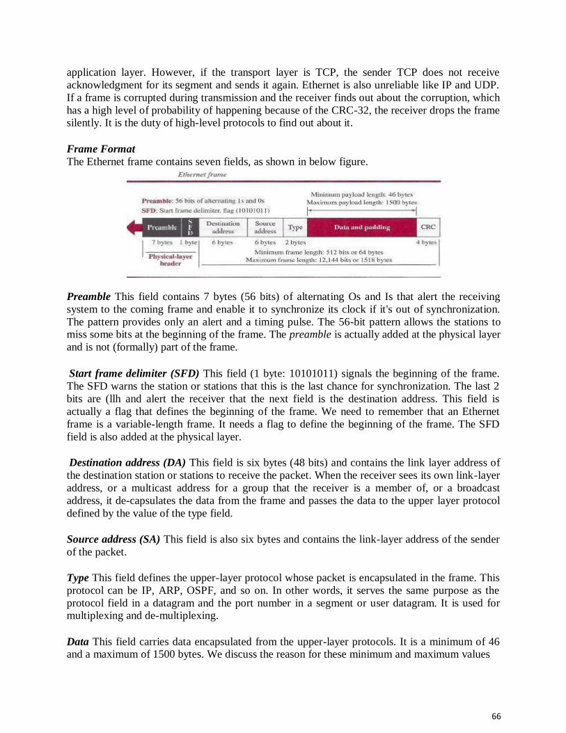
66
application layer. However, if the transport layer is TCP, the sender TCP does not receive
acknowledgment for its segment and sends it again. Ethernet is also unreliable like IP and UDP.
If a frame is corrupted during transmission and the receiver finds out about the corruption, which
has a high level of probability of happening because of the CRC-32, the receiver drops the frame silently. It is the duty of high-level protocols to find out about it.
Frame Format
The Ethernet frame contains seven fields, as shown in below figure.
Preamble This field contains 7 bytes (56 bits) of alternating Os and Is that alert the receiving
system to the coming frame and enable it to synchronize its clock if it's out of synchronization.
The pattern provides only an alert and a timing pulse. The 56-bit pattern allows the stations to miss some bits at the beginning of the frame. The preamble is actually added at the physical layer
and is not (formally) part of the frame.
Start frame delimiter (SFD) This field (1 byte: 10101011) signals the beginning of the frame.
The SFD warns the station or stations that this is the last chance for synchronization. The last 2
bits are (llh and alert the receiver that the next field is the destination address. This field is
actually a flag that defines the beginning of the frame. We need to remember that an Ethernet
frame is a variable-length frame. It needs a flag to define the beginning of the frame. The SFD
field is also added at the physical layer.
Destination address (DA) This field is six bytes (48 bits) and contains the link layer address of
the destination station or stations to receive the packet. When the receiver sees its own link-layer
address, or a multicast address for a group that the receiver is a member of, or a broadcast
address, it de-capsulates the data from the frame and passes the data to the upper layer protocol
defined by the value of the type field.
Source address (SA) This field is also six bytes and contains the link-layer address of the sender
of the packet.
Type This field defines the upper-layer protocol whose packet is encapsulated in the frame. This
protocol can be IP, ARP, OSPF, and so on. In other words, it serves the same purpose as the
protocol field in a datagram and the port number in a segment or user datagram. It is used for multiplexing and de-multiplexing.
Data This field carries data encapsulated from the upper-layer protocols. It is a minimum of 46
and a maximum of 1500 bytes. We discuss the reason for these minimum and maximum values

67
shortly. If the data coming from the upper layer is more than 1500 bytes, it should be fragmented
and encapsulated in more than one frame. If it is less than 46 bytes, it needs to be padded with
extra Os. A padded data frame is delivered to the upper-layer protocol as it is (without removing
the padding), which means that it is the responsibility of the upper layer to remove or, in the case
of the sender, to add the padding. The upper-layer protocol needs to know the length of its data.
For example, a datagram has a field that defines the length of the data.
CRC The last field contains error detection information, in this case a CRC-32. The CRC is calculated over the addresses, types, and data field. If the receiver calculates the CRC and finds
that it is not zero (corruption in transmission), it discards the frame.
Frame Length Ethernet has imposed restrictions on both the minimum and maximum lengths of a frame. The
minimum length restriction is required for the correct operation of CSMAlCD. An Ethernet
frame needs to have a minimum length of 512 bits or 64 bytes. Part of this length is the header
and the trailer. If we count 18 bytes of header and trailer (6 bytes of source address, 6 bytes of
destination address, 2 bytes of length or type, and 4 bytes of CRC), then the minimum length of
data from the upper layer is 64 - 18 = 46 bytes. If the upper-layer packet is less than 46 bytes,
padding is added to make up the difference.
The standard defines the maximum length of a frame (without preamble and SFD field) as 1518
bytes. If we subtract the 18 bytes of header and trailer, the maximum length of the payload is
1500 bytes. The maximum length restriction has two historical reasons. First, memory was very
expensive when Ethernet was designed; a maximum length restriction helped to reduce the size
of the buffer. Second, the maximum length restriction prevents one station from monopolizing
the shared medium, blocking other stations that have data to send.
Minimum frame length: 64 bytes Maximum frame length: 1518 bytes
Minimum data length: 46 bytes Maximum data length: 1500 bytes
Addressing Each station on an Ethernet network (such as a PC, workstation, or printer) has its own network interface card (NIC). The NIC fits inside the station and provides the station with a link-layer
address. The Ethernet address is 6 bytes (48 bits), normally written in hexadecimal notation, with
a colon between the bytes. For example, the following shows an Ethernet MAC address: 4A:30:10:21:10:1A
Transmission of Address Bits The way the addresses are sent out online is different from the way they are written in hexadecimal notation. The transmission is left to right, byte by byte; however, for each byte, the
least significant bit is sent first and the most significant bit is sent last. This means that the bit
that defines an address as unicast or multicast arrives first at the receiver. This helps the receiver
to immediately know if the packet is unicast or multicast.
Example Show how the address 47:20:IB:2E:08:EE is sent out online.

68
Solution The address is sent left to right, byte by byte; for each byte, it is sent right to left, bit by bit, as shown below: Hexadecimal 47 20 IB 2E 08 EE Binary 01000111 00100000 00011011 00101110 00001000 11101110
Transmitted ~ 11100010 00000100 11011000 01110100 00010000 01110111
Unicast, Multicast, and Broadcast Addresses A source address is always a unicast address-the frame comes from only one station. The
destination address, however, can be unicast, multicast, or broadcast. Below figure shows how to
distinguish a unicast address from a multicast address. If the least significant bit of the first byte
in a destination address is 0, the address is unicast; otherwise, it is multicast. Note that with the
way the bits are transmitted, the unicast/multicast bit is the first bit which is transmitted or
received. The broadcast address is a special case of the multicast address: the recipients are all
the stations on the LAN. A broadcast destination address is forty-eight 1s.
Example Define the type of the following destination addresses: a. 4A:30:10:21:10:1A b. 47:20:IB:2E:08:EE c. FF:FF:FF:FF:FF:FF Solution To find the type of the address, we need to look at the second hexadecimal digit from the left. If it is even, the address is unicast. If it is odd, the address is multicast. If all digits are Fs, the
address is broadcast. Therefore, we have the following: a. This is a unicast address because A in binary is 1010 (even). b. This is a multicast address because 7 in binary is 0111 (odd). c. This is a broadcast address because all digits are Fs in hexadecimal
Distinguish Between Unicast, Multicast, and Broadcast Transmission Standard Ethernet uses a coaxial cable (bus topology) or a set of twisted-pair cables with a hub
(star topology) as shown in Figure. We need to know that transmission in the standard Ethernet
is always broadcast, no matter if the intention is unicast, multicast, or broadcast. In the bus
topology, when station A sends a frame to station B, all stations will receive it. In the star
topology, when station A sends a frame to station B, the hub will receive it. Since the hub is a
passive element, it does not check the destination address of the frame; it regenerates the bits (if
they have been weakened) and sends them to all stations except station A. In fact, it floods the
network with the frame. The question is, then, how the actual unicast, multicast, and broadcast
transmissions are distinguished from each other. The answer is in the way the frames are kept
or dropped.
➢ In a unicast transmission, all stations will receive the frame, the intended recipient keeps and handles the frame; the rest discard it.
➢ In a multicast transmission, all stations will receive the frame, the stations that are members of the group keep and handle it; the rest discard it.

69
➢ In a broadcast transmission, all stations (except the sender) will receive the frame andall
stations (except the sender) keep and handle it.
Access Method Since the network that uses the standard Ethernet protocol is a broadcast network, we need to use
an access method to control access to the sharing medium. The standard Ethernet choose CSMA/CD with l-persistent method.
Let us use a scenario to see how this method works for the Ethernet protocol. 1. Assume station A in above figure has a frame to send to station D. Station A first should
check whether any other station is sending (carrier sense). Station A measures the level of
energy on the medium (for a short period of time, normally less than 100 us). If there is
no signal energy on the medium, it means that no station is sending (or the signal has not
reached station A). Station A interprets this situation as idle medium. It starts sending its
frame. On the other hand, if the signal energy level is not zero, it means that the medium
is being used by another station. Station A continuously monitors the medium until it
becomes idle for 100 us, It then starts sending the frame. However, station A needs to
keep a copy of the frame in its buffer until it is sure that there is no collision. When
station A is sure of this is the subject. 2. The medium sensing does not stop after station A has started sending the frame. Station
A needs to send and receive continuously. Two cases may occur: a. Station A has sent 512 bits and no collision is sensed (the energy level did not go above
the regular energy level), the station then is sure that the frame will go through and stops
sensing the medium. Where does the number 512 bits come from? If we consider the
transmission rate of the Ethernet as 10 Mbps, this means that it takes the station 512/(10
Mbps) = 5l.2 us to send out 512 bits. With the speed of propagation in a cable (2 x 10⁸
meters), the first bit could have gone 10,240 meters (one way) or only 5120 meters (round
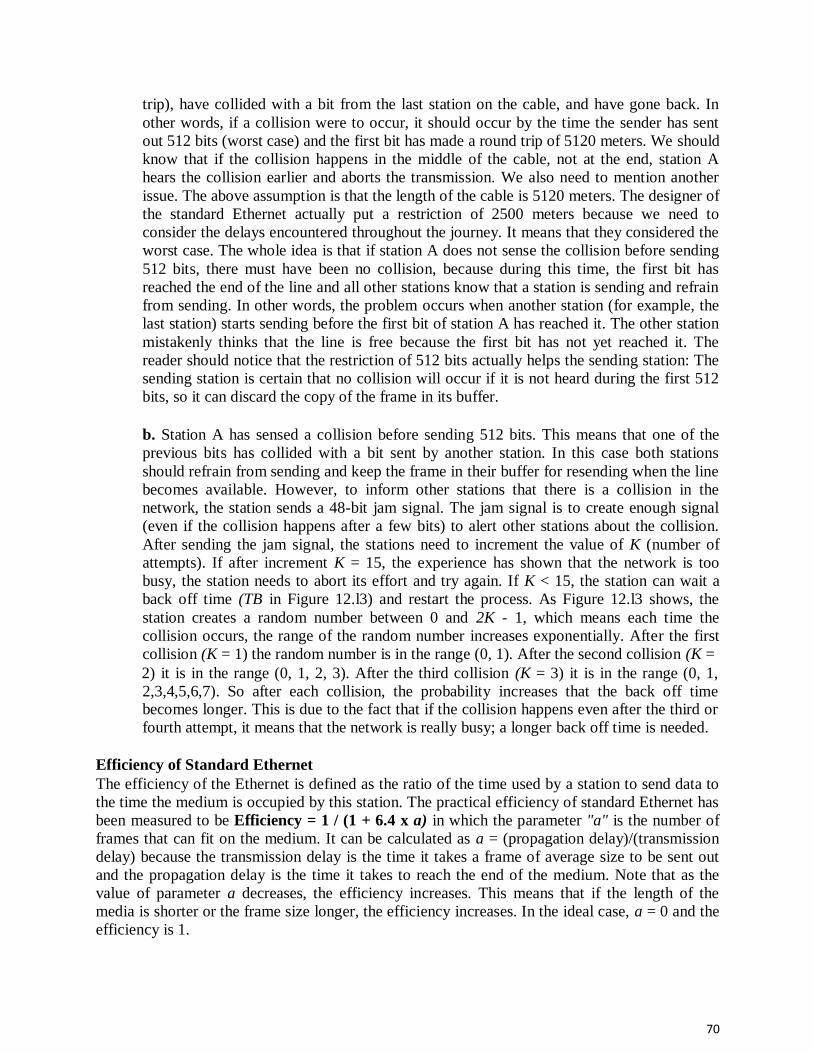
70
trip), have collided with a bit from the last station on the cable, and have gone back. In
other words, if a collision were to occur, it should occur by the time the sender has sent
out 512 bits (worst case) and the first bit has made a round trip of 5120 meters. We should
know that if the collision happens in the middle of the cable, not at the end, station A
hears the collision earlier and aborts the transmission. We also need to mention another
issue. The above assumption is that the length of the cable is 5120 meters. The designer of
the standard Ethernet actually put a restriction of 2500 meters because we need to
consider the delays encountered throughout the journey. It means that they considered the
worst case. The whole idea is that if station A does not sense the collision before sending
512 bits, there must have been no collision, because during this time, the first bit has
reached the end of the line and all other stations know that a station is sending and refrain
from sending. In other words, the problem occurs when another station (for example, the
last station) starts sending before the first bit of station A has reached it. The other station
mistakenly thinks that the line is free because the first bit has not yet reached it. The
reader should notice that the restriction of 512 bits actually helps the sending station: The
sending station is certain that no collision will occur if it is not heard during the first 512
bits, so it can discard the copy of the frame in its buffer.
b. Station A has sensed a collision before sending 512 bits. This means that one of the
previous bits has collided with a bit sent by another station. In this case both stations
should refrain from sending and keep the frame in their buffer for resending when the line
becomes available. However, to inform other stations that there is a collision in the
network, the station sends a 48-bit jam signal. The jam signal is to create enough signal
(even if the collision happens after a few bits) to alert other stations about the collision.
After sending the jam signal, the stations need to increment the value of K (number of
attempts). If after increment K = 15, the experience has shown that the network is too
busy, the station needs to abort its effort and try again. If K < 15, the station can wait a
back off time (TB in Figure 12.l3) and restart the process. As Figure 12.l3 shows, the
station creates a random number between 0 and 2K - 1, which means each time the
collision occurs, the range of the random number increases exponentially. After the first
collision (K = 1) the random number is in the range (0, 1). After the second collision (K = 2) it is in the range (0, 1, 2, 3). After the third collision (K = 3) it is in the range (0, 1,
2,3,4,5,6,7). So after each collision, the probability increases that the back off time becomes longer. This is due to the fact that if the collision happens even after the third or
fourth attempt, it means that the network is really busy; a longer back off time is needed.
Efficiency of Standard Ethernet The efficiency of the Ethernet is defined as the ratio of the time used by a station to send data to
the time the medium is occupied by this station. The practical efficiency of standard Ethernet has
been measured to be Efficiency = 1 / (1 + 6.4 x a) in which the parameter "a" is the number of
frames that can fit on the medium. It can be calculated as a = (propagation delay)/(transmission
delay) because the transmission delay is the time it takes a frame of average size to be sent out
and the propagation delay is the time it takes to reach the end of the medium. Note that as the
value of parameter a decreases, the efficiency increases. This means that if the length of the
media is shorter or the frame size longer, the efficiency increases. In the ideal case, a = 0 and the
efficiency is 1.

71
Example In the Standard Ethernet with the transmission rate of 10 Mbps, we assume that the length of the medium is 2500 m and the size of the frame is 512 bits. The propagation speed of a signal in a
cable is normally 2 x 10⁸ mls. Propagation delay = 2500/ (2 x 10⁸) = 12.5 fJ.s Transmission
delay = 512/ (107) = 51.2 fJ.S a = 12.5/51.2 = 0.24 Efficiency = 39%
The example shows that a = 0.24, which means only 0.24 of a frame occupies the whole medium
in this case. The efficiency is 39 percent, which is considered moderate; it means that only 61 percent of the time the medium is occupied but not used by a station.
Implementation The Standard Ethernet defined several implementations, but only four of them became popular during the 1980s. Table shows a summary of Standard Ethernet implementations. Table
In the nomenclature 10BaseX, the number defines the data rate (10 Mbps), the term Base means
baseband (digital) signal, and X approximately defines either the maximum size of the cable in
100 meters (for example 5 for 500 or 2 for 185 meters) or the type of cable, T for unshielded
twisted pair cable (UTP) and F for fiber-optic. The standard Ethernet uses a baseband signal,
which means that the bits are changed to a digital signal and directly sent on the line.
Encoding and Decoding All standard implementations use digital signaling (baseband) at 10 Mbps. At the sender, data are
converted to a digital signal using the Manchester scheme; at the receiver, the received signal is interpreted as Manchester and decoded into data. Manchester encoding is self-synchronous,
providing a transition at each bit interval. Figure shows the encoding scheme for Standard
Ethernet.

72
10BaseS: Thick Ethernet The first implementation is called 1OBaseS, thick Ethernet, or Thicknet. The nickname derives
from the size of the cable, which is roughly the size of a garden hose and too stiff to bend with your hands. 10Base5 was the first Ethernet specification to use a bus topology with an external
transceiver (transmitter/receiver) connected via a tap to a thick coaxial cable. Figure shows a
schematic diagram of a 10Base5 implementation.
The transceiver is responsible for transmitting, receiving, and detecting collisions. The
transceiver is connected to the station via a transceiver cable that provides separate paths for
sending and receiving. This means that collision can only happen in the coaxial cable. The
maximum length of the coaxial cable must not exceed 500 m, otherwise, there is excessive
degradation of the signal. If a length of more than 500 m is needed, up to five segments, each a
maximum of 500 meters, can be connected using repeaters.
10Base2: Thin Ethernet The second implementation is called lOBase2, thin Ethernet, or Cheaper net. lOBase2 also uses a
bus topology, but the cable is much thinner and more flexible. The cable can be bent to pass very
close to the stations. In this case, the transceiver is normally part of the network interface card
(NIC), which is installed inside the station. Figure shows the schematic diagram of a 10Base2 implementation.

73
Note that the collision here occurs in the thin coaxial cable. This implementation is more cost
effective than 10Base5 because thin coaxial cable is less expensive than thick coaxial and the tee
connections are much cheaper than taps. Installation is simpler because the thin coaxial cable is
very flexible. However, the length of each segment cannot exceed 185 m (close to 200 m) due to the high level of attenuation in thin coaxial cable.
10Base-T: Twisted-Pair Ethernet The third implementation is called 1OBase- T or twisted-pair Ethernet. 1OBase-T uses a physical star topology. The stations are connected to a hub via two pairs of twisted cable, as
shown in Figure.
Note that two pairs of twisted cable create two paths (one for sending and one for receiving)
between the station and the hub. Any collision here happens in the hub. Compared to lOBase5 or
lOBase2, we can see that the hub actually replaces the coaxial cable as far as a collision is
concerned. The maximum length of the twisted cable here is defined as 100 m, to minimize the effect of attenuation in the twisted cable.
10Base-F: Fiber Ethernet Although there are several types of optical fiber 10-Mbps Ethernet, the most common is called lOBase-F. 1OBase-F uses a star topology to connect stations to a hub. The stations are connected
to the hub using two fiber-optic cables, as shown in Figure.
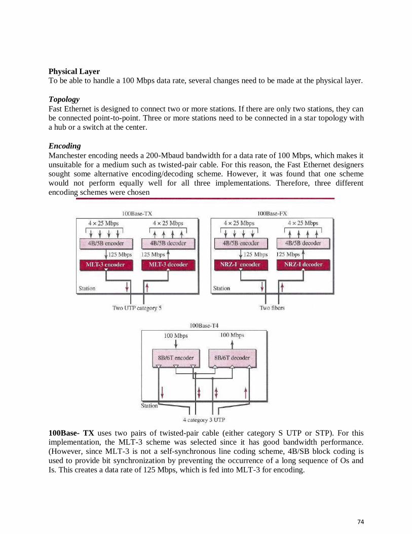
74
Physical Layer
To be able to handle a 100 Mbps data rate, several changes need to be made at the physical layer.
Topology Fast Ethernet is designed to connect two or more stations. If there are only two stations, they can be connected point-to-point. Three or more stations need to be connected in a star topology with
a hub or a switch at the center.
Encoding Manchester encoding needs a 200-Mbaud bandwidth for a data rate of 100 Mbps, which makes it
unsuitable for a medium such as twisted-pair cable. For this reason, the Fast Ethernet designers sought some alternative encoding/decoding scheme. However, it was found that one scheme
would not perform equally well for all three implementations. Therefore, three different
encoding schemes were chosen
100Base- TX uses two pairs of twisted-pair cable (either category S UTP or STP). For this
implementation, the MLT-3 scheme was selected since it has good bandwidth performance.
(However, since MLT-3 is not a self-synchronous line coding scheme, 4B/SB block coding is
used to provide bit synchronization by preventing the occurrence of a long sequence of Os and
Is. This creates a data rate of 125 Mbps, which is fed into MLT-3 for encoding.
75
100Base-FX uses two pairs of fiber-optic cables. Optical fiber can easily handle high bandwidth
requirements by using simple encoding schemes. The designers of 100Base-FX selected the
NRZ-I encoding scheme for this implementation. However, NRZ-I has a bit synchronization
problem for long sequences of 0s (or Is, based on the encoding). To overcome this problem, the
designers used 4B/5B block encoding, as we described for 100Base- TX. The block encoding
increases the bit rate from 100 to 125 Mbps, which can easily be handled by fiber-optic cable. A
100Base-TX network can provide a data rate of 100 Mbps, but it requires the use of category 5
UTP or STP cable. This is not cost-efficient for buildings that have already been wired for voice-
grade twisted-pair (category 3). A new standard, called lOOBase-T4, was designed to use
category 3 or higher UTP. The implementation uses four pairs of UTP for transmitting 100
Mbps. Encoding/decoding in 100Base-T4 is more complicated. As this implementation uses
category 3 UTP, each twisted-pair cannot easily handle more than 25 Mbaud. In this design, one
pair switches between sending and receiving. Three pairs of UTP category 3, however, can
handle only 75 Mbaud (25 Mbaud) each. We need to use an encoding scheme that converts 100
Mbps to a 75 Mbaud signal. 8B/6T satisfies this requirement. In 8B/6T, eight data elements are
encoded as six signal elements. This means that 100 Mbps uses only (6/8) x 100 Mbps, or 75
Mbaud.
MAC Sublayer A main consideration in the evolution of Ethernet was to keep the MAC sub layer untouched. However, to achieve a data rate of 1 Gbps, this was no longer possible. Gigabit Ethernet has two
distinctive approaches for medium access: half-duplex and full duplex. Almost all
implementations of Gigabit Ethernet follow the full-duplex approach, so we mostly ignore the
half-duplex mode.
Full-Duplex Mode In full-duplex mode, there is a central switch connected to all computers or other switches. In this
mode, for each input port, each switch has buffers in which data are stored until they are
transmitted. Since the switch uses the destination address of the frame and sends a frame out of
the port connected to that particular destination, there is no collision. This means that CSMA/CD
is not used. Lack of collision implies that the maximum length of the cable is determined by the
signal attenuation in the cable, not by the collision detection process. In the full-duplex mode of
Gigabit Ethernet, there is-no collision; the maximum length of the cable is determined by the
signal attenuation in the cable.
Half-Duplex Mode Gigabit Ethernet can also be used in half-duplex mode, although it is rare. In this case, a switch can be replaced by a hub, which acts as the common cable in which a collision might occur. The
half-duplex approach uses CSMA/CD. However, as we saw before, the maximum length of the
network in this approach is totally dependent on the minimum frame size. Three methods have
been defined: traditional, carrier extension, and frame bursting.
Traditional In the traditional approach, we keep the minimum length of the frame as in traditional Ethernet
(512 bits). However, because the length of a bit is 1/100 shorter in Gigabit Ethernet than in 10-Mbps Ethernet, the slot time for Gigabit Ethernet is 512 bits x 11 1000 us, which is equal to

76
0.512 J.lS. The reduced slot time means that collision is detected 100 times earlier. This means
that the maximum length of the network is 25 m. This length may be suitable if all the stations
are in one room, but it may not even be long enough to connect the computers in one single
office.
Carrier Extension To allow for a longer network, we increase the minimum frame length. The carrier extension
approach defines the minimum length of a frame as 512 bytes (4096 bits). This means that the
minimum length is 8 times longer. This method forces a station to add extension bits (padding) to
any frame that is less than 4096 bits. In this way, the maximum length of the network can be
increased 8 times to a length of 200 m. This allows a length of 100 m from the hub to the station.
Frame Bursting Carrier extension is very inefficient if we have a series of short frames to send; each frame arries
redundant data. To improve efficiency, frame bursting was proposed. Instead of adding an
extension to each frame, multiple frames are sent. However, to make these multiple frames look
like one frame, padding is added between the frames (the same as that used for the carrier
extension method) so that the channel is not idle. In other words, the method deceives other
stations into thinking that a very large frame has been transmitted.
Physical Layer The physical layer in Gigabit Ethernet is more complicated than that in Standard or Fast Ethernet. We briefly discuss some features of this layer.
Topology Gigabit Ethernet is designed to connect two or more stations. If there are only two stations, they
can be connected point-to-point. Three or more stations need to be connected in a star topology
with a hub or a switch at the center. Another possible configuration is to connect several star
topologies or let one star topology be part of another.
Implementation Gigabit Ethernet can be categorized as either a two-wire or a four-wire implementation. The two-
wire implementations use fiber-optic cable (l000Base-SX, short-wave, or l000Base-LX, long-
wave), or STP (l000Base-CX). The four-wire version uses category 5 twisted-pair cable
(l000Base-T). In other words, we have four implementations. 1000Base-T was designed in
response to those users who had already installed this wiring for other purposes such as Fast
Ethernet or telephone services.
Encoding Figure shows the encoding/decoding schemes for the four implementations. Gigabit Ethernet
cannot use the Manchester encoding scheme because it involves a very high bandwidth (2
GBaud). The two-wire implementations use an NRZ scheme, but NRZ does not self-synchronize
properly. To synchronize bits, particularly at this high data rate, SBIl0B block encoding,
discussed in Chapter 4, is used. This block encoding prevents long sequences of 0s or Is in the
stream, but the resulting stream is 1.25 Gbps. Note that in this implementation, one wire (fiber or
STP) is used for sending and one for receiving. In the four-wire implementation it is not possible

77
to have 2 wires for input and 2 for output, because each wire would need to carry 500 Mbps,
which exceeds the capacity for category 5 UTP. Thus, all four wires are involved in both input
and output; each wire carries 250 Mbps, which is in the range for category 5 UTP cable.
DATA LINK LAYER SWITCHING Many organizations have multiple LANs and wish to connect them. Would it not be convenient
if we could just join the LANs together to make a larger LAN? In fact, we can do this when the
connections are made with devices called bridges. are a modern name for bridges; they provide functionality that goes beyond classic Ethernet and Ethernet hubs to make it easy to join multiple
LANs into a larger and faster network.
We shall use the terms ‘‘bridge’’ and ‘‘switch’’ interchangeably. Bridges operate in the data link
layer, so they examine the data link layer addresses to forward frames. Since they are not
supposed to examine the payload field of the frames they forward, they can handle IP packets as
well as other kinds of packets, such as AppleTalk packets. In contrast, routers examine the
addresses in packets and route based on them, so they only work with the protocols that they
were designed to handle. physical LANs into a single logical LAN. We will also look at how to
do the reverse and treat one physical LAN as multiple logical LANs, called VLANs (Virtual
LANs). Both technologies provide useful flexibility for managing networks. For a
comprehensive treatment of bridges, switches, and related topics, see Seifert and Edwards (2008)
and Perlman (2000).
Uses of Bridges Before getting into the technology of bridges, let us take a look at some common situations in which bridges are used. We will mention three reasons why a single organization may end up
with multiple LANs. First, many university and corporate departments have their own LANs to connect their own personal computers, servers, and devices such as printers. Since the goals of the various
78
departments differ, different departments may set up different LANs, without regard to what
other departments are doing. Sooner or later, though, there is a need for interaction, so bridges
are needed. In this example, multiple LANs come into existence due to the autonomy of their
owners.
Second, the organization may be geographically spread over several buildings separated by
considerable distances. It may be cheaper to have separate LANs in each building and connect
them with bridges and a few long-distance fiber optic links than to run all the cables to a single
central switch. Even if laying the cables is easy to do, there are limits on their lengths (e.g., 200
m for twisted-pair gigabit Ethernet). The network would not work for longer cables due to the
excessive signal attenuation or round-trip delay. The only solution is to partition the LAN and
install bridges to join the pieces to increase the total physical distance that can be covered.
Third, it may be necessary to split what is logically a single LAN into separate LANs (connected
by bridges) to accommodate the load. At many large universities, for example, thousands of
workstations are available for student and faculty computing. Companies may also have
thousands of employees. The scale of this system precludes putting all the workstations on a
single LAN—there are more computers than ports on any Ethernet hub and more stations than
allowed on a single classic Ethernet.
Even if it were possible to wire all the workstations together, putting more stations on an
Ethernet hub or classic Ethernet would not add capacity. All of the stations share the same, fixed
amount of bandwidth. The more stations there are, the less average bandwidth per station.
However, two separate LANs have twice the capacity of a single LAN. Bridges let the LANs be
joined together while keeping this capacity. The key is not to send traffic onto ports where it is
not needed, so that each LAN can run at full speed. This behavior also increases reliability, since
on a single LAN a defective node that keeps outputting a continuous stream of garbage can clog
up the entire LAN. By deciding what to forward and what not to forward, bridges act like fire
doors in a building, preventing a single node that has gone berserk from bringing down the entire
system. To make these benefits easily available, ideally bridges should be completely
transparent. It should be possible to go out and buy bridges, plug the LAN cables into the
bridges, and have everything work perfectly, instantly. There should be no hardware changes
required, no software changes required, no setting of address switches, no downloading of
routing tables or parameters, nothing at all. Just plug in the cables and walk away. Furthermore,
the operation of the existing LANs should not be affected by the bridges at all. As far as the
stations are concerned, there should be no observable difference whether or not they are part of a
bridged LAN. It should be as easy to move stations around the bridged LAN as it is to move
them around a single LAN.
Surprisingly enough, it is actually possible to create bridges that are transparent. Two algorithms
are used: a backward learning algorithm to stop traffic being sent where it is not needed; and a
spanning tree algorithm to break loops that may be formed when switches are cabled together
willy-nilly. Let us now take a Learning Bridges The topology of two LANs bridged together is shown in
figure. On the left-hand side, two multidrop LANs, such as classic Ethernets, are joined by a special station—the bridge—that sits on both LANs. On the right-hand side, LANs with point-to-

79
point cables, including one hub, are joined together. The bridges are the devices to which the
stations and hub are attached. If the LAN technology is Ethernet, the bridges are better known as
Ethernet switches.
(a) Bridge connecting two multidrop LANs. (b) Bridges (and a hub) connecting seven point-to-
point stations
Bridges were developed when classic Ethernets were in use, so they are often shown in
topologies with multidrop cables, as in Fig. 4-41(a). However, all the topologies that are
encountered today are comprised of point-to-point cables and switches. The bridges work the
same way in both settings. All of the stations attached to the same port on a bridge belong to the
same collision domain, and this is different than the collision domain for other ports. If there is
more than one station, as in a classic Ethernet, a hub, or a half-duplex link, the CSMA/CD
protocol is used to send frames.
There is a difference, however, in how the bridged LANs are built. To bridge multidrop LANs, a
bridge is added as a new station on each of the multidrop LANs, as in Fig. 4-41(a). To bridge
point-to-point LANs, the hubs are either connected to a bridge or, preferably, replaced with a
bridge to increase performance. In Fig. bridges have replaced all but one hub. Different kinds of
cables can also be attached to one bridge. For example, the cable connecting bridge B1 to bridge
B2 in Fig. might be a long-distance fiber optic link, while the cable connecting the bridges to
stations might be a short-haul twisted-pair line. This arrangement is useful for bridging LANs in
different buildings.
Now let us consider what happens inside the bridges. Each bridge operates in promiscuous mode, that is, it accepts every frame transmitted by the stations attached to each of its ports. The bridge
must decide whether to forward or discard each frame, and, if the former, on which port to output
the frame. This decision is made by using the destination address. As an example, consider the
topology of Fig. If station A sends a frame to station B, bridge B1 will receive the frame on port 1. This frame can be immediately discarded without further ado because it is already on the correct port. However, in the topology of Fig. suppose that A sends a frame to D. Bridge B1 will
receive the frame on port 1 and output it on port 4. Bridge B2 will then receive the frame on its
port 4 and output it on its port 1.
A simple way to implement this scheme is to have a big (hash) table inside the bridge. The table
can list each possible destination and which output port it belongs on. For example, in Fig, the
table at B1 would list D as belonging to port 4, since all B1 has to know is which port to put frames on to reach D. That, in fact, more forwarding will happen later when the frame hits B2 is
not of interest to B1..

80
As mentioned above, the bridges operate in promiscuous mode, so they see every frame sent on
any of their ports. By looking at the source addresses, they can tell which machines are
accessible on which ports. For example, if bridge B1 in Fig sees a frame on port 3 coming from
C, it knows that C must be reachable via port 3, so it makes an entry in its hash table. Any
subsequent frame addressed to C coming in to B1 on any other port will be forwarded to port
3.The topology can change as machines and bridges are powered up and down and moved
around. To handle dynamic topologies, whenever a hash table entry is made, the arrival time of
the frame is noted in the entry. Whenever a frame whose source is already in the table arrives,
its entry is updated with the current time. Thus, the time associated with every entry tells the
last time a frame from that machine was seen. Periodically, a process in the bridge scans the
hash table and purges all entries more than a few minutes old. In this way, if a computer is
unplugged from its LAN, moved around the building, and plugged in again somewhere else,
within a few minutes it will be back in normal operation, without any manual intervention. This
algorithm also means that if a machine is quiet for a few minutes, any traffic sent to it will have
to be flooded until it next sends a frame itself. The routing procedure for an incoming frame
depends on the port it arrives on (the source port) and the address to which it is destined (the
destination address).
The procedure is as follows:
1. If the port for the destination address is the same as the source port, discard the frame. 2. If the port for the destination address and the source port are different, forward the frame on to the destination port. 3. If the destination port is unknown, use flooding and send the frame on all ports except the source port.
You might wonder whether the first case can occur with point-to-point links. The answer is that it
can occur if hubs are used to connect a group of computers to a bridge. An example is shown in
Fig. 4-41(b) where stations E and F are connected to hub H1, which is in turn connected to
bridge B2. If E sends a frame to F, the hub will relay it to B2 as well as to F. That is what hubs
do—they wire all ports together so that a frame input on one port is simply output on all other
ports. The frame will arrive at B2 on port 4, which is already the right output port to reach the
destination. Bridge B2 need only discard the frame. As each frame arrives, this algorithm must be
applied, so it is usually implemented with special-purpose VLSI chips.
The chips do the lookup and update the table entry, all in a few microseconds. Because bridges
only look at the MAC addresses to decide how to forward frames, it is possible to start
forwarding as soon as the destination header field has come in, before the rest of the frame has
arrived (provided the output line is available, of course). This design reduces the latency of
passing through the bridge, as well as the number of frames that the bridge must be able to
buffer. It is referred to as cut-through switching or wormhole routing and is usually handled in
hardware. We can look at the operation of a bridge in terms of protocol stacks to understand what
it means to be a link layer device. Consider a frame sent from station A to station D in the
configuration of Fig), in which the LANs are Ethernet. The frame will pass through one bridge.
The protocol stack view of processing is shown in Fig .The packet comes from a higher layer and
descends into the Ethernet MAC layer. It acquires an Ethernet header (and also a trailer, not
shown in the figure). This unit is passed to the physical layer, goes out over the cable, and is

81
picked up by the bridge. In the bridge, the frame is passed up from the physical layer to the
Ethernet MAC layer. This layer has extended processing compared to the Ethernet MAC layer at
a station. It passes the frame to a relay, still within the MAC layer. The bridge relay function
uses only the Ethernet MAC header to determine how to handle the frame. In this case, it passes
the frame to the Ethernet MAC layer of the port used to reach station D, and the frame continues
on its way. In the general case, relays at a given layer can rewrite the headers for that layer.
VLANs will provide an example shortly. In no case should the bridge look inside the frame and
learn that it is carrying an IP packet; that is irrelevant to the
bridge processing and would violate protocol layering. Also note that a bridge with k ports will have k instances of MAC and physical layers. The value of k is 2 for our simple example.
Spanning Tree Bridges To increase reliability, redundant links can be used between bridges. In the example of Fig,
there are two links in parallel between a pair of bridges. This design ensures that if one link is cut, the network will not be partitioned into two sets of computers that cannot talk to each other.
However, this redundancy introduces some additional problems because it creates loops in the
topology. An example of these problems can be seen by looking at how a frame sent by A to a
previously unobserved destination is handled in Fig.. Each bridge follows the normal rule for
handling unknown destinations, which is to flood the frame. Call the frame from A that reaches
bridge B1 frame F0. The bridge sends copies of this frame out all of its other ports. We will only
consider the bridge ports that connect B1 to B2 (though the frame will be sent out the other ports,
too). Since there are two links from B1 to B2, two copies of the frame will reach B2. They are
shown in Fig as F1 and F2. Shortly thereafter, bridge B2 receives these frames. However, it does
not (and cannot) know that they are copies of the same frame, rather than two different frames
sent one after the other. So bridge B2 takes F1 and sends copies of it out all the other ports, and it
also takes F2 and sends copies of it out all the other ports. This produces frames F3 and F4 that
are sent along the two links back to B1. Bridge B1 then sees two new frames with unknown
destinations and copies them again. This cycle goes on forever. The solution to this difficulty is
for the bridges to communicate with each other and overlay the actual topology with a spanning

82
tree that reaches every bridge. In effect, some potential connections between bridges are ignored
in the interest of constructing a fictitious loop-free topology that is a subset of the actual topology.
For example, in Fig. we see five bridges that are interconnected and also have stations connected
to them. Each station connects to only one bridge. There are some redundant connections
between the bridges so that frames will be forwarded in loops if all of the links are used. This
topology can be thought of as a graph in which the bridges are the nodes and the point-to-point
links are the edges. The graph can be reduced to a spanning tree, which has no cycles by
definition, by dropping the links shown as dashed lines in Fig. Using this spanning tree, there is
exactly one path from every station to every other station. Once the bridges have agreed on the
spanning tree, all forwarding between stations follows the spanning tree. Since there is a unique
path from each source to each destination, loops are impossible.
To build the spanning tree, the bridges run a distributed algorithm. Each bridge periodically
broadcasts a configuration message out all of its ports to it neighbors and processes the messages
it receives from other bridges, as described next. These messages are not forwarded, since their
purpose is to build the tree, which can then be used for forwarding. The bridges must first choose
one bridge to be the root of the spanning tree. To make this choice, they each include an
identifier based on their MAC address in the configuration message, as well as the identifier of
the bridge they believe to be the root. MAC addresses are installed by the manufacturer and
guaranteed to be unique worldwide, which makes these identifiers convenient and unique. The
bridges choose the bridge with the lowest identifier to be the root. After enough messages have
been exchanged to spread the news, all bridges will agree on which bridge is the root. In Fig.,
bridge B1 has the lowest identifier and becomes the root. Next, a tree of shortest paths from the
root to every bridge is constructed. In Fig. bridges B2 and B3 can each be reached from bridge
B1 directly, in one hop that is a shortest path. Bridge B4 can be reached in two hops, via either
B2 or B3. To break this tie, the path via the bridge with the lowest identifier is chosen, so B4 is
reached via B2. Bridge B5 can be reached in two hops via B3. To find these shortest paths,
bridges include the distance from the root in their configuration messages. Each bridge
remembers the shortest path it finds to the root. The bridges then turn off ports that are not part of
the shortest path. Although the tree spans all the bridges, not all the links (or even bridges) are
necessarily present in the tree. This happens because turning off the ports prunes some links from
the network to prevent loops. Even after the spanning tree has been established, the algorithm
continues to run during normal operation to automatically detect topology changes and update
the tree.

83
The algorithm for constructing the spanning tree was invented by Radia Perlman. Her job was to
solve the problem of joining LANs without loops. She was given a week to do it, but she came
up with the idea for the spanning tree algorithm in a day. Fortunately, this left her enough time to
write it as a poem (Perlman, 1985): The spanning tree algorithm was then standardized as IEEE 802.1D and used for many years. In 2001, it was revised to more rapidly find a new spanning tree after a topology change. For a
detailed treatment of bridges, see Perlman (2000).
Repeaters, Hubs, Bridges, Switches, Routers, and Gateways The key to understanding these devices is to realize that they operate in different layers, as
illustrated in Fig. 4-45(a). The layer matters because different devices use different pieces of
information to decide how to switch. In a typical scenario, the user generates some data to be
sent to a remote machine. Those data are passed to the transport layer, which then adds a header
(for example, a TCP header) and passes the resulting unit down to the network layer. The
network layer adds its own header to form a network layer packet (e.g., an IP packet). In Fig. we
see the IP packet shaded in gray. Then the packet goes to the data link layer, which adds its own
header and checksum (CRC) and gives the resulting frame to the physical layer for transmission,
for example, over a LAN.
Now let us look at the switching devices and see how they relate to the packets and frames. At the bottom, in the physical layer, we find the repeaters. These are analog devices that work with
signals on the cables to which they are connected. A signal appearing on one cable is cleaned up,
amplified, and put out on another cable. Repeaters do not understand frames, packets, or headers.
They understand the symbols that encode bits as volts. Classic Ethernet, for example, was
designed to allow four repeaters that would boost the signal to extend the maximum cable length from 500 meters to 2500 meters. Next we come to the hubs. A hub has a number of input lines
that it joins electrically. Frames arriving on any of the lines are sent out on all the others. If two
frames arrive at the same time, they will collide, just as on a coaxial cable. All the lines coming
into a hub must operate at the same speed. Hubs differ from repeaters in that they do not (usually) amplify the incoming signals and are designed for multiple input lines, but the
differences are slight. Like repeaters, hubs are physical layer devices that do not examine the link
layer addresses or use them in any way.
Now let us move up to the data link layer, where we find bridges and switches. We just studied
bridges at some length. A bridge connects two or more LANs. Like a hub, a modern bridge has
multiple ports, usually enough for 4 to 48 input lines of a certain type. Unlike in a hub, each port
is isolated to be its own collision domain; if the port has a full-duplex point-to-point line, the

84
CSMA/CD algorithm is not needed. When a frame arrives, the bridge extracts the destination
address from the frame header and looks it up in a table to see where to send the frame. For
Ethernet, this address is the 48-bit destination address shown in Fig. The bridge only outputs the
frame on the port where it is needed and can forward multiple frames at the same time.
Bridges offer much better performance than hubs, and the isolation between bridge ports also
means that the input lines may run at different speeds, possibly even with different network
types. A common example is a bridge with ports that connect to 10-, 100-, and 1000-Mbps
Ethernet. Buffering within the bridge is needed to accept a frame on one port and transmit the
frame out on a different port. If frames come in faster than they can be retransmitted, the bridge
may run out of buffer space and have to start discarding frames. For example, if a gigabit
Ethernet is pouring bits into a 10-Mbps Ethernet at top speed, the bridge will have to buffer them,
hoping not to run out of memory. This problem still exists even if all the ports run at the same
speed because more than one port may be sending frames to a given destination port.
Bridges were originally intended to be able to join different kinds of LANs, for example, an
Ethernet and a Token Ring LAN. However, this never worked well because of differences
between the LANs. Different frame formats require copying and reformatting, which takes CPU
time, requires a new checksum calculation, and introduces the possibility of undetected errors
due to bad bits in the bridge’s memory. Different maximum frame lengths are also a serious
problem with no good solution. Basically, frames that are too large to be forwarded must be
discarded. So much for transparency.
Two other areas where LANs can differ are security and quality of service. Some LANs have
link-layer encryption, for example 802.11, and some do not, for example Ethernet. Some LANs
have quality of service features such as priorities, for example 802.11, and some do not, for
example Ethernet. Consequently, when a frame must travel between these LANs, the security or
quality of service expected by the sender may not be able to be provided. For all of these reasons,
modern bridges usually work for one network type, and routers, which we will come to soon, are
used instead to join networks of different types. Switches are modern bridges by another name.
The differences are more to do with marketing than technical issues, but there are a few points worth knowing.
Bridges were developed when classic Ethernet was in use, so they tend to join relatively few
LANs and thus have relatively few ports. The term ‘‘switch’’ is more popular nowadays. Also,
modern installations all use point-to-point links, such as twisted-pair cables, so individual
computers plug directly into a switch and thus the switch will tend to have many ports. Finally,
‘‘switch’’ is also used as a general term. With a bridge, the functionality is clear. On the other
hand, a switch may refer to an Ethernet switch or a completely different kind of device that
makes forwarding decisions, such as a telephone switch. So far, we have seen repeaters and hubs,
which are actually quite similar, as well as bridges and switches, which are even more similar to
each other. Now we move up to routers, which are different from all of the above. When a packet
comes into a router, the frame header and trailer are stripped off and the packet located in the
frame’s payload field is passed to the routing software. This software uses the packet header to
choose an output line. For an IP packet, the packet header will contain a 32-bit (IPv4) or 128-bit
(IPv6) address, but not a 48-bit IEEE 802 address. The routing software does not see the frame
addresses and does not even know whether the packet came in on a LAN or a point-to-point line.

85
Up another layer, we find transport gateways. These connect two computers that use different
connection-oriented transport protocols. For example, suppose a computer using the connection-
oriented TCP/IP protocol needs to talk to a computer using a different connection-oriented
transport protocol called SCTP. The transport gateway can copy the packets from one connection
to the other, reformatting them as need be.
Finally, application gateways understand the format and contents of the data and can translate
messages from one format to another. An email gateway could translate Internet messages into SMS messages for mobile phones, for example. Like ‘‘switch,’’ ‘‘gateway’’ is somewhat of a
general term. It refers to a forwarding process that runs at a high layer.

86
UNIT – III
Network Layer
NETWORK LAYER DESIGN ISSUES In the following sections, we will give an introduction to some of the issues that the designers of the network layer must grapple with. These issues include the service provided to the transport
layer and the internal design of the network.
Store-and-Forward Packet Switching
Before starting to explain the details of the network layer, it is worth restating the context in
which the network layer protocols operate. This context can be seen in. The major components of
the network are the ISP’s equipment (routers connected by transmission lines), shown inside the
shaded oval, and the customers’ equipment, shown outside the oval. Host H1 is directly
connected to one of the ISP’s routers, A, perhaps as a home computer that is plugged into a DSL
modem. In contrast, H2 is on a LAN, which might be an office Ethernet, with a router, F, owned
and operated by the customer. This router has a leased line to the ISP’s equipment. We have
shown F as being outside the oval because it does not belong to the ISP. For the purposes of this
chapter, however, routers on customer premises are considered part of the ISP network because
they run the same algorithms as the ISP’s routers (and our main concern here is algorithms).
The environment of the network layer protocols. This equipment is used as follows. A host with a packet to send transmits it to the nearest router,
either on its own LAN or over a point-to-point link to the ISP. The packet is stored there until it has fully arrived and the link has finished its processing by verifying the checksum. Then it is
forwarded to the next router along the path until it reaches the destination host, where it is
delivered. This mechanism is store-and-forward packet switching.
Services Provided to the Transport Layer The network layer provides services to the transport layer at the network layer/transport layer
interface. An important question is precisely what kind of services the network layer provides to the transport layer. The services need to be carefully designed with the following goals in mind: 1. The services should be independent of the router technology. 2. The transport layer should be shielded from the number, type, and topology of the routers present.

87
3. The network addresses made available to the transport layer should use a uniform numbering plan, even across LANs and WANs. Given these goals, the designers of the network layer have a lot of freedom in writing detailed
specifications of the services to be offered to the transport layer. This freedom often degenerates into a raging battle between two warring factions. The discussion
centers on whether the network layer should provide connection-oriented service or connectionless service.
One camp (represented by the Internet community) argues that the routers’ job is moving packets
around and nothing else. In this view (based on 40 years of experience with a real computer
network), the network is inherently unreliable, no matter how it is designed. Therefore, the hosts
should accept this fact and do error control (i.e., error detection and correction) and flow control
themselves. This viewpoint leads to the conclusion that the network service should be
connectionless, with primitives SEND PACKET and RECEIVE PACKET and little else. In
particular, no packet ordering and flow control should be done, because the hosts are going to do
that anyway and there is usually little to be gained by doing it twice. This reasoning is an
example of the end-to-end argument, a design principle that has been very influential in shaping
the Internet (Saltzer et al., 1984). Furthermore, each packet must carry the full destination
address, because each packet sent is carried independently of its predecessors, if any.
The other camp (represented by the telephone companies) argues that the network should provide
a reliable, connection-oriented service. They claim that 100 years of successful experience with
the worldwide telephone system is an excellent guide. In this view, quality of service is the
dominant factor, and without connections in the network, quality of service is very difficult to
achieve, especially for real-time traffic such as voice and video. Even after several decades, this
controversy is still very much alive. Early, widely used data networks, such as X.25 in the 1970s
and its successor Frame Relay in the 1980s, were connection-oriented. However, since the days
of the ARPANET and the early Internet, connectionless network layers have grown
tremendously in popularity. The IP protocol is now an ever-present symbol of success. It was
undeterred by a connection-oriented technology called ATM that was developed to overthrow it
in the 1980s; instead, it is ATM that is now found in niche uses and IP that is taking over
telephone networks. Under the covers, however, the Internet is evolving connection-oriented
features as quality of service becomes more important. Two examples of connection-oriented
technologies are MPLS (Multi Protocol Label Switching and VLANs, which we saw in. Both
technologies are widely used.
Implementation of Connectionless Service Having looked at the two classes of service the network layer can provide to its users, it is time to
see how this layer works inside. Two different organizations are possible, depending on the type
of service offered. If connectionless service is offered, packets are injected into the network
individually and routed independently of each other. No advance setup is needed. In this context,
the packets are frequently called datagrams (in analogy with telegrams) and the network is called
a datagram network. If connection-oriented service is used, a path from the source router all the
way to the destination router must be established before any data packets can be sent. This
connection is called a VC (virtual circuit), in analogy with the physical circuits set up by the
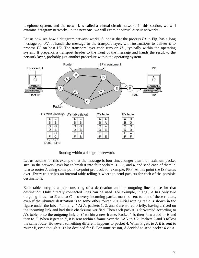
88
telephone system, and the network is called a virtual-circuit network. In this section, we will examine datagram networks; in the next one, we will examine virtual-circuit networks.
Let us now see how a datagram network works. Suppose that the process P1 in Fig. has a long
message for P2. It hands the message to the transport layer, with instructions to deliver it to
process P2 on host H2. The transport layer code runs on H1, typically within the operating
system. It prepends a transport header to the front of the message and hands the result to the
network layer, probably just another procedure within the operating system.
Routing within a datagram network.
Let us assume for this example that the message is four times longer than the maximum packet
size, so the network layer has to break it into four packets, 1, 2,3, and 4, and send each of them in
turn to router A using some point-to-point protocol, for example, PPP. At this point the ISP takes over. Every router has an internal table telling it where to send packets for each of the possible
destinations.
Each table entry is a pair consisting of a destination and the outgoing line to use for that
destination. Only directly connected lines can be used. For example, in Fig., A has only two
outgoing lines—to B and to C—so every incoming packet must be sent to one of these routers,
even if the ultimate destination is to some other router. A’s initial routing table is shown in the
figure under the label ‘‘initially.’’ At A, packets 1, 2, and 3 are stored briefly, having arrived on
the incoming link and had their checksums verified. Then each packet is forwarded according to
A’s table, onto the outgoing link to C within a new frame. Packet 1 is then forwarded to E and
then to F. When it gets to F, it is sent within a frame over the LAN to H2. Packets 2 and 3 follow
the same route. However, something different happens to packet 4. When it gets to A it is sent to
router B, even though it is also destined for F. For some reason, A decided to send packet 4 via a

89
different route than that of the first three packets. Perhaps it has learned of a traffic jam
somewhere along the ACE path and updated its routing table, as shown under the label ‘‘later.’’
The algorithm that manages the tables and makes the routing decisions is called the routing
algorithm. Routing algorithms are one of the main topics we will study in this chapter. There are
several different kinds of them, as we will see. IP (Internet Protocol), which is the basis for the
entire Internet, is the dominant example of a connectionless network service. Each packet carries
a destination IP address that routers use to individually forward each packet. The addresses are
32 bits in IPv4 packets and 128 bits in IPv6 packets.
Implementation of Connection-Oriented Service For connection-oriented service, we need a virtual-circuit network. Let us see how that works.
The idea behind virtual circuits is to avoid having to choose a new route for every packet sent, as
in. Instead, when a connection is established, a route from the source machine to the destination
machine is chosen as part of the connection setup and stored in tables inside the routers. That
route is used for all traffic flowing over the connection, exactly the same way that the telephone
system works. When the connection is released, the virtual circuit is also terminated. With
connection-oriented service, each packet carries an identifier telling which virtual circuit it
belongs to. As an example, consider the situation shown in Fig. Here, host H1 has established
connection 1 with host H2. This connection is remembered as the first entry in each of the
routing tables. The first line of A’s table says that if a packet bearing connection identifier 1
comes in from H1, it is to be sent to router C and given connection identifier 1. Similarly, the
first entry at C routes the packet to E, also with connection identifier 1.
Routing within a virtual-circuit network.
Now let us consider what happens if H3 also wants to establish a connection to H2. It chooses
connection identifier 1 (because it is initiating the connection and this is its only connection) and
tells the network to establish the virtual circuit. This leads to the second row in the tables. Note
that we have a conflict here because although A can easily distinguish connection 1 packets from
H1 from connection 1 packets from H3, C cannot do this. For this reason, A assigns a different
connection identifier to the outgoing traffic for the second connection. Avoiding conflicts of this
kind is why routers need the ability to replace connection identifiers in outgoing packets.

90
In some contexts, this process is called label switching. An example of a connection-oriented
network service is MPLS (Multi Protocol Label Switching). It is used within ISP networks in the
Internet, with IP packets wrapped in an MPLS header having a 20-bit connection identifier or
label. MPLS is often hidden from customers, with the ISP establishing long-term connections for
large amounts of traffic, but it is increasingly being used to help when quality of service is
important but also with other ISP traffic management tasks.
Comparison of Virtual-Circuit and Datagram Networks Both virtual circuits and datagrams have their supporters and their detractors. We will now attempt to summarize both sets of arguments. The major issues are listed in Fig, although purists
could probably find a counterexample for everything in the figure.
Comparison of datagram and virtual-circuit networks.
Inside the network, several trade-offs exist between virtual circuits and data grams. One trade-off
is setup time versus address parsing time. Using virtual circuits requires a setup phase, which
takes time and consumes resources. However, once this price is paid, figuring out what to do
with a data packet in a virtual-circuit network is easy: the router just uses the circuit number to
index into a table to find out where the packet goes. In a datagram network, no setup is needed
but a more complicated lookup procedure is required to locate the entry for the destination. A
related issue is that the destination addresses used in datagram networks are longer than circuit
numbers used in virtual-circuit networks because they have a global meaning. If the packets tend
to be fairly short, including a full destination address in every packet may represent a significant
amount of overhead , and hence a waste of bandwidth. Yet another issue is the amount of table
space required in router memory. A datagram network needs to have an entry for every possible
destination, whereas a virtual-circuit network just needs an entry for each virtual circuit.

91
However, this advantage is somewhat illusory since connection setup packets have to be routed
too, and they use destination addresses, the same as datagram’s do. Virtual circuits have some
advantages in guaranteeing quality of service and avoiding congestion within the network
because resources (e.g., buffers, bandwidth, and CPU cycles) can be reserved in advance, when
the connection is established. Once the packets start arriving, the necessary bandwidth and router
capacity will be there. With a datagram network, congestion avoidance is more difficult. For
transaction processing systems (e.g., stores calling up to verify credit card purchases), the
overhead required to set up and clear a virtual circuit may easily dwarf the use of the circuit. If
the majority of the traffic is expected to be of this kind, the use of virtual circuits inside the
network makes little sense. On the other hand, for long-running uses such as VPN traffic between
two corporate offices, permanent virtual circuits (that are set up manually and last for months or
years) may be useful. Virtual circuits also have a vulnerability problem. If a router crashes and
loses its memory, even if it comes back up a second later, all the virtual circuits passing through
it will have to be aborted. In contrast, if a datagram router goes down, only those users whose
packets were queued in the router at the time need suffer (and probably not even then since the
sender is likely to retransmit them shortly). The loss of a communication line is fatal to virtual
circuits using it, but can easily be compensated for if datagram’s are used. Datagram’s also allow
the routers to balance the traffic throughout the network, since routes can be changed partway
through a long sequence of packet transmissions.
PACKET SWITCHING From the discussion of routing and forwarding in the previous section, we infer that a kind of
switching occurs at the network layer. A router, in fact, is a switch that creates a connection
between an input port and an output port (or a set of output ports), just as an electrical switch
connects the input to the output to let electricity flow. Although in data communication switching
techniques are divided into two broad categories, circuit switching and packet switching, only
packet switching is used at the network layer because the unit of data at this layer is a packet.
Circuit switching is mostly used lat the physical layer; the electrical switch mentioned earlier is a
kind of circuit switch. We discussed circuit switching in Chapter 8; we discuss packet switching.
At the Network layer, a message from the upper layer is divided into manageable packets and
each packet is sent through the network. The source of the message sends the packets one by one;
the destination of the message receives the packets one by one. The destination waits for all
packets belonging to the same message to arrive before delivering the message to the upper layer.
The connecting devices in a packet-switched network still need to decide how to route the
packets to the final destination. Today, a packet-switched network can use two different
approaches to route the packets: the datagram approach and the virtual circuit approach. We
discuss both approaches in the next section.
Datagram Approach: Connectionless Service When the Internet started, to make it simple, the network layer was designed to provide a
connectionless service in which the network-layer protocol treats each packet independently,
with each packet having no relationship to any other packet. The idea was that the network layer
is only responsible for delivery of packets from the source to the destination. Id this approach,
the packets in a message mayor may not travel the same path to their destination. Figure shows
the idea. When the network layer provides a connectionless service, each packet traveling in the
Internet is an independent entity; there is no relationship between packets belonging to the same
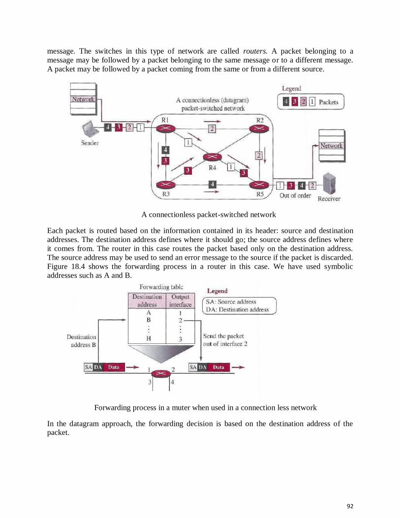
92
message. The switches in this type of network are called routers. A packet belonging to a
message may be followed by a packet belonging to the same message or to a different message.
A packet may be followed by a packet coming from the same or from a different source.
A connectionless packet-switched network
Each packet is routed based on the information contained in its header: source and destination
addresses. The destination address defines where it should go; the source address defines where
it comes from. The router in this case routes the packet based only on the destination address.
The source address may be used to send an error message to the source if the packet is discarded.
Figure 18.4 shows the forwarding process in a router in this case. We have used symbolic
addresses such as A and B.
Forwarding process in a muter when used in a connection less network
In the datagram approach, the forwarding decision is based on the destination address of the packet.

93
Virtual-Circuit Approach: Connection-Oriented Service In a connection-oriented service (also called virtual-circuit approach), there is a relationship
between all packets belonging to a message. Before all datagram’s in a message can be sent, a
virtual connection should be set up to define the path for the datagram’s. After connection setup,
the datagram’s can all follow the same path. In this type of service, not only must the packet
contain the source and destination addresses, it must also contain a flow label, a virtual circuit
identifier that defines the virtual path the packet should follow. Shortly, we will show how this
flow label is determined, but for the moment, we assume that the packet carries this label.
Although it looks as though the use of the label may make the source and destination addresses
unnecessary during the data transfer phase, parts of the Internet at the network layer still keep
these addresses. One reason is that part of the packet path may still be using the connectionless
service. Another reason is that the protocol at the network layer is designed with these addresses,
and it may take a while before they can be changed. Figure shows the concept of connection-
oriented service.
A virtual-circuit packet-switched network
Each packet is forwarded based on the label in the packet. To follow the idea of connection-
oriented design to be used in the Internet, we assume that the packet has a label when it reaches
the router. Figure 18.6 shows the idea. In this case, the forwarding decision is based on the value
of the label, or virtual circuit identifier, as it is sometimes called. To create a connection-oriented
service, a three-phase process is used: setup, data transfer, and teardown. In the setup phase, the
source and destination addresses of the sender and receiver are used to make table entries for the
connection-oriented service. In the teardown phase, the source and destination inform the router
to delete the corresponding entries. Data transfer occurs between these two phases.
Setup Phase In the setup phase, a router creates an entry for a virtual circuit. For example, suppose source .A
needs to create a virtual circuit to destination B. Two auxiliary packets need to be exchanged
between the sender and the receiver: the request packet and the acknowledgment packet.

94
Forwarding process in a router when used in a virtual-circuit
network Request packet A request packet is sent from the source to the destination. This auxiliary packet carries the source and destination addresses. Figure shows the process.
Sending request packet in a virtual-circuit network
1. Source A sends a request packet to router Rl. 2. Router Rl receives the request packet. It knows that a packet going from A to B goes 0rt
through port 3. How the router has obtained this information is a point covered later. For the

95
moment, assume that it knows the output port. The router creates an entry in its table for
this virtual circuit, but it is only able to fill three of the four columns. The router assigns the
incoming port (1) and chooses an available in rooming label (14) and the outgoing port (3).
It does not yet know the outgoing label, which will be found during the acknowledgment step. The router then forwards the packet through port 3 to router R3.
3. Router iR3 receives the setup request packet. The same events happen here as at router Rl;
three columns of the table are completed: in this case, incoming port (1)incoming label (66), and outgoing port (3).
4. Router R4 receives the setup request packet. Again, three columns are completed: incoming port (1), incoming label (22), and outgoing port (4).
5. Destination B receives the setup packet, and if it is ready to receive packets from A, it
assigns a label to the incoming packets that come from A, in this case 77, as shown in
Figure. This label lets the destination know that the packets come from A,I and not from
other sources.
Acknowledgment Packet A special Packet, called the acknowledgment packet, completes the entries in the switching tables. Figure shows the process.
Sending acknowledgments in a virtual-circuit network
1. The destination sends an acknowledgment to router R4. The acknowledgment carries the
global source and destination addresses so the router knows which entry in the table is to be
completed. The packet also carries label 77, chosen by the destination as the incoming label
for packets from A. Router R4 uses this label to complete the outgoing label column for
this entry. Note that 77 is the incoming label for destination B, but the outgoing label for
router R4. 2. Router R4 sends an acknowledgment to router R3 that contains its incoming label in the
table, chosen in the setup phase. Router R3 uses this as the outgoing label in the table. 3. Router R3 sends an acknowledgment to router Rl that contains its incoming label in the
table, chosen in the setup phase. Router RI uses this as the outgoing label in the table.

96
4. Finally router Rl sends an acknowledgment to source A that contains its incoming label
in the table, chosen in the setup phase. 5. The source uses this as the outgoing label for the data packets to be sent to destination B.
Data- Transfer Phase The second phase is called the data-transfer phase. After all routers have created their forwarding
table for a specific virtual circuit, then the network-layer packets belonging to one message can
be sent one after another. In Figure, we show the flow of a single packet, but the process is the same for 1, 2, or 100 packets. The source computer uses the label 14, which it has received from
router Rl in the setup.
Flow of one packet in an established virtual circuit
phase. Router Rl forwards the packet to router R3, but changes the label to 66.Router R3I
forwards the packet to router R4, but changes the label to 22. Finally, router R4 delivers the
packet to its final destination with the label 77. All the packets in the message follow the same
sequence of labels, and the packets arrive in order at the destination. Teardown Phase In the
teardown phase, source A, after sending all packets to B, sends a special packet called a teardown
packet. Destination B responds with a confirmation packet. All routers delete the corresponding
entries from their tables.
ROUTING ALGORITHMS The main function of the network layer is routing packets from the source machine to the destination machine. In most networks, packets will require multiple hops to make the journey.
The only notable exception is for broadcast networks, but even here routing is an issue if the
source and destination are not on the same network segment. The algorithms that choose the
routes and the data structures that they use are a major area of network layer design.
The routing algorithm is that part of the network layer software responsible for deciding which
output line an incoming packet should be transmitted on. If the network uses datagram’s
internally, this decision must be made anew for every arriving data packet since the best route
may have changed since last time. If the network uses virtual circuits internally, routing decisions
are made only when a new virtual circuit is being set up. Thereafter, data packets just follow the
already established route. The latter case is sometimes called session routing because

97
a route remains in force for an entire session (e.g., while logged in over a VPN). It is sometimes
useful to make a distinction between routing, which is making the decision which routes to use,
and forwarding, which is what happens when a packet arrives. One can think of a router as
having two processes inside it. One of them handles each packet as it arrives, looking up the
outgoing line to use for it in the routing tables. This process is forwarding. The other process is
responsible for filling in and updating the routing tables. That is where the routing algorithm
comes into play.
Regardless of whether routes are chosen independently for each packet sent or only when new
connections are established, certain properties are desirable in a routing algorithm: correctness,
simplicity, robustness, stability, fairness, and efficiency. Correctness and simplicity hardly
require comment, but the need for robustness may be less obvious at first. Once a major network
comes on the air, it may be expected to run continuously for years without system-wide failures.
During that period there will be hardware and software failures of all kinds. Hosts, routers, and
lines will fail repeatedly, and the topology will change many times. The routing algorithm should
be able to cope with changes in the topology and traffic without requiring all jobs in all hosts to
be aborted. Imagine the havoc if the network needed to be rebooted every time some router
crashed! Stability is also an important goal for the routing algorithm. There exist routing
algorithms that never converge to a fixed set of paths, no matter how long they run. A stable
algorithm reaches equilibrium and stays there. It should converge quickly too, since
communication may be disrupted until the routing algorithm has reached equilibrium. Fairness
and efficiency may sound obvious—surely no reasonable person would oppose them—but as it
turns out, they are often contradictory goals. As a simple example of this conflict, look at Fig.
Suppose that there is enough traffic between A and A′, between B and B′, and between C and C′
to saturate the horizontal links. To maximize the total flow, the X to X′ traffic should be shut off
altogether. Unfortunately, X and X′ may not see it that way. Evidently, some compromise
between global efficiency and fairness to individual connections is needed. Before we can even
attempt to find trade-offs between fairness and efficiency, we must decide what it is we seek to
optimize. Minimizing the mean packet delay is an obvious candidate to send traffic through the
network effectively, but so is maximizing total network throughput. Furthermore, these two goals
are also in conflict, since operating any queuing system near capacity implies a long queuing
delay. As a compromise, many networks attempt to minimize the distance a packet must travel,
or simply reduce the number of hops a packet must make. Either choice tends to improve the
delay and also reduce the amount of bandwidth consumed per packet, which tends to improve the
overall network throughput as well.
Routing algorithms can be grouped into two major classes: non adaptive and adaptive. Non adaptive algorithms do not base their routing decisions on any measurements or estimates of the
current topology
Network with a conflict between fairness and efficiency.
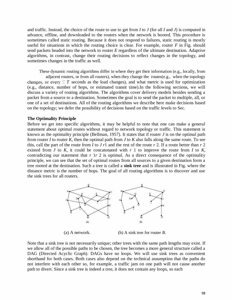
98
and traffic. Instead, the choice of the route to use to get from I to J (for all I and J) is computed in
advance, offline, and downloaded to the routers when the network is booted. This procedure is
sometimes called static routing. Because it does not respond to failures, static routing is mostly
useful for situations in which the routing choice is clear. For example, router F in Fig. should
send packets headed into the network to router E regardless of the ultimate destination. Adaptive
algorithms, in contrast, change their routing decisions to reflect changes in the topology, and
sometimes changes in the traffic as well.
These dynamic routing algorithms differ in where they get their information (e.g., locally, from
adjacent routers, or from all routers), when they change the routes(e.g., when the topology T seconds as the load changes), and what metric is used for optimization
(e.g., distance, number of hops, or estimated transit time).In the following sections, we will
discuss a variety of routing algorithms. The algorithms cover delivery models besides sending a
packet from a source to a destination. Sometimes the goal is to send the packet to multiple, all, or
one of a set of destinations. All of the routing algorithms we describe here make decisions based
on the topology; we defer the possibility of decisions based on the traffic levels to Sec.
The Optimality Principle Before we get into specific algorithms, it may be helpful to note that one can make a general
statement about optimal routes without regard to network topology or traffic. This statement is
known as the optimality principle (Bellman, 1957). It states that if router J is on the optimal path
from router I to router K, then the optimal path from J to K also falls along the same route. To see
this, call the part of the route from I to J r1 and the rest of the route r 2. If a route better than r 2
existed from J to K, it could be concatenated with r 1 to improve the route from I to K,
contradicting our statement that r 1r 2 is optimal. As a direct consequence of the optimality
principle, we can see that the set of optimal routes from all sources to a given destination form a
tree rooted at the destination. Such a tree is called a sink tree and is illustrated in Fig. where the
distance metric is the number of hops. The goal of all routing algorithms is to discover and use
the sink trees for all routers.
(a) A network. (b) A sink tree for router B.
Note that a sink tree is not necessarily unique; other trees with the same path lengths may exist. If
we allow all of the possible paths to be chosen, the tree becomes a more general structure called a
DAG (Directed Acyclic Graph). DAGs have no loops. We will use sink trees as convenient
shorthand for both cases. Both cases also depend on the technical assumption that the paths do
not interfere with each other so, for example, a traffic jam on one path will not cause another
path to divert. Since a sink tree is indeed a tree, it does not contain any loops, so each
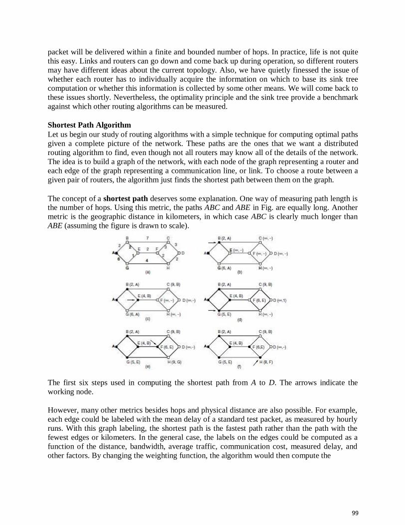
99
packet will be delivered within a finite and bounded number of hops. In practice, life is not quite
this easy. Links and routers can go down and come back up during operation, so different routers
may have different ideas about the current topology. Also, we have quietly finessed the issue of
whether each router has to individually acquire the information on which to base its sink tree
computation or whether this information is collected by some other means. We will come back to
these issues shortly. Nevertheless, the optimality principle and the sink tree provide a benchmark
against which other routing algorithms can be measured.
Shortest Path Algorithm Let us begin our study of routing algorithms with a simple technique for computing optimal paths
given a complete picture of the network. These paths are the ones that we want a distributed
routing algorithm to find, even though not all routers may know all of the details of the network.
The idea is to build a graph of the network, with each node of the graph representing a router and
each edge of the graph representing a communication line, or link. To choose a route between a
given pair of routers, the algorithm just finds the shortest path between them on the graph.
The concept of a shortest path deserves some explanation. One way of measuring path length is the number of hops. Using this metric, the paths ABC and ABE in Fig. are equally long. Another
metric is the geographic distance in kilometers, in which case ABC is clearly much longer than
ABE (assuming the figure is drawn to scale).
The first six steps used in computing the shortest path from A to D. The arrows indicate the
working node.
However, many other metrics besides hops and physical distance are also possible. For example,
each edge could be labeled with the mean delay of a standard test packet, as measured by hourly
runs. With this graph labeling, the shortest path is the fastest path rather than the path with the
fewest edges or kilometers. In the general case, the labels on the edges could be computed as a
function of the distance, bandwidth, average traffic, communication cost, measured delay, and
other factors. By changing the weighting function, the algorithm would then compute the

100
‘‘shortest’’ path measured according to any one of a number of criteria or to a combination of
criteria. Several algorithms for computing the shortest path between two nodes of a graph are
known. This one is due to Dijkstra (1959) and finds the shortest paths between a source and all
destinations in the network. Each node is labeled (in parentheses) with its distance from the
source node along the best known path. The distances must be non-negative, as they will be if
they are based on real quantities like bandwidth and delay. Initially, no paths are known, so all
nodes are labeled with infinity. As the algorithm proceeds and paths are found, the labels may
change, reflecting better paths. A label may be either tentative or permanent. Initially, all labels
are tentative. When it is discovered that a label represents the shortest possible path from the
source to that node, it is made permanent and never changed thereafter. To illustrate how the
labeling algorithm works, look at the weighted, undirected graph of Fig., where the weights
represent, for example, distance. We want to find the shortest path from A to D. We start out by
marking node A as permanent, indicated by a filled-in circle. Then we examine, in turn, each of
the nodes adjacent to A (the working node), relabeling each one with the distance to A. Whenever
a node is relabeled, we also label it with the node from which the probe was made so that we can
reconstruct the final path later. If the network had more than one shortest path from A to D and
we wanted to find all of them, we would need to remember all of the probe nodes that could
reach a node with the same distance. Having examined each of the nodes adjacent to A, we
examine all the tentatively labeled nodes in the whole graph and make the one with the smallest
label permanent, as shown in Fig. (b). this one becomes the new working node. We now start at
B and examine all nodes adjacent to it. If the sum of the label on B and the distance from B to the
node being considered is less than the label on that node, we have a shorter path, so the node is
relabeled. After all the nodes adjacent to the working node have been inspected and the tentative
labels changed if possible, the entire graph is searched for the tentatively labeled node with the
smallest value. This node is made permanent and becomes the working node for the next round.
Figure shows the first six steps of the algorithm. To see why the algorithm works, look at Fig. (c). At this point we have just made E permanent. Suppose that there were a shorter path than
ABE, say AXYZE (for some X and Y). There are two possibilities: either node Z has already been
made permanent, or it has not been. If it has, then E has already been probed (on the round
following the one when Z was made permanent), so the AXYZE path has not escaped our
attention and thus cannot be a shorter path. Now consider the case where Z is still tentatively
labeled. If the label at Z is greater than or equal to that at E, then AXYZE cannot be a shorter path
than ABE. If the label is less than that of E, then Z and not E will become permanent first,
allowing E to be probed from Z. This algorithm is given in Fig. The global variables n and dist
describe the graph and are initialized before shortest path is called. The only difference between
the program and the algorithm described above is that in Fig., we compute the shortest path
starting at the terminal node, t, rather than at the source node, s. Since the shortest paths from t to
s in an undirected graph are the same as the shortest paths from s to t, it does not matter at which
end we begin. The reason for searching backward is that each node is labeled with its predecessor
rather than its successor. When the final path is copied into the output variable, path, the path is
thus reversed. The two reversal effects cancel, and the answer is produced in the correct order.
Flooding
When a routing algorithm is implemented, each router must make decisions based on local knowledge, not the complete picture of the network. A simple local technique is flooding, in

101
which every incoming packet is sent out on every outgoing line except the one it arrived on.
Flooding obviously generates vast numbers of duplicate packets, in fact, an infinite number
unless some measures are taken to damp the process. One such measure is to have a hop counter
contained in the header of each packet that is decremented at each hop, with the packet being
discarded when the counter reaches zero. Ideally, the hop counter should be initialized to the
length of the path from source to destination. If the sender does not know how long the path is, it
can initialize the counter to the worst case, namely, the full diameter of the network.
Flooding with a hop count can produce an exponential number of duplicate packets as the hop
count grows and routers duplicate packets they have seen before. A better technique for
damming the flood is to have routers keep track of which packets have been flooded, to avoid
sending them out a second time. One way to achieve this goal is to have the source router put a
sequence number in each packet it receives from its hosts. Each router then needs a list per
source router telling which sequence numbers originating at that source have already been seen.
If an incoming packet is on the list, it is not flooded.
To prevent the list from growing without bound, each list should be augmented by a counter, k,
meaning that all sequence numbers through k have been seen. When a packet comes in, it is easy
to check if the packet has already been flooded (by comparing its sequence number to k; if so, it
is discarded. Furthermore, the full list below k is not needed, since k effectively summarizes it.
Flooding is not practical for sending most packets, but it does have some important uses. First, it
ensures that a packet is delivered to every node in the network. This may be wasteful if there is a
single destination that needs the packet, but it is effective for broadcasting information. In
wireless networks, all messages transmitted by a station can be received by all other stations
within its radio range, which is, in fact, flooding, and some algorithms utilize this property.
Second, flooding is tremendously robust. Even if large numbers of routers are blown to bits (e.g.,
in a military network located in a war zone), flooding will find a path if one exists, to get a
packet to its destination. Flooding also requires little in the way of setup. The routers only need
to know their neighbors. This means that flooding can be used as a building block for other
routing algorithms that are more efficient but need more in the way of setup. Flooding can also be used as a metric against which other routing algorithms can be compared. Flooding always chooses the shortest path
because it chooses every possible path in parallel. Consequently, no other algorithm can produce
a shorter delay (if we ignore the overhead generated by the flooding process itself).
Distance Vector Routing Computer networks generally use dynamic routing algorithms that are more complex than
flooding, but more efficient because they find shortest paths for the current topology. Two
dynamic algorithms in particular, distance vector routing and link state routing, are the most
popular. In this section, we will look at the former algorithm. In the following section, we will
study the latter algorithm. A distance vector routing algorithm operates by having each router
maintain a table (i.e., a vector) giving the best known distance to each destination and which link
to use to get there. These tables are updated by exchanging information with the neighbors.
Eventually, every router knows the best link to reach each destination. The distance vector
routing algorithm is sometimes called by other names, most commonly the distributed Bellman-
Ford routing algorithm, after the researchers who developed it (Bellman, 1957; and Ford and
Fulkerson, 1962). It was the original ARPANET routing algorithm and was also used in the

102
Internet under the name RIP. In distance vector routing, each router maintains a routing table
indexed by, and containing one entry for each router in the network. This entry has two parts: the
preferred outgoing line to use for that destination and an estimate of the distance to that
destination. The distance might be measured as the number of hops or using another metric, as
we discussed for computing shortest paths. The router is assumed to know the ‘‘distance’’ to
each of its neighbors. If the metric is hops, the distance is just one hop. If the metric is
propagation delay, the router can measure it directly with special ECHO packets that the receiver
just timestamps and sends back as fast as it can. As an example, assume that delay is used as a
metric and that the router knows the delay to each of its neighbors. Once every T m sec, each
router sends to each neighbor a list of its estimated delays to each destination. It also receives a
similar list from each neighbor. Imagine that one of these tables has just come in from neighbor
X, with Xi being X’s estimate of how long it takes to get to router i. If the router knows that the delay to X is m m sec, it also knows that it can reach router i via X in Xi m msec. By performing
this calculation for each neighbor, a router can find out which estimate seems the best and use that estimate and the corresponding link in its new routing table. Note that the old routing table is
not used in the calculation. This updating process is illustrated in Fig. 5-9. Part (a) shows a network. The first four columns of part (b) show the delay vectors received from the
neighbors of router J. A claims to have a 12-msec delay to B, a 25-msec delay to C, a 40-msec
delay to D, etc. Suppose that J has measured or estimated its delay to its neighbors, A, I, H, and K, as 8, 10, 12, and 6 m sec, respectively.
(a) A network. (b) Input from A, I, H, K, and the new routing table for J.
Consider how J computes its new route to router G. It knows that it can get to A in 8 m sec, and
furthermore A claims to be able to get to G in 18 m sec, so J knows it can count on a delay of 26
m sec to G if it forwards packets bound for G to A. Similarly, it computes the delay to G via I, H,
and K as 41 (31 + 10), 18 (6 + 12), and 37 (31 + 6) m sec, respectively. The best of these values
is 18, so it makes an entry in its routing table that the delay to G is 18 m sec and that the route to
use is via H. The same calculation is performed for all the other destinations, with the new
routing table shown in the last column of the figure.
The Count-to-Infinity Problem The settling of routes to best paths across the network is called convergence. Distance vector
routing is useful as a simple technique by which routers can collectively compute shortest paths,

103
but it has a serious drawback in practice: although it converges to the correct answer, it may do
so slowly. In particular, it reacts rapidly to good news, but leisurely to bad news. Consider a
router whose best route to destination X is long. If, on the next exchange, neighbor A suddenly
reports a short delay to X, the router just switches over to using the line to A to send traffic to X.
In one vector exchange, the good news is processed. To see how fast good news propagates,
consider the five-node (linear) network of Fig. 5-10, where the delay metric is the number of
hops. Suppose A is down initially and all the other routers know this. In other words, they have
all recorded the delay to A as infinity.
The count-to-infinity problem.
When A comes up, the other routers learn about it via the vector exchanges. For simplicity, we
will assume that there is a gigantic going somewhere that is struck periodically to initiate a vector
exchange at all routers simultaneously. At the time of the first exchange, B learns that its left-
hand neighbor has zero delay to A. B now makes an entry in its routing table indicating that A is
one hop away to the left. All the other routers still think that A is down. At this point, the routing
table entries for A are as shown in the second row of Fig. (a). On the next exchange, C learns that
B has a path of length 1 to A, so it updates its routing table to indicate a path of length 2, but D
and E do not hear the good news until later. Clearly, the good news is spreading at the rate of one
hop per exchange. In a network whose longest path is of length N hops, within N exchanges
everyone will know about newly revived links and routers. Now let us consider the situation of
(b), in which all the links and routers are initially up. Routers B, C, D, and E have distances to A
of 1, 2, 3, and 4 hops, respectively. Suddenly, either A goes down or the link between A and B is
cut (which is effectively the same thing from B’s point of view).At the first packet exchange, B
does not hear anything from A. Fortunately, C says ‘‘Do not worry; I have a path to A of length
2.’’ Little does B suspect that C’s path runs through B itself . For all B knows, C might have ten
links all with separate paths to A of length 2. As a result, B thinks it can reach A via C, with a
path length of 3. D and E do not update their entries for A on the first exchange.
On the second exchange, C notices that each of its neighbors claims to have a path to A of length 3. It picks one of them at random and makes its new distance to A 4, as shown in the third row of
Fig. 5-10(b). Subsequent exchanges produce the history shown in the rest of Fig. 5-10(b).From
this figure, it should be clear why bad news travels Slowly: no router ever has a value more than
one higher than the minimum of all its neighbors. Gradually, all routers work their way up to
infinity, but the number of exchanges required depends on the numerical value used for infinity.
For this reason, it is wise to set infinity to the longest path plus 1.Not entirely surprisingly, this
problem is known as the count-to-infinity problem. There have been many attempts to solve it,
for example, preventing routers from advertising their best paths back to the neighbors from

104
which they heard them with the split horizon with poisoned reverse rule discussed in RFC
1058.However, none of these heuristics work well in practice despite the colorful names. The
core of the problem is that when X tells Y that it has a path somewhere, Y has no way of knowing
whether it itself is on the path.
Hierarchical Routing As networks grow in size, the router routing tables grow proportionally. Not only is router
memory consumed by ever-increasing tables, but more CPU time is needed to scan them and
more bandwidth is needed to send status reports about them. At a certain point, the network may
grow to the point where it is no longer feasible for every router to have an entry for every other
router, so the routing will have to be done hierarchically, as it is in the telephone network. When
hierarchical routing is used, the routers are divided into what we will call regions. Each router
knows all the details about how to route packets to destinations within its own region but knows
nothing about the internal structure of other regions. When different networks are interconnected,
it is natural to regard each one as a separate region to free the routers in one network from having
to know the topological structure of the other ones. For huge networks, a two-level hierarchy
may be insufficient; it may be necessary to group the regions into clusters, the clusters into
zones, the zones into groups, and so on, until we run out of names for aggregations. As an
example of a multilevel hierarchy, consider how a packet might be routed from Berkeley,
California, to Malindi, Kenya. The Berkeley router would know the detailed topology within
California but would send all out-of-state traffic to the Los Angeles router. The Los Angeles
router would be able to route traffic directly to other domestic routers but would send all foreign
traffic to New York. The New York router would be programmed to direct all traffic to the router
in the destination country responsible for handling foreign traffic, say, in Nairobi. Finally, the
packet would work its way down the tree in Kenya until it got to Malindi. Figure gives a
quantitative example of routing in a two-level hierarchy with five regions. The full routing table
for router 1A has 17 entries, as shown in Fig. (b). When routing is done hierarchically, as in Fig.
5-14(c), there are entries for all the local routers, as before, but all other regions are condensed
into a single router, so all traffic for region 2 goes via the 1B-2A line, but the rest of the remote
traffic goes via the 1C-3B line. Hierarchical routing has reduced the table from 17 to 7 entries. As
the ratio of the number of regions to the number of routers per region grows, the savings in table
space increase. Unfortunately, these gains in space are not free. There is a penalty to be paid:
increased path length. For example, the best route from 1A to 5C is via region 2,but with
hierarchical routing all traffic to region 5 goes via region 3, because that is better for most
destinations in region 5.When a single network becomes very large, an interesting question is
‘‘how many levels should the hierarchy have?’’ For example, consider a network with 720
routers. If there is no hierarchy, each router needs 720 routing table entries. If the network is
partitioned into 24 regions of 30 routers each, each router needs 30 local entries plus 23 remote
entries for a total of 53 entries. If a three-level hierarchy is chosen, with 8 clusters each
containing 9 regions of 10 routers, each router needs 10 entries for local routers, 8 entries for
routing to other regions within its own cluster, and 7 entries for distant clusters, for a total of 25
entries. Kamoun and Kleinrock (1979) discovered that the optimal number of levels for an N
router network is ln N, requiring a total of e ln N entries per router. They have also shown that
the increase in effective mean path length caused by hierarchical routing is sufficiently small that
it is usually acceptable.

105
Hierarchical routing.
CONGESTION CONTROL ALGORITHMS
Too many packets present in (a part of) the network causes packet delay and loss that degrades
performance. This situation is called congestion. The network and transport layers share the
responsibility for handling congestion. Since congestion occurs within the network, it is the
network layer that directly experiences it and must ultimately determine what to do with the
excess packets. However, the most effective way to control congestion is to reduce the load that
the transport layer is placing on the network. This requires the network and transport layers to
work together. In this chapter we will look at the network aspects of congestion. In Chap. 6, we
will complete the topic by covering the transport aspects of congestion. Figure depicts the onset
of congestion. When the number of packets hosts send into the network is well within its
carrying capacity, the number delivered is proportional to the number sent. If twice as many are
sent, twice as many are delivered. However, as the offered load approaches the carrying capacity,
bursts of traffic occasionally fill up the buffers inside routers and some packets are lost. These
lost packets consume some of the capacity, so the number of delivered packets falls below the
ideal curve. The network is now congested.
With too much traffic, performance drops sharply.
Unless the network is well designed, it may experience a congestion collapse, in which performance plummets as the offered load increases beyond the capacity. This can happen

106
because packets can be sufficiently delayed inside the network that they are no longer useful
when they leave the network. For example, in the early Internet, the time a packet spent waiting
for a backlog of packets ahead of it to be sent over a slow 56-kbps link could reach the maximum
time it was allowed to remain in the network. It then had to be thrown away. A different failure
mode occurs when senders retransmit packets that are greatly delayed, thinking that they have
been lost. In this case, copies of the same packet will be delivered by the network, again wasting
its capacity. To capture these factors, the y-axis of Fig. is given as good put, which is the rate at
which useful packets are delivered by the network. We would like to design networks that avoid
congestion where possible and do not suffer from congestion collapse if they do become
congested. Unfortunately, congestion cannot wholly be avoided. If all of a sudden, streams of
packets begin arriving on three or four input lines and all need the same output line, a queue will
build up. If there is insufficient memory to hold all of them, packets will be lost. Adding more
memory may help up to a point, but Nagle (1987) realized that if routers have an infinite amount
of memory, congestion gets worse, not better. This is because by the time packets get to the front
of the queue, they have already timed out (repeatedly) and duplicates have been sent. This makes
matters worse, not better—it leads to congestion collapse. Low-bandwidth links or routers that
process packets more slowly than the line rate can also become congested. In this case, the
situation can be improved by directing some of the traffic away from the bottleneck to other parts
of the network. Eventually, however, all regions of the network will be congested. In this
situation, there is no alternative but to shed load or build a faster network. It is worth pointing out
the difference between congestion control and flow control, as the relationship is a very subtle
one. Congestion control has to do with making sure the network is able to carry the offered
traffic. It is a global issue, involving the behavior of all the hosts and routers. Flow control, in
contrast, relates to the traffic between a particular sender and a particular receiver. Its job is to
make sure that a fast sender cannot continually transmit data faster than the receiver is able to
absorb it. To see the difference between these two concepts, consider a network made up of 100-
Gbps fiber optic links on which a supercomputer is trying to force feed a large file to a personal
computer that is capable of handling only 1 Gbps. Although there is no congestion (the network
itself is not in trouble), flow control is needed to force the supercomputer to stop frequently to
give the personal computer chance to breathe. At the other extreme, consider a network with 1-
Mbps lines and 1000 large computers, half of which are trying to transfer files at 100 kbps to the
other half. Here, the problem is not that of fast senders overpowering slow receivers, but that the
total offered traffic exceeds what the network can handle.
The reason congestion control and flow control are often confused is that the best way to handle
both problems is to get the host to slow down. Thus, a host can get a ‘‘slow down’’ message
either because the receiver cannot handle the load or because the network cannot handle it. We
will come back to this point in Chap. 6. We will start our study of congestion control by looking
at the approaches that can be used at different time scales. Then we will look at approaches to
preventing congestion from occurring in the first place, followed by approaches for coping with
it once it has set in.
Approaches to Congestion Control The presence of congestion means that the load is (temporarily) greater than the resources (in a
part of the network) can handle. Two solutions come to mind: increase the resources or decrease

107
the load. As shown in Fig., these solutions are usually applied on different time scales to either prevent congestion or react to it once it has occurred.
Timescales of approaches to congestion control.
The most basic way to avoid congestion is to build a network that is well matched to the traffic
that it carries. If there is a low-bandwidth link on the path along which most traffic is directed,
congestion is likely. Sometimes resources on spare routers or enabling lines that are normally
used only as backups (to make the system fault tolerant) or purchasing bandwidth on the open
market. More often, links and routers that are regularly heavily utilized are upgraded at the
earliest opportunity. This is called provisioning and happens on a time scale of months, driven
by long-term traffic trends. To make the most of the existing network capacity, routes can be
tailored to traffic patterns that change during the day as network user’s wake and sleep in
different time zones. For example, routes may be changed to shift traffic away from heavily used
paths by changing the shortest path weights. Some local radio stations have helicopters flying
around their cities to report on road congestion to make it possible for their mobile listeners to
route their packets (cars) around hotspots. This is called traffic-aware routing. Splitting traffic
across multiple paths is also helpful. However, sometimes it is not possible to increase capacity.
The only way then to beat back the congestion is to decrease the load. In a virtual-circuit
network, new connections can be refused if they would cause the network to become congested.
This is called admission control. At a finer granularity, when congestion is imminent the
network can deliver feedback to the sources whose traffic flows are responsible for the problem.
The network can request these sources to throttle their traffic, or it can slow down the traffic
itself. Two difficulties with this approach are how to identify the onset of congestion, and how to
inform the source that needs to slow down. To tackle the first issue, routers can monitor the
average load, queuing delay, or packet loss. In all cases, rising numbers indicate growing
congestion. To tackle the second issue, routers must participate in a feedback loop with the
sources. For a scheme to work correctly, the time scale must be adjusted carefully. If every time
two packets arrive in a row, a router yells STOP and every time a router is idle for 20 sec, it yells
GO, the system will oscillate wildly and never converge. On the other hand, if it waits 30
minutes to make sure before saying anything, the congestion-control mechanism will react too
sluggishly to be of any use. Delivering timely feedback is a nontrivial matter. An added concern
is having routers send more messages when the network is already congested.
Finally, when all else fails, the network is forced to discard packets that it cannot deliver. The
general name for this is load shedding. A good policy for choosing which packets to discard can help to prevent congestion collapse.
Traffic-Aware Routing The first approach we will examine is traffic-aware routing. The routing schemes we looked at in
Sec used fixed link weights. These schemes adapted to changes in topology, but not to changes
in load. The goal in taking load into account when computing routes is to shift traffic away from

108
hotspots that will be the first places in the network to experience congestion. The most direct way
to do this is to set the link weight to be a function of the (fixed) link bandwidth and propagation
delay plus the (variable) measured load or average queuing delay. Least-weight paths will then
favor paths that are more lightly loaded, all else being equal. Traffic-aware routing was used in
the early Internet according to this model (Khanna and Zinky, 1989). However, there is a peril.
Consider the network of Fig., which is divided into two parts, East and West, connected by two
links, CF and EI. Suppose that most of the traffic between East and West is using link CF, and,
as a result, this link is heavily loaded with long delays. Including queuing delay in the weight
used for the shortest path calculation will make EI more attractive. After the new routing tables
have been installed, most of the East-West traffic will now go over EI, loading this link.
Consequently, in the next update, CF will appear to be the shortest path. As a result, the routing
tables may oscillate wildly, leading to erratic routing and many potential problems.
A network in which the East and West parts are connected by two links.
If load is ignored and only bandwidth and propagation delay are considered, this problem does
not occur. Attempts to include load but change weights within a narrow range only slow down
routing oscillations. Two techniques can contribute to a successful solution. The first is multipath
routing, in which there can be multiple paths from a source to a destination. In our example this
means that the traffic can be spread across both of the East to West links. The second one is for
the routing scheme to shift traffic across routes slowly enough that it is able to converge, as in the
scheme of Gallagher (1977).Given these difficulties, in the Internet routing protocols do not
generally adjust their routes depending on the load. Instead, adjustments are made outside the
routing protocol by slowly changing its inputs. This is called traffic engineering.
Admission Control One technique that is widely used in virtual-circuit networks to keep congestion at bay is
admission control. The idea is simple: do not set up a new virtual circuit unless the network can
carry the added traffic without becoming congested. Thus, attempts to set up a virtual circuit may
fail. This is better than the alternative, as letting more people in when the network is busy just
makes matters worse. By analogy, in the telephone system, when a switch gets overloaded it
practices admission control by not giving dial tones. The trick with this approach is working out
when a new virtual circuit will lead to congestion. The task is straightforward in the telephone
network because of the fixed bandwidth of calls (64 kbps for uncompressed audio). However,
virtual circuits in computer networks come in all shapes and sizes. Thus, the circuit must come
with some characterization of its traffic if we are to apply admission control. Traffic is often
described in terms of its rate and shape. The problem of how to describe it in a simple yet

109
meaningful way is difficult because traffic is typically bursty—the average rate is only half the
story. For example, traffic that varies while browsing the Web is more difficult to handle than a
streaming movie with the same long-term throughput because the bursts of Web traffic are more
likely to congest routers in the network. A commonly used descriptor that captures this effect is
the leaky bucket or token bucket. A leaky bucket has two parameters that bound the average
rate and the instantaneous burst size of traffic. Since leaky buckets are widely used for quality of
service, we will go over them in detail in Sec. Armed with traffic descriptions, the network can
decide whether to admit the new virtual circuit. One possibility is for the network to reserve
enough capacity along the paths of each of its virtual circuits that congestion will not occur. In
this case, the traffic description is a service agreement for what the network will guarantee its
users. We have prevented congestion but veered into the related topic of quality of service a little
too early; we will return to it in the next section. Even without making guarantees, the network
can use traffic descriptions for admission control. The task is then to estimate how many circuits
will fit within the carrying capacity of the network without congestion. Suppose that virtual
circuits that may blast traffic at rates up to 10 Mbps all pass through the same 100-Mbps physical
link. How many circuits should be admitted? Clearly, 10 circuits can be admitted without risking
congestion, but this is wasteful in the normal case since it may rarely happen that all 10 are
transmitting full blast at the same time. In real networks, measurements of past behavior that
capture the statistics of transmissions can be used to estimate the number of circuits to admit, to
trade better performance for acceptable risk. Admission control can also be combined with
traffic-aware routing by considering routes around traffic hotspots as part of the setup procedure.
For example, consider the network illustrated in Fig (a), in which two routers are congested, as
indicated.
(a) A congested network. (b) The portion of the network that is not congested. A virtual circuit from A to B is also shown.
Suppose that a host attached to router A wants to set up a connection to a host attached to router B. Normally, this connection would pass through one of the congested routers. To avoid this
situation, we can redraw the network as shown in Fig. 5-24(b), omitting the congested routers
and all of their lines. The dashed line shows a possible route for the virtual circuit that avoids the
congested routers. Shaikh et al. (1999) give a design for this kind of load-sensitive routing.

110
UNIT – IV
Internetworking
Until now, we have implicitly assumed that there is a single homogeneous network, with each
machine using the same protocol in each layer. Unfortunately, this assumption is wildly
optimistic. Many different networks exist, including PANs, LANs, MANs, and WANs. We have
described Ethernet, Internet over cable, the fixed and mobile telephone networks, 802.11, 802.16,
and more. Numerous protocols are in widespread use across these networks in every layer. In the
following sections, we will take a careful look at the issues that arise when two or more networks
are connected to form an internetwork, or more simply an internet.
It would be much simpler to join networks together if everyone used a single networking
technology, and it is often the case that there is a dominant kind of network, such as Ethernet.
Some pundits speculate that the multiplicity of technologies will go away as soon as everyone
realizes how wonderful [fill in your favorite network] is. Do not count on it. History shows this
to be wishful thinking. Different kinds of networks grapple with different problems, so, for
example, Ethernet and satellite networks are always likely to differ. Reusing existing systems,
such as running data networks on top of cable, the telephone network, and power lines, adds
constraints that cause the features of the networks to diverge. Heterogeneity is here to stay. If
there will always be different networks, it would be simpler if we did not need to interconnect
them. This also is unlikely. Bob Metcalfe postulated that the value of a network with N nodes is
the number of connections that may be made between the nodes, or N2 (Gilder, 1993). This means that large networks are much more valuable than small networks because they allow
many more connections, so there always will be an incentive to combine smaller networks. The
Internet is the prime example of this interconnection. (We will write Internet with a capital ‘‘I’’
to distinguish it from other internets, or connected networks.)The purpose of joining all these
networks is to allow users on any of them to communicate with users on all the other ones. When
you pay an ISP for Internet service, you may be charged depending on the bandwidth of your
line, but what you are really paying for is the ability to exchange packets with any other host that
is also connected to the Internet. After all, the Internet would not be very popular if you could
only send packets to other hosts in the same city. Since networks often differ in important ways,
getting packets from one network to another is not always so easy. We must address problems of
heterogeneity, and also problems of scale as the resulting internet grows very large. We will
begin by looking at how networks can differ to see what we are up against. Then we shall see the
approach used so successfully by IP (Internet Protocol), the network layer protocol of the
Internet, including techniques for tunneling through networks, routing in internetworks, and
packet fragmentation.
Tunneling Handling the general case of making two different networks interwork is exceedingly difficult.
However, there is a common special case that is manageable even for different network
protocols. This case is where the source and destination hosts are on the same type of network,
but there is a different network in between. As an example, think of an international bank with
an IPv6 network in Paris, an IPv6 network in London and connectivity between the offices via
the IPv4 Internet. This situation is shown in Fig.

111
Tunneling a packet from Paris to London.
The solution to this problem is a technique called tunneling. To send an IP packet to a host in the London office, a host in the Paris office constructs the packet containing an IPv6 address in
London, and sends it to the multiprotocol router that connects the Paris IPv6 network to the IPv4
Internet. When this router gets the IPv6 packet, it encapsulates the packet with an IPv4 header
addressed to the IPv4 side of the multiprotocol router that connects to the London IPv6 network.
That is, the router puts a (IPv6) packet inside a (IPv4) packet. When this wrapped packet arrives, the London router removes the original IPv6 packet and sends it onward to the destination host.
The path through the IPv4 Internet can be seen as a big tunnel extending from one multiprotocol
router to the other. The IPv6 packet just travels from one end of the tunnel to the other, snug in its nice box. It does not have to worry about dealing with IPv4 at all. Neither do the hosts in Paris
or London. Only the multiprotocol routers have to understand both IPv4 and IPv6 packets. In
effect, the entire trip from one multiprotocol router to the other is like a hop over a single link.
An analogy may make tunneling clearer. Consider a person driving her car from Paris to London.
Within France, the car moves under its own power, but when it hits the English Channel, it is
loaded onto a high-speed train and transported to England through the Chunnel (cars are not
permitted to drive through the Chunnel). Effectively, the car is being carried as freight, as
depicted in Fig. At the far end, the car is let loose on the English roads and once again continues
to move under its own power. Tunneling of packets through a foreign network works the same
way. Tunneling is widely used to connect isolated hosts and networks using other networks. The
network that results is called an overlay since it has effectively been overlaid on the base
network. Deployment of a network protocol with a new feature is a common reason, as our
‘‘IPv6 over IPv4’’ example shows. The disadvantage of tunneling is that none of the hosts on the
network that are tunneled over can be reached because the packets cannot escape in the middle of
the tunnel.
Tunneling a car from France to England.
112
However, this limitation of tunnels is turned into an advantage with VPNs (Virtual Private Networks). A VPN is simply an overlay that is used to provide a measure of security.
Internetwork Routing Routing through an internet poses the same basic problem as routing within a single network, but
with some added complications. To start, the networks may internally use different routing
algorithms. For example, one network may use link state routing and another distance vector
routing. Since link state algorithms need to know the topology but distance vector algorithms do
not, this difference alone would make it unclear how to find the shortest paths across the internet.
Networks run by different operators lead to bigger problems. First, the operators may have
different ideas about what is a good path through the network. One operator may want the route
with the least delay, while another may want the most inexpensive route. This will lead the
operators to use different quantities to set the shortest-path costs (e.g., milliseconds of delay vs.
monetary cost). The weights will not be comparable across networks, so shortest paths on the
internet will not be well defined. Worse yet, one operator may not want another operator to even
know the details of the paths in its network, perhaps because the weights and paths may reflect
sensitive information (such as the monetary cost) that represents a competitive business
advantage. Finally, the internet may be much larger than any of the networks that comprise it. It
may therefore require routing algorithms that scale well by using a hierarchy; even if none of the
individual networks need to use a hierarchy. All of these considerations lead to a two-level
routing algorithm. Within each network, an intra domain or interior gateway protocol is used
for routing.(‘‘Gateway’’ is an older term for ‘‘router.’’) It might be a link state protocol of the
kind we have already described. Across the networks that make up the internet, an inter domain
or exterior gateway protocol is used. The networks may all use different intra domain protocols,
but they must use the same inter domain protocol. In the Internet, the inter domain routing
protocol is called BGP (Border Gateway Protocol).
We will there is one more important term to introduce. Since each network is operated
independently of all the others, it is often referred to as an AS (Autonomous System). A good
mental model for an AS is an ISP network. In fact, an ISP network may be comprised of more
than one AS, if it is managed, or, has been acquired, as multiple networks. But the difference is
usually not significant. The two levels are usually not strictly hierarchical, as highly suboptimal
paths might result if a large international network and a small regional network were both
abstracted to be a single network. However, relatively little information about routes within the
networks is exposed to find routes across the internetwork. This helps to address all of the complications. It improves scaling and lets operators freely select
routes within their own networks using a protocol of their choosing. It also does not require
weights to be compared across networks or expose sensitive information outside of networks.
However, we have said little so far about how the routes across the networks of the internet are
determined. In the Internet, a large determining factor is the business arrangements between
ISPs. Each ISP may charge or receive money from the other ISPs for carrying traffic. Another
factor is that if internetwork routing requires crossing international boundaries, various laws may
suddenly come into play, such as Sweden’s strict privacy laws about exporting personal data
about Swedish citizens from Sweden. All of these nontechnical factors are wrapped up in the

113
concept of a routing policy that governs the way autonomous networks select the routes that they use. We will return to routing policies when we describe BGP.
Packet Fragmentation Each network or link imposes some maximum size on its packets. These limits have various causes, among them 1. Hardware (e.g., the size of an Ethernet frame).
2. Operating system (e.g., all buffers are 512 bytes). 3. Protocols (e.g., the number of bits in the packet length field).
4. Compliance with some (inter)national standard.
5. Desire to reduce error-induced retransmissions to some level.
6. Desire to prevent one packet from occupying the channel too long.
The result of all these factors is that the network designers are not free to choose any old
maximum packet size they wish. Maximum payloads for some common technologies are 1500
bytes for Ethernet and 2272 bytes for 802.11. IP is more generous, allows for packets as big as
65,515 bytes. Hosts usually prefer to transmit large packets because this reduces packet
overheads such as bandwidth wasted on header bytes. An obvious internetworking problem
appears when a large packet wants to travel through a network whose maximum packet size is
too small. This nuisance has been a persistent issue, and solutions to it have evolved along with
much experience gained on the Internet. One solution is to make sure the problem does not occur
in the first place. However, this is easier said than done. A source does not usually know the path
a packet will take through the network to a destination, so it certainly does not know how small
packets must be to get there. This packet size is called the Path MTU (Path Maximum
Transmission Unit). Even if the source did know the path MTU, packets are routed
independently in a connectionless network such as the Internet. This routing means that paths
may suddenly change, which can unexpectedly change the path MTU. The alternative solution to
the problem is to allow routers to break up packets into fragments, sending each fragment as a
separate network layer packet. However, as every parent of a small child knows, converting a
large object into small fragments is considerably easier than the reverse process. (Physicists have
even given this effect a name: the second law of thermodynamics.) Packet-switching networks,
too, have trouble putting the fragments back together again. Two opposing strategies exist for
recombining the fragments back into the original packet. The first strategy is to make
fragmentation caused by a ‘‘small packet’’ network transparent to any subsequent networks
through which the packet must pass on its way to the ultimate destination. This option is shown
in Fig (a). In this approach, when an oversized packet arrives at G1, the router breaks it up into
fragments. Each fragment is addressed to the same exit router, G2, where the pieces are
recombined. In this way, passage through the small-packet network is made transparent.
Subsequent networks are not even aware that fragmentation has occurred.
Transparent fragmentation is straightforward but has some problems. For one thing, the exit
router must know when it has received all the pieces, so either a count field or an ‘‘end of
packet’’ bit must be provided. Also, because all packets must exit via the same router so that they
can be reassembled, the routes are constrained. By not allowing some fragments to follow one
route to the ultimate destination and other fragments a disjoint route, some performance may be
lost. More significant is the amount of work that the router may have to do. It may need to

114
buffer the fragments as they arrive, and decide when to throw them away if not all of the
fragments arrive. Some of this work may be wasteful, too, as the packet may pass through a
series of small packet networks and need to be repeatedly fragmented and reassembled. The
other fragmentation strategy is to refrain from recombining fragments at any intermediate routers. Once a packet has been fragmented, each fragment is
(a) Transparent fragmentation. (b) Nontransparent fragmentation. treated as though it were an original packet. The routers pass the fragments, as shown in Fig. (b), and reassembly is performed only at the destination host. The main advantage of nontransparent
fragmentation is that it requires routers to do less work. IP works this way. A complete design
requires that the fragments be numbered in such a way that the original data stream can be
reconstructed.
The design used by IP is to give every fragment a packet number (carried on all packets), an
absolute byte offset within the packet, and a flag indicating whether it is the end of the packet.
An example is shown in Fig. While simple, this design has some attractive properties. Fragments
can be placed in a buffer at the destination in the right place for reassembly, even if they arrive
out of order.
Fragments can also be fragmented if they pass over a network with a yet smaller MTU. This is
shown in Fig. (c). Retransmissions of the packet (if all fragments were not received) can be
fragmented into different pieces. Finally, fragments can be of arbitrary size, down to a single
byte plus the packet header. In all cases, the destination simply uses the packet number and
fragment offset to place the data in the right position, and the end-of-packet flag to determine
when it has the complete packet. Unfortunately, this design still has problems. The overhead can
be higher than with transparent fragmentation because fragment headers are now carried over
some links where they may not be needed. But the real problem is the existence of fragments in
the first place. Kent and Mogul (1987) argued that fragmentation is detrimental to performance
because, as well as the header overheads, a whole packet is lost if any of its fragments are lost
and because fragmentation is more of a burden for hosts than was originally realized.

115
Fragmentation when the elementary data size is 1 byte.
(a) Original packet, containing 10 data bytes. (b) Fragments after passing through a network with maximum packet size of 8 payload bytes plus header. (c) Fragments after passing through a size 5 gateway. This leads us back to the original solution of getting rid of fragmentation in the network, the
strategy used in the modern Internet. The process is called path MTU discovery (Mogul and
Deering, 1990). It works as follows. Each IP packet is sent with its header bits set to indicate that
no fragmentation is allowed to be performed. If a router receives a packet that is too large, it
generates an error packet, returns it to the source, and drops the packet. This is shown in Fig.
When the source receives the error packet, it uses the information inside to refragment the packet
into pieces that are small enough for the router to handle. If a router further down the path has an
even smaller MTU, the process is repeated.
Path MTU discovery.
The advantage of path MTU discovery is that the source now knows what length packet to send.
If the routes and path MTU change, new error packets will be triggered and the source will adapt
to the new path. However, fragmentation is still needed between the source and the destination
unless the higher layers learn the path MTU and pass the right amount of data to IP. TCP and IP
are typically implemented together (as ‘‘TCP/IP’’) to be able to pass this sort of information.
Even if this is not done for other protocols, fragmentation has still been moved out of the
network and into the hosts. The disadvantage of path MTU discovery is that there may be added
startup delays simply to send a packet. More than one round-trip delay may be needed to probe
the path and find the MTU before any data is delivered to the destination. This begs the question
of whether there are better designs. The answer is probably ‘‘Yes.’’ Consider the design in which
each router simply truncates packets that exceed its MTU. This would ensure that the destination
learns the MTU as rapidly as possible (from the amount of data that was delivered) and receives
some of the data.

116
The IP Version 4 Protocol An appropriate place to start our study of the network layer in the Internet is with the format of
the IP datagrams themselves. An IPv4 datagram consists of a header part and a body or payload
part. The header has a 20-byte fixed part and a variable-length optional part. The header format
is shown in Fig. 5-46. The bits are transmitted from left to right and top to bottom, with the high-
order bit of the Version field going first. (This is a ‘‘big-endian’’ network byte order. On little
endian machines, such as Intel x86 computers, a software conversion is required on both
transmission and reception.) In retrospect, little endian would have been a better choice, but at
the time IP was designed, no one knew it would come to dominate computing.
The IPv4 (Internet Protocol) header.
The Version field keeps track of which version of the protocol the datagram belongs to. Version
4 dominates the Internet today, and that is where we have started our discussion. By including
the version at the start of each datagram, it becomes possible to have a transition between
versions over a long period of time. In fact, IPv6, the next version of IP, was defined more than a
decade ago, yet is only just beginning to be deployed. We will describe it later in this section. Its
use will eventually be forced when each of China’s almost 231 people has a desktop PC, a
laptop, and an IP phone. As an aside on numbering, IPv5 was an experimental real-time stream
protocol that was never widely used.
Since the header length is not constant, a field in the header, IHL, is provided to tell how long the
header is, in 32-bit words. The minimum value is 5, which applies when no options are present.
The maximum value of this 4-bit field is 15, which limits the header to 60 bytes, and thus the
Options field to 40 bytes. For some options, such as one that records the route a packet has taken,
40 bytes is far too small, making those options useless. The Differentiated services field is one of
the few fields that has changed its meaning (slightly) over the years. Originally, it was called the
Type of service field. It was and still is intended to distinguish between different classes of
service.
Various combinations of reliability and speed are possible. For digitized voice, fast delivery
beats accurate delivery. For file transfer, error-free transmission is more important than fast
transmission. The Type of service field provided 3 bits to signal priority and 3 bits to signal
whether a host cared more about delay, throughput, or reliability. However, no one really knew
what to do with these bits at routers, so they were left unused for many years. When
differentiated services were designed, IETF threw in the towel and reused this field. Now, the top
6 bits are used to mark the packet with its service class; we described the expedited and assured

117
services earlier in this chapter. The bottom 2 bits are used to carry explicit congestion
notification information, such as whether the packet has experienced congestion; we described
explicit congestion notification as part of congestion control earlier in this chapter. The Total
length includes everything in the datagram—both header and data. The maximum length is
65,535 bytes. At present, this upper limit is tolerable, but with future networks, larger
datagram’s may be needed. The Identification field is needed to allow the destination host to
determine which packet a newly arrived fragment belongs to. All the fragments of a packet
contain the same Identification value.
Next comes an unused bit, which is surprising, as available real estate in the IP header is
extremely scarce. As an April fool’s joke, Bellovin (2003) proposed using this bit to detect
malicious traffic. This would greatly simplify security, as packets with the ‘‘evil’’ bit set would
be known to have been sent by attackers and could just be discarded. Unfortunately, network
security is not this simple. Then come two 1-bit fields related to fragmentation. DF stands for
Don’t Fragment. It is an order to the routers not to fragment the packet. Originally, it was
intended to support hosts incapable of putting the pieces back together again. Now it is used as
part of the process to discover the path MTU, which is the largest packet that can travel along a
path without being fragmented. By marking the datagram with the DF bit, the sender knows it
will either arrive in one piece, or an error message will be returned to the sender. MF stands for
More Fragments. All fragments except the last one have this bit set. It is needed to know when
all fragments of a datagram have arrived. The Fragment offset tells where in the current packet
this fragment belongs.
All fragments except the last one in a datagram must be a multiple of 8 bytes, the elementary
fragment unit. Since 13 bits are provided, there is a maximum of 8192 fragments per datagram,
supporting a maximum packet length up to the limit of the Total length field. Working together,
the Identification, MF, and Fragment offset fields are used to implement fragmentation as
described in Sec. 5.5.5.The TtL (Time to live) field is a counter used to limit packet lifetimes. It
was originally supposed to count time in seconds, allowing a maximum lifetime of 255 sec. It
must be decremented on each hop and is supposed to be decremented multiple times when a
packet is queued for a long time in a router. In practice, it just counts hops. When it hits zero, the
packet is discarded and a warning packet is sent back to the source host. This feature prevents
packets from wandering around forever, something that otherwise might happen if the routing
tables ever become corrupted.
When the network layer has assembled a complete packet, it needs to know what to do with it.
The Protocol field tells it which transport process to give the packet to. TCP is one possibility,
but so are UDP and some others. The numbering of protocols is global across the entire Internet.
Protocols and other assigned numbers were formerly listed in RFC 1700, but nowadays they are
contained in an online database located at www.iana.org. Since the header carries vital
information such as addresses, it rates its own checksum for protection, the Header checksum.
The algorithm is to add up all the 16-bit half words of the header as they arrive, using one’s
complement arithmetic, and then take the one’s complement of the result. For purposes of this
algorithm, the Header checksum is assumed to be zero upon arrival. Such a checksum is useful for detecting errors while the packet travels through the network. Note that it must be recomputed at each hop because at least one field always changes (the Time to live field), but

118
tricks can be used to speed up the computation. The Source address and Destination address
indicate the IP address of the source and destination network interfaces. The Options field was
designed to provide an escape to allow subsequent versions of the protocol to include
information not present in the original design, to permit experimenters to try out new ideas, and
to avoid allocating header bits to information that is rarely needed. The options are of variable
length. Each begins with a 1-byte code identifying the option. Some options are followed by a 1-
byte option length field, and then one or more data bytes. The Options field is padded out to a
multiple of 4 bytes. Originally, the five options listed in Fig. were defined.
The Security option tells how secret the information is. In theory, a military router might use this
field to specify not to route packets through certain countries the military considers to be ‘‘bad guys.’’ In practice, all routers ignore it, so its only practical function is to help spies find the good
stuff more easily. The Strict source routing option gives the complete path from source to
destination as a sequence of IP addresses. The datagram is required to follow that
Some of the IP options
exact route. It is most useful for system managers who need to send emergency packets when the
routing tables have been corrupted, or for making timing measurements. The Loose source
routing option requires the packet to traverse the list of routers specified, in the order specified,
but it is allowed to pass through other routers on the way. Normally, this option will provide only
a few routers, to force a particular path. For example, to force a packet from London to Sydney to
go west instead of east, this option might specify routers in New York, Los Angeles, and
Honolulu. This option is most useful when political or economic considerations dictate passing
through or avoiding certain countries.
The Record route option tells each router along the path to append its IP address to the Options
field. This allows system managers to track down bugs in the routing algorithms (‘‘Why are
packets from Houston to Dallas visiting Tokyo first?’’). When the ARPANET was first set up, no
packet ever passed through more than nine routers, so 40 bytes of options was plenty. As
mentioned above, now it is too small. Finally, the Timestamp option is like the Record route
option, except that in addition to recording its 32-bit IP address, each router also records a 32-bit
timestamp. This option, too, is mostly useful for network measurement. Today, IP options have
fallen out of favor. Many routers ignore them or do not process them efficiently, shunting them
to the side as an uncommon case. That is, they are only partly supported and they are rarely used.
IP Version 6 IP has been in heavy use for decades. It has worked extremely well, as demonstrated by the
exponential growth of the Internet. Unfortunately, IP has become a victim of its own popularity: it is close to running out of addresses. Even with CIDR and NAT using addresses more

119
sparingly, the last IPv4 addresses are expected to be assigned by ICANN before the end of 2012.
This looming disaster was recognized almost two decades ago, and it sparked a great deal of
discussion and controversy within the Internet community about what to do about it. In this
section, we will describe both the problem and several proposed solutions. The only long-term
solution is to move to larger addresses. IPv6 (IP version 6) is a replacement design that does just
that. It uses 128-bit addresses; a shortage of these addresses is not likely any time in the
foreseeable future. However, IPv6 has proved very difficult to deploy. It is a different network
layer protocol that does not really interwork with IPv4, despite many similarities. Also,
companies and users are not really sure why they should want IPv6 in any case. The result is that
IPv6 is deployed and used on only a tiny fraction of the Internet (estimates are 1%) despite
having been an Internet Standard since 1998. The next several years will be an interesting time,
as the few remaining IPv4 addresses are allocated. Will people start to auction off their IPv4
addresses on eBay? Will a black market in them spring up? Who knows? In addition to the
address problems, other issues loom in the background. In its early years, the Internet was largely
used by universities, high-tech industries, and the U.S. Government (especially the Dept. of
Defense). With the explosion of interest in the Internet starting in the mid-1990s, it began to be
used by a different group of people, often with different requirements. For one thing, numerous
people with smart phones use it to keep in contact with their home bases. For another, with the
impending convergence of the computer, communication, and entertainment industries, it may
not be that long before every telephone and television set in the world is an Internet node,
resulting in a billion machines being used for audio and video on demand. Under these
circumstances, it became apparent that IP had to evolve and become more flexible. Seeing these
problems on the horizon, in 1990 IETF started work on a new version of IP, one that would never
run out of addresses, would solve a variety of other problems, and be more flexible and efficient
as well. Its major goals were: 1. Support billions of hosts, even with inefficient address allocation. 2. Reduce the size of the routing tables. 3. Simplify the protocol, to allow routers to process packets faster. 4. Provide better security (authentication and privacy).
5. Pay more attention to the type of service, particularly for real-time data.
6. Aid multicasting by allowing scopes to be specified.
7. Make it possible for a host to roam without changing its address.
8. Allow the protocol to evolve in the future.
9. Permit the old and new protocols to coexist for years.
The design of IPv6 presented a major opportunity to improve all of the features in IPv4 that fall
short of what is now wanted. To develop a protocol that met all these requirements, IETF issued
a call for proposals and discussion in RFC 1550. Twenty-one responses were initially received.
By December 1992, seven serious proposals were on the table. They ranged from making minor
patches to IP, to throwing it out altogether and replacing it with a completely different protocol.
One proposal was to run TCP over CLNP, the network layer protocol designed for OSI. With its
160-bit addresses, CLNP would have provided enough address space forever as it could give
every molecule of water in the oceans enough addresses (roughly 25) to set up a small network.
This choice would also have unified two major network layer protocols. However, many people
felt that this would have been an admission that something in the OSI world was actually done
right, a statement considered Politically Incorrect in Internet circles. CLNP was patterned closely
on IP, so the two are not really that different. In fact, the protocol ultimately chosen differs from

120
IP far more than CLNP does. Another strike against CLNP was its poor support for service types, something required to transmit multimedia efficiently.
Three of the better proposals were published in IEEE Network (Deering, 1993; Francis, 1993;
and Katz and Ford, 1993). After much discussion, revision, and jockeying for position, a
modified combined version of the Deering and Francis proposals, by now called SIPP (Simple
Internet Protocol Plus) was selected and given the designation IPv6. IPv6 meets IETF’s goals
fairly well. It maintains the good features of IP, discards or deemphasizes the bad ones, and adds
new ones where needed. In general, IPv6 is not compatible with IPv4, but it is compatible with
the other auxiliary Internet protocols, including TCP, UDP, ICMP, IGMP, OSPF, BGP, and
DNS, with small modifications being required to deal with longer addresses. The main features
of IPv6 are discussed below. More information about it can be found in RFCs 2460 through
2466.First and foremost, IPv6 has longer addresses than IPv4. They are 128 bits long, which
solves the problem that IPv6 set out to solve: providing an effectively unlimited supply of
Internet addresses. We will have more to say about addresses shortly. The second major
improvement of IPv6 is the simplification of the header. It contains only seven fields (versus 13
in IPv4). This change allows routers to process packets faster and thus improves throughput and
delay. We will discuss the header shortly, too. The third major improvement is better support for
options. This change was essential with the new header because fields that previously were
required are now optional (because they are not used so often). In addition, the way options are
represented is different, making it simple for routers to skip over options not intended for them.
This feature speeds up packet processing time.
A fourth area in which IPv6 represents a big advance is in security. IETF had its fill of
newspaper stories about precocious 12-year-olds using their personal computers to break into
banks and military bases all over the Internet. There was a strong feeling that something had to
be done to improve security. Authentication and privacy are key features of the new IP. These
were later retrofitted to IPv4, however, so in the area of security the differences are not so great
any more. Finally, more attention has been paid to quality of service. Various halfhearted efforts
to improve QoS have been made in the past, but now, with the growth of multimedia on the
Internet, the sense of urgency is greater.
The Main IPv6 Header The IPv6 header is shown in Fig. 5-56. The Version field is always 6 for IPv6 (and 4 for IPv4).
During the transition period from IPv4, which has already taken more than a decade, routers will
be able to examine this field to tell what kind of packet they have. As an aside, making this test
wastes a few instructions in the critical path, given that the data link header usually indicates the
network protocol for de-multiplexing, so some routers may skip the check. For example, the
Ethernet Type field has different values to indicate an IPv4 or an IPv6 payload. The discussions
between the ‘‘Do it right’’ and ‘‘Make it fast’’ camps will no doubt be lengthy and vigorous.

121
The IPv6 fixed header (required).
The Differentiated services field (originally called Traffic class) is used to distinguish the class
of service for packets with different real-time delivery requirements. It is used with the
Differentiated service architecture for quality of service in the same manner as the field of the same name in the IPv4 packet. Also, the low-order 2 bits are used to signal explicit congestion
indications, again in the same way as with IPv4.
The Flow label field provides a way for a source and destination to mark groups of packets that
have the same requirements and should be treated in the same way by the network, forming a
pseudo connection. For example, a stream of packets from one process on a certain source host to
a process on a specific destination host might have stringent delay requirements and thus need
reserved bandwidth. The flow can be set up in advance and given an identifier. When a packet
with a nonzero Flow label shows up, all the routers can look it up in internal tables to see what
kind of special treatment it requires. In effect, flows are an attempt to have it both ways: the
flexibility of a datagram network and the guarantees of a virtual-circuit network. Each flow for
quality of service purposes is designated by the source address, destination address, and flow
number. This design means that up to 220 flows may be active at the same time between a given
pair of IP addresses. It also means that even if two flows coming from different hosts but with the
same flow label pass through the same router, the router will be able to tell them apart using the
source and destination addresses. It is expected that flow labels will be chosen randomly, rather
than assigned sequentially starting at 1, so routers are expected to hash them. The Payload length
field tells how many bytes follow the 40-byte header of Fig. The name was changed from the
IPv4 Total length field because the meaning was changed slightly: the 40 header bytes are no
longer counted as part of the length (as they used to be). This change means the payload can now
be 65,535 bytes instead of a mere 65,515 bytes.
The Next header field lets the cat out of the bag. The reason the header could be simplified is that there can be additional (optional) extension headers. This field tells which of the (currently) six
extension headers, if any, follow this one.
If this header is the last IP header, the Next header field tells which transport protocol handler (e.g., TCP, UDP) to pass the packet to. The Hop limit field is used to keep packets from living
forever. It is, in practice, the same as the Time to live field in IPv4, namely, a field that is
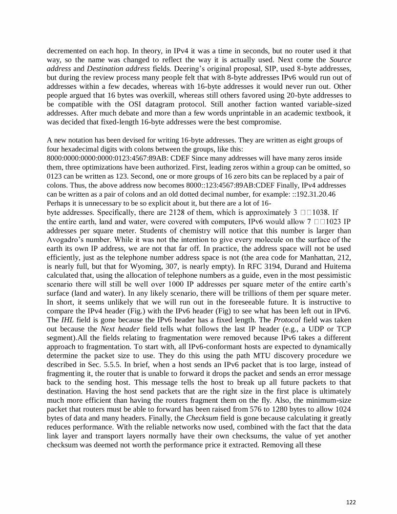
122
decremented on each hop. In theory, in IPv4 it was a time in seconds, but no router used it that
way, so the name was changed to reflect the way it is actually used. Next come the Source
address and Destination address fields. Deering’s original proposal, SIP, used 8-byte addresses,
but during the review process many people felt that with 8-byte addresses IPv6 would run out of
addresses within a few decades, whereas with 16-byte addresses it would never run out. Other
people argued that 16 bytes was overkill, whereas still others favored using 20-byte addresses to
be compatible with the OSI datagram protocol. Still another faction wanted variable-sized
addresses. After much debate and more than a few words unprintable in an academic textbook, it
was decided that fixed-length 16-byte addresses were the best compromise.
A new notation has been devised for writing 16-byte addresses. They are written as eight groups of
four hexadecimal digits with colons between the groups, like this:
8000:0000:0000:0000:0123:4567:89AB: CDEF Since many addresses will have many zeros inside
them, three optimizations have been authorized. First, leading zeros within a group can be omitted, so
0123 can be written as 123. Second, one or more groups of 16 zero bits can be replaced by a pair of
colons. Thus, the above address now becomes 8000::123:4567:89AB:CDEF Finally, IPv4 addresses
can be written as a pair of colons and an old dotted decimal number, for example: ::192.31.20.46
Perhaps it is unnecessary to be so explicit about it, but there are a lot of 16-
addresses per square meter. Students of chemistry will notice that this number is larger than
Avogadro’s number. While it was not the intention to give every molecule on the surface of the
earth its own IP address, we are not that far off. In practice, the address space will not be used
efficiently, just as the telephone number address space is not (the area code for Manhattan, 212,
is nearly full, but that for Wyoming, 307, is nearly empty). In RFC 3194, Durand and Huitema
calculated that, using the allocation of telephone numbers as a guide, even in the most pessimistic
scenario there will still be well over 1000 IP addresses per square meter of the entire earth’s
surface (land and water). In any likely scenario, there will be trillions of them per square meter.
In short, it seems unlikely that we will run out in the foreseeable future. It is instructive to
compare the IPv4 header (Fig.) with the IPv6 header (Fig) to see what has been left out in IPv6.
The IHL field is gone because the IPv6 header has a fixed length. The Protocol field was taken
out because the Next header field tells what follows the last IP header (e.g., a UDP or TCP
segment).All the fields relating to fragmentation were removed because IPv6 takes a different
approach to fragmentation. To start with, all IPv6-conformant hosts are expected to dynamically
determine the packet size to use. They do this using the path MTU discovery procedure we
described in Sec. 5.5.5. In brief, when a host sends an IPv6 packet that is too large, instead of
fragmenting it, the router that is unable to forward it drops the packet and sends an error message
back to the sending host. This message tells the host to break up all future packets to that
destination. Having the host send packets that are the right size in the first place is ultimately
much more efficient than having the routers fragment them on the fly. Also, the minimum-size
packet that routers must be able to forward has been raised from 576 to 1280 bytes to allow 1024
bytes of data and many headers. Finally, the Checksum field is gone because calculating it greatly
reduces performance. With the reliable networks now used, combined with the fact that the data
link layer and transport layers normally have their own checksums, the value of yet another
checksum was deemed not worth the performance price it extracted. Removing all these

123
features has resulted in a lean and mean network layer protocol. Thus, the goal of IPv6—a fast, yet flexible, protocol with plenty of address space—is met by this design.
Extension Headers Some of the missing IPv4 fields are occasionally still needed, so IPv6 introduces the concept of (optional) extension headers. These headers can be supplied to provide extra information, but
encoded in an efficient way. Six kinds of extension headers are defined at present, as listed in
Fig. Each one is optional, but if more than one is present they must appear directly after the fixed
header, and preferably in the order listed.
IPv6 extension headers
Some of the headers have a fixed format; others contain a variable number of variable-length
options. For these, each item is encoded as a (Type, Length, Value) tuple. The Type is a 1-byte
field telling which option this is. The Type values have been chosen so that the first 2 bits tell
routers that do not know how to process the option what to do. The choices are: skip the option;
discard the packet; discard the packet and send back an ICMP packet; and discard the packet but
do not send ICMP packets for multicast addresses (to prevent one bad multicast packet from
generating millions of ICMP reports). The Length is also a 1-byte field. It tells how long the
value is (0 to 255 bytes). The Value is any information required, up to 255 bytes. The hop-by-hop
header is used for information that all routers along the path must examine. So far, one option has
been defined: support of datagrams exceeding 64 KB. The format of this header is shown in.
When it is used, the Payload length field in the fixed header is set to 0.
The hop-by-hop extension header for large data grams (jumbo grams)
As with all extension headers, this one starts with a byte telling what kind of header comes next.
This byte is followed by one telling how long the hop-by-hop header is in bytes, excluding the
first 8 bytes, which are mandatory. All extensions begin this way. The next 2 bytes indicate that
this option defines the datagram size (code 194) and that the size is a 4-byte number. The last 4
bytes give the size of the datagram. Sizes less than 65,536 bytes are not permitted and will result
in the first router discarding the packet and sending back an ICMP error message. Datagram’s

124
using this header extension are called jumbo grams. The use of jumbo grams is important for
supercomputer applications that must transfer gigabytes of data efficiently across the Internet.
The destination options header is intended for fields that need only be interpreted at the
destination host. In the initial version of IPv6, the only options defined are null options for
padding this header out to a multiple of 8 bytes, so initially it will not be used. It was included to
make sure that new routing and host software can handle it, in case someone thinks of a
destination option some day. The routing header lists one or more routers that must be visited on
the way to the destination. It is very similar to the IPv4 loose source routing in that all addresses
listed must be visited in order, but other routers not listed may be visited in between. The format
of the routing header is shown in Fig.
The extension header for routing
The first 4 bytes of the routing extension header contain four 1-byte integers. The Next header
and Header extension length fields were described above. The Routing type field gives the format
of the rest of the header. Type 0 says that a reserved 32-bit word follows the first word, followed
by some number of IPv6 addresses. Other types may be invented in the future, as needed.
Finally, the Segments left field keeps track of how many of the addresses in the list have not yet
been visited. It is decremented every time one is visited. When it hits 0, the packet is on its own
with no more guidance about what route to follow. Usually, at this point it is so close to the
destination that the best route is obvious. The fragment header deals with fragmentation similarly
to the way IPv4 does. The header holds the datagram identifier, fragment number, and a bit
telling whether more fragments will follow.
THE TRANSPORT LAYER
THE TRANSPORT SERVICE
Services Provided to the Upper Layers The ultimate goal of the transport layer is to provide efficient, reliable, and cost-effective data
transmission service to its users, normally processes in the application layer. To achieve this, the
transport layer makes use of the services provided by the network layer. The software and/or
hardware within the transport layer that does the work is called the transport entity. The
transport entity can be located in the operating system kernel, in a library package bound into
network applications, in a separate user process, or even on the network interface card. The first
two options are most common on the Internet. The (logical) relationship of the network,
transport, and application layers is illustrated in Fig.

125
there are also two types of transport service. The connection-oriented transport service is similar
to the connection-oriented network service in many ways. In both cases, connections have three
phases: establishment, data transfer, and release. Addressing and flow control are also similar in
both layers. Furthermore, the connectionless transport service is also very similar to the
connectionless network service. However, note that it can be difficult to provide a connectionless
transport service on top of a connection-oriented network service, since it is inefficient to set up a
connection to send a single packet and then tear it down immediately afterwards. The obvious
question is this: if the transport layer service is so similar to the network layer service, why are
there two distinct layers? Why is one layer not Problems occur, that’s what? The users have no
real control over the network layer, so they cannot solve the problem of poor service by using
better routers or putting more error handling in the data link layer because they don’t own the
routers. The only possibility is to put on top of the network layer another layer that improves the
quality of the service. If, in a connectionless network, packets are lost or mangled, the transport
entity can detect the problem and compensate for it by using retransmissions. If, in a connection-
oriented network, a transport entity is informed halfway through a long transmission that its
network connection has been abruptly terminated, with no indication of what has happened to the
data currently in transit, it can set up a new network connection to the remote transport entity.
Using this new network connection, it can send a query to its peer asking which data arrived and
which did not, and knowing where it was, pick up from where it left off.
Transport Service Primitives To allow users to access the transport service, the transport layer must provide some operations
to application programs, that is, a transport service interface. Each transport service has its own
interface. In this section, we will first examine a simple (hypothetical) transport service and its
interface to see the bare essentials. In the following section, we will look at a real example. The
transport service is similar to the network service, but there are also some important differences.
The main difference is that the network service is intended to model the service offered by real
networks, warts and all. Real networks can lose packets, so the network service is generally
unreliable.

126
A quick note on terminology is now in order. For lack of a better term, we will use the term
segment for messages sent from transport entity to transport entity.TCP, UDP and other Internet
protocols use this term. Some older protocols used the ungainly name TPDU (Transport
Protocol Data Unit). That term is not used much anymore now but you may see it in older
papers and books the network entity similarly processes the packet header and then passes the
contents of the packet payload up to the transport entity. This nesting is illustrated in Fig. 6-3
Connection Establishment Establishing a connection sounds easy, but it is actually surprisingly tricky. At first glance, it
would seem sufficient for one transport entity to just send a CONNECTION REQUEST segment
to the destination and wait for a CONNECTION ACCEPTED reply. The problem occurs when
the network can lose, delay, corrupt, and duplicate packets. This behaviour causes serious
complications. Imagine a network that is so congested that acknowledgements hardly ever get
back in time and each packet times out and is retransmitted two or three times. Suppose that the
network uses datagrams inside and that every packet follows a different route. Some of the
packets might get stuck in a traffic jam inside the network and take a long time to arrive. That is,
they may be delayed in the network and pop out much later, when the sender thought that they
had been lost. The worst possible nightmare is as follows. A user establishes a connection with a
bank, sends messages telling the bank to transfer a large amount of money to the account of a
not-entirely-trustworthy person. Unfortunately, the packets decide to take the scenic route to the
destination and go off exploring a remote corner of the network. The sender then times out and
sends them all again. This time the packets take the shortest route and are delivered quickly so
the sender releases the connection.
Packet lifetime can be restricted to a known maximum using one (or more) of the following techniques: 1. Restricted network design.

127
2. Putting a hop counter in each packet.
3. Time stamping each packet.
The first technique includes any method that prevents packets from looping, combined with some
way of bounding delay including congestion over the (now known) longest possible path. It is
difficult, given that internets may range from a single city to international in scope. The second
method consists of having the hop count initialized to some appropriate value and decremented
each time the packet is forwarded. The network protocol simply discards any packet whose hop
counter becomes zero. The third method requires each packet to bear the time it was created,
with the routers agreeing to discard any packet older than some agreed-upon time. This latter
method requires the router clocks to be synchronized, which itself is a nontrivial task, and in
practice a hop counter is a close enough approximation to age.
TCP uses this three-way handshake to establish connections. Within a connection, a timestamp is
used to extend the 32-bit sequence number so that it will not wrap within the maximum packet
lifetime, even for gigabit-per-second connections. This mechanism is a fix to TCP that was
needed as it was used on faster and faster links. It is described in RFC 1323 and called PAWS
(Protection Against Wrapped Sequence numbers). Across connections, for the initial
sequence numbers and before PAWS can come into play, TCP originally use the clock-based
scheme just described. However, this turned out to have security vulnerability. The clock made it
easy for an attacker to predict the next initial sequence number and send packets that tricked the
three-way handshake and established a forged connection. To close this hole, pseudorandom
initial sequence numbers are used for connections in practice.
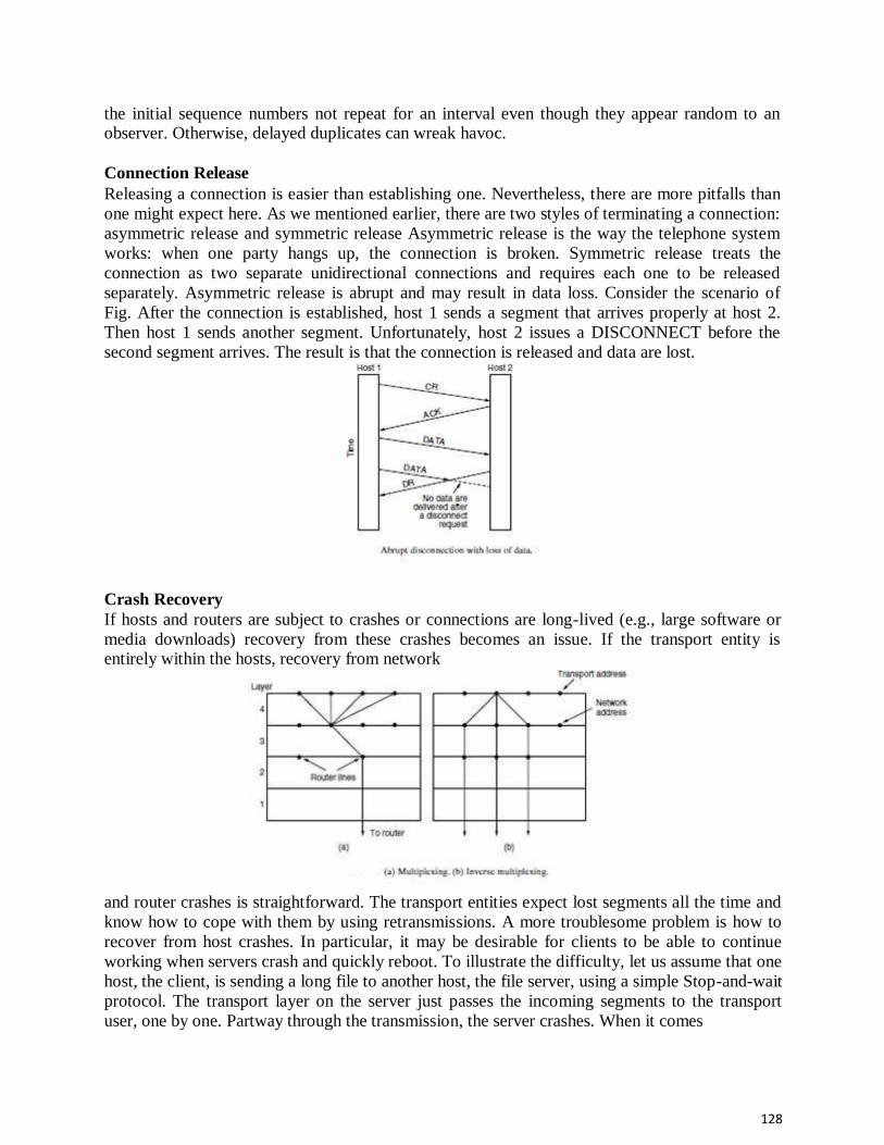
128
the initial sequence numbers not repeat for an interval even though they appear random to an observer. Otherwise, delayed duplicates can wreak havoc.
Connection Release Releasing a connection is easier than establishing one. Nevertheless, there are more pitfalls than
one might expect here. As we mentioned earlier, there are two styles of terminating a connection:
asymmetric release and symmetric release Asymmetric release is the way the telephone system
works: when one party hangs up, the connection is broken. Symmetric release treats the
connection as two separate unidirectional connections and requires each one to be released
separately. Asymmetric release is abrupt and may result in data loss. Consider the scenario of
Fig. After the connection is established, host 1 sends a segment that arrives properly at host 2.
Then host 1 sends another segment. Unfortunately, host 2 issues a DISCONNECT before the
second segment arrives. The result is that the connection is released and data are lost.
Crash Recovery If hosts and routers are subject to crashes or connections are long-lived (e.g., large software or
media downloads) recovery from these crashes becomes an issue. If the transport entity is entirely within the hosts, recovery from network
and router crashes is straightforward. The transport entities expect lost segments all the time and
know how to cope with them by using retransmissions. A more troublesome problem is how to
recover from host crashes. In particular, it may be desirable for clients to be able to continue
working when servers crash and quickly reboot. To illustrate the difficulty, let us assume that one
host, the client, is sending a long file to another host, the file server, using a simple Stop-and-wait
protocol. The transport layer on the server just passes the incoming segments to the transport
user, one by one. Partway through the transmission, the server crashes. When it comes

129
back up, its tables are reinitialized, so it no longer knows precisely where it was. In an attempt to
recover its previous status, the server might send a broadcast segment to all other hosts,
announcing that it has just crashed and requesting that its clients inform it of the status of all
open connections. Each client can be in one of two states: one segment outstanding, S1, or no
segments outstanding, S0. Based on only this state information, the client must decide whether to
retransmit the most recent segment.

130
UNIT-V
The Internet Transport Protocols, The Internet Transport Protocols and Application Layer
UDP Protocol UDP provides connectionless, unreliable, datagram service. Connectionless service means that there is no logical connection between the two ends exchanging messages. Each message is an
independent entity encapsulated in a datagram. UDP does not see any relation (connection) between consequent datagram coming from the same
source and going to the same destination. UDP has an advantage: it is message-oriented. It gives boundaries to the messages exchanged.
An application program may be designed to use UDP if it is sending small messages and the simplicity and speed is more important for the application than reliability.
User Datagram UDP packets, called user datagram, have a fixed-size header of 8 bytes made of four fields, each of 2 bytes (16 bits). . The 16 bits can define a total length of 0 to 65,535 bytes. However, the total length needs to be
less because a UDP user datagram is stored in an IP datagram with the total length of 65,535 bytes. The last field can carry the optional checksum
UDP Services
Process-to-Process Communication UDP provides process-to-process communication using socket addresses, a combination of IP addresses and port numbers.

131
Connectionless Services
As mentioned previously, UDP provides a connection less service. This means that each user
datagram sent by UDP is an independent datagram. There is no relationship between the
different user data grams even if they are coming from the same source process and going to the same destination program.
Flow Control UDP is a very simple protocol. There is no flow control, and hence no window mechanism. The receiver may overflow with incoming messages.
Error Control There is no error control mechanism in UDP except for the checksum. This means that the sender does not know if a message has been lost or duplicated.
Checksum UDP checksum calculation includes three sections: a pseudo header, the UDP header, and the data coming from the application layer. The pseudo header is the part of the header of the IP
packet in which the user datagram is to be encapsulated with some fields filled with 0s
UDP Applications
UDP Features
Connectionless Service As we mentioned previously,
UDP is a connectionless protocol. Each UDP packet is independent from other packets sent by the same application program. This feature can be considered as an advantage
or disadvanta8e depending on the application requirements.

132
UDP does not provide error control; it provides an unreliable service. Most
applications expect reliable service from a transport-layer protocol. Although a reliable
service is desirable.
Typical Applications The following shows some typical applications that can benefit more from the services of UDP
UDP is suitable for a process that requires simple request-response communication with little concern for flow and error control
UDP is suitable for a process with internal flow- and error-control mechanisms. For example, the Trivial File Transfer Protocol (TFIP)
UDP is a suitable transport protocol for multicasting. Multicasting capability is
embedded in the UDP software
UDP is used for management processes such as SNMP
UDP is used for some route updating protocols such as Routing Information Protocol (RIP)
UDP is normally used for interactive real-time applications that cannot tolerate
uneven delay between sections of a received message
TRANSMISSION CONTROL PROTOCOL
Transmission Control Protocol (TCP) is a connection-oriented, reliable protocol. TCP
explicitly defines connection establishment, data transfer, and connection teardown phases to
provide a connection-oriented service.
TCP Services
Process-to-Process Communication As with UDP, TCP provides process-to-process communication using port numbers. We have already given some of the port numbers used by TCP.
Stream Delivery Service In UDP, a process sends messages with predefined boundaries to UDP for delivery. UDP adds
its own header to each of these messages and delivers it to IP for transmission.
TCP, on the other hand, allows the sending process to deliver data as a stream of bytes and allows the receiving process to obtain data as a stream of bytes.
TCP creates an environment in which the two processes seem to be connected by an imaginary
"tube" that carries their bytes across the Internet.
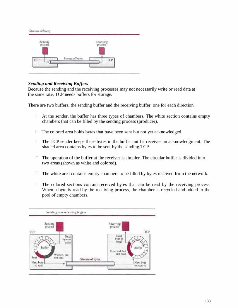
133
Sending and Receiving Buffers Because the sending and the receiving processes may not necessarily write or read data at the same rate, TCP needs buffers for storage.
There are two buffers, the sending buffer and the receiving buffer, one for each direction.
At the sender, the buffer has three types of chambers. The white section contains empty chambers that can be filled by the sending process (producer).
The colored area holds bytes that have been sent but not yet acknowledged.
The TCP sender keeps these bytes in the buffer until it receives an acknowledgment. The shaded area contains bytes to be sent by the sending TCP.
The operation of the buffer at the receiver is simpler. The circular buffer is divided into two areas (shown as white and colored).
The white area contains empty chambers to be filled by bytes received from the network.
The colored sections contain received bytes that can be read by the receiving process. When a byte is read by the receiving process, the chamber is recycled and added to the
pool of empty chambers.

134
Segments Although buffering handles the disparity between the speed of the producing and
consuming Processes, we need one more step before we can send data.
The network layer, as a service provider for TCP, needs to send data in packets, not as a stream of bytes. At the transport layer, TCP groups a number of bytes together into a
packet called a segment.
The segments are encapsulated in an IP datagram and transmitted. This entire operation is transparent to the receiving process.
Format The segment consists of a header of 20 to 60 bytes, followed by data from the application program. The header is 20 bytes if there are no options and up to 60 bytes if it contains options.
Source port address This is a 16-bit field that defines the port number of the application program in the host that is sending the segment.
Destination port address This is a 16-bit field that defines the port number of the application program in the host that is receiving the segment.
Sequence number This 32-bit field defines the number assigned to the first byte of data contained in this segment.

135
Acknowledgment number This 32-bit field defines the byte number that the receiver of the
segment is expecting to receive from the other party.
Header length This 4-bit field indicates the number of 4-byte words in the TCP header. The
length of the header can be between 20 and 60 bytes.
A TCP Connection
TCP is connection-oriented. a connection-oriented transport protocol establishes a
logical path between the source and destination.
All of the segments belonging to a message are then sent over this logical path.
TCP operates at a higher level. TCP uses the services of IP to deliver individual
segments to the receiver, but it controls the connection itself.
In TCP, connection-oriented transmission requires three phases: connection
establishment, data transfer, and connection termination.
Connection Establishment
TCP transmits data in full-duplex mode. When two TCPs in two machines are connected,
they are able to send segments to each other simultaneously.
Three- Way Handshaking The connection establishment in TCP is called three-way handshaking. an application program, called the client, wants to make a connection with another application program, called the server,

136
using TCP as the transport-layer protocol The process starts with the server. The server program
tells its TCP that it is ready to accept a connection. This request is called a passive open.
Although the server TCP is ready to accept a connection from any machine in the world, it cannot make the connection itself.
The client program issues a request for an active open. A client that wishes to connect to an open server tells its TCP to connect to a particular server.
A SYN segment cannot carry data, but it consumes one sequence number.
A SYN + ACK segment cannot carry data, but it does consume one sequence number.
An ACK segment, if carrying no data, consumes no sequence number.

137
HTTP The Hyper Text Transfer Protocol (HTTP) is used to define how the client-server programs can be written to retrieve web pages from the Web.
An HTTP client sends a request; an HTTP server returns a response. The server uses the port number 80; the client uses a temporary port number.
Non persistent versus Persistent Connections If the web pages, objects to be retrieved, are located on different servers, we do not have any
other choice than to create a new TCP connection for retrieving each object. If some of the
objects are located on the same server, we have two choices: to retrieve each object using a new
TCP connection
Non persistent Connections In a non persistent connection, one TCP connection is made for each request/response. The following lists the steps in this strategy:
1. The client opens a TCP connection and sends a request.
2. The server sends the response and closes the connection. 3. The client reads the data until it encounters an end-of-file marker; it then closes the connection.

138
Persistent Connections
HTTP version 1.1 specifies a persistent connection by default. In a persistent connection, the server leaves the connection open for more requests after sending a response.
The server can close the connection at the request of a client or if a time-out has been reached. The sender usually sends the length of the data with each response.

139
Message Formats
The first section in the request message is called the request line; the first section in the response message is called the status line.
The other three sections have the same names in the request and response messages.
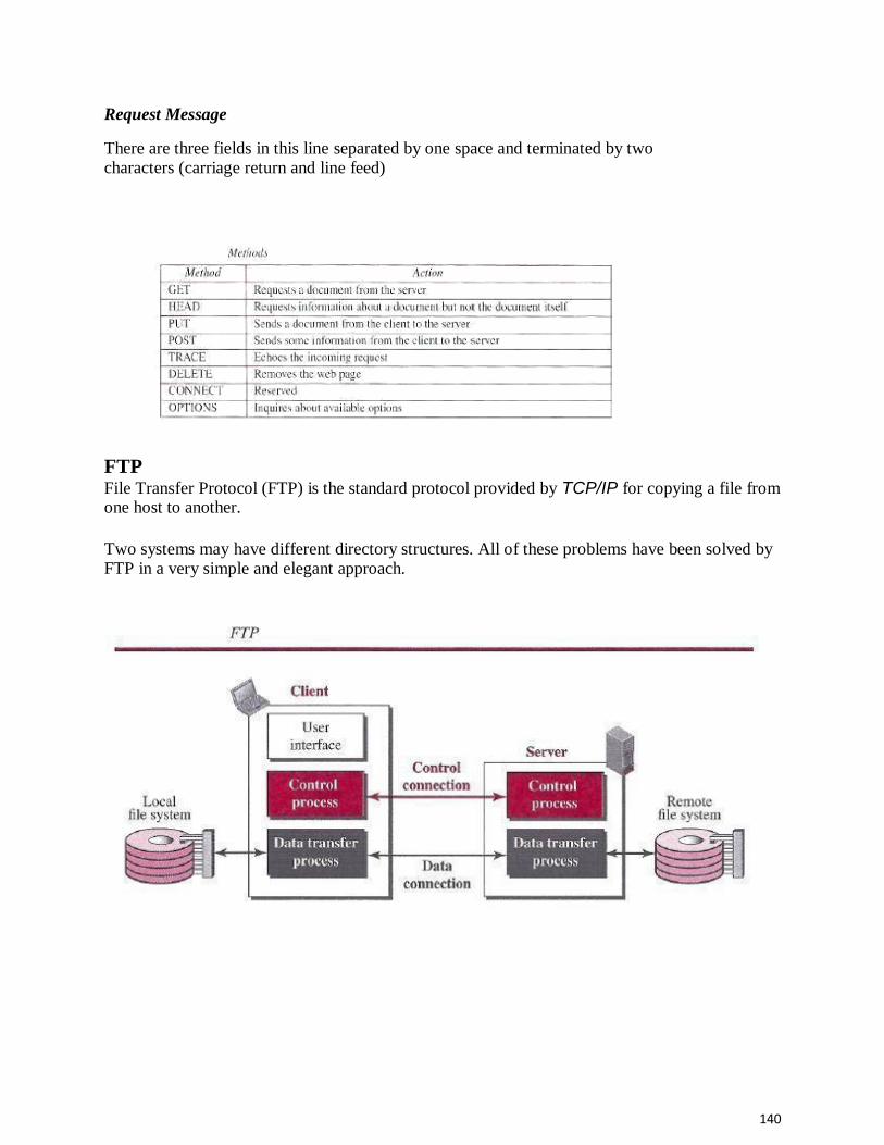
140
Request Message
There are three fields in this line separated by one space and terminated by two characters (carriage return and line feed)
FTP File Transfer Protocol (FTP) is the standard protocol provided by TCP/IP for copying a file from one host to another.
Two systems may have different directory structures. All of these problems have been solved by FTP in a very simple and elegant approach.

141
Two Connections
The control connection remains connected during the entire interactive FTP session.
When a user starts an FTP session, the control connection opens. While the control
connection is open, the data connection can be opened and closed multiple times if
several files are transferred.
FTP uses two well-known TCP ports: port 21 is used for the control connection, and port
20 is used for the data connection.
ELECTRONIC MAIL Electronic mail (or e-mail) allows users to exchange messages.
In an application such as HTTP or FTP, the server program is running all the
time, waiting for a
request from a client.
When the request arrives, the server provides the service. There is a request and there is
a response.
In the case of electronic mail, the situation is different. First, e-mail is considered a
one-way transaction
The users run only client programs when they want and the intermediate servers apply
the client/server paradigm.
Architecture
In the common scenario, the sender and the receiver of the e-mail, are connected via
a LAN or a WAN to two mail servers.
The administrator has created one mailbox for each user where the received messages
are stored
A mailbox is part of a server hard drive, a special file with permission restrictions.

142
Only the owner of the mailbox has access to it. The administrator has also created
a queue (spool) to store messages waiting to be sent.
A simple e-mail use three different agents: a user agent (UA), a message transfer
agent (MTA), and a message access agent (MAA).
TELNET One of the original remote logging protocols is TELNET, which is an abbreviation for Terminal
Network. A hacker can eavesdrop and obtain the logging name and password. Because of this security
issue, the use of TELNET has diminished in favor of another protocol, Secure Shell (SSH),
Local versus Remote Logging
When a user logs into a local system, it is called local logging. As a user types at a terminal or at a workstation running a terminal emulator, the keystrokes are accepted by the terminal driver.
When a user wants to access an application program or utility located on a remote machine, she performs remote logging.
The characters are sent to the TELNET client, which transforms the characters into a universal character set called Network Virtual Terminal (NVT) characters

143
Network Virtual Terminal (NVT)
The mechanism to access a remote computer is complex. This is because every computer and its
operating system accept a special combination of characters as tokens .We is dealing with
heterogeneous systems. If we want to access any remote computer in the world TELNET solves this problem by defining a universal interface called the Network Virtual Terminal (NVT)
character set. The server TELNET, on the other hand, translates data and commands from NVT form into the form acceptable by the remote computer.
SECURE SHELL (SSH)
Secure Shell (SSH) is a secure application program that can be used today for several purposes such as remote logging and file transfer; it was originally designed to replace TELNET.
There are two versions of SSH: SSH-l and SSH-2

144
Components
SSH Transport-Layer Protocol (SSH-TRANS)
SSH first uses a protocol that creates secured channel on top of the TCP.
When the procedure implementing this protocol is called, the client and server first use the TCP protocol to establish an insecure connection.
SSH Authentication Protocol (SSH-AUTH)
After a secure channel is established between the client and the server and the server is
authenticated for the client
SSH can call another procedure that can authenticate the client for the server. The client
authentication process in SSH is very similar to what is done in Secure Socket Layer
(SSL)
The request includes the user name, server name, the method of authentication, and the
required data.
The server responds with either a success message, which confirms that the client is authenticated, or a failed message
SSH Connection Protocol (SSH-CONN) One of the services provided by the SSH-CONN protocol is multiplexing. SSH-CONN takes the secure channel established by the two previous protocols and lets the client create multiple
logical channels over it. Each channel can be used for a different purpose, such as remote logging, file transfer, and so on

145
DOMAIN NAME SYSTEM (DNS)
The host that needs mapping can contact the closest computer holding the needed information. This method is used by the Domain Name System (DNS).
A user wants to use a file transfer client to access the corresponding file transfer server running on a remote host.
The user knows only the file transfer server name, such as afilesource.com.
Name Space
A name space that maps each address to a unique name can be organized in two ways: flat
or hierarchical. In a flat name space, a name is assigned to an address. A name in this space is a sequence
of characters without structure. In a hierarchical name space, each name is made of several parts.

146
Domain Name Space
Domain Name Space To have a hierarchical name space, a domain name space was designed. In this design the names are defined in an inverted-tree structure with the root at the top.
Label Each node in the tree has a label, which is a string with a maximum of 63 characters. The root label is a null string (empty string).
Domain Name
If a label is terminated by a null string, it is called a fully qualified domain name (FQDN).
If a label is not terminated by a null string, it is called a partially qualified domain name PQDN).
Domain A domain is a sub tree of the domain name space. The name of the domain is the name of the node at the top of the sub tree.

147
Distribution of Name Space
The information contained in the domain name space must be stored.
However, it is very inefficient and also not reliable to have just one computer store such a huge amount of information. It is inefficient because responding to requests from all over the world
places a heavy load on the system it is not reliable because any failure makes the data
inaccessible.

148
Zone
Since the complete domain name hierarchy cannot be stored on a single server, it is divided
among many servers. What a server is responsible for or has authority over is called a zone. The server makes a database called a zone file and keeps all the information for every node under that domain.
Top Related