


Languages
Pages
Legal


Munich Personal RePEc Archive
Investigating impact of volatility
persistence, market asymmetry and
information inflow on volatility of stock
indices using bivariate GJR-GARCH
Sinha, Pankaj and Agnihotri, Shalini
Faculty of Management Studies, University of Delhi
28 July 2014
Online at https://mpra.ub.uni-muenchen.de/58303/
MPRA Paper No. 58303, posted 04 Sep 2014 08:29 UTC

1
Investigating impact of volatility persistence, market asymmetry and
information inflow on volatility of stock indices using bivariate GJR-GARCH
Pankaj Sinha and Shalini Agnihotri
Faculty of Management Studies,
University of Delhi
Abstract
Joint dynamics of market index returns, volume traded and volatility of stock market returns can
unveil different dimensions of market microstructure. It can be useful for precise volatility
estimation and understanding liquidity of the financial market. In this study, the joint dynamics is
investigated with the help of bivariate GJR-GARCH methodology given by Bollerslev (1990), as
this method helps in jointly estimating volatility equation of return and volume in one step
estimation procedure and it also eliminates the regressor problem (Pagan ,1984).Three indices of
different market capitalization have been considered where, S&P BSE Sensex represent large
capitalization firms, BSE mid-cap represents mid-capitalization firms and BSE small-cap index
represents small capitalization firms. The study finds that there exist negative conditional
correlation between volume traded and return of large cap index. There is unidirectional relation
between index returns and volume traded since change in volume can be explained by lags of
index returns. The relation between volume traded and volatility is found to be positive in case of
large-cap index but it is negative in the case of mid-cap and small-cap indices. It is observed that
there exist bidirectional causality between volatility and volume traded in all the three indices
considered. Volatility is affected by pronounced persistence in volatility, mean-reversion of
returns and asymmetry in market. The rate of information arrival measured by IDV(Intra-day
volatility) is found to be a significant source of the conditional heteroskedasticity in Indian
markets since the presence of volume (proxy for information flow) in volatility equation, as an
independent variable, marginally reduces the volatility persistence, whereas presence of IDV, as
a proxy for information flow, completely vanishes the GARCH effect. Finally, it is observed that

2
volume traded spills over from large cap to mid-cap index, from large-cap to small-cap index and
from mid-cap to small-cap index, in response to new information arrival.
Keyword: Bivariate GJR-GARCH, Trading volume, Volatility, Stock return, Volatility
Persistence, Asymmetry in markets
JEL Classification: C12, C32, G12
1. Introduction
In financial markets volatility is an important risk factor. Asset pricing models and portfolio
allocation methods rely on its precise estimation. Precision in volatility estimation can be
particularly useful for investment firms and risk management purposes. Volatility is affected by
pronounced persistence in volatility, mean-reversion of returns and asymmetry in market. In
recent times, stock markets across the world have been experiencing high levels of volatility.
Understanding dynamic relation among stock return, trading volume and volatility is of interest
to academicians and risk managers as this relation may lead to better forecasting of stock return
volatility and pricing of derivatives in Indian markets. There is growing body of literature that
suggest that use of volatility predicted from more sophisticated time-series models will lead to
more accurate option valuations, asset pricing, risk assessment and risk management. Secondly,
this understanding can lead to better estimation of the distribution of stock returns. Volatility
exhibits the phenomena of persistence i.e. clustering of large moves and small moves (of either
sign) in the price process, a well-documented feature of volatility of assets. Persistence in
variance of a random variable, evolving through time, refers to the property of momentum in
conditional variance. According to Lamoureux and Lastrapes (1990) daily returns are generated
by mixture of distributions, in which the rate of daily information arrival is the stochastic mixing
variable. Autoregressive conditional heteroskedasticity (ARCH) in daily stock return data
reflects time dependence in the process of generating information flow to the market. Daily
trading volume, used as a proxy for information arrival time, is shown to have significant
explanatory power regarding the variance of daily returns. The degree to which conditional
variance is persistent in daily stock return data is an important issue. Poterba and Summers
(1986) showed that the extent to which stock return volatility affects stock prices depends
critically on the permanence of shock to the variance. The implication of such volatility

3
clustering is that volatility shocks today will influence the expectation of volatility many periods
in the future. Volatility is defined as;
Let the expected value of the variance of returns k periods ahead in the future is represented as: ℎ𝑡+𝑘|𝑡 = 𝐸𝑡[(𝑟𝑡+𝑘 − 𝑚𝑡+𝑘) 2] (1)
Where ℎ𝑡+𝑘|𝑡 represents volatility k periods ahead conditioned on information set at t, 𝑟𝑡+𝑘 and 𝑚𝑡+𝑘 represents return and average return at 𝑡 + 𝑘 period, respectively. The forecast of future
volatility then will depend upon information in today’s information set such as today’s returns.
Volatility is said to be persistent if today’s return shock have large effect on the forecast variance
many periods ahead in the future.
Lamoureux & Lastrapes(1990) suggested volume traded of stocks can be taken as a proxy for the
information flow in the markets. If volume traded is acting as a proxy for information flow in the
markets then persistence in volatility can be reduced by incorporating volume in the volatility
equation, since information arrival into markets is one of the appealing theoretical explanations
for the presence of heteroskedasticity in the financial returns . According to Rozga & Arneric
(2009) when volatility persistence is high, reaction of volatility on past market movements are
low, and shocks in volatility disappears slowly. When volatility persistence is low, reaction of
volatility on past market movements are much intensive, and shocks in volatility disappears
quickly. The purpose of this study is to empirically examine the dynamic (causal) relation among
stock market returns, trading volume, and volatility of stock index returns. It also studies
volatility persistence and mean spillover of volume traded from large-cap to mid-cap index, from
mid-cap to small-cap index and vice versa. The asset pricing models do not have place for
volume data ( Ross, 1987), and researchers are still uncertain about the precise role of volume in
the analysis of financial markets as a whole, volume data may contain information useful for
modeling volatility or the returns themselves. By examining the dynamic relation between
volume and returns, one can study how the nature of investor heterogeneity determines the
behavior of asset pricing. It is shown that heterogeneity among investors give rise to different
volume behavior and return volume dynamics. This implies that trading volume conveys
important information about how assets are priced in the market.
4
Since volatility is affected by pronounced persistence in volatility, mean-reversion of returns and
asymmetry in market. It would be interesting to investigate the effect of predetermined variables
such as volume; Intra-day volatility and Overnight indicator that may influence the volatility as
these variables affect persistence in volatility. It is also important to analyze relation between
return and trading volume as it can provide insight into the structure of financial markets, as
stock prices are noisy which can’t convey all available information of market dynamics.
Therefore, studying the joint dynamics of stock price returns, trading volume, volatility and
volatility persistence is essential to improve the understanding of the volatility forecasting and
stock markets microstructure. The paper investigates this problem in subsequent six sections.
Section 2 acquaints the reader with the literature survey. Section 3 acquaints the reader with the
data and summary statistics. Section 4 describes the methodology used. Section 5 presents the
results and sections 6 concludes the study.
2. Literature Review
2.1 Trading volume and volatility
There are numerous studies which document the relationship between stock market trading
volume and return volatility. For example, Granger and Morgenstern (1963) investigated the
relation between price change and aggregate exchange trading volume. Crouch (1970) studied
relation between contemporaneous absolute price change and trading volume. Westerfield (1977)
Tauchen and Pitts (1983) and Rogalski (1978) documented relation between price change and
trading volume. Epps and Epps (1976) used transactions data from 20 stocks and they found a
positive relation between the variances of price changes and the trading volume levels.
Clark(1973) and Lamoureux and Lastrapes (1990, 1994) link price volatility with the underlying
information flow in the markets and use volume as a measure of the information flow.
Clark(1973) showed that the time series of market returns is not drawn from a single probability
distribution but rather from a mixture of conditional distributions with varying degrees of
efficiency in generating the expected return. The autoregressive mixing variable considered is
the rate at which information arrives at the market; it explains the presence of GARCH effects in
daily stock price movements. Further, trading volume is considered the standard proxy for this
mixing variable, trading volume and volatility must be positively correlated as they jointly
depend upon common underlying variable. This variable could be the rate at which information
5
flows to the market. Lamoureux and Lastrapes(1990) gave Mixture of Distributions Hypothesis
(MDH), they studied the empirical relation between volume and volatility of stocks, they used
econometric framework to test whether there are GARCH effects remaining after the conditional
volatility specification includes the contemporaneous trading volume, which is a proxy for
information arrival. They find that for individual stocks, volatility persistence falls significantly
once contemporaneous trading volume is included in the volatility equation. Support for MDH is
large Gallo and Pacini (2000) used Volume, Intra-day volatility (IDV) and overnight indicator
(ONI) as proxy for information arrival. Kim and Kon (1994) provide support for this notion in
U.S. stock markets while evidence is found in U.K. stock markets by Omran and McKenzie
(2000). With respect to less developed markets, Pyun, Lee, and Nam (2000) provide positive
evidence from the Korean stock market; Bohl and Henke (2003) showed support from the Polish
stock market, while Lucey (2005) finds mixed evidence for the MDH in the Irish stock market.
The results contradicting the findings of Lamoureux and Lastrapes (1990) are Chen (2001),
Chen, Firth, and Rui (2001).
Chen (2001) investigated volume effects in the context of an EGARCH model and found that,
volatility persistence remains across the nine national markets in their sample. Chen, Firth, and
Rui (2001) said persistence in volatility is not eliminated when lagged or contemporaneous
trading volume is incorporated into the GARCH model.
The second set of information based models, given by Copeland (1976) and Jennings, Starks,
and Fellingham (1981), assume asymmetric dissemination of information. They said new
information is disseminated sequentially to traders, and uninformed traders cannot infer the
presence of informed traders perfectly. Informed traders take positions and adjust their portfolios
accordingly, resulting in a series of sequential equilibrium before a final equilibrium is attained.
This sequential dissemination of information from trader to trader is correlated with the number
of transactions. Consequently, new arrival of information to the market results not only in price
movements but also a rise in trading volume. Further, rise in information shocks generates
increases in both trading volume and price movements.
The third set of information based model is given by Harris and Raviv (1993) known as,
Difference of Opinions theory they assumed that investors are homogenous with respect to their
prior beliefs and the new information they receive. However, where investors differ from one

6
another is in their beliefs about the effect of new public information on asset prices. The
asymmetry in their interpretation of the common information drives investors to speculative
trading and this result in trading volume and absolute price changes being positively correlated.
Admati and Pfleiderer (1988) documented that, volume and price movements are clustered in
time because traders who have the choice of timing their trades at their discretion choose to trade
when recent volume is large. Their multi-period model assumes that traders are motivated by
either information or liquidity. All traders do not share the same information and informed
trader’s trade when they have some private information. On the other hand, liquidity or noise
traders are motivated by factors other than expected payoffs through future price movements. For
instance, some institutional traders may be trading due to liquidity needs of their clients.
Irrespective of the trader’s motivation, both information and liquidity have some discretion
regarding the timing of their trades leading to endogenously determined trading patterns. This
strategic timing of trading partially explains the positive relation between trading volume and the
variability of stock returns.
2.2 Trading volume and stock return
Osborne (1959) studied the return and volume relation from a variety of perspectives. Silvapulle
and Choi (1999) used daily Korean composite stock index data to study the linear and nonlinear
Granger causality between stock price and trading volume, and find a significant causality
between the two series. Ranter and Leal (2001) examine the Latin American and Asian financial
markets they find a positive contemporaneous relation between return and volume in all of the
countries in their sample except India. Chen, Firth, and Rui (2001) find mixed results of the
causality between price and volume. Similarly, Lee and Rui (2002) do not find evidence of
trading volume to predict stock returns in four Chinese stock exchanges. Chordia and
Swaminathan (2000) studied the interaction between trading volume and the predictability of
short-term stock returns. They find that, daily returns of stocks with high trading volume lead
daily returns of stocks with low trading volume. They attribute this empirical result to the
tendency of high volume stocks to respond promptly to market-wide information. Chordia and
Swaminathan said that trading volume plays an important role in market wide information
dissemination. According to Chordia, Huh, and Subrahmanyam (2006) past returns are the most
significant predictor of turnover and find that higher positive and negative returns lead to

7
substantially higher turnover. Hiemstra and Jones (1994) studied dynamic relation between stock
return and percentage change in trading volume using Granger causality. Jain and Joh (1988),
used intraday data from a market index they find a similar correlation over one hour intervals.
Gallant, Rossi, and Tauchen (1992) examined the relation between S&P 500 index returns and
trading volume in the NYSE and find evidence of returns leading trading volume. Using data
from stocks traded on the NYSE. Gervais and Mingelgrin (2001) report that period of high
trading volume tend to be followed by periods of positive excess returns whereas periods of low
volume tend to be followed by negative excess returns. These findings also suggest that a
positive relation exists between returns and trading volume and that returns precedes volume.
He and Wang (1995) develop a rational expectations model of stock trading in which investors
have different information concerning the underlying value of the stock. They examined the way
in which trading volume relates to the information flow in the market, and how investors’ trading
reveals their private information. Their model shows how over time, trading volume is closely
related to the flow and nature of information in the market. They developed a multi-period model
with heterogeneous investors and differential information. Investors have asymmetric private and
public information and trade competitively based on this asymmetry. Chuang (2012) studied the
contemporaneous and causal relation between stock return, trading volume and volatility in ten
Asian stock markets using bivariate GJR-GARCH model. They documented positive relation
between trading volume and stock returns but mixed results for trading volume and volatility of
stock indexes.
3. Data and summary statistics
S&P BSE Sensex 30, BSE mid-cap index and BSE small-cap index have been considered for
analysis. Daily closing, open, high, low price and volume traded of indices are taken from
Bloomberg database. The data covers sample period from January 6th, 2005 to December 31st,
2013. Daily log returns are calculated on adjusted closing price of indices. According to Lo and
Wang (2000), log of volume (number of shares traded in a day) is taken as a measure of raw
trading volume. The studies by Gallant, Rossi, and Tauchen (1992), Lo and Wang (2000), Chen
(2001) and Chuang (2012) reported strong evidence of both linear and nonlinear time trends in
trading volume series. We tested trend stationary in trading volume by regressing the series on a
deterministic function of time. For all the three indices, log volume is regressed on linear and

8
quadratic deterministic time trend in equation (2) to make the volume series stationary by
detrending. In case of Sensex, the log volume series is found to have significant linear
deterministic time trend. Therefore, the residuals of linear time trend regression is used as
detrended volume. Whereas, in the case of mid-cap and small-cap index both linear and
quadratic time trend are found to be highly significant therefore, regression residuals of linear
and quadratic time trend are used as detrended volume. Following regression is used to obtain
detrended volume series. 𝑣𝑡 = 𝛼 + 𝛽1 𝑡 + 𝛽2𝑡2 + 𝜀𝑡 (2)
Where, 𝑣𝑡 is natural log volume traded in a day in each stock market index.
Apart from considering detrended trading volume, we have also considered IDV (Intra- day
volatility) and ONI (Over-night indicator) measure used as a proxy for information flow for the
indices considered.
Table 1 Summary Statistic
Summary statistic
Index Large cap Mid Cap Small Cap Index Large cap Mid Cap Small Cap
Panel A: Return series Panel B: Detrended trading volume
Observations 2233 2233 2233 Observations 2233 2233 2233
Mean 0.000532 0.000363 0.000296 Mean 1.92E-18 7.16E-19 7.60E-19
Median 0.00101 0.001871 0.002163 Median 0.000183 0.000189 9.24E-05
Maximum 0.1599 0.111113 0.086601 Maximum 1.77E-02 8.31E-03 3.61E-03
Minimum -0.116044 -0.120764 -0.108357 Minimum 0.005739 0.001734 0.00114
Std. Dev. 0.016301 0.015311 0.015748 Std. Dev. 0.002084 9.10E-04 0.000595
Skewness 0.097264 -0.838204 -0.893373 Skewness 1.776526 3.30059 1.250894
Kurtosis 10.48405 10.04302 7.917771 Kurtosis 11.06623 19.80929 5.941447
Jarque-Bera 5214.882*** 4876.734*** 2547.195*** Jarque-Bera 7228.241*** 30343.46*** 1387.349***
LB-Q(8) 479.59*** 814.09*** 848.54*** LB-Q(8) 933.26*** 6092.2*** 3006.2***
LB-Q(11) 693.96*** 894.34*** 946.72*** LB-Q(11) 1074*** 7128.7*** 3276.7***
LM
TEST(10) 2.904641*** 12.62611*** 22.78948***
LM
TEST(10) 329.8837*** 1309.989*** 657.3763***
ARCH(10) 31.82867*** 53.89687*** 50.36925*** ARCH(10) 49.65657*** 813.864*** 185.4702***
ADF Test (43.9121)*** (38.28912)*** (35.30004)*** ADF Test (7.454505)*** (4.605358)*** (7.758133)***
KPSS 0.151109 0.131038 0.161893 KPSS 0.353791 0.230517 0.139288
Note:
Critical values of KPSS test at 1%, 5% and 10% are 0.739,0.463,0.347 respectively
***,**.* denote significance at 1%,5% and 10% respectively. Negative values are represented in brackets ( )
LB-Q is Ljung–Box test for autocorrelation with number of lags in brackets.
ADF stands for Augmented Dicky Fuller test, which has null hypothesis that series has unit root.
KPSS stands for Kwiatkowski Phillips Schmidt Shin test, which has null hypothesis that series does not have unit root,
Time Period considered for the analysis is from January 6th, 2005 till December 31st, 2013.
LM test is Lagrange multiplier test for serial correlation, which has null hypothesis of no serial correlation among lags.
ARCH test is used for checking heteroskedasticity in data, which has null hypothesis of homoscedasticity.

9
From Table 1, it is observed that mean returns are decreasing with decreasing market
capitalization. Daily standard deviation of returns is highest in Sensex. Sensex returns are
positively skewed and all the three indices show kurtosis more than three. The kurtosis value is
decreasing with decrease in market capitalization. Jarque-Bera test statistics is significant for all
the three indices, indicating that the stock indices returns are not normally distributed. Ljung-
Box statistics is highly significant for all the three indices considered in the study, indicating the
presence of autocorrelation in all the sample indices. The autocorrelation was found much
stronger in mid-cap and small-cap indices returns than in Sensex. Engle ARCH LM(Lagrange
multiplier) test with 10 lags was applied to test the presence of ARCH effect and time varying
volatility. The LM test statistics is highly significant at 5% level, indicating the presence of
heteroskedasticity in all the three indices considered. Therefore, GARCH family models were
used to model the heteroskedasticity. Further, Engle and Ng (1993) tests were used to check
asymmetry in volatility. Sign bias test examines the impact of asymmetric response of positive
and negative return shocks on volatility. Negative sign bias test examines different effects that
large and small negative return shocks have on volatility which is not predicted by the GARCH
specification. Positive sign bias test examines different effects that large and small positive
return shocks have on volatility which is not predicted by the GARCH specification. Engle and
Ng test involves estimating a GARCH (1, 1) model in the first stage; then the estimated
standardized squared residuals �̂�𝑡2 is used in following regression:
Sign bias test: �̂�𝑡2 = 𝜆0 + 𝜆1 𝑠𝑡−1− + 𝜈𝑡 (3)
Negative size bias test: �̂�𝑡2 = 𝜆0 + 𝜆1 𝑠𝑡−1− �̂� 𝑡−1 + 𝜈𝑡 (4)
Positive size bias test: �̂�𝑡2 = 𝜆0 + 𝜆1 𝑠𝑡−1+ �̂� 𝑡−1 + 𝜈𝑡 (5)
Where 𝑠𝑡−1− is an indicator dummy variable that takes value of 1 if, �̂� 𝑡−1<0 (bad news) and 0
otherwise and 𝑠𝑡−1+ =1-𝑠𝑡−1− that takes value of 1 if, �̂� 𝑡−1>0 (good news) and 0 otherwise.
10
Table 2
Engle and Ng test on residuals of GARCH model(test for asymmetry)
Large
cap Estimate
Mid
cap Estimate
Small
cap Estimate
SBT (0.217543)*** SBT (0.378391)*** SBT (0.374575)***
NSBT 0.193765*** NSBT 0.264308*** NSBT 0.246405***
PSBT (0.195806)*** PSBT 0.32674*** PSBT 0.259524*** Note:
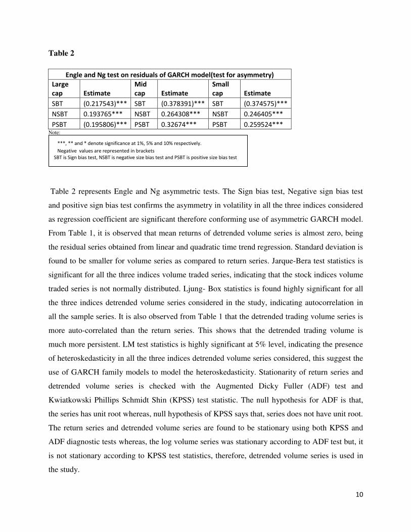
Table 2 represents Engle and Ng asymmetric tests. The Sign bias test, Negative sign bias test
and positive sign bias test confirms the asymmetry in volatility in all the three indices considered
as regression coefficient are significant therefore conforming use of asymmetric GARCH model.
From Table 1, it is observed that mean returns of detrended volume series is almost zero, being
the residual series obtained from linear and quadratic time trend regression. Standard deviation is
found to be smaller for volume series as compared to return series. Jarque-Bera test statistics is
significant for all the three indices volume traded series, indicating that the stock indices volume
traded series is not normally distributed. Ljung- Box statistics is found highly significant for all
the three indices detrended volume series considered in the study, indicating autocorrelation in
all the sample series. It is also observed from Table 1 that the detrended trading volume series is
more auto-correlated than the return series. This shows that the detrended trading volume is
much more persistent. LM test statistics is highly significant at 5% level, indicating the presence
of heteroskedasticity in all the three indices detrended volume series considered, this suggest the
use of GARCH family models to model the heteroskedasticity. Stationarity of return series and
detrended volume series is checked with the Augmented Dicky Fuller (ADF) test and
Kwiatkowski Phillips Schmidt Shin (KPSS) test statistic. The null hypothesis for ADF is that,
the series has unit root whereas, null hypothesis of KPSS says that, series does not have unit root.
The return series and detrended volume series are found to be stationary using both KPSS and
ADF diagnostic tests whereas, the log volume series was stationary according to ADF test but, it
is not stationary according to KPSS test statistics, therefore, detrended volume series is used in
the study.
***, ** and * denote significance at 1%, 5% and 10% respectively.
Negative values are represented in brackets
SBT is Sign bias test, NSBT is negative size bias test and PSBT is positive size bias test

11
4. Methodology
Lamourex and Lastrapes (1990) assumes that the volume is weakly exogenous with respect to
the returns, which is possibly a strong hypothesis. If the price movements within the day go
mainly in one direction creating a local trend, they may attract further trades and therefore affect
the volume. Therefore, to better understand the dynamics associated with the volume and
volatility we have used Bivariate GJR-GARCH methodology using conditional constant
correlation model of Bollerslev (1990).In this study, the joint dynamics is investigated with the
help of bivariate GJR- GARCH methodology given by Bollerslev (1990), as this method helps in
jointly estimating volatility equation of return and volume in one step estimation procedure and it
also eliminates the regressor problem (Pagan ,1984)Bollerslev and Wooldridge (1992) showed
that, GARCH parameters are consistently estimated by Gaussian maximum likelihood even
when normality assumption is violated. Bollerslev et al. (1988) proposed VECH model of
multivariate GARCH methodology major drawbacks of the VECH model are the difficulty to
guaranty a positive definite variance covariance matrix. This model was followed by the
Constant Conditional Correlation (CCC) model, proposed by Bollerslev (1990) with only
drawback is the assumption of constant correlations which is often unrealistic in empirical
applications. In this study Constant Conditional Correlation (CCC) model is used.
Bollerslev (1990) specifies the elements of the conditional covariance matrix as follows:
ℎ𝑖𝑖𝑡 = 𝑐𝑖 + 𝑎𝑖𝜀𝑖𝑡−12 + 𝑑𝑖𝐼𝑖𝑡−1− 𝜀𝑖𝑡−12 + 𝑏𝑖ℎ𝑖𝑖𝑡−1 (6)
ℎ𝑖𝑗𝑡 = 𝜌𝑖𝑗√ℎ𝑖𝑖𝑡ℎ𝑗𝑗𝑡 (7)
Where, ℎ𝑖𝑖𝑡 represents variance of asset 𝑖 at time t conditioned on the information set of asset 𝑖 and 𝜌𝑖𝑗 represents correlation between asset i and j, 𝑎𝑖, 𝑑𝑖 and 𝑏𝑖 represents coefficient of ARCH
term, asymmetric term and GARCH term respectively.
Let 𝑦𝑡 denote 𝑁 × 1 time-series vector of interest with time varying conditional covariance
matrix𝐻𝑡 , i.e. 𝑦𝑡 = 𝐸(𝑦𝑡|𝜓𝑡−1) + 𝜖𝑡 (8) 𝑉𝑎𝑟(𝜖𝑡|𝜓𝑡−1) = 𝐻𝑡
Where,𝜓𝑡−1is the σ field generated by all the available information up through time t - 1, and 𝐻𝑡is almost surely positive definite for all t. Also, let ℎ𝑖𝑗𝑡 denote the ijth element in Ht and 𝑦𝑖𝑡and

12
𝜖𝑖𝑡 the ith element in 𝑦𝑡 and 𝜖𝑡 respectively. Then a natural scale invariant measure of the
coherence between yit and yjt evaluated at time t - 1 is given by the conditional correlation.ℎ𝑖𝑗𝑡 =𝜌𝑖𝑗𝑡√ℎ𝑖𝑖𝑡ℎ𝑗𝑗𝑡 . An appealing feature of the model with constant conditional correlations relates
directly to the simplified estimation and inference procedures. To that end, rewrite each of the
conditional variances as, ℎ𝑖𝑖𝑡 = 𝜔𝑖𝜎𝑖𝑡2𝑖 = 1, … … . , 𝑁
With 𝜔𝑖 is a positive time invariant scalar and 𝜎𝑖𝑡2 > 0
the full conditional covariance matrix, Ht, may be partitioned as 𝐻𝑡 = 𝐷𝑡Γ𝐷𝑡 where, 𝐷𝑡 denotes 𝑁 × 𝑁stochastic diagonal matrix with elements 𝜎1𝑡, … … . . 𝜎𝑁𝑡 and Γ is 𝑁 × 𝑁time invariant
matrix with typical element 𝜌𝑖𝑗√𝜔𝑖𝜔𝑗.
ARCH estimation uses maximum likelihood to jointly estimate the parameters of the mean and
the variance equations. Assuming multivariate normality, the log likelihood contributions for
GARCH models is given by:
𝐿(𝜃) = − 𝑇𝑁2 𝑙𝑜𝑔(2𝜋) − 12 ∑ (𝑙𝑛|𝐻𝑡| + 𝜀𝑡′𝐻𝑡−1𝜀𝑡𝑇𝑡=1 ) (9)
Where, θ denotes all the unknown parameters to be estimated in𝜀𝑡 𝑎𝑛𝑑 𝐻𝑡, N is the number of
assets (i.e. the number of series in the system) and T is the number of observations. The
maximum likelihood estimate for θ is asymptotically normal, and thus traditional procedures for
statistical inference are applicable. Numerical optimization algorithm of Marquardt is used to
maximize this non-linear log likelihood function.
Volume is also affected by within the day price movements and it is not weakly exogenous
relative to returns, alternative proxies for information flow suggested by Gallo and Paccini
(2000) is also used in the study. The indicators are as follows:
4.1 Overnight Indicator (ONI)
Returns are difference between adjusted closing price, the difference between the opening price
of a day and the closing price of the day before represents an interesting indicator of the number
of trades during the day therefore, it may act as a variable on the basis of which the decision to
trade during the day can be made. The difference between opening price of day t and closing of
day t-1 is likely to affect the trading during the day which results in an impact on the daily
volatility. As a result, it can capture the persistence in the conditional heteroskedasticity.
13
Therefore, it helps us in taking out the stock returns volatility the component which is due to the
surprise between open and previous close price. By doing so, persistence in the estimated
volatility can be reduced. It is calculated as follows: 𝑂𝑁𝐼 = log (𝑜𝑝𝑒𝑛𝑡 𝑐𝑙𝑜𝑠𝑒𝑡−1⁄ ) (10)
4.2 Intra-day volatility (IDV)
IDV is calculated as the difference between the highest and the lowest price divided by the
closing price. IDV is taken as an indicator of the vivaciousness of trade within the day. The IDV
is calculated as follows: 𝐼𝐷𝑉 = 𝑝𝑡ℎ−𝑝𝑡𝑙𝑝𝑡𝑐 (11)
Where, 𝑝𝑡 denotes the highest (ℎ), the lowest (𝑙), and the closing (𝑐) price on day t, respectively.
5. Result and analysis
Mean equations of index returns and trading volume is in the form of restrictive bi-variate Vector
autoregressive model (VAR) specification. It is used to test causality running between return and
volume. The contemporaneous relation is estimated with the help of correlation coefficient
estimated from conditional multivariate GARCH specification. Short run causality between
volume and return of indices is tested with the help of Wald’s test. Examination of causality in
VAR will suggest source of return spillovers. The Chi-square test followed by Wald will not by
construction, be able to explain how long these effects will last, therefore VAR impulse
responses are also used in the study. Lag lengths of the mean equations are determined
using Akaike information criterion (AIC). Joint lag coefficients of volume and return are tested
using Wald’s coefficient test which follows Chi-square distribution with degree of freedom
equals to the lag length chosen. From Table 3 panel 2, the conditional mean equation of stock
index return it is evident that, lags of volume chi-square coefficient is not significant, therefore
null hypothesis of lagged index volume does not cause stock return is accepted. Therefore, it is
proved that lagged index volume does not cause stock index return, whereas lags of stock return
causes mean return as the Chi-square test statistic is found to be significant. Equations estimated
are as follows:

14
Mean equations:
𝑣𝑡 = 𝑐𝑣 + ∑ 𝜃𝑣,𝑖𝑣𝑣,𝑡−1𝑝𝑖=1 + ∑ 𝜇𝑣,𝑖𝑟𝑣,𝑡−1 𝑝𝑖=1 + 𝜀𝑣,𝑡 (12)
𝑟𝑡 = 𝑐𝑟 + ∑ 𝜃𝑟,𝑖𝑣𝑟,𝑡−1𝑝𝑖=1 + ∑ 𝜇𝑟,𝑖𝑟𝑟,𝑡−1 𝑝𝑖=1 + 𝜀𝑟,𝑡 (13)
Variance Equation:
𝜎𝑣,𝑡2 = 𝜔𝑣 + 𝛼𝑣𝜀𝑣,𝑡−12 + 𝛽𝑣𝜎𝑣,𝑡−12 + 𝜗𝑣𝑠𝑣,𝑡−1− (𝜀𝑣,𝑡−1 ) 2 (14)
𝜎𝑟,𝑡2 = 𝜔𝑟 + 𝛼𝑟𝜀𝑟,𝑡−12 + 𝛽𝑟𝜎𝑟,𝑡−12 + 𝜗𝑟𝑠𝑟,𝑡−1− (𝜀𝑟,𝑡−1 ) 2 + 𝜑𝑣𝑡 (15)
Variance Equation with ONI as indicator of information flow:
𝜎𝑟,𝑡2 = 𝜔𝑟 + 𝛼𝑟𝜀𝑟,𝑡−12 + 𝛽𝑟𝜎𝑟,𝑡−12 + 𝜗𝑟𝑠𝑟,𝑡−1− (𝜀𝑟,𝑡−1 ) 2 + 𝜑𝑟𝑂𝑁𝐼 (16)
Variance Equation with IDV as indicator of information flow:
𝜎𝑟,𝑡2 = 𝜔𝑟 + 𝛼𝑟𝜀𝑟,𝑡−12 + 𝛽𝑟𝜎𝑟,𝑡−12 + 𝜗𝑟𝑠𝑟,𝑡−1− (𝜀𝑟,𝑡−1 ) 2 + 𝜑𝑟 IDV (17)
Here subscript 𝑣 represent volume and subscript 𝑟 is for return of indices,𝑣𝑡 represents mean
volume traded, 𝜃𝑣,𝑖 is coefficient of lags of volume traded, 𝜇𝑣,𝑖 coefficients of lags of return on
indices in mean equation of volume traded.𝜃𝑟,𝑖 is coefficient of lags of volume traded in return
equation and 𝜇𝑟,𝑖 coefficients of lags of return on indices in mean equation of return. 𝑟𝑡represents
mean return of index. 𝜎𝑣,𝑡2 represents variance of volume traded and 𝜎𝑟,𝑡2 represents varianceof
mean returns of indices. 𝛼𝑣is ARCH term in volume equation, 𝛽𝑣 is GARCH coefficient in
volume equation and 𝜗𝑣 represents asymmetric term in volume equation. 𝜑𝑣𝑡represents,
contemporaneous volume traded in volatility equation of returns.𝛼𝑟 , 𝛽𝑟 and 𝜗𝑟 represents
ARCH term, GARCH term and asymmetric term in volatility equation of returns.
From Table 3 panel 1, it is evident that both lags of index return and lags of trading volume
causes volume. The results are same for all the three indices. Therefore we can say that, volume
follows return. Variance decomposition is also used in the study it gives the proportion of
variation of returns explained by returns itself and the proportion of variance in return explained

15
by volume and vice versa. The impulse response explains the response of returns to shocks in
returns and volume and vice versa. From fig 1 it is evident that, in case of Sensex response of
return to return die after two periods. Response of volume to volume lags is highly correlated
and it does not die after 10 periods. Response of volume to shock in return is not significant
according to impulse responses. Response of return to shock in volume is negative in case of
Sensex, until 2nd lag and it becomes positive after 3rd lag this explains the lead lag relationship
between return and volume. From fig 2, it is evident that, in case of mid-cap response of return to
return die after 5 periods. Response of volume to return dies after 20 periods. Response of return
to volume is almost zero. From fig 3, small-cap response of volume to return does not die after
20 lags. Therefore we can say that, with the decrease in market capitalization volume return lead
lag relationship is becoming stronger.

16
Table 3: Chi-square values for Wald test and coefficients of mean and variance equation of
volume traded and return of indices. The following GJR-GARCH model is estimated.
Lag length is chosen using Akaike information criterion (AIC). 𝑊𝜃𝑣,𝑖, 𝑊𝜇𝑣,𝑖 represents Wald test chi-square coefficients for volume equation
with degree of freedom equal to lag length chosen, it has null hypothesis that joint lag Wald coefficients is equal to zero.𝑊𝜃𝑟,𝑖 , 𝑊𝜇𝑟,𝑖 represents,
Wald test chi-square coefficients for mean equation.𝑣𝑡is trading volume at time t and 𝑟𝑡 is stock return at time t. subscript 𝑣 is for volume traded
equation and subscript r is for return of stock index equation. 𝑣𝑡 = 𝑐𝑣 + ∑ 𝜃𝑣,𝑖𝑣𝑣,𝑡−1𝑝𝑖=1 + ∑ 𝜇𝑣,𝑖𝑟𝑣,𝑡−1 𝑝𝑖=1 + 𝜀𝑣,𝑡 (12)
𝑟𝑡 = 𝑐𝑟 + ∑ 𝜃𝑟,𝑖𝑣𝑟,𝑡−1𝑝𝑖=1 + ∑ 𝜇𝑟,𝑖𝑟𝑟,𝑡−1 𝑝𝑖=1 + 𝜀𝑟,𝑡 (13)
𝜎𝑣,𝑡2 = 𝜔𝑣 + 𝛼𝑣𝜀𝑣,𝑡−12 + 𝛽𝑣𝜎𝑣,𝑡−12 + 𝜗𝑣𝑠𝑣,𝑡−1− (𝜀𝑣,𝑡−1 ) 2 (14)
𝜎𝑟,𝑡2 = 𝜔𝑟 + 𝛼𝑟𝜀𝑟,𝑡−12 + 𝛽𝑟𝜎𝑟,𝑡−12 + 𝜗𝑟𝑠𝑟,𝑡−1− (𝜀𝑟,𝑡−1 ) 2 + 𝜑𝑣𝑡 (15)
𝜎𝑟,𝑡2 = 𝜔𝑟 + 𝛼𝑟𝜀𝑟,𝑡−12 + 𝛽𝑟𝜎𝑟,𝑡−12 + 𝜗𝑟𝑠𝑟,𝑡−1− (𝜀𝑟,𝑡−1 ) 2 + 𝜑𝑟𝑂𝑁𝐼 (16)
𝜎𝑟,𝑡2 = 𝜔𝑟 + 𝛼𝑟𝜀𝑟,𝑡−12 + 𝛽𝑟𝜎𝑟,𝑡−12 + 𝜗𝑟𝑠𝑟,𝑡−1− (𝜀𝑟,𝑡−1 ) 2 + 𝜑𝑟 IDV (17)
Bivariate GJR-GARCH results
Index Large cap Mid cap Small cap
Panel 1: Conditional Mean equation Wald test results(trading volume)
Lag Length 10 10 7
Chi-square value 𝑊𝜃𝑣,𝑖 7577.091*** 10396.58*** 17673.45*** 𝑊𝜇𝑣,𝑖 32.05398*** 211.3163*** 205.362***
Panel:2 Conditional Mean equation Wald test results ( Stock index return)
Chi-square value 𝑊𝜃𝑟,𝑖 8.038562 6.884177 5.090475 𝑊𝜇𝑟,𝑖 29.21583*** 154.6224*** 193.2422***
Panel 3: Coefficients of conditional variance equation(Trading volume) 𝛼𝑣
0.030233***
[0.004232]
0.181516***
[0.014171]
0.213613***
[0.02171] 𝜗𝑣
0.042004***
[0.042004]
(0.112901)***
[0.015]
0.02403***
[0.036286] 𝛽𝑣
0.961711***
[0.0013]
0.868757***
[0.007811]
0.649845***
[0.0135]
Panel 4: Coefficients of variance equation with lagged volume ( Stock index return) 𝛼𝑟
0.022943***
[0.009789]
0.049736***
[0.011]
0.098258***
[0.012] 𝜗𝑟
0.140235***
[0.019967]
0.143988***
[0.019]
0.1122***
[0.021] 𝛽𝑟
0.888914***
[0.01067]
0.855942***
[0.009]
0.82357***
[0.010] 𝜑𝑉𝑡−1
0.000854***
[0.00025]
0.00235***
[0.0007]
0.002435**
[0.0010]
Log Likelihood 18923.94 21921.97 22178.51
17
Panel 5:Coefficients of variance equation without volume ( Stock index return)
Index Large cap Mid cap Small cap 𝛼𝑟
0.026701***
[0.010148]
0.054288***
[0.011]
0.103099***
[0.015] 𝜗𝑟
0.135474***
[0.019359]
0.140293***
[0.019]
0.111388***
[0.021] 𝛽𝑟
0.891188***
[0.010241]
0.855621***
[0.009]
0.817175***
[0.011]
Conditional
Correlation
(0.083521)***
[0.023]
0.089***
[0.0211]
0.116467***
[0.018]
Log Likelihood 18919.56 21913.18 22176.44
Panel 6: Coefficients of variance equation with contemporaneous volume (Stock index return) 𝛼𝑟
0.021575***
[0.009964]
0.048795***
[0.011314]
0.097267***
[0.014049] 𝜗𝑟
0.151828***
[0.21288]
0.14485***
[0.019597]
0.113409***
[2.16E-02] 𝛽𝑟
0.882469***
[0.011469]
0.856545***
[0.009253]
0.824417***
[0.01118] 𝜑 𝑉𝑡
0.001245***
[0.000291]
0.002408***
[0.000711]
0.002278**
[0.001103]
LB-Q(8) 24.2069 11.07831 55.33105**
LB-Q(11) 31.03955 24.55236 78.92593**
Log Likelihood 18929.55 21918.96 22194.98
Panel 7:Coefficients of variance equation with IDV(Intra-day volatility) 𝛼𝑟
0.00391***
[0.016]
0.088397***
[0.028]
0.203221***
[0.33] 𝜗𝑟
0.016437
[0.026]
0.012995
[0.04]
(0.02913)
[0.047] 𝛽𝑟
0.01108
[0.025]
0.033773
[0.005]
0.017232
[0.034] 𝜑 𝐼𝐷𝑉
0.002265***
[8.60E-05]
0.009258***
[0.0155]
0.001199***
[7.15E-05]
Panel 8: Coefficients of variance equation with lagged IDV 𝛼𝑟
(0.004214)
[0.0095]
0.050636***
[0.013607]
0.119988***
[0.020] 𝜗𝑟
0.116793***
[0.022507]
0.126889***
[0.02066]
0.054264***
[0.027] 𝛽𝑟
0.869794***
[0.015367]
0.850517***
[0.0104]
0.782389***
[0.017] 𝜑 𝐼𝐷𝑉𝑡−1
0.000251***
[4.45E-05]
0.00023**
[0.00013]
0.000133***
[3.26E-05]
Panel 9:Coefficients of variance equation with ONI(Overnight indicator) 𝛼𝑟
0.029595***
[0.0094]
0.179328***
[0.013]
0.118115***
[0.018] 𝜗𝑟
0.093767***
[0.01447]
0.083163***
[0.018]
0.095877***
[0.023] 𝛽𝑟
0.906792***
[0.0078]
0.85057***
[0.0049]
0.811522***
[0.013] 𝜑 𝑂𝑁𝐼
7.86E-05
[0.05179]
0.00000341
[2.60E-07]
0.000258
[0.00023] Note:
Here LB-Q (8) represents Multivariate Portmanteau test for autocorrelation with 8 lags. Values in [] represents
standard error, Values in () represent negative values.
***, **,* denote significance at 1%, 5% and 10% respectively.
%
Negative values are represented in brackets

18
Table 4
This table represents volatility persistence in variance equation of stock return without volume as explanatory
variable, taking lagged volume and contemporaneous volume. in bivariate GJR-GARCH method. Volatility
persistence is measured as 𝛼𝑟 + 𝛽𝑟 + 𝜗𝑟/2
Volatility equation of return with lagged volume
Index Large cap Mid Cap Small Cap 𝛼𝑟 0.022943 0.049736 0.098258 𝛽𝑟 0.888914 0.855742 0.82357 𝜗𝑟/2 0.140235 0.143988 0.1122
Persistence 0.9819745 0.977472 0.977928
Volatility equation of return without volume
Index Large cap Mid Cap Small Cap 𝛼𝑟 0.026701 0.054288 0.103099 𝛽𝑟 0.891188 0.855621 0.817175 𝜗𝑟/2 0.135474 0.140293 0.111388
Persistence 0.985626 0.9800555 0.975968
Volatility equation of return with contemporaneous volume
Index Large cap Mid Cap Small Cap 𝛼𝑟 0.021575 0.048795 0.097267 𝛽𝑟 0.882469 0.856545 0.824417 𝜗𝑟/2 0.151828 0.14485 0.113409
Persistence 0.979958 0.977765 0.9783885
Table 5
Variance decomposition of volume:
Period S.E. Volume RETURN
Large
cap 10 0.001678 99.7639 0.236096
Mid cap 10 0.000584 95.33251 4.667487
Small
cap 10 0.000494 87.34689 12.65311
Variance decomposition of return:
Large
cap 10 0.016385 2.373237 97.62676
Mid cap 10 0.01535 0.418645 99.58136
Small
cap 10 0.015739 1.779514 98.22049 Note:
Variance decompositions give the proportion of the movements in the
dependent variables that are due to their own shocks, versus shocks to
other variables.

19
Large cap
Figure 1
Mid cap
Figure 2
Small cap
Figure 3
Note:
-.0004
.0000
.0004
.0008
.0012
.0016
1 2 3 4 5 6 7 8 9 10
Volume large cap
Return large cap
Response of Volume to Cholesky
One S.D. Innovations
-.005
.000
.005
.010
.015
.020
1 2 3 4 5 6 7 8 9 10
Volume large cap
Return large cap
Response of Return to Cholesky
One S.D. Innovations
.0000
.0001
.0002
.0003
.0004
1 2 3 4 5 6 7 8 9 10
Volume mid cap Return mid cap
Response of Volume
-.004
.000
.004
.008
.012
.016
1 2 3 4 5 6 7 8 9 10
Volume mid cap Return mid cap
Response of Return
.00000
.00005
.00010
.00015
.00020
.00025
.00030
2 4 6 8 10 12 14 16 18 20
Volume small cap
Return small cap
Response of Volume
-.004
.000
.004
.008
.012
.016
2 4 6 8 10 12 14 16 18 20
Volume small cap
Return small cap
Response of Return
Impulse responses trace out the responsiveness of the dependent variables in the VAR to shocks to each of the
variables in the system. It measures the response of one standard deviation innovation in independent variable on
dependent variable.

20
Table 5 explains the variance decomposition of large cap, mid cap and small cap indices. In case
of large cap index, it is found that, 99% variation in volume is explained by its lags and less than
1% is explained by return. More than 97% of variation in return is explained by return of large
cap whereas, less than 3 % is explained by volume, incorporating 10 lags. In case of midcap,
95% variation in volume is explained by volume itself, whereas more than 4% is explained by
return of the index. In case of return series 99% variation in return is explained by return of
index. In case of small cap index 87% variation in volume is explained by volume of index
whereas, more than 12% is explained by return of index.
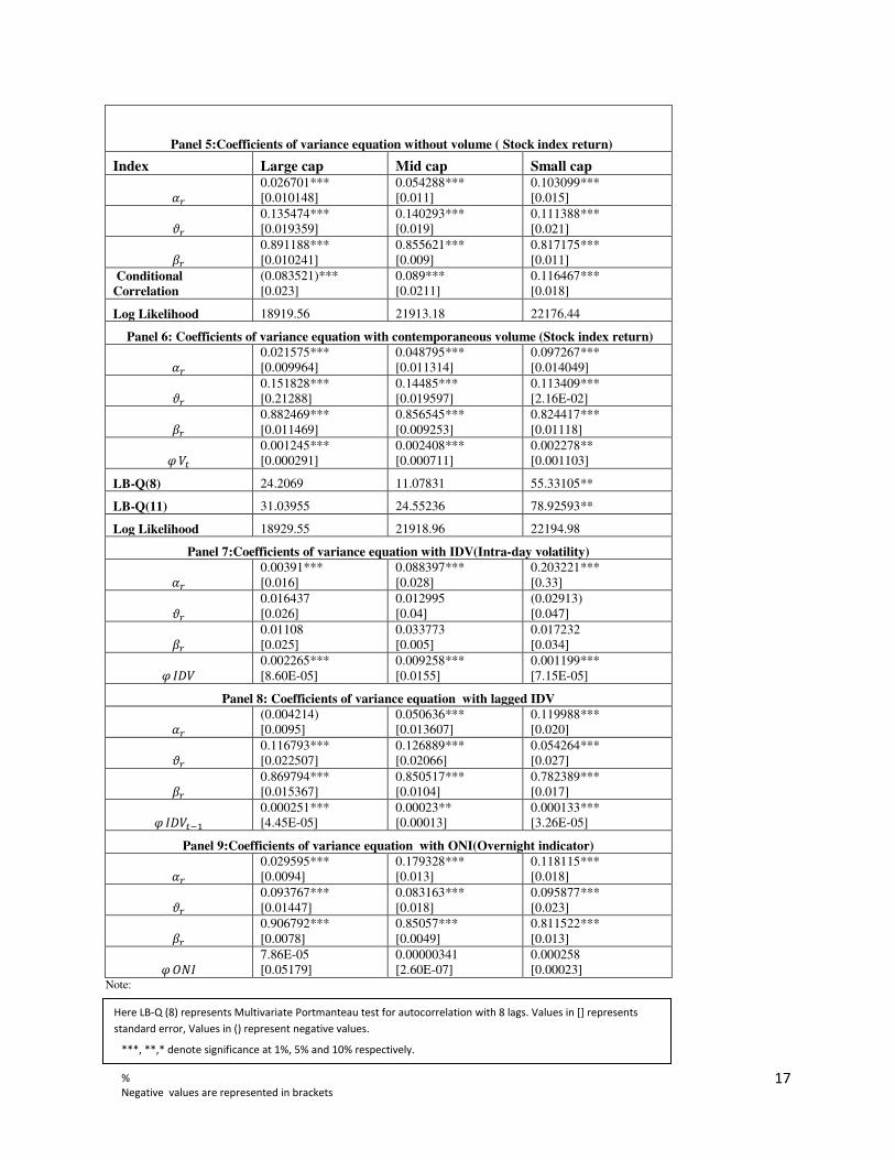
Table 3 gives the model estimates of bivariate GJR–GARCH. It is found that, in the conditional
variance equation of volume, the asymmetric term is significant in all the three indices
considered. Effect of both contemporaneous volume and lagged volume is considered. In
volatility equation of volume, both ARCH and GARCH terms are found to be significant for all
the three indices. It is observed that the persistence in volatility decreases with the decrease
market capitalization. In the conditional variance equation of return of the indices, the
asymmetric term is significant for all the three indices. The persistence in volatility of index
return is measured by 𝛼𝑟 + 𝛽𝑟 + 𝜗𝑟/2 from equation 15. The persistence in volatility is decreasing
with decrease in market capitalization. From Table 3 panel 5, it is observed that in case of all
three indices considered, the coefficient of asymmetric term and innovation terms are significant
that means, direction and magnitude of news both are important in estimating conditional
volatility but, we can say that, direction of news is more important than the magnitude of news as
coefficient of asymmetric term is much larger than lagged innovation term in all the three indices
considered. Table 4 gives the volatility persistence of return. It is evident that there is marginal
decrease in volatility persistence by including volume term in variance equation of the Sensex
and mid-cap indices. For small-cap index, volume does not reduce the volatility persistence.
Gallio and Paccini(2000) discuss ONI and IDV as other measures of information flow. From
Table 3 panel 9, it is evident that ONI is not significant in explaining information flow in
variance equation for large-cap, mid-cap and small-cap indices, whereas IDV is found to be
significant in explaining information flow. Inclusion of IDV in the variance equation makes the
GARCH effect insignificant in all the three indices considered. From Table 3 panel 6, it is

21
evident that both past innovations in return series and lags of volatility of all the three indices are
significant in explaining the current volatility. Inclusion of volume in variance equation is found
to be significant in all the three indices indicating that volume traded explains volatility of return.
Both contemporaneous and lagged volume coefficients are found to be significant in volatility
equation of return of all the three indices. From Table 3 panel 5, it is found that correlation
coefficient between volume and return is significant, and there exist negative correlation between
volume and stock return in Sensex whereas positive correlation between volume and stock return
is found in case of mid-cap and small-cap indices.
5.1 Conditional correlations between volatility and volume traded
To further study the correlation between volatility and volume traded, the volatility of returns of
all the indices is estimated without considering volume as exogenous factor in equation 14. The
restrictive bivariate GJR-GARCH model is used to estimate volatility and volume traded.
From Table 6, it is evident that there exists positive conditional correlation between volatility of
stock return and volume traded in case of Sensex index which is consistent with the past studies.
Conditional correlation between volatility of stock return and volume traded is negative in case
of mid cap index and small cap index. Therefore, it can be inferred that, in case of Sensex as the
volatility increases volume traded also increases. This confirms Tauchen and Pitts(1983)
findings, “in markets where number of trades is large the relation between trading volume and
return volatility should be positive”. In case of small cap and mid cap indices, as the volatility of
index returns increases volume traded decreases. This explains that informed traders tend to lead
the speculative trading activity and drive bid-ask spreads higher, further diminishing the liquidity
of these markets. The negative relation between volume and volatility suggests that both
volatility and trading volume are determined by new information flow to the market, traders
respond to new information arrival and the number of active trades. As a result in thinly traded
and highly volatile markets, infrequent trading can cause prices to deviate substantially from
fundamentals. (see Girard &Biswas (2007) and Tauchin and Pitts (1983)). The negative relation
between volume and volatility is supported by Sequential information hypothesis of
Copeland(1976). In emerging markets dissemination of information is asymmetric and initially
only well informed traders take position. As information is sequentially transmitted from trader
to trader less informed traders also take position. After a series of intermediate transient

22
equilibrium, a final equilibrium is reached resulting in lower volatility. Therefore we find that,
effect of volatility on volume traded is different across different market indices according to
market capitalization.
Table 6
Conditional correlation and Granger causality test between volume and volatility
Index Large- cap Mid- cap Small-cap
Conditional Correlation
0.073675**
[0.029]
(0.027516)*
[0.030]
(0.091138)***
[0.028]
Volume does not Granger causes
variance 128.3247*** 17.95312* 35.50156***
Variance does not Granger causes
volume 22.28712** 22.27961** 29.17906** Note:
5.2 Volume traded information transmission among large-cap, mid-cap and small-cap
indices.
To test the dynamic relation between volumes traded of the three indices, tri-variate restrictive
Vector autoregressive methodology (VAR) is used to study the mean spillover of surprises of
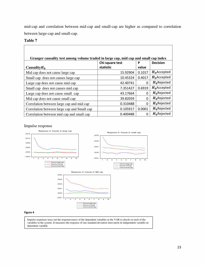
volume traded among the three indices considered on the basis of market capitalization. From
Table 7,it is evident that lags of volume traded of mid cap and small cap does not Granger cause
volume traded in large-cap(Sensex). Whereas, volume traded of large cap Granger causes
volume in mid cap. Lags of volume traded in large cap and small cap Granger causes volume in
small cap index. The mean volume traded in large cap index affects mean volume traded of mid
cap and small cap. Therefore, it can be inferred that, information asymmetry does exist in the
market. New information is first reflected in large cap and then it transmits lo lower indices. To
study the response period and sign of causality Impulse response methodology is used. From fig
4, it can be observed that response of volume of large cap to volume of large cap is high and it is
persistent after 10 lags also. Response of large-cap to mid-cap and small-cap is zero. Mean
response of mid-cap to large-cap is positive that means, if volume traded is high in large-cap that
causes increase in volume traded of mid-cap and vice-versa. Response of small-cap to large-cap
is small but, response of small-cap to mid-cap is quite high and positive. From Table 7, it is
observed that correlation between volume traded of large cap and mid-cap, large-cap and small-
cap and mid-cap and small-cap are positive and significant. Correlation between large cap and
Values in [] represents standard error, Values in () represent negative values.
***,**,* denote significance at 1%,5% and 10% respectively.
In Granger causality test chi-square test statistic value is given.
23
mid-cap and correlation between mid-cap and small-cap are higher as compared to correlation
between large-cap and small-cap.
Table 7
Granger causality test among volume traded in large cap, mid cap and small cap index
Causality𝑯𝟎
Chi square test
statistic
P
value
Decision
Mid cap does not cause large cap 15.92904 0.1017 𝑯𝟎Accepted
Small cap does not causes large cap 10.45324 0.4017 𝑯𝟎Accepted
Large cap does not cause mid cap 42.40741 0 𝑯𝟎Rejected
Small cap does not causes mid cap 7.351427 0.6919 𝑯𝟎Accepted
Large cap does not cause small cap 43.17664 0 𝑯𝟎Rejected
Mid cap does not cause small cap 39.82059 0 𝑯𝟎Rejected
Correlation between large cap and mid cap 0.310488 0 𝑯𝟎Rejected
Correlation between large cap and Small cap 0.105917 0.0001 𝑯𝟎Rejected
Correlation between mid cap and small cap 0.400488 0 𝑯𝟎Rejected
Impulse response
Figure 4
6. Conclusion
-.0004
.0000
.0004
.0008
.0012
.0016
1 2 3 4 5 6 7 8 9 10
Volume large cap
Volume mid cap
Volume small cap
Response of Volume of large cap
-.0001
.0000
.0001
.0002
.0003
.0004
1 2 3 4 5 6 7 8 9 10
Volume large cap
Volume mid cap
Volume small cap
Response of Volume of Mid cap
-.0001
.0000
.0001
.0002
.0003
1 2 3 4 5 6 7 8 9 10
Volume large cap
Volume mid cap
Volume small cap
Response of Volume of small cap
Impulse responses trace out the responsiveness of the dependent variables in the VAR to shocks to each of the
variables in the system. It measures the response of one standard deviation innovation in independent variable on
dependent variable.
24
6. Conclusion
The study investigates relationships among return, trading volume and return volatility of three
different market capitalized indices and effect of information flow on volatility persistence.
Bivariate VAR for mean equations and bivariate GJR-GARCH methodology for the variance
equation are used to study joint dynamics of volume, return and volatility in financial markets.
Three indices of different market capitalization have been considered where, S&P BSE Sensex
represents large capitalization firms, BSE mid-cap represents mid-capitalization firms and BSE
small-cap index represents small capitalization firms. The study investigates the relationship
between return, volume, volatility and the spillover of mean trading activity among indices. The
study considers volume, IDV and ONI as proxy variables for information dissemination in
financial markets. The findings suggest that their exist dynamic and contemporaneous relation
between return of index and volume, in all the three indices considered since lags of index return
causes volume which confirms the findings of Chordia, Huh, and Subrahmanyam (2006),
Gallant, Rossi, and Tauchen (1992) despite using a different methodology, bivariate GARCH. It
is observed that, there exist negative correlation between volume and return of Sensex when
volume and return is used in bivariate specification. In case of mid cap and small cap indices the
correlation between volume and return is found to be positive. It is observed that the persistence
in volatility decreases with the decrease in market capitalization. Bidirectional causality is
observed in case of volume and volatility for all the indices considered. In case of large cap there
is positive conditional correlation between volume and volatility, whereas in case of mid cap and
small cap the correlation coefficient is negative. Correlation between volume and volatility is
strongest in case of small cap. Therefore, it can be inferred that in case of Sensex, as the
volatility increases volume traded also increases. This behavior of Sensex confirms the positive
relation between trading volume and return volatility when the number of traders is large. In the
cases of mid- cap and small-cap indices, volume traded decreases with the increase in volatility
of the indices returns. In case of mid cap and small cap this behavior is in tandem with the
argument, “informed traders tend to lead the speculative trading activity and drive bid-ask
spreads higher, further diminishing the liquidity of the markets”. This shows that the effect of
volatility on volume traded is not similar for three market indices with different market
capitalization. It is evident that the direction of news is more important than the magnitude of
news since the coefficient of asymmetric term in the model is much larger than lagged

25
innovation term coefficient. There is marginal decrease in volatility persistence by including
volume in the variance equation of the Sensex returns. The volume does not have any impact on
the small cap index in decreasing volatility persistence. Both contemporaneous and lagged
volume coefficients are found to be significant in volatility equation of return series of all the
three indices considered. When IDV (Intraday volatility) is taken as a measure of information
arrival, the GARCH effect vanished completely in all the three indices considered. These results
suggest that lagged squared residuals contribute little if any additional information about the
variance of the stock return process is accounted in the model, when the rate of information flow
is measured in terms of contemporaneous IDV. The rate of information arrival measured by IDV
is found to be a significant source of the conditional heteroskedasticity in Indian markets since
the presence of IDV, as a proxy for information flow, makes GARCH term insignificant. The
mean volume traded in large cap index affects the mean volume traded of mid-cap and small-cap
indices. This confirms that the information asymmetry does exist in the market. New information
is first reflected in large cap and then it transmits to lower indices. Hence, volume traded and
volatility of large cap index can be used to model or predict volatility and volume in case of mid
cap and small cap indices. Mean impulse response of mid-cap to large-cap is positive, therefore,
increase in volume traded in large-cap causes increase in volume traded of mid-cap and vice-
versa. Bivariate conditional correlations among volume traded of large-cap, mid-cap and small-
cap are positive and significant. Conditional correlation of volume traded between large-cap and
mid-cap is higher as compared to large-cap and small-cap. This confirms there is information
asymmetry in markets.
References
Admati, A. R. (1988). A theory of intraday patterns: Volume and price variability. Review of
Financial studies , 1(1), 3-40.
Bohl, M. T. (2003). Trading volume and stock market volatility. The Polish case. International
Review of Financial Analysis , 12(5), 513-525.
Bollerslev, T. E. (1988). A capital asset pricing model with time-varying covariances. The
Journal of Political Economy , 116-131.
Bollerslev, T. (1990). Modelling the coherence in short-run nominal exchange rates: a
multivariate generalized ARCH model. The Review of Economics and Statistics , 498-
505.

26
Bollerslev, T. (1990). Modelling the coherence in short-run nominal exchange rates: a
multivariate generalized ARCH model. The Review of Economics and Statistics , 498-
505.
Bollerslev, T., & Wooldridge, J. (1992). Quasi-maximum likelihood estimation and inference in
dynamic models with time-varying covariances. Econometric reviews , 11(2), 143-172.
Campbell, J., Grossman, S., & Wang, J. (1993). Trading volume and serial correlation in stock
returns. Quarterly Journal of Economics , 905–939.
Chen, G. M., Firth, M., & Rui, O. M. (2001). The dynamic relation between stock returns,
trading volume, and volatility. Financial Review , 36(3), 153-174.
Chen, J., Hong, H., & Stein, J. C. (2001). Forecasting crashes: Trading volume, past returns, and
conditional skewness in stock prices. Journal of Financial Economics , 61(3), 345-381.
Chordia, T., & Swaminathan, B. (2000). Trading volume and cross‐autocorrelations in stock
returns. The Journal of Finance , 55(2), 913-935.
Chordia, T., Huh, S., & Subrahmanyam, A. (2007). The cross-section of expected trading
activity. Review of Financial Studies , 709–740.
Chuang, W. I., Liu, H. H., & Susmel, R. (2012). The bivariate GARCH approach to investigating
the relation between stock returns, trading volume, and return volatility. Global Finance
Journal , 23(1), 1-15.
Clark, P. (1973). A Subordinate Stochastic Process Model with Finite Variance for Speculative
Prices. Econometrica , 41 (1) (1973), 135-155.
Clark, P. K. (1973). A subordinated stochastic process model with finite variance for speculative
prices. Econometrica: Journal of the Econometric Society , 135-155.
Copeland, T. (1976). A model of asset trading under the assumption of sequential information
arrival. Journal of Finance , 1149–1168.
Crouch, R. L. (1970). The volume of transactions and price changes on the New York Stock
Exchange. Financial Analysts Journal , 104-109.
Engle, R. F., & Ng, V. K. (1993). Measuring and testing the impact of news on volatility. The
Journal of finance , 48(5), 1749-1778.
Epps, T. W., & Epps, M. L. (1976). The stochastic dependence of security price changes and
transaction volumes: Implications for the mixture-of-distributions hypothesis.
Econometrica: Journal of the Econometric Society , 305-321.
Fama, E. F. (1965). The behavior of stock-market prices. Journal of business , 34-105.

27
Gallant, A. R., Rossi, P. E., & Tauchen, G. (1992). Stock prices and volume. Review of Financial
studies , 5(2), 199-242.
Gallo, G., & Pacini, B. (2000). The effects of trading activity on market volatility. The
European Journal of Finance , 6(2), 163-175.
Gervais, S., Kaniel, R., & Mingelgrin, D. H. (2001). The high‐volume return premium. The
Journal of Finance , 56(3), 877-919.
Girard, E., & Biswas, R. (2007). Trading volume and market volatility: developed versus
emerging stock markets. Financial Review , 42(3), 429-459.
Granger, C. W., & Morgenstern, O. (1963). Spectral analysis of New york stock market pricess.
Kyklos , 16(1), 1-27.
Harris, M., & Raviv, A. (1993). Differences of opinion make a horse race. Review of Financial
studies , 6(3), 473-506.
He, H., & Wang, J. (1995). Differential informational and dynamic behavior of stock trading
volume. Review of Financial Studies , 8(4), 919-972.
Hiemsta, D., & Jones, J. (1994). Testing for Linear and Nonlinear Granger Causality in the Stock
Price‐Volume Relation. The Journal of Finance , 49(5), 1639-1664.
Jain, P. C., & Joh, G. H. (1988). The dependence between hourly prices and trading volume.
Journal of Financial and Quantitative Analysis , 23(03), 269-283.
Jennings, R. H., Starks, L. T., & Fellingham, J. C. (1981). An equilibrium model of asset trading
with sequential information arrival. The Journal of Finance , 36(1), 143-161.
Karpoff, J. M. (1986). A theory of trading volume. The Journal of Finance , 41(5), 1069-1087.
Kim, D., & Kon, S. J. (1994). Alternative models for the conditional heteroscedasticity of stock
returns. Journal of Business , 563-598.
Lamoureux, C. G., & Lastrapes, W. D. (1994). Endogenous trading volume and momentum in
stock-return volatility. Journal of Business & Economic Statistics , 12(2), 253-260.
Lamoureux, C. G., & Lastrapes, W. D. (1990). Persistence in variance, structural change, and the
GARCH model. Journal of Business & Economic Statistics , 8(2), 225-234.
Lee, B. S., & Rui, O. M. (2002). The dynamic relationship between stock returns and trading
volume: Domestic and cross-country evidence. Journal of Banking & Finance , 26(1),
51-78.
28
Lo, A. W., & Wang, J. (2000). Trading volume: definitions, data analysis, and implications of
portfolio theory. Review of Financial Studies , 13(2), 257-300.
Lucey, B. M. (2005). Does volume provide information? Evidence from the Irish stock market.
Applied Financial Economics Letters , 1(2), 105-109.
Omran, M. F., & McKenzie, E. (2000). Heteroscedasticity in stock returns data revisited: volume
versus GARCH effects. Applied Financial Economics , 10.5 (2000): 553-560.
Osborne, M. F. (1959). Brownian motion in the stock market. Operations research , 7(2), 145-
173.
Pagan, A. (1984). Econometric issues in the analysis of regressions with generated regressors.
International Economic Review , 221-247.
Poon, S. H., & Granger, C. W. (2003). Forecasting volatility in financial markets: A review.
Journal of economic literature , 41(2), 478-539.
Pyun, C. S., Lee, S. Y., & Nam, K. (2001). Volatility and information flows in emerging equity
market: A case of the Korean stock exchange. International Review of Financial
Analysis , 9(4), 405-420.
Ranter, M., & Leal, R. (2001). Stock returns and trading volume: Evidence from the emerging
markets of Latin America and Asia. Journal of Emerging Markets , 6, 5–22.
Rogalski, R. J. (1978). The dependence of prices and volume. The Review of Economics and
Statistics , 268-274.
Rozga, A., & Arneric, J. (2009). dependence between volatility persistence, kurtosis and degree
of freedom. Investigación Operacional , 30(1), 32-39.
Silvapulle, P., & Choi, J. S. (1999). Testing for linear and nonlinear Granger causality in the
stock price-volume relation: Korean evidence. The Quarterly Review of Economics and
Finance , 39(1), 59-76.
Tauchen, G. E., & Pitts, M. (1983). The price variability-volume relationship on speculative
markets. Econometrica: Journal of the Econometric Society , 485-505.
Westerfield, R. (1977). The distribution of common stock price changes: An application of
transactions time and subordinated stochastic models. Journal of Financial and
Quantitative Analysis , 12(05), 743-765.
Top Related