


Languages
Pages
Legal


Information and Entanglement Measures
in Quantum Systems
with Applications to Atomic Physics
TESIS DOCTORAL
por
Daniel Manzano Diosdado
Departamento de Fısica Atomica, Molecular y Nuclear
Universidad de Granada
Marzo, 2010

Editor: Editorial de la Universidad de GranadaAutor: Daniel Manzano DiosdadoD.L.: GR 3094-2010ISBN: 978-84-693-3310-5


A Raquel

Tesis doctoral dirigida por:
Dr. Jesus Sanchez-Dehesa
Dr. Angel Ricardo Plastino


D. Jesus Sanchez-Dehesa Moreno-Cid, Doctor en Fısica, Doctor en Matematicas y Cat-
edratico del Departamento de Fısica Atomica, Molecular y Nuclear de la Facultad de
Ciencias de la Universidad de Granada, y
D. Angel Ricardo Plastino, Doctor en Astronomıa e Investigador de Reconocida Valıa
de la Junta de Andalucıa del Departamento de Fısica Atomica, Molecular y Nuclear de
la Facultad de Ciencias de la Universidad de Granada.
MANIFIESTAN:
Que la presente Memoria titulada “Information and Entanglement Measures in Quan-
tum Systems with Applications to Atomic Physics”, presentada por Daniel Manzano
Diosdado para optar al Grado de Doctor en Fısica, ha sido realizada bajo nuestra di-
reccion en el Departamento de Fısica Atomica, Molecular y Nuclear de la Universidad
de Granada y el Instituto Carlos I de Fısica Teorica y Computacional de la Universidad
de Granada.
Granada, 3 de Marzo de 2010
Fdo.: Jesus Sanchez-Dehesa Moreno-Cid.
Fdo.: Angel Ricardo Plastino.
Memoria presentada por Daniel Manzano Diosdado para optar al Grado de Doctor en
Fısica por la Universidad de Granada.
Fdo.: Daniel Manzano Diosdado.


Tıtulo de Doctor con Mencion Europea
Con el fin de obtener la Mencion Europea en el Tıtulo de Doctor, se han cumplido, en
lo que atane a esta Tesis Doctoral y a su Defensa, los siguientes requisitos:
1. La tesis esta redactada en ingles con una introduccion en espanol.
2. Dos de los miembros del tribunal provienen de una universidad europea no espanola.
3. Una parte de la defensa se ha realizado en ingles.
4. Una parte de esta Tesis Doctoral se ha realizado en Austria, en el Instituto de
Optica e Informacion Cuantica de Viena.


Agradecimientos
Primero quisiera agradecer a mis directores de tesis el haber hecho posible la realizacion
de esta tesis. A Jesus por depositar su confianza en mi cuando era aun un estudiante
y por darme una oportunidad que mis resultados academicos me negaban. A Angel
por dedicar pacientemente tanto tiempo a explicarme esos conceptos que continuamente
se me escapan. En definitiva ambos me han dado la oportunidad de formarme como
cientıfico.
Al Instituto de Optica Cuantica e Informacion Cuantica de Viena, y todos mis companeros
de allı por haberme acogido durante mis estancias, por haberme ensenado tanto y por
abrirme tantas puertas.
A mis companeros fısicos. Jorge, Alex, Antonio, Jesus, Pablo, Paki, Belen y Lidia (que
no es fısica pero poco le falta), por aguantarme durante y despues de la carrera, por
tantas tardes de estudio y noches de celebracion del fin de examenes, por disenar teorıas
tan originales y rigurosas como el perrato y el elefantache. A Sheila y a Bea por todo
eso y por hacerme tan agradable el ir al despacho a trabajar, tambien por dejarse ganar
siempre al mus para levantarme la autoestima.
A mis amigos de Algeciras. Pablo, Sergio, Gabi, Juanlu, Alvaro y Eva. Por estar ahı
desde hace tanto tiempo y proveerme de tantas anecdotas para contar que ya parezco
un viejo.
A mis amigos del club Treparriscos, en especial a Yamil, Joaquın y Lore. Por tantas
tardes en el rocodromo del club y Armilla, tantas vıas escaladas y montanas subidas,
tantas cervezas tomadas despues y por ensenarnos mutuamente que el esfuerzo tiene
siempre recompensa.
A mis abuelos, tıos, tıas, primos, primas, cunadas, cunados, suegra, suegro y sobrino,
que son demasiados para nombrarlos a todos. Porque aunque no nos vemos tanto como
quisieramos tengo la suerte de formar parte de una familia estupenda por todos los lados.
A mis padres por haberme animado siempre a ser yo mismo, por regalarme libros de
ciencia y muchos otros temas, por animarme tanto durante la carrera y apoyar siempre
mis decisiones. En definitiva porque de no ser por ellos esta tesis sin duda nunca se
habrıa escrito.
A mi hermano. Por ser mi companero de piso tantos anos y que nos llevaramos ra-
zonablemente bien. Por escucharme con atencion siempre que le cuento algo de fısica
y explicarme con paciencia las cosas cuando me adentro en otras cuestiones. Por esos
anos juntos en el balonmano que tanto nos unieron y los posteriores en la montana que
lo estan haciendo aun mas. En general por ejercer su rol de hermano mayor.
A Leonard Hofstadter, Howard Wolowitz, Rajesh Koothrappali y Sheldon Cooper por
hacer mundialmente conocido que la fısica puede ser muy divertida. Bazinga!
Y por supuesto a Raquel por todo lo anterior y mucho mas.

Contents
Foreword I
Introduccion III
Author’s publications VII
1 Configuration complexities of hydrogenic atoms 3
1.1 The hydrogenic problem: Information-theoretic measures . . . . . . . . . 5
1.2 Composite information-theoretic measures of hydrogenic orbitals . . . . . 9
1.3 Upper bounds to the Fisher-Shannon measure and shape complexity . . . 15
1.4 Conclusions . . . . . . . . . . . . . . . . . . . . . . . . . . . . . . . . . . . 17
2 Complexity of D-dimensional hydrogenic systems in position and mo-mentum spaces 19
2.1 The D-dimensional hydrogenic quantum-mechanical densities . . . . . . . 21
2.2 The LMC shape complexity of the D-dimensional hydrogenic system . . . 22
2.2.1 Position space . . . . . . . . . . . . . . . . . . . . . . . . . . . . . . 22
2.2.2 Momentum space . . . . . . . . . . . . . . . . . . . . . . . . . . . . 24
2.3 LMC shape complexities of ground and circular states . . . . . . . . . . . 25
2.3.1 Ground state . . . . . . . . . . . . . . . . . . . . . . . . . . . . . . 25
2.3.2 Circular states . . . . . . . . . . . . . . . . . . . . . . . . . . . . . 27
2.4 Numerical study and physical discussion . . . . . . . . . . . . . . . . . . . 28
2.5 Conclusions . . . . . . . . . . . . . . . . . . . . . . . . . . . . . . . . . . . 32
3 Entropy and complexity analyses of Klein-Gordon systems 33
3.1 Klein-Gordon equation for Coulomb systems: Basics . . . . . . . . . . . . 35
3.2 Relativistic charge effects by information measures . . . . . . . . . . . . . 37
3.2.1 Radial expectation values and Heisenberg’s measure. . . . . . . . . 38
3.2.2 Shannon and Fisher information measures . . . . . . . . . . . . . . 41
3.3 Complexity analysis of Klein-Gordon single-particle systems . . . . . . . . 45
3.3.1 The Fisher-Shannon measure of pionic systems . . . . . . . . . . . 46
3.3.2 The LMC shape complexity of pionic systems . . . . . . . . . . . . 48
3.4 Conclusions . . . . . . . . . . . . . . . . . . . . . . . . . . . . . . . . . . . 50
4 Information-theoretic lengths of orthogonal polynomials 51
4.1 Spreading lengths of classical orthogonal polynomials . . . . . . . . . . . . 52
4.2 Spreading lengths of Hermite polynomials . . . . . . . . . . . . . . . . . . 55
4.2.1 Ordinary moments and the standard deviation . . . . . . . . . . . 55
XIII

XIV CONTENTS
4.2.2 Entropic moments and Renyi lengths of integer order q . . . . . . 56
4.2.3 Shannon length: Asymptotics and sharp bounds . . . . . . . . . . 58
4.2.4 Fisher length . . . . . . . . . . . . . . . . . . . . . . . . . . . . . . 60
4.2.5 Effective computation of the spreading lengths . . . . . . . . . . . 60
4.2.6 Application . . . . . . . . . . . . . . . . . . . . . . . . . . . . . . . 62
4.2.7 Open problems . . . . . . . . . . . . . . . . . . . . . . . . . . . . . 64
4.3 Direct spreading measures of Laguerre polynomials . . . . . . . . . . . . . 66
4.3.1 Ordinary moments, standard deviation and Fisher length . . . . . 68
4.3.2 Renyi lengths . . . . . . . . . . . . . . . . . . . . . . . . . . . . . . 69
4.3.2.1 Algebraic approach . . . . . . . . . . . . . . . . . . . . . 70
4.3.2.2 Combinatorial approach . . . . . . . . . . . . . . . . . . . 71
4.3.3 Shannon length: Asymptotics and sharp bounds . . . . . . . . . . 73
4.3.4 Some computational issues . . . . . . . . . . . . . . . . . . . . . . 75
4.4 Conclusions . . . . . . . . . . . . . . . . . . . . . . . . . . . . . . . . . . . 79
5 Quantum learning 81
5.1 The speed of quantum and classical learning . . . . . . . . . . . . . . . . . 82
5.2 Conclusions . . . . . . . . . . . . . . . . . . . . . . . . . . . . . . . . . . . 88
6 Quantum Entanglement 91
6.1 Composite systems with distinguishable subsystems . . . . . . . . . . . . 93
6.2 Systems of identical fermions . . . . . . . . . . . . . . . . . . . . . . . . . 95
7 Identical fermions, entanglement and two-electron systems 101
7.1 Separability criteria and entanglement measures for pure states of N iden-tical fermions . . . . . . . . . . . . . . . . . . . . . . . . . . . . . . . . . . 102
7.1.1 Separability criteria . . . . . . . . . . . . . . . . . . . . . . . . . . 103
7.1.2 Entanglement measures . . . . . . . . . . . . . . . . . . . . . . . . 109
7.2 Quantum entanglement in two-electron atomic models . . . . . . . . . . . 112
7.2.1 Quantum entanglement in systems of two identical fermions . . . . 113
7.2.2 The Crandall and Hooke atoms . . . . . . . . . . . . . . . . . . . . 115
7.2.3 Entanglement in the Crandall atom . . . . . . . . . . . . . . . . . 118
7.2.4 Entanglement in the Hooke atom . . . . . . . . . . . . . . . . . . . 121
7.2.5 Entanglement in helium-like atoms . . . . . . . . . . . . . . . . . . 121
7.3 Separability criteria for continuous quantum systems . . . . . . . . . . . . 124
7.3.1 Description of the criteria . . . . . . . . . . . . . . . . . . . . . . . 125
7.3.2 Analysis for pure states . . . . . . . . . . . . . . . . . . . . . . . . 130
7.3.3 Analysis for mixed states . . . . . . . . . . . . . . . . . . . . . . . 136
7.4 Conclusions . . . . . . . . . . . . . . . . . . . . . . . . . . . . . . . . . . . 142
Apendix A. Radial and angular contributions to the hydrogenic disequi-librium 143
Apendix B. pth-power of a polynomial of degree n and Bell polynomials147
Apendix C. Information and complexity measures 148
Bibliography 155

Foreword
This thesis is a multidisciplinary contribution to the information theory of single-particle
Coulomb systems (see Chapters 1, 2 and 3), to the theory of special functions of math-
ematical physics (Chapter 4), to quantum computation (Chapter 5) and to quantum
information and atomic physics (Chapters 6 and 7). The notions of information, com-
plexity and entanglement play a central role.
The Chapters are self-contained with their own Introduction and Conclusions. They
may be read in arbitrary order and correspond to one (Chapters 1, 2 and 5) or two
(Chapters 3, 4 and 7) scientific publications.
In Chapter 1 we explore both analytically and numerically the internal disorder of the
hydrogenic atom which is associated to the non-uniformity of the quantum-mechanical
probability density of its physical states, and which gives rise to the great diversity of
three-dimensional geometries of its configuration orbitals. This is done for the ground
and excited stationary states not only with the variance and the disequilibrium, but
also by means of the Fisher-Shannon, Cramer-Rao and LMC shape complexities in po-
sition and momentum spaces. The dependence of these composite information-theoretic
measures on the nuclear charge Z and the three quantum numbers (n, l, m) of the
orbitals is carefully examined. Briefly, it is found that the three complexity measures
do not depend on Z and that the Fisher-Shannon measure quadratically depends on n.
Moreover, the explicit expression of the shape complexity is obtained and sharp bounds
to the Fisher-Shannon measure are given.
Chapter 2 generalizes to D dimensions some of the themes from the preceding chapter.
In it we provide the mathematical description of a formalism to calculate the LMC
shape complexity of arbitrary stationary states of the D-dimensional hydrogenic system
in terms of certain entropic functionals of the Laguerre and Gegenbauer or ultrashperical
polynomials. We emphasize the ground and circular states, where the shape complexity
is explicitly calculated and discussed in terms of the dimensionality and the quantum
numbers. Then, the dimensional and Rydberg energy limits as well as their associated
uncertainty products are explicitly given.
In Chapter 3 we extend the work done in the two previous chapters to include the rela-
tivistic effects at the Klein-Gordon level. Precisely, we investigate the relativistic charge
I

II Foreword
compression of spinless Coulomb particles by means of various single (variance, Shannon
entropy and Fisher information) and composite (Fisher-Shannon and LMC shape com-
plexity) information-theoretic measures both qualitative and quantitatively. The three
single charge spreading measures show that the relativistic effects are bigger (i.e. the
charge compresses more towards the origin) for the low-lying energetic states and when
the nuclear charge increases. Moreover, the relativistic effects enhance the variance and
the Shannon information when n (l) decreases for fixed l (n); the Fisher information has
the opposite behaviour. Moreover, the Fisher-Shannon complexity increases with the
magnetic quantum number for fixed (n, l). It is observed, once the Lorentz invariance
is appropriately taken into account, that the Shannon-Fisher and LMC complexities
increases with the nuclear charge, contrary to the non-relativistic case.
In Chapter 4 we introduce the direct spreading measures of a family of special func-
tions of the mathematical physics, the orthogonal hypergeometric polynomials, which
quantify the spread of their associated Rakhmanov probability density all over their
orthogonality interval in various complementary ways. Then, we emphasize the Hermite
and Laguerre polynomials where we calculate not only the ordinary moments and stan-
dard deviation, but also the information-theoretic lengths of Renyi, Shannon and Fisher
types. This is done for the Renyi measure by the use of a general methodology which
uses the multivariable Bell polynomials so useful in Combinatorics and, in the Laguerre
case, the linearization technique of Srivastava and Niukkanen. For the Shannon length,
which cannot be analytically calculated because of its logarithmic functional form, its
asymptotics and some upper bounds are obtained. The Fisher length is explicitly given.
Later on, all the direct spreading measures of these polynomials are mutually compared
and computationally analyzed.
Chapter 5 is a contribution in the field of learning processes for quantum computers that
realizes classical operations. We propose a new model for making a quantum automaton
for the processing of classical information. It is based in a machine that can make any
unitary operation in one qubit. The operation used for testing the learning procedure is
the kth root of NOT (logical negation) of a bit, that is a well defined classical operation.
It is proved that the learning time for the quantum machine is independent of the root of
the operation, but for any classical machine it will scale quadratically with k for k = 2m,
being m a natural number. Finally the speed of both a classical learning model and the
quantum learning model is compared.
In Chapter 6 the state of the art in the field of entanglement and its applications to
fermionic systems is reviewed. Special emphasis is done on separability criteria and en-
tanglement measures for systems with distinguishable and indistinguishable subsystems
and in the definition of entanglement for identical fermionic systems.
In Chapter 7, attention turns to the study of the entanglement properties of multi-
fermionic systems. First, based on the linear and von Neumann entropies of the single

Foreword III
particle reduced density matrix, we found separability criteria for pure states of N identi-
cal fermions which are much simpler than the criteria recently proposed in the literature.
Then we derive some inequalities for these entropies which allow us to propose natu-
ral entanglement measures for N -fermion pure states. Moreover, they connection with
classical Hartree-Fock results are pointed out. After that, the new measures are used
to study the entanglement properties of both ground and excited states of two exactly
solvable systems of two charged fermions and compare them with those of the helium-
like atoms by use of high-quality Kinoshita-like eigenfunctions. The dependence of the
entanglement on the strength of the confining potential has been studied. Briefly, it
is found in all cases that the amount of entanglement tends to grow when the energy
is increasing. The dependence of the entanglement on the parameter of the models as
well as on the nuclear charge is also investigated. Finally, a new criterion proposed by
Walborn et al [1] in 2009 for the detection of entanglement in quantum systems with
continuous variables is numerically analyzed.


Introduccion
Esta tesis es una contribucion multidisciplinar a la teorıa de la informacion de sistemas
monoparticulares Coulombianos (ver Capıtulos 1, 2 and 3), a la teorıa de informacion de
las funciones especiales de la fısica matematica (Capıtulo 4), a la computacion cuantica
(Capıtulo 5) y a la informacion cuantica de sistemas atomicos (Capıtulos 6 and 7). Los
conceptos de informacion, complejidad y entrelazamiento juegan un papel principal.
Los Capıtulos son autocontenidos, con su propia introduccion y conclusiones. Cada uno
corresponde a una (Capıtulos 1, 2 y 5) o dos (Capıtulos 3, 4 y 7) publicaciones cientıficas.
En el Capıtulo 1 exploramos analıtica y numericamente el desorden interno del atomo
de hidrogeno, que esta asociado a la no uniformidad de la densidad de probabilidad
mecano-cuantica de sus estados, la cual esta relacionada con la gran diversidad de geo-
metrıas tridimensionales de los orbitales atomicos. Este estudio se realiza para el estado
fundamental y estados excitados no solo mediante la determinacion de la varianza y el
desequilibrio, sino tambien por medio de las complejidades Fisher-Shannon, Cramer-Rao
y LMC, tanto en el espacio de momentos como en el de posiciones. Se examina cuida-
dosamente la dependencia de estas tres medidas con la carga nuclear Z y los numeros
cuanticos (n, l, m). En resumen, se encuentra que estas tres medidas de complejidad
no dependen de Z, y que la medida de Fisher-Shannon depende cuadraticamente de n.
Ademas se dan expresiones explıcitas de la medida LMC ası como cotas precisas a la
medida de Fisher-Shannon.
El Capıtulo 2 generaliza a sistemasD dimensionales algunos de los resultados del capıtulo
anterior. En el se describe un formalismo fisico-matematico de calculo de la complejidad
LMC de estados estacionarios arbitrarios de un sistema hidrogenoide D-dimensional en
terminos de ciertos funcionales entropicos de los polinomios de Laguerre y Gegenbauer
o ultraesfericos. Se hace hincapie en el estado fundamental y los estados circulares,
donde la complejidad LMC se calcula explıcitamente y es analizada en funcion de la
dimensionalidad y de los numeros cuanticos.
El Capıtulo 3 extiende el trabajo hecho en los dos capıtulos anteriores para incluir
los efectos relativistas de tipo Klein-Gordon. Concretamente, investigamos la com-
presion de la carga de partıculas Columbianas sin espın mediante varias medidas teorico-
informacionales de tipo simple (varianza, entropıa de Shannon e informacion de Fisher)
V

VI Introduccion
y compuesto (complejidades Fisher-Shannon y LMC). Las tres medidas simples mues-
tran que los efectos relativistas son mas importantes (i.e. la carga se comprime mas
hacia el origen) para los estados de baja energıa y cuando la carga nuclear aumenta.
Ademas los efectos relativistas aumentan las medidas de dispersion simple (varianza y
entropıa de Shannon) cuando n(l) disminuye para un l(n) fijo, mientras la informacion
de Fisher tiene un comportamiento opuesto. La medida de Fisher-Shannon tambien
aumenta con el numero cuantico magnetico para un (n, l) fijo. Se observa tambien que
las complejidades de Fisher-Shannon y LMC aumentan con el numero atomico Z, al
contrario que en el caso no relativista.
En el Capıtulo 4 introducimos las medidas de esparcimiento directas de una familia de
funciones especiales de la fısica-matematica, los polinomios ortogonales hipergeometricos,
que cuantifican de varias maneras la distribucion de sus densidades de probabilidad de
Rakhmanov en todo su intervalo de ortogonalidad de. Hacemos hincapie en el caso de los
polinomios de Hermite y Laguerre, donde calculamos no solo los momentos ordinarios y la
desviacion estandar, sino tambien las longitudes de las medidas teorico-informacionales
de Renyi, Shannon y Fisher. Esto se realiza para la medida de Renyi mediante el uso de
una metodologıa general que usa los polinomios de Bell multivariables y, en el caso de los
polinomios de Laguerre, mediante la formula de linealizacion de Srivastava y Niukkanen.
Para la longitud de Shannon, que no puede ser calculada analıticamente debido a que
es un funcional logarıtmico, se determinan su asintotica y cotas superiores. La longitud
de Fisher se obtiene explıcitamente. Finalmente, todas estas medidas son comparadas
entre si y analizadas computacionalmente
El Capıtulo 5 es una contribucion al campo de los procesos de aprendizaje para com-
putadores cuanticos que realizan operaciones clasicas. Proponemos un nuevo modelo
para realizar un automata cuantico para el procesado de informacion clasica. Este se
basa en una maquina que puede realizar una operacion arbitraria en un qubit. La ope-
racion usada para testear el proceso de aprendizaje es la raız k-esima de la operacion
NOT (negacion logica) de un bit, que es una operacion clasica. Se puede probar que
el tiempo de aprendizaje para la maquina cuantica es independiente de la raız de la
operacion k; por otro lado la maquina clasica escala cuadraticamente con k si k = 2m,
siendo m un numero natural. Finalmente se compara la velocidad de aprendizaje de un
modelo clasico con la del modelo cuantico propuesto.
En el Capıtulo 6 se revisa brevemente el concepto de entrelazamiento cuantico, haciendo
enfasis en las diferencias existentes entre el concepto de entrelazamiento en sistemas
constituidos por subsistemas distinguibles y el correspondiente concepto en sistemas de
fermiones identicos.
En el Capıtulo 7 se investiga el entrelazamiento de sistemas multifermionicos y de vari-
ables continuas. Primero, basandonos en las entropıas lineal y de von Neumann de la
matriz densidad reducida, encontramos criterios de separabilidad para estados puros de

Introduccion VII
N fermiones identicos mucho mas simples que otros criterios recientemente propuestos
en la literatura. Derivamos unas desigualdades para estas entropıas que nos permiten
proponer medidas de entrelazamiento para sistemas puros de N fermiones. Ademas se
analizan las conexiones existentes entre estos resultados y ciertos resultados clasicos de la
teorıa de Hartree-Fock. Estas nuevas medidas se aplican al estudio de las propiedades de
entrelazamiento, tanto para el estado fundamental como para estados excitados, de dos
modelos resolubles de dos fermiones identicos interactuantes, y se comparan los resulta-
dos con un modelo del helio basado en funciones de onda de tipo Kinoshita altamente
precisas. Se explora la dependencia del entrelazamiento con la intensidad del potencial
de confinamiento. Brevemente, se encuentra que en todos estos casos el entrelazamiento
crece al aumentar la energıa. Tambien se estudia la dependencia del entrelazamiento con
los parametros de los modelos, ası como con la carga nuclear. Finalmente se exploran
numericamente diversos aspectos un criterio de separabilidad recientemente propuesto
por Walborn et al [1] para sistemas cuanticos de variables continuas, analizandose su
eficiencia en funcion de diferentes parametros.

Author’s publications
Plastino, A.R., Manzano, D. and Dehesa,J.S. Separability Criteria and Entanglement
Measures for Pure States of N Identical Fermions. EPL (Europhysics Letters) 86 20005
(2009).
Lopez-Rosa, S., Manzano, D. and Dehesa, J.S.. Complexity of D-dimensional hydrogenic
systems in position and momentum spaces. Physica A. 388 (2009) 3273.
J.S. Dehesa, S. Lopez-Rosa, and D. Manzano. Configuration Complexity of Hydrogenic
Atoms. European Physical Journal D. 55 539 (2009).
S. Lopez-Rosa, D. Manzano and J.S. Dehesa. Multidimensional hydrogenic complexities.
Mathematical Physics and Field Theory: Julio Abad, in memoriam. Editors M. Asorey
et al. Zaragoza: Prensas Universitarias de Zaragoza, (2009). See also arXiv:0907.0570.
D. Manzano, M. Paw lowski, C and Brukner. The speed of quantum and classical learning
for performing the k-th root of NOT. New Journal of Physics. 11 113018 (2009).
P. Sanchez-Moreno, J.S. Dehesa, D. Manzano, R.J. and Yanez. Spreading lengths of
Hermite polynomials. Journal of Computational and Applied Mathematics. 233 2136
(2010).
D. Manzano, J.S. Dehesa, and R.J. Yanez. Relativistic Klein-Gordon charge effects by
information-theoretic measures. New Journal of Physics. 12 023014 (2010).
J.S. Dehesa, S. Lopez-Rosa and D. Manzano. Entropy and complexity analyses of D-
dimensional quantum systems. In special issue: “Statistical Complexities: Application
to Electronic Structure”, edited by K.D. Sen. Springer, Berlin, (2010).
D. Manzano, A.R. Plastino, J.S. Dehesa and T. Koga. Quantum entanglement in two-
electron atomic models. J. Phys. A. (2010). Accepted.
D. Manzano, S. Lopez-Rosa and J.S. Dehesa. Complexity analysis of Klein-Gordon
single particle systems. Submitted for publication.
IX
Introduccion 1
P. Sanchez-Moreno, D. Manzano and J.S. Dehesa. Direct spreading measures of Laguerre
polynomials. Submitted for publication.
D. Manzano, A.R. Plastino and J.S. Dehesa. Some features of two entropic separability
criteria for continuous quantum systems. Preprint.

Chapter 1
Configuration complexities of
hydrogenic atoms
A basic problem in information theory of natural systems is the identification of the
proper quantifier(s) of their complexity or internal disorder at their physical states.
Presently this remains open not only for a complicated system, like e.g. a nucleic acid
(either DNA or its single-strand lackey, RNA) in its natural (decidedly non-crystalline)
state, but also for the simplest quantum-mechanical realistic systems, including the
hydrogenic atom. Indeed there does not yet exist any quantity to properly measure
the rich variety of three-dimensional geometries of the hydrogenic orbitals, which are
described by means of three integer numbers: the principal, orbital and magnetic or
azimuthal quantum numbers usually denoted by n, l and m, respectively.
The root-mean-square or standard deviation does not measure the extent to which the
electronic distribution is in fact concentrated, but rather the separation of the region(s)
of concentration from a particular point of the distribution (the centroid or mean value),
so that it is only useful for the nodeless ground state. In general, for excited states (whose
probability densities are strongly oscillating) it is a misleading (and, at times, undefined)
uncertainty measure. To take care of these defects, some information-theoretic quantities
have been proposed: the Shannon entropic power [2, 3] defined by
H [ρ] = exp S [ρ] ; with S [ρ] = −∫ρ (~r) log ρ (~r) d~r, (1.1)
the averaging density or disequilibrium [4–9] defined by
〈ρ〉 =
∫[ρ (~r)]2 d~r, (1.2)
3

4 Chapter 1 Configuration complexities of hydrogenic atoms
and the Fisher information [10] defined by
I [ρ] =
∫ρ (~r)
[~∇ log ρ (~r)
]2d~r. (1.3)
The two former quantities measure differently the total extent or spreading of the elec-
tronic distribution. Moreover, they have a global character because they are quadratic
and logarithmic functionals of the associated probability density ρ (~r). On the contrary,
the Fisher information has a locality property because it is a gradient functional of the
density, so that it measures the pointwise concentration of the electronic cloud and quan-
tifies its gradient content, providing a quantitative estimation of the oscillatory character
of the density. Moreover, the Fisher information measures the bias to particular points
of the space, i.e. it gives a measure of the local disorder.
These three information-theoretic elements, often used as uncertainty measures, have
shown (i) to be closely connected to various fundamental and/or experimentally mea-
surable quantities (e.g., kinetic energy, ionization potential,..) (see e.g. [11, 12]) and
(ii) to exhibit the periodicity of the atomic shell structure (see e.g. [11, 13, 14]). More
recently, various composite information-theoretic measures have been introduced which
have shown not only these properties but also other manifestations of the complexity of
the atomic systems. Let us just mention the Fisher-Shannon measure defined by
CFS [ρ] = I [ρ] × J [ρ] , with J [ρ] =1
2πeexp (2S [ρ] /3) , (1.4)
the Cramer-Rao or Fisher-Heisenberg measure (see e.g. [11, 15, 16]) defined by
CCR [ρ] = I [ρ] × V [ρ] , with V [ρ] =⟨r2⟩− 〈r〉2 , (1.5)
and the LMC shape complexity [6, 17] defined by
CSC [ρ] = 〈ρ〉 ×H [ρ] (1.6)
They quantify different facets of the internal disorder of the system which are manifest
in the diverse and complex three-dimensional geometries of its orbitals. The Fisher-
Shannon measure grasps the oscillatory nature of the electronic probability cloud to-
gether with its total extent in the configuration space. The Cramer-Rao quantity takes
also into account the gradient content but jointly with the electronic spreading around
the centroid. The shape complexity measures the combined effect of the average height
and the total spreading of the probability density; so, being insensitive to the electronic
oscillations. This measure exhibits the important property of scale invariance, which the
original LMC measure [6] lacks, as it was first pointed out by Anteneodo and Plastino
[4].

Chapter 1 Configuration complexities of hydrogenic atoms 5
However, it has not yet been proved its usefulness to disentangle among the rich three-
dimensional atomic geometries of any physical system, not even for the hydrogenic atom
although some properties have been recently found [18]. In this Section we will inves-
tigate this issue by means of the three composite information-theoretic measures just
mentioned for general hydrogenic orbitals in position and momentum spaces. Briefly,
let us advance that here we find that the Fisher-Shannon measure turns out to be the
most appropriate measure to describe the (intuitive) complexity of the three dimensional
geometry of hydrogenic orbitals.
Nevertheless we should immediately say that these three measures are complementary
in the sense that, according to its composition, they grasp different facets of the internal
disorder of the system which are manifest in the great diversity and complexity of con-
figuration shapes of the probability density ρ (~r) corresponding to its orbitals (n, l,m).
The Fisher-Shannon and Cramer-Rao measures have an ingredient of local character
(namely, the Fisher information) and another one of global character (the modified Sha-
nnon entropic power in the Fisher-Shannon case and the variance in the Cramer-Rao
case). The shape complexity is composed by two global ingredients: the disequilibrium
and the Shannon entropic power; so, this quantity is not well prepared to grasp the
oscillating nature of the hydrogenic orbitals but it takes into account the average height
and the total extent of the electron distribution. The Fisher-Shannon measure appro-
priately describes the oscillating nature together with the total extent of the probability
cloud of the orbital. The Cramer-Rao measure takes into account the gradient content
jointly with the spreading of the probability density around its centroid.
The structure of the Chapter is the following. First, in Section 1.1, the hydrogenic
problem is briefly reviewed to fix notations and to gather the known results about the
information-theoretic measures of the hydrogenic orbitals. In Section 1.2, the three
composite measures mentioned above are discussed both numerically and analytically
for the ground and excited hydrogenic states. In Section 1.3, various sharp upper bounds
for these composite measures are provided in terms of the three quantum numbers of
the orbital. Finally, some conclusions are given.
1.1 The hydrogenic problem: Information-theoretic mea-
sures
In this Section we first describe the hydrogenic orbitals in the configuration space to fix
notations; then we gather some known results for various spreading measures (variance,
Fisher information and Shannon entropy) of the system in terms of the quantum numbers
(n, l,m) of the orbital.
The position hydrogenic orbitals (i.e., the solutions of the non-relativistic, time-inde-
pendent Schrodinger equation describing the quantum mechanics for the motion of an

6 Chapter 1 Configuration complexities of hydrogenic atoms
electron in the Coulomb field of a nucleus with charge +Ze) corresponding to stationary
states of the hydrogenic system in the configuration space are characterized within the
infinite-nuclear-mass approximation by the energetic eigenvalues
E = − Z2
2n2, n = 1, 2, 3, ..., (1.7)
and the spatial eigenfunctions
Ψn,l,m(~r) = Rn,l(r)Yl,m(Ω), (1.8)
where n = 1, 2, ..., l = 0, 1, ..., n− 1 and m = −l,−l + 1, ..., l − 1, l, and r = |~r| and the
solid angle Ω is defined by the angular coordinates (θ, ϕ). The radial eigenfunction, duly
normalized to unity, is given by
Rn,l(r) =2Z3/2
n2
[ω2l+1(r)
r
]1/2
L(2l+1)n−l−1(r), (1.9)
with r = 2Zrn , and L(α)
k (x) denote the Laguerre polynomials orthonormal with respect
to the weight function ωα(x) = xαe−xon the interval [0,∞); that is, they satisfy the
orthogonality relation ∫ ∞
0ωα(x)L(α)
n (x)L(α)m (x) = δnm (1.10)
The angular eigenfunction Yl,m(θ, ϕ) are the renowned spherical harmonics which des-
cribe the bulky shape of the system and are given by
Yl,m(θ, ϕ) =1√2πeimϕC
(m+1/2)l−m (cos θ) (sin θ)m , (1.11)
where C(λ)k (x) denotes the Gegenbauer or ultraspherical polynomials, which are or-
thonormal with respect to the weight function (1 − x2)λ−1/2 on the interval [−1,+1].
Then, the probability to find the electron between ~r and ~r + d~r is
ρ (~r) d~r = |Ψn,l,m(~r)|2 d~r = Dn,l(r)dr × Θl,m(θ)dθdϕ,
where
Dn,l = R2n,l(r)r
2, and Θl,m(θ) = |Yl,n(θ, ϕ)|2 sin θ (1.12)
are the known radial and angular probability densities, respectively. So, the total pro-
bability density of the hydrogenic atom is given by
ρ(~r) =4Z3
n4
ω2l+1(r)
rL
(2l+1)n−l−1(r) |Yl,m(θ, ϕ)|2 (1.13)

Chapter 1 Configuration complexities of hydrogenic atoms 7
Let us now gather the known results for the following spreading measures of our system:
the variance and the Fisher information. They have the values
V [ρ] =n2(n2 + 2) − l2(l + 1)2
4Z2(1.14)
for the variance [19, 20], and
I [ρ] =4Z2
n3[n− |m|] (1.15)
for the Fisher information [21, 22].
The Shannon information of the hydrogenic atom S [ρ] is composed by the radial part
given by
S (Rn,l) = A1(n, l) +1
2nE1
(L
(2l+1)n−l−1
)− 3 logZ, (1.16)
with
A1(n, l) = log
(n4
4
)+
3n2 − l(l + 1)
n− 2l
[2n− 2l − 1
2n+ Ψ(n+ l + 1)
],
where ψ(x) = Γ′(x)/Γ(x) is the digamma function, and the angular part given by
S (Yl,m) = A2(l,m) +E(C
(|m|+1/2)l−|m|
), (1.17)
A2(l,m) = log(
22|m|+1π)− 2 |m|
[ψ(l +m+ 1) − ψ(l + 1/2) − 1
2l + 1
]
Then, from Eqs. (1.16)-(1.17), one has the value for the Shannon information of the
state (n, l,m):
S [ρ] = S (Rn,l) + S (Yl,m)
= A(n, l,m) +1
2nE1
(L
(2l+1)n−l−1
)+ E
(C
(|m|+1/2)l−|m|
)− 3 logZ (1.18)
with
A(n, l,m) = A1(n, l) +A2(l,m)
= log(
22|m|−1πn4)
+3n2 − l(l + 1)
n
−2l
[2n− 2l − 1
2n+ ψ(n+ l + 1)
]
−2 |m|[ψ(l +m+ 1) − ψ(l + 1/2) − 1
2l + 1
](1.19)

8 Chapter 1 Configuration complexities of hydrogenic atoms
The symbols Ei (yn), i = 0 and 1, denote the following entropic integrals of the polyno-
mials yn orthonormal with respect to the weight function ω(x) on x ǫ [a, b]
Ei (yn) =
∫ b
axiω(x)y2
n(x) log y2n(x)dx, (1.20)
whose calculation is a difficult, not-yet-accomplished analytical task for polynomials of
generic degree in spite of numerous efforts [23–26]. As a particular case, let us mention
that for the ground state (n = 1, l = m = 0), Eqs. (1.14), (1.15) and (1.18)-(1.20) yield
the following values
V [ρg.s.] =3
4Z2, I [ρg.s.] = 4Z2 and S [ρg.s.] = 3 + log π − 3 logZ
for the variance, Fisher information and Shannon entropy, respectively.
Let us now calculate the disequilibrium or averaging density 〈ρ〉 of the hydrogenic orbital
(n, l,m). From Eqs. (1.2) and (1.8) one has
〈ρ〉 =
∫
ℜ3
ρ2 (~r) d3r =
∫ ∞
0r2 |Rnl(r)|4 dr ×
∫
Ω|Ylm (Ω)|4 dΩ
≡ 〈ρ〉R × 〈ρ〉Y (1.21)
Let us begin with the calculation of the radial part 〈ρ〉R. For purely mathematical
convenience we use the notation nr = n − l − 1 and the change of variable r = 2Zn r.
Then one has
〈ρ〉R =( n
2Z
)3∫ ∞
0|Rnl(r)|4 r2dr =
2Z3
n5
(nr!
(n+ l)!
)2
K (nr, l) , (1.22)
where K (nr, l) denotes the integral
K (nr, l) =
∫ ∞
0e−2r r4l+2
[L(2l+1)nr
(r)]4dr (1.23)
= 2−4l−3
[Γ (2l + nr + 2)
22nrnr!
]2 nr∑
k=0
(2nr − 2k
nr − k
)2(2k)!Γ (4l + 2k + 3)
(k!)2 Γ2 (2l + k + 2)(1.24)
For the second equation, see Appendix A. Then, the substitution of Eq. (1.24) into Eq.
(1.22) yields the following value
〈ρ〉R =Z322−4n
n5
nr∑
k=0
(2nr − 2k
nr − k
)2(k + 1)k
k!
Γ (4l + 2k + 3)
Γ2 (2l + k + 2)(1.25)
for the radial part of the disequilibrium. Remark that we have used the Pochhammer
symbol (x)k = Γ(x+ k)/Γ(x).

Chapter 1 Configuration complexities of hydrogenic atoms 9
The angular contribution to the disequilibrium is
〈ρ〉Y =
∫ 2π
0dφ
∫ π
0sin θdθ |Ylm (θ, φ)|4
=2l∑
l′=0
(l2 l′√4π
)2(l l l′
0 0 0
)2(l l l′
m m −2m
)2
(1.26)
for the angular part of the disequilibrium.This expression is considerably much more
transparent and simpler than its equivalent 3F2(1)-form recently obtained [27] by other
means. See Appendix A for further details.
Finally, the combination of Eqs. (1.21), (1.25) and (1.26) yields the value
〈ρ〉 = Z3D(n, l,m) (1.27)
for the total disequilibrium of the hydrogenic orbital (n, l,m), where D(n, l,m) is given
by
D(n, l,m) =(2l + 1)2
24nπn5
nr∑
k=0
(2nr − 2knr − k
)2(k + 1)k
k!
Γ (4l + 2k + 3)
Γ2 (2l + k + 2)
×2l∑
l′=0
(2l′ + 1)
(l l l′
0 0 0
)2(l l l′
m m −2m
)2
, (1.28)
where nr = n− l− 1. Note that for the ground state, the disequilibrium is 〈ρg.s.〉 = Z3
8π .
1.2 Composite information-theoretic measures of hydro-
genic orbitals
Let us here discuss both analytical and numerically the three following composite informa-
tion-theoretic measures of a general hydrogenic orbital with quantum numbers (n, l,m):
the Cramer-Rao or Fisher-Heisenberg and Fisher-Shannon measures and the shape com-
plexity. Briefly, let us highlight in particular that these three quantities do not depend
on the nuclear charge Z. Moreover, (a) the Cramer-Rao measure is given explicitly, (b)
the Fisher-Shannon measure is shown to quadratically depend on the principal quan-
tum number n, and (c) the shape complexity, which is a modified version of the LMC
complexity [6], is carefully analyzed in terms of the quantum numbers. In this way we
considerably extend the recent finding of Sanudo and Lopez-Ruız [18] relative to the
fact that the Fisher-Shannon and shape complexities have their minimum values for the
orbitals with the highest orbital momentum.

10 Chapter 1 Configuration complexities of hydrogenic atoms
The Cramer-Rao measure is obtained in a straightforward manner from Eqs. (1.5),
(1.14) and (1.15), having the value
CCR [ρ] =n− |m|n3
[n2(n2 + 2) − l2(l + 1)2
](1.29)
Now, from Eqs. (1.4), (1.15) and (1.16)-(1.19) one has that the Fisher-Shannon measure
has the value
CFS [ρ] =4 (n− |m|)
n3
1
2πee
23B(n,l,m), (1.30)
where
B(n, l,m) = A(n, l,m) +1
2nE1
(L
(2l+1)n−l−1
)+ E
(C
(|m|+1/2)l−|m|
)(1.31)
The symbols Ei (yn) denote the entropic integrals given by Eq. (1.20). Similarly, taking
into account Eqs. (1.1), (1.6), (1.18)-(1.19) and (1.27) one has the value
CSC [ρ] = D(n, l,m)eB(n,l,m), (1.32)
where the explicit expression of D(n, l,m) is given by Eq. (1.28). In particular, for the
ground state we have the values
CCR [ρg.s.] = 3, CFS [ρg.s.] =2e
π1/3, and CSC [ρg.s.] =
e3
8
for the three composite information-theoretic measures mentioned above. Let us high-
light from Eqs. (1.30)-(1.32) that the three composite information-theoretic measures
do not depend on the nuclear charge. Moreover, it is known that CFS [ρ] ≥ 3 for all
three-dimensional densities [3, 15] but also CCR [ρ] ≥ 3 for any hydrogenic orbital as one
can easily show from Eq. (1.29).
Let us now discuss numerically the Fisher-Shannon, Cramer-Rao and shape complexity
measures of hydrogenic atoms for various specific orbitals in terms of their corresponding
quantum numbers (n, l,m). To make possible the mutual comparison among these
measures and to avoid problems with physical dimensions, we study the dependence of
the ratio between the measures C [ρn,l,m] ≡ C(n, l,m) of the orbital we are interested
in and the corresponding measure C [ρ1,0,0] ≡ C(1, 0, 0) ≡ C(g.s.) of the ground state,
that is:
ζ(n, l,m) :=C(n, l,m)
C(1, 0, 0),
on the three quantum numbers. The results are shown in Figures 1.1, 1.4 and 1.5, where
the relative values of the three composite information-theoretic measures are plotted in
terms of n, m and l, respectively. More specifically, in Figure 1.1, we have given the three
measures for various ns-states (i.e., with l = m = 0). Therein, we observe that (a) the
Fisher-Shannon and Cramer-Rao measures have an increasing parabolic behaviour when

Chapter 1 Configuration complexities of hydrogenic atoms 11
n is increasing while the shape complexity is relatively constant, and (b) the following
inequalities
0
10
20
30
40
50
60
70
1 2 3 4 5 6 7 8 9 10
n
ζ(n,0,0)
CR
FS
SC
Figure 1.1: Relative Fisher-Shannon measure ζFS(n, 0, 0), Cramer-Rao measureζCR(n, 0, 0) and shape complexity ζSC(n, 0, 0) of the ten lowest hydrogenic states s
as a function of n. See text.
ζFS(n, 0, 0) > ζCR(n, 0, 0) > ζSC(n, 0, 0)
are fulfilled for fixed n. Similar characteristics are shown by states (n, l,m) other than
(n, 0, 0). Both to understand this behaviour and to gain a deeper insight into the internal
complexity of the hydrogenic atom which is manifest in the three-dimensional geometry
of its configuration orbitals (and so, in the spatial charge distribution density of the atom
at different energies), we have drawn the radial Dn,l = R2n,l(r)r
2 and angular Θl,m (θ) =
|Yl,m (θ, ϕ)|2 sin θ densities (see Eq. (1.12)) in Figures 1.2 and 1.3, respectively, for the
three lowest energetic levels of hydrogen.
From Figure 1.2 we realize that when n is increasing and l is fixed, both the oscilla-
tory character (so, the gradient content and its associated Fisher information) and the
spreading (so, the Shannon entropic power) of the radial density certainly grow while
its variance hardly does so and the average height (which controls 〈ρ〉) clearly decreases.
Taking into account these radial observations and the graph of Θ0,0(θ) at the top line of
Figure 1.3, we can understand the parabolic growth of the Fisher-Shannon and Cramer-
Rao measures as well as the lower value and relative constancy of the shape complexity
for ns-states shown in Figure 1.1 when n is increasing. In fact, the gradient content
(mainly because of its radial contribution) and the spreading of the radial density of
these states contribute constructively to the Fisher-Shannon measure of hydrogen, while
the spreading and the average height almost cancel one to another, making the shape
complexity to have a very small, almost constant value; we should say, for completeness,

12 Chapter 1 Configuration complexities of hydrogenic atoms
Figure 1.2: Radial distribution Dn,l = R2n,l(r)r
2 of all the electronic orbitals corre-sponding to the three lowest energy levels of hydrogen. Atomic units have been used.
that ζSC(n, 0, 0) increases from 1 to 1.04 when n varies from 1 to 10. In the Cramer-Rao
case, the parabolic growth is practically only due to the increasing behaviour of the
gradient content , so to its Fisher information ingredient.
Let us now explain and understand the linear decreasing behaviour of the Fisher-
Shannon and Cramer-Rao measures as well as the practical constancy of the shape
complexity for the hydrogen orbital (n = 20, l = 17,m) when |m| is increasing, as shown
in Figure 1.4. These phenomena purely depend on the angular contribution due to the
analytical form of the angular density Θ17,m(θ) since the radial contribution (i.e. that
due to the radial density Rn,l(r)) is constant when m varies. A straightforward extrapo-
lation of the graphs corresponding to the angular densities Θl,m(θ) contained in Figure
1.3, shows that when l is fixed and |m| is increasing, both the gradient content and
spreading of this density decrease while the average height and the probability concen-
tration around its centroid are apparently constant. Therefore, the Fisher-Shannon and
Cramer-Rao have a similar decreasing behaviour as shown in Figure 1.4 although with
a stronger rate in the former case, because its two ingredients (Fisher information and
Shannon entropic power) contribute constructively while in the Cramer-Rao case, one of
the ingredients (namely, the variance) does not contribute at all. Keep in mind, by the
way, that the relations (1.14) and (1.15) show that the total variance does not depend

Chapter 1 Configuration complexities of hydrogenic atoms 13
Figure 1.3: Angular distribution Θl,m (θ) = |Yl,m (θ, ϕ)|2 sin θ of all electronic orbitalscorresponding to the four lowest lying energy levels of hydrogen. Atomic units have
been used.
on m and the Fisher information linearly decreases when |m| is increasing, respectively.
On the other hand, Figure 1.3 shows that the angular average height increases while the
spreading decreases so that the overall combined contribution of these two ingredients
to the shape complexity is relatively constant and very small when |m| varies; in fact,
ζSC(20, 17,m) parabolically decreases from 1 to 0.6 when |m| varies from 0 to 17.
In Figure 1.5 it is shown that the Fisher-Shannon and Cramer-Rao measures have a
concave decreasing form and the shape complexity turns out to be comparatively cons-
tant for the orbital (n = 20, l,m = 1) when the orbital quantum number l varies. We
can understand these phenomena by taking into account the graphs, duly extrapolated,
of the lines of Figure 1.2 and the columns of Figure 1.3 where the radial density for
fixed n and the angular density for fixed m are shown. Herein we realize that when l
is increasing, (a) the radial gradient content decreases while the corresponding angular
quantity increases, so that the gradient content of the total density ρ (~r) does not de-
pend on l in accordance to its Fisher information as given by Eq. (1.15); (b) the radial
and angular spreadings have decreasing and constant behaviours, respectively, so that
the overall effect is that the Shannon entropic power of the total density ρ (~r) increases,

14 Chapter 1 Configuration complexities of hydrogenic atoms
0
40
80
120
160
0 2 4 6 8 10 12 14 16
m
ζ(20,17,m)FS
CR
SC
Figure 1.4: Relative Fisher-Shannon measure ζFS(20, 17,m), Cramer-Rao measureζCR(20, 17,m) and shape complexity ζSC(20, 17,m) of the manifold of hydrogenic levelswith n = 20 and l = 17 as a function of the magnetic quantum number m. See text.
a b c R
CFS (n, 0, 0) 0.565 1.202 -1.270 0.999996CFS (n, 3, 1) 0.451 0.459 -4.672 0.999998
Table 1.1: Fisher-Shannon measure of the hydrogenic orbitals (n, l,m) = (n, 0, 0) and(n, 3, 1)
(c) both the radial and the angular average height increase, so that the total averaging
density ρ (~r) increases, and a similar phenomenon occurs with the concentration of the
radial and angular probability clouds around their respective mean value, so that the
total variance V [ρ] decreases very fast (as Eq. (1.14) analytically shows). Taking into
account these observations into the relations (1.4), (1.5) and (1.6) which define the three
composite information-theoretic measures under consideration, we can immediately ex-
plain the decreasing dependence of the Fisher-Shannon and Cramer-Rao measures on
the orbital quantum number as well as the relative constancy of the shape complexity, as
illustrated in Figure 1.5; in fact, ζSC(20, l, 1) also decreases but within the small interval
(1, 0.76) when l goes from 0 to 19.
Finally, for completeness, we have numerically studied the dependence of the Fisher-
Shannon measure on the principal quantum number n. We have found the fit
CFS (n, l,m) = almn2 + blmn+ clm
where the parameters a,b,c are given in Table 1.1 for two particular states with the
corresponding correlation coefficient R of the fit. It would be extremely interesting to
show this result from Eqs. (1.30)-(1.31) in a rigorous physico-mathematical way.

Chapter 1 Configuration complexities of hydrogenic atoms 15
0
50
100
150
200
250
0 2 4 6 8 10 12 14 16 18 20
l
ζ(20,l,1)FS
CR
SC
Figure 1.5: Relative Fisher-Shannon measure ζFS(20, l, 1), Cramer-Rao measureζCR(20, l, 1) and shape complexity ζSC(20, l, 1) of the hydrogenic states with n = 20
and m = 1 as a function of the orbital quantum number l. See text.
1.3 Upper bounds to the Fisher-Shannon measure and shape
complexity
We have seen previously that, contrary to the Cramer-Rao measure whose expression can
be calculated explicitly in terms of the quantum numbers (n, l,m), the Fisher-Shannon
measure and the shape complexity have not yet been explicitly found. This is basically
because one of their two ingredients (namely, the Shannon entropic power) has not
yet been computed directly in terms of the quantum numbers. Here we will calculate
rigorous upper bounds to these two composite information-theoretic measures by means
of the three quantum numbers of a generic hydrogenic orbital. Let us first gather the
expressions
CFS [ρ] =4Z2
n3(n− |m|) 1
2πee
23S[ρ] (1.33)
for the Fisher-Shannon measure and
CSC [ρ] = Z3D(n, l,m)eS[ρ] (1.34)
for the shape complexity of the hydrogenic orbital (n, l,m), where S [ρ] denotes the
Shannon information entropy given by Eq. (1.1) and D(n, l,m) has the exact value
given by Eq. (1.28). To write down these two expressions, we have taken into account
Eqs. (1.4) and (1.15) and Eqs. (1.1), (1.6) and (1.28), respectively. The exact calculation
of the Shannon entropy S [ρ] is a formidable open task, not yet accomplished in spite of
numerous efforts [24–26]. Nevertheless, variational bounds to this information-theoretic

16 Chapter 1 Configuration complexities of hydrogenic atoms
quantity have been found [28–30] by means of one and two radial expectation values.
S [ρ] 6 log
[8π
(e 〈r〉
3
)3]
(1.35)
Then, taking into account that the expectation value 〈r〉 of the hydrogenic orbital
(n, l,m) is given [19, 31] by
〈r〉 =1
2Z
[3n2 − l(l + 1)
], (1.36)
so that
S [ρ] 6 log
πe3
27Z3
[3n2 − l(l + 1)
]3
(1.37)
Now, from Eqs. (1.33), (1.34) and (1.37), we finally obtain the upper bounds
CFS [ρ] 6 BFS =2e
9π1/3
n− |m|n3
[3n2 − l(l + 1)
]2(1.38)
to the Fisher-Shannon measure, and
CSC [ρ] 6 BSC =πe3
27
[3n2 − l(l + 1)
]3 ×D(n, l,m) (1.39)
to the shape complexity. It is worth noting that these two inequalities saturate at the
ground state, having the values 2eπ1/3 and e3
8 for the Fisher-Shannon and shape complexity
cases, respectively, when n = 1, l = 0, and m = 0.
For the sake of completeness we plot in Figure 1.6 and Figure 1.7 the values of the ratios
ξFS(n, l,m) =BFS − CFS [ρ]
CFS [ρ]
and
ξCS(n, l,m) =BSC − CSC [ρ]
CSC [ρ]
for the Fisher-Shannon and the shape complexity measures, respectively, in the case
(n, l,m) for n = 1, 2, 3, 4, 5 and 6, and all allowed values of l. Various observations
are apparent. First, the two ratios vanish when n = 1 indicating the saturation of the
inequalities (1.34) and (1.39) just mentioned. Second, for a manifold with fixed n the
greatest accuracy occurs for the states s. Moreover, the accuracy of the bounds decreases
when l is increasing up to the centroid of the manifold and then it decreases. Finally,
the Fisher-Shannon bound is always more accurate than the Cramer-Rao bound for the
same hydrogenic orbital.

Chapter 1 Configuration complexities of hydrogenic atoms 17
0
0.2
0.4
0.6
0.8
1ξFS(n,l,0)
n=1
0
0.2
0.4
0.6
0.8
1ξFS(n,l,0)
n=1
n=2
n=2
n=3
n=3
n=4
n=4
n=5
n=5
n=6
Figure 1.6: Dependence of the Fisher-Shannon ratio, ξFS(n, l, 0), on the quantumnumbers n and l.
0
0.4
0.8
1.2
1.6
ξSC(n,l,0)
n=1
0
0.4
0.8
1.2
1.6
ξSC(n,l,0)
n=1
n=2
n=2
n=3
n=3
n=4
n=4
n=5
n=5
n=6
Figure 1.7: Dependence of the shape-complexity ratio, ξSC(n, l, 0), on the quantumnumbers n and l.
1.4 Conclusions
In this Chapter we have investigated both analytically and numerically the internal
disorder of a hydrogenic atom which gives rise to the great diversity and complexity
of three-dimensional geometries for its configuration orbitals (n, l,m). This is done by
means of the following composite information-theoretic quantities: the Fisher-Shannon
and the Cramer-Rao measures, and the LMC shape complexity. The two former ones
have a common ingredient of local character (the Fisher information) and a measure
of global character, namely the Shannon entropic power in the Fisher-Shannon case

18 Chapter 1 Configuration complexities of hydrogenic atoms
and the variance in the Cramer-Rao case. The LMC shape complexity is composed by
two quantities of global character: the disequilibrium (whose explicit expression is here
calculated for the first time in terms of the quantum numbers n, l and m of the orbital)
and the Shannon entropic power.
We have studied the dependence of these three composite quantities in terms of the
quantum numbers n, l and m. It is found that: (i) when (l,m) are fixed, all of them
have an increasing behaviour as a function of the principal quantum number n, with
a rate of growth which is bigger in the Cramer-Rao and (even more emphatic) Fisher-
Shannon cases; this is mainly because of the increasingly strong radial oscillating nature
(when n gets bigger), what is appropriately grasp by the Fisher ingredient of these two
composite quantities; (ii) all of them decrease when the magnetic quantum number |m|is increasing, and the decreasing rate is much faster in the Cramer-Rao case and more
emphatically in the Fisher-Shannon case; this is basically because of the increasingly
weak angular oscillating nature when |m| decreases, what provokes the lowering of the
Fisher ingredient of these two quantities; and (iii) all of them decrease when the orbital
quantum number l is increasing, and again, the decreasing rate is much faster in the
Cramer-Rao and Fisher-Shannon cases; here, however, the physical interpretation is
much more involved as it is duly explained in Section 1.3.
Finally, for completeness, we have used some variational bounds to the Shannon entropy
to find sharp, saturating upper bounds to the Fisher-Shannon measure and to the LMC
shape complexity .

Chapter 2
Complexity of D-dimensional
hydrogenic systems in position
and momentum spaces
The hydrogenic system (i.e., a negatively-charged particle moving around a positively-
charged core which electromagnetically binds it in its orbit) with dimensionality D ≥ 1,
plays a central role in D-dimensional quantum physics and chemistry [32, 33]. It includes
not only a large variety of three-dimensional physical systems (e.g., hydrogenic atoms and
ions, exotic atoms, antimatter atoms, Rydberg atoms) but also a number of nanoobjects
so much useful in semiconductor nanostructures (e.g., quantum wells, wires and dots)
[34, 35] and quantum computation (e.g., qubits) [36, 37]. Moreover it has a particular
relevance for the dimensional scaling approach in atomic and molecular physics [33]
as well as in quantum cosmology [38] and quantum field theory [39, 40]. Let us also
say that the existence of hydrogenic systems with non standard dimensionalities has
been shown for D < 3 [35] and suggested for D > 3 [41]. We should also highlight
the use of D-dimensional hydrogenic wavefunctions as complete orthonormal sets for
many-body problems [42, 43] in both position and momentum spaces, explicitly for
three-body Coulomb systems (e.g. the hydrogen molecular ion and the helium atom);
generalizations are indeed possible in momentum-space orbitals as well as in their role
as Sturmians in configuration spaces.
The internal disorder of this system, which is manifest in the non-uniformity quantum-
mechanical density and in the so distinctive hierarchy of its physical states, is being
increasingly investigated beyond the root-mean-square or standard deviation (also called
Heisenberg measure) by various information-theoretic elements; first, by means of the
Shannon entropy [24, 25, 44] and then, by other individual information and/or spreading
measures as the Fisher information and the power and logarithmic moments [45], as it is
described in Ref. [31] where the information theory of D-dimensional hydrogenic systems
19

20Chapter 2 Complexity of D-dimensional hydrogenic systems in position and
momentum spaces
is reviewed in detail. Just recently, further complementary insights have been shown to
be obtained in the three-dimensional hydrogen atom by means of composite information-
theoretic measures, such as the Fisher-Shannon and the LMC shape complexity [18, 46].
In particular, Sanudo and Lopez-Ruiz [18] have found some numerical evidence that,
contrary to the energy, both the Fisher-Shannon measure and the LMC shape complexity
in the position space do not present any accidental degeneracy (i.e. they do depend on
the orbital quantum number l); moreover, they take on their minimal values at the
circular states (i.e., those with the highest l). In fact, the position Shannon entropy by
itself has also these two characteristics as it has been numerically pointed out long ago
[25], where the dependence on the magnetic quantum number is additionally studied for
various physical states.
The LMC shape complexity [17] occupies a very special position not only among the com-
posite information-theoretic measures in general, but also within the class of measures of
complexity. This is because of the following properties: (i) invariance under replication,
translation and rescaling transformations, (ii) minimal value for the simplest probability
densities (namely, e.g. uniform and Dirac’s delta in one-dimensional case), and (iii) sim-
ple mathematical structure: it is given as the product of the disequilibrium or averaging
density and the Shannon entropy power of the system.
In this Chapter we provide the analytical methodology to calculate the LMC shape
complexity of the stationary states of the D-dimensional hydrogenic system in the two
reciprocal position and momentum spaces and later we apply it to a special class of
physical states which includes the ground state and the circular states (i.e. states with
the highest hyperangular momenta allowed within a given electronic manifold). First,
in Section 2.1, we briefly describe the known expressions of the quantum-mechanical
density of the system in both spaces. In Section 2.2 we show that the computation
of the two shape complexities for arbitrary D-dimensional hydrogenic stationary states
boils down to the evaluation of some entropic functionals of Laguerre and Gegenbauer
polynomials. To have the final expressions of these complexity measures in terms of
the dimensionality D and the quantum numbers characterizing the physical state under
consideration, we need to compute the values of these polynomial entropic functionals
what is, in general, a formidable open task. However, in Section 2.3, we succeed to do
it for the important cases of ground and circular states. It seems that for the latter
ones the shape complexity has the minimal values, at least in the three-dimensional
case as indicated above. It is also shown that our results always fulfill the uncertainty
relation satisfied by the position and momentum shape complexities [46]. In Section 2.4,
the shape complexities are numerically studied and their dimensionality dependence is
discussed. Finally, some conclusions are given.

Chapter 2 Complexity of D-dimensional hydrogenic systems in position and
momentum spaces 21
2.1 The D-dimensional hydrogenic quantum-mechanical den-
sities
Let us consider an electron moving in the D-dimensional Coulomb (D > 2) potential
V (~r) = −Zr , where ~r = (r, θ1, θ2, ..., θD−1) denotes the electronic vector position in
polar coordinates. The stationary states of this hydrogenic system are described by the
wavefunctions
Ψn,l,µ (~r, t) = ψn,l,µ (~r) exp (−iEnt) ,
where(En,Ψn,l,µ
)denote the physical solutions of the Schrodinger equation of the
system [31–33]. The energies are given by
E = − Z2
2η2, with η = n+
D − 3
2; n = 1, 2, 3, ..., (2.1)
and the eigenfunctions can be expressed as
Ψn,l,µ(~r) = Rn,l(r)Yl,µ(ΩD−1), (2.2)
where (l, µ) ≡ (l ≡ µ1, µ2, ..., µD−1) ≡ (l, µ) denote the hyperquantum numbers
associated to the angular variables ΩD−1 ≡ (θ1, θ2, ..., θD−1 ≡ ϕ), which may have all
values consistent with the inequalities l ≡ µ1 ≥ µ2 ≥ ... ≥ |µD−1| ≡ |m| ≥ 0. The radial
function is given by
Rn,l(r) =
(λ−D
2η
)1/2 [ω2L+1(r)
rD−2
]1/2
L(2L+1)η−L−1(r), (2.3)
where L(α)k (x) denotes the Laguerre polynomials of degree k and parameter α, orthonor-
mal with respect to the weight function ωα(x) = xαe−x, and the grand orbital angular
momentum hyperquantum number L and the adimensional parameter r are
L = l +D − 3
2, l = 0, 1, 2, ... and r =
r
λ, with λ =
η
2Z. (2.4)
The angular part Yl,µ(ΩD−1) is given by the hyperspherical harmonics [32, 47]
Yl,µ(ΩD−1) =1√2πeimϕ
D−2∏
j=1
C(αj+µj+1)µj−µj+1
(cos θj) (sin θj)µj+1 , (2.5)
with αj = 12(D − j − 1) and C
(λ)k (x) denotes the orthonormal Gegenbauer polynomials
of degree k and parameter λ.
Then, the quantum-mechanical probability density of the system in position space is
ρn,l,µ(~r) =∣∣Ψn,l,µ (~r)
∣∣2 = R2n,l(r)
∣∣Yl,µ (ΩD−1)∣∣2 , (2.6)

22Chapter 2 Complexity of D-dimensional hydrogenic systems in position and
momentum spaces
In momentum space the eigenfunction of the system is [31, 32, 48, 49]
Ψnlµ(~p) = Mn,l(p)Ylµ(ΩD−1), (2.7)
where the radial part is
Mn.l(p) = 2L+2( ηZ
)D/2 (ηp)l
(1 + η2p2)L+2C
(L+1)η−L−1
(1 − η2p2
1 + η2p2
)(2.8)
=( ηZ
)D/2(1 + y)3/2
(1 + y
1 − y
)D−24
ω∗1/2L+1(y)C
(L+1)η−L−1(y),
with y = 1−η2p2
1+η2p2and p = p
Z (here the electron momentum p is assumed to be expressed in
units of pµ, where pµr = µr
mep0 = µr m.a.u, since me = 1 and the momentum atomic unit
is p0 = ~
a0= mee2
~; µr is the reduced mass of the system). The symbol C(α)m(x) denotes
the Gegenbauer polynomial of order k and parameter α orthonormal with respect to the
weight function ω∗α = (1−x2)α−
12 on the interval [−1,+1]. The angular part is again an
hyperspherical harmonic as in the position case, but with the angular variables of the
vector ~p. Then, one has the following expression
γ(~p) =∣∣∣Ψn,l,µ (~p)
∣∣∣2
= M2n,l(p)
[Ylµ(ΩD−1)
]2(2.9)
for the quantum-mechanical probability density of the system in momentum space.
2.2 The LMC shape complexity of the D-dimensional hy-
drogenic system
Here we describe the methodology to compute the position and momentum LMC shape
complexity of our system in an arbitrary physical state characterized by the hyper-
quantum numbers (η, µ1, ..., µD−1). We show that the calculation of the position and
momentum hydrogenic shape complexities ultimately reduce to the evaluation of some
entropic functionals of Laguerre and Gegenbauer polynomials.
2.2.1 Position space
The LMC shape complexity C [ρ] of the position probability density ρ (~r) is defined [17]
as
C [ρ] = 〈ρ〉 exp (S [ρ]) , (2.10)
where
〈ρ〉 =
∫[ρ (~r)]2 d~r (2.11)

Chapter 2 Complexity of D-dimensional hydrogenic systems in position and
momentum spaces 23
and
S [ρ] = −∫ρ (~r) log ρ (~r) d~r (2.12)
denote the first-order frequency moment (also called averaging density or disequilibrium,
among other names) and the Shannon entropy of ρ (~r), respectively. Then, this compo-
site information-theoretic quantity measures the complexity of the system by means of
a combined balance of the average height (as given by 〈ρ〉) and the total bulk extent (as
given by S [ρ]) of the corresponding quantum-mechanical probability density ρ (~r).
Let us first calculate 〈ρ〉. From (2.2) and (2.11) one obtains that
〈ρ〉 =2D−2
ηD+2ZDK1 (D, η,L)K2 (l, µ) , (2.13)
where
K1 (D, η,L) =
∫ ∞
0x−D−5
ω2L+1(x)
[L2L+1η−L−1(x)
]22
dx (2.14)
and
K2 (l, µ) =
∫
Ω
∣∣Ylµ (ΩD−1)∣∣4 dΩD−1 (2.15)
The Shannon entropy of ρ (~r) has been recently shown [50] to have the following expre-
ssion
S [ρ] = S [Rnl] + S[Ylµ
], (2.16)
with the radial part
S [Rn,l] = −∫ ∞
0rD−1R2
n,l(r) logR2n,ldr
= A(n, l,D) +1
2ηE1
[L2L+1η−L−1
]−D logZ (2.17)
and the angular part
S[Yl,µ
]= −
∫
SD−1
∣∣Yl,µ (ΩD−1)∣∣2 log
∣∣∣Yl,µ(
Ω′
D−1
)∣∣∣2dΩD−1
= B(l, µ , D) +D−2∑
j=1
E2
[C
(αj+µj+1)µj−µj+1
], (2.18)
where A(n, l,D) and B(l, µ , D) have the following values
A(n, l,D) = −2l
[2η − 2L − 1
2η+ ψ(η + L + 1)
]+
3η2 − L(L + 1)
η+ − log
[2D−1
ηD+1
],
24Chapter 2 Complexity of D-dimensional hydrogenic systems in position and
momentum spaces
and
B(l, µ , D) = log 2π − 2D−2∑
j=1
µj+1
×[ψ(2αj + µj + µj+1) − ψ(αj + µj) − log 2 − 1
2(αj + µj)
],
with ψ(x) = Γ′
(x)Γ(x) is the digamma function. The entropic functionals Ei [yn], i = 1 and
2, of the polynomials yn, orthonormal with respect to the weight function ω(x), are
defined [44, 51] by
E1 [yn] = −∫ ∞
0xω(x)y2
n(x) log y2n(x)dx, (2.19)
and
E2 [yn] = −∫ +1
−1ω(x)y2
n(x) log y2n(x)dx, (2.20)
respectively.
Finally, from Eqs. (2.10), (2.13) and (2.16)-(2.18), we obtain the following value for the
position shape complexity of our system:
C [ρ] =2D−2
ηD+2K1 (D, η,L)K2 (L, µ) (2.21)
× exp
[A(n, l,D) +
1
2ηE1
[L2L+1η−L−1
]+ S
[Yl,µ
]],
where the entropy of the hyperspherical harmonics S[Yl,µ
], given by Eq. (2.18), is
controlled by the entropy of Gegenbauer polynomials E2
[C
(α)k
]defined by Eq. (2.20).
It is important to remark that the position complexity C [ρ] does not depend on the
strength of the Coulomb potential, that is, on the nuclear charge Z.
2.2.2 Momentum space
The shape complexity C [γ] of the momentum probability density γ (~p) is given by
C [γ] = 〈γ〉 exp (S [γ]) , (2.22)
where the momentum averaging density 〈γ〉 can be obtained from Eq. (2.9) as follows:
〈γ〉 =
∫γ2 (~p) d~p =
24L+8ηD
ZDK3 (D, η,L)K2 (l, µ) , (2.23)
with K2 is given by Eq. (2.15), and K3 can be expressed as
K3 (D, η,L) =
∫ ∞
0
y4l+D−1
(1 + y2)4L+8
[C
(L+1)η−L−1(
1 − y2
1 + y2)
]4
dy (2.24)

Chapter 2 Complexity of D-dimensional hydrogenic systems in position and
momentum spaces 25
On the other hand, the momentum Shannon entropy S [γ] can be calculated in a similar
way as in the position case. We have obtained that
S [γ] = −∫γ (~p) log γ (~p) d~p = S [Mnl] + S
[Yl,µ
]
= F (n, l,D) + E2
[C
(L+1)η−L−1
]+D logZ + S
[Yl,µ
], (2.25)
where F (n, l,D) has been found to have the value
F (n, l,D) = − logηD
22L+4− (2L + 4) [ψ(η + L + 1) − ψ(η)]
+L + 2
η− (D + 1)
[1 − 2η(2L + 1)
4η2 − 1
](2.26)
Then, from Eqs. (2.22), (2.23) and (2.25) we finally have the following value for the
momentum shape complexity
C [γ] = 24L+8ηDK3 (D, η,L)K2 (L, µ) (2.27)
× expF (n, l,D) + E2
[C
(L+1)η−L−1
]+ S
[Yl,µ
]
Notice that, here again, this momentum quantity does not depend on the nuclear charge
Z. Moreover the momentum complexity C [ρ] is essentially controlled by the entropy of
the Gegenbauer polynomials E2
[C
(α)k
], since the entropy of hyperspherical harmonics
S[Yl,µ
]reduces to that of these polynomials according to Eq. (2.18).
2.3 LMC shape complexities of ground and circular states
Here we apply the general expressions (2.21) and (2.27) found for the position and
momentum shapes complexities of an arbitrary physical state of the D-dimensional hy-
drogenic system, respectively, to the ground state (n = 1, µi = 0,∀i = 1...D − 1) and to
the circular states. A circular state is a single-electron state with the highest hyperangu-
lar momenta allowed within a given electronic manifold, i.e. a state with hyperangular
momentum quantum numbers µi = n− 1 for all i = 1, ..., D − 1.
2.3.1 Ground state
In this case η − L − 1 = 0, so that the Laguerre polynomial involved in the radial
wavefunction is a constant. Then, the probability density of the ground state in position

26Chapter 2 Complexity of D-dimensional hydrogenic systems in position and
momentum spaces
space given by Eqs. (2.3), (2.5) and (2.6) reduces as follows:
ρg.s.(~r) =
(2Z
D − 1
)D 1
πD−1
2 Γ(D+1
2
)e−4Z
D−1r, (2.28)
which has been also found by various authors (see e.g. [32, 33]).
The expressions (2.13)-(2.15), which provide the averaging density of arbitrary quantum-
mechanical state, reduce to the value
〈ρg.s.〉 =ZD
(D − 1)D1
πD−1
2 Γ(D+1
2
) (2.29)
for the ground-state averaging density. Moreover, the angular part of the entropy is
S[Y0,0
]= log
2πD/2
Γ(D2
) , (2.30)
so that it is equal to log 2π and log 4π for D = 2 and 3, respectively. Then, the formulas
(2.16)-(2.20) of the Shannon entropy of arbitrary physical state of our system simplify
as
S [ρg.s.] = log
((D − 1)D
2Dπ
D−12 Γ
(D + 1
2
))+D −D logZ (2.31)
for the ground-state Shannon entropy. Finally, from Eq. (2.21) or from its own defi-
nition together with (2.29)-(2.31) we obtain that the position shape complexity of D-
dimensional hydrogenic ground state has the value
C [ρg.s.] =(e
2
)D(2.32)
In momentum space we can operate in a similar manner. First we have seen that the
ground-state probability density is
γg.s.(~p) =(D − 1)DΓ
(D+1
2
)
ZDπD+1
2
1(
1 + (D−1)2
4 p2)D+1
, (2.33)
which has been also given by Aquilanti et al [48], among others. Then, we have found
the values
〈γg.s.〉 =
(2D − 2
Z
)D 1
πD+2
2
Γ2(D+1
2
)Γ(2 + 3D
2
)
Γ (2D + 2)(2.34)
for the momentum averaging density, and
S [γg.s.] = logπ
D+12
(D − 1)DΓ(D+1
2
) + (D + 1)
[ψ(D + 1) − ψ
(D
2+ 1
)]+D logZ (2.35)

Chapter 2 Complexity of D-dimensional hydrogenic systems in position and
momentum spaces 27
for the momentum Shannon entropy, directly from Eq. (2.29) or from Eqs. (2.23)-
(2.24) and (2.25)-(2.26), respectively. Finally. from Eq. (2.27) or by means of Eqs.
(2.34)-(2.35) we have the following value
C [γg.s.] =2DΓ
(D+1
2
)Γ(2 + 3D
2
)
π1/2Γ (2D + 2)exp
(D + 1)
[ψ (D + 1) − ψ
(D + 2
2
)](2.36)
for the ground-state D-dimensional hydrogenic shape complexity in momentum space.
In particular, this quantity has the values
C2(γg.s.) =2e3/2
5= 1.7926
C3(γg.s.) =66
e10/3= 2.3545
C4(γg.s.) =e35/12
6= 3.0799
for the hydrogenic system with dimensionalities D = 2, 3 and 4, respectively. Let us
here mention that the three-dimensional value agrees with that calculated in [17].
2.3.2 Circular states
Following a parallel process with circular states, we have obtained
ρc.s.(~r) =2D+2−2nZD
πD−1
2 (2n+D − 3)DΓ(n)Γ(n+ D−1
2
)e−rλ
( rλ
)2n−2D−2∏
j=1
(sin θj)2n−2
for the position probability density, and
γc.s.(~p) =22n−2(2n+D − 3)DΓ
(n+ D−1
2
)
ZDπD+1
2 Γ(n)
(ηp/Z)2n−2
(1 + η2p2
Z2 )2n+D−1
D−2∏
j=1
(sin θj)2n−2
for the momentum probability density of a D-dimensional hydrogenic circular state with
the principal quantum number n. Moreover, we have found the values
〈ρc.s.〉 =ZDΓ
(n− 1
2
)Γ(2n+ D−3
2
)
22n−2πD2 (2n+D − 3)DΓ (n) Γ2
(n+ D−1
2
) (2.37)
and
〈γc.s.〉 =24n+D−4(2n+D − 3)DΓ2
(n+ D−1
2
)Γ (2n− 1) Γ
(2n+ 3D
2
)
ZDπD+2
2 Γ2 (n) Γ (4n+ 2D − 2)(2.38)

28Chapter 2 Complexity of D-dimensional hydrogenic systems in position and
momentum spaces
for the position and momentum averaging densities of our system. On the other hand,
we have also been able to express the position and momentum entropies as
S [ρc.s.] = 2n+D − 2 − (n− 1)
[ψ(n) + ψ
(n+
D − 1
2
)]−D log 2 (2.39)
+ log
[(2n+D − 3)Dπ
D−12 Γ(n)Γ
(n+
D − 1
2
)]−D logZ
and
S [γc.s.] = A(n,D) + log
[2D+1ZDπ
D+12 Γ(n)
(2n+D − 3)DΓ(n+ D−1
2
)], (2.40)
where the constant A(n,D) is given by
A(n,D) =2n+D − 1
2n+D − 3− D + 1
2n+D − 2− (n− 1)ψ(n)
−(D + 1
2
)ψ
(n+
D − 2
2
)+
(n+
D − 1
2
)ψ
(n+
D − 3
2
)(2.41)
Finally, from Eqs. (2.37)-(2.40) or from Eqs. (2.21) and (2.27) we have the values
C [ρc.s.] =Γ(n− 1
2
)Γ(2n+ D−3
2
)
22n+D−2π1/2Γ(n+ D−1
2
)
× exp
2n+D − 2 − (n− 1)
[ψ(n) + ψ
(n+
D − 1
2
)](2.42)
and
C [γc.s.] =24n+2D−3Γ
(n+ D−1
2
)Γ(2n− 1)Γ
(2n+ 3D
2
)
π1/2Γ(n)Γ(4n+ 2D − 2)exp [A(n,D)] (2.43)
for the position and momentum shape complexity of a D-dimensional hydrogenic system
in an arbitrary circular state. It is worthwhile remarking for checking purposes that Eqs.
(2.42) and (2.43) reduce to Eqs. (2.32) and (2.36) in case that n = 1, respectively, as
expected; in this sense we have to use the two following properties of the digamma
function: ψ (2z) = 12
[ψ (z) + ψ
(z + 1
2
)]+ log 2 and ψ (z + 1) = ψ (z) + 1
z .
2.4 Numerical study and physical discussion
Here we discuss the general complexity expressions obtained in the previous Subsection
in terms of (a) the dimensionality for a given circular state (i.e., for fixed n), and (b)
the principal quantum number n for a given dimensionality.
Let us begin with the dimensional analysis of the position and momentum complexities,
CD [ρc.s.] and CD [γc.s.], given by Eqs. (2.42) and (2.43), respectively. The resulting
position complexity as a function of the dimensionality is drawn at Figure (2.1) for the

Chapter 2 Complexity of D-dimensional hydrogenic systems in position and
momentum spaces 29
0
5
10
15
20
25
30
35
40
2 4 6 8 10 12
D
C(ρ)
n=1
n=2
n=3
Figure 2.1: Variation of the shape complexity in position space with the dimensionD for three circular states. Atomic units are used.
ground state (n=1) and the circular states with n = 2 and 3. It shows a parabolic growth
for all states when D is increasing, being always greater than unity; the minimum value
of C [ρ] is(e2
)2= 1.847, what occurs for D = 2.
The shape of the momentum complexity (whose minimum value 25e
32 = 1.793 corresponds
to the case n = 1 and D = 2) appears to have a strong resemblance with the position
one, mainly because the two ingredients of each complexity have opposite behaviours
when D varies. This is shown in Figure (2.2), where the Shannon entropies S [ρ] and
S [γ] as well as the logarithmic values of the position and momentum values of the
disequilibrium are plotted for the ground state in terms of D. Keep in mind that
C [ρ] = exp (S [ρ] + log 〈ρ〉) in position space and a similar form in momentum space.
We observe that the Shannon entropies and the disequilibrium logarithmic measures
have opposite behaviours in the two reciprocal spaces, so that the combined exponential
effect which gives rise to the corresponding complexities is very similar qualitatively and
almost quantitatively. Moreover, it happens that, for a given dimensionality, the relative
contribution of the disequilibrium (entropic power) is smaller than that of the entropic
power (disequilibrium) in position (momentum) space. This indicates that the relative
contribution of the bulk extent of the position (momentum) probability density is more
(less) powerful than its average height.
In addition, from Figure 2.2, we observe that the inequalities
CD [ρc.s.;n = 3] < CD [ρc.s.;n = 2] < CD [ρg.s.]
are fulfilled in position space, and similarly in momentum space. This decreasing phe-
nomenon of the complexity for the circular states when the quantum number n is increa-
sing, can be more clearly observed in the left graph of Figure (2.3) where the values of
position complexity for the states with n = 1-15 are given at the dimensionalities D = 2,
5 and 15. Therein we remark that when the quantum number n is increasing, the radial

30Chapter 2 Complexity of D-dimensional hydrogenic systems in position and
momentum spaces
-60
-40
-20
0
20
40
60
2 4 6 8 10 12 14 16
D
S[ρ]
ln <γ>
S[γ]
ln <ρ>
Figure 2.2: Ground state Shannon entropy (S(ρ), S(γ)) and disequilibrium (〈ρ〉, 〈γ〉)in position and momentum spaces as a function of the dimension D. Atomic units are
used.
1
2
3
4
5
0 2 4 6 8 10 12 14 16
n
D=2
D=5
D=15
C(ρ)
1
2
3
4
5
0 2 4 6 8 10 12 14 16
n
D=2
D=5
D=15
C(ρ)
0.05
0.1
0,15
0.2
0 2 4 6 8 10 12 14
r
r ρ(r)Case D=2n=1
n=2
n=3
0.05
0.1
0,15
0.2
0 2 4 6 8 10 12 14
r
r ρ(r)Case D=2n=1
n=2
n=3
Figure 2.3: Variation of the position shape complexity of circular states with theprincipal quantum number n for various dimensionalities. (Right) Radial probability
density in position space for various two-dimensional circular states.
density behaves so that its maximum height decreases and its spreading increases at
different rates in such a way that it overall occurs the phenomenon pointed out by this
chain of inequalities; namely, the larger n is, the smaller is the shape complexity of the
corresponding circular state.
These dimensional and energetic (quantum number n) behaviours of the position com-
plexity turn out to be a delicate overall balance of the average height and the bulk
spreading of the system given by its two information-theoretic ingredients: the disequi-
librium 〈ρ〉 and the Shannon entropic power, respectively.
Now we would like to find the dimensional (i.e., when D → ∞) limit, and the high
energy or Rydberg (n → ∞) limit of the position and momentum complexities of our
system. The former one plays a relevant role in the dimensional scaling methods in

Chapter 2 Complexity of D-dimensional hydrogenic systems in position and
momentum spaces 31
atomic and molecular physics [33], and the latter one for the Rydberg states which lie
down at the region where the transition classical-quantum takes place. The large D
limit is closed to (but not the same) the conventional classical limit obtained by ~ → 0
for a fixed dimension [33].
For the ground state, whose energy is Eg.s. = −2(
ZD−1
)2, the position complexity is,
according to Eq. (2.32), CD [ρg.s.] =(e2
)D. So that at the pseudoclassical limit, in which
the electron is located at a fixed radial distance, the energy vanishes while the position
complexity diverges. In momentum space, the shape complexity given by Eq. (2.36) has
the following behaviour
C [γg.s.] ∼3
32(D−1)
22D− 32√e, D → ∞ (2.44)
for the pseudoclassical limit.
A similar asymptotic analysis of Eq. (2.42) has allowed us to find the following values for
the position shape complexity of a general circular state (characterized by the quantum
number n)
C [ρc.s.] ∼(e
2
)D+2n−2e(1−n)ψ(n) Γ
(n− 1
2
)√π
, D → ∞ (2.45)
at the dimensional limit, and the value
C [ρc.s.] ∼(e
2
)D−12, n≫ 1 (2.46)
for the circular Rydberg states of a D-dimensional hydrogenic system.
Operating with Eq. (2.43) in a parallel way, we have obtained the values
C [γc.s.] ∼(
33/2
4
)D32n− 1
2 Γ(2n− 1)
24n− 52 Γ(n)
e(1−n)ψ(n)− 12 , D → ∞ (2.47)
for the momentum shape complexity of a circular state with quantum number n at the
pseudoclassical limit, and the value
C [γc.s.] ∼(e
2
)D−12, n≫ 1 (2.48)
for the momentum shape complexity of a circular Rydberg state.
Let us also make some comments about the uncertainty products of the position and
momentum shape complexities C [ρ]C [γ] for the ground and circular states. The general
expressions are readily obtained from Eqs. (2.32) and (2.42) in position space, and from
Eqs. (2.36) and (2.43) in momentum space. Moreover, this uncertainty product behaves

32Chapter 2 Complexity of D-dimensional hydrogenic systems in position and
momentum spaces
as
C [ρc.s.]C [γc.s.] ∼(e
2
)D−1, n≫ 1
at the Rydberg limit, and as
C [ρc.s.]C [γc.s.] ∼(
33/2e
23
)D32n− 1
2
24n− 52
Γ2(n− 1
2
)
πe2n−
52−2(n−1)ψ(n), D → ∞
at the dimensional limit for circular states, where Eqs. (2.46) and (2.48), and (2.45)
and(2.47) have been taken into account. The last expression yields
C [ρg.s.]C [γg.s.] ∼(
33/2e
23
)D (3
2e1/3
) 32
, D → ∞
for the ground state uncertainty product. Finally, for completeness, let us remark that
the complexity uncertainty product is always not less than e2 = 1.359.
2.5 Conclusions
The LMC shape complexity of the hydrogenic system in D-dimensional position and
momentum spaces has been investigated. We have seen that the explicit computation
of this complexity is a formidable open task, mainly because the analytical evaluation
of the entropic functionals of the Laguerre and Gegenbauer polynomials, E1
[L
(α)k
]and
E2
[C
(α)k
], involved in the calculation of the Shannon entropy, has not yet been accom-
plished.
The general methodology presented here is used to find explicit expressions for the po-
sition and momentum complexities of the ground and circular states in terms of the
dimensionality and the principal quantum number. Then, these information-theoretic
quantities are numerically discussed for various states and dimensionalities as well as
for the dimensional and high-lying energy (Rydberg) limits. Briefly, we find that both
position and momentum complexities increase (decrease) when the dimensionality (the
quantum number of the state) is increasing. This phenomenon is the result of a deli-
cate balance of the average height and the bulk spreading of the system given by their
two information-theoretic ingredients, the disequilibrium and the entropic power, res-
pectively. Finally, the uncertainty product of the position and momentum LMC shape
complexities is examined.

Chapter 3
Entropy and complexity analyses
of Klein-Gordon systems
The interplay of quantum mechanics, relativity theory and information theory is a most
important topic in the present-day theoretical physics [52–58]. While the link between
the two former theories is well known for everybody, it seems that the information
theory has not yet percolated sufficiently in the scientific community as a whole. Howe-
ver, it is well established by now that the information-theoretic approach provides deeper
insights for numerous other physical problems and poses new unsolved issues. Informa-
tion is physical [59]. We refer to the excellent monographs of e.g., Peres and Terno
[57] and Nalewajski [56], where the physical interest of this approach in relativistic
quantum-mechanical phenomena and the quantum theory of electronic structure is ex-
plicitly shown and discussed in detail, respectively. Let us just mention, for illustration,
the recent information-theoretic interpretations of the paradox of quantum black holes
[60], the natural ultraviolet cutoff at the Planck scale [61, 62], and numerous physi-
cal phenomena (avoided crossings of atoms in external fields [63], periodicity and shell
structure troughout the periodic table [11, 13], molecular similarities [64, 65],..). In par-
ticular, the information-theoretic treatment gives rise to the information-representation
of the molecular states, which complements the conventional energy-representation of
the density-functional and wave-function theories. Recently, the information-theoretic
approach has allowed us (i) to predict the transition state structure and other stationary
points so as to reveal the bond breaking/forming regions of chemical reactions [66, 67],
(ii) to explain the growing behaviour of nanostructured molecules of polyamidoamine
dendrimers, starting from monomers, dimers, trimers and tetramers up to generations
of G0, G1, G2 and G3 with 84, 228, 516 and 1092 atoms respectively [68] and (iii) to
study the entanglement properties of many-fermion systems [69].
Special relativity provokes both important restrictions on the transfer of information
between distant systems [57] and severe changes on the integral structure of physical
33

34 Chapter 3 Entropy and complexity analyses of Klein-Gordon systems
systems [70].This is mainly because the relativistic effects produce a spatial redistribution
of the single-particle density ρ(~r) of the corresponding quantum-mechanical states, which
substantially alter the spectroscopic and macroscopic properties of the systems. The
quantitative study of the relativistic modification of the spatial extent of the charge
density of atomic and molecular systems by information-theoretic means is a widely
open field [55, 56]. The only works published up to now have calculated the ground-
state relativistic effects on hydrogenic [55] and many-electron neutral atoms [18, 52] in
different settings by use of the renowned standard deviation (or Heisenberg measure) as
well as various information-theoretic measures.
Here we quantify the relativistic effects of the ground and excited states of the spinless
single-particle charge spreading by the comparison of the Klein-Gordon and Schrodinger
values for three qualitatively different measures: the Heisenberg measure σ [ρ], the Sha-
nnon entropic power N [ρ] [37] and the Fisher information I [ρ] [10, 15]. While the
Heisenberg quantity gives the spreading with respect to the centroid of the charge dis-
tribution, the Shannon and Fisher measures do not refer to any specific point.
The Shannon entropic power N [ρ], which is essentially given by the exponential of the
Shannon entropy S [ρ] = −〈log ρ(~r)〉, measures the total extent to which the distri-
bution is in fact concentrated [15, 71]. This quantity has various relevant features.
First, it avoids the dimensionality troubles of S [ρ], highlighting its physical meaning.
Second, it exists when σ does not. Third, it is finite whenever σ is. Thus, as a mea-
sure of uncertainty the use of the Shannon entropic power allows a wider quantitative
range of applicability than the Heisenberg measure [72]. Contrary to the Shannon and
Heisenberg measures, which are insensitive to electronic oscillations, the translationally
invariant Fisher information [10] has a locality property because it is a gradient func-
tional of the density, so that it measures the pointwise concentration of the electronic
cloud and quantifies its gradient content, providing a quantitative estimation of the os-
cillatory character of the density. Moreover, the Fisher information measures the bias
to particular points of the space, i.e. it gives a measure to the local disorder.
The structure of this Chapter is the following. In Section 3.1, the quantum-mechanical
motion Klein-Gordon equation of a spinless relativistic particle with a negative electric
charge in a Coulomb potential is described and its Lorentz-invariant charge density
is given. In Section 3.2, we compute the ordinary moments of general excited states,
with emphasis on the Heisenberg measure for circular and S-states. These quantities,
which are well-known in the Dirac case [73, 74], are only known [75] for the non-Lorentz-
invariant density in the Klein-Gordon case. Here we study them for the Lorentz-invariant
Klein-Gordon density. Then, we compute the following single information-theoretic
measures of the system: the Shannon entropy and the Fisher information. Finally, in
Section 3.3, the relativistic effects are analysed by means of the Fisher-Shannon and
LMC shape complexities.

Chapter 3 Entropy and complexity analyses of Klein-Gordon systems 35
3.1 Klein-Gordon equation for Coulomb systems: Basics
To calculate the measures of the charge spreading in a relativistic quantum-mechanical
system we have to tackle the problem of the very concept of quantum probability consis-
tent with Lorentz covariance. The general formulation and interpretation of this problem
is still a currently discussed issue [76]. In this Chapter we avoid this problem following
the relativistic quantum mechanics [70] by restricting ourselves to study the stationary
states of a spinless relativistic particle with a negative electric charge in a spherically
symmetric Coulomb potential V (r) = −Z e2
r , which are the solutions of the relativistic
scalar wave equation, usually called the Klein-Gordon equation [77–80],
[ǫ− V (r)]ψ(~r) = (−~2c2∇2 +m2
0c4)ψ(~r), (3.1)
appropriately normalized to the particle charge. The symbols m0 and ǫ denote the
mass and the relativistic energy eigenvalue, respectively. We will work in spherical
coordinates, taking the ansatz ψ(r, θ, φ) = r−1u(r)Ylm(θ, φ), where Ylm(θ, φ) denotes
the spherical harmonics of order (l,m). Then, to highlight the resemblance with the
non-relativistic Schrodinger equation, we let [37, 75]
β ≡ 2
~c(m2
0c4 − ǫ2)
12 =
2m0c2
~c
√
1 −(
ǫ
m0c2
)2
, (3.2)
λ ≡ 2ǫZe2
~2c2β, (3.3)
and substitute the radial variable r by the dimensionless variable s through the trans-
formation
r → s : s = βr. (3.4)
So, the radial Klein-Gordon equation satisfied by u(s) can be written in the form
d2u(s)
ds2−[l′(l′ + 1)
s2− λ
s+
1
4
]u(s) = 0, (3.5)
where we have used the notation
l′ =
√(l +
1
2
)2
− γ2 − 1
2, with γ ≡ Zα, (3.6)
being α = e2
~c the fine structure constant. The physical solutions corresponding to
the bound states (whose energy eigenvalues fulfil |ǫ| < m0c2) require that the radial
eigenfunctions unl(r) vanish both at the origin and at infinity, so that they have the
36 Chapter 3 Entropy and complexity analyses of Klein-Gordon systems
form [37]
unl(s) = N s(l′+1)e−
s2 L
(2l′+1)n−l−1 (s), (3.7)
where L(α)k (s) denotes the orthonormal Laguerre polynomials of degree k and parameter
α. The energy eigenvalues ǫ ≡ ǫlog(Z) of the stationary bound states with wavefunctions
Ψnlm(~r, t) = ψnlm(~r)exp(− i~ǫt) are known to have the form [37]
ǫ =m0c
2
√1 +
(γ
n−l+l′)2
(3.8)
The constant N is determined not by the normalization of the wavefunction to unity as
in the non-relativistic case, but by the charge conservation carried out by∫
R3 ρ(~r)d3r =
e to preserve the Lorentz invariance [70], where the charge density of the negatively
charged particle (e.g., a π−-meson; q = −e) is given by
ρnlm(~r) =e
m0c2[ǫ− V (r)] |ψnlm(~r)|2. (3.9)
Then, the charge normalization imposes the following restriction on the radial eigen-
functions
1 =
∫ ∞
0
ǫ− V (r)
m0c2u2ǫl(r)dr
=1
m0c2
∫ ∞
0
(ǫ
β+γ~c
ρ
)u2ǫl(s)ds. (3.10)
The substitution of the expression (3.7) for uǫl(s) into Eq. (3.10) provides the following
normalization constant
N 2 = m0c2
[2ǫ
β(n+ l′ − l) + γ~c
]−1
=m0c
2γ
~c
1
(n+ l′ − l)2 + γ2, (3.11)
where we have used for the second equality the relation
ǫ
β=
~c
2
n+ l′ − l
γ(3.12)
Let us emphasize that the resulting Lorentz-invariant charge density ρLI(~r) given by
Eq. (3.9) is always (i.e. for any observer’s velocity v) appropriately normalized while
the density ρNLI(~r) = |ψnlm(~r)|2 (used in [75]) is not. This is numerically illustrated
in Figure 3.1 for a pionic atom with nuclear charge Z = 68 in the infinite nuclear mass
approximation (π− -meson mass=273.132054 a.u.).
For completeness we have plotted in Figure 3.2 the radial density of the charge distri-
bution for two different states (n = 1, l = 0) and (n = 4, l = 1) of a pionic system

Chapter 3 Entropy and complexity analyses of Klein-Gordon systems 37
0
0.2
0.4
0.6
0.8
1
0 0.2 0.4 0.6 0.8 1
Tot
al P
roba
bilit
yv/c
ρLI
ρNLI
Figure 3.1: Normalization of the charge density for the Lorentz invariant (LI) andthe non-Lorentz invariant (NLI) charge densities for different velocities of the observer.
5000
10000
15000
20000
0.0001 0.0002 0.0003
r2 ρ(r
)
r (a.u.)
KG
Sch
Z=68n=1, l=0
5000
10000
15000
20000
0.0001 0.0002 0.0003
r2 ρ(r
)
r (a.u.)
KG
Sch
Z=68n=1, l=0
400
800
1200
0 0.001 0.002 0.003
r2 ρ(r
)
r (a.u.)
KG Sch
Z=68n=4, l=1
Figure 3.2: Comparison of the charge Klein-Gordon and Schrodinger radial densityfor the states 1S (left) and 4P (right) of the pionic system with Z = 68. Atomic units
(~ = me = e = 1) are used.
with nuclear charge Z = 68 in the infinite nuclear mass approximation, respectively.
Moreover, we have also made in these figures a comparison with the corresponding
Schrodinger density functions. We observe that the relativistic effects other than spin
(i) tend to compress the charge towards the origin, and (ii) they are most apparent for
states S.
3.2 Relativistic charge effects by information measures
In this Section we quantify this relativistic charge compression by three different means.
First, in Subsection 3.2.1, we compute the ordinary moments or radial expectation values⟨rk⟩
for general (n, l, m) states, making emphasis in the Heisenberg measure for circular
(l = n−1) and S-states (l = 0). These quantities, which are well-known in the Dirac case

38 Chapter 3 Entropy and complexity analyses of Klein-Gordon systems
[73, 74], are strikingly only known [75] for the non-Lorentz-invariant density ρNLI(~r) in
the Klein-Gordon case. Here we will study them for the Lorentz-invariant Klein-Gordon
density ρLI(~r). Then in Subsection 3.2.2, we study numerically the most relevant charge
information-theoretic measures of the system; namely the Shannon entropy and the
Fisher information.
3.2.1 Radial expectation values and Heisenberg’s measure.
The charge distribution of the Klein-Gordon particles in a Coulomb potential can be
completely characterized by means of the ordinary radial expectation values⟨rk⟩, k ∈ N,
given by
⟨rk⟩
:=
∫
R3
rkρnlm(~r)d3r
=1
m0c2
∫ ∞
0
(ǫ+
Ze2
r
)rku2
nl(r)dr
=1
m0c21
βk
∫ ∞
0
(ǫ
β+γ~c
s
)sku2
nl(s)ds
=N 2
m0c21
βk
[ǫ
βJnl(k) + γ~cJnl(k − 1)
], (3.13)
where we have used Eqs. (3.7) and (3.9), and the symbol Jnl(k) denotes the integral
[37]
Jnl(k) :=
∫ ∞
0x2l′+k+2e−x
[L
(2l′+1)n−l−1 (x)
]2dx
=(n− l − 1)!
Γ(n− l + 2l′ + 1)
×n−l−1∑
j=n−l−k−2
(k + 1
n− l − j − 1
)2Γ(2l′ + k + j + 3)
j!. (3.14)
For the lowest values of k we have
Jnl(0) = 2(n+ l′ − l)
Jnl(1) = 2[3(n− l)2 + l′(6n+ 2l′ − 6l − 1)
]
Jnl(2) = 4(n+ l′ − l)
×[1 + 5(n− l)2 + l′(10n+ 2l′ − 10l − 3)
].
Then, besides the normalization⟨r0⟩
= 1, we have the following value
Chapter 3 Entropy and complexity analyses of Klein-Gordon systems 39
〈r〉 =N 2
m0c21
β
[ǫ
βJnl(1) + γ~cJnl(0)
](3.15)
for the centroid of the charge density, and
⟨r2⟩
=N 2
m0c21
β2
[ǫ
βJnl(2) + γ~cJnl(1)
](3.16)
for the second-order moment, so that the Heisenberg measure σnl which quantifies the
charge spreading around the centroid is given by
σ2nl ≡ σ [ρnlm] =
⟨r2⟩− 〈r〉2
=N 2
m0c21
β2
ǫ
βJnl(2) + γ~cJnl(1)−
− N 2
m0c2
[ǫ
βJnl(1) + γ~cJnl(0)
]2. (3.17)
To gain insight into these general expressions we are going to discuss two particular
classes of quantum-mechanical states, the circular (i.e., l = n − 1) states and the ns-
states (i.e., l = 0).
For circular states we have that
l′ =
√(n− 1
2
)2 − γ2 − 12
ǫ = m0c2r
1+“
γl′+1
”2; ǫβ = ~c
2γ (l′ + 1),
so that
N 2
m0c2=
γ
~c
1
(l′ + 1)2 + γ2,
and the integrals
Jnl(0) = 2l′ + 2
Jnl(1) = (2l′ + 2)(2l′ + 3)
Jnl(2) = (2l′ + 2)(2l′ + 3)(2l′ + 4).
Then, the centroid of the charge distribution is, according to Eq. (3.15),
〈r〉 =~c
4m0c21
γ
√1 +
(γ
l′+1
)2
[(2l′ + 2)(2l′ + 3) + 4γ2
](3.18)
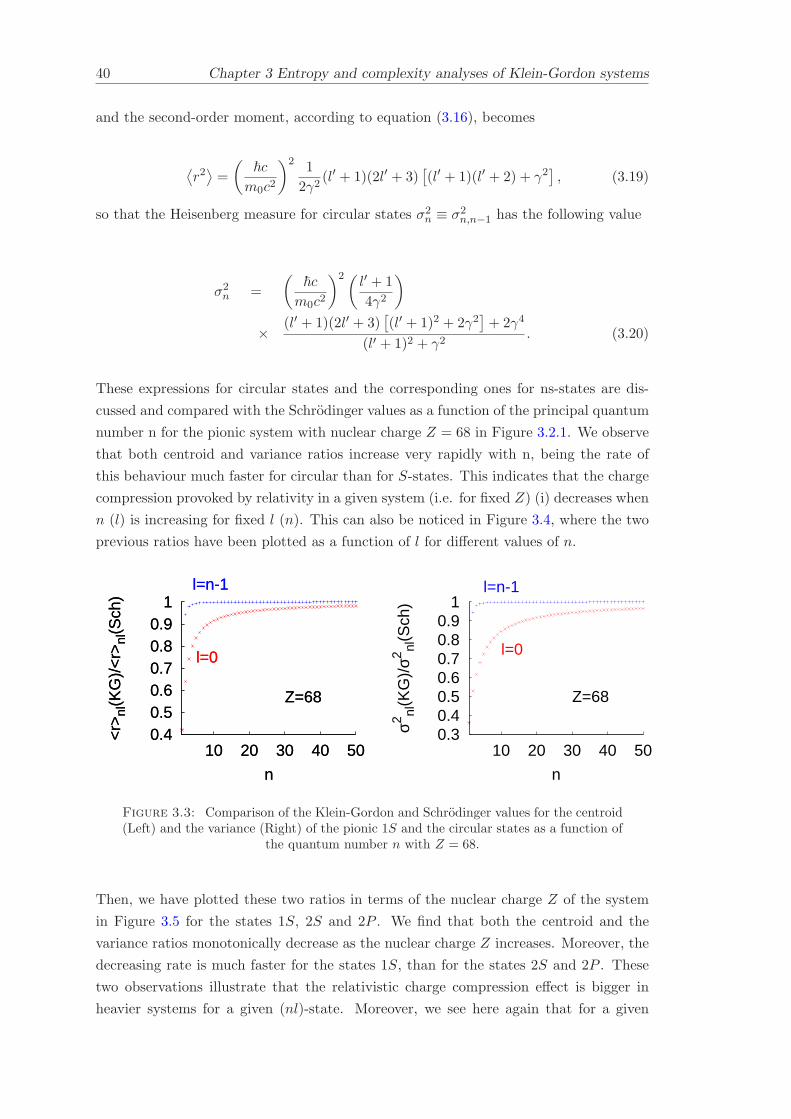
40 Chapter 3 Entropy and complexity analyses of Klein-Gordon systems
and the second-order moment, according to equation (3.16), becomes
⟨r2⟩
=
(~c
m0c2
)2 1
2γ2(l′ + 1)(2l′ + 3)
[(l′ + 1)(l′ + 2) + γ2
], (3.19)
so that the Heisenberg measure for circular states σ2n ≡ σ2
n,n−1 has the following value
σ2n =
(~c
m0c2
)2( l′ + 1
4γ2
)
× (l′ + 1)(2l′ + 3)[(l′ + 1)2 + 2γ2
]+ 2γ4
(l′ + 1)2 + γ2. (3.20)
These expressions for circular states and the corresponding ones for ns-states are dis-
cussed and compared with the Schrodinger values as a function of the principal quantum
number n for the pionic system with nuclear charge Z = 68 in Figure 3.2.1. We observe
that both centroid and variance ratios increase very rapidly with n, being the rate of
this behaviour much faster for circular than for S-states. This indicates that the charge
compression provoked by relativity in a given system (i.e. for fixed Z) (i) decreases when
n (l) is increasing for fixed l (n). This can also be noticed in Figure 3.4, where the two
previous ratios have been plotted as a function of l for different values of n.
0.4 0.5 0.6 0.7 0.8 0.9
1
10 20 30 40 50
<r>
nl(K
G)/
<r>
nl(S
ch)
n
l=0
l=n-1
Z=68
0.4 0.5 0.6 0.7 0.8 0.9
1
10 20 30 40 50
<r>
nl(K
G)/
<r>
nl(S
ch)
n
l=0
l=n-1
Z=68
0.3 0.4 0.5 0.6 0.7 0.8 0.9
1
10 20 30 40 50
σ2 nl(K
G)/
σ2 nl(S
ch)
n
l=0
l=n-1
Z=68
Figure 3.3: Comparison of the Klein-Gordon and Schrodinger values for the centroid(Left) and the variance (Right) of the pionic 1S and the circular states as a function of
the quantum number n with Z = 68.
Then, we have plotted these two ratios in terms of the nuclear charge Z of the system
in Figure 3.5 for the states 1S, 2S and 2P . We find that both the centroid and the
variance ratios monotonically decrease as the nuclear charge Z increases. Moreover, the
decreasing rate is much faster for the states 1S, than for the states 2S and 2P . These
two observations illustrate that the relativistic charge compression effect is bigger in
heavier systems for a given (nl)-state. Moreover, we see here again that for a given

Chapter 3 Entropy and complexity analyses of Klein-Gordon systems 41
0.4 0.5 0.6 0.7 0.8 0.9
1<
r>nl
(KG
)/<
r>nl
(Sch
)
n=1
0.4 0.5 0.6 0.7 0.8 0.9
1<
r>nl
(KG
)/<
r>nl
(Sch
)
n=1
n=2
n=2
n=3
n=3
n=4
n=4
n=5
n=5
n=6
n=6
0.3 0.4 0.5 0.6 0.7 0.8 0.9
1
σ2 nl(K
G)/
σ2 nl(S
ch)
n=1 0.3
0.4 0.5 0.6 0.7 0.8 0.9
1
σ2 nl(K
G)/
σ2 nl(S
ch)
n=1
n=2
n=2
n=3
n=3
n=4
n=4
n=5
n=5
n=6
Figure 3.4: Comparison of the Klein-Gordon and Schrodinger values for the centroid(Left) and the variance (Right), as a function of the quantum number l varying from 0
to n− 1, for different values of n.
0.4 0.5 0.6 0.7 0.8 0.9
1
0 10 20 30 40 50 60
<r>
nl(K
G)/
<r>
nl(S
ch)
Z
n=2 l=1
n=2 l=0
n=1 l=0
0.4 0.5 0.6 0.7 0.8 0.9
1
0 10 20 30 40 50 60
<r>
nl(K
G)/
<r>
nl(S
ch)
Z
n=2 l=1
n=2 l=0
n=1 l=0
0.3 0.4 0.5 0.6 0.7 0.8 0.9
1
0 10 20 30 40 50 60
σ2 nl(K
G)/
σ2 nl(S
ch)
Z
n=2 l=1
n=2 l=0
n=1 l=0
Figure 3.5: Comparison of the Klein-Gordon and Schrodinger values for the centroid(Left) and the variance (Right), as a function of the nuclear charge Z for the pionic
states 1S, 2S and 2P .
system it increases both when n decreases for fixed l and when l decreases for fixed n.
The quantum number m doesn’t affect both ratios because the radial part of the density
is not a function of it.
Finally, let highlight that in all figures the Klein-Gordon values tend towards the Schrodinger
values in the non-relativistic limit of large n or small Z.
3.2.2 Shannon and Fisher information measures
Here we study numerically the relativistic effects on the charge spreading of pionic
systems of hydrogenic type by means of the following information-theoretic measures

42 Chapter 3 Entropy and complexity analyses of Klein-Gordon systems
of the associated charge distribution ρnlm(~r) given by Eq (3.9): The Shannon entropy
power and the Fisher information.
The Shannon entropic power of a negatively-charged Klein-Gordon particle characterized
by the charge density ρnlm(~r) is defined by [15]
Nnlm ≡ N [ρnlm] =1
2πeexp
(2
3Snlm
), (3.21)
where Snlm is the Shannon entropy of ρnlm(~r) given by the expectation value of −log (ρnlm(~r)),
i. e.
Snlm ≡ S [ρnlm] = −∫
R3
ρnlm(~r) log ρnlm(~r)d3r, (3.22)
which quantifies the total extent of the charge spreading of the system. Taking into
account the above-mentioned ansatz for ψ(~r) and Eqs. (3.7), (3.9) and (3.22), this
expression can be separated out into radial and angular parts
Snlm = S [Rnl] + S [Ylm] ,
as it is explained in full detail in [21], being Rnl and Ylm the radial and angular parts
of the density. We should keep in mind that the angular part is the same for both
Klein-Gordon and Schrodinger cases.
The Fisher information is defined by [10]
Inlm ≡ I [ρnlm] =
∫
R3
|∇ρ(~r)|2ρ(~r)
d3r. (3.23)
Remark that we are not using here the parameter dependent Fisher information origi-
nally introduced (and so much used) by statisticians [81], but its translationally invariant
form that does not depend on any parameter; see ref. [10, 82] for further details. It is
worthy to point out that the Fisher information is a measure of the gradient content
of the charge distribution: so, when ρ(~r) has a discontinuity at a certain point, the
local slope value drastically changes and the Fisher information strongly varies. This
indicates that it is a local quantity in contrast to the Heisenberg measure σ2nl and the
Shannon entropy S [ρ] (and its associated power), which have a global character because
they are powerlike and logarithmic functionals of the density, respectively.
Unlike the moment-based quantities discussed in the previous Section, these comple-
mentary measures do not depend on a special point, either the origin as the ordinary
moments or the centroid as the Heisenberg measure. These quantities, first used by
statisticians and electrical engineers and later by quantum physicists, have been shown
to be measures of disorder or smoothness of the density ρnlm(~r) [10, 15]. Let us highlight
that the Fisher information does not only measure the charge spreading of the system
in a complementary and qualitatively different manner as the Heisenberg and Shannon

Chapter 3 Entropy and complexity analyses of Klein-Gordon systems 43
measures but also it quantifies their oscillatory character, indicating the local charge
concentration all over the space [10].
The relativistic (Klein-Gordon) and non-relativistic (Schrodinger) values of the Shannon
entropic power are numerically discussed and compared in Figure 3.6 for the pionic
system. Therein, on the left, we plot the ratio Nnl(KG)/Nnl(Sch) between these two
values as a function of the principal quantum number n for the system with nuclear
charge Z = 68. We notice that the Shannon ratio systematically increases when n is
increasing, approaching to unity for large n, for both circular and S-states. Moreover, we
find that this approach is much faster for circular states, what indicates once more that
the relativistic effects are much more important for states S. In addition, on the right of
Figure 3.6, we show the dependence of the Shannon ratio with the nuclear charge Z for
the 1S, 2S ant 2P states. We observe, here again, that the ratio is a decreasing function
of Z for any state, indicating that the relativistic effects are much more important for
heavy systems. Moreover, for a given system (i.e. fixed Z) the relativistic effects increase
when n (l) decreases for fixed l (n). The quantum number m affects the absolute value
of the Shannon entropic power but it doesn’t affect the ratio.
0
0.2
0.4
0.6
0.8
1
0 5 10 15 20 25
Nnl
(KG
)/N
nl(S
ch)
n
l=n-1
l=0
Z=68
0
0.2
0.4
0.6
0.8
1
0 5 10 15 20 25
Nnl
(KG
)/N
nl(S
ch)
n
l=n-1
l=0
Z=68
0
0.2
0.4
0.6
0.8
1
0 10 20 30 40 50 60
Nnl
(KG
)/N
nl(S
ch)
Z
n=2 l=1
n=2 l=0n=1 l=0
Figure 3.6: Comparison of the Klein-Gordon and Schrodinger values for the Shannonentropic power as a function of the principal quantum number n (Left) and the nuclear
charge Z (Right).
Figure 3.7 shows the dependence of the ratio of the non-relativistic and relativistic
values of the Fisher information for various states with l 6= 0 on their quantum numbers
(n, l,m) for the pionic system with Z = 68 (left graph) and on the nuclear charge Z
(right graph). The Fisher information for S-states is not defined because the involved
integral diverges. First we should remark that here, contrary to the previous quantities
considered in this work, the Schrodinger values are always less than the Klein-Gordon
ones; this is strongly related to the local character of the Fisher information, indicating
that the localized internodal charge concentration is always larger in the relativistic case.
Second, we observe that for fixed l the Fisher ratio Inl(Sch)/Inl(KG) monotonically
increases when n is getting bigger, approaching to unity at a rate which grows as l is

44 Chapter 3 Entropy and complexity analyses of Klein-Gordon systems
0.88
0.92
0.96
1
0 5 10 15 20 25
I nl(S
ch)/
I nl(K
G)
n
l=n-1 m=n-1
l=1 m=1
l=1 m=0
Z=680.88
0.92
0.96
1
0 5 10 15 20 25
I nl(S
ch)/
I nl(K
G)
n
l=n-1 m=n-1
l=1 m=1
l=1 m=0
Z=68
0.84
0.88
0.92
0.96
1
0 10 20 30 40 50 60
I nl(S
ch)/
I nl(K
G)
Z
n=2 l=1 m=0
n=3 l=1 m=0
n=2 l=1 m=1
Figure 3.7: Comparison of the Klein-Gordon and Schrodinger values for the Fisherinformation as a function of the principal quantum number n (Left) and the nuclear
charge Z (Right).
0
0.2
0.4
0.6
0.8
1
Nnl
(KG
)/N
nl(S
ch)
n=1
0
0.2
0.4
0.6
0.8
1
Nnl
(KG
)/N
nl(S
ch)
n=1
n=2
n=2
n=3
n=3
n=4
n=4
n=5
n=5
n=6
n=6
0
0.2
0.4
0.6
0.8
1
I nl(S
ch)/
I nl(K
G)
n=2
0
0.2
0.4
0.6
0.8
1
I nl(S
ch)/
I nl(K
G)
n=2
n=3
n=3
n=4
n=4
n=5
n=5
n=6
Figure 3.8: Comparison of the Klein-Gordon and Schrodinger values for the Shannonentropic power as a function of l varying from 0 to n−1 (Left) and the Fisher information
as a function of l varying from 1 to n− 1 (Right) for different values of n.
increasing. Third, we find that the Fisher ratio decreases for all states in a systematic
way as the nuclear charge increases. Moreover, for a given Z value this ratio increases
as either the quantum numbers n and/or l increase.
For completeness, the behaviour of the Shannon and Fisher ratios in terms of the orbital
quantum number l for a fixed n is more explicitly shown of the left and right graphs,
respectively, of Figure 3.8.
Finally, in Figure 3.9, the dependence of the Fisher ratio on the magnetic quantum
number m is studied. Notice that the ratio is bigger when |m| is increasing, indicating
that the lower |m| is, the more concentrated is the charge density of the state and the
more important are the relativistic effects.

Chapter 3 Entropy and complexity analyses of Klein-Gordon systems 45
0.8
0.85
0.9
0.95
1
I nlm
(KG
)/I n
lm(S
ch)
l=1
0.8
0.85
0.9
0.95
1
I nlm
(KG
)/I n
lm(S
ch)
l=1
l=2
l=2
l=3
l=3
l=4
Figure 3.9: Comparison of the Klein-Gordon and Schrodinger values for the Fisherinformation as a function of m varying from 0 to l, for different values of l.
3.3 Complexity analysis of Klein-Gordon single-particle
systems
Numerous phenomena and properties of many-electron systems have been qualitatively
characterized by information-theoretic means. In particular, various single and com-
posite information-theoretic measures have been proposed to identify and analyse the
multiple facets of the internal disorder of non-relativistic quantum systems; see e.g. Ref.
[11, 13, 14, 46, 63, 83–89].
They are often expressed as products of two quantities of local (e. g. the Fisher infor-
mation) and/or global (e. g. the variance or Heisenberg measure, the Shannon entropy,
the Renyi and Tsallis entropies and the disequilibrium or linear entropy 〈ρ〉) character,
which describe the charge spreading of the system in a complementary and more com-
plete manner than their individual components. This is the case of the disequilibrium-
Shannon or Lopez-Ruiz-Mancini-Calvet (LMC in short) [86], disequilibrium-Heisenberg
[89], Fisher-Shannon [11, 13, 46, 63, 87, 88, 90] and the Cramer-Rao [11, 13, 15, 88]
complexities, which have their minimal values at the extreme ordered and disordered
limits.
Recently these studies have been extended to take into account the relativistic effects in
atomic physics. Relativistic quantum mechanics [70] tells us that special relativity pro-
vokes (at times , severe) spatial modifications of the electron density of many-electron
systems, what produces fundamental and measurable changes in their physical proper-
ties. The qualitative and quantitative evaluation of the relativistic modification of the
spatial redistribution of the electron density of ground and excited states in atomic and
molecular systems by information-theoretic means is a widely open field. In the last
three years the relativistic effects of various single and composite information-theoretic
quantities of the ground states of hydrogenic [55] and neutral atoms [52, 91] have been
investigated in different relativistic settings.
46 Chapter 3 Entropy and complexity analyses of Klein-Gordon systems
First Borgoo et al [52] (see also [92]), in a Dirac-Fock setting, find that the LMC shape
complexity of the ground-state atoms (i) has an increasing dependence on the nuclear
charge (also observed by Katriel and Sen [55] in Dirac ground-state hydrogenic sys-
tems), (ii) manifest shell and relativistic effects, the latter being specially relevant in the
disequilibrium ingredient (which indicates that they are dominated by the innermost
orbital). Then, Sanudo and Lopez-Ruiz [91] (see also [93]) show a similar trend for
both LMC and Fisher-Shannon complexities in a different setting which uses the frac-
tional occupation probabilities of electrons in atomic orbitals instead of the continuous
electronic wavefunctions; so, they use discrete forms for the information-theoretic ingre-
dients of the complexities. Moreover, their results allow to identify the shell structure
of noble gases and the irregular shell filling of some specific elements; this phenomenon
is specially striking in the Fisher-Shannon case as the authors explicitly point out.
The present Section contributes to this new field with the quantification of the relativis-
tic compression of both ground and excited states of the Klein-Gordon single-particle
wavefunctions in a Coulombian well by means of the Fisher-Gordon complexity. This
quantity is defined by
CFS [ρ] := I [ρ] × J [ρ] , (3.24)
where
I [ρ] =
∫ρ(~r)
[d
dxlog ρ (~r)
]2
d~r, J [ρ] =1
2πeexp (2S [ρ] /3) , (3.25)
are the Fisher information and the Shannon entropic power of the density ρ(~r), respec-
tively. The latter quantity, which is an exponential function of the Shannon entropy
S[ρ] = −〈logρ〉, measures the total extent to which the single-particle distribution is
in fact concentrated [15]. The Fisher information I [ρ], which is closely related to the
kinetic energy [82], is a local information-theoretic quantity because it is a gradient
functional of the density, so being sensitive to the single-particle oscillations. Then,
contrary to the remaining complexities published in the literature up until now, the
Fisher-Shannon complexity has a property of locality and it takes simultaneously into
account the spatial extent of the density and its (strong) oscillatory nature.
3.3.1 The Fisher-Shannon measure of pionic systems
Let us now numerically discuss the relativistic effects in the Fisher-Shannon complexity
of a pionic system. First, we center our attention in the dependence on the nuclear
charge of the system. As we can see in Figure 3.10, the Fisher-Shannon complexity of
the Klein-Gordon case depend on the nuclear charge Z, contrary to the non-relativistic
description. The Schrodinger or non-relativistic value of the Fisher-Shannon complexity

Chapter 3 Entropy and complexity analyses of Klein-Gordon systems 47
has been recently shown to be independent of the nuclear charge Z for any hydrogenic
system, It is apparent that this quantity is a very good indicator of the relativistic effects
as has been recently pointed out by Sanudo and Lopez-Ruiz [91, 93] in other relativistic
settings. These effects are bigger when the nuclear charge increases, so the relativistic
Fisher-Shannon complexity enhances. This behaviour is easy to understand because
when we take into account the relativistic effects, the charge probability density is more
compressed towards the nucleus than in the non-relativistic case [70] (see Figure 3.2).
1.3
1.35
1.4
1.45
1.5
1.55
1.6
1.65
0 2 4 6 8 10 12 14 16 18 20
C(F
S)
Z
KG
SCH
Figure 3.10: Fisher-Shannon complexity ratio for the ground state Klein-Gordon(KG) and Schrodinger (SCH) pionic atom in terms of the nuclear charge Z (atomic
units are used).
To measure the relativistic effects we define the quantity ζFS = 1 − CSCH(FS)CKG(FS) . This
quantity varies from 0 to 1, so that ζFS ∼ 0 when the relativistic effects are negligible
and ζFS ∼ 1 in the ultrarelativistic limit. In Figure 3.11 we can see the effects of the
relativity model for different values of the nuclear charge Z and various S(n, 0, 0) states.
0 0.1 0.2 0.3 0.4 0.5 0.6 0.7 0.8 0.9
1
0 2 4 6 8 10 12 14 16 18 20
ζ FS(n
,0,0
)
n
Z=68
Z=50Z=30
Z=1
Figure 3.11: Fisher-Shannon complexity ratio for various S states of the Klein-Gordonand Schrodinger pionic atom.
First, we observe that the relativistic effects increase when the nuclear charge is increa-
sing not only for the ground state (as already pointed out) but also for all the excited
states. Second, the relativistic effects decrease when the principal quantum number is

48 Chapter 3 Entropy and complexity analyses of Klein-Gordon systems
increasing. Third, this decreasing behaviour with n has a strong dependence with Z,
being slower as bigger is the nuclear charge.
0
0.2
0.4
0.6
0.8
1
ζ FS(n
,l,0)
n=1
0
0.2
0.4
0.6
0.8
1
ζ FS(n
,l,0)
n=1
n=2
n=2
n=3
n=3
n=4
n=4
n=5
n=5
n=6
0
0.2
0.4
0.6
0.8
1
ζ FS(n
,l,0)
n=1
0
0.2
0.4
0.6
0.8
1
ζ FS(n
,l,0)
n=1
n=2
n=2
n=3
n=3
n=4
n=4
n=5
n=5
n=6
Figure 3.12: Fisher-Shannon complexity ratio for various states (n, l, 0) of the Klein-Gordon and Schrodinger pionic atoms with Z = 68 (left) and Z = 30 (right).
In Figure 3.12 we can observe that the relativistic effects are practically negligible when
the angular quantum number is different to zero even when the nuclear charge is big.
This dependence in l is more important than the dependence on the principal quantum
number n. For completeness, let us point out that the relativistic effects are practically
negligible when the magnetic quantum number m varies for (Z, n, l) fixed.
3.3.2 The LMC shape complexity of pionic systems
Here we study the LMC shape complexity [86] of the pionic systems defined by Equa-
tion 1.6 in a similar way as done previously with the Fisher-Shannon complexity. The
principal results are given in Figures 3.13, 3.14, 3.15. In Figure 3.13 the values of the
Klein-Gordon (KG) and Schrodinger (SCH) shape complexities for the ground-state pio-
nic atom are shown in terms of the nuclear charge Z. It is apparent that the behaviour of
this measure with the nuclear charge Z is similar to that of the Fisher-Shannon comple-
xity displayed in Figure 3.10. We first observe that, opposite to the Schrodinger setting
(where the shape complexity is constant), the relativistic Klein-Gordon shape comple-
xity varies indeed with Z. This indicates that this measure is also a good indicator of the
relativistic effects. These effects clearly enhance when the nuclear charge is increasing.
This enhancement can be quantified by means of the ratio ζSC = 1 − CSCH(SC)CKG(SC) , whose
value for various states S in terms of the principal quantum number N is given in Figure
3.14 for the pionic systems with nuclear charge Z = 1, 30, 50 and 68. The relativistic
effects manifest much more weakly in the shape complexity than in the Fisher-Shannon
measure. This relative behaviour is mainly due to the fact that the shape complexity
does not grasp the strong oscillatory character of the pionic wavefunctions, while the
Fisher-Shannon complexity really does.
Finally in Figure 3.15 we show the relative behaviour if the shape complexity in the
relativistic Klein-Gordon and non-relativistic cases in terms of the orbital quantum

Chapter 3 Entropy and complexity analyses of Klein-Gordon systems 49
2.5
2.52
2.54
2.56
2.58
2.6
2.62
0 5 10 15 20
C(L
MC
)
Z
Sch
KG
Figure 3.13: Shape complexity for the ground state Klein-Gordon (KG) andSchrodinger (SCH) pionic atom in terms of the nuclear charge Z.
0 0.1 0.2 0.3 0.4 0.5 0.6 0.7 0.8 0.9
1
0 2 4 6 8 10 12 14 16 18 20
ζ SC
(n,0
,0)
n
Z=68
Z=50
Z=30
Z=1
Figure 3.14: Shape complexity for S states of the Klein-Gordon and Schrodingerpionic atom with nuclear charges Z = 1, 30, 50 and 68.
number l for various states (n, l, 0) with fixed n. This behaviour is similar to the
Fisher-Shannon case shown in Figure 3.12. again, we observe that the relativistic effects
are negligible for l other than 0, even for atoms with a large nuclear charge.
0
0.2
0.4
0.6
0.8
1ζSC(n,l,0)
n=1
0
0.2
0.4
0.6
0.8
1ζSC(n,l,0)
n=1
n=2
n=2
n=3
n=3
n=4
n=4
n=5
n=5
n=6
0
0.2
0.4
0.6
0.8
1ζSC(n,l,0)
n=1
0
0.2
0.4
0.6
0.8
1ζSC(n,l,0)
n=1
n=2
n=2
n=3
n=3
n=4
n=4
n=5
n=5
n=6
Figure 3.15: Shape complexity for various states (n, l, 0) of the Klein-Gordon andSchrodinger pionic atoms with Z = 68 (left) and Z = 30 (right).
50 Chapter 3 Entropy and complexity analyses of Klein-Gordon systems
For completeness, let us also point out that the relativistic effects are practically negli-
gible when the magnetic number m varies for pionic states with given quantum numbers
(n, l) of atoms with a nuclear charge Z.
3.4 Conclusions
The relativistic charge compression of spinless Coulomb particles has been quantitatively
investigated by means of the Heisenberg, Shannon and Fisher spreading measures. These
three complementary quantities show that the relativity effects are larger (i. e. the
charge compresses more towards the origin) for the lower energetic states and when the
Coulomb strength (i. e. the nuclear charge Z) increases. Moreover, a detailed analysis
of these quantities on the quantum numbers (n, l,m) characterising the physical states
of a given system (i. e. for a fixed Z) indicate that the relativistic effects increase
when n (l) decreases for fixed l (n). Furthermore, the study of the Fisher information
shows that the relativistic effects also increase when the magnetic quantum number |m|is increasing for fixed (n, l).
We have explored relativistic effects on the behaviour of the Fisher-Shannon comple-
xity of pionic systems with nuclear charge Z in the Klein-Gordon framework too. We
have done it for both ground and excited states. First we found that the relativistic
Fisher-Shannon complexity grows when the nuclear charge increases, in contrast with
the non-relativistic case for both ground and excited states. A similar behaviour has
been recently observed in the case of the ground state of systems governed by the Dirac
equation [52, 91–93]. We found that this trend remains for excited states in a damped
way, so that the relativistic effects enhance with Z for a given (n, l,m) state and, for a
given Z, decrease when the principal and/or orbital quantum numbers are increasing.
Let us also highlight that the non-relativistic limits at large principal quantum number
n for a given Z (see Figs. 3.11 and 3.12) and at small values of Z (see Fig. 3.10) are
reached. On the other hand it is pertinent to underline that the finite nuclear volume
effects are very tiny for any information-theoretic and complexity measure because of
its macroscopic character.
We have also investigated the relativistic Klein-Gordon effects in pionic atoms by means
of the LMC shape complexity [86] C(LMC) = 〈ρ〉 expS [ρ]. We found that the relativistic
effects are also identified by this quantity but in a much weaker way than the Fisher-
Shannon complexity C(FS). Apparently this is because of the property of locality of
C(FS) coming through its gradient-dependent Fisher ingredient, which grasps much
better the (strong) oscillatory condition of the pionic densities.

Chapter 4
Information-theoretic lengths of
orthogonal polynomials
Let pn(x) denote a sequence of real orthonormal polynomials with respect to the
weight function ω(x) on the interval ∆ ≡ (a, b) ⊆ R (see e.g. [94, 95]), i.e.
∫
∆pn(x)pm(x)ω(x)dx = δn,m, m, n ∈ N (4.1)
The distribution of these polynomials along the orthogonality interval can be comple-
mentarity measured by means of the spreading properties of the normalized-to-unity
density function
ρn(x) ≡ ρ[pn] = p2n(x)ω(x), (4.2)
which is called Rakhmanov’s density of the polynomial pn(x), to honour the pioneering
work [96] of this mathematician who has shown that this density governs the asymp-
totic (n → ∞) behaviour of the ratio pn+1/pn. Physically, this probability density
characterizes the stationary states of a large class of quantum-mechanical potentials
[94]. Beyond the variance, the spreading of the orthogonal polynomials is best analy-
sed by the information-theoretic properties of their associated Rakhmanov probability
densities; namely, the Fisher information [81], the Renyi entropy [97] and the Shannon
entropy [2].
The information-theoretic knowledge of the orthogonal polynomials is reviewed in Ref
[24] up to 2001, where the quantum-mechanical motivation and some physical appli-
cations are also given, and up today in [98], where emphasis is made on asymptotics.
Therein, it is pointed out that the study of the information-theoretic measures of ortho-
gonal polynomials was initiated in the nineties with the asymptotic computation of the
Renyi and Shannon entropies of the classical orthogonal polynomials [99–101]. Up until
now, however, the explicit expressions of these two spreading measures are not known
51

52 Chapter 4 Information-theoretic lengths of orthogonal polynomials
save for the Shannon measure for some particular subclasses of the Jacobi polynomials;
namely the Chebyshev polynomials of first and second type [100, 101] and the Gegen-
bauer polynomials C(λ)n (x) with integer parameter λ [102, 103]. On the other hand, the
Fisher information for all classical orthogonal polynomials on a real interval (Hermite,
Laguerre, Jacobi) has been calculated in a closed form in 2005 [104]. This has allowed
us to find, more recently, the Cramer-Rao information plane (i.e. the plane defined by
both the Fisher information and the variance) for these systems [105].
This Chapter has two main purposes. First, in Section 4.1 to introduce a more ap-
propriate set of spreading measures (to be called information-theoretic-based spreading
lengths of Renyi, Shannon and Fisher types) in the field of orthogonal polynomials.
The spreading lengths are direct measures of position spread of the variable x, as the
root-mean-square or standard deviation ∆x. So, they have the following properties:
same units as x, invariance under translations and reflections, linear scaling with x and
vanishing in the limit as ρn(x) approaches a delta function. The second purpose is to
compute all these lengths for the Hermite (see Section 4.2) and Laguerre polynomials
4.3. In each case we first compute their moments around the origin and, as well, the
standard deviation of these objects. Then we compute the entropic or frequency mo-
ments [106–108] of these polynomials by means of the Bell polynomials, so useful in
Combinatorics [109, 110], in the Hermite and Laguerre case and, alternatively, by the
linearization technique of Srivastava-Niukkanen in the Laguerre case. This achievement
allows us to obtain the Renyi lengths of Hermite and Laguerre polynomials by means of
an efficient algorithm based on the known properties of Bell’s polynomials. With respect
to the Shannon length, since its explicit expression cannot be determined, we obtain its
asymptotics and we derive a family of sharp upper bounds by use of an information-
theoretic-based optimization procedure. Moreover, the Fisher information is explicitly
calculated. Finally, these information-theoretic quantities are applied to the compu-
tation of the spreading lengths of the main quantum-mechanical prototype of physical
systems: the harmonic oscillator.
4.1 Spreading lengths of classical orthogonal polynomials
Here we shall refer to the hypergeometric-type polynomials, i.e. the polynomials pn(x)defined by the orthogonality relation given by Eq. (4.1). It is well-known that they
can be reduced to one of the three classical families of Hermite, Jacobi and Laguerre by
appropriate linear changes of the variable [94]. The spreading of these polynomials along
their orthogonality interval ∆ ≡ (a, b) can be measured by means of (i) the moments
around a particular point of the orthogonality interval; usually it is chosen the origin
(moments around the origin: µ′k =⟨xk⟩n) or the centroid 〈x〉 (central moments or
moments around the centroid: µk = 〈(x−〈x〉n)k〉n) [111] and (ii) the frequency moments
Wk[ρn] := 〈[ρn(x)]k〉 [107, 111, 112] of the associated Rakhmanov density ρn(x) given

Chapter 4 Information-theoretic lengths of orthogonal polynomials 53
by Eq. (4.2). The symbol 〈f(x)〉 ≡ 〈f(x)〉n denotes the expectation value of f(x) with
respect to the density ρn(x) as
〈f(x)〉n :=
∫
∆f(x)ρn(x)dx =
∫
∆f(x)ω(x)p2
n(x)dx.
These two classes of ordinary and frequency moments are complementary spreading
measures of global type. While the ordinary moments measures the distribution of the
probability with respect to a particular point of the support interval ∆, the frequency
moments measure the extent to which the probability is in fact distributed. So it happens
that the latter moments are, at times, much better probability estimators than the
ordinary ones [107, 108]. Moreover, they are fairly efficient in the range where the
ordinary moments are fairly inefficient [106]; see also the brief, recent summary about
these quantities done in Ref. [113]. Therein we learn that the frequency moments are
also called ”entropic moments” because they are closely connected to the Renyi entropies
[97]
Rq[ρn] :=1
1 − qlog〈[ρn(x)]q−1〉; q > 0; q 6= 1, (4.3)
and the Tsallis entropies [114]
Tq[ρn] :=1
q − 1
[1 − 〈[ρn(x)]q−1〉
]; q > 0; q 6= 1, (4.4)
as well as to other information-theoretic quantities, such as the Brukner-Zeilinger en-
tropy [115] and the linear entropy [116].
Among the first class of moments we highlight the familiar root-mean-square or standard
deviation (∆x)n given by
(∆x)n =(⟨x2⟩n− 〈x〉2n
) 12,
because it is a direct measure of spreading [72] in the sense of having the same units as
the variable, and has various interesting properties: invariance under translations and
reflections, linear scaling (i.e., ∆y = λ∆x for y = λx) and vanishing as the density
approaches a Dirac delta density (i.e. in the limit that x tends towards a given definite
value).
From the second class of moments we fix our attention on the Renyi lengths [72] defined
by
LRq [ρn] ≡ exp (Rq[ρn]) = 〈[ρn(x)]q−1〉−1
q−1 =
∫
∆dx[ρn(x)]q
− 1q−1
, q > 0, q 6= 1,
(4.5)
which are not only direct spreading measures but also have the three above-mentioned
properties of the standard deviation. Among them we highlight the second-order Renyi

54 Chapter 4 Information-theoretic lengths of orthogonal polynomials
length (also called Onicescu information [8], Heller length [117], disequilibrium [4, 6] and
inverse participation ratio in other contexts [118, 119])
L[ρn] := LR2 [ρn] = 〈ρn(x)〉−1 =
∫
∆dx[ρn(x)]2
−1
,
and, above all, the Shannon length [2, 72]
N [ρn] := limq→1
LRq [ρn] = exp (S[ρn]) ≡ exp
[−∫
∆dxρn(x) log ρn(x)
],
where S[ρn] is the Shannon information entropy [2].
There exists a third class of spreading measures for the classical orthogonal polynomials,
which are qualitatively different in the sense that, in contrast to the previous ones, they
have a local character. Indeed they are functionals of the derivative of the associated
Rakhmanov density ρn(x), so that they are very sensitive to local rearrangements of
the variable. The most distinctive measure of this class is the so-called Fisher length
[81, 120, 121] defined by
(δx)n :=1√F [ρn]
≡⟨[
d
dxlog ρn(x)
]2⟩− 1
2
=
∫
∆dx
[ρ′n(x)]2
ρn(x)
− 12
, (4.6)
where F [ρn] denotes the Fisher information of the classical orthogonal polynomials [104].
This quantity measures the pointwise concentration of the probability along the orthogo-
nality interval, and quantifies the gradient content of the Rakhmanov density providing
(i) a quantitative estimation of the oscillatory character of the density and of the poly-
nomials and (ii) the bias to particular points of the interval, so that it measures the
degree of local disorder.
It is worthy to remark that the Fisher length, as the Heisenberg and Renyi lengths, is
a direct spreading measure and has the three properties of translation and reflection
invariance, linear scaling and vanishing when the density tends to a delta density. In
addition, the Fisher length is finite for all distributions [120]. Moreover, the direct
spreading measures just mentioned have an uncertainty/certainty property: see Refs.
[72] for the Heisenberg, Shannon and Renyi cases, and [122, 123] for the Fisher case.
Finally, they fulfil the inequalities [72]
(δx)n ≤ (∆x)n, and N [ρn] ≤ (2πe)12 (∆x)n, (4.7)
where the equality is reached if and only if ρn(x) is a Gaussian density.

Chapter 4 Information-theoretic lengths of orthogonal polynomials 55
4.2 Spreading lengths of Hermite polynomials
In this section we calculate the moments-with-respect-to-the-origin 〈xk〉, k ∈ Z, the
entropic moments Wq[ρn] ≡ 〈[ρn(x)]q〉, of integer order q, and the Renyi, Shannon
and Fisher spreading lengths of the Rakhmanov density of the orthonormal Hermite
polynomials Hn(x) given by
Hn(x) =
n∑
l=0
clxl, (4.8)
with
cl =(−1)
3n−l2 n!
(2nn!√π)
12
2l(n−l2
)!l!
(−1)l + (−1)n
2, (4.9)
where the last factor vanishes when l and n have opposite parities. These polynomials are
known to fulfil the orthonormality relation (4.1) with the weight function ωH(x) = e−x2
on the whole real line [94, 95]. Thus, according to Eq. (4.2), the expression
ρn(x) ≡ ρ[Hn](x) = e−x2H2n(x) (4.10)
gives the Rakhmanov density of the orthonormal Hermite polynomial Hn(x).
4.2.1 Ordinary moments and the standard deviation
The moments of the Hermite polynomials Hn(x) are defined by the moments of its
associated Rakhmanov density (4.2); that is
〈xk〉n :=
∫ ∞
−∞xkH2
n(x)e−x2dx, k = 0, 1, 2, . . . (4.11)
The use of (4.8), (4.1) and (4.11) gives
〈xk〉n =
k!2kΓ( k
2+1) 2F1
(−n,−k
2
1
∣∣∣∣∣ 2), even k
0, odd k
, (4.12)
which can be also obtained from some tabulated special integrals [124].
In the particular cases k = 0, 1 and 2 we obtain the first few moments around the origin:
〈x0〉n = 1, 〈x〉n = 0, 〈x2〉n = n+1
2,
so that the second central moment of the density
(∆x)n =√〈x2〉n − 〈x〉2n =
√n+
1
2(4.13)

56 Chapter 4 Information-theoretic lengths of orthogonal polynomials
describes the standard deviation.
4.2.2 Entropic moments and Renyi lengths of integer order q
The qth-order frequency or entropic moment of the Hermite polynomials Hn(x) is defined
by the corresponding quantity of its associated Rakhmanov density given by Eq. (4.2);
that is,
Wq[ρn] =⟨ρnq−1
⟩=
∫ ∞
−∞ρn(x)q dx =
∫ ∞
−∞e−qx
2Hn(x)2qdx; q ≥ 1 (4.14)
The evaluation of this quantity in a closed form is not at all a trivial task despite
numerous efforts published in the literature [125, 126] save for some special cases. Here
we will do it by means of the Bell polynomials which play a relevant role in Combinatorics
[127, 128]. We start from the explicit expression (4.8) for the Hermite polynomial Hn(x);
then, taking into account the Appendix C we have that its pth-power can be written
down as
[Hn(x)]p =
[n∑
k=0
ckxk
]p=
np∑
k=0
p!
(k + p)!Bk+p,p(c0, 2!c1, . . . , (k + 1)!ck)x
k, (4.15)
with ci = 0 for i > n, and the remaining coefficients are given by Eq. (4.9). Moreover,
the Bell polynomials are given by
Bm,l(c1, c2, . . . , cm−l+1) =∑
π(m,l)
m!
j1!j2! · · · jm−l+1!
(c11!
)j1 (c22!
)j2· · ·(
cm−l+1
(m− l + 1)!
)jm−l+1
(4.16)
where the sum runs over all partitions π(m, l) such that
j1 + j2 + · · · + jm−l+1 = l, and j1 + 2j2 + · · · + (m− l + 1)jm−l+1 = m. (4.17)
The substitution of the expression (4.15) with p = 2q into Eq. (4.14) yields the value
Wq[ρn] =
2nq∑
k=0
(2q)!
(k + 2q)!Bk+2q,2q(c0, 2!c1, . . . , (k + 1)!ck)
∫ ∞
−∞e−qx
2xkdx
=
nq∑
j=0
Γ(j + 1
2
)
qj+12
(2q)!
(2j + 2q)!B2j+2q,2q(c0, 2!c1, . . . , (2j + 1)!c2j), (4.18)
where the parameters ci are given by Eq. (4.9), keeping in mind that ci = 0 for every
i > n, so that the only non-vanishing terms correspond to those with ji+1 = 0 so that

Chapter 4 Information-theoretic lengths of orthogonal polynomials 57
cji+1
i = 1 for every i > n. In the particular cases q = 1 and 2, we obtain the value
W1[ρn] =
∫ ∞
−∞ρn(x)dx = 1
for the normalization of ρn(x), as one would expect, and
W2[ρn] =
∫ ∞
−∞ρn(x)2 dx =
∫ ∞
−∞e−2x2
(Hn(x))4dx
=2n∑
j=0
Γ(j + 1
2
)
2j+12
4!
(2j + 4)!B2j+4,4(c0, 2!c1, . . . , (2j + 1)!c2j) (4.19)
for the second-order entropic moment.
As well, the entropic moments of arbitrary order q for the Hermite polynomials of lowest
degree (e.g., n = 0, 1 and 2) have the values
Wq[ρ0] =
√π1−q
q, Wq[ρ1] =
2q
πq2 qq+
12
Γ
(q +
1
2
), Wq[ρ2] =
π1−q2 2q(2q)!
q2q+12
L(−2q− 1
2)
2q
(−q
2
),
where L(α)n (x) denotes a Laguerre polynomial.
Then, we can now calculate all the information-theoretic measures of the Hermite poly-
nomials which are based on their entropic moments Wq[ρn] just calculated, such as the
Renyi and Tsallis entropies given by Eqs. (4.3) and (4.4), respectively, and the Brukner-
Zeilinger and linear entropy which are closely related to the first-order entropic moment
W2[Hn] given by Eq. (4.19). Particularly relevant are the values
LRq [ρn] = Wq[ρn]−1
q−1 = (4.20)
=
nq∑
j=0
Γ(j + 1
2
)
qj+12
(2q)!
(2j + 2q)!B2j+2q,2q(c0, 2!c1, . . . , (2j + 1)!c2j)
− 1q−1
; q = 2, 3, . . .
for the Renyi lengths (4.5) of Hermite polynomials, and
L[ρn] = W2[ρn]−1 =
2n∑
j=0
Γ(j + 1
2
)
2j+12
4!
(2j + 4)!B2j+4,4(c0, 2!c1, . . . , (2j + 1)!c2j)
−1
,
for the Heller length of Hermite polynomials.
Let us just explicitly write down the values
LRq [ρ0] = π12 q
12(q−1)
LRq [ρ1] =
(π
12 q
2
) qq−1
q1
2(q−1)
(Γ
(q +
1
2
))− 1q−1

58 Chapter 4 Information-theoretic lengths of orthogonal polynomials
LRq [ρ2] = π12 2
q1−q q
4q+12q−2
((2q)!L
(−2q− 12)
2q
(−q
2
))− 1q−1
for the Renyi lengths of the first few Hermite polynomials with lowest degrees, and the
values
L[ρ0] =√
2π, L[ρ1] =4
3
√2π, L[ρ2] =
64
41
√2π
for the Onicescu-Heller length of these polynomials.
4.2.3 Shannon length: Asymptotics and sharp bounds
Here we determine the asymptotics of the Shannon length N [ρn] of the Hermite polyno-
mials Hn(x) and its relation with its standard deviation. Moreover we use an information-
theoretic-based optimization procedure to find sharp upper bounds to N [ρn] and we
discuss their behaviour in a numerical way.
The Shannon length or exponential entropy of the Hermite polynomials Hn(x) is defined
by
N [ρn] = exp S[ρn] , (4.21)
where
S[ρn] = −∫ ∞
−∞e−x
2H2n(x) log
[e−x
2H2n(x)
]dx (4.22)
is the Shannon entropy of the Hermite polynomial of degree n. Simple algebraic opera-
tions yield to
S[ρn] = n+1
2−∫ ∞
−∞e−x
2H2n(x) log H2
n(x)dx (4.23)
The logarithmic integral involved in this expression has not yet been determined in spite
of serious attempts for various authors [99–101, 129]. Nevertheless these authors have
found its value for large n by use of the strong asymptotics of Hermite polynomials; it
is given as
∫ ∞
−∞e−x
2H2n(x) log H2
n(x)dx = n+3
2− log π − log
√2n+ o(1). (4.24)
Then, from (4.23) and (4.24) one has the asymptotical value
S[ρn] = log√
2n+ log π − 1 + o(1) = logπ√
2n
e+ o(1)
for the Shannon entropy, and
N [ρn] ≃ π√
2n
e; n≫ 1 (4.25)

Chapter 4 Information-theoretic lengths of orthogonal polynomials 59
for the Shannon length of the Hermite polynomial Hn(x). From Eqs. (4.13) and (4.25)
one finds the following relation
N [ρn] ≃ π√
2
e(∆x)n; n≫ 1 (4.26)
between the asymptotical values of the Shannon length and the standard deviation of
the Hermite polynomial Hn [130]. Remark that this relation fulfils the general inequality
(4.7) which mutually relate the Shannon length and the standard deviation.
Since the evaluation of the Shannon S(Hn) given by Eq. (4.23) is not yet possible for a
generic degree, it seems natural to try to find sharp bounds to this quantity. Here we do
that by use of the non-negativity of the Kullback-Leibler entropy of the two arbitrary
probability densities ρ(x) and f(x) defined by
IKL[ρ, f ] =
∫ ∞
−∞ρ(x) log
ρ(x)
f(x)dx.
Indeed, for ρ(x) = ρn(x), the Rakhmanov density (4.2) associated to the Hermite poly-
nomials, the non-negativity of the corresponding Kullback-Leibler functional yields the
following upper bound to S(Hn):
S[ρn] ≤ −∫ ∞
−∞ρn(x) log f(x)dx, (4.27)
Then we make the choice
f(x) =ka
1k
2Γ(
1k
)e−xk, k = 2, 4, . . . (4.28)
duly normalized to unity, as prior density, The optimization of the upper bound (4.27)
for the choice (4.28) with respect to the parameter a yields the following optimal bound
S[ρn] ≤ log
[Ak〈xk〉
1kn
], k = 2, 4, . . .
with the constant
Ak =2(ek)
1k
kΓ
(1
k
).
Finally, taking into account the expectation values 〈xk〉n of the Rakhmanov density ρn
of the Hermite polynomial Hn(x) given by Eq. (4.12), we have that
S[ρn] ≤ log
(ek)
1k
kΓ
(1
k
)[k!
Γ(k2 + 1
) 2F1
(−n,−k
2
1
∣∣∣∣∣ 2)] 1
k
,
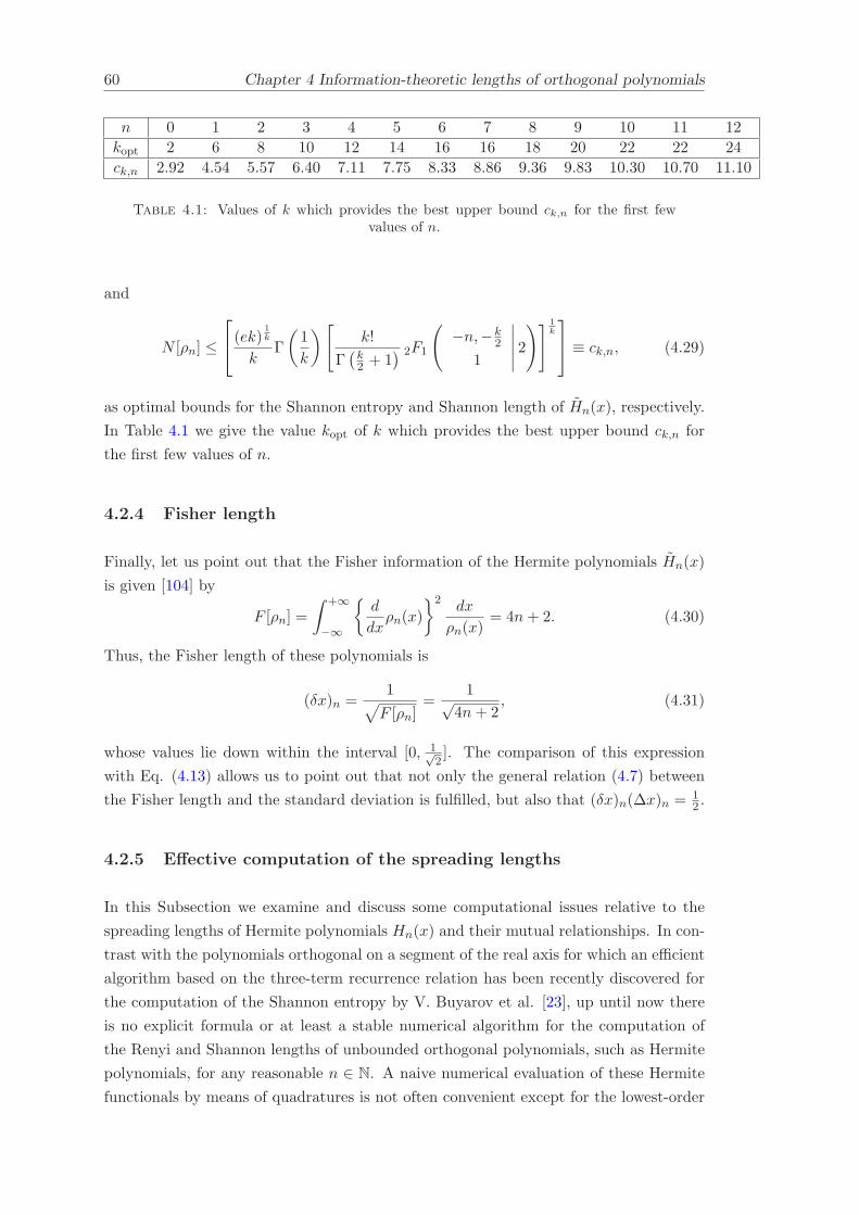
60 Chapter 4 Information-theoretic lengths of orthogonal polynomials
n 0 1 2 3 4 5 6 7 8 9 10 11 12
kopt 2 6 8 10 12 14 16 16 18 20 22 22 24
ck,n 2.92 4.54 5.57 6.40 7.11 7.75 8.33 8.86 9.36 9.83 10.30 10.70 11.10
Table 4.1: Values of k which provides the best upper bound ck,n for the first fewvalues of n.
and
N [ρn] ≤
(ek)
1k
kΓ
(1
k
)[k!
Γ(k2 + 1
) 2F1
(−n,−k
2
1
∣∣∣∣∣ 2)] 1
k
≡ ck,n, (4.29)
as optimal bounds for the Shannon entropy and Shannon length of Hn(x), respectively.
In Table 4.1 we give the value kopt of k which provides the best upper bound ck,n for
the first few values of n.
4.2.4 Fisher length
Finally, let us point out that the Fisher information of the Hermite polynomials Hn(x)
is given [104] by
F [ρn] =
∫ +∞
−∞
d
dxρn(x)
2 dx
ρn(x)= 4n+ 2. (4.30)
Thus, the Fisher length of these polynomials is
(δx)n =1√F [ρn]
=1√
4n+ 2, (4.31)
whose values lie down within the interval [0, 1√2]. The comparison of this expression
with Eq. (4.13) allows us to point out that not only the general relation (4.7) between
the Fisher length and the standard deviation is fulfilled, but also that (δx)n(∆x)n = 12 .
4.2.5 Effective computation of the spreading lengths
In this Subsection we examine and discuss some computational issues relative to the
spreading lengths of Hermite polynomials Hn(x) and their mutual relationships. In con-
trast with the polynomials orthogonal on a segment of the real axis for which an efficient
algorithm based on the three-term recurrence relation has been recently discovered for
the computation of the Shannon entropy by V. Buyarov et al. [23], up until now there
is no explicit formula or at least a stable numerical algorithm for the computation of
the Renyi and Shannon lengths of unbounded orthogonal polynomials, such as Hermite
polynomials, for any reasonable n ∈ N. A naive numerical evaluation of these Hermite
functionals by means of quadratures is not often convenient except for the lowest-order

Chapter 4 Information-theoretic lengths of orthogonal polynomials 61
2
4
6
8
10
12
14
16
0 20 40 60 80 100
LRq [ρn]
n
Figure 4.1: Renyi lengths LRq [ρn] with q = 2 (+), 3 (⊙), 4 (×), and 5 (⊡), in terms
of the degree n.
polynomials since the increasing number of integrable singularities spoils any attempt
to achieve a reasonable accuracy for arbitrary n.
We propose an analytical, error-free and easily programmable computing approach for
the entropic moments Wq[ρn] and the Renyi spreading lengths LRq [ρn] of the orthonor-
mal polynomials Hn(x), which are given by Eqs. (4.18) and (4.21), respectively, in
terms of the combinatorial multivariable Bell polynomials defined by Eq. (4.16). This
approach requires the knowledge of the expansion coefficients cl given by Eq. (4.9) and
the determination of the partitions π(m, l) given by Eq. (4.17).
In Figures 4.1 and 4.2 we have shown the Renyi lengths LRq [ρn] with q = 2, 3, 4 and
5, and the Shannon length N [ρn] of the orthonormal Hermite polynomials in terms of
the degree n within the range n ∈ [0, 100], respectively. We observe that both Shannon
and Renyi lengths with fixed q have an increasing parabolic dependence on the degree
n of the polynomials. Moreover, this behaviour is such that for fixed n the Renyi length
decreases when q is increasing. As well, in Figure 4.2 we plot the optimal upper bound
ckopt,n for the Shannon length N [ρn] according to Eq. (4.29).
Finally, for completeness, we have numerically studied the relation of the Shannon length
N [ρn] and the Onicescu-Heller length L[ρn] of these polynomials with the standard
deviation (∆x)n within the range n ∈ [0, 100]. The corresponding results are shown
in Figures 4.3 and 4.4, respectively. We observe that when n varies from 0 to 100 the
two spreading lengths have a quasilinear behaviour in terms of the standard deviation.
Moreover, we found the fit
N [ρn] = 1.723(∆x)n + 2.00 (4.32)

62 Chapter 4 Information-theoretic lengths of orthogonal polynomials
0
5
10
15
20
25
30
0 20 40 60 80 100
N [ρn]
ckopt,n
n
Figure 4.2: Shannon length N [ρn] (×) and its optimal upper bound ckopt,n (⊙) interms of the degree n.
for the Shannon length, with a correlation coefficient R = 0.999998, and
L[ρn] = 1.204(∆x)n + 2.92,
for the Onicescu-Heller length or second-order Renyi length with a correlation coeffi-
cient R = 0.99994. In fact, the global dependence of N [ρn] on (∆x)n is slightly con-
cave, being only asymptotically linear according to the rigorous expression (4.26), i.e.
N [ρn] ≃ π√
2e (∆x)n ≃ 1.63445(∆x)n for n≫ 1, which is in accordance with (4.32). It is
worthwhile remarking (i) the nα behaviour with α > 0 of the global spreading lengths
(standard deviation, Renyi and Shannon lengths) and (ii) the n−12 -law which is followed
by the (local) Fisher length. This difference may be associated to the gradient-functional
form (4.6) of the Fisher length, indicating a locality property in the sense that it is very
sensitive to the oscillatory character of the polynomials.
4.2.6 Application
The states of the one-dimensional harmonic oscillator, with a potential V (x) = 12λ
2x2,
are determined by the following probability density
ρHOn (x) =
√λ
2nn!√πe−λx
2(Hn(
√λx))2
whereHn(x) are the orthogonal Hermite polynomials [94]. Since Hn(x) = (2nn!√π)−
12Hn(x),
this density can be expressed in terms of the Rakhmanov density of the orthonormal

Chapter 4 Information-theoretic lengths of orthogonal polynomials 63
2
4
6
8
10
12
14
16
0 1 2 3 4 5 6 7 8 9 10 11
LRq [ρn]
(∆x)n
Figure 4.3: Renyi lengths LRq [ρn] with q = 2 (+), 3 (⊙), 4 (×), and 5 (⊡), in terms
of the standard deviation (∆x)n for n ∈ [0, 100].
2
4
6
8
10
12
14
16
18
20
0 1 2 3 4 5 6 7 8 9 10 11
N [ρn]
(∆x)n
Figure 4.4: Shannon length N [ρn] in terms of the standard deviation (∆x)n forn ∈ [0, 100].
Hermite polynomials Hn(x) defined by Eq. (4.10) as follows:
ρHOn (x) =
√λρn(
√λx).
Taking this into account, we obtain for the harmonic oscillator the following expressions
〈xk〉HOn = λ−
k2 〈xk〉n; k = 0, 1, 2, . . .
Wq[ρHOn ] = λ
q−12 Wq[ρn]; q = 0, 1, 2, . . .

64 Chapter 4 Information-theoretic lengths of orthogonal polynomials
for the ordinary and entropic moments, and
S[ρHOn ] = − log
√λ+ S[ρn],
F [ρHOn ] = λF [ρn],
for the Shannon and Fisher information measures in terms of the corresponding quanti-
ties of the Hermite polynomials, whose values are given by Eqs. (4.12), (4.18), (4.23) and
(4.30), respectively. Then, it is straightforward to find that all the uncertainty measures
of the harmonic oscillator (namely, standard deviation and Renyi, Shannon and Fisher
lengths) are equal, save for a multiplication factor λ−12 , to the corresponding spreading
lengths of the Hermite polynomials which control their wavefunctions. This is to say
that
(∆x)HOn = λ−
12 (∆x)n, LRq [ρHO
n ] = λ−12LRq [ρn]
N [ρHOn ] = λ−
12N [ρn], (δx)HO
n = λ−12 (δx)n,
whose values can be obtained by keeping in mind Eqs. (4.13), (4.21)-(4.23), and (4.31)
respectively.
4.2.7 Open problems
Here we want to pose the following unsolved problems: to find the asymptotics of the
frequency or entropic moments Wq[ρn] defined by
Wq[ρn] =
∫ ∞
−∞
[ωH(x)H2
n(x)]qdx =
∫ ∞
−∞e−qx
2[Hn(x)
]2qdx, q ≥ 1 (4.33)
in the two following cases:
• n→ ∞, and q ∈ R fixed.
• q → ∞, and n ∈ N fixed.(4.34)
Up until now the only known result is due to A. Aptekarev et al [98, 99, 129] who have
shown that these quantities, which are weighted L2q-norms of the orthonormal Hermite
polynomials Hn(x) as
Wq[ρn] =‖ Hn(x) ‖2q2q,
behave asymptotically (n→ ∞) as
Wq[ρn] =
(2
π
)q Γ(q + 1
2
)Γ(1 − q
2
)
Γ(q + 1)Γ(
32 − q
2
) (2n+ 1)1−q2 (1 + o(1))

Chapter 4 Information-theoretic lengths of orthogonal polynomials 65
when q ∈ [0, 43 ]. To extend and generalize this result in the sense mentioned above,
it might be useful for the interested reader to keep in mind the two following related
results:
(a) L. Larsson-Cohn [131] studied the Lp-norms of the monic Hermite polynomials
hn(x), orthogonal with respect to the Gaussian weight ωG(x) = (2π)−12 exp
(−x2
2
),
defined by
‖h‖p =
(1
2π
) p2∫ ∞
−∞e−
x2
2 |hn(x)|pdx 1
p
.
Keeping in mind that ‖h‖n =√n!, he found the following asymptotical (n → ∞)
result
‖h‖p =
c(p)n−
14
√n!(1 +O(n−1)), if 0 < p < 2
c(p)n−14
√n!(p− 1)
n2 (1 +O(n−1)), if 2 < p <∞
with the values
c(p) =
(2π
) 14
(2
2−p
) 12p
Γ( p+1
2 )√πΓ( p+2
2 )
1p
, for p < 2
(2π
) 14
(p−12p−4
) p−12p, for p > 2
However, the asymptotics of the entropic moments Wq[hn] of the Hermite polyno-
mials hn(x) defined by
Wq[hn] =
∫ ∞
−∞
[ωG(x)h2
n(x)]qdx =
(1
2π
) q2∫ ∞
−∞e−
q2x2
[hn(x)]2q dx (4.35)
has not yet been found.
(b) R. Azor et al [125] have used combinatorial techniques for the asymptotics (n→ ∞)
of the following functionals of the Hermite polynomials Hn(x) orthogonal with
respect to e−x2:
Zk[Hn] :=
∫ ∞
−∞e−x
2[Hn(x)]kdx, k ∈ N.
They were only able to solve it in the particular non-trivial case k = 4, where
Z4[Hn] =3
4n
√3
π
62n
(n!)2
1 − 1
4n+
3
16n2+O(n−3)
.
Besides, they have also considered the asymptotics (k → ∞) of Zk[Hn] as well as
that of the quantities
Dk[Hn] :=
√2
π
∫ ∞
−∞e−2x2
[Hn(x)
]kdx,

66 Chapter 4 Information-theoretic lengths of orthogonal polynomials
finding the following results
Zk[Hn] ∼[1 + (−1)kn
] (2kn−1π
) 12
(kn
e
) kn2
e−n−1
2 , for k ≫ 1
Dk[Hn] ∼ 1 + (−1)kn√2
(kn
e
) kn2
e−(n−1), for k ≫ 1
The solution of the problems (4.33)-(4.34) and/or (4.35), and the full determination
of the asymptotics of Zk[Hn] and Dk[Hn] for (n → ∞, k ∈ R), either by means of
an approximation-theoretic methodology [98, 99, 129, 131] or by use of combinatorial
techniques [125, 126], is of great relevance from both mathematical and applied points of
view from obvious reasons, keeping in mind the physico-mathematical meaning of these
quantities as previously mentioned. It is worthwhile remarking that, in particular, the
quantity Wq[ρn] is not only the (2q)th-power of the L2q-norm of the Hermite polynomials
but it also represents the entropic moment of order q of the harmonic oscillator and their
isospectral physical systems, which fully determines the Renyi and Tsallis entropies of
these objects.
4.3 Direct spreading measures of Laguerre polynomials
The Laguerre polynomialsL
(α)n (x)
are real hypergeometric polynomials orthonormal
with respect to the weight function ωα(x) = xαe−x on the interval [−1, 1]. They play
a crucial role in numerous branches of applied mathematics [132–134], mathematical
physics [94, 95], quantum physics [135]. This is mainly because their algebraic pro-
perties (orthogonality relation, three-term recurrence relation, second-order differential
equation, ladder relation,...) are simple and widely known [94, 132, 133], which have
allowed us to describe a great deal of scientific and technological phenomena. Let us
just mention that the Laguerre polynomials appear in the wavefunctions which describe
the quantum states of one and many-body systems with a great diversity of quantum-
mechanical potentials in ordinary [135–140] and supersymmetric [141] quantum mecha-
nics. The Coulomb and Morse potentials are only two particularly relevant cases in
atomic and molecular physics (see e.g. [136, 138, 142–144] as well as in D-dimensional
physics [145], where the radial wavefunctions are controlled by Laguerre polynomials.
In this work we study the spreading measures of Laguerre polynomials L(α)n , which
quantify the distribution of its Rakhmanov associated probability density
ρn,α(x) =1
d2n
[L(α)n (x)
]2ωα(x), (4.36)
where d2n is a normalization constant. Physically, this probability density characterizes
the stationary states of a large class of quantum-mechanical potentials [94, 136, 137,
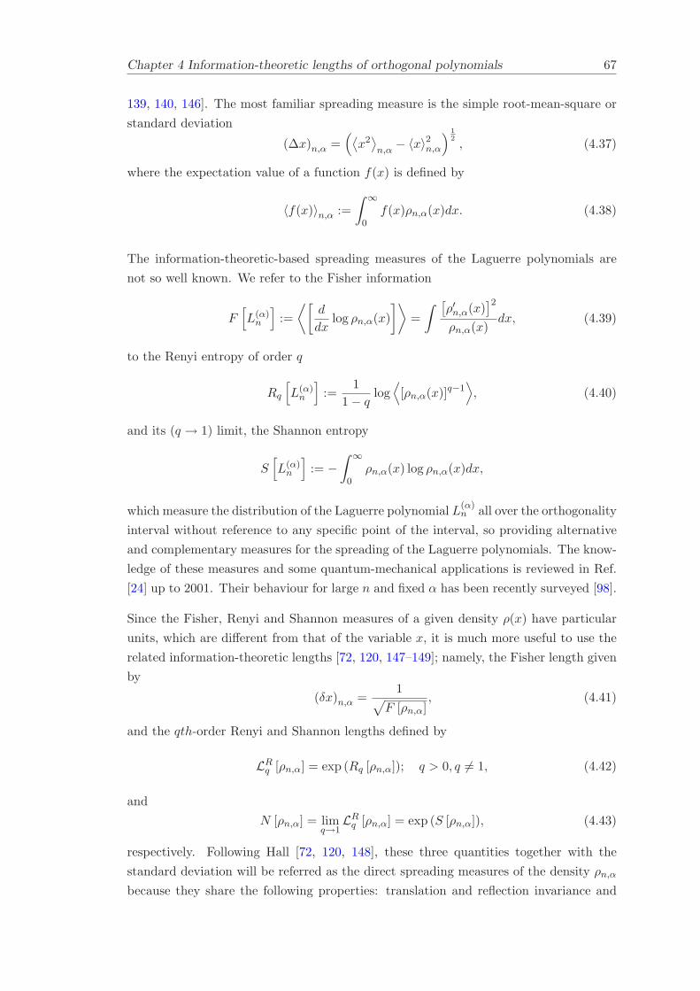
Chapter 4 Information-theoretic lengths of orthogonal polynomials 67
139, 140, 146]. The most familiar spreading measure is the simple root-mean-square or
standard deviation
(∆x)n,α =(⟨x2⟩n,α
− 〈x〉2n,α) 1
2, (4.37)
where the expectation value of a function f(x) is defined by
〈f(x)〉n,α :=
∫ ∞
0f(x)ρn,α(x)dx. (4.38)
The information-theoretic-based spreading measures of the Laguerre polynomials are
not so well known. We refer to the Fisher information
F[L(α)n
]:=
⟨[d
dxlog ρn,α(x)
]⟩=
∫ [ρ′n,α(x)
]2
ρn,α(x)dx, (4.39)
to the Renyi entropy of order q
Rq
[L(α)n
]:=
1
1 − qlog⟨
[ρn,α(x)]q−1⟩, (4.40)
and its (q → 1) limit, the Shannon entropy
S[L(α)n
]:= −
∫ ∞
0ρn,α(x) log ρn,α(x)dx,
which measure the distribution of the Laguerre polynomial L(α)n all over the orthogonality
interval without reference to any specific point of the interval, so providing alternative
and complementary measures for the spreading of the Laguerre polynomials. The know-
ledge of these measures and some quantum-mechanical applications is reviewed in Ref.
[24] up to 2001. Their behaviour for large n and fixed α has been recently surveyed [98].
Since the Fisher, Renyi and Shannon measures of a given density ρ(x) have particular
units, which are different from that of the variable x, it is much more useful to use the
related information-theoretic lengths [72, 120, 147–149]; namely, the Fisher length given
by
(δx)n,α =1√
F [ρn,α], (4.41)
and the qth-order Renyi and Shannon lengths defined by
LRq [ρn,α] = exp (Rq [ρn,α]); q > 0, q 6= 1, (4.42)
and
N [ρn,α] = limq→1
LRq [ρn,α] = exp (S [ρn,α]), (4.43)
respectively. Following Hall [72, 120, 148], these three quantities together with the
standard deviation will be referred as the direct spreading measures of the density ρn,α
because they share the following properties: translation and reflection invariance and

68 Chapter 4 Information-theoretic lengths of orthogonal polynomials
linear scaling under adequate boundary conditions, same units as the variable, and
vanishing when the density tends to a delta density. Moreover, they have an associated
uncertainty property [72, 120, 123, 148] and fulfil the inequalities
(δx)n,α ≤ (∆x)n,α and N [ρn,α] ≤ (2πe)12 (∆x)n,α . (4.44)
Here we will investigate the direct spreading measures of the Laguerre polynomials
mentioned above. First, in Subsection 4.3.1, we give the known values of the ordinary
moments, the standard deviation and the Fisher length of these polynomials. Second, in
Subsection 4.3.2, the entropic moments⟨
[ρn,α(x)]k⟩
and the Renyi lengths are computed
by use of two different approaches; one makes use of the Srivastava-Niukkanen lineari-
zation relation [150] of Laguerre polynomials, and another one which is based on the
combinatorial multivariable Bell polynomials [128, 149]. Third, in Subsection 4.3.3, the
asymptotics of the Shannon length is given and some sharp bounds to this measure are
found. Then, in Subsection 4.3.4, all the four spreading measures are computationally
discussed. Finally, some open problems and conclusions are given.
4.3.1 Ordinary moments, standard deviation and Fisher length
In this section the known values for the moments-around-the-origin⟨xk⟩n,α
(k ∈ Z), the
standard deviation (∆x)n,α and the Fisher length (δx)n,α of the Laguerre polynomials
are given. Let us start writing the orthonormality relation
∫ ∞
0L(α)n (x)L(α)
m (x)ωα(x)dx = δnm,
for the orthonormal Laguerre polynomials
L(α)n (x) =
[n!
Γ(α+ n+ 1)
] 12
L(α)n (x). (4.45)
Then, the moment-around-the-origin of order k ∈ Z is defined, according to Eq. (4.38),
by ⟨xk⟩
n,α=
∫ ∞
0xkρn,α(x)dx =
∫ ∞
0xk+αe−x
[L(α)n (x)
]2dx.
This integral can be calculated by different means; in particular, by use of the expression
[37, 80, 151–153]
∫ ∞
0xse−xL(α)
n (x)L(β)m (x)dx = Γ(s+ 1)
min(n,m)∑
r=0
(−1)n+m
(s− α
n− r
)(s− β
m− r
)(s+ r
r
),

Chapter 4 Information-theoretic lengths of orthogonal polynomials 69
one finds that
⟨xk⟩
n,α=n!Γ(k + α+ 1)
Γ(n+ α+ 1)
n∑
r=0
(k
n− r
)2(k + α+ r
r
),
where the binomial number is(ab
)= Γ(a+1)
Γ(b+1)Γ(a−b+1) . Then, taking into account Eq. (4.37)
and the values⟨xk⟩n,α
for k = 1, 2, one has the following expression for the standard
deviation of the Laguerre polynomials [105]
(∆x)n,α =√
2n2 + 2(α+ 1)n+ α+ 1. (4.46)
The Fisher information of the Laguerre polynomials defined by Eq. (4.39) has been
recently shown [104] to have the value
F(L(α)n
)=
4n+ 1; α = 0,(2n+1)α+1
α2−1; α > 1,
∞; α ∈ (−1,+1], α 6= 0,
so that the Fisher length of these polynomials has, according to (4.41), the value
(δx)n,α =
1√4n+1
; α = 0,√
α2−1(2n+1)α+1 ; α > 1,
0; α ∈ (−1,+1], α 6= 0.
It is worth remarking that the inequality (δx)n,α ≤ (∆x)n,α is clearly satisfied.
4.3.2 Renyi lengths
In this section the Renyi lengths of the Laguerre polynomials LRq [ρn,α] defined by Eq.
(4.42) will be computed by two different approaches: an algebraic approach which is
based on the Srivastava-Niukkanen linearization relation [150], and a combinatorial
method which utilizes the multivariable Bell polynomials [128].
According to Eqs. (4.40) and (4.42), the Renyi length of order q is given by
LRq [ρn,α] = Wq [ρn,α]−1
q−1 , q > 0, q 6= 1, (4.47)
where
Wq [ρn,α] :=⟨
[ρn,α(x)]q−1⟩
=
∫ ∞
0[ρn,α(x)]q dx =
∫ ∞
0
[Lαn(x)
]2qxqαe−qxdx, (4.48)

70 Chapter 4 Information-theoretic lengths of orthogonal polynomials
are the frequency or entropic moments of the Rakhmanov density (4.36) of the Laguerre
polynomials. In spite of the efforts of numerous researchers [126, 132, 154–156], these
quantities have not yet been calculated. Here we will compute them by use of two
different approaches.
4.3.2.1 Algebraic approach
To calculate the entropic moment Wq [ρn,α], we first use (4.45) and (4.48) to write
Wq [ρn,α] :=
[n!
Γ(α+ n+ 1)
]qIq
[L(α)n
], (4.49)
where
Iq
[L(α)n
]:=
∫ ∞
0xαqe−qx
[L(α)n (x)
]2qdx. (4.50)
This functional of the orthogonal Laguerre polynomial can be calculated by use of the
linearization formula of Srivastava-Niukkanen [150] for the products of various Laguerre
polynomials given by
xµL(α1)m1
(t1x) · · ·L(αr)mr
(trx) =∞∑
k=0
Θk (µ; t1, · · · , tr)L(β)k (x),
where the coefficients Θk (µ;x1, · · · , xr) can be expressed as
Θk (µ; t1, · · · , tr) = (β + 1)µ(m1+α1
m1
)· · ·(mr+αr
mr
)
×F (r+1)A [β + µ+ 1,−m1, · · · ,−mr,−k;α1 + 1, · · · , αr + 1, β + 1; t1, · · · , tr, 1] ,
in terms of the Lauricella’s hypergeometric functions of (r + 1) variables [157]. The
Pochhammer symbol is (a)n = Γ(a+n)Γ(a) . This general relation with the values (β = 0,
α1 = · · · = αr = α, m1 = · · · = mr = n, x = qt, t1 = · · · = tr = 1q , µ = αq, r = 2q)
readily yields the following linearization result for the powers of Laguerre polynomials:
(qt)2q[L(α)n (t)
]2q=
∞∑
k=0
Θk
(αq;
1
q, · · · , 1
q
)L
(0)k (qt), (4.51)
where
Θk
(αq;
1
q, · · · , 1
q
)= Γ(αq + 1)
(n+ α
n
)2q
× F(2q+1)A
(αq + 1;−n, · · · ,−n;−k;α+ 1 · · · , α+ 1, 1;
1
q, · · · , 1
q, 1
).
Taking into account (4.50), (4.51) and the orthogonality relation of the polynomials
L(α)n (x), one finally has that the term with k = 0 is the only non-vanishing contribution

Chapter 4 Information-theoretic lengths of orthogonal polynomials 71
to Iq
[L
(α)n
], so that
Iq
[L(α)n
]=
1
qαq+1Θ0
(αq;
1
q, · · · , 1
q
), (4.52)
with
Θ0 = Γ(αq + 1)(n+αn
)2q
×F (2q+1)A
(αq + 1;−n, · · · ,−n; 0;α+ 1, · · · , α+ 1, 1; 1
q , · · · , 1q , 1). (4.53)
Then, the entropic moments of the Laguerre polynomials have, according to Eqs. (4.49)
and (4.52), the following expresion
Wq [ρn,α] =
[n!
Γ(α+ n+ 1)
]q 1
qαq+1Θ0
(αq;
1
q, · · · , 1
q
). (4.54)
Finally, from Eqs. (4.47), (4.53) and (4.54) one has that the Renyi entropy of order q
of the Laguerre polynomials is given by
LRq [ρn,α] =
[(n!
Γ(α+ n+ 1)
)q 1
qαq+1Θ0
(αq;
1
q, · · · , 1
q
)]− 1q−1
=
[(n!
Γ(α+ n+ 1)
)q 1
qαq+1Γ(αq + 1)
(n+ α
n
)2q
×F (2q+1)A
(αq + 1,−n, · · · ,−n, 0;α+ 1, ..., α+ 1, 1;
1
q, · · · , 1
q, 1
)]− 1q−1
,
for every q > 0, q 6= 1. Some examples follow:
• For n = 0
LRq [ρ0,α] =
[1
Γ(α+ 1)qΓ(αq + 1)
qαq+1
]− 1q−1
.
• For n = 1
LRq [ρ1,α] =
[Γ(αq + 1)(α+ 1)2q
Γ(α+ 2)qqαq+1(−(1 + α)q)−2qU(−2q,−(2 + α)q,−(1 + α)q)
]− 1q−1
where U(a, b, z) is a Tricomi confluent hypergeometric function [158].
4.3.2.2 Combinatorial approach
In this approach we begin with the explicit expression of the Laguerre polynomials given
by
L(α)n (x) =
n∑
k=0
ckxk,

72 Chapter 4 Information-theoretic lengths of orthogonal polynomials
with
ck =
√Γ(n+ α+ 1)
n!
(−1)k
Γ(α+ k + 1)
(n
k
), (4.55)
Recently ([149]; see appendix B) it has been found that an integer power of a polynomial
can be expressed by use of the multivariable Bell polynomials of Combinatorics [128].
This result applied to the Laguerre polynomials gives
[L(α)n (x)
]p=
np∑
k=0
p!
(k + p)!Bk+p,p(c0, 2!c1, ..., (k + 1)!ck)x
k, (4.56)
with ci = 0 for i > n, and the remaining coefficients are given by Eq. (4.55). Moreover,
the Bell polynomials are given by
Bm,l(c1, c2, . . . , cm−l+1) =∑
π(m,l)
m!
j1!j2! · · · jm−l+1!
(c11!
)j1 (c22!
)j2· · ·(
cm−l+1
(m− l + 1)!
)jm−l+1
,
where the sum runs over all partitions π(m, l) such that
j1 + j2 + · · · + jm−l+1 = l, and j1 + 2j2 + · · · + (m− l + 1)jm−l+1 = m.
The replacement of expression (4.56) with p = 2q into Eq. (4.48) yields the value
Wq[ρn,α] =
2nq∑
k=0
(2q)!
(k + 2q)!Bk+2q,2q(c0, 2!c1, . . . , (k + 1)!ck)
∫ ∞
0xqαe−qxxkdx =
=
2nq∑
j=0
Γ(αq + k + 1)
qαq+k+1
(2q)!
(k + 2q)!Bk+2q,2q (c0, 2!c1, ..., (k + 1)!ck) , (4.57)
where the parameters ci are given by Eq. (4.55), keeping in mind that ci = 0 for every
i > n, so that the only non-vanishing terms correspond to those with ji+1 = 0 so that
cji+1
i = 1 for every i > n.
It is worthwhile to check that for q = 1 one has that
W1 [ρn,α] =
∫ ∞
0ρn,α(x)dx = 1,
and that for q = 2 we have
W2 [ρn,α] =
4n∑
k=0
Γ(2α+ k + 1)
22α+k+1
24
(k + 4)!Bk+4,4 (c0, 2!c1, ..., (k + 1)!ck) ,
for the Onicescu information [8] of the Laguerre polynomials. Finally, from Eqs. (4.47)
and (4.57) one has the following alternative expression for the qth-order Renyi length of

Chapter 4 Information-theoretic lengths of orthogonal polynomials 73
the Laguerre polynomial for q = 2, 3, . . .,
LRq [ρn,α] =
2nq∑
j=0
Γ(αq + k + 1)
qαq+k+1
(2q)!
(k + 2q)!Bk+2q,2q (c0, 2!c1, ..., (k + 1)!ck)
− 1q−1
,
which for q = 2 yields the value
LR2 [ρn,α] =
[4n∑
n=0
Γ(2α+ k + 1)
22α+k+1
24
(k + 4)!Bk+4,4 (c0, 2!c1, ..., (k + 1)!ck)
]−1
,
for the Onicescu or second-order Renyi length [8] of the Laguerre polynomials.
With these expressions we obtain the same values of LRq [ρ0,α] and LRq [ρ1,α] as in the
previous subsection.
4.3.3 Shannon length: Asymptotics and sharp bounds
The goal of this Subsection is twofold. First, to study the asymptotics of the Shannon
spreading length N [ρn,α] of the orthonormal Laguerre polynomials L(α)n and its relation
to the standard deviation (∆x)n,α. Second, to find sharp upper bounds to N [ρn,α] by
use of an information-theoretic optimization procedure.
Although many results have been recently published in the literature (see e.g. [159,
160]) about the asymptotics of the Laguerre polynomials themselves, they have not yet
been successfully used to obtain the asymptotics of functionals of these mathematical
functions beyond the Lp-norm method of Aptekarev et al [44, 99]. Here we use the
results provided by this method to fix the asymptotics of the Shannon length of these
polynomials and its relation to the standard deviation. From Eq. (4.43) we have that
N [ρn,α] = exp (S [ρn,α]), (4.58)
where
S [ρn,α] := −∫ ∞
0ωα(x)
[L(α)n (x)
]2log
ωα(x)
[L(α)n (x)
]2dx = En
[L(α)n
]+ Jn
[L(α)n
],
with the following entropic functionals [24, 161]
En
[L(α)n
]= −
∫ ∞
0ωα(x)
[L(α)n (x)
]2log[L(α)n (x)
]2dx, (4.59)
and
Jn
[L(α)n
]= −
∫ ∞
0ωα(x)
[L(α)n (x)
]2logωα(x)dx = 2n+α+ 1−αψ (α+ n+ 1) . (4.60)

74 Chapter 4 Information-theoretic lengths of orthogonal polynomials
Moreover, the use to the Lp-norm method of Aptekarev et al [99] has permitted to find
[24] the following values for the asymptotics of En
[L
(α)n
]
En
[L(α)n
]= −2n+ (α+ 1) log (n) − α− 2 + log (2π) + o(1). (4.61)
Then, according to Eqs. (4.59), (4.60) and (4.61), one has that the asymptotical be-
haviour
S [ρn,α] = (α+ 1) log(n) − αψ(α+ n+ 1) − 1 + log(2π) + o(1),
for the Shannon entropy, and
N [ρn,α] ≃ 2πnα+1e−αψ(α+n+1)−1, (4.62)
for the Shannon length of the orthonormal Laguerre polynomials. Moreover, from Eqs.
(4.46) and (4.62) one finds that
N [ρn,α] ≃ π√
2
e(∆x)n,α ; n >> 1, (4.63)
between the asymptotical values of the Shannon length and the standard deviation of
the polynomial L(α)n . It is worth noting that this relation fulfils the general inequality
(4.44) which mutually relates the Shannon length and the standard deviation for general
densities. Moreover, the relation (4.63) for the Rakhmanov densities of Laguerre poly-
nomials is also satisfied by the Rakhmanov densities of Hermite (See Eq. 4.26) [130, 149]
and Jacobi [130, 147] polynomials.
Let us now find sharp upper bounds to the Shannon length N [ρn,α] by taking into
account the non-negativity of the relative Shannon entropy (also called Kullback-Leibler
entropy) of two arbitrary probability densities ρ(x) and f(x). This yields that the
Shannon entropy of ρ(x) is bounded from above by means of
S [ρn,α] ≤ −∫ ∞
0ρ(x) log f(x)dx.
For ρ(x) = ρn,α(x) this expression produces an infinite set of upper bounds to the
Shannon entropy of Laguerre polynomials. The choice of f(x) in the form
f(x) =ba
1+mb
Γ(
1+mb
)xme−axb; m > −1, a > 0, b ∈ N
+, 0 ≤ x <∞, (4.64)
(which is normalized to unity) followed by the optimization of the upper bound with
respect to the parameter a gives rise to
S [ρn,α] ≤ logΓ(β)eβ
bββ〈xb〉β −m〈log x〉; b > 0, m > −1, β =
1 +m
b, (4.65)

Chapter 4 Information-theoretic lengths of orthogonal polynomials 75
following the lines of Refs [28, 162]. Then, according to Eqs. (4.58) and (4.65), we have
the following set of infinite sharp bounds
N [ρn,α] ≤ Γ (β) eβ
bββ
⟨xb⟩βe−m〈log x〉; m > −1, b > 0, (4.66)
for the Shannon length of the Laguerre polynomial L(α)n (x). For m = 0 we have the
upper bound
N [ρn,α] ≤ Γ(
1b
)(be)
1b
b
⟨xb⟩ 1
b, b > 0. (4.67)
This bound is particularly interesting because it only depends on the expectation value⟨xb⟩; the expectation value 〈log x〉 is, at times, unavailable or difficult to evaluate.
4.3.4 Some computational issues
In this section we study various computational issues of the direct spreading measures
of Laguerre polynomials. It is worth pointing out that there is no stable numerical al-
gorithm for the computation of the Renyi and Shannon lengths of these polynomials in
contrast to the case of orthogonal polynomials on a finite interval for which an efficient
algorithm based on the three-term recurrence relation has been recently found by Bu-
yarov et al [23]. Moreover, a naive numerical evaluation of these Laguerre functionals
by means of quadratures is not often convenient except for the lowest-order polynomials
since the increasing number of integrable singularities spoils any attempt to achieve a
reasonable accuracy for arbitrary n. Here we carry out the following numerical study.
First, we examine the numerical accuracy of the optimal bounds (4.66) and (4.67) to the
Shannon length of the Laguerre polynomials L(α)n (x), α fixed, for various degrees n by
taking into account the optimal values of the parameter b in (4.67) and the optimal va-
lues of (b,m) in (4.66). Second, we study the mutual comparison of Fisher, Shannon and
Onicescu lengths and the standard deviation of L(α)n (x) for fixed α and various degrees
n. Finally, we discuss the correlation of the Shannon length N(L(α)n ) and the standard
deviation (∆x)n for various pairs (n, α), which allow us to find, at times, linear relations
between their components.
In Figure 4.5 it is numerically studied the accuracy of the bounds (4.66) and (4.67) to
the Shannon length of the Laguerre polynomial L(α=0)n (x) given by the optimal values
(bopt, 0) in (4.67). This is done by comparing the corresponding optimal bounds with the
“numerically exact” value of the lengths N [ρn,0] for the polynomials with degree n from
0 to 10. The graph on the right of the figure gives the relative ratio of the bound given by
Eq. (4.67) with b = bopt, and the ratio of the bound given by Eq. (4.66) with b = bopt and
m = mopt. Notice that the latter bound is always better than the former, as we have the
parameter m to adjust. The values of optimal pairs (bopt, 0) and (bopt,mopt) are shown
in Tables 4.2 and 4.3, respectively. Note that the optimum value bopt is different when
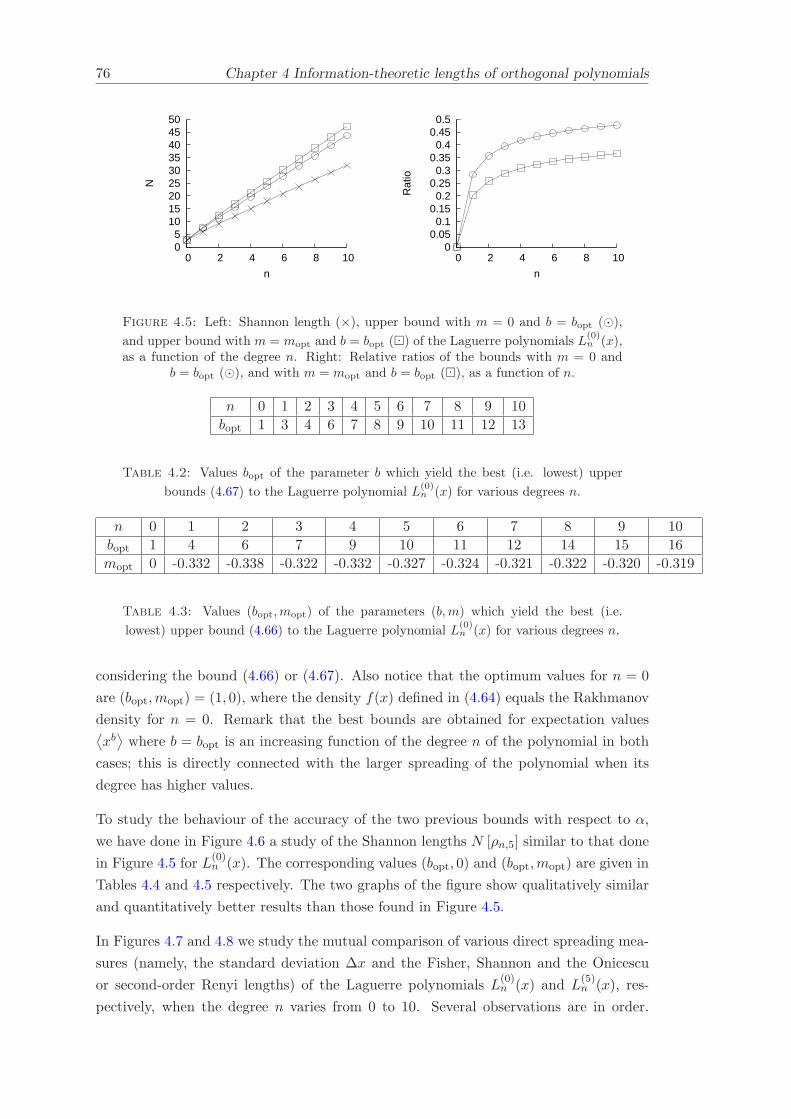
76 Chapter 4 Information-theoretic lengths of orthogonal polynomials
0 5
10 15 20 25 30 35 40 45 50
0 2 4 6 8 10
N
n
0 0.05 0.1
0.15 0.2
0.25 0.3
0.35 0.4
0.45 0.5
0 2 4 6 8 10
Rat
io
n
Figure 4.5: Left: Shannon length (×), upper bound with m = 0 and b = bopt (⊙),
and upper bound with m = mopt and b = bopt (⊡) of the Laguerre polynomials L(0)n (x),
as a function of the degree n. Right: Relative ratios of the bounds with m = 0 andb = bopt (⊙), and with m = mopt and b = bopt (⊡), as a function of n.
n 0 1 2 3 4 5 6 7 8 9 10
bopt 1 3 4 6 7 8 9 10 11 12 13
Table 4.2: Values bopt of the parameter b which yield the best (i.e. lowest) upper
bounds (4.67) to the Laguerre polynomial L(0)n (x) for various degrees n.
n 0 1 2 3 4 5 6 7 8 9 10
bopt 1 4 6 7 9 10 11 12 14 15 16
mopt 0 -0.332 -0.338 -0.322 -0.332 -0.327 -0.324 -0.321 -0.322 -0.320 -0.319
Table 4.3: Values (bopt,mopt) of the parameters (b,m) which yield the best (i.e.
lowest) upper bound (4.66) to the Laguerre polynomial L(0)n (x) for various degrees n.
considering the bound (4.66) or (4.67). Also notice that the optimum values for n = 0
are (bopt,mopt) = (1, 0), where the density f(x) defined in (4.64) equals the Rakhmanov
density for n = 0. Remark that the best bounds are obtained for expectation values⟨xb⟩
where b = bopt is an increasing function of the degree n of the polynomial in both
cases; this is directly connected with the larger spreading of the polynomial when its
degree has higher values.
To study the behaviour of the accuracy of the two previous bounds with respect to α,
we have done in Figure 4.6 a study of the Shannon lengths N [ρn,5] similar to that done
in Figure 4.5 for L(0)n (x). The corresponding values (bopt, 0) and (bopt,mopt) are given in
Tables 4.4 and 4.5 respectively. The two graphs of the figure show qualitatively similar
and quantitatively better results than those found in Figure 4.5.
In Figures 4.7 and 4.8 we study the mutual comparison of various direct spreading mea-
sures (namely, the standard deviation ∆x and the Fisher, Shannon and the Onicescu
or second-order Renyi lengths) of the Laguerre polynomials L(0)n (x) and L
(5)n (x), res-
pectively, when the degree n varies from 0 to 10. Several observations are in order.

Chapter 4 Information-theoretic lengths of orthogonal polynomials 77
5 10 15 20 25 30 35 40 45 50 55 60
0 2 4 6 8 10
N
n
0 0.05 0.1
0.15 0.2
0.25 0.3
0.35 0.4
0.45
0 2 4 6 8 10
Rat
io
n
Figure 4.6: Left: Shannon length (×), upper bound with m = 0 and b = bopt (⊙),
and upper bound with m = mopt and b = bopt (⊡) of the Laguerre polynomials L(5)n (x),
as a function of the degree n. Right: Relative ratios of the bounds with m = 0 andb = bopt (⊙), and with m = mopt and b = bopt (⊡), as a function of n.
n 0 1 2 3 4 5 6 7 8 9 10
bopt 5 6 7 8 10 11 12 13 14 15 16
Table 4.4: Values bopt of the parameter b which yield the best (i.e. lowest) upper
bounds (4.67) to the Laguerre polynomial L(5)n (x) for various degrees n.
n 0 1 2 3 4 5 6 7 8 9 10
bopt 1 5 7 9 10 11 13 14 15 16 17
mopt 5 0.288 0.053 -0.049 -0.098 -0.131 -0.160 -0.177 -0.190 -0.201 -0.210
Table 4.5: Values (bopt,mopt) of the parameters (b,m) which yield the best (i.e.
lowest) upper bound (4.66) to the Laguerre polynomial L(5)n (x) for various degrees n.
First, all the measures with global character (standard deviation, Shannon and Renyi
lengths) grow linearly or quasilinearly when the degree of the polynomial is increasing;
essentially because the polynomial spreads more and more. Moreover, they behave so
that ∆x < L2 < N . Second, the (local) Fisher length decreases when the degree n is
increasing; essentially, because the polynomial becomes more and more oscillatory, so
growing its gradient content. Third, the Fisher length has always a value smaller than
all the global spreading measures.
Finally, in Figure 4.9 we have numerically studied the connection of the Shannon length
N [ρn,α] and the standard deviation (∆x)n,α of the Laguerre polynomials L(α)n (x), with
α = 0 and 5, when the degree n varies from 0 to 20. We obtain the fits
N [ρn,0] = 1.9144(∆x)n + 3.611, (4.68)
and
N [ρn,5] = 1.8951(∆x)n + 5.966, (4.69)

78 Chapter 4 Information-theoretic lengths of orthogonal polynomials
0
5
10
15
20
25
30
35
0 2 4 6 8 10
Spr
eadi
ng L
engh
ts
n
Figure 4.7: Standard deviation ∆x (+), Fisher length δx (×), Onicescu length L2
(⊡), and Shannon length N (⊙) of the Laguerre polynomial L(0)n (x) as a function of n.
0 5
10 15 20 25 30 35 40 45
0 2 4 6 8 10
Spr
eadi
ng L
engh
ts
n
Figure 4.8: Standard deviation ∆x (+), Fisher length δx (×), Onicescu length L2
(⊡), and Shannon length N (⊙) of the Laguerre polynomial L(5)n (x) as a function of n.
for data with n ≥ 10, and correlation coefficient R = 0.9999 in both cases. This apparent
quasilinear behaviour of the Shannon length with respect to the standard deviation is,
in fact, slightly concave, being linear only asymptotically in accordance to the rigorous
expression (4.63), i.e. N[L
(α)n
]≃ 1.63445 (∆x)n,α for n >> 1, which is very close to
(4.68) and (4.69).

Chapter 4 Information-theoretic lengths of orthogonal polynomials 79
0
10
20
30
40
50
60
70
0 5 10 15 20 25 30 35
N
∆x
Figure 4.9: Shannon length N as a function of the standard deviation ∆x for the
Laguerre polynomials L(0)n (x) (+) and L
(5)n (x) (⊡), when the degree n varies from 0 to
20.
4.4 Conclusions
In this Chapter we have introduced new direct measures of orthogonal-polynomials
spreading other than the root-mean-square or standard deviation ∆x which have an
information-theoretic origin; namely, the Renyi, Shannon and Fisher length. They
share with ∆x various interesting properties: same units as the variable, invariance
under translations and reflections, linear scaling, vanishing in the limit that the variable
tends towards a given definite value, and global character. In contrast with ∆x, they do
not depend on any particular point of the orthogonality interval what allow them to be
considered as proper spreading lengths. The Renyi and Shannon lengths are powerlike
and logarithmic functionals of the polynomial pn(x) while Fisher length is a gradient
functional of it, what allows one to state that the former lengths are global measures
and the latter one has a locality property.
In Section 4.2 we have developed a computational methodology for the Renyi length of
the orthonormal Hermite polynomials Hn(x) which is based on the combinatorial multi-
variable Bell polynomials whose arguments are controlled by the expansion coefficients
of Hn(x). For the Shannon length of these polynomials, since it cannot be calculated
explicitly, we give (i) its asymptotics and the relation with the standard deviation, and
(ii) sharp upper bounds by means of an information-theoretic-based optimization pro-
cedure. Moreover, it is computationally found that the second-order Renyi length (also
called Onicescu-Heller length) and the Shannon length linearly depend on the standard
deviation of the polynomials. On the other hand, the Fisher length is analytically shown
to have a reciprocal behaviour with ∆x, mainly because of its local character.

80 Chapter 4 Information-theoretic lengths of orthogonal polynomials
The previous results have been applied to the quantum-mechanical harmonic oscillator
and some open problems related to the asymptotics of the frequency or entropic moments
of Hermite polynomials are posed. Their solution would allow not only to complete this
work but also to extend considerably the related findings of various authors in connection
to the Lp-norms of Hermite polynomials [98, 99, 125, 129, 131].
In Section 4.3 the direct spreading measures of the Laguerre polynomials L(α)n (x) are
analytically and numerically studied. Beyond the ordinary moments⟨xk⟩, k ∈ Z,
and the standard deviation (∆x)n, which have been explicitly given in terms of (n, α),
we have developed two theoretical approaches of algebraic and combinatorial types to
obtain two equivalent analytical expressions for the Renyi lengths of arbitrary order.
For the Shannon length, whose explicit value is not yet known (in fact, its calculation is
a formidable task!), we have found sharp bounds in terms of the expectation value⟨xk⟩
and/or the logarithmic expectation value 〈log x〉 by means of an information-theoretic-
based optimization procedure.
Moreover, the linear correlation of the Shannon length and the standard deviation for the
Laguerre polynomials L(α)n (x) with large degree n is underlined. In fact, the correlation
factor is not only independent on the parameter α but, most importantly, it is the same
as for the remaining hypergeometrical families on a finite interval (Jacobi polynomials)
[130, 147] or on the whole real line (Hermite polynomials) [130] (see section below).
Then we carried out a numerical study of the four direct spreading measures of Laguerre
polynomials. Let us remark, among other results, that the Fisher length has the smallest
value, and the Shannon length depend quasilinearly on the standard deviation.
Finally, let us highlight a number of open information-theoretic problems related to
Laguerre polynomials: (i) to find the asymptotics of the entropic moments and, sub-
sequently, the Renyi lengths in the spirit of [44, 99], (ii) to identify the most general
class of polynomials for which the asymptotical relation (4.63) of the Shannon length
and the standard deviation is fulfilled, and (iii) to characterize the most general class
of polynomials for which the ratio between these two direct spreading measures is a
constant (i.e., it does not depend on the degree nor the parameters of the polynomials)
as already pointed out in [130].

Chapter 5
Quantum learning
Learning can be defined as the changes in a system that result in an improved perfor-
mance over time on tasks that are similar to those performed in the system’s previous
history. Although learning is often thought of as a property associated with living
things, machines or computers are also able to modify their own algorithms as a re-
sult of training experiences. This is the main subject of the broad field of “machine
learning”. Recent progress in quantum communication and quantum computation [163]
– development of novel and efficient ways to process information on the basis of laws
of quantum theory – provides motivations to generalize the theory of machine learning
into the quantum domain [164]. For example, quantum learning algorithms have been
developed for extracting information from a “black-box” oracle for an unknown Boolean
function [165, 166].
The main ingredient of the quantum machine is a feed-back system that is capable
of modifying its initial quantum algorithm in response to interaction with a “teacher”
such that it yields better approximations to the intended quantum algorithm. In the
literature there have been intensive and extensive studies by employing feed-back sys-
tems. They include quantum neural networks [167], estimation of quantum states [168],
and automatic engineering of quantum states of molecules or light with a genetic al-
gorithm [169–171]. Quantum neural networks deal with many-body quantum systems
and refer to the class of neural network models which explicitly use concepts from quan-
tum computing to simulate biological neural networks [172]. Standard state-engineering
schemes optimize unitary transformations to produce a given target quantum state. The
present approach of quantum automatic control contrasts with these methods. Instead
of quantum state it optimizes quantum operations (e.g. unitary transformations) to per-
form a given quantum information task. It is also different than the problems studied
in Ref. [165, 166], where one does not learn a task but rather a specific property of a
black-box oracle.
81

82 Chapter 5 Quantum learning
An interesting question arises in this context: (1) Can a quantum machine learn to
perform a given quantum algorithm? This question has been answered affirmative for
special tasks, such as quantum pattern recognition [173], matching of unknown quantum
states [174], and for learning quantum computational algorithms such as the Deutch
algorithm [175], the Grover search algorithm and the discrete Fourier transform [176].
Another interesting question is: (2) Can one have quantum improvements in the speed of
learning in a sense that a quantum machine requires fewer steps than the best classical
machine to learn some classical task? By “classical task” we mean an operation or
a function which has classical input and classical output. Quantum machines such
as quantum state discriminator, universal quantum cloner or programmable quantum
processor [177] do not fall into this category. Quantum computational algorithms do
perform classical tasks, but no investigation has been undertaken to compare speed of
learning of these algorithms with that of their classical counterparts. To our knowledge
the question (2) is still open thus far.
In this Chapter we will give evidence for the first explicit classical computational task
that quantum machines can learn faster than their classical counterparts. In both cases
certain set of independent parameters must be optimized to learn the task. We will
show that the fraction of the space of parameters, which correspond to (approximate)
successful completion of the task, is exponentially smaller for the classical machine than
for the quantum one. This analytical results supports our numerical simulation showing
that quantum machine learns faster than the classical one.
5.1 The speed of quantum and classical learning
We first define a family of problems of our interest: let m-th member (m ∈ N) of this
family be the k-th root of NOT with k = 2m, where the roots of NOT are defined as
follows:
Definition 1. The operation is k-th root of NOT if, when applied subsequently nk times
on the Boolean input of 0 or 1, it returns the input for even n’s and its negation for odd
n’s. We denote this operation with k√
NOT. (Remark: With this definition we want to
discard the cases for which, for example, the operation returns k-th root of NOT when
performed once, but does not return identity when performed twice.)
The machine that performs this operation takes one input bit and returns one output
bit. This bit will be called “target bit”. In general, however, the machine could use
many more auxiliary bits that might help the performance. Specifically, in the classical
case the input ~i and output ~j are vectors with binary components. Any operation is
defined by a probability distribution p(~i,~j) which gives the probability that the machine

Chapter 5 Quantum learning 83
will generate the output ~j from the input ~i. Thus, one has∑~j p(
~i,~j) = 1. The readout
of the target bit is a map: ~j → 0, 1. Without loss of generality we assume that the
target bit is the first component of the input and the output vector. The remaining
components are auxiliary bits which play the role of the machine’s memory.
In quantum case no auxiliary (qu)bits are necessary as only one qubit is enough to
implement any k√
NOT. The input of the machine is a single qubit and the machine
itself is a unitary transformation. The input state will be either |0〉 or |1〉 corresponding
to the Boolean values of classical bits “0” and “1”, respectively. The readout procedure
is the measurement in the computational basis |0〉, |1〉 and we consider the state that
the qubit is projected to as the output of the machine.
In both cases the term learning is used for the process of approximating the functionk√
NOT to which we will refer as the target function. We will consider that learning has
been accomplished when the learning machine returns with high probability correct
outputs for both inputs. Then a learning process is reduced to approximating the
target function in a sequence of taking the inputs, performing transformations on the
inputs, returning the outputs, estimating the fidelity between the actual outputs and
the ones that the target function would have produced and correspondingly of making
adjustments to the transformations. The schematic diagrams depicting both types of
machines are shown in the Fig. 5.1. Now we will describe the learning in both cases in
more detail.
Quantum learning : In every learning trial the following steps are performed:
1. Select a new unitary operator U using a Gaussian random walk (The first U is
initialized randomly using the Haar measure).
2. Run the unitary Uk on an input qubit state chosen to be |0〉 or |1〉 with equal
probability. Measure the output qubit in the computation basis. Repeat this on
M input states and store the results (classical bits). The number M defines the
size of teachers (classical) memory of the quantum machine.
3. Estimate how close is the actual operation to the target one. To achieve this
count the number of times the operation is successful in approximating the target
function (i.e. it produces |1〉, when the input was in |0〉, and it produces |0〉, when
it was in |1〉). The number of successes is denoted by news and olds in the executed
and the previous trial, respectively.
4. If news ≥ olds, go to 1 with the current unitary operator as the center of the
Gaussian; Otherwise, go to 1 with the unitary operator chosen in the previous
trail as the center of the Gaussian.

84 Chapter 5 Quantum learning
|inputñ |outputñQuantum
OperationMeasurement
gb d
Feedback
Auxiliary bits
Classical
Operation Read out
Feedback
Target bit
Feedback
…
|inputñ |outputñQuantum
OperationMeasurement
gb d
Feedback
Auxiliary bits
Classical
Operation Read out
Feedback
Target bit
Feedback
…
Figure 5.1: Diagram of classical and quantum learning machines. The learning pro-cedure consists in a sequence of taking the inputs, performing transformations on them,returning the outputs, estimating the figure of merit between the outputs obtained andthe expected ones and correspondingly making adjustments to the transformations. Forthe task of extracting the k-th root of NOT (see text for definition) the dimension ofthe space of parameters for a classical machine is log 2k larger than that for a quantum
machine.
Any single qubit rotation can be parametrized by Euler’s angles as follows:
U = eiα
(e−i(
β2+ δ
2) cos(γ
2
)−ei(−
β2+ δ
2) sin(γ
2
)
ei(β2− δ
2) sin(γ
2
)ei(
β2+ δ
2) cos(γ
2
)). (5.1)
Since the global phase α is irrelevant for the present application, we are left with the pa-
rameters δ ∈ [0, 2π], β ∈ [0, 2π], γ ∈ [0, π]. In every new learning trial these parameters
will be selected independently with a normal probability distribution entered around
the values from the previous run and the widths of the Gaussians are taken as free
parameters of the simulation. There are two free parameters of the learning procedure:
σγ and σβ (σδ = σβ). In all simulations these parameters are optimized to minimize the
number of learning steps.
Note that if quantum machine performs the task for n = 1 perfectly, then it will also
perform the task perfectly for all n. This is why our quantum machine is trained only
to learn the task for n = 1. Nevertheless, after the learning has been completed one
should compare how close the performance of the learning machine is to this of the
target operation for all n. We define a set of figures of merit Pn∞n=1 as follows:
P 1 =1
2(|〈0|Uk|1〉|2 + |〈1|Uk|0〉|2)
P 2 =1
4(|〈0|Uk|1〉|2 + |〈1|Uk|0〉|2 + |〈0|U2k|0〉|2 + 〈1|U2k|1〉|2) (5.2)
Pn =1
2n(|〈0|Uk|1〉|2 + |〈1|Uk|0〉|2 + · · · + |〈0|Unk|b〉|2 + |〈1|Unk|b⊕ 1〉|2),

Chapter 5 Quantum learning 85
0.5
0.6
0.7
0.8
0.9
1
0 2 4 6 8 10
Trials (103)
P1
P5
P10
Figure 5.2: Quantum learning for performing the 4-th root of NOT. Different figuresof merit P s (s = 1, 5, 10) as a function of the number of learning trials (x 103). Thesize of teachers memory M is varied to achieve the maximal value of the figures ofmerits for a given number of trials. The free parameters have the values σγ = π
4 andσα = σβ = π
8 .
where b = 0 if n is even, and b = 1 if n is odd, and ⊕ denotes sum modulo 2. Note
that each subsequent Pn is more demanding in the sense that more constraints from the
definition of the k√
NOT are being taken into account. This is reflected by the results,
which are presented in Fig. 5.2.
The memory size of the teacher M is another free parameter of the quantum machine.
The learning ability has a very strong dependence on M as can be seen from Fig. 5.3.
For lower values of M the learning is faster at the beginning (up to about 4x10⁴ trials),
before it slows down and saturates. At the saturation the size of the memory does not
allow distinguishing between sufficiently “good” operations all for which news = M .
For higher M values the learning is slower, but it reaches higher fidelities. To combine
the high speed with the high fidelity of learning we apply the learning procedure with
variable M : The machine starts with M = 1 and whenever it obtains the number of
successes news = M it increments M by one. With this kind of algorithm the learning
has one less free parameter. All our simulations were done for variable M , unless stated
otherwise.
Next we describe the classical learning procedure.
Classical learning : The classical learning is an iterative process of finding the optimal
probability distribution p(~i,~j) for the classical machine to extract the k√
NOT. The speed
of learning depends on the number N2 − N of independent parameters (independent
probabilities p(~i,~j)), where N = 2dim(i) and dim(i) is the dimension of the input ~i and
the output vector ~j. We will refer to N as the memory size of the classical learning
machines because it is equal to the total number of distinguishable internal states of the
machine. To minimize the number of learning trials required to complete the learning
and thus to maximize the speed of learning, we are interested in the minimal number of

86 Chapter 5 Quantum learning
0.5
0.6
0.7
0.8
0.9
0 4 8 12 16 20
P10
Trials (104)
300
50
100
Figure 5.3: Quantum learning for performing the 4-th root of NOT. Figure of meritP 10 as a function of the number of learning trials (x 104) for different sizes of teachersmemory M (blue = 300, green =100, red=50). The free parameters have the values
σγ = π4 and σα = σβ = π
8
internal states N for which it is possible to construct a classical machine that is able to
extract k√
NOT.
Lemma: Any classical machine that performs k-th root of NOT perfectly must have at
least 2k internal states if k = 2m and m ∈ N.
Proof. Each probabilistic classical machine can be considered as a convex combination
of deterministic ones. If it performs some task perfectly, then there must also be deter-
ministic machine that does the same. This means that we can restrict ourselves in this
proof only to deterministic machines without any loss of generality. Any (deterministic,
classical) machine can be represented as an oriented graph, with vertices corresponding
to the internal states. Edge pointing from vertex ~i to ~j will mean that the operation on
input ~i generates the output ~j. Any (finite) machine must have at least one loop and,
if the machine is run subsequently a large number of times, it will eventually end up
in that loop. Since the definition of the task involves arbitrary large n’s we may start
our analysis from n large enough such that the machine is already in the loop. Since we
will prove the lemma by giving constraint from below on the size of the loop, we may
assume that the whole graph is a one loop and each vertex is a part of it.
Let the length of the loop be N . Let g be the greatest common divisor g = GCD(k,N).
Then there exist numbers x and y such that
k = gx N = gy GCD(x, y) = 1 (5.3)
If the machine is initially in a vertex that corresponds to input “1” of the target bit and
we apply the operation Nk times we will always end up in the same vertex “1”, since
Nk = 0 mod N . Since, however, the task is defined such that for N odd the ending
vertex should correspond to “0” value for the target bit, one concludes that N must be

Chapter 5 Quantum learning 87
even. Therefore, we can write N as N = 2Kc, where c is odd and K ≥ 1. We also have
Nx = 0 mod N , but since Nx = gyx = ky, then ky = 0 mod N . According to our
definition of k√
NOT this implies that y is even and, since GCD(y, x) = 1, x is odd. Also
y =N
g=Nx
k= 2K−mxc (5.4)
Since y is even and both x and c odd, then K ≥ m + 1 must hold. We conclude with
N = 2Kc ≥ 2K ≥ 2m+1 = 2k.
The Lemma implies that if the machine is to perform k√
NOT perfectly it needs to have
log k = m auxiliary bits in addition to the target bit. It is easy to check that this is not
only necessary but also a sufficient condition. One just needs to design machine that is
a loop of length 2k where the vertices corresponding to initial target input bits 0 and 1
are at a distance k from each other. The number of functions with this property divided
by the total number of functions f : 0, 12k → 0, 12k gives the fraction of the target
functions:
R =(2k − 4)!(2k − 2)(k2 − 2)
(2k)2k≃ O
(1
k4k
). (5.5)
The target functions thus constitute an exponential small fraction of all functions. Next,
we will consider probabilistic classical machines which in order to approximate the tar-
get functions with high probability need to be sufficiently “close” (e.g. in the sense of
Kullback-Leibler divergence) in the probability space. In such a way both the quantum
and classical machines “search” in a continuous space of parameters, however, the rela-
tive fraction of this space that is close to the target functions is obviously much larger
for the quantum case.
In the case of quantum machine any root of NOT can be performed with only one qubit.
The operation that performs k√
NOT is k√σx, where σx is spin matrix along direction
x. Therefore, the memory requirements for our family of problems grows as log k in the
classical case, while remaining constant in the quantum one.
Next, we introduce the classical learning procedure. We assume that the classical ma-
chine is initially in a “random” state for which p(~i,~j) = 12k . The learning process consist
of the following steps:
1. Set initially the internal state of the machine such that its first bit (target bit) is
in 0 or 1 with equal probability. All auxiliary bits are in 0.
2. Apply the operation k times and after each of them read out the output: ~jr, with
r ∈ 1, ..., k. We observe a sequence ~i ≡ ~j0 → ~j1 → ~j2 → ... → ~jk of machine’
states. If the target bit of the final state ~jk is inverse of the target bit of initial
state ~i, move to step 3. Otherwise move to 4.

88 Chapter 5 Quantum learning
0.5
0.6
0.7
0.8
0.9
0 5 10 15 20
P10
Trials (103)
QL2
QL4
CL2
CL4
CL8
QL8
Figure 5.4: The figure of merit (P 10) of classical (CL) and quantum (QL) learningfor performing different k-th (k = 2, 4, 8) roots of NOT as a function of the numberof learning trials (x103). The values of free parameters are chosen to maximize thefigure of merit. Already for k = 4 quantum learning is faster than the classical one.For the 8-th root of NOT, the figure of merit of classical learning is as for a randomchoice (= 0.5) at the given time scale. The free parameters have the values σγ = π
4 andσα = σβ = π
8 (for all roots) for the quantum case and the values Ks = Kf = 0.25 (2ndroot), Ks = Kf = 0.75 (4th root) and Ks = 0.75 Kf = 0.25 (8th root) for the classical
one.
3. Increase every probability p(~jr−1,~jr) that led to success by adding a factor 1 ≥ Ks ≥ 0.
Renormalize the probability distribution such that∑~j p(
~i,~j) = 1 and go back to
step 2.
4. Decrease every probability p(~jr−1,~jr) that led to a failure by subtracting a factor
1 ≥ Kf ≥ 0 (if then the probability is negative, put it to be 0). Renormalize the
probability distribution and go back to step 1.
Note that repeating the steps 2. and 3. the classical machine gradually learns to perform
the task for all n. The learning has two free parameters Ks and Kf , exactly like the
quantum learning (with a variable teachers memory size M). To estimate how close
is machine’s functioning to the one of the target machine we use the set of figures
of merit for all n: Pn∞n=1, which are similar to those of Eq. (5.2). For example,
P 2 ≡ Pk(0, 1) +Pk(1, 0) +P2k(0, 0) +P2k(1, 1), where Pk(1, 0) is the probability that the
target bit has been changed from 1 to 0 after applying the transformation k times and
other probabilities are similarly defined.
5.2 Conclusions
Recent progress in quantum communication and quantum computation (development of
novel and efficient ways to process information on the basis of laws of quantum theory)
Chapter 5 Quantum learning 89
provides motivation to generalize the theory of machine learning into the quantum do-
mains. We tackle the following question: Can one have quantum improvements in the
speed of learning in a sense that quantum machine requires fewer steps than the best
classical machine to learn some classical task?
In this Chapter we have performed computer simulations of the both quantum and
classical learning process. The results are presented in Fig. 5.4. We see that the
learning in the quantum case is much faster for k > 2. This speed-up can be understood
if one realizes that for the present problem the process of learning is an optimization of a
square matrix: unitary transformation U in the quantum case, and a matrix with entries
p(~i,~j) in the classical one. While the size of U remains 2 (with complex entries), the
size of the matrix with entries p(~i,~j) grows linearly with k. It is clear that optimization
of significantly larger matrices requires more iterative steps and thus leads to slower
learning.
The classical learning algorithm given is not the most general and might not be opti-
mal. The general framework for finding optimal learning procedures is still not fully
understood. We have chosen the quantum and classical learning algorithms such that
the comparison between them is most evident. The two tasks, i.e. finding a unitary
operator for the k-th root of NOT, and finding a classical probability distribution that
generates the k-th root of NOT, though are different from the physical point of view,
both require optimization of matrix elements. Since for a given task, the classical ma-
chines require a significantly larger number of independent parameters (of which only
a small fraction leads to the desired matrix) to be optimized, it is natural to assume
that they also require a larger number of learning steps to accomplish learning, regard-
less of the explicit learning procedure employed. This is exactly what our numerical
simulations show.
Briefly, quantum information processing has been recently shown to allow a speed-up
over the best possible classical algorithms in computation and has advantages over its
classical counterpart in communication tasks, such as secure transmission of information
or communication complexity. Here, we extend the list with a novel task from the field
of machine learning: learning to perform the k-th root of NOT.


Chapter 6
Quantum Entanglement
In this Chapter we briefly review some aspects of the phenomenon of quantum entan-
glement.
Quantum entanglement is one of the most essential features1 of quantum mechanics
[163, 180–182]. Entanglement constitutes a fundamental resource for the implemen-
tation of quantum information processes of technological relevance, such as quantum
teleportation, superdense coding, and quantum computation [163, 183]. Recent devel-
opments related to the study of quantum entanglement are also leading to a deeper
understanding of various basic aspects of quantum physics, such as, for example, the
foundations of quantum statistical mechanics [184] and the quantum-to-classical transi-
tion via the decoherence process [185].
Some of the counter-intuitive properties of entangled quantum states were first pointed
out in 1935 by Einstein, Podolski and Rosen in their celebrated “EPR” article [186].
These authors argued that the peculiar features exhibited by entangled states sug-
gest that quantum mechanics does not provide a “complete” description of reality.
Schrodinger [187] (who introduced the term “entanglement” in its german version: Ver-
schrankung) hailed quantum entanglement as “the characteristic trait of Quantum Me-
chanics, the one that enforces its entire departure from classical lines of thought”.
Quantum entanglement is closely related to the tensor-product structure of the Hilbert
space that is used in quantum mechanics to describe composite systems. This tensor
product structure allows for the existence of pure states of composite systems that
cannot be factorized as the product of states associated with each subsystem. The
simplest quantum system admitting entangled states is one composed by two particles
each described by a Hilbert space of dimension two (qubits). The composite system is
then described by a four-dimensional Hilbert space. Let |0〉1 (|0〉2) and |1〉1 (|1〉2) denote
1Another basic, non-classical aspect of quantum systems, that is nowadays attracting increasingattention is contextuality [178, 179]
91

92 Chapter 6 Quantum Entanglement
the members of two orthonormal basis for particles 1 and 2. A simple example of a non
entangled -or separable- state is
|ψ〉sep = |00〉 = |0〉1|0〉2. (6.1)
On the other hand, an example of an entangled state is provided by the Bell state
|ψ〉ent =1√2
(|01〉 + |10〉) . (6.2)
In 1964 Bell [188] formalized the ideas of EPR of a local hidden variable model (LHVM).
It was based in the following assumptions:
1. Realism: The outputs of the measurements are determined by the properties of
the system and not by the measurement process.
2. Locality: The output of a local measurement is independent of any other action
or event with a space-like separation from the measurement.
3. Free will: The setting of local apparatus is independent of the properties of the
system which determine the local result.
With these assumptions Bell derived an inequality for the statistical correlations of
measurements performed on a bipartite system. Bell proved that this inequality is
violated by some states of two qubits systems. The Bell original inequality was the
inspiration for the formulation by Clauser, Horne, Shimony and Holt (CHSH) [189] of an
inequality that can be tested experimentally. In a bipartite system with the dichotomic
variables (A1, A2) for the subsystem A and (B1, B2) for the subsystem B (the possible
values are ±1) the assumptions of the LHVM gives the following statistical constraint
|〈A1B1〉 + 〈A1B2〉 + 〈A2B1〉 − 〈A2B2〉| ≤ 2 (6.3)
where 〈AiBj〉 is the mean value of the product (AiBj).
It can be shown that if a two-qubit system is in the Bell state (6.2), it is possible to
find appropriate quantum observables Ai, Bi such that the value of the left part of Eq.
(6.3) is 2√
2. Therefore, the CHSH inequality is violated for this kind of quantum states.
Bell inequalities can be considered as the first procedure to distinguish entangled from
non-entangled states.

Chapter 6 Quantum Entanglement 93
6.1 Composite systems with distinguishable subsystems
Consider a pure state |ψ〉A1,...,Am ∈ HA1,...,Am = HA1 ⊗ · · · ⊗ HAm , where the Hilbert
space of the complete system HA1,...,Am is the tensor product of the Hilbert spaces HAi
of all the subsystems. This state is fully separable if and only if it can be factorized as:
|ψ〉A1,...,Am = |ψ〉A1 ⊗ · · · ⊗ |ψ〉Am . (6.4)
Pure states that do not admit this factorization are entangled states 2. Examples of pure
entangled states for the Hilbert space H = H1 ⊗H2 with dim(H1) = dim(H2) = 2 are
the four Bell states
|ψ±〉 =1√2
(|01〉 ± |10〉)
|φ±〉 =1√2
(|00〉 ± |11〉) . (6.5)
A mixed state ρA1,...,Am is fully separable if it can be written as
ρ =N∑
i=1
λiρ(A1)i ⊗ · · · ⊗ ρ
(Am)i , (6.6)
where λi are positive weights satisfying∑N
1=1 λi = 1. Alternatively a equivalent defini-
tion is that the state ρA1,...,Am is fully separable if it can be written as
ρ =
N∑
i=1
pi|φ(A1)i 〉〈φ(A1)
i | ⊗ · · · ⊗ |φ(Am)i 〉〈φ(Am)
i |, (6.7)
where the pi are, again, positive weights adding up to one. Mixed states, that cannot
be written as in Eq. (6.6) and (6.7) are entangled.
Separable states can be characterized physically as those that can be prepared by dis-
tant agents, each operating locally on his/her subsystem, that can only communicate
classically.
Let us consider a bipartite quantum system consisting of two subsystems A and B. If
a pure state |ψ〉 describing the composite system is entangled, the marginal density
2Note that when we have three o more subsystems, and the global state cannot be written as in (6.4),this does not imply that every subsystem is entangled with the rest of the system. Some subsystemsmay be entangled among themselves and disentangled from the rest.

94 Chapter 6 Quantum Entanglement
matrices
ρA = TrB (|ψ〉〈ψ|)ρB = TrA (|ψ〉〈ψ|) (6.8)
describing the subsystems correspond to mixed states. The degree of mixedness of these
marginal density matrices can be regarded as a measure of the amount of entangle-
ment of the pure state |ψ〉. The most fundamental of these measures is the entropy of
entanglement
E (|ψ〉) = SV N (ρA) = SV N (ρB), (6.9)
where SV N (ρ) = −Trρ log ρ denotes the von Neumann entropy of the statistical opera-
tor. Another usefull indicator of the amount of entanglement of |ψ〉 is provided by the
linear entropy of the marginal density matrices
SL(ρA) = SL(ρB), (6.10)
where SL(ρ) = 1 − Tr(ρ2).
One of the most fundamental entanglement measure for mixed states ρ of bipartite
systems is the entanglement of formation E(ρ), defined as,
E (ρ) = minλi,|ψi〉
∑
i
λiE [|ψi〉] , (6.11)
where the minimum is taken over all the statistical mixtures λi, |ψi〉 that lead to the
same state ρ,
ρ =∑
i
λi|ψi〉〈ψi|, (6.12)
with 0 ≤ λi ≤ 1 and∑
i λi = 1.
The evaluation of E [ρ] is in general quite difficult and has to be done numerically. A
closed analytical expression for E [ρ] (Wootters’ formula [190]) is known only for systems
of two qubits.
The existence of non-separable states leads naturally to the following problem: given a
mixed state ρ of a bipartite system determine if ρ represents a separable state or not. A
simple example of a separability test is to check if the state violate a Bell inequality like
(6.3). However, in 1989 Werner proved that some non-separable states admit a LHVM,
so they cannot violate any Bell inequality [191]. Important examples of this kind of
states are provided by some members of the Werner family of states. The Werner states
of two-qubits are of the form,
Chapter 6 Quantum Entanglement 95
ρ = p|ψ〉〈ψ| +1 − p
4I (6.13)
where p ∈ [0, 1], |ψ〉 = 1√2
(|01〉 − |10〉) is a Bell state (see Eq. 7.110) and I is the identity.
When p < 1√2
these states accept a LHVM and, consequently, don’t violate any Bell
inequality.
At 1996 Peres [192] derive a separability criterion for density matrices that can detect
entanglement in the system of Eq. (6.13) better than Bell inequalities. Let start descri-
bing the procedure starting from a bipartite system, it is considered separable if it can
be described as
ρmν,nν =∑
i
λi(ρA1i )mn ⊗ (ρA2
i )µν , (6.14)
where Latin indices refer to the first subsystem and Greek indices to the second one.
Let me now consider the new matrix
σmν,nν ≡ ρnµ,mν . (6.15)
So the Latin indices have been transposed, but not the Greek ones. Note that the new
matrix is hermitian. If the system is separable σ can be expressed as
σ =∑
i
λi(ρA1i )T ⊗ ρA2
i . (6.16)
Since the the transpose matrices(ρA1i
)T≡(ρA1i
)∗are non-negative, normalized matri-
ces, they are also density matrices. Then none of the eigenvalues of σ is negative if Eq.
(6.14) is fulfilled, so this gives us a necessary condition of entangled states. It is proved
that this necessary condition becomes also a sufficient one for composite systems having
dimensions 2 × 2 and 2 × 3.
Peres criterion applied to systems defined by Eq. (6.13) detects entanglement for p < 13 ,
that is all the range of p with entanglement.
6.2 Systems of identical fermions
In a system of identical fermions the definition of separable system given by Eq. (6.4)
is useless because the Hilbert space of the system can not be expressed as the tensor
product of the single particle Hilbert spaces. Therefore, a new definition of entanglement
is required for these systems. Following the discussion of reference [193] let us illustrate
the problem of entanglement in fermion systems by recourse to the system of Fig. 6.1.

96 Chapter 6 Quantum Entanglement
This system consists of two identical particles of spin 12 separated by a potential barrier.
When the barrier is very high the overlap of the particles’ wave function is negligible
and they can be regarded as non-identical, distinguishable, particles. The state of the
system can then be represented as
|Ψinit〉 = [|L〉 |↑〉A ⊗ |R〉 |↓〉B] , (6.17)
where |L〉(|R〉) denote spatial single-particle wave functions localized in the left (right)
part of the barrier and (| ↑〉, | ↓〉) are the eigenstates of Sz. In this example we regard
the system as described by an effective four-dimensional single-particle Hilbert space
|L ↑〉, |L ↓〉, |R ↑〉, |R ↓〉.
Alice Bob
Figure 6.1: Two identical particles separated by a high potential barrier, so they canbe considered distinguishable.
The state (6.17) is clearly separable. If after a time t1 the wall between the particles
goes down, the antisymmetry of the wave function must be taken explicitly into account;
then the state becomes
|ψ(t1)〉 =1√2
[|L〉 |↑〉1 ⊗ |R〉 |↓〉2 − |R〉 |↓〉1 ⊗ |L〉 |↑〉2] , (6.18)
so the particles are not independently accessible anymore. The correlations of this
system are non-accessible, so the system must me considered “non-entangled”. Note
that the “non-entangled” state can be written as a single Slater determinant.

Chapter 6 Quantum Entanglement 97
-
Figure 6.2: State resulting if the wall goes down. The particles become indistingui-
shable.
-
+
-
Figure 6.3: Entangled system of identical particles.
Now take the system of identical fermions described by
|ψinit2〉 =1
2[|L〉| ↑〉 ⊗ |R〉| ↓〉 − |R〉| ↓〉 ⊗ |L〉| ↑〉 + |L〉| ↓〉 ⊗ |R〉| ↑〉 − |R〉| ↑〉 ⊗ |L〉| ↓〉]
(6.19)
that is represented in Fig. 6.3. This state contains some usefull correlations so if, after
a time t2, we localize the particles by raising the potential barrier. The new state of the
system is
|ψ(t2)〉 =1√2
(|L〉| ↑〉 ⊗ |R〉| ↓〉 + |L〉| ↓〉 ⊗ |R〉| ↑〉) , (6.20)
that is a maximally entangled state as is represented in Fig. 6.4.

98 Chapter 6 Quantum Entanglement
Alice Bob
+
Alice Bob
Figure 6.4: Final entangled state.
The above discussion indicates, then, that a system composed of identical particles
should be considered separable if and only if it can be described as a single Slater de-
terminant [193], also denominated as having Slater rank 1. Entangled states, on the
other hand, are those that cannot be expressed as a single Slater determinant. There
is nowadays growing consensus on this conception of entanglement between particles in
many-fermion systems, as is clearly expressed by Eckert et al in Ref. [193]: “Quantum
correlations in systems of indistinguishable fermions arise if more than one Slater deter-
minant is involved, i.e., if there is no single-particle basis such that a given state of N
indistinguishable fermions can be represented as an elementary Slater determinant (i.e.
a fully antisymmetric combination of N orthogonal single-particle states). These corre-
lations are the analogue of quantum entanglement in separated systems and are essential
for quantum information processing in non-separated systems” . Also in the excellent
review on entanglement in many-body systems by Amico et al [180] we read: “A pure
fermion state is entangled if and only if its Slater rank is larger than 1”.
In the particular case of a system composed for two identical fermions a separable state
can be defined as1√2|φ1〉|φ2〉 − |φ2〉|φ1〉 (6.21)
where |φ1〉, |φ2〉 are two orthogonal and normalized single-particle states.
When studying entanglement-related properties of pure states of bipartite quantum sys-
tems it is sometimes convenient to use the Schmidt decomposition of the joint state. For
any pure state |ψ〉 of a quantum system consisting of two distinguishable subsystems A1
and A2 it is possible to find two orthonormal basis|φ(A1)i 〉
and
|φ(A2)i 〉
such that
|ψ〉 =∑
i
√λi|φ(A1)
i 〉 ⊗ |φ(A2)i 〉 (6.22)
where
0 ≥ λi ≥ 1 and∑
i
λi = 1. (6.23)
The numbers λ1’s are called the Schmidt coefficients of the state |ψ〉. The Schmidt
decomposition admits a natural generalization in the case of a system of two identical

Chapter 6 Quantum Entanglement 99
fermions. In this case, given a pure state |ψ〉 it is possible to find an orthonormal basis
|i〉, i = 0, 1, ... of the single-particle Hilbert space, such that the two-fermions pure
state |ψ〉 can be written as
|ψ〉 =∑
i
√λi2
(|2i〉|2i+ 1〉 − |2i+ 1〉|2i〉) , (6.24)
where the Schmidt coefficients λi’s verify (6.23)
The simplest fermionic system admitting entanglement is composed by two fermions
with a single-particle Hilbert space of dimension four, as the system I have used in the
example before. This system can be regarded as the “fermionic version” of the standard
two-qubit system (that is, a system of two distinguishable qubits).


Chapter 7
Identical fermions, entanglement
and two-electron systems
Entanglement constitutes an essential ingredient in the quantum mechanical description
of the physical world [181, 185]. It is also a physical resource with important techno-
logical implications [163]. A fundamental first step in the study of the entanglement
properties of a given class of quantum systems is the establishment of appropriate sepa-
rability criteria. That is, to establish criteria that enables us to tell if a given quantum
state is separable or entangled. A good separability criterion, besides its obvious impor-
tance as a tool for determining the presence or absence of entanglement, is also relevant
as the possible basis of quantitative measures of entanglement. An appropriate measure
of the deviation of the actual properties of a given quantum state from those required
by the separability criterion may provide a valuable estimation of the amount of entan-
glement exhibited by that state. Here we are going to consider practical separability
criteria and entanglement measures for pure states of N identical fermions.
The study of the entanglement features of atomic systems can be regarded as part of a
broader field that has attracted considerable attention in recent years: The application
of information theory to atomic physics provides an interesting new point of view in the
study of atomic structure that has been explored in various recent research works [63, 88,
122, 194–201]. This line of enquiry has several points of contact with the field of quantum
information theory, particularly in connection with the study of the entanglement-related
properties exhibited by atomic systems. Besides its intrinsic theoretical interest, this
area of research is also of practical relevance, because some of the systems studied by
contemporary atomic physics, such as ion traps, constitute important candidates for
the experimental implementation of quantum information technology. Moreover, the
investigation of information-theoretical aspects of atomic structure proved to be related
to other areas of physics, such as the theory of critical phenomena [199].
101

102 Chapter 7 Identical fermions, entanglement and two-electron systems
The aims of this Chapter are: i) To investigate some aspects of separability criteria and
entanglement measures for pure states of N identical fermions, (see Section 7.1), ii) to
explore the entanglement-relates properties of the eigenstates of two electron systems,
(see Section 7.2) and iii) to analyse a new criterion proposed by Walborn et al [1] in
2009 for the detection of entanglement in quantum systems with continuous variables
(see Section 7.3).
7.1 Separability criteria and entanglement measures for
pure states of N identical fermions
The study of the entanglement features of systems consisting of N identical fermions
has attracted the attention of many researchers in recent years [180, 193, 202–209].
Entanglement between fermionic particles has been studied in connection with various
physical scenarios. To mention just a few examples, researchers have recently investi-
gated entanglement in two-electrons atomic states [194], entanglement between pairs of
electrons in a conducting band [208], entanglement dynamics in two-electrons scattering
processes [203], and the role of entanglement in time-optimal evolutions of fermionic
systems [202, 209], among many others. Appropriate separability criteria (and entan-
glement measures) for pure states of two identical fermions have been recently derived
(using the Schmidt decomposition) and applied to the study of various physical systems
and processes [203, 204, 208]. Alas, the aforementioned derivations of separability crite-
ria cannot be extended to situations involving more than two fermions because in such
cases the Schmidt decomposition doesn’t exist.
Some separability criteria for more than two fermions have been proposed in the recent
quantum information literature, but they are difficult to implement in practice and
exhibit a growing degree of complexity when one increases the number of particles of
the system or the dimensionality of the single-particle Hilbert space. The necessary and
sufficient criterion introduced by Eckert, Schliemann, Bruss, and Lewenstein [193] (from
now on ESBL) is based on a projection operator acting upon an N -fermion state and
resulting in an (N − 1)-fermion state. This operator depends on an arbitrary single-
particle state |a〉. The ESBL criterion says that a pure N -fermion state |Ψ〉 has Slater
rank one (that is, it is a separable state) if and only if the result of applying the projector
operator on |Ψ〉 is, for any single-particle state |a〉, either equal to an (N − 1)-fermion
state of Slater rank 1 or equal to zero. The ESBL separability criterion has been recently
hailed [180] as the main result known so far on necessary and sufficient separability
criteria for N -fermion pure states. The ESBL criterion certainly is of considerable
relevance from the fundamental and conceptual points of view, but it is of little practical
use. To check if a given state |Ψ〉 fulfils the ESBL criterion is, in general, basically as
difficult as the original problem of finding out if |Ψ〉 has Slater rank equal to 1 or not.
The ESBL criterion can be iterated N − 2 times, leading to a chain of separability

Chapter 7 Identical fermions, entanglement and two-electron systems 103
tests eventually ending with a separability test to be performed on a two-fermion state.
However, this procedure does not reduce the difficulty of the criterion, since each link in
the aforementioned chain involves a relation that has to be checked for an arbitrary single
particle state |a〉 [193]. A different approach employing sophisticated techniques from
algebraic geometry has been advanced in [206]. According to this proposal, however,
to be identified as separable a quantum N -fermion state has to comply with several
relations (that is, not just with one identity as in the criterion proposed by us), their
number increasing with the number of fermions in the system.
7.1.1 Separability criteria
The aim of the present Section is to derive two inequalities verified, respectively, by
the purity Tr(ρ2r
)and the von Neuman entropy −Tr (ρr log ρr) of the single particle
reduced density matrix ρr of an N -fermions pure state. These inequalities lead to simple
separability criteria and suggest practical entanglement measures. These separability
criteria turn out to be closely related to some previous results from the theory of Hartree-
Fock wave functions that, even though themselves constituting useful necessary and
sufficient separability criteria, doesn’t seem to have been recognized as such in the recent
literature. Our derivations are different from (and simpler than) the ones followed in the
aforementioned works on the Hartree-Fock wave functions. Moreover, our developments
clarify why those previous results have not been believed to provide sufficient separability
criteria for N -fermions states.
Let us consider a system consisting of a constant number N of identical fermions with a
single particle Hilbert space of dimension D, with N ≤ D (if N > D it is not possible to
construct an antisymmetric N -fermion state). A pure state of such a system is separable
(that is, non-entangled) if it has Slater rank equal to one [180]. That is to say, the state
is non entangled if it can be expressed as a single Slater determinant,
a†i1 ...a†iN|0〉, (7.1)
where a†i are fermionic creation operators acting upon the vacuum state |0〉 and leading
to an orthonormal basis |i〉 = a†i |0〉 of the single-particle Hilbert space. A pure state
of the N -fermion system that cannot be written in the above way has a finite amount of
entanglement. Correlations between the N fermions that are due solely to guarantee the
antisymmetric character of the fermionic states do not contribute to the state’s amount
of entanglement [193, 204, 205]. There are profound physical reasons for this. On the
one hand, these correlations (exhibited by states with Slater rank 1) can’t be used as a
resource to implement non-classical information transmission or information processing
tasks [193]. On the other hand, the non-entangled character of states represented by
one Slater determinant is consistent with the possibility of associating complete sets

104 Chapter 7 Identical fermions, entanglement and two-electron systems
of properties to both parts of the composite system (see [204, 205] for an interesting,
detailed discussion of this approach).
When discussing the entanglement properties of systems of N identical fermions the
relevant group of “local transformations” is isomorphic to the group SU(D) of (special)
unitary transformations acting on the D-dimensional single-particle Hilbert space [193].
Given a transformation U∈SU(D) the corresponding “local transformation” acts on a
generalN -fermions state according to∑wi1,...,iN a
†i1. . . a†iN |0〉 →∑
wi1,...,iN a†i1. . . a†iN |0〉,
where a†i |0〉 = |i〉 and U |i〉 = |i〉, (i = 1, . . . , D). The set of non-entangled fermionic
states is closed under the action of these “local transformations”. Furthermore, the en-
tanglement measures that I am going to consider in this work are invariant under those
transformations.
A simple illustration of the fact that the correlations associated with a fermionic state
of Slater rank 1 cannot be used as a resource for quantum information tasks is provided
by a two-electrons system with a four dimensional relevant single-particle Hilbert space
[193]. Let us assume that the relevant single-particle Hilbert space admits a basis of
the form |φ1〉|+〉, |φ1〉|−〉, |φ2〉|+〉, |φ2〉|−〉, where |φ1,2〉 are two spatial wave functions
and |±〉 corresponds to the spin degree of freedom. The two electrons can be treated
as effectively distinguishable entities if they are spatially localized. This can occur if
the moduli of 〈~r|φ1〉 and 〈~r|φ2〉 are non-overlapping. The single particle basis can then
be partitioned between two agents (Alice and Bob), |φ1〉|+〉, |φ1〉|−〉 being the basis
of Alice’s space and |φ2〉|+〉, |φ2〉|−〉 the basis of Bob’s space. Under these circum-
stances, a state of the form 1√2
(|φ1〉|+〉 ⊗ |φ2〉|−〉− |φ2〉|−〉⊗ |φ1〉|+〉
)given by a single
Slater determinant (and describing two particles localized in different spatial regions)
effectively behaves as the non-entangled (in the usual sense) state |φ1〉|+〉A ⊗ |φ2〉|−〉Bdescribing two distinguishable objects (A and B). On the other hand, a state describing
two localized electrons that cannot be cast as one single Slater determinant effectively
behaves as an entangled state (in the standard sense corresponding to distinguishable
subsystems) that is useful for performing non-classical information related tasks (see
[193] for a more detailed discussion).
The amount of entanglement associated with an N -fermion state corresponds, basically,
to the quantum correlations exhibited by the state on top of the minimum correlations
needed to comply with the antisymmetric constraint on the fermionic wave function.
Note that here we are considering entanglement between particles, and not entangle-
ment between modes (see [210] for a comprehensive discussion of entanglement between
modes).
Given a single particle orthonormal basis |i〉 = a†i |0〉, i = 1, . . . , D, any pure state of
the N -fermion system can be expanded as,

Chapter 7 Identical fermions, entanglement and two-electron systems 105
|Ψ〉 =D∑
i1,...,iN=1
wi1,...,iN a†i1. . . a†iN |0〉, (7.2)
where the complex coefficients wi1,...,iN are antisymmetric in all indices and comply with
the normalization condition
D∑
i1,...,iN=1
|wi1,...,iN |2 =1
N !. (7.3)
The single-particle reduced density matrix ρr associated with the N -fermion pure state
(7.2) has matrix elements,
〈i|ρr|j〉 =1
N〈Ψ|a†j ai|Ψ〉, (7.4)
where the factor 1/N guaranties that ρr is normalized to unity,
Trρr = 1. (7.5)
Let Fi ≡ 〈i| ρr |i〉 denote the diagonal elements of ρr. After some algebra it is possible
to verify that,
Fi =∑
(i1,...,in)i1<i2<...<in
(N !)2 |wi1,...,iN |2 f (i1,...,iN )i , i = 1, . . . , D. (7.6)
where
f(i1,...,iN )i =
1N , if i ∈ (i1, . . . , iN ),
0 otherwise.(7.7)
Note that the sum in (7.6) has only(DN
)= D!
N !(D−N)! terms because it doesn’t run over all
the DN possible N -uples (i1, . . . , iN ); it runs only over the(DN
)N -uples whose indices are
all different and listed in increasing order. Thus, the vector ~F (with components Fi, i =
1, . . . , D) can be expressed as a linear combination of the(DN
)vectors ~f (i1,...,iN ) (with
components f (i1,...,iN )i , i = 1, . . . , D). Each one of these vectors has D components,
N of them being equal to 1/N and the rest equal to zero. To simplify notation it
is convenient to introduce a single global label k, 1 ≤ k ≤(DN
), to characterize the
coefficients (N !)2 |wi1,...,iN |2 and the vectors ~f (i1,...,iN ). Equation (7.6) can then be recast
in a more compact way as,

106 Chapter 7 Identical fermions, entanglement and two-electron systems
Fi =M∑
k=1
dkfik, (7.8)
where M =(DN
)and the identifications
(N !)2 |wi1,...,iN |2 → dk
f(i1,...,iN )i → fik (7.9)
have been made. We have 0 ≤ dk ≤ 1, (1 ≤ k ≤ M), 0 ≤ fik ≤ 1, (1 ≤ k ≤ M ; 1 ≤i ≤ D), and,
M∑
k=1
dk = 1;D∑
i=1
fik = 1;D∑
i=1
f2ik =
1
N. (7.10)
The vector ~F and each of the vectors ~fk can be regarded as properly normalized pro-
bability distributions, and the vector ~F is a convex linear combination of the vectors~fk.
Let us now consider the sum of the squares of the components of the vector ~F ,
D∑
i=1
F 2i =
D∑
i=1
(M∑
k=1
d2kf
2ik
)+ 2
(∑
k<k′
dkdk′fikfik′
)=
=
D∑
i=1
M∑
k=1
dk
1 −
∑
k′ 6=kdk′
f2
ik
+ 2
(∑
k<k′
dkdk′fikfik′
) =
=D∑
i=1
(M∑
k=1
dkf2ik
)−
∑
k 6=k′dkdk′f
2ik
+ 2
(∑
k<k′
dkdk′fikfik′
) =
=D∑
i=1
(M∑
k=1
dkf2ik
)−∑
k<k′
dkdk′(f2ik+f2
ik′−2fikfik′)
= (7.11)
=
M∑
k=1
dk
(D∑
i=1
f2ik
)−∑
k<k′
dkdk′D∑
i=1
(fik − fik′)2
.
Since∑D
i=1 f2ik = 1
N for all k, it follows from (7.11) that,

Chapter 7 Identical fermions, entanglement and two-electron systems 107
D∑
i=1
〈i |ρr| i〉2 =D∑
i=1
F 2i =
1
N−∑
k<k′
dkdk′D∑
i=1
(fik − fik′)2
︸ ︷︷ ︸≥0
≤ 1
N. (7.12)
The inequality in (7.12) can also be obtained applying Jensen inequality to the square
of the right hand side of (7.8) and taking into account the first and the third equations
in (7.10).
The only way for the equality sign to hold in (7.12) is to have one of the dk equal to 1
and the rest equal to 0, meaning that there is only one term in the original expansion
for |Ψ〉. This implies that |Ψ〉 has Slater rank one, and can thus be expressed as one
single Slater determinant. Since I didn’t impose any restriction on the single-particle
basis |i〉, equation (7.12) holds for any such a basis. In particular, it holds for the
eigenbasis of the single-particle reduced statistical operator ρr, implying that
Tr(ρ2r
)≤ 1
N. (7.13)
It is easy to see that when the Slater rank of the N -fermions state |Ψ〉 is one we have
Tr(ρ2r
)= 1
N . On the other hand, Tr(ρ2r
)= 1
N implies that there exists a single-particle
basis for which the equal sign holds in (7.12), implying in turn that the state under
consideration has Slater rank 1 and it is then separable.
Summing up, the following double implication obtains,
|Ψ〉has Slater rank one ⇐⇒ Tr(ρ2r
)=
1
N. (7.14)
In other words, a pure state of N identical fermions is separable if and only if the purity
of the reduced single-particle density matrix is equal to 1/N .
It is possible to formulate a separability criterion equivalent to (7.14) in terms of the von
Neumann entropy of the single particle density matrix ρr. Let us consider the Shannon
entropies of ~F and ~fk (regarded as probability distributions),
S[~F ] = −D∑
i=1
Fi logFi; S[~fk] = −D∑
i=1
fik log fik (7.15)
Using the concavity property of the Shannon entropy [15], it follows from (7.8) that,
S[~F ] ≥M∑
k=1
dkS[~fk] = logN, (7.16)

108 Chapter 7 Identical fermions, entanglement and two-electron systems
where the inequality reduces to an equality if and only if all the probability vectors ~fk
appearing in the sum in the middle term in (7.16) are equal to each other. This can
only happen if one of the dk’s is equal to 1 and the rest are equal to zero. That is, it
can happen only if the N -fermion state can be written as a single Slater determinant.
Equation (7.16) holds for any single-particle basis |i〉. In particular, it holds for the
eigenbasis of ρr, which leads to
S [ρr] ≥ logN. (7.17)
It is plain that an N -fermion pure state with Slater rank one leads to a single-particle
reduced density matrix verifying S [ρr] = logN . Conversely, the relation S [ρr] = logN
implies that there exists a single-particle basis such that −∑〈i|ρr|i〉 log〈i|ρr|i〉 = S[~F ] =
logN which, as we have already seen, implies that the N -fermion pure state can be
written as a single Slater determinant and, consequently, describes a separable state.
Summarizing,
|Ψ〉has Slater rank one ⇐⇒ −Tr (ρr log ρr)=logN. (7.18)
A particular instance of the separability criterion (7.18), corresponding to systems of
two identical fermions, has already been discussed by Ghirardi and Marinatto in [204].
The derivation of the N=2 case of (7.18) given by Ghirardi and Marinatto is based upon
the Schmidt decomposition for systems of two fermions. Unfortunately, the Schmidt de-
composition does not exist when N ≥ 3 and, consequently, the developments presented
in [204] cannot be extended to situations involving systems of three or more identical
fermions. Our present treatment, besides providing a necessary and sufficient separabi-
lity criterion valid for arbitrary values of the number N of particles, is also of interest
as yielding an alternative way of obtaining the N = 2 criterion without recourse to the
Schmidt decomposition.
The necessary and sufficient condition for separability Tr[ρ2r ] = 1/N is closely related
to the condition
ρ2r =
1
Nρr (7.19)
that the single particle reduced density matrix has to verify if the global wave function
can be expressed as a Slater determinant. Condition (7.19) has been discussed in the
past in the context of atomic physics [211, 212] and actually constitutes a classicall
result from the theory of the Hartree-Fock approximation. However, the relevance of
condition (7.19) as a useful separability criterion for N -fermions pure states has not
been properly appreciated within the field of quantum entanglement theory. In fact,

Chapter 7 Identical fermions, entanglement and two-electron systems 109
condition (7.19) has been in the recent literature regarded as not providing a necessary
separability criterion. In fact, in connection with N -fermions states leading to a reduced
density matrix verifying (7.19) it has been recently stated that “... a wave function of
this kind can in general not be written as a single Slater determinant constructed from
orthogonal states” [193]. As we are going to show next, our present results show in a
direct and manifest way that the alluded wave functions can indeed be written as a
single Slater determinant constructed from orthogonal states (that is, they have Slater
rank 1).
Note that condition (7.19) is not, by itself, equivalent to either the relation (7.14) or to
the entropic relation (7.18). It is plain that a density matrix ρr complying with (7.19)
must necessarily verify relations (7.14) and (7.18). However, the reciprocal implication
doesn’t hold. A density matrix verifying (7.14) (or verifying (7.18)) does not necessarily
fulfil (7.19). For instance, if ρr has eigenvalues (12 ,
12√
2, 1
2√
2, 0) we have that Tr[ρ2
r] = 12
but ρ2r 6= 1
2ρr. However, it follows from our proof of the separability conditions (7.14)
and (7.18) that either of the relations Tr[ρ2r] = 1
N or S[ρr] = logN , together with the
additional information that the single particle statistical operator ρr comes from an N -
fermion pure state, guarantee that equation (7.19) is verified (since in that case we have
an equality in equation (7.12) and the global state must have Slater rank 1, implying
that the only possible values for the eigenvalues of ρr are 1/N and 0). In other words, in
the special case of statistical operators ρr that are reduced single particle matrices arising
from an N -fermion state we have the double implication
Tr(ρ2r
)=
1
N⇐⇒ ρ2
r =1
Nρr. (7.20)
Consequently, and contrary to some current beliefs, equation (7.19) does provide a ne-
cessary and sufficient criterion for separability of N -fermion states.
7.1.2 Entanglement measures
On the light of the separability criteria (7.14) and (7.18) it is reasonable to regard the
differences
EL =1
N− Tr
(ρ2r
)
EV N = S [ρr] − logN, (7.21)
as measures of the amount of entanglement exhibited by a pure state of a system of
N identical fermions. The quantities (7.21) have already been proposed as measures
of entanglement for fermions (particularly for two-fermion systems, see the excellent

110 Chapter 7 Identical fermions, entanglement and two-electron systems
0.04 0.08 0.12 0.16
P
εL
0 0.2 0.4 0.6 0.8 1 1.2 1.4 1.6
P
εVN
Figure 7.1: Probability distribution of the entanglement values for the linear en-tropy (left) and the Von Neumann entropy (right) measures for three particles in a six
dimensional single particle space.
0.04 0.08 0.12 0.16
P
εL
0 0.1 0.2 0.3 0.4 0.5 0.6 0.7 0.8 0.9 1
P
εVN
Figure 7.2: Probability distribution of the entanglement values for the linear entropy(left) and the Von Neumann entropy (right) measures for three particles in a eight
dimensional single particle space.
review [180] on entanglement in many-particle systems) but our present results lend
considerable further support to that proposal, because we now know with certainty that
the measures (7.21) are non-negative quantities that vanish if and only if the fermionic
pure state under consideration is separable. In the particular case of systems of two
fermions with D = 4 the quantity 4EL reduces to the entanglement measure (usually
referred to as squared concurrence) studied in [193] (see also [202]).
In order to explore the typical values adopted by these measures I have generated random
quantum states and made histograms with the probability of appearance for a entan-
glement value. The results corresponding to a system with three particles are shown in
Figures 7.1 and 7.2.
As can be seen in in Figures 7.1 and 7.2, the probability distributions of both entangle-
ment measures are qualitatively very similar. Both figures indicate that the probability
of finding separable states decreases with the dimension of the single- particle Hilbert
space. Consistently with this trend, it is also observed it is also observed that the av-
erage entanglement exhibited by random quantum states also increases with the single
particle Hilbert space dimension.
As an analytical example I have selected the following states [206] of a three fermions
state with single-particle dimension equal to six.

Chapter 7 Identical fermions, entanglement and two-electron systems 111
|Ψ〉 =1√3
(√2|135〉 + |246〉
)
|Φ〉 =1√3
(|123〉 + |345〉 + |156〉) , (7.22)
where the ket |ijk〉 means the Slater determinant
|ijk〉 =1√6
∣∣∣∣∣∣∣
|i〉 |i〉 |i〉|j〉 |j〉 |j〉|k〉 |k〉 |k〉
∣∣∣∣∣∣∣, (7.23)
where |i〉, |j〉, |k〉 are normalized and orthogonal single particle states.
The reduced density matrix corresponding with these states is
ρr(ψ) = ρr(φ) =1
9
2 0 0 0 0 0
0 1 0 0 0 0
0 0 2 0 0 0
0 0 0 1 0 0
0 0 0 0 2 0
0 0 0 0 0 1
. (7.24)
So the entanglement measures (7.21) have the values
EL =1
3− Tr
(ρ2r
)= 0.148 (7.25)
EV N = S [ρr] − log 3 = 0.636 (7.26)
and if these measures are normalized to unity (it means making the maximum value
equal to 1) the results are
EnormL = 0.889 (7.27)
EnormV N = 0.918, (7.28)
so both measures shows that these states have a high amount of entanglement.

112 Chapter 7 Identical fermions, entanglement and two-electron systems
7.2 Quantum entanglement in two-electron atomic models
Quantum entanglement in two-electron systems has attracted the attention of several re-
searchers [194, 195, 200, 201, 213–215]. Interesting results concerning the entanglement-
related features of the eigenstates of a one-dimensional atomic model with Coulomb-like
interactions [195], the ground state of the Hooke system [213], the spherically averaged
helium-like model near the ionization threshold [215], and quantum dots with a step-
like confining potential well [214] have been recently reported. However, the systematic
characterization of the entanglement properties of the eigenstates of two-electron sys-
tems, particularly in the case of excited states, remains largely an open problem. The
aim of the present Section is to investigate the entanglement-related properties of the
energy eigenstates of two exactly soluble systems composed by two charged fermions:
the Crandall [216] and the Hooke [213, 217] atomic models. These are three-dimensional
atomic models consisting of two identical, spin-12 fermions (“electrons”) in an external
harmonic confining potential, with an electron-electron interaction potential having the
r−2 form (in the case of the Crandall atom) and the standard Coulomb form in the case
of the Hooke atom. Exactly soluble atomic models provide valuable foil systems where
some fundamental aspects of atomic physics, such as the basic entanglement features
exhibited by atomic states, can be studied in detail. The information gained about the
eigenstates of this kind of toy models can be used as a valuable guide to interpret the
properties exhibited by more realistic systems, as well as to develop useful approximation
techniques to treat them [213, 218]. Some results related to the entanglement properties
of a soluble two-electron system have been already obtained for the Moshinsky model,
both for the ground state [194, 200] and for excited states [201]. However, the Moshin-
sky system is a very special system, because the interaction between the two constituent
particles (the “electrons”) is harmonic. Here we consider the entanglement properties of
the ground and the first few excited states of the two aforementioned models. Further-
more, we compute numerically the entanglement of the ground and first excited states
of Helium-like atoms (using high-quality eigenfunctions of the Kinoshita type [219]) and
investigate its dependence on both the states’ energy and the nuclear charge.
The Section is organized as follows. In Subsection 7.2.1 we provide a brief discussion of
quantum entanglement in systems of two identical fermions. The Crandall and Hooke
atomic models are reviewed in Subsection 7.2.2. Then, in Subsections 7.2.3 and 7.2.4,
the entanglement properties of the eigenstates of these model atoms are investigated.
The entanglement features of the ground and first excited states of Helium-like atoms
are considered in Subsection 7.2.5.

Chapter 7 Identical fermions, entanglement and two-electron systems 113
7.2.1 Quantum entanglement in systems of two identical fermions
The Schmidt decomposition of pure states of systems constituted by two identical
fermions leads to a natural and physically sensible measure of the amount of entan-
glement exhibited by these states [208]. Given a pure state |Φ〉 of two identical fermions
there always exists an orthonormal basis |i〉, i = 0, 1, . . . of the single-particle Hilbert
space such that |Φ〉 can be cast as
|Φ〉 =∑
i
√λi2
(|2i〉|2i+ 1〉 − |2i+ 1〉|2i〉
), (7.29)
where the Schmidt coefficients λi verify 0 ≤ λi ≤ 1 and∑
i λi = 1 (if the single-particle
Hilbert space has a finite dimension N , we assume that N is even and that the sums on
the index i go from i = 0 to i = N/2). A useful measure of the amount of entanglement
exhibited by the pure state |Φ〉 is [69, 208]
E(|Φ〉) = 1 −∑
i
λ2i = 1 − 2Tr(ρ2
1), (7.30)
where ρ1 = Tr2(|Φ〉〈Φ|) is the single-particle reduced density matrix obtained after
tracing the two-particle density matrix ρ = |Φ〉〈Φ| over one of the particles. The en-
tanglement measure (7.30) has been recently applied to the analysis of electron-electron
scattering processes [220] and to the study of entanglement-related aspects of quantum
brachistochrone evolutions [202].
According to the entanglement measure (7.30), correlations between the two fermions
that are due solely to the antisymmetric character of the global two-particle state do
not contribute to the entanglement of the state. Indeed, the amount of entanglement
of a two-fermion state is associated with the quantum correlations exhibited by the
state on top of the minimum correlations required by the antisymmetry of the global
wave function [69, 180, 193, 202, 204, 205, 208, 220]. For example, in the case of a
two-fermion state whose wave function can be expressed as a single Slater determinant
one of the Schmidt coefficients is equal to 1 and the rest are equal to zero. It is clear
from (7.30) that such a state has no entanglement. In fact, there are profound physical
arguments indicating that two-fermion states represented by a single Slater determinant
must be regarded as non-entangled [69, 180, 193, 202, 204, 205, 208, 209, 220]. First,
the correlations exhibited by such states are not useful as a resource to perform non-
classical information transmission or information processing tasks [193]. Second, the
non-entangled character of states that can be represented as one Slater determinant is
consistent with the possibility of assigning complete sets of properties to both parts of
the composite system [204, 205].

114 Chapter 7 Identical fermions, entanglement and two-electron systems
Let us now consider the application of the above measure to a pure state of a two-
electron system. For our present purposes it is sufficient to consider states described by
wave functions of the type
Φ = Ψ(~r1, ~r2)χ(σ1, σ2), (7.31)
where the global wave function Φ can be factorized as the product of a coordinate wave
function Ψ(~r1, ~r2) and a spin wave function χ(σ1, σ2), ~r1 and ~r2 being the vector positions
of the two electrons. The density matrix corresponding to a wave function of the type
(7.31) has the form
ρ = ρ(coord.) ⊗ ρ(spin), (7.32)
where the matrix elements of ρ(coord.) are
〈~r ′1 , ~r
′2 |ρ(coord.)|~r1, ~r2〉 = Ψ(~r ′
1 , ~r′
2 )Ψ∗(~r1, ~r2). (7.33)
To evaluate the entanglement measure (7.30) on a state with the wave function (7.31)
we have to consider separately the cases of a spin wave function describing parallel spins
or antiparallel spins. If we have parallel spins (that is, if the coordinate wave function
is antisymmetric and the spin wave function is either χ++ or χ−−), the entanglement
measure (7.30) corresponding to a two-electron state of the form (7.31) reduces to
E(|Φ〉) = 1 − 2
∫|〈~r ′
1 |ρr|~r1〉|2 d~r ′1 d~r1, (7.34)
On the other hand, if we have anti-parallel spins (that is, if the coordinate wave function
is symmetric and the spin wave function is 1√2(χ+− − χ−+) or, alternatively, if the
coordinate wave function is antisymmetric and the spin wave function is 1√2(χ+−+χ−+))
the amount of entanglement is given by
E(|Φ〉) = 1 −∫
|〈~r ′1 |ρr|~r1〉|2 d~r ′
1 d~r1. (7.35)
In equations (7.34) and (7.35) we have
〈~r ′1 |ρr|~r1〉 =
∫Ψ(~r ′
1 , ~r2)Ψ∗(~r1, ~r2) d~r2. (7.36)
Notice that a two-electron state with a wave function of the form
Chapter 7 Identical fermions, entanglement and two-electron systems 115
1√2
[ψ1(~r1)ψ2(~r2) − ψ2(~r1)ψ1(~r2)
]χkk, k = ±, (7.37)
with ψ1(~r) and ψ2(~r) orthogonal, normalized single-particle (coordinate) wave functions,
has zero entanglement. This example illustrates an important point already mentioned.
The wave function (7.37) is a Slater determinant. The associated correlations between
the two electrons, due entirely to the anti-symmetry requirement on the fermionic state,
do not contribute to the entanglement of the state.
7.2.2 The Crandall and Hooke atoms
The Crandall atom
The Crandall atom is a two “electron” model with an harmonic confining potential and
an inverse cubic electron-electron repulsion force [216]. The total Hamiltonian of the
system is
H = −1
2
(∇2
1 + ∇22
)+
1
2ω2(r21 + r22
)+
λ
r212(7.38)
where ~r1 and ~r2 are the vector positions of the two particles, r12 = |~r1 − ~r2|, ω is the
natural frequency of the external harmonic field, and λ is the interaction parameter.
We have used atomic units (m = ~ = 1) throughout the paper. Introducing the new
variables ~u and ~v [216],
~u =1√2
(~r1 + ~r2), ~v =1√2
(~r1 − ~r2), (7.39)
the Hamiltonian separates as,
H = H~u +H~v = −1
2∇2~u +
1
2ω2u2 − 1
2∇2~v +
1
2ω2v2 +
λ
2v2, (7.40)
admiting the factorized eigenfunctions
Ψ(~r1, ~r2) = Ψ(~u,~v) = Un2l2m2(~u)Vn1l1m1(~v), (7.41)
with
Un2l2m2(~u) = e−ωu2
2 ul2L(l2+
12)
n2 (ωu2)Yl2m2(θu, φu), (7.42)
and
Vn1l1m1(~v) = e−ωv2
2 vaL(a+ 1
2)
n1 (ωv2)Yl1m1(θv, φv), (7.43)
where L(α)n (x) denote the Laguerre polynomials and a = 1
2
[√1 + 4λ+ 4l(l + 1) − 1
].
The variables u, θu, φu, v, θv, φv are the spherical coordinates associated with the vectors

116 Chapter 7 Identical fermions, entanglement and two-electron systems
(~u,~v). We will denote by |n1l1m1n2l2m2〉~u,~v the (spatial) eigenfunctions of the Hamil-
tonian (7.38), which are characterized by the quantum numbers n1, l1, m1, n2, l2 and
m2 (to fully define the eigenstates of the two-electron system we have to specify also the
spin wave function ξ(σ1, σ2)). The above quantum numbers adopt the values
n1, l1 = 0, 1, 2, 3, ... m1 = −l1, ..., l1,n2, l2 = 0, 1, 2, 3, ... m2 = −l2, ..., l2, (7.44)
and the corresponding eigenenergies are [216]
E =ω
2
5 + 4n2 + 4n1 + 2l1 + [1 + 4λ+ 4l1(l1 + 1)]
12
. (7.45)
All the (coordinate) wave functions |n1l1m1n2l2m2〉~u,~v have definite parity, which is
determined by the quantum number l2: even values of l2 correspond to symmetric
coordinate eigenfunctions and odd values of l2 to antisymmetric ones. A final remark
concerning our notation is in order. A cursory glance at the ket |n1l1m1n2l2m2〉~u,~vmay suggest that it represents a separable state. However, in general, it represents an
entangled state of the two electron system.
The Hooke atom
The Hooke atom is a two-electron atomic model with harmonic confining potential and
Coulombic electron-electron repulsion force. The total Hamiltonian of the system is
H = −1
2
(∇2
1 + ∇22
)+
1
2ω2(r21 + r22
)+
1
r12
where ~r1 and ~r2 are the coordinates of the two particles, r12 = |~r1 − ~r2| and ω is the
natural frequency of the external harmonic field. Introducing the centre of mass and the
relative position vectors [217]
~R =1
2(~r1 + ~r2) ~r = ~r1 − ~r2, (7.46)
the Hamiltonian separates as follows
H = H~R +H~r = −1
4∇2~R
+ ω2 ~R2 −∇2~r +
1
4ω2r2 +
1
r. (7.47)
The eigenfunctions of (7.47) can be factorized as
Ψ(~r1, ~r2) = Ψ(~R,~r) = ψn1l1m1(~R)φn2l2m2(~r), (7.48)
Chapter 7 Identical fermions, entanglement and two-electron systems 117
leading to the pair of eigenvalue equations,
[−1
2∇2R +
1
2ω2RR
2
]ψ(~R) = η′ψ(~R), (7.49)
and [−1
2∇2r +
1
2ω2rr
2 +1
2r
]φ(~r) = ǫ′φ(~r), (7.50)
with ωR = 2ω and ωr = 12ω. The total energy of the eigenstate (7.48) is then E = η+ ǫ,
where η = 12η
′ and ǫ = 2ǫ′.
Equation (7.49) is the eigenvalue equation corresponding to a three-dimensional, isotropic
quantum harmonic oscillator, with well-known solutions of the form
ψ(~R) = Nn1l1Rle
−ω2RR2
2 L(l1+1/2)n1
(ωRR2)Yl1m1(θR, φR), (7.51)
with
Nn1,l1 =
((ω3R
4π
) 12 2n1+2l1+3n1!
(ωR2
)l1
(2n1 + 2l1 + 1)!!
) 12
(7.52)
and
η′ = ωR
(2n1 + l1 +
3
2
). (7.53)
On the other hand, the eigenvalue equation (7.50) admits a closed analytical solution
only for certain particular states, each of them requiring a separate treatment. These
analytical solutions can be determined by recourse to a power-series expansion with a
three step recurrence in the quantum number n2, The lowest energy state that can be
calculated by this method corresponds to n2 = 2. For n2 = 2 and arbitrary l2,m2 the
wavefunction is given by
φ(~r) = k2rl2e
− r2
8(l2+1)
(1 +
r
2(l2 + 1)
)Yl2m2(θr, φr) (7.54)
where
k2 =
[21+2l2(1 + l2)l2
(√l2 + 1(5 + 4l2)Γ
(3
2+ l2
)+ 4(l2 + 1)Γ(2 + l2)
)]− 12
(7.55)
The concomitant eigenvalue is
ǫ′ =2l2 + 5
8(l2 + 1). (7.56)
By recourse to the solution (7.54) we can build the full wavefunctions for the states
(n1, l1,m1, n2 = 2, l2,m2) with ω = 12(l2+1) . For n2 = 3 and arbitrary l2,m2, one has

118 Chapter 7 Identical fermions, entanglement and two-electron systems
that
φ(~r) = k3rl2e
− r2
8(4l2+5)
(1 +
r
2(l2 + 1)+
r2
4(l2 + 1)(4l2 + 5)
)Yl2m2(θr, φr) (7.57)
with
k3 =1
16
[27+2l2(3 + 2l2)(5 + 4l2)2+l2Γ(1 + l2)
1 + l2+
42+l2(5 + 4l2)3/2+l2(61 + 88l2 + 32l22)Γ(3/2 + l2)
(1 + l2)2
]
(7.58)
The associated eigenvalue is
ǫ′ =2l2 + 7
8(4l2 + 5). (7.59)
Using (7.57) we can build the complete wavefunctions for the states (n1, l1,m1, n2 =
3, l2,m2) with ω = 12(4l2+5) . Heretoforth we will denote by |n1l1m1n2l2m2〉~r, ~R the eigen-
functions of the Hamiltonian (7.46), which are characterized by the quantum numbers
n1, l1, m1, n2, l2 and m2. To fully define the eigenstates of the two-electron system we
have to specify, of course, also the spin wave function χ(σ1, σ2).
7.2.3 Entanglement in the Crandall atom
The integrals appearing in equations (7.34-7.36), that have to be computed in order to
evaluate the amount of entanglement of the eigenstates, cannot be computed analytically
for general eigenstates of the Crandall model. We have evaluated these integrals by
recourse to the MonteCarlo method. The main results obtained are summarized in
Figures 7.3 7.4, 7.5 and 7.6.
We encounter two general trends. First, the entanglement increases monotonically with
the parameter λ and, consequently, with the strength of the interaction between the
particles. For high enough values of λ the entanglement approaches its maximum value
E = 1. Second, the amount of entanglement also tends to increase when we consider
higher excited states (that is, it increases with the energy).
Another interesting feature observed in Figures 7.3 and 7.4 is that the entanglement
exhibited by excited eigenstates does not necessarily go to zero in the limit λ → 0.
In other words, for an arbitrarily weak (but finite) interaction there already are excited
eigenstates exhibiting a considerable amount of entanglement. In the non-interacting case
corresponding to λ = 0 these states have degenerate eigenenergies and the degeneracy
enables one to construct an alternative set of non-entangled eigenstates sharing the same
energy. However, when λ > 0 the interaction lifts the degeneracy and the aforementioned
eigenstates become necessarily entangled. It is worth stressing that the finite amount
of entanglement corresponding to the limit λ → 0 is not due to the correlations arising
exclusively from the antisymmetric nature of the (global) fermionic states. As already
mentioned, these correlations do not contribute to the entanglement of the state. As

Chapter 7 Identical fermions, entanglement and two-electron systems 119
0
0.2
0.4
0.6
0.8
1
0.0001 0.01 1 100 10000
λ
ε
Figure 7.3: Entanglement of the ground (×) and first excited state (+) , with anti-parallel spins of the Crandall atom as a function of the parameter λ. Atomic units are
used.
0
0.2
0.4
0.6
0.8
1
0.0001 0.01 1 100 10000
λ
ε
PSAPS
Figure 7.4: Entanglement of the (n = l = 1 and all the other quantum numbers equalto 0)-eigenstates, with parallel (PS) and anti-parallel spins (APS) of the Crandall atom
as a function of the parameter λ. Atomic units are used.

120 Chapter 7 Identical fermions, entanglement and two-electron systems
0
0.2
0.4
0.6
0.8
1
0 5 10 15 20
n
ε
λ=0λ=1
λ=10
Figure 7.5: Entanglement as a function of the quantum number n for the states withall the other quantum numbers equal to zero, at different values of the parameter λ.
Atomic units are used.
-0.1 0
0.1 0.2 0.3 0.4 0.5 0.6 0.7 0.8 0.9
2 4 6 8 10 12 14 16
Energy
ε
Figure 7.6: Entanglement for the ground state and the several excited states as afunction of the energy of the system with the parameter λ arbitrarily small. Atomic
units are used.

Chapter 7 Identical fermions, entanglement and two-electron systems 121
0
0.1
0.2
0.3
0.4
0.5
0.6
0.7
0.8
1.5 2 2.5 3 3.5 4
Energy
ε
Figure 7.7: Entanglement for states with n2 = 2, l2 = 0, m2 = 0, ω = 0.5 andarbitrary n1, l1, m1 as a function of the energy of the system. Atomic units are used.
can be appreciated in Figure 7.6, in the limit λ→ 0 the amount of entanglement tends
to increase with the energy of the eigenstates.
7.2.4 Entanglement in the Hooke atom
As in the case of the Crandall model, the integrals (7.34)-(7.36) needed to determine the
amount of entanglement of the system’s eigenstates do not admit analytical treatment
and we evaluated them using a MonteCarlo approach similar to the one used in the
calculations for the Crandall model. The entanglement properties exhibited by the
eigenstates of the Hooke atom are similar to those characterizing the eigenstates of the
Crandall model.
The entanglement of the eigenstates of the Hooke atom tends to increase with the eigen-
states’ energy, similarly as the Crandall model. That can be appreciated in Figure 7.7.
In this Figure we depict the entanglement versus the total energy associated with eigen-
states of the Hooke atom with ω = 12 . The quantum numbers characterizing the states
represented are n2 = 2, l2 = 0, m2 = 0, n1 ∈ [0, 7], l1 ∈ [0, n1 − 1], m1 ∈ [0, n1 − 1].
7.2.5 Entanglement in helium-like atoms
It is interesting to explore to what extent the main entanglement features characterizing
the exactly soluble models of Crandall and Hooke are also observed in systems whose
confining potential is not harmonic. As a first step in this direction we are now going

122 Chapter 7 Identical fermions, entanglement and two-electron systems
Z state energy
1 GS -0.52775101652262 GS -2.9037243770322 1s2s,2 3S -2.1752293782252 1s2s,2 1S -2.1459740459703 GS -7.2799134126674 GS -13.655566238415 GS -22.03097158023
Table 7.1: Energies for the wavefunction of Helium-like atoms. GS means the 1s2 1Sground state. Atomic units are used
to compute the entanglement corresponding to the ground and first excited states of
Helium-like atoms by means of the high-quality eigenfunctions of the Kinoshita type
obtained by Koga [219].
The Hamiltonian of a Helium-like atom (in atomic units) reads
H = −1
2∇2
1 −1
2∇2
2 −Z
r1− Z
r2+
1
r12, (7.60)
where Z denotes the nuclear charge. The aforementioned eigenfunctions for Helium-like
systems are represented by the following Kinoshita-type ansatz with half-integer powers
[219],
ΨN = e−ξsN∑
i=1
cisli2
(t
u
)mi (us
)ni2, (7.61)
where s, t, and u stand for the Hylleraas coordinates given by
s = |~r1| + |~r2| t = |~r1| − |~r2| u = |~r1 − ~r2|s ∈ [0,∞] , u ∈ [0, s] , t ∈ [−u, u] . (7.62)
The optimization of the exponent ξ, the coefficients ci and the powers li,mi, ni in the
eigenfunctions given by equation (7.61) with N = 100 terms lead to the energies listed
in Table 7.1.
The main results obtained here concerning the entanglement related features of Helium-
like atoms are summarized in Figures 7.8 and 7.9.
The ground state and the excited state 2 1S have symmetric spatial wave function.
Consequently, the spin part of the wave function is antisymmetric (singlet) and the

Chapter 7 Identical fermions, entanglement and two-electron systems 123
0
0.1
0.2
0.3
0.4
0.5
0.6
-3 -2.8 -2.6 -2.4 -2.2 -2
Energy
GS
1S 3S
ε
Figure 7.8: Entanglement of the ground and two excited states of the Helium atomas a function of the energy. Atomic units are used.
0
0.02
0.04
0.06
0.08
0.1
0.12
0.14
Z=1
Z=2
Z=3 Z=4 Z=5
ε
Figure 7.9: Entanglement of the ground states of the Helium atom as for differentvalues of the nuclear charge Z. Atomic units are used.
entanglement of the state is given by equation (7.35). On the other hand, the excited
state 2 3S has an anti-symmetric spatial wavefunction. In this case, the entanglement
depicted in Figure 7.8 correspond to the member of the spin triplet having anti-parallel
spins (that is, the spin wavefunction is 1√2
(χ+− + χ−+)) and the state’s entanglement
is again given by (7.35).

124 Chapter 7 Identical fermions, entanglement and two-electron systems
Our findings for the Helium-like atoms are fully consistent with the entanglement proper-
ties of the Crandall and Hooke models that were discussed in the previous Subsections.
Indeed, the data depicted in Figure 7.8 suggest that the entanglement of the Helium
eigenstates tends to increase with energy. On the other hand, Figure 7.9 clearly shows
that the entanglement of the ground state of Helium-like systems decreases monoton-
ically with the nuclear charge Z. This last parameter determines the strength of the
nuclear Coulomb field, while the strength of the electron-electron interaction is constant.
Consequently, the behaviour observed in Figure 7.9 can be construed as indicating that
the system becomes more entangled when the relative strength of the electron-electron
interaction (as compared with the nuclear-electron interaction) increases. This behaviour
is similar to the ones exhibited by both the Crandall and Hooke atomic models.
7.3 Separability criteria for continuous quantum systems
In this section I am going to investigate some features of two separability criteria for
continuous systems recently advanced by Walborn et al [1]. These criteria can be imple-
mented experimentally. From the experimental point of view, they offers some advan-
tages over alternative approaches to the problem of entanglement detection in continuous
systems.
Consider a bipartite quantum system with a configuration space characterized by two
continuous variables x1 and x2 (which correspond to the two subsystems). A pure state
of this system can be described by a wave function Ψ(x1, x2), while a mixed state is
described by a density matrix with elements ρ(x1, x2;x′1x′2). The separability criteria
advanced by Walborn et al are based upon entropic inequalities of the form
H[R±] +H[S∓] ≥ c, (7.63)
verified by separable states of the system. Consequently, states violating (7.63) must
be entangled. In Eq. (7.63), H[R±] and H[S±] denote the Shannon entropies of the
probability densities R± and S± respectively associated with the measurement of the
variables
r± = r1 ± r2, rj = xj cos θj + pj sin θj
s± = s1 ± s2, sj = pj cos θj − xj sin θj , (7.64)
where p1,2 are the momenta canonically conjugate to the coordinates x1,2 (that is,
[xi, pj ] = iδij) and θ1,2 are appropriate angles.
Walborn et al derived two inequalities like (7.63). One of these inequalities, the so called
“strong” one, is satisfied by separable pure states, while the other inequality (the “weak”

Chapter 7 Identical fermions, entanglement and two-electron systems 125
one) is verified by all separable states (pure or mixed). The criteria obtained by Walborn
et al are potentially relevant for experimentalists, because they are less expensive to
implement experimentally than alternative criteria involving general moments of the
variables ri and si. Walborn et al only tested their criteria for some particular states.
However, to really asses the experimental value of these criteria it is necessary to explore
it more systematically. Of particular interest from the experimental point of view is the
weak criterion, since in practical situations one has imperfect preparations of quantum
states, that lead to some degree of mixedness.
7.3.1 Description of the criteria
Preliminaries
To implement the separability criteria that we consider in this section it is necessary to
express the wave function (or density matrix) of the system in terms of the variables r±and s±. To do that, we need to determine the eigenfunctions of operators of the form
Λ = cos θ x− i sin θ∂
∂x. (7.65)
In the x-representation, the observables r1,2 and s1,2 are represented by operator of the
form 7.65.
The associated eigenvalue equation is
ΛΦλ = λΦλ →[cos θ x− i sin θ
∂
∂x
]Φλ(x) = λΦλ(x) (7.66)
whose normalized solution reads
Φλ(x) =1√
2π sin θexp
[i
sin θ
λx−
(x2 + λ2
2
)cos θ
](7.67)
where λ stands for the eigenvalue of the operator Λ. The continuous eigenvalue λ
corresponds to the variables r1,2 or s1,2.
Given a quantum state |Ψ〉, one can obtain its wavefunction Ψ(λ) = 〈Φλ|Ψ〉, expressed in
the “λ-representation”, from its wave function by recourse to the Fourier-like transform.
So,
〈Φλ|Ψ〉 =
∫ ∞
−∞〈Φλ|x〉〈x|Ψ〉dx =
∫ ∞
−∞Φ∗λ(x)Ψ(x)dx (7.68)
126 Chapter 7 Identical fermions, entanglement and two-electron systems
In order to implement the transformation Ψ(x) → Ψ(λ) we first express Ψ(x) as a linear
combination of the eigenfunctions of the harmonic oscillator,
〈x|Ψn〉 = kn e−x2
2 Hn(x), (7.69)
where (~ = ω = m = 1) and k is the normalization constant
kn =
√1
2nn!√π. (7.70)
Then we perfom the transformation Ψn(x) → Ψn(λ) for each member of the harmonic
oscillator basis,
Ψn(λ) = 〈Φλ|Ψn〉 = k
∫ ∞
−∞e−
x2
2 Hn(x) exp
[ −isin θ
(λ x− cos θ
(x2 + λ2
2
))]dx =
=k√
2π sin θe−i
λ2
2cotgθ
∫ ∞
∞Hn(x)e−i
λxsin θ e−
x2
2(1−icotgθ)· (7.71)
For different n’s the solutions are
Ψ0(λ) = ke−λ2
2 ei(θ2−π
4 )
Ψ1(λ) = ke−λ2
2 H1(λ)e−iθei(θ2−π
4 ) (7.72)
Ψ2(λ) = ke−λ2
2 H2(λ)e−2iθei(θ2−π
4 )
The general solution is:
Ψn(λ) = ke−λ2
2 Hn(λ)e−inθei(θ2−π
4 ) (7.73)
The global phase is irrelevant, so we can take
Ψn(λ) = ke−λ2
2 Hn(λ)e−inθ (7.74)
Algorithm for pure states
This is the algorithm for applying the criteria for pure states
1. Expand the wavefunction in the harmonic oscillator basis.
ψ(x1, x2) =D∑
n1n2=0
kn1,n2cn1,n2e−x2
12 e−
x222 Hn1(x1)Hn2(x2). (7.75)

Chapter 7 Identical fermions, entanglement and two-electron systems 127
2. Determine the wavefunction in the representation defined by the variables
r1 = cos θ1x1 + sin θ1p1
r2 = cos θ2x2 + sin θ2p2 (7.76)
The result is
ψ(r1, r2) =D∑
n1n2=0
kn1,n2cn1,n2e− r2
12 e−
r222 Hn1(r1)Hn2(r2)e−i(n1θ1+n2θ2) (7.77)
3. Change to the variables (s1, s2) that are canonical conjugates of (r1, r2). Obtain
ψ(s1, s2) =D∑
n1n2=0
kn1,n2cn1,n2e− s21
2 e−s222 Hn1(s1)Hn2(s2)e−i(n1(θ1+π
2)+n2(θ2+π
2)).
(7.78)
4. Implement the change of variables
r+ = r1 + r2
r− = r1 − r2 (7.79)
where the Jacobian of the transformation is J = 2. The result is
ψ(r+, r−) =∑D
n1n2=0 kn1,n2cn1,n2e− r2
+4 e−
r2−
4 Hn
(12(r+ + r−)
)Hn
(12(r+ − r−)
)×
e−i(n1θ1+n2θ2). (7.80)
5. Implement the change of variables
s+ = s1 + s2
s− = s1 − s2 (7.81)
ψ(s+, s−) =∑D
n1n2=0 kn1,n2cn1,n2e− s2+
4 e−s2−
4 Hn
(12(s+ + s−)
)Hn
(12(s+ − s−)
)×
e−i(n1(θ1+π2)+n2(θ2+π
2)) (7.82)
6. Calculate the probability density functions
R(r+, r−) = 12 |Ψ(r+, r−)|2 R(r1, r2) = |Ψ(r1, r2)|2
S(s+, s−) = 12 |Ψ(s+, s−)|2 S(s1, s2) = |Ψ(s1, s2)|2 (7.83)

128 Chapter 7 Identical fermions, entanglement and two-electron systems
7. Determine the associated marginal probability densities
R+(r+) =∫dr−R(r+, r−)
R−(r−) =∫dr+R(r+, r−)
R1(r1) =∫dr2R(r1, r2)
R2(r2) =∫dr1R(r1, r2)
S+(s+) =∫ds−R(s+, s−)
S−(s−) =∫ds+R(s+, s−)
S1(s1) =∫ds2R(s1, s2)
S2(s2) =∫ds1R(s1, s2) (7.84)
8. Calculate the 8 entropies
H [R+] = −∫dr+R+(r+) logR+(r+) H [R−] = −
∫dr−R−(r−) logR−(r−)
H [S+] = −∫ds+S+(s+) logS+(s+) H [S−] = −
∫ds−S−(s−) logS−(s−)
H [R1] = −∫dr1R1(r1) logR1(r1) H [R2] = −
∫dr2R2(r2) logR2(r2)
H [S1] = −∫ds1S1(s1) logS1(s1) H [S2] = −
∫ds2S2(s2) logS2(s2)
(7.85)
9. Check the 2 strong inequalities
H [R+] +H [S−] ≥ 12 log
e2H[R1]+2H[S1] + e2H[R2]+2H[S2] + e2H[R1]+2H[S2] + e2H[R2]+2H[S1]
H [R−] +H [S+] ≥ 12 log
e2H[R1]+2H[S1] + e2H[R2]+2H[S2] + e2H[R1]+2H[S2] + e2H[R2]+2H[S1]
(7.86)
If either of these inequalities is not satisfied, the state under consideration is en-
tangled.
10. Check the 2 soft inequalities
H [R+] +H [S−] ≥ log(2πe)
H [R−] +H [S+] ≥ log(2πe) (7.87)
If either of these inequalities is not satisfied, the state under consideration is entangled.

Chapter 7 Identical fermions, entanglement and two-electron systems 129
Algorithm for mixed states
In the case of mixed states the procedure is basically the same, this time formulated in
terms of the density matrix describing the state of the system.
We consider mixed states described by a statistical operator whose matrix elements
〈n1n2| ρ |n3n4〉 = ρn1n2n3n4 (expressed in the harmonic oscillator basis) are non-zero
only if ni ≤ D.
Therefore, the density matrix of the system is of the form,
ρ =D∑
n1n2n3n4=0
ρn1n2n3n4 |n1n2〉〈n3n4|. (7.88)
In the x-representation the statistical operator is
ρ(x1, x2;x′1, x′2) = 〈x1x2|ρ|x′1x′2〉 =
∑Dn1n2n3n4=0 ρn1n2n3n4〈x1x2|n1n2〉〈n3n4|x′1x′2〉 =
=∑D
n1n2n3n4=0 ρn1n2n3n4Ψn1(x1)Ψn2(x2)Ψ∗n3
(x′1)Ψ∗n4
(x′2). (7.89)
The probability density function in the (x1, x2)-space is given by the diagonal of the
density matrix
p(x1, x2) = ρ(x1, x2;x1, x2) =D∑
n1n2n3n4=0
ρn1n2n3n4Ψn1(x1)Ψn2(x2)Ψ∗n3
(x1)Ψ∗n4
(x2).
(7.90)
The probability densities corresponding to the variables (r1, r2), (r+, r−), (s1, s2) and
(s+, s−) are,
p(r1, r2) =∑D
n1n2n3n4=0 ρn1n2n3n4kn1n2kn3n4er21+r22Hn1(r1)Hn2(r2)Hn3(r3)Hn4(r4) ×
e−i[(n1−n3)θ1+(n2−n4)θ2] (7.91)
p(r+, r−) =∑D
n1n2n3n4=0 ρn1n2n3n4kn1n2kn3n4er2++r2
−
2 Hn1
(12(r+ + r−)
)Hn2
(12(r+ − r−)
)×
Hn3
(12(r+ + r−)
)Hn4
(12(r+ − r−)
)e−i[(n1−n3)θ1+(n2−n4)θ2] (7.92)
p(s1, s2) =∑D
n1n2n3n4=0 ρn1n2n3n4kn1n2kn3n4es21+s22Hn1(s1)Hn2(s2)Hn3(s3)Hn4(s4) ×
e−i[(n1−n3)(θ1+π2 )+(n2−n4)(θ2+π
2 )] (7.93)

130 Chapter 7 Identical fermions, entanglement and two-electron systems
p(s+, s−) =D∑
n1n2n3n4=0
ρn1n2n3n4kn1n2kn3n4es2++s2
−
2 Hn1
(1
2(s+ + s−)
)Hn2
(1
2(s+ − s−)
)×
Hn3
(1
2(s+ + s−)
)Hn4
(1
2(s+ − s−)
)e−i[(n1−n3)(θ1+π
2 )+(n2−n4)(θ2+π2 )](7.94)
Then the entropies can be evaluated and the inequalities checked.
7.3.2 Analysis for pure states
To test the efficiency of the criteria for entanglement detection I have generated (for
different values of D) random pure states of the form
|ψ〉 =D∑
n1,n2=0
cn1n2 |n1n2〉. (7.95)
Here we denote by |n〉, n = 0, 1, 2, ... the eigenstates of a one-dimensional harmonic
oscillator. Therefore
〈x|n〉 = Ψn(x) = e−x2
2 Hn(x), n = 0, 1, 2, ... (7.96)
In these random states the coefficients cn1n2 have been generated uniformly distributed
according to the Haar measure. In Figure 7.10 the percentage of detected states as a
function of D for the strong and soft inequality is plotted. The angles θ1 and θ2 have
been scanned in intervals by π/4. These results are in agreement with the original ones
[1]. However, the results summarized in Fig. 7.10 are considerably more reliable than
those reported in [1], because I generated many more states and, consequently I have
a better statistics. We see that the criteria sensibility is smaller for higher dimensions,
principally for the soft inequality.
Also the efficiency of the criteria has been investigated as a function of the number
of different values of θ1 and θ2 that have been scanned. In Figure 7.11 I plotted the
percentage of states detected in function of the numbers of angles used for both θ1 and
θ2. As can be seen, detection efficiency saturates when the number of angles growths.
The criteria has been also tested statistically for maximally entangled states within the
subspace spaned by |00〉, |01〉, |10〉 |11〉 (corresponding to D = 1). For that I take the
state
|ψ〉 =1√2
(|00〉 + |11〉) , (7.98)

Chapter 7 Identical fermions, entanglement and two-electron systems 131
0 10 20 30 40 50 60 70 80 90
0 1 2 3 4 5 6 7
Per
cent
D
strongsoft
Figure 7.10: Percentage of detected states in function of the dimension, for both thestrong and soft criteria. The angles θ1 and θ2 have been scanned in intervals by π/4.
0
10
20
30
40
50
60
70
80
0 1 2 3 4 5
Per
cent
Angles
strongsoft
(7.97)
Figure 7.11: Percentage of detected states in function of the angles scanned for θ1and θ2 (D=1).
and I apply a local random unitary operation to the first qubit. This operation is
represented by the unitary operator,
U = U1 ⊗ I2, (7.99)

132 Chapter 7 Identical fermions, entanglement and two-electron systems
where the subindex indicates the qubit upon which the operator acts. The unitary
operator U1 can be parametrized in terms of the Euler angles as
U = eiα
(e−i(
β2+ δ
2) cos(γ
2
)−ei(−
β2+ δ
2) sin(γ
2
)
ei(β2− δ
2) sin(γ
2
)ei(
β2+ δ
2) cos(γ
2
)). (7.100)
where δ ∈ [0, 2π], β ∈ [0, 2π], γ ∈ [0, π] and α ∈ [0, 2π] is the global phase.
The results can be seen in Figure 7.12, for different numbers of angles scanned for θ1
and θ2.
0 10 20 30 40 50 60 70 80 90
100
1 2 3 4
Per
cent
Angles
strongsoft
(7.101)
Figure 7.12: Percentage of detected states in function of the angles scanned for θ1and θ2 for maximally entangled states.
I have also tested the detection capacity of the criterion as a function of the entanglement
of the system. For that I have selected the state
|ψ〉 = cosβ|00〉 + sinβ|11〉, (7.102)
that depends on one parameter β. The amount of entanglement of it system can be
characterized as the von Neumann entropy ǫ = cos2 β log(cos2 β)−sin2 β log(sin2 β), so it
depends only in β. For generating random states with the same amount of entanglement
I applied a random operator on the state of Eq. 7.102, it has the form
U = U1 ⊗ U2, (7.103)
where U1 and U2 are unitary random operators.

Chapter 7 Identical fermions, entanglement and two-electron systems 133
As can be seen in Figure 7.13, the detection efficiency of the criterion increases with the
entanglement of the system.
10 20 30 40 50 60 70 80 90
100
0 0.2 0.4 0.6 0.8 1 1.2 1.4
Per
cent
β
strongsoft
(7.104)
Figure 7.13: Percentage of detected states for the random states generated bycosβ|00〉 + sinβ|11〉 as a function of β. (θ1 and θ2 have been scanned in intervals
by π/4).
The criteria can also detect entanglement for states “D00D” of the form (|D0〉 + |0D〉) /√
2
[1]. The strong criteria detects entanglement up to D = 5 with θ1 = θ2 = 0, except for
D = 2 where it is detected for θ1 = 0 and θ2 = π/2. We have tested this inequality also
for a state of the form
|ψ〉1001 = eiα cosβ|01〉 + sinβ|10〉. (7.105)
In Figure 7.14 can be seen the amount of the violation of strong inequalities as a function
of β and α for θ1 = θ2 = 0. When the two strong inequalities are violated the amount
of the violation is added. A similar plot is shown in Figure 7.15 but, in this case the
angles θ1 and θ2 are scanned in 4 values each. The soft inequalities can not detect any
entanglement for this state.
Other state that have been tested is the “Bell-type” state. It has the form
|ψ〉Bell = eiα cosβ|00〉 + sinβ|11〉. (7.106)
The results are shown in Figures 7.16 and 7.17.

134 Chapter 7 Identical fermions, entanglement and two-electron systems
Figure 7.14: Amount of violation for the strong inequalities for “1001” states(θ1 = θ2 = 0).
Finally I have studied also maximum entangled pure states (MEPS) with the form
|ψ〉MEPS =1√2
(cosβ|00〉 + eiφ sinβ|01〉 − e−iφ|10〉 − cosβ|11〉
). (7.107)
The amount of violation of the inequalities for this state is shown in Figures 7.18 and
7.19 as a function of β and φ.

Chapter 7 Identical fermions, entanglement and two-electron systems 135
Figure 7.15: Amount of violation for the strong inequalities for “1001” states (θ1 andθ2 scanned in intervals of π
4 ).
Figure 7.16: Amount of violation for the soft (left) and strong (right) inequalities forthe “Bell-type” states (θ1 = θ2 = 0).
I have also explored the dependence of the separability criteria on the values of the
angles θ1 and θ2. The amount of violation of the inequality (7.86) corresponding to the
strong criterion and of inequality (7.87) (as a function of θ1 and θ2) is depicted in figure
7.20 for the state |ψ+〉 = 1√2
(|00〉 + |11〉) and in figure 7.21 the amount of violation for

136 Chapter 7 Identical fermions, entanglement and two-electron systems
Figure 7.17: Amount of violation for the soft (left) and strong (right) inequalities forthe “Bell-type” states (θ1 and θ2 scanned in intervals of π
4 ).
Figure 7.18: Amount of violation for the soft (left) and strong (right) inequalities forthe MEPS states (θ1 = θ2 = 0).
the soft criteria for the state |φ+〉 = 1√2
(|01〉 + |10〉) is shown. The weak criterion never
detects entanglement in the case of state |φ+〉.
7.3.3 Analysis for mixed states
First we have tested the detection capacity of the criterion for states of the form.
ρ = p|ψB〉〈ψB| +1 − p
4I (7.108)
where I is the identity matrix, and |ψ〉B can be any of the Bell’s states

Chapter 7 Identical fermions, entanglement and two-electron systems 137
Figure 7.19: Amount of violation for the soft (left) and strong (right) inequalities forthe MEPS states with θ1 and θ2 scanned in intervals of π
4 .
0 0.5 1 1.5 2 2.5 3θ2
0 0.5
1 1.5
2 2.5
3
θ 1
0
0.05
0.1
0.15
0.2
0.25
0 0.5 1 1.5 2 2.5 3θ2
0 0.5
1 1.5
2 2.5
3θ 1
0 0.1 0.2 0.3 0.4 0.5 0.6 0.7 0.8 0.9
Figure 7.20: Amount of violation for the soft (left) and strong (right) inequalities forthe state ψ+ = 1
√
2(|00〉 + |11〉) as a function of θ1 and θ2.
|Ψ+〉 =1√2
(|00〉 + |11〉)
|Ψ−〉 =1√2
(|00〉 − |11〉) (7.109)
|Φ+〉 =1√2
(|01〉 + |10〉)
|Ψ−〉 =1√2
(|01〉 − |10〉)
(7.110)
Setting θ1 = θ2 = 0 I found that for the states ρΨ+ and ρΨ− the weak criterion detects
entanglement when p ≥ 0.828 ± 0.001. For the states ρΦ+ and ρΦ− entanglement is not

138 Chapter 7 Identical fermions, entanglement and two-electron systems
0 0.5 1 1.5 2 2.5 3θ2
0
0.5
1
1.5
2
2.5
3
θ 1
0
0.1
0.2
0.3
0.4
0.5
0.6
0.7
0.8
Figure 7.21: Amount of violation for the strong inequality for the state|φ+〉 = 1
√
2(|01〉 + |10〉) as a function of θ1 and θ2.
detected. For understanding it we have plot in Figure 7.22 the amount of the violation
of the inequality as a function of p
I have also accomplished an statistical study of states having the form
ρ = p|ψ′〉〈ψ′| +1 − p
4I, (7.112)
where |ψ′〉 is the result of applying a random unitary operation to the first qubit (like
Eq. 7.99) on the state |Ψ+〉. The results are shown in Figure 7.23 for different values of
p. As can be seen the percentage of states detect increases linearly with p.
I have also tested states similar to (7.112), but using
|ψ〉 = cosβ|00〉 + sinβ|11〉 (7.113)

Chapter 7 Identical fermions, entanglement and two-electron systems 139
0
0.05
0.1
0.15
0.2
0.25
0.83 0.86 0.89 0.92 0.95 0.98 1
p (7.111)
Figure 7.22: Magnitude log(2πe)−H[r+] +H[s−] for the state ρΦ+ , that is the sameas the magnitude log(2πe) −H[r−] +H[s+] for ρΦ− (θ1 = θ2 = 0).
The violation of the inequalities are shown in Figure 7.24 as a function of β and p.
Other interesting states are the MEMS states. These are two-qubit states of maximum
entanglement for a given degree of mixedness [191]. They depend only on one parameter
γ and their density matrix is
ρMEM = g(γ)|00〉〈00| +γ
2|00〉〈11| + +(1 − 2g(γ))|01〉〈01| +
γ
2|11〉〈00| + g(γ)|11〉〈11|
(7.114)
where
g(γ) =
γ2 γ ≥ 2
313 γ < 2
3
On the case of MEMS states I found that the criteria (θ1 = θ2 = 0) detects entanglement
if γ ≥ 0.849± 0.001. In Figure 7.25 the amount of the violation of the inequality can be
seen for θ1 = θ2 = 0
Finally we have tested diagonal mixed states in Bell basis (DMSBB). Its are mixed states
that depend on 4 parameters λi. The explicit expression is
ρDMSBB = λ1|Ψ+〉〈Ψ+| + λ2|Ψ−〉〈Ψ−| + λ3|Φ+〉〈Φ+| + λ4|Φ−〉〈Φ−| (7.115)

140 Chapter 7 Identical fermions, entanglement and two-electron systems
1
2
3
4
5
6
7
8
0.84 0.88 0.92 0.96 1
Per
cent
p
Figure 7.23: Percentage of states detected by the criteria for states (7.112) withθ1 = θ2 = 0.
Figure 7.24: Amount of the violation of the inequality for states (7.113) as a functionof β and p.
where λ1 + λ2 + λ3 + λ4 = 1 and the pure states are the Bell states given by Eq. 7.110
There are 3 free parameters.

Chapter 7 Identical fermions, entanglement and two-electron systems 141
0
0.05
0.1
0.15
0.2
0.25
0.83 0.86 0.89 0.92 0.95 0.98 1
p
Figure 7.25: H[r−] +H[s+] − log(2πe) for MEMS state (θ1 = θ2 = 0).
The result is that the criterion (θ1 = θ2 = 0) needs λ1 > 0.85, or λ2 > 0.85 for detecting
entanglement, it is blind to the values of λ3 and λ4.
If we do λ3 = 0 and let λ4 as a normalization parameter we have 2 free parameters, λ1
and λ2. Te amount of violation for this case can be seen in Figure 7.26 for θ1 = θ2 = 0.
Figure 7.26: Amount of the violation for the DMSBB with λ3 = 0 (θ1 = θ2 = 0).

142 Chapter 7 Identical fermions, entanglement and two-electron systems
7.4 Conclusions
We have derived a couple of inequalities involving respectively the purity and the Von
Neumann entropy of the single particle, reduced density matrix ρr of an N -fermion pure
state. These inequalities lead directly to simple and practical (necessary and sufficient)
separability criteria based on the verification of a single identity. These criteria are
drastically simpler than others that have been considered (for N > 2) in the recent
literature. Moreover, the aforementioned inequalities also suggest two practical measures
of entanglement for fermionic pure states. In the particular case ofN = 2 the separability
criteria discussed by us reduce to the criteria derived in [204] (see also [208]) by recourse
to the fermionic Schmidt decomposition.
Also we have explored the entanglement-related properties of two models for systems
composed by two charged fermions, the Crandall and Hooke atoms, in terms of the
strength of the confining potential. We have considered particular values of the Hamil-
tonian parameters and eigenstates’ quantum numbers that allow for exact solutions of
the corresponding Schrodinger eigenvalue equation. Even though we have analytical ex-
pressions for the eigenfunctions of the models, the associated amounts of entanglement
have to be computed numerically.
The main entanglement features exhibited by the eigenstates of the Crandall and Hooke
atoms are similar. In both cases the behaviour of the entanglement associated with
the eigenstates of the system obeys the same general patterns. The amount of entan-
glement of the eigenstates tends to increase with the corresponding eigenenergy. The
entanglement also tends to increase with the relative strength of the electron-electron
interaction (as compared with the strength of the confining harmonic potential), ap-
proaching its maximum when the interaction becomes large enough. On the other hand,
when the interaction tends to zero (but is still finite) the entanglement of the eigenstates
does not necessarily go to zero. There are eigenstates endowed with a finite amount of
entanglement for arbitrarily weak (but non vanishing) interaction.
It would be interesting to explore systematically the entanglement properties of other
models, not confined within an harmonic well, in order to determine which (if any)
of the above trends are shared by general two-particle systems, and which are special
properties characterizing models with an external harmonic confining potential. As a
first step towards this goal we have studied the entanglement of the ground and first
excited states of Helium-like atoms. We found that the entanglement exhibited by the
eigenfunctions of Helium-like atoms tends to increase with energy and decrease with the
nuclear charge Z.
Finally in section 7.3 the behaviour of the separability criterion for quantum systems
with continuous variable recently proposed by Walborn et al [1] has been studied. Some
features of it are:

Chapter 7 Identical fermions, entanglement and two-electron systems 143
• The efficiency of the system decreases as the dimension of the system increases.
• Increasing the number of angles scanned for θ1 and θ2 increases the effectivity of
the criterion but this growth saturates for more than 4 angles.
• For maximally entangled pure states within theD = 1 subspace the strong criterion
detects practically all the entanglement.
• The detecting capacity of the criterion grows statistically with the amount of
entanglement, but for given values of θ1 and θ2 there is not a perfect correlation
between detection and entanglement.
• For the mixed families of mixed states (7.108) and the states that are diagonal in
the Bell basis the criterion detects entanglement only in the case of very entangled
states. It is sensitive only to the “parallel” states (like (|00〉 + |11〉)/√
2), and not
for the “antiparallel” ones ((|01〉 + |10〉)/√
2).
• The amount of violation of the inequalities for a determinate mixed state increases
with the amount of entanglement of it.


Appendix A. Radial and angular
contributions to the hydrogenic
disequilibrium
Here we briefly describe the calculation of the radial and angular integrals involved in the
determinatio of the disequilibrium of the hydrogenic orbital (n, l,m) studied in Chapter
1.
To calculate the radial integral K(n, l,m) given by equation (1.23) we have use the
orthonormal Laguerre polynomial L(α)k (x), which has the relation
L(α)k (x) =
[Γ(k + α+ 1)
k!
]1/2
L(α)k (x) (7.116)
with the orthonormal Laguerre polynomial Lαk (x). Now, taking into account the linea-
rization formula
[L(2l+1)nr
(x)]2
=Γ(2l + nr + 2)
22nrnr!
nr∑
k=0
(2nr − 2knr − k
)(2k)!
k!
1
Γ(2l + 2 + k)L4l+2
2k (2x) (7.117)
and the orthogonality relation
∫ ∞
0ωα(x)L
(α)k (x)L
(α)
k′ (x) =
Γ(k + α+ 1)
k!δkk′ , (7.118)
one has
〈ρ〉R =Z322−4n
n5
nr∑
k=0
(2nr − 2knr − k
)2(k + 1)k
k!
Γ (4l + 2k + 3)
Γ2 (2l + k + 2)
To calculate the angular integral 〈ρ〉Y , we use the following linearization relation of the
spherical harmonics
|Ylm (Ω)|2 =2l∑
l′=0
l2 l′√4π
(l l l′
0 0 0
)(l l l′
m m −2m
)Y ∗l′,2m (Ω) , (7.119)
145

146 Radial and angular contributions to the hydrogenic disequilibrium
where a =√
2a+ 1 and the 3j-symbols [221] have been used. Then, taking into account
Eqs. (1.21) and (7.119) one has that
〈ρ〉Y =2l∑
l′=0
l2 l′√4π
(l l l′
0 0 0
)(l l l′
m m −2m
)W (l,m) , (7.120)
where W (l,m) denotes the following integral of three spherical harmonics
W (l,m) =
∫
ΩYl,−m (Ω)Yl,−m (Ω)Y ∗
l,2m (Ω) dΩ (7.121)
Moreover, taking into account the known general integral
∫
ΩYl1,m1 (Ω)Yl2,m2 (Ω)Y ∗
l3,m3(Ω) dΩ =
l1 l2 l3√4π
(l1 l2 l30 0 0
)(l1 l2 l3m1 m2 m3
),
one finally has
〈ρ〉Y =2l∑
l′=0
(l2 l′√4π
)2(l l l′
0 0 0
)2(l l l′
m m −2m
)2
.

Appendix B. pth-power of a
polynomial of degree n and Bell
polynomials
Here we calculate the pth-power of a polynomial of degree n in terms of the expansion
coefficients ck(k = 1, ..., n), needed in Chapter 4
Consider the polynomial yn(x) with degree n,
yn(x) =n∑
k=0
ckxk.
Its pth-power is
[yn(x)]p =
(n∑
k=0
ckxk
)p=∑
π(p)
p!
j0!j1! · · · jn!(c0x
0)j0(c1x1)j1 · · · (cnxn)jn ,
where the sum is defined over all the partitions π(p) such that j0 + j1 + · · · + jn = p.
The previous expression of [yn(x)]p can be written as
[yn(x)]p =∑
π(p)
p!
j0!j1! · · · jn!cj00 c
j11 · · · cjnn xj1+2j2+···+njn =
np∑
k=0
Ak,p(c0, . . . , cn)xk,
where
Ak,p(c0, . . . , cn) =∑
π(k,p)
p!
j0!j1! · · · jn!cj00 c
j11 · · · cjnn
where the sum is defined over all the partitions π(k, p) such that
j0 + j1 + · · · + jn = p, and j1 + 2j2 + · · · + njn = k.
147

148 pth-power of a polynomial of degree n and Bell polynomials
The Bell polynomials are defined as
Bm,l(c1, c2, . . . , cm−l+1) =∑
π(m,l)
m!
j1!j2! · · · jm−l+1!
(c11!
)j1 (c22!
)j2· · ·(
cm−l+1
(m− l + 1)!
)jm−l+1
where the sum is defined over all the partitions π(m, l) such that
j1 + j2 + · · · + jm−l+1 = l, and j1 + 2j2 + · · · + (m− l + 1)jm−l+1 = m.
The relation between the coefficients Ak,p(c0, . . . , ck−p+1) and the Bell polynomials can
be established as
Ak,p(c0, . . . , cn) =p!
k!
p∑
j0=0
cj00j0!Bk,p−j0(c1, 2!c2, . . . , (k − p+ j0 + 1)!ck−p+j0+1),
where ci = 0 for i > n.
From Equation (3l) from [109] we obtain that
1
k!
p∑
j0=0
cj00j0!Bk,p−j0(c1, 2!c2, . . . , (k−p+j0+1)!ck−p+j0+1) =
1
(k + p)!Bk+p,p(c0, 2!c1, . . . , (k+1)!ck).
Then,
Ak,p(c0, . . . , cn) =p!
(k + p)!Bk+p,p(c0, 2!c1, . . . , (k + 1)!ck),
where, again, ci = 0 for i > n.

Appendix C. Information and
complexity measures
Here we list various information-theoretic measures of one (Shannon, Renyi and Tsallis
entropies, Fisher Information) and two (Cramer-Rao, Fisher-Shannon and LMC com-
plexities) components used in this work, which describe the spread of a probability
density in a more appropriate (although complementary) way than the familiar vari-
ance.
Variance
Although the variance of a random variable is not an information measure according to
the usual definition, I have include it in this Appendix because it is the most familiar
measure of the spreading of a probability distribution.
Let us consider a random variable A with N possible outcomes AiNi=1 with the proba-
bility distribution piNi=1. An important quantity characterizing this kind of situation is
given by uncertainty associated with A. The most common measure for this uncertainty
is the variance
V [A] =⟨A2⟩− 〈A〉2 , (7.122)
where the mean value (〈·〉) is
〈A〉 =N∑
i=1
piAi. (7.123)
This concept can be easily extended to continuous variables; for a probability distribution
ρ(x) of the variable x ∈ [a, b] the mean value of the function f(x) is
〈f〉 =
∫ b
af(x)ρ(x)dx (7.124)
and then the expression of the variance V [ρ] becomes
149

150 Information and complexity measures
V [ρ] =⟨x2⟩− 〈x〉2 (7.125)
For continuous variables the variance gives a measure of the spreading of the probability
distribution function around it’s centroid. This measure can be naturally extended to
the case of a D dimensional probability density defined in a region ΩD ⊂ RD
V [ρ] =⟨~r 2⟩− 〈~r〉2 (7.126)
where ~r is a vector such that ~r ∈ ΩD and the mean values are redefined as
〈f〉 =
∫
ΩD
f(~r)dDr. (7.127)
Shannon entropy
The concept of Shannon entropy was introduced in 1948 by C.E. Shannon [71]. Sha-
nnon’s entropic measure admits various possible axiomatic characterizations. One of the
most appealing characterizations, from an intuitive point of view, is that given by the
set of postulates advanced by Khinchin in 1957 [222].
Let us start with a random event A with N possible outcomes AiNi=0 with probabilities
piNi=0. The properties that we want for the uncertainty measure H(pi) are:
1. For a given set piNi=1 the function H(pi) takes the maximum value for the uniform
distribution pi = 1N .
2. H(AB) = H(A) +HA(B), where the symbol HA(B) stands for the ”relative Sha-
nnon entropy” of the event B with respect to the event A (see discussion below).
3. The measure H(p1, ..., pN ) = H(p1, ..., pN , 0). The measure doesn’t vary if you
add an arbitrary set of measures with 0 probability.
The only function that fulfils all these properties is
H(A) = −λN∑
i=1
pi log pi (7.128)
where λ can be any positive real constant; for simplicity we take λ = 1. The postulates
1 and 3 are easy to understand, but the postulate 2 needs a justification. Let us start
with two random experiments Ai, piNi=1 and Bi, qiNi=1 that are mutually dependent.
The probability of having the outcome Bi in the experiment B, given the occurrence of
the outcome Aj in the experiment A, is called conditional probability and is denoted as

Information and complexity measures 151
p(Bi|Aj). These conditional probabilities are normalized,∑
i p(Bi|Aj) = 1, and allow
us to define the conditional entropy Hj(B) of the experiment B, under the assumption
that the event Aj occurs in experiment A. The conditional entropy is,
Hj(B) = −N∑
i=1
p(Bi|Aj) log p(Bi|Aj). (7.129)
The magnitude Hj(B) depends on the particular outcome Aj of the experiment A. Now
we can define the conditional entropy between the experiment B and A as the average,
HA(B) =N∑
j=1
pjHj(B). (7.130)
With these definitions for the relative entropies it is easy to see that the Shannon entropy
given by Eq. 7.128 fulfils all the assumptions proposed by Khinchin [222].
The Shannon entropy can also be used for continuous variables. If we have a probability
density function ρ(x) with x ∈ [a, b] the Shannon entropy of the density is
S [ρ] = −∫ b
aρ(x) log ρ(x)dx (7.131)
and to the case of a D dimensional probability density in the space ΩD
S [ρ] = −∫
ΩD
ρ(~r) log ρ(~r) dDr. (7.132)
Note that the Shannon entropy for discrete variables is always positive but for continuous
variables it can have negative values. To avoid this difficulty it is usual to use exponential
functions like the Shannon entropic power
H [ρ] = exp (S [ρ]) (7.133)
Let us underline that: i) The Shannon entropy doesn’t measure the spreading with
respect to a specific point and ii) Shannon entropy is finite for some distributions where
the variance diverges.
152 Information and complexity measures
Renyi entropies
Let us now reformulate the axioms leading to the Shannon entropy changing the second
one for a less restrictive property.
2’ If A and B are independent events then H(AB) = H(A) +H(B).
There is a set of measures that fulfils conditions 1, 2’ an 3 and is called Renyi entropies
[97, 223]:
Rq [A] =1
1 − qlog
(N∑
i=1
pqi
), (7.134)
with the continuous D-dimensional version:
Rq [ρ] =1
1 − qlog
(∫
ΩD
[ρ(~r)]q ~r dDr
). (7.135)
The Shannon entropy can be considered as the limit of Renyi entropies when q → 1.
Tsallis entropies
Another important family of information measures closely related to the Renyi one, is
given by the Tsallis entropies [114, 224]. These entropies are defined by
Tq [ρ] :=1
q − 1
[1 −
(N∑
i=1
pqi
)](7.136)
for the discrete case and
Tq [ρ] =1
q − 1
[1 −
∫
ΩD
[ρ(~r)]q ~r dDr
], (7.137)
for the continuous D dimensional case.
The case q = 2 of Tsallis entropy is of special relevance in quantum theory. On the one
hand, the measure T2 [ρ] = 1−Trρ2 (evaluated on a density matrix ρ) constitutes a basic
ingredient of usefull quantitative indicators of the amount of entanglement exhibited by
pure states of composite systems [69, 225] (in these applications, the measure T2[ρ], also
known as linear entropy, is evaluated on the marginal density matrices associated with
the subsystems of the system under consideration). On the other hand, intriguing recent
development suggest that the quadratic measure T2 may play an important role at the
very foundations of quantum physics (see [226] and references therein).

Information and complexity measures 153
Fisher Information
The concept of Fisher information was introduced by R.A. Fisher in 1925 [81] in the
context of statistical estimation theory [227]. Imagine that we have an experiment and
we want to estimate the parameter θ making N measurements in the system. The output
of any measure will be
yi = θ + xi, (7.138)
where the xi’s are random variables (noise). The purpose now is to calculate a value θ
as close as possible to the real value θ.
The system is defined by a conditional probability given by the family of the probability
densities ρθ(y1, ..., yN ) ≡ ρ(y1, ..., yN , θ). Then the Fisher information of the measure-
ment is defined as
I(θ) =
∫
ΩN
[∂ log ρθ(y1, ..., yN )
∂θ
]2
ρθ(y1, ..., yN )dy1...dyN =
∫
ΩN
[∂ρθ(y1,...,yN )
∂θ
]2
ρθ(y1, ..., yN )dy1...dyN
(7.139)
where ΩN is the space of the variables yiNi=0.
If we use the mean-square error of our estimation θ(y1, ...yN )
σ2 =
∫
ΩN
[θ(y1, ...yN ) − θ
]2ρθ(y1, ..., yN )dy1...dyN , (7.140)
it fulfils the Cramer-Rao inequality [15].
σ2(θ)I(θ) ≥ 1. (7.141)
The Fisher information can be seen as a measure of the ability for determining the
parameter θ. It gives the minimum possible error in estimating θ for a given probability
density ρθ(y1, ..., yN ).
If we have only one measure y in the range [a, b], and the noise fluctuations are inde-
pendent of the value of θ (shift invariance) the probability density fulfils
ρθ(y) = ρ(y − θ) = ρ(x) (7.142)
so the expression 7.139 becomes

154 Information and complexity measures
I [ρ] =
∫ b
a
[∂ρ(x)∂x
]2
ρ(x)dx (7.143)
that is the translationally-invariant Fisher information; it measures the amount of gra-
dient, so being sensitive to local changes of the probability distribution and oscillations.
This definition can be also extended to a D dimensional density defined in the space
ΩD ∈ RD as
I [ρ] =
∫
ΩD
[∇Dρ(~r)]2
ρ(~r)dD~r =
∫
ΩD
ρ(~r) |∇D log ρ(~r)|2 dDr (7.144)
Complexity measures
Complexity is a hard and elusive concept. While everyone has an intuitive idea of
complexity there is no consensus yet on the proper mathematical formulation of this
concept. Considerable effort has been dedicated to the exploration of various possible
ways to determine quantitatively the amount of “complexity” exhibited by a physical
system or process [4, 11, 16, 86]. Here we are going to consider some mathematical
measures of complexity for continuous probability distribution functions.
In spite of the aforementioned difficulties, there is general agreement on some basic
properties that every complexity measure must fulfil. These requirements are:
1. Minimal value for the simplest probability densities (for a continuous variable in
one dimension these are the uniform and Dirac-Delta distributions).
2. Invariance under replication, translation and rescaling transformation.
3. Easy mathematical formulation.
Three different measures of complexity that fulfil these conditions have been used in this
work: the LMC shape complexity, the Cramer-Rao and the Fisher-Shannon measures.
The LMC shape complexity was first proposed by Lopez-Ruiz, Mancini and Calbet
[86] as a measure of complexity for discrete probability distributions. Anteneodo and
Plastino investigated the behaviour of the LMC measure and pointed out some of its
deficiencies [4]. This, in turn, motivates LMC to advance a new, improved version of
their shape complexity measure given by
CSC [ρ] = 〈ρ〉 ×H [ρ] , (7.145)
where 〈ρ〉 is called disequilibrium and is defined (in D dimensions) as

Information and complexity measures 155
〈ρ〉 =
∫
ΩD
[ρ(~r)]2 dDr (7.146)
and H [ρ] is the Shannon entropic power given by Eq. (7.133).
The Shannon entropic power is a measure of the spreading of the probability distribution,
while the disequilibrium measures it’s average height. For the Dirac-Delta distribution
the Shannon entropy is zero and so is the disequilibrium for the uniform distribution.
The Cramer-Rao complexity has a deep relation with the inequality (7.141). It is defined
by the product [11, 16]:
CCR [ρ] = I [ρ] × V [ρ] , (7.147)
being I [ρ] the Fisher information, that measure the amount of gradient of the distribu-
tion and V [ρ] is the variance, that is an spreading measure.
The Fisher-Shannon measure was proposed as a complexity measure by Angulo et al
[13] but the Fisher-Shannon information plane has been considered before for studying
other problems [228]. The Fisher-Shannon complexity measure is defined as
CFS [ρ] = I [ρ] × J [ρ] , (7.148)
with
J [ρ] =1
2πeexp (2S [ρ] /3) . (7.149)
This measure is similar to the Cramer-Rao measure because it is composed by the
Fisher information and a measure of spreading. In this case the variance is changed by
the Shannon entropic power, that is a global spreading measure that doesn’t depend
in any specific point. As the Shannon entropy exists for some distribution where the
variance doesn’t, this measure of complexity can be applied to some distributions where
the Cramer-Rao cannot.


Bibliography
[1] S. P. Walborn, B. G. Taketani, A. Salles, F. Toscano and R. L. de Matos Filho.
Entropic entanglement criteria for continuous variables. Phys. Rev. Lett., 103
160505 (2009).
[2] C. E. Shannon and W. Weaver. The Mathematical Theory of Communication.
University of Illinois Press, Urbana (1949).
[3] A. Stam. Some inequalities satisfied by the quantities of information of Fisher and
Shannon. Inform. Control, 2 101 (1959).
[4] C. Anteneodo and A. R. Plastino. Some features of the Lopez-Ruiz-Mancini-Calbet
(LMC) statistical measure of complexity. Phys. Lett. A, 223(5) 348 (1996).
[5] R. Carbo, L. Lleyda and M. Arnau. How similar is a molecule to another? an
electron density measure of similarity between two molecular structures. Int. J.
Quant. Chem., 17 1185 (1980).
[6] R. Lopez-Ruiz, H. L. Mancini and X. Calbet. A statistical measure of complexity.
Phys. Lett. A, 209 321 (1995).
[7] M. T. Martin, A. Plastino and O. A. Rosso. Statistical complexity and disequilib-
rium. Physics Letters A, 311(2-3) 126 (2003).
[8] O. Onicescu. Theorie de l’information. Energie informationelle. C.R. Acad. Sci.
Paris A, 263 25 (1966).
[9] J. Pipek and I. Varga. Universal classification scheme for the spatial-localization
properties of one-particle states in finite, d-dimensional systems. Phys. Rev. A,
46(6) 3148 (1992).
[10] B. R. Frieden. Science from Fisher Information. Cambridge University Press,
Cambridge (2004).
[11] J. C. Angulo and J. Antolın. Atomic complexity measures in position and momen-
tum spaces. J. Chem. Phys., 128 164109 (2008).
[12] S. Sears, R. Parr and U. Dinur. On the quantum-mechanical kinetic-energy as a
measure of the information in a distribution. Israel J. Chem., 19 165 (1980).
157

158 BIBLIOGRAPHY
[13] J. Angulo, J. Antolın and K. Sen. Fisher-Shannon plane and statistical complexity
of atoms. Physics Letters A, 372(5) 670 (2008).
[14] C. Panos, K. Chatzisavvas, C. Moustakidis and E. Kyrkou. Comparison of SDL
and LMC measures of complexity: Atoms as a testbed. Physics Letters A, 363(1-2)
78 (2007).
[15] T. M. Cover and J. A. Thomas. Elements of Information Theory. Wiley, N.Y.
(1991).
[16] A. Dembo, T. Cover and J. Thomas. Information theoretic inequalities. IEEE
Trans. Infom. Theory, 37 1501 (1991).
[17] R. G. Catalan, J. Garay and R. Lopez-Ruiz. Features of the extension of a sta-
tistical measure of complexity to continuous systems. Phys. Rev. E, 66 011102
(2002).
[18] J. Sanudo and R. Lopez-Ruiz. Statistical complexity and Fisher-Shannon infor-
mation in the H-atom. Phys. Lett. A, 372(32) 5283 (2008).
[19] H. Bethe and E. Salpeter. Quantum Mechanics of One- and Two-electron Atoms.
Springer (1957).
[20] J. Hey. On the momentum representation of hydrogenic wave functions: Some
properties and an application. Am. J. Phys., 61 28 (1993).
[21] J. Dehesa, S. Lopez-Rosa, B. Olmos and R. Yanez. Information measures of
hydrogenic systems, Laguerre polynomials and spherical harmonics. J. Comput.
Appl. Math., 179 185 (2005).
[22] E. Romera, P. Sanchez-Moreno and J. Dehesa. The Fisher information of single-
particle systems with a central potential. Chem. Phys. Lett., 414 468 (2005).
[23] V. S. Buyarov, J. S. Dehesa, A. Martınez-Finkelshtein and J. Sanchez-Lara. Com-
putation of the entropy of polynomials orthogonal on an interval. SIAM J. Sci.
Comput., 26 488 (2004).
[24] J. S. Dehesa, A. Martınez-Finkelshtein and J. Sanchez-Ruiz. Quantum information
entropies and orthogonal polynomials. J. Comput. Appl. Math., 133 23 (2001).
[25] R. J. Yanez, W. Van Assche and J. S. Dehesa. Position and momentum informa-
tion entropies of the d-dimensional harmonic oscillator and hydrogen atom. Phys.
Rev. A, 50(4) 3065 (1994).
[26] R. J. Yanez, W. V. Assche, R. Gonzalez-Ferez and J. S. Dehesa. Entropic in-
tegrals of hyperspherical harmonics and spatial entropy of D-dimensional central
potentials. J. Math. Phys., 40 5675 (1999).

BIBLIOGRAPHY 159
[27] J. S. Dehesa, S. Lopez-Rosa and R. J. Yanez. Information-theoretic measures of
hyperspherical harmonics. J. Math. Phys., 48 043503 (2007).
[28] J. C. Angulo and J. S. Dehesa. Tight rigorous bounds to atomic information
entropies. J. Chem. Phys., 97 6485 (1992). Erratum: J. Chem. Phys. 98 (1993),
9223.
[29] I. Bialynicki-Birula and J. Mycielski. Uncertainty relations for information entropy
in wave mechanics. Commun. Math. Phys., 44 129 (1975).
[30] R. Gadre and R. Bendale. Rigorous relationships among quantum-mechanical ki-
netic energy and atomic information entropies: Upper and lower bounds. Phys.
Rev. A, 36(4) 1932 (1987).
[31] J. S. Dehesa, S. Lopez-Rosa, A. Martınez-Finkelshtein and R. J. Yanez. Infor-
mation theory of D-dimensional hydrogenic systems. application to circular and
Rydberg states. Int. J. Quantum Chem., 109 (2010). In press.
[32] J. Avery. Hyperspherical Harmonics and Generalized Sturmians. Kluver, Dor-
drecht (2000).
[33] D. Hershbach, J. Avery and O. Goscinski. Dimensional Scaling in Chemical
Physics. Kluwer, Dordrecht (1993).
[34] P. Harrison. Quantum Wells, Wires and Dots: Theoretical and Computational
Physics of Semiconductor Nanoestructures. Wiley-Interscience, New York (2005).
[35] S. Li and J. Xia. Electronic states of a hydrogenic donor impurity in semiconductor
nanostructures. Phys. Lett. A, 366 120 (207).
[36] M. I. Dykman, P. M. Platzman and P. Seddighrad. Qubits with electrons on liquid
helium. Phys. Rev. B, 67(15) 155402 (2003).
[37] M. Nieto. Hydrogen atom and relativistic pi-mesic atom in N-space dimensions.
Amer. J. Phys, 47 1067 (1979).
[38] G. Amelino-Camelia and J. Kowaslki-Glikman. Plank Scale Effects in Astrophysics
and Cosmology. Springer, Berlin (2005).
[39] C. Itzykson and J. Zuber. Quantum Field Theory. Dover (2006).
[40] E. Witten. Quarks, atoms and the 1/N expansions. Phys. Today, 33(7) 38 (1980).
[41] F. Burgbacher, C. Lammerzahl and A. Macias. Is there a stable hydrogenic atom
in higher dimensions? J. Math. Phys., 40 625 (1999).
[42] V. Aquilanti and J. Avery. Sturmian expansions for quantum mechanical many-
body problems, and hyperspherical harmonics. Adv. Quantum Chem., 71 39
(2001).

160 BIBLIOGRAPHY
[43] V. Aquilanti, S. Cavalli, C. Coletti, D. Domenico and G. Grossi. Hyperspherical
harmonics as Sturmian orbitals in momentum space: a systematic approach to the
few-body Coulomb problem. Int. Rev. Phys. Chem., 20 673 (2001).
[44] J. S. Dehesa, R. J. Yanez, A. I. Aptekarev and V. S. Buyarov. Strong asymptotics of
Laguerre polynomials and information entropies of two-dimensional harmonic os-
cillator and one-dimensional Coulomb potentials. J. Math. Phys., 39 3050 (1998).
[45] W. V. Assche, R. J. Yanez, R. Gonzalez-Ferez and J. S. Dehesa. Functionals
of Gegenbauer polynomials and D-dimensional hydrogenic momentum expectation
values. J. Math. Phys., 41 6600 (2000).
[46] S. Lopez-Rosa, J. C. Angulo and J. Antolin. Rigorous properties and uncertainty-
like relationships on product-complexity measures: Applications to atomic systems.
Physica A, 388 2081 (2009).
[47] J. Avery. Selected applications of hyperspherical harmonics in quantum theory. J.
Phys. Chem., 97 2406 (1993).
[48] V. Aquilanti, S. Cavalli and C. Coletti. The d-dimensional hydrogen atom: hyper-
spherical harmonics as momentum space orbitals and alternative Sturmian basis
sets. Chemical Physics, 214(1) 1 (1997).
[49] J. S. Dehesa, S. Lopez-Rosa, B. Olmos and R. J. Yanez. Fisher information of
D-dimensional hydrogenic systems in position and momentum spaces. J. Math.
Phys., 47 052104 (2006).
[50] J. S. Dehesa, S. Lopez-Rosa, A. Martınez-Finkeslshtein and R. Yanez. Asymp-
totics of orthogonal-polynomials functionals and Shannon information entropy of
Rydberg atoms. In Proc. ECMI (2010). Springer, Berlin.
[51] A. Aptekarev, J. S. Dehesa and R. J. Yanez. Spatial entropy of central potentials
and strong asymptotics of orthogonal polynomials. J. Math. Phys., 35 4423 (1994).
[52] A. Borgoo, F. D. Proft, P. Geerlings and K. Sen. Complexity of Dirac-Fock atom
increases with atomic number. Chemical Physics Letters, 444(1–3) 186 (2007).
[53] D. Cubero, J. Casado-Pascual, J. Dunkel, P. Talkner and P. Hanggi. Thermal
equilibrium and statistical thermometers in special relativity. Phys. Rev. Lett.,
99(17) 170601 (2007).
[54] D. Cubero and J. Dunkel. Stationarity, ergodicity, and entropy in relativistic
systems. EPL (Europhysics Letters), 87(3) 30005 (6pp) (2009).
[55] J. Katriel and K. Sen. Relativistic effects on information measures for hydrogen-
like atoms. J. Comput. Appl. Math., 233(6) 1399 (2010). Special Functions, In-
formation Theory, and Mathematical Physics. Special issue dedicated to Professor
Jesus Sanchez-Dehesa on the occasion of his 60th birthday.

BIBLIOGRAPHY 161
[56] R. Nalewajski. Information Theory of Molecular Systems. Amsterdam: Elsevier
(2006).
[57] A. Peres and D. Terno. Quantum information and relativity theory. Rev. Mod.
Phys., 76(1) 93 (2004).
[58] A. Plastino and C. Zander. A century of relativity physics. AIP Conf. Proc., 841
570 (2006).
[59] R. Landauer. Information is physical. Physics Today, 44(5) 23 (1991).
[60] L. Susskind. The paradox of quantum black holes. Nature Phys., 2 665 (1991).
[61] A. Kempf. Fields with finite information density. Phys. Rev. D, 69(12) 124014
(2004).
[62] A. Kempf and R. Martin. Information theory, spectral geometry, and quantum
gravity. Phys. Rev. Lett., 100(2) 021304 (2008).
[63] R. Gonzalez-Ferez and J. S. Dehesa. Shannon entropy as an indicator of atomic
avoided crossings in strong parallel magnetic and electric fields. Phys. Rev. Lett.,
91(11) 113001 (2003).
[64] J. Antolın and J. Angulo. Quantum similarity indices for atomic ionization pro-
cesses. Eur. Phys. J. D., 46 21 (2008).
[65] S. Lopez-Rosa, R. Esquivel, J. Angulo, J. Antolın, J. Dehesa and N. Flores-Gallego.
Fisher information study in position and momentum spaces for elementary chem-
ical reactions. J. Chem. Theor. Comp., 6 145 (2010).
[66] R. Esquivel, N. Flores-Gallegos, J. Dehesa, J. Angulo, J. Antolın, S. Lopez-Rosa
and K. Sen. Phenomenological description of a three center insertion reaction: an
information-theoretic study. J. Phys. Chem. A, 114 1906 (2010).
[67] S. Lopez-Rosa, R. Esquivel, J. Angulo, J. Antolın, J. Dehesa and N. Flores-
Gallegos. Analysis of complexity measures and information planes of selected
molecules in position and momentum spaces. Phys. Chem. Chem. Phys. (2010).
Accepted.
[68] R. Esquivel, N. Flores-Gallego, E. Carrera, J. Angulo, J. Antolın, J. Dehesa and
C. Soriano-Correa. Theoretic-information entropies analysis of nanostructures: ab
initio study of PAMAM precursors and dendrimers G0 to G3. Mol. Simul., 35 498
(2009).
[69] A. R. Plastino, D. Manzano and J. S. Dehesa. Separability criteria and entangle-
ment measures for pure states of n identical fermions. EPL (Europhysics Letters),
86(2) 20005 (6pp) (2009).

162 BIBLIOGRAPHY
[70] W. Greiner. Relativistic Quantum Mechanics: Wave Equations. Springer, Berlin
(2000). 3rd edn.
[71] C. E. Shannon. A mathematical theory of communication. Bell Syst. Tech. J., 27
379 (1948).
[72] M. J. W. Hall. Universal geometric approach to uncertainty, entropy and infor-
mation. Phys. Rev. A, 59 2602 (1999).
[73] R. Martınez-Romero, H. Nunez-Yepez and A. Salas-Brito. Relativistically extended
Blanchard recurrence relation for hydrogenic matrix elements. J. Phys. B: At. Mol.
Opt., 34(7) 1261 (2001).
[74] W. Qiang, Y. Gao and R. Zhou. An alternative approach to calculating the mean
values⟨rk⟩
source for relativistic hydrogen-like atoms. Phys. Lett. A, 334 81
(2005).
[75] C. Chen and S. Dong. Evaluation of matrix elements of rk and recurrence relations
for the Klein-Gordon equation with a Coulomb field. Phys. Scr., 73 511 (2006).
[76] Y. Kim and M. Noz. Can you do quantum mechanics without Einstein? Found.
Probab. Phys.-4, 889 152 (2006).
[77] V. Fock. uber die invariante Form der Wellen-und der Bewegungsgleichungen fur
einen geladenen. Z. Phys., 39 226 (1926).
[78] V. Fock. Zur schrodingerschen Wellenmechanik. Z. Phys., 38 242 (1926).
[79] O. Klein. Quantentheorie und funfdimensionale Relativistatstheorie. Z. Phys., 37
895 (1926).
[80] E. Schrodinger. Quantisierung als Eigenwertproblem I. Ann. Physik (Leipzig), 79
361 (1926).
[81] R. A. Fisher. Theory of statistical estimation. Proc. Cambridge Phil. Soc., 22
700 (1925). Reprinted in Collected Papers of R.A. Fisher, edited by J.H. Bennet
(University of Adelaide Press, South Australia), 1972, 15–40.
[82] I. Hamilton and R. A. Mosna. Fisher information and kinetic energy functionals:
A dequantization approach. J. Comput. Appl. Math., 233(6) 1542 (2010). Special
Functions, Information Theory, and Mathematical Physics. Special issue dedicated
to Professor Jesus Sanchez Dehesa on the occasion of his 60th birthday.
[83] J. Antolın, J. Angulo and S. Lopez-Rosa. Fisher and Jensen-Shannon divergences:
quantitative comparisons among distributions. Application to position and momen-
tum atomic densities. J. Chem. Phys., 130 074110(1 (2009).
[84] S. R. Gadre. Reviews of Modern Quantum Chemistry: A Celebration in the Con-
tributions of Robert G. Parr. vol. 1. World Scientific, Singapore (2003).

BIBLIOGRAPHY 163
[85] S. Lopez-Rosa, J. C. Angulo and J. S. Dehesa. Spreading measures of information-
extremizer distributions: applications to atomic electron densities in position and
momentum spaces. Eur. Phys. J. D., 51 321 (2009).
[86] R. Lopez-Ruiz, H. L. Mancini and X. Calbet. A statistical measure of complexity.
Phys. Lett. A, 209(5-6) 321 (1995).
[87] E. Romera and J. Dehesa. The Fisher-Shannon information plane, an electron
correlation tool. J. Chem. Phys., 120 8906 (2004).
[88] K. D. Sen, J. Antolın and J. C. Angulo. Fisher-Shannon analysis of ionization
processes and isoelectronic series. Phys. Rev. A, 76(3) 032502 (2007).
[89] J. S. Shiner, M. Davison and P. T. Landsberg. Simple measure for complexity.
Phys. Rev. E, 59(2) 1459 (1999).
[90] J. Dehesa, S. Lopez-Rosa and D. Manzano. Configuration complexities of hydro-
genic atoms. Eur. Phys. J. D., 55(3) 539 (2009).
[91] J. Sanudo and R. Lopez-Ruiz. Alternative evaluation of statistical indicators in
atoms: The non-relativistic and relativistic cases. Phys. Lett. A, 37(3)(30) 2549
(2009).
[92] A. Borgoo, P. Geerlings and K. Sen. Electron density and Fisher information of
Dirac-Fock atoms. Phys. Lett. A, 372(31) 5106 (2008).
[93] J. Sanudo and R. Lopez-Ruiz. Complexity in atoms: an approach with a new
analytical density. Int. Rev. Phys. (IREPHY), 2 223 (2008).
[94] A. F. Nikiforov and V. B. Uvarov. Special Functions in Mathematical Physics.
Birkauser-Verlag, Basel (1988).
[95] N. M. Temme. Special Functions: An Introduction to the Classical Functions of
Mathematical Physics. Wiley-Intersciente (1996).
[96] E. A. Rakhmanov. On the asymptotics of the ratio of orthogonal polynomials.
Math. USSR Sb., 32 199 (1977).
[97] A. Renyi. Probability Theory. North Holland, Amsterdam (1970).
[98] A. I. Aptekarev, A. Martınez-Finkelshtein and J. S. Dehesa. Asymptotics of or-
thogonal polynomials entropy. J. Comput. Appl. Math., 233 2136 (2009).
[99] A. I. Aptekarev, V. S. Buyarov and J. S. Dehesa. Asymptotic behavior of the Lp-
norms and the entropy for general orthogonal polynomials. Russian Acad. Sci. Sb.
Math., 82 373 (1995).

164 BIBLIOGRAPHY
[100] J. S. Dehesa, W. van Assche and R. J. Yanez. Position and momentum information
entropies of the D-dimensional harmonic oscillator and hydrogen atom. Phys. Rev.
A, 50 3065 (1994).
[101] J. S. Dehesa, W. van Assche and R. J. Yanez. Information entropy of classical or-
thogonal polynomials and their application to the harmonic oscillator and Coulomb
potentials. Methods Appl. Anal., 4 91 (1997).
[102] V. S. Buyarov, P. Lopez-Artes, A. Martınez-Finkelshtein and W. van Assche.
Information entropy of Gegenbauer polynomials. J. Phys. A: Math. Gen., 33 6549
(2000).
[103] J. I. de Vicente, S. Gandy and J. Sanchez-Ruiz. Information entropy of Gegenbauer
polynomials. J. Phys. A: Math. Theor., 40 8345 (2007).
[104] J. Sanchez-Ruiz and J. S. Dehesa. Fisher information of orthogonal hypergeometric
polynomials. J. Comput. Appl. Math., 182 150 (2005).
[105] J. S. Dehesa, P. Sanchez-Moreno and R. J. Yanez. Cramer-Rao information
plane of orthogonal hypergeometric polynomials. J. Comput. Appl. Math., 186
523 (2006).
[106] L. R. Shenton. Efficiency of the method of moments and the Gram-Charlier type
A distribution. Biometrika, 38 58 (1951).
[107] H. S. Sichel. Fitting growth and frequency curves by the method of frequency
moments. J. Roy. Statist. Soc., A110 337 (1947).
[108] H. S. Sichel. The metod of moments and its applications to type VII populations.
Biometrika, 36 404 (1949).
[109] L. Comtet. Advanced Combinatorics. D. Reidel Publ., Dordrecht (1974).
[110] C. D. Godsil. Combinatorics, 1 251 (1982).
[111] M. G. Kendall and A. Stuart. The Advanced Theory of Statistics, vol. 1. Charles
Griffin Co., London (1969).
[112] G. U. Yule. On some properties of the normal distribution, univariate and bivari-
ate, based on the sum of squares of frequencies. Biometrika, 30 1 (1938).
[113] E. Romera, J. C. Angulo and J. S. Dehesa. Reconstruction of a density from its
entropic moments. In R. L. Fry, ed., Proc. First Int. Workshop on Bayesian Infer-
ence and Maximum Entropy Methods in Science and Engineering, 449. American
Institute of Physics, New York (2002).
[114] C. Tsallis. Possible generalization of Boltzmann-Gibbs statistics. J. Stat. Phys.,
52 479 (1998).

BIBLIOGRAPHY 165
[115] C. Brukner and A. Zeilinger. Conceptual inadequacy of the Shannon information
in Quantum Mechanics. Phys. Rev. A, 63 022113 (2001).
[116] W. H. Zurek, S. Habid and J. P. Paz. Coherent states via decoherence. Phys. Rev.
Lett., 70 1187 (1993).
[117] E. Heller. Quantum localization and the rate of exploration of phase space. Phys.
Rev. A, 35 1360 (1987).
[118] B. Mirbach and J. H. Korch. A generalized entropy measuring quantum localiza-
tion. Ann. Phys., 265 80 (1998).
[119] K. Zyckowski. Indicators of quantum chaos based on eigenvector statistics. J.
Phys. A: Math. Gen., 23 4427 (1990).
[120] M. J. W. Hall. Exact uncertainty relations. Phys. Rev. A, 64 052103 (2001).
[121] M. J. W. Hall and M. Reginatto. Schrodinger equation from an exact uncertainty
principle. J. Phys. A: Math. Gen., 35 3289 (2002).
[122] J. S. Dehesa, R. Gonzalez-Ferez and P. Sanchez-Moreno. The Fisher-information-
based uncertainty relation, Cramer-Rao inequality and kinetic energy for the D-
dimensional central problem. J. Phys. A: Math. Theor., 40 1845 (2007).
[123] J. S. Dehesa, A. Martınez-Finkelshtein and V. N. Sorokin. Information-theoretic
measures for Morse and Poschl-Teller potentials. Mol. Phys., 104 613 (2006).
[124] A. P. Prudnikov, Y. A. Brychkov and O. I. Marichev. Integrals and Series. Gordon
and Breach Science Publishers, Amsterdam (1986).
[125] R. Azor, J. Gillis and J. D. Victor. Combinatorial applications of Hermite poly-
nomials. SIAM J. Math. Anal., 13 879 (1982).
[126] M. de Sainte-Catherine and G. Viennot. Combinatorial interpretation of integrals
of products of Hermite, Laguerre and Tchebycheff polynomials. Lect. Notes in
Math., 1171 120 (1985).
[127] J. L. Lavoie. The mth power of an n× n matrix and the Bell polynomials. SIAM
J. Appl. Math., 29 511 (1975).
[128] J. Riordan. An Introduction to Combinatorial Analysis. Princeton Univ. Press,
New Jersey (1980).
[129] A. I. Aptekarev, V. S. Buyarov, W. van Assche and J. S. Dehesa. Asymptotics of
entropy integrals for orthogonal polynomials. Doklady Math., 53 47 (1996).
[130] J. I. de Vicente, J. Sanchez-Ruiz and J. S. Dehesa. Information entropy and
standard deviation of probability distributions involving orthogonal polynomials. In
Communication to IWOP 2004, Madrid (2004).

166 BIBLIOGRAPHY
[131] L. Larsson-Cohn. Lp-norms of Hermite polynomials and an extremal problem on
Wiener chaos. Arkiv Mat., 40 133 (2002).
[132] G. E. Andrews, R. Askey and R. Roy. Special Functions. In Encyclopedia for
Mathematics and its Applications. Cambridge University Press (1999).
[133] T. S. Chihara. An Introduction to Orthogonal Polynomials. Gordon and Breach,
New York (1978).
[134] M. E. H. Ismail. Classical and Quantum Orthogonal Polynomials in One Variable.
In Encyclopedia for Mathematics and its Applications. Cambridge University Press
(2005).
[135] A. Galindo and P. Pascual. Quantum Mechanics. Springer, Berlin (1990).
[136] V. G. Bagrov and D. M. Gitman. Exact Solutions of Relativistic Wavefunctions.
Kluwer Acad. Publ., Dordrecht (1990).
[137] A. K. F. Cooper and V. Sukkatma. Supersymmetry in Quantum Mechanics. World
Sci. Publi. (2001).
[138] S. Flugge. Practical Quantum Mechanics. Springer, Berlin (1971).
[139] J. Omiste, J. Dehesa and R. Yanez. Information-theoretic properties of the half-
line Coulomb potential. J. Mathem. Chem., 47 911 (2010).
[140] P. Sanchez-Moreno, J. Omiste, and J. Dehesa. Entropic moments of Laguerre
polynomials and complexity propierties of the half-line Coulomb potential. Int. J.
Quantum. Chem (2010). Accepted.
[141] J. Sanchez-Ruiz, P. Lopez-Artes and J. Dehesa. Expansions in series of varying
Laguerre polynomials and some applications to molecular potentials. J. Comput.
Appl. Math., 153 411 (2003).
[142] B. Bransden and C. Joachain. The Physics of Atoms and Molecules. Prentice Hall
(2003).
[143] R. Crandall, R. Bettega and R. Whitnell. A class of exactly soluble three-body
problems. J. Chem. Phys., 83 698 (1985).
[144] C. Dunkl. A Laguerre polynomial orthogonality and the hydrogen atom. Anal.
Appl., 1(2) 177 (2003).
[145] L. Wang, X. Gu, Z. Ma and S. Dong. Exact solutions to D-dimensional Schrodinger
equation with a pseudoharmonic oscillator. Found. Phys. Lett., 15(6) 569 (2002).
[146] R. J. Yanez, P. Sanchez-Moreno, A. Zarzo and J. S. Dehesa. Fisher information
of special functions and second-order differential equations. J. Math. Phys., 49
082104 (2008).

BIBLIOGRAPHY 167
[147] A. Guerrero, P. Sanchez-Moreno and J. Dehesa. Direct spreading measures of
Jacobi polynomials (2010). Preprint.
[148] M. J. W. Hall. Quantum properties of classical Fisher information. Phys. Rev. A,
62 012107 (2000).
[149] P. Sanchez-Moreno, J. Dehesa, D. Manzano and R. Yanez. Spreading lengths of
Hermite polynomials. J. Comput. Appl. Math., 233(9) 2136 (2010).
[150] H. M. Srivastava and A. W. Niukkanen. Some Clebsh-Gordan type linearization
relations and associated families of Dirichlet integrals. Math. Comput. Modelling,
37 245 (2003).
[151] E. Schrodinger. Quantisierung als Eigenwertproblem II. Ann. Physik (Leipzig),
79 489 (1926).
[152] E. Schrodinger. Quantisierung als Eigenwertproblem III. Ann. Physik (Leipzig),
80 437 (1926).
[153] E. Schrodinger. Quantisierung als Eigenwertproblem IV. Ann. Physik (Leipzig),
81 109 (1926).
[154] D. Foata and V. Strehl. Combinatorics of Laguerre polynomials, Enumeration and
Design. Waterloo, Ontario (1982).
[155] D. Foata and D. Zeilberger. Laguerre polynomials, weighted derangements, and
positivity. SIAM J. Discrete Math, 1 425 (1988).
[156] H. M. Srivastava. A unified theory of polynomial expansions and their applica-
tions involving Clebsch-Gordan type linearization relations and neumann series.
Astrophys. Space Science, 150 251 (1988).
[157] H. M. Srivastava and P. W. Karlsson. Multiple Gaussian Hypergeometric Series.
John Wiley and Sons, New York (1985).
[158] J. Spanier and K. V. Oldham. An Atlas of Functions, Second Edition. Springer
Verlag, Berlin (2009).
[159] D. Borwein, J. Borwein and R. Crandall. Efective Laguerre asymptotics. SIAM J.
Numer. Anal., 46 3285 (2008).
[160] S. Igashov. Asymptotic approximation and weight estimate for the Laguerre poly-
nomials. Int. Trans. and Special Funct., 8(3—4) 209 (1999).
[161] J. Sanchez-Ruiz and J. S. Dehesa. Entropic integrals of orthogonal hypergeometric
polynomials with general supports. J. Comput. Appl. Math., 118 311 (2000).
[162] J. C. Angulo. Information entropy and uncertainty in D-dimensional many-body
systems. Phys. Rev. A, 50 311 (1994).

168 BIBLIOGRAPHY
[163] M. Nielsen and I. Chuang. Quantum Computation and Quantum Information.
Cambridge Univ. Press, Cambridge (2000).
[164] E. Aimeur, G. Brassard and S. Gambs. Machine learning in a quantum world. In
Canadian Conf. on Artificial Intelligence, 431–442 (2006).
[165] A. Atici and R. Servedio. Improved bounds on quantum learning algorithms. Quan-
tum Inf. Proc., 4 355 (2005).
[166] M. Hunziker, D. Meyer, J. Park, J. Pommersheim and M. Rothstein. The geometry
of quantum learning (2003). ArXiv:quant-ph/0309059.
[167] G. Purushothaman and N. Karayiannis. Quantum neural networks (QNNs): in-
herently fuzzy feedforward neural networks. IEEE Trans. Neural Netw., 8 679
(1997).
[168] D. Fischer, S. Kienle and M. Freyberger. Quantum-state estimation by self-learning
measurements. Phys. Rev. A, 61(3) 032306 (2000).
[169] A. Assion, T. Baumert, M. Bergt, T. Brixner, B. Kiefer, V. Seyfried, M. Strehle
and G. Gerber. Control of chemical reactions by feedback-optimized phase-shaped
femtosecond laser pulses. Science, 282 919 (1998).
[170] T. Baumert, T. Brixner, V. Seyfried, M. Strehle and G. Gerber. Femtosecond
pulse shaping by an evolutionary algorithm with feedback. Appl. Phys. B, 65 779
(1997).
[171] R. Judson and H. Rabitz. Teaching lasers to control molecules. Phys. Rev. Lett.,
68(10) 1500 (1992).
[172] E. Behrman, L. Nash, J. Steck, V. Chandrashekar and S. Skinner. Simulations of
quantum neural networks. Inf. Sci., 128(3-4) 257 (2000).
[173] R. Neigovzen, J. Neves, R. Sollacher and S. Glaser. Quantum pattern recognition
with liquid-state nuclear magnetic resonance. Phys. Rev. A, 79(4) 042321 (2009).
[174] M. Sasaki and A. Carlini. Quantum learning and universal quantum matching
machine. Phys. Rev. A, 66(2) 022303 (2002).
[175] J. Bang, J. Lim, M. S. Kim and J. Lee. Quantum learning machine (2008).
ArXiv:0803.2976.
[176] S. Gammelmark and K. Molmer. Quantum learning by measurement and feedback.
New J. Phys., 11 033017 (2009).
[177] M. Hillery and V. Buzek. Quantum machines. Contemp. Phys., 50 575 (2009).

BIBLIOGRAPHY 169
[178] G. Kirchmair, F. Zahringer, R. Gerritsma, M. Kleinmann, Guhne, A. Cabello and
R. Blatt. State-independent experimental test of quantum contextuality. Nature,
460 494 (2009).
[179] A. Cabello. Experimentally testable state-independent quantum contextuality.
Phys. Rev. Lett., 101 210401 (2008).
[180] L. Amico, R. Fazio, A. Osterloh and V. Vedral. Entanglement in many-body
systems. Rev. Mod. Phys., 80(2) 517 (2008).
[181] I. Bengtsson and K. Zyczkowki. Geometry of Quantum States: An Introduction
to Quantum Entanglement. Cambridge University Press, Cambridge (2006).
[182] R. Horodecki, P. Horodecki, M. Horodecki and K. Horodecki. Quantum entangle-
ment. Rev. Modern Phys., 2009 865 (2009).
[183] V. Aquilanti, S. Piccirillo and M. Speranza. Anna Giardini’s journey from atoms
to biomolecules. Physica Scripta, 78(5) 050401 (10pp) (2008).
[184] J. Gemmer. Quantum Thermodynamics. Springer-Verlag, Berlin (2004).
[185] M. Schlosshauer. Decoherence and the Quantum-to-Classical Transition. Springer,
New York (2007).
[186] A. Einstein, B. Podolsky and N. Rosen. Can quantum-mechanical description of
physical reality be considered complete? Phys. Rev., 47(10) 777 (1935).
[187] E. Schrodinger. Quantum theory and measurement. Naturwiss, 23 807 (1935).
[188] J. Bell. On the Einstein Podolsky Rosen paradox. Physics, 1 195 (1964).
[189] J. Clauser, M. Horne, A. Shimony and R. Holt. Proposed experiment to test local
hidden-variable theories. Phys. Rev. Lett., 23(15) 880 (1969).
[190] W. K. Wootters. Entanglement of formation of an arbitrary state of two qubits.
Phys. Rev. Lett., 80(10) 2245 (1998).
[191] R. F. Werner. Quantum states with Einstein-Podolsky-Rosen correlations admit-
ting a hidden-variable model. Phys. Rev. A, 40(8) 4277 (1989).
[192] A. Peres. Separability criterion for density matrices. Phys. Rev. Lett., 77(8) 1413
(1996).
[193] K. Eckert, J. Schliemann, D. Bruss and M. Lewenstein. Quantum correlations in
systems of indistinguishable particles. Ann. Physics, 299 88 (2002).
[194] C. Amovilli and N. March. Quantum information: Jaynes and Shannon entropies
in a two-electron entangled artificial atom. Phys. Rev. A, 69(5) 054302 (2004).

170 BIBLIOGRAPHY
[195] F. Carlier, A. Mandilara and A. Sarfati. Entanglement studies in a simple two-
electron atomic model. J. Phys. B: At. Mol. Opt., 40(9) S199 (2007).
[196] C. Das and K. Bhattacharyya. Information entropy and bound quantum states.
Phys. Rev. A, 79(1) 012107 (2009).
[197] S. Lopez-Rosa, J. Antolın, J. C. Angulo and R. O. Esquivel. Divergence analysis
of atomic ionization processes and isoelectronic series. Phys. Rev. A, 80(1) 012505
(2009).
[198] A. Nagy. Fisher information in a two-electron entangled artificial atom. Chem.
Phys. Lett., 425(1-3) 154 (2006).
[199] O. Osenda and P. Serra. Scaling of the von Neumann entropy in a two-electron
system near the ionization threshold. Phys. Rev. A, 75(4) 042331 (2007).
[200] J. Pipek and I. Nagy. Measures of spatial entanglement in a two-electron model
atom. Phys. Rev. A, 79(5) 052501 (2009).
[201] A. Yanez, Plastino and J. S. Dehesa. Quantum entanglement in a soluble two-
electron model atom. Eur. Phys. J. D., 56 141 (2010).
[202] A. Borras, A. R. Plastino, M. Casas and A. Plastino. Quantum brachistochrone
evolution of systems of two identical particles: The role of entanglement. Phys.
Rev. A, 78(5) 052104 (2008).
[203] F. Buscemi, P. Bordone and A. Bertoni. Linear entropy as an entanglement mea-
sure in two-fermion systems. Phys. Rev. A, 75(3) 032301 (2007).
[204] G. Ghirardi and L. Marinatto. General criterion for the entanglement of two
indistinguishable particles. Phys. Rev. A, 70(1) 012109 (2004).
[205] G. Ghirardi, L. Marinatto and T. Weber. Entanglement and properties of com-
posite quantum systems: a conceptual and mathematical analysis. J. Stat. Phys.,
108 40 (2002).
[206] P. Levay and P. Vrana. Three fermions with six single-particle states can be en-
tangled in two inequivalent ways. Phys. Rev. A, 78(2) 022329 (2008).
[207] Y. S. Li, B. Zeng, X. S. Liu and G. L. Long. Entanglement in a two-identical-
particle system. Phys. Rev. A, 64(5) 054302 (2001).
[208] J. Naudts and T. Verhulst. Ensemble-averaged entanglement of two-particle states
in Fock space. Phys. Rev. A, 75(6) 062104 (2007).
[209] V. Oliveira, H. Santos, L. Torres and A. Souza. Entanglement in the dynamical
evolution of composite fermionic systems. Int. J. Quant. Inf., 6(2) 379 (2008).

BIBLIOGRAPHY 171
[210] M. Banuls, J. Cirac and M. Wolf. Entanglement in fermionic systems. Phys. Rev.
A, 76(2) 022311 (2007).
[211] P. Lowdin. Quantum theory of many-particle systems. ii. Study of the ordinary
Hartree-Fock approximation. Phys. Rev., 97(6) 1490 (1955).
[212] S. Rombouts and K. Heyde. When can an A-particle fermion wavefunction be
written as a Slater determinant? J. Phys. A: Math. Gen., 27(9) 3293 (1994).
[213] J. P. Coe, A. Sudbery and I. D’Amico. Entanglement and density-functional
theory: Testing approximations on Hooke’s atom. Phys. Rev. B, 77(20) 205122
(2008).
[214] A. Ferron, O. Osenda and P. Serra. Entanglement in resonances of two-electron
quantum dots. Phys. Rev. A, 79(3) 032509 (2009).
[215] O. Osenda and P. Serra. Excited state entanglement on a two-electron system near
the ionization threshold. J. Phys. B: At. Mol. Opt., 41(6) 065502 (7pp) (2008).
[216] R. Crandall, R. Whitnell and R. Bettega. Exactly soluble two-electron atomic
model. Am. J. Phys., 52 438 (1984).
[217] M. Taut. Two electrons in an external oscillator potential: Particular analytic
solutions of a Coulomb correlation problem. Phys. Rev. A, 48(5) 3561 (1993).
[218] C. Amovilli and N. H. March. Exact density matrix for a two-electron model atom
and approximate proposals for realistic two-electron systems. Phys. Rev. A, 67(2)
022509 (2003).
[219] T. Koga. Optimal Kinoshita wave functions with half-integer powers. J. Chem.
Phys., 104(16) 6308 (1996).
[220] F. Buscemi, P. Bordone and A. Bertoni. Linear entropy as an entanglement mea-
sure in two-fermion systems. Phys. Rev. A, 75(3) 032301 (2007).
[221] L. Biedenharn and J. Louck. Angular Momentum in Quantum Physics. Theory
and Application. In Encyclopedia of Mathematics and its Applications, vol. 8.
Addison-Wesley, Reading, Massachusetts (1981).
[222] A. Khinchin. Mathematical Foundations of Information Theory. Dover Publica-
tions, New York (1957).
[223] O. Johnson and C. Vignat. Some results concerning maximum Renyi entropy
distributions. Annales de l institut Henri Poincare-probabilities et statistiques,
43(3) 339 (2007).
[224] M. Gell-Mann and C. Tsallis. Nonextensive entropy; interdisciplinary applications.
Oxford University Press, New York (2004).

172 BIBLIOGRAPHY
[225] A. Borras, C. Zander, A. R. Plastino, M. Casas and A. Plastino. Entanglement
and the quantum Brachistochrone problem. EPL (Europhysics Letters), 81 30007
(2008).
[226] C. Brukner and A. Zeilinger. Information invariance and quantum probabilities.
Found. Phys., 39 677 (2009).
[227] J. Bercher and C. Vignat. On minimum Fisher information distributions with
restricted support and fixed variance. Inf. Sci., 179(22) 3832 (2009).
[228] C. Vignat and J. Bercher. Analysis of signals in the fisher-shannon information
plane. Phys. Lett. A, 312(1-2) 27 (2003).
Top Related