


Languages
Pages
Legal


NASA Contractor Report 198342
ICASE Report No. 96-40/"
J
ICAIMPLICITLY RESTARTED ARNOLDI/LANCZOS
METHODS FOR LARGE SCALE EIGENVALUE
CALCULATIONS
Danny C. Sorensen
NASA Contract No. NASI-19480
May 1996
Institute for Computer Applications in Science and Engineering
NASA Langley Research Center
Hampton, VA 23681-0001
Operated by Universities Space Research Association
National Aeronautics and
Space Administration
Langley Research Center
Hampton, Virginia 23681-0001
https://ntrs.nasa.gov/search.jsp?R=19960048075 2019-03-26T10:34:56+00:00Z


IMPLICITLY RESTARTED ARNOLDI/LANCZOS METHODS
FOR LARGE SCALE EIGENVALUE CALCULATIONS
Danny C. Sorensen 1
Department of Computational and Applied Mathematics
Rice University
Houston, TX 77251sorensen@rice, edu
ABSTRACT
Eigenvalues and eigenfunctions of linear operators are important to many areas of ap-
plied mathematics. The ability to approximate these quantities numerically is becoming
increasingly important in a wide variety of applications. This increasing demand has fu-
eled interest in the development of new methods and software for the numerical solution
of large-scale algebraic eigenvalue problems. In turn, the existence of these new methods
and software, along with the dramatically increased computational capabilities now avail-
able, has enabled the solution of problems that would not even have been posed five or ten
years ago. Until very recently, software for large-scale nonsymmetric problems was virtually
non-existent. Fortunately, the situation is improving rapidly.
The purpose of this article is to provide an overview of the numerical solution of large-
scale algebraic eigenvalue problems. The focus will be on a class of methods called Krylov
subspace projection methods. The well-known Lanczos method is the premier member of
this class. The Arnoldi method generalizes the Lanczos method to the nonsymmetric case.
A recently developed variant of the Arnoldi/Lanczos scheme called the Implicitly Restarted
Arnoldi Method is presented here in some depth. This method is highlighted because of its
suitability as a basis for software development.
1This work was supported in part by NAS1-19480 while the author was in residence at the Institute for
Computer Applications in Science and Engineering (ICASE), NASA Langley Research Center, Hampton,
VA 23681-0001.


1. Introduction
Discussion begins with a brief synopsis of the theory and the basic iterations suitable
for large-scale problems to motivate the introduction of Krylov subspaces. Then the Lanc-
zos/Arnoldi factorization is introduced, along with a discussion of its important approx-
imation properties. Spectral transformations are presented as a means to improve these
approximation properties and to enhance convergence of the basic methods. Restarting is
introduced as a way to overcome intractable storage and computational requirements in the
original Arnoldi method. Implicit restarting is a new sophisticated variant of restarting.
This new technique may be viewed as a truncated form of the powerful implicitly shifted
QR technique that is suitable for large-scale problems. Implicit restarting provides a means
to approximate a few eigenvalues with user specified properties in space proportional to nk,
where k is the number of eigenvalues sought, and n is the problem size.
Generalized eigenvalue problems are discussed in some detail. They arise naturally in
PDE applications and they have a number of subtleties with respect to numerically stable
implementation of spectral transformations.Software issues and considerations for implementation on vector and parallel computers
are introduced in the later sections. Implicit restarting has provided a means to develop
very robust and efficient software for a wide variety of large-scale eigenproblems. A public
domain software package called ARPACK has been developed in Fortran 77. This package
has performed well on workstations, parallel-vector supercomputers, distributed-memory
parallel systems and clusters of workstations. The features of this package along with some
applications and performance indicators occupy the final section of this paper.
2. Eigenvalues, Power Iterations_ and Spectral Transformations
A brief discussion of the mathematical structure of the eigenvalue problem is necessary
to fix notation and introduce ideas that lead to an understanding of the behavior, strengths
and limitations of the algorithms. In this discussion, the real and complex number fields are
denoted by R and C, respectively. The standard n-dimensional real and complex vectors
are denoted by R = and C _ and the symbols R "_x'_ and C mx_ will denote the real and
complex matrices m rows and n columns. Scalars are denoted by lower case Greek letters,vectors are denoted by lower case Latin letters and matrices by capital Latin letters. The
transpose of a matrix A is denoted by A T and the conjugate-transpose by A H. The symbol,
II " [I will denote the Euclidean or 2-norm of a vector. The standard basis of C n is denoted
by the set {ej}jn=l .The set of numbers a(A) =- {A e C : rank(A - AI) < n)} is called the spectrum of A.
The elements of this discrete set are the eigenvalues of A and they may be characterized as
the n roots of the characteristic polynomial pA(A) ----det()_I - A). Corresponding to each
distinct eigenvalue _ E a(A) is at least one nonzero vector x such that Ax = xA. This vector
is called a right eigenvectorof A corresponding to the eigenvalue A. The pair (x, A) is called
an eigenpair. A nonzero vector y such that yHA = )_yH is called a left eigenvector. The
multiplicity n_(A) of A as a root of the characteristic polynomial is the algebraic multiplicity
and the dimension rig(A) of Null(hi - A) is the geometric multiplicity of _. A matrix is
defective if ng(A) < n_(A) and otherwise A is nondefective. The eigenvaiue _ is .simple if
n_(_) = 1.

A subspaceS of C _×n is called an invariant subspace of A if AS C $. It is straightfor-ward to show if A E C nx'_ , X E C '_×k and B E C k×k satisfy
AX = XB, (1)
then S - Range(X) is an invariant subspace of A. Moreover, if X has full column rank
k then the columns of X form a basis for this subspace and a(B) C a(A). If k = n then
a(B) = a(A) and A is said to be similar to B under the similarity transformation X.
A is diagonalizable if it is similar to a diagonal matrix and this property is equivalent to
A being nondefective.
An extremely important theorem to the study of numerical algorithms for eigenproblems
is the Schur decomposition. It states that every square matrix is unitarily similar to an
upper triangular matrix. In other words, for any linear operator on C n, there is a unitary
basis in which the operator has an upper triangular matrix representation.
Theorem 1 (Schur Decomposition). Let A E C n×'_. Then there is a unitary matrix Q and
an upper triangular matrix R such that
AQ = QR. (2)
The diagonal elements of R are the eigenvalues of A.
From the Schur decomposition, the fundamental structure of Hermitian and normal matrices
is easily exposed:
Lemma 2 A matrix A E C n×n is normal ( AA H = AH A ) if and only if A = QAQ H with
Q E C n×n unitary andA E C n×n diagonal. A matrix A E C n×n is Hermitian (A = A g ) if
and only if A = QAQ H with Q E C n×n unitary and A E R n×n diagonal. In either case, the
diagonal entries of A are the eigenvalues of A and the columns of Q are the corresponding
eigenvectors.
The proof follows easily through substitution of the Schur decomposition in place of A in
each of the defining relationships. The columns of Q are called Schur vectors in general and
these are eigenvectors of A if and only if A is normal.
For purposes of algorithmic development this structure is fundamental. In fact, the well
known Implicitly Shifted QR-Algorithm (Francis, 1961) is designed to produce a sequence
of unitary similarity transformations Qj that iteratively reduce A to upper triangular form.
This algorithm begins with an initial unitary similarity transformation V of A to the con-
densed form AV = VH, where H is upper Hessenberg (tridiagonal in case A = A H ). Then
the following iteration is performed:
where Q is unitary and R is upper triangular (i.e., the QR factorization of H - #I ). It
is easy to see that H is unitarlly similar to A throughout the course of this iteration. The
iteration is continued until the subdiagonal elements of H converge to zero, i.e. until a
Schur decomposition has been (approximately) obtained. In the standard implicitly shifted
QR-iteration, the unitary matrix Q is never actually formed, it is computed indirectly as
2
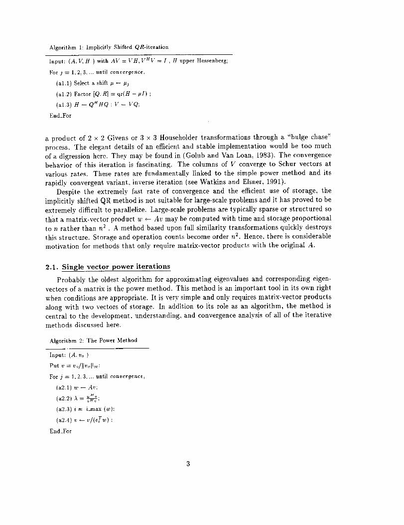
Algorithm 1: Implicitly Shifted QR-iteration
Input.: (A, P; H ) with AV = VH, _/Hv = I , H upper Hessenberg;
For j = 1,2, 3, ... until convergence,
(al.1) Select a shift p _/_j
(al.2) Factor [Q, R] = qr(H -/_I) ;
(al.3) H _ QH HQ ; V _ VQ;
End_For
a product of 2 × 2 Givens or 3 × 3 Householder transformations through a "bulge chase"
process. The elegant details of an efficient and stable implementation would be too much
of a digression here. They may be found in (Golub and Van Loan, 1983). The convergence
behavior of this iteration is fascinating. The columns of V converge to Schur vectors at
various rates. These rates are fundamentally linked to the simple power method and its
rapidly convergent variant, inverse iteration (see Watkins and Elsner, 1991).
Despite the extremely fast rate of convergence and the efficient use of storage, the
implicitly shifted QR method is not suitable for large-scale problems and it has proved to be
extremely difficult to parallelize. Large-scale problems are typically sparse or structured so
that a matrix-vector product w _ Av may be computed with time and storage proportional
to n rather than n 2 . A method based upon full similarity transformations quickly destroys
this structure. Storage and operation counts become order n 2. Hence, there is considerable
motivation for methods that only require matrix-vector products with the original A.
2.1. Single vector power iterations
Probably the oldest algorithm for approximating eigenvalues and corresponding eigen-
vectors of a matrix is the power method. This method is an important tool in its own right
when conditions are appropriate. It is very simple and only requires matrix-vector products
along with two vectors of storage. In addition to its role as an algorithm, the method is
central to the development, understanding, and convergence analysis of all of the iterative
methods discussed here.
Algorithm 2: The Power Method
Input: (A, vo )
Put v = Vo/llVollo_;
For j = 1, 2, 3 .... until convergence,
(a2.1) w -- Av:
why.
(a2.2) ._ = _,
(a2.3) i = i._max (w);
(a2.4) v -- v/(e,_,_,);
End_For
3

At Step(a2.3),i is the index of the element of w with largest absolute value. It is easily
seen that the contents of v after k-steps of this iteration will be the vector
1 Pk p__vk = (eTAkv--------_)Akvo= (eTAkv------_)( Akvo)
for any nonzero scalar Pk. In particular, this iteration may be analyzed as if the vectors had
been scaled by Pk = /_ at each step, with A1 an eigenvalue of A with largest magnitude.
If A is diagonalizable with eigenpairs {(Xj,/_j), I _ j <_ n} and vo has the expansion
b'o : E?-=-I xj"[j in this basis then
1 _ Akxj_/j = _ Xj(/_j/)_t)k,,fj "Akv° = _--_1j=l j=l(3)
If _1 is a simple eigenvalue then
)_))k--* 0, 2<j<n.A:] - -
It follows that vk ---*xl/(eTxl), where i = i__max (Xl), at a linear rate with a convergence
factor of •While the power method is useful, it has two obvious drawbacks. Convergence may be
arbitrarily slow or may not happen at all. Only one eigenvalue and corresponding vector
can be found.
2.2. Spectral transformations
The basic power iteration may be modified to overcome these difficulties. The most fun-
damental modification is to employ a spectral transformation. Spectral transformations
are generally based upon the following:
Let A E C '_x'_ have an eigenvalue _ with corresponding eigenvector x.
1. Let p(r) = 70 + 91r + 72r 2 + ... + %r k- Then p(_) is an eigenvalue of the matrix
p(A) = 3'0I + 3'1A +-72A2 +... + ")'kA k with corresponding eigenvector x (i.e. p(A)x =
xp(A) ).
2. If fir) = _ where p and q are polynomials with q(A) nonsingular, define r(A) =q(,),[q(A)]-lp(A). Then r(A) is an eigenvalue of r(A) with corresponding eigenvector x.
It is often possible to construct a polynomial or rational function ¢(r) such that
I&(li)l <<l¢(,_j)l for l___j_< n, j¢i,
where hi is an eigenvalue of particular interest. This is called a spectral transformation since
the eigenvectors of the transformed matrix ¢(A) remain the same, but the corresponding
eigenvalues _j are transformed to ¢(_j). Applying the power method with ¢(A) in place
of A will then produce the eigenvector q =_ xi corresponding to ,_i at a linear convergence
4

rate with a convergence factor of I¢('xJ) << 1. Once the eigenvector has been found, the¢(A,)
eigenvalue A --- Ai may be calculated directly from a Rayleigh Quotient A = qHAq/qHq.
2.3. Inverse iteration
Spectral transformation can lead to dramatic enhancement of the convergence of the
power method. Polynomial transformations may be applied using only matrix-vector prod-
ucts. Rational transformations require the solution of linear systems with the transformed
matrix as the coefficient matrix. The simplest rational transformation turns out to be
very powerful and is almost exclusively used for this purpose. If p _ a(A) then A - #I is
invertible and a([A - _1]-1) = {I/(A - p) : A E or(A)} . This transformation is very suc-
cessful since eigenvalues near the shift p are transformed to extremal eigenvalues which are
well separated from the other ones while the original extremal eigenvalues are transformed
near the origin. Hence under this transformation the eigenvector q corresponding to the
eigenvalue of A that is closest to p may be readily found and the corresponding eigenvalue
may obtained either through the formula A = 8 + l/p, where _ is the eigenvalue of the
transformed matrix, or it may be calculated directly from a Rayleigh quotient.
Algorithm 3: The Inverse Power Method
Input: (A, t,o,p )
Put v = volllvoll_;
For y = 1, 2, 3.... until convergence,
(a3.1) Solve (A - #I)w -- v;WH_;
(a3.2)), = # + _;
(a3.3) i---- i._max (w);
(a3.4) v- v/(eTu,) ;
End_For
Observe that the formula for A at Step (a3.2) is equivalent to forming A = (wHAw)/(wHw)
so an additional matrix vector product is not necessary to obtain the Rayleigh quotient esti-
mate. The analysis of convergence remains entirely in tact. This iteration converges linearly
with the convergence factor
IA2- #I'
where the eigenvalues of A have been re-indexed so that ]A] - #l < IA=- #I _<IA3- #I <_•-. -< IA_ - #1" Hence, the convergence becomes faster as # gets closer to AI.
This result is encouraging but still leaves us wondering how to select the shift # to be
close to the unknown eigenvalue we are trying to compute. In many applications the choice
is apparent from the requirements of the problem. It is also possible to change the shift
at each iteration at the expense of a new matrix factorization at each step. An obvious
choice would be to replace the shift with the current Rayleigh quotient estimate. This
method, called Rayleigh Quotient (RQ) iteration, has very impressive convergence rates
indeed. Rayleigh Quotient Iteration converges at a quadratic rate in general and at a cubic

rate on Hermitian problems. For a more detailed discussion of the eigenvalue problem and
basic algorithms see (Golub and Van Loan, 1983, Stewart, 1973, and Wilkinson, 1965).
3. Krylov Subspaces and Projection Methods
Although the rate of convergence can be improved to an acceptable level through spec-
tral transformations, power iterations are only able to find one eigenvector at a time. If
more vectors are sought, then various deflation techniques (such as orthogonalizing against
previously converged eigenvectors) and shift strategies must be introduced. One alternative
is to introduce a block form of the simple power method which is often called subspace iter-
ation. This important class of algorithms has been developed and investigated in (Stewart,
1973). Several software efforts have been based upon this approach (Bai and Stewart, 1992,
Duff and Scott, 1993, and Stewart and Jennings, 1992). However, there is another class
of algorithms called Krylov subspace projection methods that are based upon the intricate
structure of the sequence of vectors naturally produced by the power method.
An examination of the behavior of the power sequence as exposed in equation (3) hints
that the successive vectors produced by a power iteration may contain considerable infor-
mation along eigenvector directions corresponding to eigenvalues other than the one with
largest magnitude. The expansion coefficients of the vectors in the power sequence evolve
in a very structured way. Therefore, linear combinations of the these vectors might well be
devised to expose additional eigenvectors. A single vector power iteration simply ignores
this additional information, but more sophisticated techniques may be employed to extractit.
If one hopes to obtain additional information through various linear combinations of the
power sequence, it is natural to formally consider the Krylov subspace
Kk(A, vl) = Span {Vl, Avl, A2vl,..., Ak-lvl}
and to attempt to formulate the best possible approximations to eigenvectors from this
subspace.
It is reasonable to construct approximate eigenpairs from this subspace by imposing a
Galerkin condition: A vector x E h:k(A, vl) is called a Ritz vector with corresponding Ritzvalue 0 if the Galerkin condition
< w, Ax - xO >= 0, for all w E gk(A, Vl)
is satisfied. There are some immediate consequences of this definition: Let W be a matrix
whose columns form an orthonormal basis for Kk ----K:k(A, vl). Let P = WW H denote the
related orthogonal projector onto K;k and define ft = 7)A'P = WBW H, where B =_WH AW.
It can be shown that
Lemma 3 For the quantities defined above:
1. (x, 0) is a Ritz-pair if and only if x = Wy with By = yO .
2. [l(!- P)AW[[ = II(A- A)W[I _< [I(A- M)WI[
.for all M E C '_xn such that MICA C ICk.

3. TheRitz-pairs(x, O) and the minimum value of [](I - P)AWI[ are independent of the
choice of orthonormal basis W.
Item (1) follows immediately from the Galerkin condition since it implies that 0 = WH(AWy -
I4"yO) = By - yO. Item (2)is easily shown using invariance of I1" II under unitary transfor-
mations. Item (3) follows from the fact that V is an orthonormal basis for KYk if and only if
V = WQ for some k x k unitary matrix Q. With this change of basis A = VHV H, where
H = VHAV = QHBQ. Since H is unitarily similar to B, the Ritz-values remain the same
and the Ritz-vectors are of the form x = Wy = V_), where _ = QHy.
These facts are actually valid for any k dimensional subspace S in place of K;k. The
following properties are consequences of the fact that every w E KYk is of the form w =
¢(A)vl for some polynomial ¢ of degree less than k.
Lemma 4 For the quantities defined above:
1. If q is a polynomial of degree less than k then
q(A)vl = q(A)vl = Wq(B)zl,
where vl = _/Vzl, and if the degree of q is k then
Pq(A)vl = q(A)Vl.
2. ff _( )_) = det(,_I - B) is the characteristic polynomial of B then b(,4) = 0 and
liP(A) v, II <- Nq(A )v_ IIIor all monic polynomials of degree k.
3. If y is any vector in C k then AWy - WBy = 7/)(A)vl for some scalar 7.
4. If (x, O) is any Ritz-pair for A with respect to ]Ck then
Ax - xO = 715(A)Vl
for some scalar 7.
This discussion follows the treatment given by Saad in (Saad, 1992) and in his earlier
papers. While these facts may seem esoteric, they have important algorithmic consequences.
First, it should be noted that /C_ is an invariant subspace for A if and only if Vl = Vy,
where AV = VR with vHv = Ik and R is k x k upper triangular. Also,/Ck is an invariant
subspace for A if vl = Xy, where X E C '_xk and AX = XA with A diagonal. This follows
from items (2) and (3) since there is a k-degree monic polynomial q such that q(R) = 0 and
hence 11ih(A)vlH _< Hq(A)vlH = I]Yq(R)y]l = 0. (A similar argument holds when vl = Xy).
Secondly, there is some algorithmic motivation to seek a convenient orthonormal basis
V = WQ that will provide a means to successively construct these basis vectors. It is
possible to construct a k × k unitary Q using standard Householder transformations such that
vl = Vel and H = QHBQ is upper Hessenberg with non-negative subdiagonal elements.
It is also possible to show using item (3) that in this basis,
AV = VH + fe T, where f=7[_(A)vl

and vHf = 0 follows from the Galerkin condition.
The first observation shows that if it is possible to obtain a Vl as a linear combination
of k eigenvectors of A then f = 0 and V is an orthonormal basis for an invariant subspace
of A, and that the Ritz values or(H) C a(A) and corresponding Ritz vectors are eigenpairs
for A. The second observation leads to the Lanczos/Arnoldi process (Arnoldi, 1951 and
Lanczos, 1950).
4. The Arnoldi Factorization
Definition : If A E C n×'_ then a relation of the form
Al/'k = VkHk + fke T,
where 1/_: E C nxk has orthonormal columns, vHfk = 0 and Hk E C kxk is upper Hessenberg
with non-negative subdiagonal elements is called a k-step Arnoldi Factorization of A. If A
is Hermitian then Hk is real, symmetric and tridiagonal and the relation is called a k-stepLanczos Factorization of A. The columns of Vk are referred to as the Arnoldi vectors or
Lanczos vectors respectively.
The development of this factorization has been purely through the consequences of the
orthogonal projection imposed by the Galerkin conditions. A more straightforward but less
illuminating derivation is to simply truncate the reduction of A to Hessenberg form that
precedes the implicitly shifted QR-iteration by equating the first k columns on both sides
of the complete reduction AV = VH. An alternative way to write this factorization is
(Hk) where/3k=,,fkNandvk+l=__kf kAt_ = (Vk, Vk+l) _keT
This factorization may be used to obtain approximate solutions to a linear system Ax = b
if b = Vlflo. The purpose here is to investigate the use of this factorization to obtain ap-
proximate eigenvalues and eigenvectors. The discussion of the previous section implies that
Ritz pairs satisfying the Galerkin condition are immediately available from the eigenpairs
of the small projected matrix H.
If Hky = yO then the vector x = _y satisfies
[lAx - xOII = II(AVk - VkHk)ytl = 1,2keTy[.
The number lflkeTy] is called the Ritz estimate for this the Ritz pair (x, 0) as an approxi-
mate eigenpair for A. Observe that if (x, 0) is a Ritz pair then
0 = yHHky = (Vky)HA(Vky) = xHAx
is a Rayleigh Quotient (assuming IlyH = 1) and the associated Rayleigh Quotient residual
r( x ) = Ax - xO satisfies
= fZkekyt.IIr(x)ll z
When A is Hermitian, this relation may be used to provide computable rigorous bounds on
the accuracy of the eigenvalues of H as approximations to eigenvalues of A; see (Parlett,
8
1980).When A is non-Hermitian the possibility of non-normality precludes such boundsand one can only say that the RQ-residual is smallif ]_keTyl is small. However, in either
case, if fk = 0 these the Ritz pairs become exact eigenpairs of A.
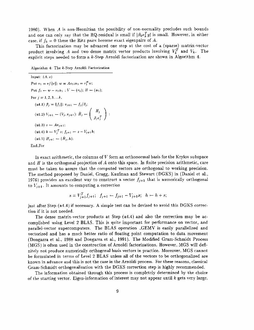
This factorization may be advanced one step at the cost of a (sparse) matrix-vector
product involving A and two dense matrix vector products involving VT and 1/)¢. The
explicit steps needed to form a k-Step Arnoldi factorization are shown in Algorithm 4.
Algorithm 4: The k-Step Arnoldi Factorization
Input: {A, v)
Put _,_= ,,/11,'11;,-,-'= Av,;o_, = ,,_,,,;
Put ]'1 -- w- vial ; V -- (vl); H -- (_1);
For j = 1,2, 3, ...k,
(a4A) _j = IIf.,ll; v,+, - L/_J;
(_.4.2)v_+_ - (v_, v,+,); H, -- _-,_T ;
(a4.3) z _ Av3+l;
(a4.4) h _ V3T z; f_+l _ z -- Ii_+lh;
(a4.S) H_+I -- (/:/3, h);
End_For
In exact arithmetic, the columns of V form an orthonormal basis for the Krylov subspace
and H is the orthogonal projection of A onto this space. In finite precision arithmetic, care
must be taken to assure that the computed vectors are orthogonal to working precision.
The method proposed by Daniel, Gragg, Kaufman and Stewart (DGKS) in (Daniel et al.,
1976) provides an excellent way to construct a vector fj+l that is numerically orthogonal
to t_+l. It amounts to computing a correction
IT8 = _'j+lfj+l; fj+l +-- fj+l -- Vj+I'.q; h +- h + 8;
just after Step (a4.4) if necessary. A simple test can be devised to avoid this DGKS correc-
tion if it is not needed.
The dense matrix-vector products at Step (a4.4) and also the correction may be ac-
complished using Level 2 BLAS. This is quite important for performance on vector, and
parallel-vector supercomputers. The BLAS operation _GEMV is easily parallelized and
vectorized and has a much better ratio of floating point computation to data movement
(Dongarra et al., 1988 and Dongarra et al., 1991). The Modified Gram-Schmidt Process
(MGS) is often used in the construction of Arnoldi factorizations. However, MGS will defi-
nitely not produce numerically orthogonal basis vectors in practice. Moreover, MGS cannotbe formulated in terms of Level 2 BLAS unless all of the vectors to be orthogonalized are
known in advance and this is not the case in the Arnoldi process. For these reasons, classical
Gram-Schmidt orthogonalization with the DGKS correction step is highly recommended.
The information obtained through this process is completely determined by the choice
of the starting vector. Eigen-information of interest may not appear until k gets very large.
9

In this caseit becomesintractableto maintainnumericalorthogonalityof the basisvectorsl,_. Moreover,extensivestoragewill berequiredandrepeatedlyfinding the eigensystemofH will become prohibitive at a cost of O(k 3) flops.
Failure to maintain orthogonality leads to several numerical difficulties. In a certain
sense, the computation (or approximation) of the projection indicated at Step (a4.4) in a
way that overcomes these difficulties has been the main source of research activity in these
Krylov subspace projection methods. The computational difficulty stems from the fact that
[[fk[[ = 0 if and only if the columns of Vk span an invariant subspace of A. When Vk "nearly"
spans such a subspace [[fk[[ will be small. Typically, in this situation, a loss of significant
digits will take place at Step (a4.4) through numerical cancellation unless special care is
taken (i.e., use of the DGKS correction).
It is desirable for [Ifk[[ to become small because this indicates that the eigenvalues of
H are accurate approximations to the eigenvalues of A. However, this "convergence" will
indicate a probable loss of numerical orthogonality in V. Moreover, if subsequent Arnoldi
vectors are not forced to be orthogonal to the converged ones then components along these
directions re-enter the basis via round-off effects and quickly cause a spurious copy of the
previously computed eigenvalue to appear repeatedly in the spectrum of the projected
matrix H. The identification of this phenomenon in the symmetric case and the first rigorous
numerical treatment is due to Paige (1971). There have been several approaches to overcome
this problem in the symmetric case. They include: (1) complete re-orthogonalization, which
may be accomplished through maintaining V in product Householder form (Walker, 1988)
or through the Modified Gram-Schmidt processes with re-orthogonalization (Daniel et al.,
1976). (2) Selective re-orthogonalization, which has been proposed by Parlett and has been
heavily researched by him and his students. Most notably, the theses and subsequent papers
and computer codes of Scott and of Simon have developed this idea (Parlett and Scott, 1979,
Parlett, 1980, and Simon, 1984). (3) No re-orthogonalization, which has been developed
by Cullum and her colleagues. This last option introduces the almost certain possibility
of introducing spurious eigenvalues. Various techniques have been developed to detect and
deal with the presence of spurious eigenvalues (Cullum, 1978 and Cullum and Willoughby,1981).
The appearance of spurious eigenvalues may be avoided through complete orthogonal-
ization of the Arnoldi (or Lanczos) vectors using the DGKS correction. Computational cost
has been cited as the reason for not employing this option. However, the cost will be rea-
sonable if one is able to fix k at a modest size and then update the starting vector vl = lZ_el
while repeatedly doing k-Arnoldi steps. This approach was introduced in (Karush, 1951)
and developed further by (Cullum and Donath, 1974) for the symmetric case. Saad (1980,
1984, and 1992) has developed explicit restarting for the nonsymmetric case. Restarting hasproven to have important consequences for the development of numerical software based
upon Arnoldi's method and this will be explored in the following section.
5. Restarting the Arnoldi Method
An unfortunate aspect of the Lanczos/Arnoldi process is that one cannot know in ad-
vance how many steps will be required before eigenvalues of interest are well approximated
by Ritz values. This is particularly true when the problem has a wide range of eigenvalues
10
but the eigenvalues of interest are clustered. For example, in computational chemistry,
problems are usually symmetric and positive definite and there is a wide range of eigenval-
ues varying over many orders of magnitude. Only the smallest eigenvalues are physically
interesting and they are typically clustered at the low end of the spectrum. Shift and invert
is usually not an option because of fill in from the factorizations. Without a spectral trans-
formation, many Lanczos steps are required to obtain the smallest eigenvalues. In order to
recover eigenvectors, one is obliged to store all of the Lanczos basis vectors (usually on a
peripheral device) and to solve very large tridiagonal eigenvalue subproblems at each step.
In the Arnoldi process that is used in the non-Hermitian case, not only do the basis vectors
have to be stored, but the cost of the Hessenberg eigenvalue subproblem is O(k 3) at the
k-th step.
5.1. Explicit restarting
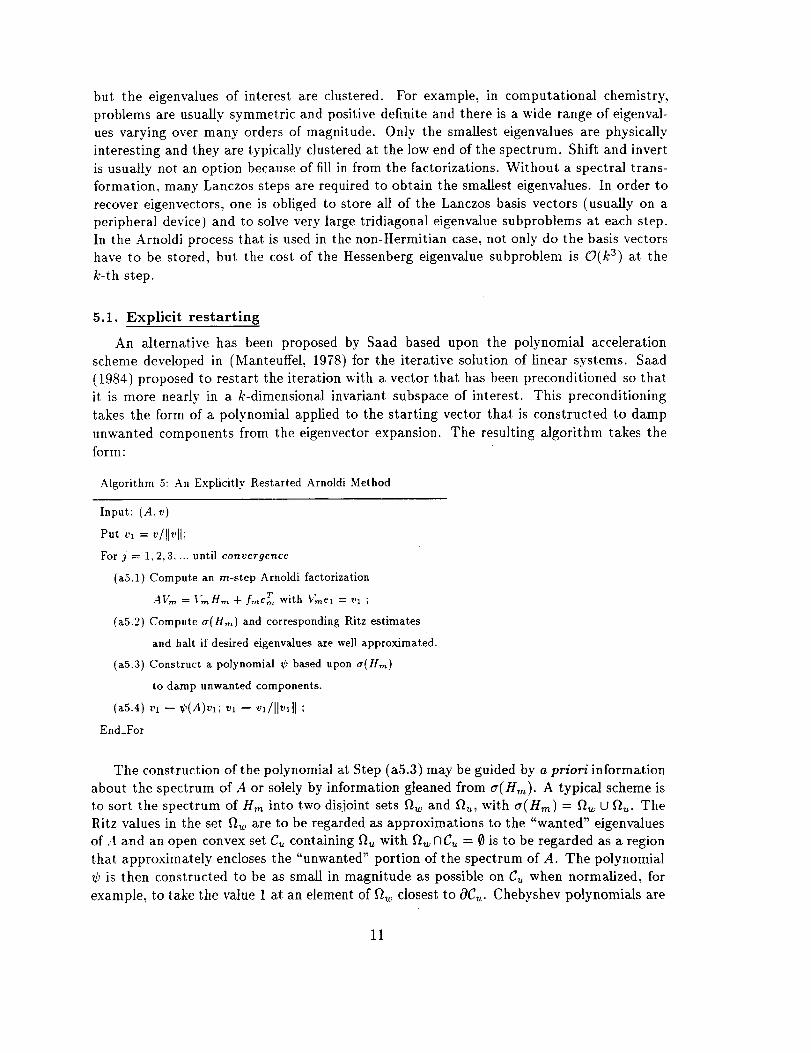
An alternative has been proposed by Saad based upon the polynomial acceleration
scheme developed in (Manteuffel, 1978) for the iterative solution of linear systems. Saad
(1984) proposed to restart the iteration with a vector that has been preconditioned so that
it is more nearly in a k-dimensional invariant subspace of interest. This preconditioning
takes the form of a polynomial applied to the starting vector that is constructed to damp
unwanted components from the eigenvector expansion. The resulting algorithm takes the
form:
Algorithm 5: An Explicitly Restarted Arnoldi Method
Input: (A,v)
Put vl = v/[[vH;
For i = 1,2,3 .... until convergence
(a5.1) Compute an m-step Arnoldi factorization
AVm = _"_Hm + fme_ with i"_el = vl ;
(a5.2) Compute a(Hm) and corresponding Ritz estimates
and halt if desired eigenvalues are well approximated.
(a5.3) Construct a polynomial _ based upon a(Hm)
to damp unwanted components.
(a5.4) v, -- e'(A)v,; v, -- v,/llv, II ;
End_For
The construction of the polynomial at Step (a_5.3) may be guided by a priori information
about the spectrum of A or solely by information gleaned from a(Hm). A typical scheme is
to sort the spectrum of Hm into two disjoint sets f_w and flu, with a(Hm) = f_w U flu. The
Ritz values in the set f_w are to be regarded as approximations to the "wanted" eigenvalues
of A and an open convex set Cu containing flu with _twAC u = 0 is to be regarded as a region
that appro_mately encloses the "unwanted" portion of the spectrum of A. The polynomial
is then constructed to be as small in magnitude as possible on C_ when normalized, for
example, to take the value 1 at an element of ftw closest to OCt. Chebyshev polynomials are
11

appropriatewhenCu is taken to be an ellipse and this was the original proposal of Saad when
he adapted the Manteuffel idea to eigenvalue calculations. Another possibility explored by
Saad has been to take Cu to be the convex hull of _tu and to construct the polynomial _b that
best approximates 0 on this set in the least squares sense. Both of these are based upon
well-known theory of polynomial approximation. The problem of constructing an optimal
ellipse for this problem has been studied by Chatelin and Ho. The reader is referred to
(Chatelin and Ho, 1990) for details of constructing these polynomials.
The reasoning behind this type of algorithm is that that if vl is a linear combination of
precisely k eigenvectors of A then Arnoldi factorization terminates in k steps (i.e., fk = 0).
The columns of IJ)¢ will form an orthonormal basis for the invariant subspace spanned by
those eigenvectors, and the Ritz values a(Hk) will be the corresponding eigenvalues of A.
The update of the starting vector vl is designed to enhance the components of this vector
in the directions of the wanted eigenvectors and damp its components in the unwanted
directions. This effect is achieved at Step (a5.4) since
- fit'l ---- Z Xj"_j _ ¢(A)th = xj_'(_j)73.
j=l j=l
If the same polynomial were appLied each time, then after M iterations, the j-th original
expansion coefficient would be essentially attenuated by a factor
¢(Aj) M
where the eigenvalues have been ordered according decreasing values t_b(2j))l. The eigen-
values inside the region Cu become less and less significant as the iteration proceeds. Hence,
the wanted eigenvalues are approximated increasingly well as the iteration proceeds.
Another restarting strategy proposed by Saad is to replace the starting vector with a
linear combination of Ritz vectors corresponding to wanted Ritz values. If the eigenvalues
and corresponding vectors are re-indexed so that the first k are wanted and (&j, Oj) is the
the Ritz pair approximating the eigenpair (xj, ,_j) then
k
(4)j----1
is taken as the new starting vector. Again, the motivation here is that the Arnoldi residual
fk would vanish if these k Ritz vectors were actually eigenvectors of A and the Ritz vectors
are the best available approximations to these eigenvectors. A heuristic choice for the
coefficients Fj has also been suggested by Saad (1980). It is to weight the j-th Ritz vector
with the value of its Ritz estimate and then normalize so that the new starting vector
has norm 1. This has the effect of favoring the Ritz vectors that have least converged.
Additional aspects of explicit restarting are developed thoroughly in Chapter VII of (Saad,
1992). In any case, this restarting mechanism is actually polynomial restarting in disguise.
Since &j E ]_m(A, vl) implies _j = Cj(A)vl for some polynomial Cj the formula for v + in
(4) is of the formk
v + ,--- ¢(A)v, - _ ?jCj(A)v,. (5)j=l
12

The technique just described is referred to as explicit (polynomial) restarting. When
Chebyshev polynomials are used it is called an Arnoldi-Chebyshev method. The cost in
terms of matrix-vector products w +- Av is M * (m + deg(_)) for M major iterations. The
cost of the arithmetic in the Arnoldi factorization is M * (2n * m 2 + O(m3)) Flops (floating
point operations). Tradeoffs must be made in terms of cost of the Arnoldi factorization vs.
cost of the matrix-vector products Av and also in terms of storage (nm + O(m2)).
5.2. Implicit restarting
There is another approach to restarting that offers a more efficient and numerically
stable formulation. This approach, called implicit restarting, is a technique for combining
the implicitly shifted QR mechanism with a k-step Arnoldi or Lanczos factorization to
obtain a truncated form of the implicitly shifted QR-iteration. The numerical difficulties
and storage problems normally associated with Arnoldi and Lanczos processes are avoided.
The algorithm is capable of computing a few (k) eigenvalues with user specified features such
as largest real part or largest magnitude using 2nk + O(k 2) storage. No auxiliary storage
is required. The computed Schur basis vectors for the desired k-dimensional eigenspace are
numerically orthogonal to working precision. This method is well suited to the developmentof mathematical software and this will be discussed in Section 7.
Implicit restarting provides a means to extract interesting information from very large
Krylov subspaces while avoiding the storage and numerical difficulties associated with the
standard approach. It does this by continually compressing the interesting information into
a fixed size k-dimensional subspace. This is accomplished through the implicitly shifted QR
mechanism. An Arnoldi factorization of length m = k + p
AVm = I_H,,_ + free T, (6)
is compressed to a factorization of length k that retains the eigen-information of interest.
This is accomplished using QR steps to apply p shifts implicitly. The first stage of this shift
process results in
AV + -+ + , T=Pm Hm + fmemQ, (7)
where _ = VmQ, H + = QT HmQ, and Q = Q1Q2 " " "Qp, with Qj the orthogonal matrix
associated with the shift #j. It may be shown that the first k - 1 entries of the vector eTQ
are zero (i.e. eTQ = (ae T,_I T) ). Equating the first k columns on both sides yields an
updated k-step Arnoldi factorization
AV + V+ rr+ + T= k-k +f_ek, (8)
with an updated residual of the form f+ = V_+pek+l_k + fk+pa. Using this as a starting
point it is possible to apply p additional steps of the Arnoldi process to return to the original
m-step form.
Each of these shift cycles results in the implicit application of a polynomial in A of
degree p to the starting vector.
P
vl "-- g,(A)vl with _b(A) = I-[(A - #j).1
13

The roots of this polynomial are the shifts used in the QR process and these may be
selected to filter unwanted information from the starting vector and hence from the Arnoldi
factorization. Full details may be found in (Sorensen, 1992). The basic iteration is given
here in Algorithm 6 and the diagrams in Figures 1-3 describe how this iteration proceeds
schematically. In Algorithm 6 and in the discussion below, the notation M(l:n,]:k ) denotes
the leading n × k submatrix of M.
J | : :: |
:i
;:}:i I
s TFigure h Representation of I_.+pl/_+p + J'k+p k÷p"
uonzeTos.
J •
Shaded regions denote
iiiiiiiiiiiiii_i:(_iiiii!
iiiii!_i_i_I¸¸:¸i....
?i!i_iil :ii_iiiii_i!i_ii|i¸ _i_ii_:i!ii!!i!_ i:ii!_?
iiiiiiiiii_::iii
iiiiiiiiiii;_$:_i;_i;!iiilm•
Figure 2: I'_+;,QQT H;c+,,Q r+ .f;:+pe,_+pQ after p implicitly shifted QR steps.
÷
_k_ k
Figure 3: Leading k columns l',llt, + .[j,e[" form a length k Arno[di factor-
ization after discarding the la.st p columns.
14

Observethat if m = n then f = 0 and this iteration is precisely the same as the Implicitly
Shifted QR iteration. Even for m < n, the first k columns of V and the Hessenberg
submatrix H(l:k,l:k) are mathematically equivalent to the matrices that would appear in the
full Implicitly Shifted QR iteration using the same shifts/zj. In this sense, the Implicitly
Restarted Arnoldi method may be viewed as a truncation of the Implicitly Shifted QR
iteration. The fundamental difference is that the standard Implicitly Shifted QR iteration
selects shifts to drive subdiagonal elements of H to zero from the bottom up while the
shift selection in the Implicitly Restarted Arnoldi method is made to drive subdiagonal
elements of H to zero from the top down. Important implementation details concerning the
deflation (setting to zero) of subdiagonal elements of H and the purging of unwanted but
converged Ritz values are beyond the scope of this discussion. However, these details are
extremely important to the success of this iteration in difficult cases. Complete details of
these numerical refinements may be found in (Lehoucq, 1995 and Lehoucq and Sorensen,
1994).
Algorithm 6: An Implicitly Restarted Arnoldi Method
Input: (A, V, H, f) with AVm = _Hm + free T,
(an m-Step Arnoldi Factorization);
For £ = 1, 2, 3.... until convergence
(a6.2) Compute a(Hm) and select set of p shifts/zl, it2, ...p.v
based upon a(Hm) or perhaps other information;
(a6.3) qT Tera;
(a6.4) For ) = 1, 2 .... ,p,
Factor [Q3, Rj] = qr(Hm -/_jI);
Hm -- QH Hm Q3 ; vm -- vm Q3;
q _ qHQ;;
End_For
(a6.5) fk _ vk+lflk + freak; Vk _ Vm(a:_3:k); Hk _ H,n(l:k,l:k);
(a6.6) Beginning with the k-step Arnoldi factorization
At"k = VkHk + fke T,
apply p additional steps of the Arnoldi process
to obtain a new m-step Arnoldi factorization
e TA i,_ = Vm H,_ + f,_ m.
End_For
The above iteration can be used to apply any known polynomial restart. If the roots
of the polynomial are not known there is an alternative implementation that only requires
one to compute ql = zp(H)el, where _b is the desired degree p polynomial. A sequence of
Householder transformations may developed to form a unitary matrix Q such that Qel = ql
and H _ QHHQ is upper Hessenberg. The details which follow standard developments for
the Implicitly Shifted QR iteration will be omitted here.
15

A shift selection strategy that has proved successful in practice is called the "Exact Shift
Strategy". In this strategy, one computes a(H) and sorts this into two disjoint sets f_ and
_. The k Ritz values in the set _,_ are regarded as approximations to the "wanted"
eigenvalues of A, and the p Ritz values in the set f2_ are taken as the shifts pj. An
interesting consequence (in exact arithmetic) is that after Step (a6.4) above, the spectrum
of Hk in Step (a6.5) is a(Hk) = _ and the updated, starting vector vl is a particular linearcombination of the k Ritz vectors associated with these Ritz values. In other words, the
implicit restarting scheme with exact shifts provides a specific selection of the coefficients 7j
in Eq. (4) and this implicit scheme costs p rather than the k + p matrix-vector products the
explicit scheme would require. Thus the exact shift strategy can be viewed both as a means
to damp unwanted components from the starting vector and also as directly forcing the
starting vector to be a linear combination of wanted eigenvectors. The exact shift strategy
has two additional interesting theoretical properties.
Lemma 5 If H is unreduced and diagonalizable then:
1. The polynomial ¢ in (5) satisfies ¢(A) = ¢(A)p(A),
where _, is the ezaet .shift polynomial and p is some
polynomial of degree at most k - 1.
2. The updated Krylov subspace generated by the new
starting vector satisfies
ICm(a, v+) = Span{_a, _,..., _k, AY:j, A2_:j, .. . , AP_j}
for j= 1,2,-..,k.
The first property _(_) = _(_)p()_) indicates that the linear combination selected by theexact shift scheme is somehow minimal while the second property indicates that each of the
subspaces ICp(A,_j) C ICm(A, v+) so that each sequence of "wanted" Ritz vectors is rep-
resented equally in the updated subspace. The first property was established in (Lehoucq,
1995) along with an extensive analysis of the numerical properties of impficit restarting. The
surprising second property was established in (Morgan, 1996), along with some compelling
numerical results indicating superior performance of implicit over explicit restarting.
6. The Generalized Eigenvalue Problem
A typical source of large-scale eigenproblems is through a discrete form of a contin-
uous problem. The resulting finite-dimensional problems become large due to accuracy
requirements and spatial dimensionality. Typically this takes the form
/:u = uA in fl, (9)
u satisfies /3 on 0_,
where £ is some linear differential operator. A number of techniques may be used to
discretize £:. The finite element method provides an elegant discretization. If }4/is a space
of functions in which the solution to (9) may be found and }_Y_C }4" is an n-dimensional
16

subspacewith basisfunctions{¢j} thenan approximatesolution u,_ is expanded in theform
n
j=l
A variational or a GMerkin principle is applied depending on whether or not/2 is self-adjoint,
leading to a weak form of (9)
A(v,u) = ,_ < v,u >, (10)
where A(v, u) is a bilinear form. Substituting the expanded form of u = u_ and requiring
(10) to hold for each trim function v = ¢i gives a set of algebraic equations
j=l j=l
where < -,- > is an inner product in 14,'_. This leads to the following systems of equations
_-_.A(¢i,¢j)_j = A _-'_ < ¢i,¢j > (j, (11)j=l j=l
for 1 < i < n. We may rewrite (11) and obtain the matrix equation
Ax = ,_Mx,
where
di,j = A(Oi,¢j), Mi,j =< ¢i,¢j >, x T = [_1,..-,_n] T,
for 1 _< i,j _< n. Typically the basis functions are chosen so that few entries in a row of
A or M are nonzero. In structures problems A is called the "stiffness" matrix and M is
called the "mass" matrix. In chemistry and physics M is often referred to as the "overlap"
matrix. A nice feature of this approach to discretization is that if the basis functions Cj all
individually satisfy B on 0f_ then the boundary conditions are naturally incorporated into
the discrete problem. Moreover, in the self-adjoint case, the Rayleigh principle is preserved
from the continuous to the discrete problem. In particular, since Ritz values are Rayleigh
quotients, this assures the smallest Ritz value is greater than the smallest eigenvalue of the
original problem.Thus, it is natural for large-scale eigenproblems to arise as generalized rather than
standard problems. If/2 is self-adjoint the discrete problems are symmetric or Hermitian
and if not the matrix A is nonsymmetric but the matrix M is symmetric and at. least
positive semi-definite. There are a number of ways to convert the generalized problem tostandard form. There is always motivation to preserve symmetry when it is present.
If M is positive definite then there exists a factorization M = LL T, and the eigenvalues
of ,4 =- L-1AL -T are the eigenvalues of (A,M), and the eigenvectors are obtained bysolving LTx = ,_, where 37is an eigenvector of A. This standard transformation is fine if one
wants the eigenvalues of largest magnitude and it preserves symmetry if A is symmetric.However, when M is ill-conditioned this can be a dangerous transformation leading to
17
numericaldifficulties. Sincea matrix factorizationwill haveto bedoneanyway,onemayaswell formulatea spectraltransformation.
6.1. Structure of the spectral transformation
A convenient way to provide a spectral transformation is to note that
Ax= AMx _ (A-IIM)x=(A-p)Mx
Thus1
(A - #M)-IMx = xO, where 0 = __---[--_.
If A is symmetric then one can maintain symmetry in the Arnoldi/Lanczos process by
taking the inner product to be< x,y >= xTMy.
It is easy to verify that the operator (A - #M)-IM is symmetric with respect to this inner
product if A is symmetric. In the Arnoldi/Lanczos process the matrix-vector product wAv is replaced by w ,- (A-pM)-IMv and the step h _ vT f is replaced by h _ VT(M f).
If A is symmetric then the matrix H is symmetric and tridiagonal. Moreover, this process
is well defined even when M is singular and this can have important consequences even if
A is nonsymmetric. We shall refer to this process as the M-Arnoldi process.
If M is singular then the operator S =- (A - I_M)-IM has a nontrivial null space and
the bilinear function < x, y >= xTMy is a semi-inner product and [[Xl[M --< x, y >1/2 is a
semi-norm. Since (A- #M) is assumed to be nonsingular, A/" -Null(S) =Null(M). Vectors
in A" are generalized eigenvectors corresponding to infinite eigenvalues. Typically, one is
only interested in the finite eigenvalues of (A, M) and these will correspond to the nonzero
eigenvalues of S. The invariant subspace corresponding to these nonzero eigenvalues is
easily corrupted by components of vectors from 2¢" during the Arnoldi process. However,
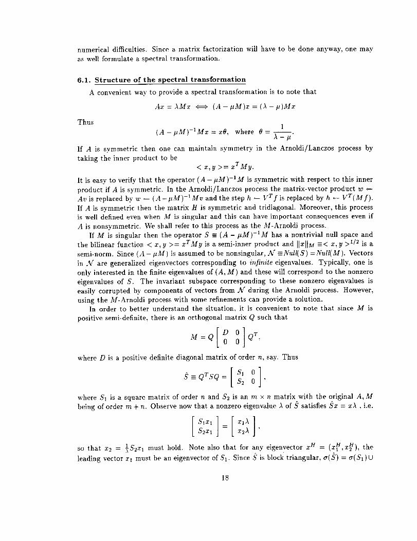
using the M-Arnoldi process with some refinements can provide a solution.In order to better understand the situation, it is convenient to note that since M is
positive semi-definite, there is an orthogonal matrix Q such that
M=Q[ DO O]QT,o
where D is a positive definite diagonal matrix of order n, say. Thus
S-QTSQ= [ S' ° 1$2 o '
where $1 is a square matrix of order n and $2 is an ra × n matrix with the original A, M
being of order ra + n. Observe now that a nonzero eigenvalue A of S satisfies Sx = xA , i.e.
SlXl = x2A ]'
so that x2 = _$2Xl must hold. Note also that for an)' eigenvector x H = (x_,xH), the
leading vector xl must be an eigenvector of $1. Since S is block triangular, a(S) = a(S1)U
18

a(0m). Assuming S_ has full rank, it follows that if $1 has a zero eigenvalue then there is no
corresponding eigenvector (since $2xl = 0 would be implied). Thus if zero is an eigenvalue
of S1 with algebraic multiplicity mo then zero is an eigenvalue of S of algebraic multiplicity
m + mo and with geometric multiplicity m. Of course, since, S is similar to S all of these
statements hold for S as well.
6.2. Eigenvector/null-space purification
With these observations in hand, it is possible to see the virtue of using M-Arnoldi on
S. After k-steps of M-Arnoldi,
SV = VH + fe T with VTMV = Ik, vTMf = O.
Introducing the similarity transformation Q gives
^rT TSI ?=('H+ fe T with t' Q MQV=Ik,VTQ TMQ]=O,
where V = QTv and .f = QTf. Partitioning 1?T = (vaTv f) and .fT = (fT, ff) consistent
with the blocking of S gives
sltq = t]H + with V(DV, = Ik,V rDfl = 0.
Moreover, the side condition $2V1 = V2H + f2e [ holds, so that in exact arithmetic a zero
eigenvalue should not appear as a converged Ritz value of H. This argument shows that
M-Arnoldi on S is at the same time doing D-Arnoldi on $1 while avoiding convergence to
zero eigenvalues.
Round-off error due to finite precision arithmetic will cloud the situation, as usual. It
is clear that the goal is to prevent components in Af from corrupting the vectors V. Thus,
to begin, the starting vector vl should be of the form vl = Sv. If a final approximate
eigenvector x has components in A f they may be purged by replacing x _ Sx and then
normalizing. To see the effect of this, note that if x = Q x2Xa then Sx = Q $2xl '
0 ] will have been purged. Thisand all components in N" which are of the form Q p
final application of S may be done implicitly in two ways. One is to note that if x = VyTwith IIy = yO then Sx = VHy + fe_y = xO + fe k y, and this is the correction suggested
by (Nour-Omid et al., 1987). Another recent suggestion due to Meerbergen and Spence
is to use implicit restarting with a zero shift (Meerbergen and Spence, 199.5). Recall that
implicit restarting with g zero shifts is equivalent to starting the M-Arnoldi process with a
starting vector of Sevl and all the resulting Ritz vectors will be multiplied by S _ as well.
After applying the implicit shifts to H, the leading submatrix of order k- g will provide the
updated Ritz values. No additional explicit matrix-vector products with S are required.
The ability to apply _ zero shifts (i.e., to multiply by S e implicitly) is very important
when $1 has zero eigenvalues. If ocxXl = 0 then
[,,0][xi]:[0]$2 0 x2 $2zl EAr.
19

Thus to completely eradicate components from .M one must multiply by S _, where g is equal
to the dimension of the largest Jordan block corresponding to a zero eigenvalue of $1.
Spectral transformations were studied extensively by Ericsson and Ruhe (1980) and the
first eigenvector purification strategy was developed in (Nour-Omid et al., 1987). Shift and
invert techniques play an essential role in the block Lanczos code developed by Grimes,
Lewis, and Simon. The many nuances of this technique in practical applications are dis-
cussed thoroughly in (Grimes et al., 1994). The development presented here and the eigen-
vector purification through implicit restarting is due to Meerbergen and Spence (1995).
6.3. An example
This discussion is illustrated with the following example.
[ K C] and M= [ I O]A= cT 0 0 0 '
with A an order 325 matrix approximation to a convection-diffusion operator and C a
structured random matrix. This example was chosen because it has the block structure of
a typical steady-state Navier-Stokes linear stability analysis; see (Meerbergen and Spence,
199.5). The following MATLAB code was used to generate the example:
rand( 'seed' ,0) ;
n = 225;m=I00;
K = lapc(n,100);
C = [rand(m,m) ; zeros(n-m,m)];
S = [eye(n) zeros(n,m) ; zeros(m,n) zeros(m,m)];
A = [K C ; C' zeros(m,m)];
mu = 7.0;
S = (A - mu*M)\M;
The matrices K, C, M, A correspond to the matrices in the equations above. The function
lapc computes a finite difference approximation to Au + pu:: on a 15 × 15 regular grid in
the unit square with p = 100. Any matrix pencil (A, M) with this block structure (assuming
C has full rank and A - pM is nonsingular) will produce an S of the form
[000]S = 0 Sn 0 ,
$31 $32 0
with the upper-left zero block of order m and with $22 nonsingular and order n - m. From
the above discussion one may conclude that S has an eigenvalue 0 with algebraic multiplicity
2m and geometric multiplicity ra. There are three important subspaces associated with S.
They are Af , Q and T_, and these spaces satisfy
sX={0} , sGcX,
All of C n may be represented as a direct sum of these three spaces. The (oblique) projectors
associated with these spaces shall be denoted by PH , P¢, and PT¢ respectively. Explicit
formulas are:
2O

IlP rVII IIP vV+ll tiP, VII IIP V+II3.70 1.48(-11) 1.32(-11) 2.85(-12)
Table 1: Projection of V onto A/" and G
j IlAxj - MxjAjl I II(Axj - MxjAj)+II
1 1.50(-03) 9.93(-06)
2 1.11(-02) 6.77(-05)
Table 2: Residuals before and after purging components from A/" and
O 0 O]= o o o ,
0 -$32S2_ I
i,oolooo ,0 0 0
I 0 0 0= 0 $22
$31 S32 0
Table 1 shows the norms of the projections of the basis vectors V onto the spaces N and
G, where V was computed with 20 steps of M-Arnoldi starting with a vector vl = Sv (v a
vector with all entries equal to 1). The norms of the projections are taken before and after
purging by applying two zero shifts using implicit restarting. The "+" symbol denotes the
updated basis after purging.Table 2 shows the residual norms for the two approximate eigenvalues that are closest
to the shift # before and after purging.
Clearly, there is considerable merit to doing this purging. This generalizes the purging
proposed in (Nour-Omid et al., 1995) and seems to be quite promising. Further testing is
needed but some form of this process is essential to the construction of numerical software
to implement shift-invert strategies.
7. Software, Performance, and Parallel Computation
The Implicitly Restarted Arnoldi Method has been implemented and a package of For-
tran 77 subroutines has been developed. This software, called ARPACK (Lehoucq et al.,
1994), provides several features which are not present in other codes based upon a single-
vector Arnoldi process. One of the most important features from the software standpoint
is the reverse communication interface. This feature provides a convenient way to interface
with application codes without imposing a structure on the user's matrix or the way a
matrix-vector product is accomplished. In the parallel setting, this reverse communication
21

interface enables efficient memory and communication management for massively parallel
MIMD and SIMD machines. The important features of ARPACK are:
• A reverse communication interface.
Ability to return k eigenvalues that satisfy a user specified criterion, such as largest
real part, largest absolute value, largest algebraic value (symmetric case), etc.
A fixed pre-determined storage requirement throughout the computation. UsuaLly
this is n • O(2k) + O(k2), where k is the number of eigenvalues to be computed and
n is the order of the matrix. No auxiliary storage or interaction with such devices is
required during the course of the computation.
Eigenvectors computed on request. The Arnoldi basis of dimension k is always com-
puted. The Arnoldi basis consists of vectors which are numerically orthogonal to
working accuracy. Computed eigenvectors of symmetric matrices are also numerically
orthogonal.
User-specified numerical accuracy of the computed eigenvalues and vectors. Residual
tolerances may be set to the level of working precision. At working precision, the
accuracy of the computed eigenvalues and vectors is consistent with the accuracy
expected of a dense method such as the implicitly shifted QR iteration.
No theoretical or computational difficulty for multiple eigenvalues, other than addi-
tional matrix-vector products required to expose the multiple instances. This is made
possible through the implementation of deflation techniques similar to those employed
to make the implicitly shifted QR-algorithm robust and practical. A block method is
not required; hence, one does not need to "guess" the correct blocksize that would be
needed to capture multiple eigenvalues.
7.1. Reverse communication interface
As mentioned above, the reverse communication interface is one of the most important
aspects of the design of ARPACK. In the serial code, a typical usage of this interface is
illustrated with the following example, where snaupd is an ARPACK module:
10 continue
call snaupd (±do, bmat, n, which .....
* V, .., work, info)
if (ido .eq. newprod) then
call matvec ('A', n, workd(ipntr(1)),
, workd(ipntr(2)))
else
return
endif
go to I0
22

As usual, with reverse communication, control is returned to the calling program when
interaction with the matrix A is required. The action requested of the calling program is
to simply perform the action indicated by the reverse communication parameter ido (in
this case, multiply the vector held in the array workd beginning at location ipntr(1) and
put the result in the array workd beginning at location ipntr(2)). Note that call to the
subroutine matvec in this code segment is simply meant to indicate that this matrix-vector
operation is taking place. The user is free to use any available mechanism or subroutine to
accomplish this task. In particular, no specific data structure is imposed and, indeed, no
explicit representation of the matrix is even required. One only needs to supply the action
of the matrix on the specified vector.There are several reasons for supplying this interface. It is more convenient to use with
large application codes. The alternative is to put the user supplied matrix-vector product
in a subroutine with a pre-specified calling sequence. This may be quite cumbersome and
is especially so in those cases where the action of the matrix on a vector is known only
through a lengthy computation that doesn't involve the matrix A explicitly. Typically, if
the matrix-vector product must be provided in the form of a subroutine with a fixed calling
sequence, then named common or some other means must be used to pass data to the routine.
This is incompatible with efficient memory management for massively parallel MIMD and
SIMD machines.
This has been implemented on a number of parallel machines including the CRAY-C90,
Thinking Machines CM-200 and CM-5, Intel Delta, and CRAY T3D. Parallel performance
on the C90 is obtained through the BLAS operations without any modification to the serial
code. SIMD performance on the CM-200 is also relatively straightforward. All of the BLAS
operations were expressed using Fortran90 array constructs and hence were automatically
compiled for execution on the SIMD array instead of the front end. Operations on the
projected matrix H were not encoded with these array constructs and hence were auto-
matically scheduled for the front end. The only additional complication was to define the
data layouts of the V array and the work arrays for efficient execution. In the distributed
memory implementations, the reverse communication interface provided a natural way to
parallelize the ARPACK codes internally without imposing a fixed parallel decomposition
on the user supplied matrix-vector product.
7.2. Data distribution and global operations
The parallelization strategy for distributed memory machines consists of providing the
user with a Single Program Multiple Data (SPMD) template. The array V is blockedand distributed across the processors. The projected matrix H is replicated. The SPMD
program looks essentially like the serial code except that the local block Vloc is passed
in place of V. The work space is partitioned consistently with the partition of V and
each section of the work space is distributed to the node processors. Thus the SPMD
parallel code looks very similar to that of the serial code. Assuming a parallel version of the
subroutine matvec, an example of the application of the distributed interface is illustratedas the follows:
I0 continue
call snaupd (ido, bmat, nloc, which .....
23

* Vloc .... work, info)
if (ido .eq. newprod) then
call matvec ('A', nloc, workd(ipntr(1)),
* workd(ipntr(2)))
else
return
endif
go to I0
Where, nloc is the number of rows in the block Vloc of V that has been assigned to this
node process.
Typically, the blocking of V is commensurate with the parallel decomposition of the
matrix A as well as with the configuration of the distributed memory and interconnection
network. Logically, the V matrix be partitioned by blocks
V T = (V (1)T, V(2) T, .... , V (npr°c)T)
with one block per processor and with H replicated on each processor.
The explicit steps of the process responsible for the j block are:
1. ,_k gnorm(fff)): ,(J) ,__ f_J)/fl;= , _k+l
2. l/(J) ,---(Vk,Vk+l)(J);/lk+- ( Hk ). k+l Zke[
3. z "-- (Aloc)vk+l;
4. h(J) "--- t'k(J)Tz; h "-- gsum(h(*)) fk+l "-- z - Vk+lh;
5. Hk+l _- (/Ik, h);
The function gnorm at Step 1 is meant to represent the global reduction operation of
computing the norm of the distributed vector fk from the norms of the local segments
f_J), and the function gsura at Step 4 is meant to represent the global sum of the local
_---nproc h(j) is available to each process on completion.vectors h (j) so that the quantity h = z_,j=l
These are the only two global communication points within this algorithm. The remainder
is perfectly parallel. Additional communication will typically occur at Step 3. Here the
operation (Aloc)v is meant to indicate that the user supplied matrix-vector product is able
to compute the local segment of the matrix-vector product Av that is consistent with the
partition of V. Ideally, this would only involve nearest neighbor communication among the
processes.
Since H is replicated on each processor, the parallelization of the implicit restart mech-
anism described by Algorithm 6 remains untouched. The only difference is that the local
block v(J) takes the place of the full matrix V. All operations on the matrix H are repli-
cated on each processor. Thus there is no communication overhead but there is a "serial
bottleneck" here due to the redundant work. If k is small relative to n, this bottleneck
24

is insignificant. However,it becomesa very important latencyissueas k grows, and will
prevent scalability if k grows with n as the problem size increases.
The main benefit of this approach is that the changes to the serial version of ARPACK
are very minimal. Since the change of dimension from matrix order n to its local distributed
blocksize nloc is invoked through the calling sequence of the subroutine snaupd, there is
no essential change to the code. Only six routines were effected, and these in a minimal
way. These routines required either a change in norm calculation for distributed vectors
(Step 1) or in the distributed dense matrix-vector product (Step 4). Since the vectors are
distributed, norms had to be done via partial (scaled) dot products for the local vector
segments and then a global sum operation was used to complete the sum of the squared
norms of these segments on all processors. More specifically, the commands are changed
from
to
rnorm = sdot (n, resid, i, workd, i)
rnorm = sqrt(abs(rnorm))
rnormO = sdot (n, resid, i, workd, i)
call gssum(rnormO,l,tmp)
rnormO = sqrt(abs(rnormO))
rnorm = rnormO
Similarly, the computation of the matrix-vector product operation h ,-- VTw requires a
change _om
call sgemv ('T', n, j, one, v, idv, workd(ipj), i,
* zero, h(l,j), i)
to
call sgemv ('T', n, j, one, v, Idv, workd(ipj), I,
* zero, h(l,j), i)
call gssum(h(l,j),j,h(l,j+l))
so the global sum operation gssum was sufficient to implement all of the global operations.
7.3. Distributed memory parallel performance
To get an idea of the potential performance of ARPACK on distributed memory ma-
chines some examples have been run on the Intel Touchstone DELTA. The examples have
been designed to test the performance of the software, the matrix structure, the Touchstone
DELTA machine architecture, and the speedup behavior of the software on DELTA.
The user's implementation of the matrix-vector product w _ Av can have considerable
effect upon the parallel performance. Moreover, there is a fundamental difficulty in testing
how the performance scales as the problem size increases. The difficulty is that the prob-
lem often becomes increasingly difficult to solve as the size increases due to clustering of
eigenvalues. The tests reported here attempt to isolate and measure the performance of the
parallelization of the ARPACK routines independently of the matrix-vector product.
25

Table 3:
node
Problem size Number of nodes Total Time (s)
3000'1 1 22.96
3000*2 2 23.22
3000*4 4 23.98
3000*8 8 24.08
3000"16 16 24.39
3000*32 32 24.95
3000*64 64 25.50
3000"128 128 27.13
3000*256 256 28.65
Parallel ARPACK scaled speedup test on DELTA, matrix order 3,000 on each
In order to isolate the performance of the ARPACK routines from the performance of the
user's matrix-vector product and also to isolate effects of a changing problem characteristics
as the size increases, a test was comprised of replicating the same matrix repeatedly to obtain
a block diagonal matrix. Each diagonal block corresponds to a block of the partitioned and
distributed matrix V. This is, of course, a completely contrived situation that allows the
workload to increase linearly with the number of processors. Since the each diagonal block
of the matrix is identical the algorithm should behave as if nproc identical problems are
being solved simultaneously as long as the initial distributed segments of vl are generated
the same. Thus, the only things that could prevent ideal speedup are the communication
involved in the global operations and the "serial bottleneck" associated with the replicated
operations on the projected matrix H. If neither of these were present then one would expect
the execution time to remain constant as the problem size and the number of processors
increase.
In this first example, each diagonal block is of order 3,000, which is identical to the
vector segment size on each node. The matrix-vector product operation z(J) ,- (Aloc)v_J)+l
is executed locally on each node processor upon the distributed vector segments _ {j) and_k+l,
there is no communication among processors involved in this operation. As described above,
the problem size in increased linearly with the the number of processors by adjoining an
additional identical diagonal block to the A matrix for each additional processor. The global
sum operation gssum is essentially a ring algorithm and thus has a linear cost with respect
to the number of nodes. Since the diagonal blocks are identical, the replicated operations
on H should remain the same as the problem size increases and hence linear speedup is
expected, i.e., as the problem size increases the execution time should remain constant.
This ideal speedup is very nearly achieved, as reflected in Table 3.
The second example is obtained from a similar numerical model of the eigenproblem of
the Laplacian operator defined on the unit square with square with Dirichlet boundary con-
ditions on three sides and a Neuman boundary condition on the fourth side. This leads to
a mildly nonsymmetric matrix with the same 5-diagonal structure as the standard 2-D dis-
crete Laplacian with a 5-point stencil. The unit square {(x, y)[0 _< z, Y -< 1} was discretized
with x-direction mesh size 1/(n + 1) and y-direction mesh size 1/(m + 1), respectively. Thus
26

Problem size Number of nodes Total Time (s)
2500"1 1 19.63
2500*2 2 20.71
2500*4 4 21.97
2500*8 8 22.47
2500"16 16 22.50
2500*32 32 23.13
2500*64 64 23.68
2500'128 128 24.78
2500*256 256 28.16
Table 4: Parallel ARPACK scaled speedup test on DELTA, matrix order 2,500 on each
node
the matrix A is block tridiagonal and of order N = nm . The order of each diagonal block
is n. and the number of diagonal blocks is m.
A natural way to carry out the matrix-vector product operation w _ Av is described
as follows. A standard domain decomposition partitioning of the unit square into sub-
rectangles leads to a parallel matrix-vector product that exchanges data only across the
boundaries of the subdomains and hence needs only nearest neighbor connections. The
subdomains are naturally chosen so that the blocking of the matrix is commensurate with
the blocking and distribution of the V array. The reverse communication interface allows
the user supplied matrix-vector product to take advantage of the matrix structure. Simple
send and receive operations using the native Intel isend and irecv are used to carry out the
nearest neighbor communication operation.
The results of these tests are given in Table 4 and demonstrate nearly the same speedup
as in Table 3. The relatively minor communication to receive boundary data from nearest
neighbors slightly degraded the speedup.
The final example shows how dramatically an inefficient matrix-vector product operation
w -- Av and also how problem size can effect performance. A naive way to perform the
matrix-vector product would be to collect the segments of the vector v from all nodes before
the operation, and then distribute the segments of the result vector w to each node after the
operation. The performance of this scheme is shown in Table 5. No advantage of the matrixstructure was taken in computing the matrix-vector product. The matrix size was fixed at
rt = 3,200. The parallel ARPACK software was then used to compute the eigenvalues and
eigenvectors. A residual tolerance of (10 -s) was imposed.
Table 5 shows the total time and the number of iterations required to solve this fixed
problem with a different number of processors. The number of iterations varied with dif-
ferent processor configurations and this is attributed to different initial random vectors
being generated as the number of processors changed. However, the corresponding result
eigenvalues and eigenvectors are identical for all of the runs.
The speedup caused by increasing the number of processors can be observed by checking
the average run time per iterate for each individual test. The fourth column in Table 5,
demonstrates deteriorated speedup after the number of processors exceeds 32. Column five
27

Nodes Time (s) Iters. Ave. Time OP*x TimeIter Total Time
1 1809.07 173 10.46 0.84
2 1073.36 189 5.679 1.48
4 732.72 213 3.440 2.65 %
8 449.95 225 2.000 5.24
16 201.27 192 1.048 8.90
32 114.98 154 0.747 13.3
64 161.24 260 0.620 18.0%
128 128.28 210 0.611 25.9
Table 5: Parallel ARPACK fixed-size speeedup test, matrix order 3,200
shows that the reason for this deterioration lies with the inefficient matrix-vector product.
7.4. General applications of ARPACK
ARPACK has been used in a variety of challenging applications, and has proven to
be useful both in symmetric and nonsymmetric problems. It is of particular interest when
there is no opportunity to factor the matrix and employ a "shift and invert" form of spectral
transformation,
ft -- (A - aI) -1 (12)
Existing codes often rely upon this transformation to enhance convergence. Extreme eigen-
values {p} of the matrix A are found very rapidly with the Arnoldi/Lanczos process and
the corresponding eigenvalues {A} of the original matrix A are recovered from the relation
= 1/p + a. Implementation of this transformation generally requires a matrix factoriza-
tion. In many important applications this is not possible due to storage requirements and
computational costs. The implicit restarting technique used in ARPACK is often successful
without this spectral transformation.
One of the most important classes of application arise in computational fluid dynamics.Here the matrices are obtained through discretization of the Navier-Stokes equations. A typ-
ical application involves linear stability analysis of steady state solutions. Here one iinearizes
the nonlinear equation about a steady state and studies the stability of this state through
the examination of the spectrum. Usually this amounts to determining if the eigenvalues of
the discrete operator lie in the left halfplane. Typically these are parametrically dependent
problems; the analysis consists of determining phenomena such as simple bifurcation, Hopf
bifurcation (an imaginary complex pair of eigenvalues cross the imaginary axis), turbulence,
or vortex shedding as a parameter is varied. ARPACK is well suited to this setting as it is
able to track a specified set of eigenvalues while they vary as functions of the parameter.
Our software has been used to find the leading eigenv_lues in a Couette-Taylor wavy vortex
instability problem involving matrices of order 4,000. One interesting facet of this applica-
tion is that the matrices are not available explicitly and are logically dense. The particular
discretization provides efficient matrix-vector products through Fourier transform. Details
may be found in (Edwards et al., 1994).
28

Very largesymmetricgeneralizedeigenproblemsarisein structural analysis. Oneex-amplethat wehaveworkedwith at Cray Research through the courtesy of Ford Motor
Company involves an automobile engine model constructed from 3D solid elements. Here
the interest is in a set of modes to allow solution of a forced frequency response problem
(K - AM)x = f(t), where f(t) is a cyclic forcing function which is used to simulate ex-
panding gas loads in the engine cylinder as well as bearing loads from the piston connecting
rods. This model has over 250,000 degrees of freedom. The smallest eigenvalues are of
interest and the ARPACK code appears to be very competitive with the best commercially
available codes on problems of this size. For details, see (Sorensen et al., 1993).
The Singular Value Decomposition (SVD) may also be computed using ARPACK and
possesses many large-scale applications. Two SVD applications occur in computational
biology. The first of these is the 3-D image reconstruction of biological macromolecules
from 2-D projections obtained through electron micrographs. The second is an application
to molecular dynamical simulation of the motions of proteins. The SVD may be used to
compress the data required to represent the simulation and more importantly to provide
an analytical tool to help in understanding the function of the protein. See (Romo et al.,
1994) for further details of the molecular dynamics application. The underlying algorithm
for reconstructing 3-D image reconstruction of biological macromolecules from 2-D pro-
jections (Van Heel and Frank, 1981) is based upon the statistical technique of principal
component analysis (Van Huffie and Vandewalle, 1991). In this algorithm, a singular value
decomposition (SVD) of the data set is performed to extract the largest singular vectors,
which are then used in a classification procedure. Our initial effort has been to replace the
existing algorithm for computing the SVD with ARPACK which has increased the speed of
the analysis by a factor of 7 on an Iris workstation. The accuracy of the results were also
increased dramatically. Details are reported in (Feinswog et al., in preparation).
Computational chemistry provides a rich source of problems.
ARPACK is being used in two applications currently and holds pro-
mise for a variety of challenging problems in this area. We are collaborating with researchers
at Ohio State on large-scale three-dimensional reactive scattering problems. The governing
equation is the Schroedinger equation and the computational technique for studying the
physical phenomena relies upon repeated eigenanalysis of a Hamiltonian operator consisting
of a Laplacian operator discretized in spherical co-ordinates plus a surface potential. The
discrete operator has a tensor product structure from the discrete Laplacian plus a diagonal
matrix from the potential. The resulting matrix has a block structure consisting of m ×
rn blocks of order n . The diagonal blocks are dense and the off diagonal blocks are
scalar multiples of the order n identity matrix. It is virtually impossible to factor this
matrix directly because the factors are dense in any ordering. We are using a distributed
memory parallel version of ARPACK together with some preconditioning ideas to solve
these problems on distributed memory machines. Encouraging computational results have
been obtained on Cray Y-MP machines and also on the Intel Delta and the CM-5. The
code has recently been ported to the CRAY T3D with very promising results. On a matrix
of order 12,800, computing the smallest eight eigenvalues using a Chebyshev polynomial
preconditioner of degree eight, the CRAY YMP executed at a rate of 290.66 Mflop/s while
the T3D using the distributed-shared memory model executed at a peak rate of 1412 Mflop/s
(See Table 6). For details about the method and experimental results, see (Pendergast et
29

Nprocs Mflop/s
2 172.50
4 322.03
8 586.29
16 1006.60
32 1412.73
Table 6: Parallel ARPACK fixed-size computation rate test on T3D Shared Memory, matrix
order 12,800
al., 1994) and (Sorensen et al., 1993).
Nonsymmetric problems also arise in quantum chemistry. Researchers at University of
Washington have used the code to investigate the effects of the electric field on InAs/GaSb
and GaAs/Al_Gal_x quantum wells. ARPACK was used to find highly accurate solutions
to these nonsymmetric problems which defied solution by other means. See (Li and Kuhn,
1993) for details. Researchers at University of Massachusetts have used ARPACK to solve
eigenvalue problems arising in their FEM quantum well Kp model for strained layer super-
lattices (Baliga et al., 1994).
A final example of nonsymmetric eigenproblems to be discussed here arises in magneto-
hydrodynamics (MHD) involving the study of the interaction of a plasma and a magnetic
field. The MHD equations describe the macroscopic behavior of the plasma in the magnetic
field. These equations form a system of coupled nonlinear PDEs. Linear stability analysis
of the linearized MHD equations leads to a complex eigenvalue problem. Researchers at
the Institute for Plasma Physics and Utrecht University in the Netherlands have modified
the codes in ARPACK to work in complex arithmetic and are using the resulting code to
obtain very accurate approximations to the eigenvalues lying on the Alfven curve. The code
is not only computes extremely accurate solutions, it does so very efficiently in comparison
to other methods that have been tried. See (Kooper et al., 1993) for details.
There are many other applications. It is hoped that the examples briefly mentioned here
indicate the versatility of the ARPACK software as well as the wide variety of eigenvahe
problems that arise.
8. Conclusions
This paper has attempted to give an overview of the numerical solution of large-scale
eigenvalue problems. Basic theory and algorithms were introduced to motivate Krylov
subspace projection methods. The focus has been on a particular variant, the Implicitly
Restarted Arnoldi Method, which has been developed into a substantial software package,
ARPACK.
There are a number of competing methods that have not been discussed here in anydetail. Two notable methods that have not been discussed are methods based on the non-
symmetric two-sided Lanczos process and methods based upon subspace iteration. At this
point, no single method appears to be viable for all problems. Certainly in the nonsym-
metric case there is no "black box" technique and it is questionable that there is one in the
3O

symmetriccaseeither. A blockmethodcalledABLE basedupontwo-sidednonsymmetricLanczosis beingdevelopedbyBai, DayandYe(1995).Softwarebaseduponsubspaceiter-ationwith Chbeychevaccelerationhasbeendevelopedby Duff and Scott (1993).JenniferScott hasalso developedsoftwarebasedupon an explicitly restartedChebyshev-Arnoldimethod(Scott,1993).Finally,the RationalKrylovmethodbeingdevelopedby Ruhe(1984and 1994)is very promisingfor the nonsymmetricproblemwhena factorizationof thematrix is possible.
The computationalresultspresentedin Section7 aredueto ZdenkoTomasicand DanHu. I would like to thank Rich Lehoucqfor producingFigures1-3 and for constructivecommentsanddiscussionsaboutthis work.
Financialsupportfor this workwasprovidedin part by the NationalScienceFounda-tion cooperativeagreementCCR-912008,by ARPA contractnumberDAAL03-91-C-0047(administeredby the U.S. Army Research Office), and by the National Science Foundation
project ASC-9408795.
References
Arnoldi, W.E., 1951. "The principle of minimized iterations in the solution of the matrix
eigenvalue problem," Quart. Appl. Math. 9, pp. 17-29.
Bai, Z., Day, D., and Ye, Q., 1995. "ABLE: An Adaptive Block Lanczos Method for
Non-Hermitian Eigenvalue Problems," Tech. Rep. 95-04, University of Kentucky,
Lexington.
Bai, Z., and Stewart, G.W., 1992. "SRRIT - A FORTRAN subroutine to calculate the
dominant invariant subspace of a nonsymmetric matrix," Tech. Rep. 2908, Depart-
ment of Computer Science, University of Maryland.
Baliga, A., Trifedi, D., and Anderson, N.G., 1994. "Tensile-strain effects in quantum-well
and superlattice band structures," Phys. Rev. B, pp. 10402-10416.
Chatelin, F., and Ho, D., 1990. "Arnoldi-Tchebychev procedure for large scale nonsym-
metric matrices," Math. Modeling and Num. Analysis 24, pp. 53-65.
Cullum, J., 1978. "The simultaneous computation of a few of the algebraically largest and
smallest eigenvalues of a large, symmetric, sparse matrix," BIT 18, pp. 265-275.
Cullum, J., and Donath, W.E., 1974. "A block Lanczos algorithm for computing the
q algebraically largest eigenvalues and a corresponding eigenspace for large, sparse
symmetric matrices," In Proceedings of the 1974 IEEE Conference on Decision and
Control, IEEE Press, New York, pp. 505-509.
Cullum, J., and Willoughby, R.A., 1981. "Computing eigenvalues of very large symmetric
matrices - An implementation of a Lanczos algorithm with no reorthogonalization,"
J. Comput. Phys. 434, pp. 329-358.
Daniel, J., Gragg, W.B., Kaufman, L., and Stewart, G.W., 1976. "Reorthogonalization andstable algorithms for updating the Gram-Schmidt QR factorization," Math. Comp.
30, pp. 772-795.
31

Dongarra, J.J., Du Croz, J., Hammarling, S., and Hanson, R.J., 1988. "Algorithm 656:
An extended set of Fortran basic linear algebra subprograms: Model implementation
and test programs," ACM Trans. Math. Soft. 14, pp. 18-32.
Dongarra, J.J., Duff, I.S., Sorensen, D.C., and Van der Vorst, H.A., 1991. Solving Linear
Systems on Vector and Shared Memory Computers, SIAM Publications, Philadelphia.
Duff, I.S., and Scott, J., 1993. "Computing selected eigenvalues of large sparse unsymmet-
ric matrices using subspace iteration," A CM Transactions on Mathematical Software
19, pp. 137-159.
Edwards, W.S.. Tuckerman, L.S., Friesner, R.A., and Sorensen, D.C., 1994. "Krylov
Methods for the Incompressible Navier-Stokes Equations," Journal of Computational
Physics 110, pp. 82-102.
Ericsson, T., and Ruhe, A., 1980. "The spectral transformation Lanczos method for the
numerical solution of large space generalized symmetric eigenvalue problems," Math.
Comp. 35, pp. 1251-1268.
Feinswog, L., Sherman, M., Chiu, W., and Sorensen, D.C. "Improved Computational
Methods for 3-Dimensional Image Reconstruction," CRPC Tech. Rep., Rice Univer-
sity (in preparation).
Francis, J.G.F., 1961. "The QR transformation: A unitary analogue to the LR transfor-
mation, Parts I and II," Comp. J. 4, pp. 265-272,332-345.
Golub, G.H.. and Van Loan, C.F., 1983. Matrix Computations, The Johns Hopkins Uni-
versity Press, Baltimore, Maryland.
Grimes, R.G., Lewis, J.G., and Simon, H.D., 1994. "A shifted block Lanczos algorithm for
solving sparse symmetric generalized eigenproblems," SIAM J. Matrix Anal. Appl.
15, pp. 228-272.
Karush, W., 1951. "An iterative method for finding characteristic vectors of a symmetric
matrix," Pacific J. Math. 1, pp. 233-248.
Kooper, M.N., "van der Vorst, H.A., Poedts, S., and Goedbloed, J.P., 1993. "Application
of the Implicitly Updated Arnoldi Method for a Complex Shift and Invert Strategy
in MHD," Tech. Rep., Institute for Plasmaphysics, FOM Rijnhuizen, Nieuwegin, The
Netherlands.
Lanczos, C., 1950. "An iteration method for the solution of the eigenvalue problem of
linear differential and integral operators," J. Res. Nat. Bur. Stand. 45, pp. 255-282.
Lehoucq, R.B., 1995. Analysis and Implementation o/ an Implicitly Restarted Arnoldi Iter-
ation, Ph.D. Thesis, Rice University. (Available as CAAM TR95-13, Rice University,
Houston.)
Lehoucq, R.B.. and Sorensen, D.C., 1994. "Deflation Techniques for an Implicitly Re-
started Arnoldi Iteration," CAAM TR94-13. Rice University, Houston.
32

Lehoucq,R., Sorensen,D.C., and Vu, P.A., 1994. "ARPACK: Fortran subroutinesforsolvinglargescaleeigenvalueproblems,"Release2.1,availablefromnetlib_ornl, govin the scalapackdirectory.
Li, T.L., Kuhn, K.J., 1993."FEM solutionto quantumwellsby irreducibleformulation,"Dept. Elec. Eng. Tech. Rep., University of Washington.
Manteuffel, T.A., 1978. "Adaptive procedure for estimating parameters for the nonsym-
metric Tchebychev iteration," Numer. Math. 31, pp. 183-208.
Meerbergen, K., and Spence, A., 199.5. "Implicitly restarted Arnoldi with purification for
the shift-invert transformation," Tech. Rep. TW225, Katholieke Universitet, Leuven,
Belgium.
Morgan, R.B., 1996. "On restarting the Arnoldi method for large scale eigenvalue prob-
lems," Math. Comp. 67 (to appear).
Nour-Omid, B., Parlett, B.N., Ericsson, T., and Jensen, P.S., 1987. "How to implement
the spectral transformation", Math. Comp. 8, pp. 663-673.
Paige, C.C., 1971. The Computation of Eigenvalues and Eigenvectors of a Very Large
Sparse Matrices, Ph.D. Thesis, University of London.
Parlett, B.N., 1980. The Symmetric Eigenvalue Problem, Prentice-Hall, Englewood Cliffs,
New Jersey.
Parlett, B.N., and Scott, D.S., 1979. "The Lanczos algorithm with selective orthogonal-
ization," Math. Comp. 33, pp. 311-328.
Pendergast, P., Darakjian, Z., Hayes, E.F., and Sorensen, D.C., 1994. "Scalable Algo-
rithms for Three-Dimensional Reactive Scattering: Evaluation of a New Algorithm
for Obtaining Surface Functions," J. Comp. Phys. 113, pp. 201-214.
Romo, T.D., Clarage, J.B., Sorensen, D.C., and Phillips, G.N., 1994. "Automatic Identi-
fication of Discrete Substates in Proteins: Singular Value Decomposition Analysis of
Time Averaged Crystallographic Refinements," CRPC-TR 94481, Rice University.
Ruhe, A.. 1984. "Rational Krylov sequence methods for eigenvalue computation," Linear
Algebra Apps. 58, pp. 391-405.
Ruhe, A., 1994. "Rat hional Krylov sequence methods for eigenvalue computation II,"
Linear Algebra Apps. 197, 198, pp. 283-294.
Saad, Y., 1980. "Variations on Arnoldi's method for computing eigenelements of large
unsymmetric matrices," Linear Algebra Apps. 34, pp. 269-295.
Saad. Y., 1984. "Chebyshev acceleration techniques for solving nonsymmetric eigenvalue
problems," Math. Comp. 42, pp..567-588.
Saad, Y., 1992. Numerical Methods for Large Eigenvalue Problems, Halsted Press-John
Wiley & Sons Inc., New _brk.
33

Scott, J.A., 1993. "An Arnoldi codefor computingselectedeigenvaluesof sparserealunsymmetricmatrices,"Tech. Rep. RAL-g3-097, Rutherford Appleton Laboratory.
Simon, H., 1984. "Analysis fo the symmetric Lanczos algorithm with reorthogonalization
methods," Linear Algebra and Its Applications 61, pp. 101-131.
Sorensen. D.C., 1992. "Implicit application of polynomial filters in a k-step Arnoldi
method," SIAM J. Matrix Anal. Appl. 13, pp. 357-385.
Sorensen, D.C., Vu, P.A., and Tomasic, Z., 1993. "Algorithms and Software for Large Scale
Eigenproblems on High Performance Computers," High Performance Computing 1993
- Grand Challenges in Computer Simulation, Adrian Tentner, ed., Proceedings of 1993
Simulation Multiconference, Society for Computer Simulation, pp. 149-154.
Stewart, G.W., 1973. Introduction to Matrix Computations, Academic Press, New York.
Stewart, W.J., and Jennings, A., 1981. "ALGORITHM 570: LOPSI a simultaneous itera-
tion method for real matrices IF2]," ACM Transactions on Mathematical Software 7,
pp. 184-198.
Van Heel, M., and Frank, J., 1981. "Use of Multivariate Statistics in Analysing the Images
of Biologica Macromolecules," Ultramicroscopy 6, pp. 187-194.
Van Huffel, S., and Vandewalle, J., 1991. The Total Least Square Problem: Computational
Aspects and Analysis, Frontiers in Applied Mathematics 9, SIAM Press, Philadelphia.
Walker, H.F., 1988. "Implementation of the GMRES method using Householder transfor-
mations," SIAM J. Sci. Star. Comp. 9, pp. 152-163.
Watkins, D.S., and Elsner, L., 1991. "Convergence of algorithms of decomposition type
for the eigenvalue problem," Linear Algebra and Its Applications 143, pp. 19-47.
Wilkinson, J.H., 1965. The Algebraic Eigenvalue Problem, Clarendon Press, Oxford, Eng-land.
34


FormApprovedREPORT DOCUMENTATION PAGE OMB No 0704-0188
PublicreportngburdenforthiscollectionofinformationisestimatedtoaverageI hourperresponse,includingthetimeforreviewinginstructions,searchingexistingdatasources.gatherngandmantann&thedataneededandcompletin8andreviewingthecollectionofinformationSendcommentsregarding"thisburdenestimateoranyotheraspectof thiscolectionofinformation,mcludingsugg"estionsforreducingthisburden,to WashingtonHeadquartersServicesDirectorateforInformationOperationsandReports.1215JeffersonDavisHighway,Suite1204,Arlington,VA22202-4302.andtothe OfficeofManagementandBudget,PaperworkReductonProject(0704-0188).Washington,DC20503
1. AGENCY USE ONLY(Leave b/ank)J 2. REPORT DATE 3. REPORT TYPE AND DATES COVERED
I May 1996 Contractor Report
4. TITLE AND SUBTITLE
IMPLICITLY RESTARTED ARNOLDI/LANCZOS METHODS FOR
LARGE SCALE EIGENVALUE CALCULATIONS
6. AUTHOR(S)
Danny C. Sorensen
7. PERFORMING ORGANIZATION NAME(S) AND ADDRESS(ES)
Institute for Computer Applications in Science and Engineering
Mail Stop 132C, NASA Langley Research Center
Hampton, VA 23681-0001
9. SPONSORING/MONITORING AGENCY NAME(S) AND ADDRESS(ES)
National Aeronautics and Space Administration
Langley Research Center
Hampton, VA 23681-0001
5. FUNDING NUMBERS
C NAS1-19480
WU 505-90-52-01
18. PERFORMING ORGANIZATIONREPORT NUMBER
ICASE Report No. 96-40
10. SPONSORING/MONITORINGAGENCY REPORT NUMBER
NASA CR-198342
ICASE Report No. 96-40
11. SUPPLEMENTARY NOTES
Langley Technical Monitor: Dennis M. BushnellFinal Report
To appear in the Proceedings of the ICASE Workshop on Parallel Numerical Algorithms.
12a. DISTRIBUTION/AVAILABILITY STATEMENT 12b. DISTRIBUTION CODE
Unclassified-Unlimited
Subject Category 64
13. ABSTRACT (Maximum 200 words)Eigenvalues and eigenfunctions of hnear operators are important to many areas of applied mathematics. The ability
to approximate these quantities numerically is becoming increasingly important in a wide variety of applications.
This increasing demand has fueled interest in the development of new methods and software for the numerical solu-tion of large-scale algebraic eigenvalue problems. In turn, the existence of these new methods and software, along
with the dramatically increased computational capabilities now available, has enabled the solution of problems that
would not even have been posed five or ten years ago. Until very recently, software for large-scale nonsymmetric
problems was virtually non-existent. Fortunately, the situation is improving rapidly.
The purpose of this article is to provide an overview of the numerical solution of large-scale algebraic eigenvalueproblems. The focus will be on a class of methods called Krylov subspace projection methods. The well-known
Lanczos method is the premier member of this class. The Arnoldi method generahzes the Lanczos method to the
nonsymmetfic case. A recently developed variant of the Arnoldi/Lanczos scheme called the Implicitly Restarted
Arnoldi Method is presented here in some depth. This method is highlighted because of its suitability as a basis for
software development.
14. SUBJECT TERMSImplicit Restarting; Arnoldi Lanczos; Krylov Method; Eigenvalue
17. SECURITY CLASSIFICATION 18. SECURITY CLASSIFICATION 19. SECURITY CLASSIFICATIONOF REPORT OF THIS PAGE OF ABSTRACTUnclassified Unclassified
NSN 7540-01-280-5500
15. NUMBER OF PAGES
36
16. PRICE CODEA03
20. LIMITATIONOF ABSTRACT
;tandard Form 298(Reu. 2-89)PrescribedbyANSIStd. Z39-18298-I02
Top Related