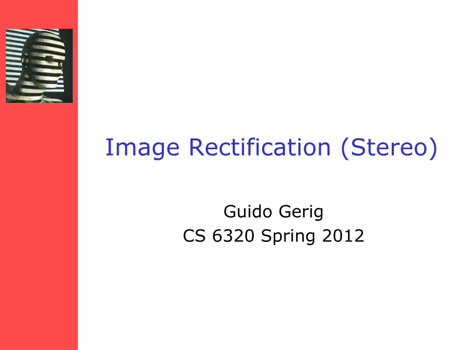
Image Rectification (Stereo)

Guido Gerig

CS 6320 Spring 2012

Example: converging cameras

courtesy of Andrew Zisserman

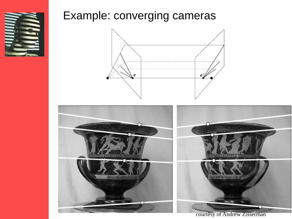
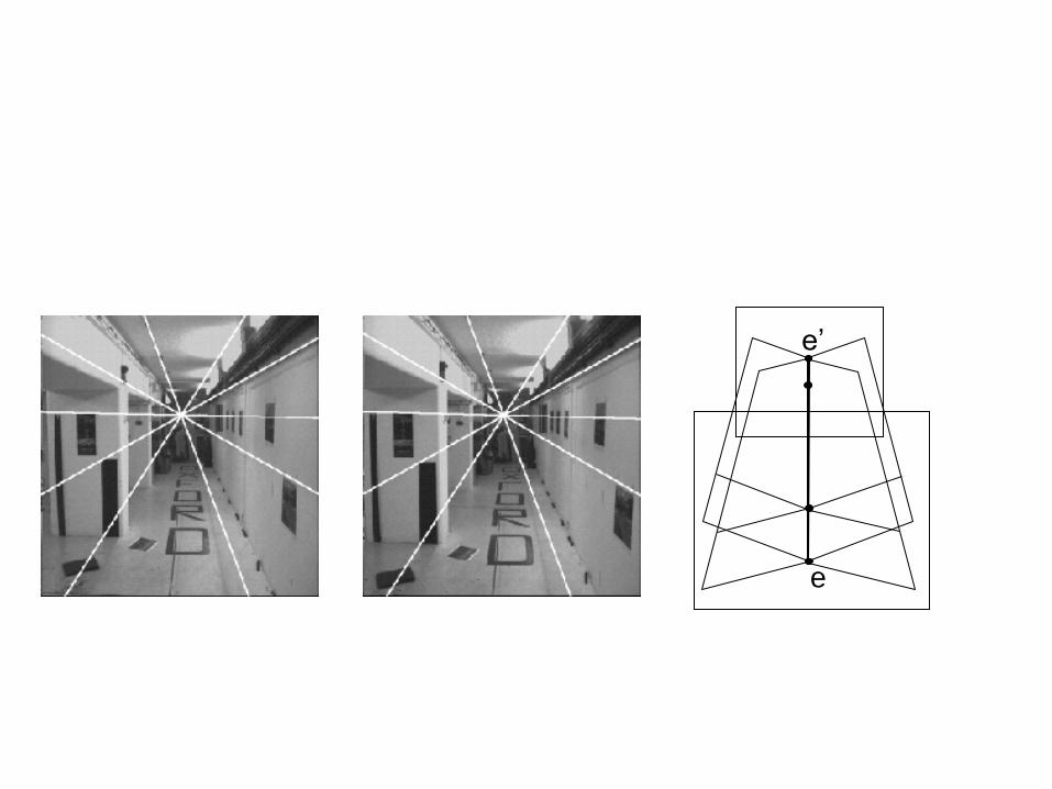
Epipolar Lines in Converging Cameras

Epipolar lines all intersect

at epipoles.

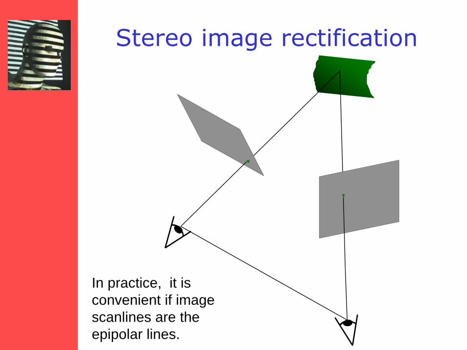
Stereo image rectification

In practice, it is

convenient if image

scanlines are the

epipolar lines.

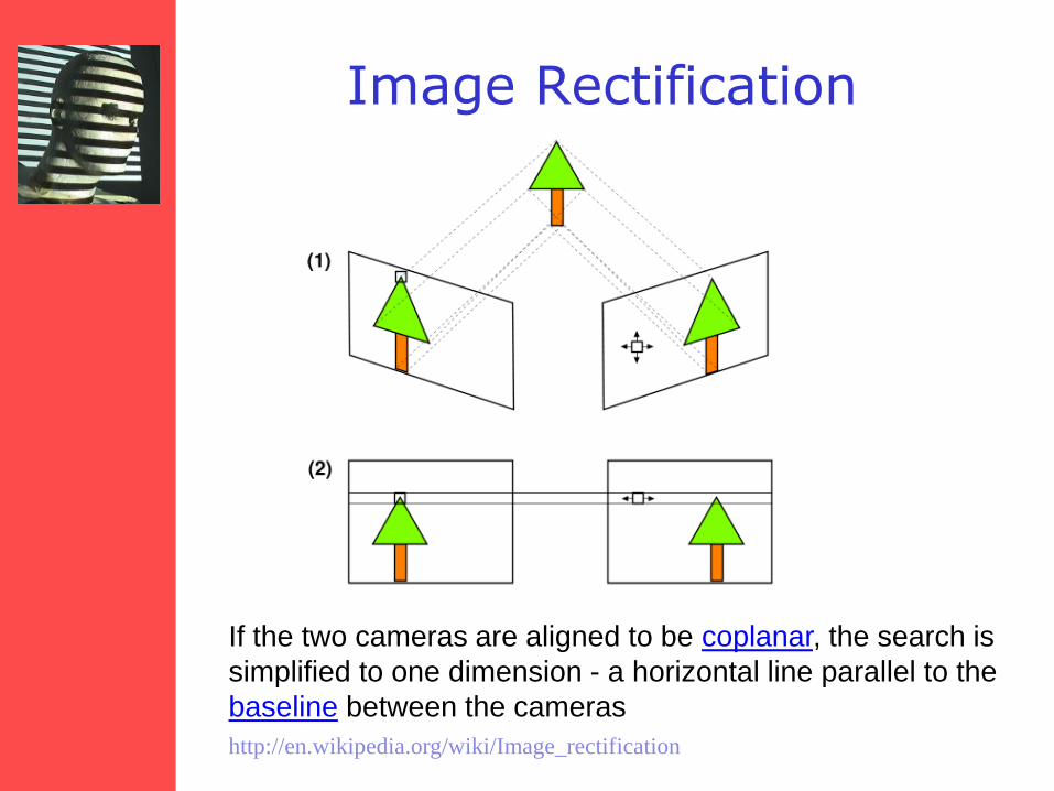
Image Rectification

http://en.wikipedia.org/wiki/Image_rectification

If the two cameras are aligned to be coplanar, the search is

simplified to one dimension - a horizontal line parallel to the

baseline between the cameras

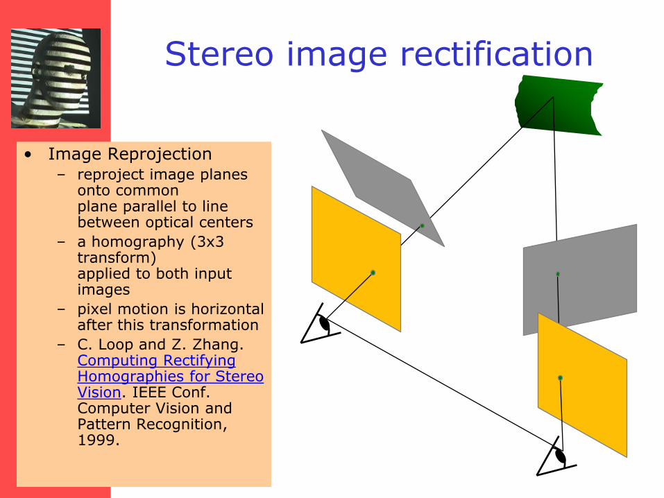
Stereo image rectification

• Image Reprojection – reproject image planes

onto common plane parallel to line between optical centers

– a homography (3x3 transform) applied to both input images

– pixel motion is horizontal after this transformation

– C. Loop and Z. Zhang. Computing Rectifying Homographies for Stereo Vision. IEEE Conf. Computer Vision and Pattern Recognition, 1999.

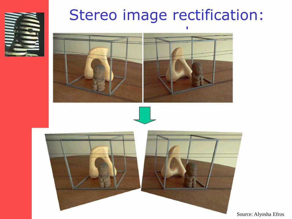
Stereo image rectification: example

Source: Alyosha Efros

ll

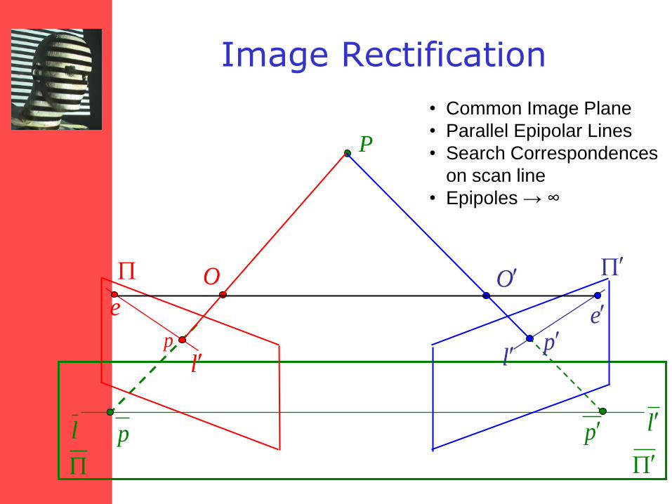
Image Rectification

pp

P

O O

l lp p

e e

• Common Image Plane

• Parallel Epipolar Lines

• Search Correspondences

on scan line

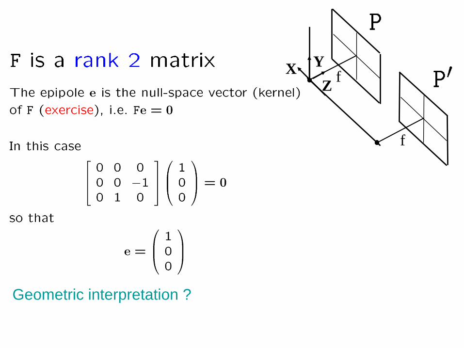
• Epipoles → ∞

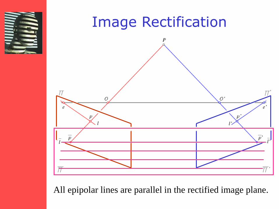
All epipolar lines are parallel in the rectified image plane.

Image Rectification

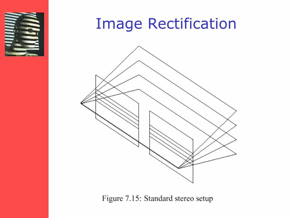
Image Rectification

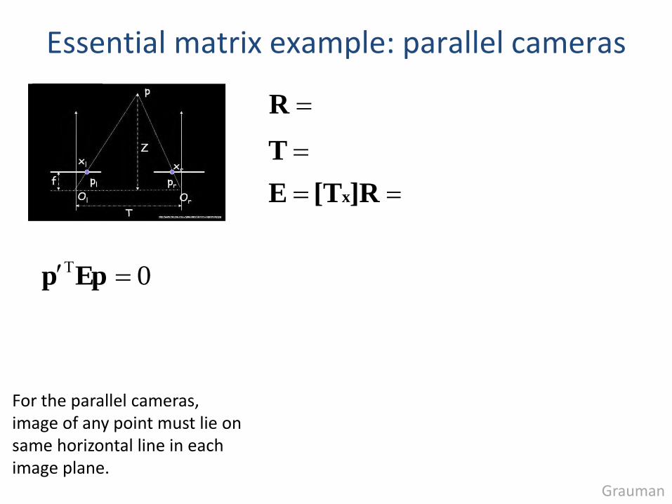
]R[TE

T

IR

x

]0,0,[ d0 0 0 0 0 d 0 –d 0

0Epp

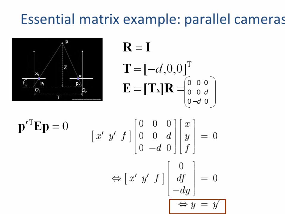
Essential matrix example: parallel cameras

For the parallel cameras, image of any point must lie on same horizontal line in each image plane.

Grauman

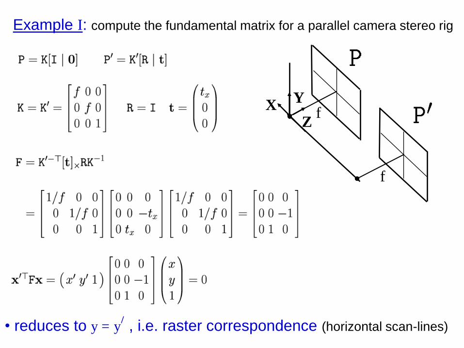
Example I: compute the fundamental matrix for a parallel camera stereo rig

• reduces to y = y/ , i.e. raster correspondence (horizontal scan-lines)

f

f

X Y

Z

f

f

X Y

Z

Geometric interpretation ?

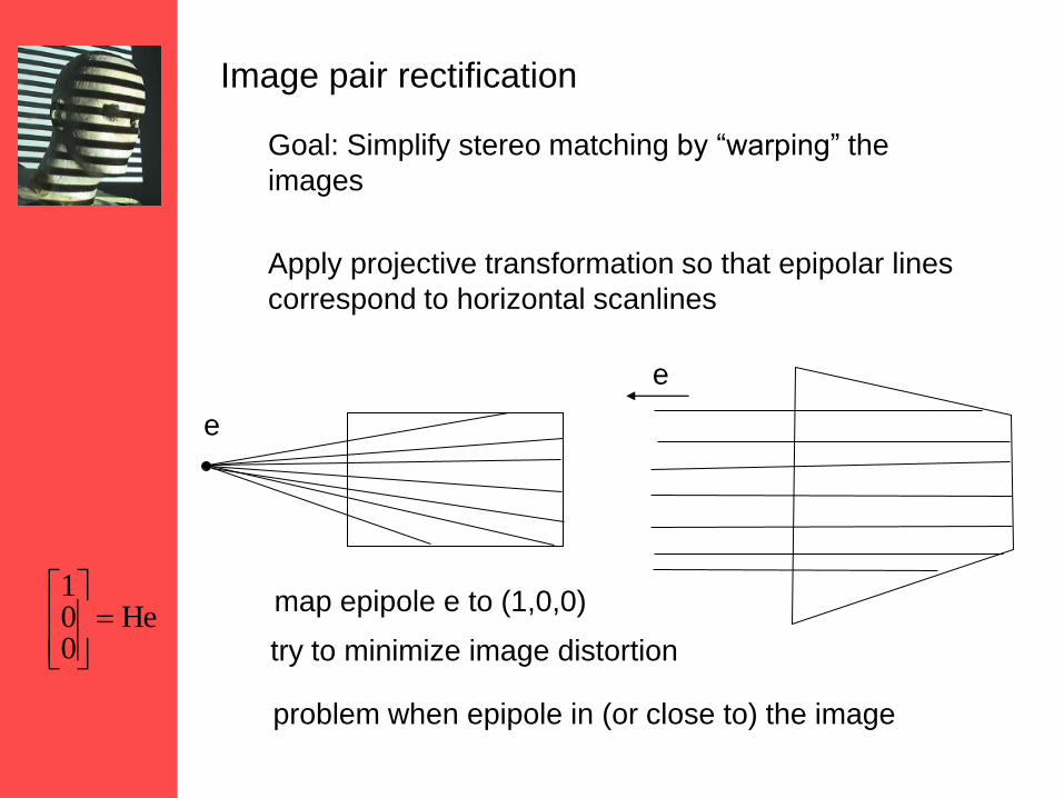
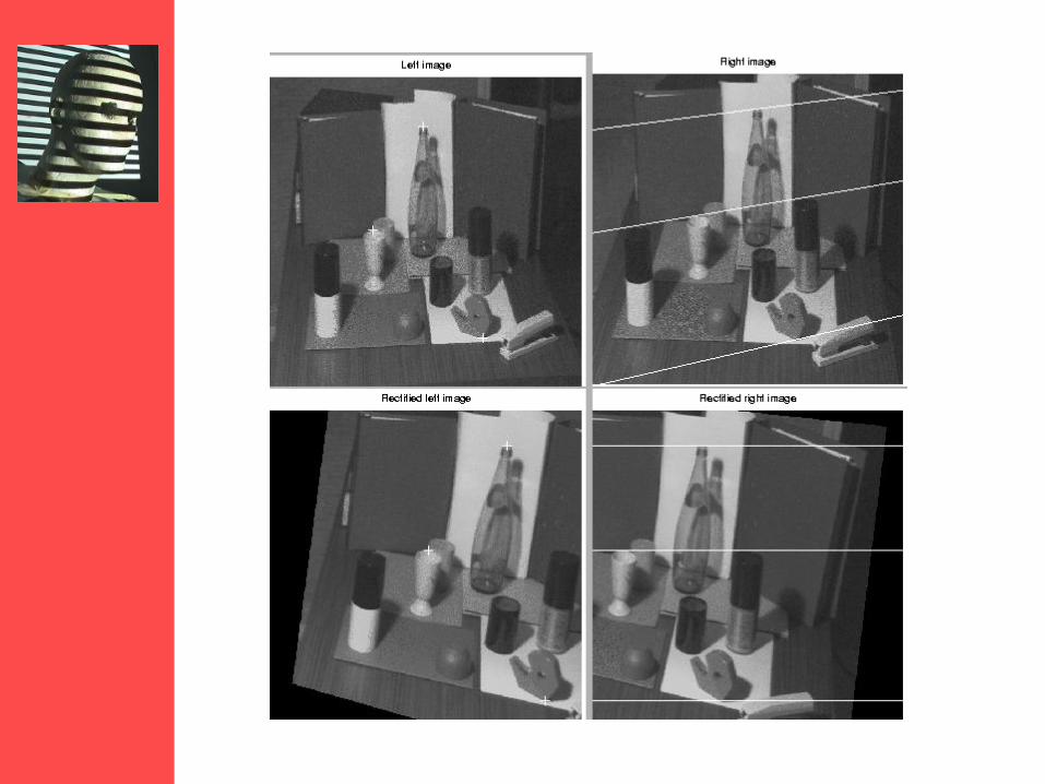
Image pair rectification

Goal: Simplify stereo matching by “warping” the

images

Apply projective transformation so that epipolar lines

correspond to horizontal scanlines

e

e

map epipole e to (1,0,0)

try to minimize image distortion

problem when epipole in (or close to) the image

He001

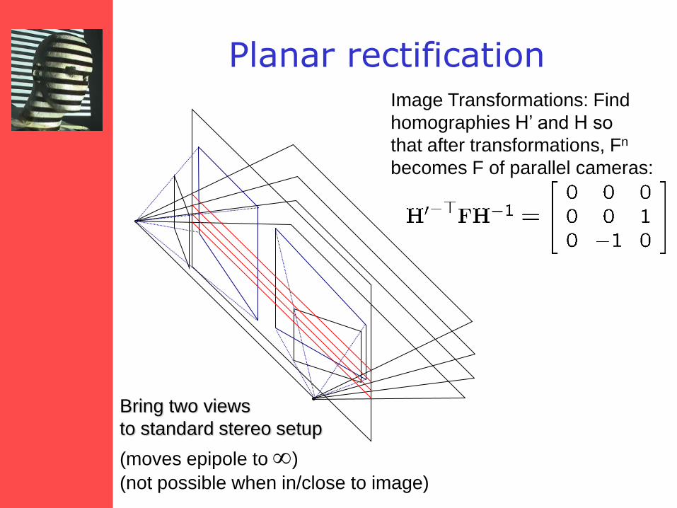
Planar rectification

Bring two views

to standard stereo setup

(moves epipole to )

(not possible when in/close to image)

Image Transformations: Find

homographies H’ and H so

that after transformations, Fn

becomes F of parallel cameras:

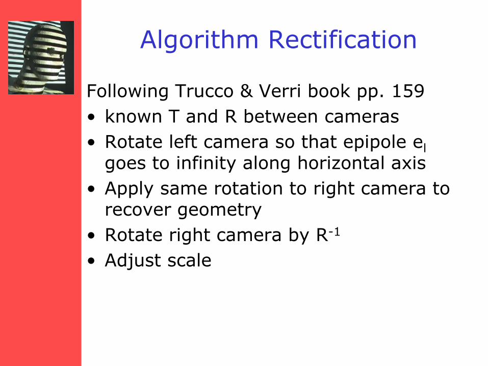
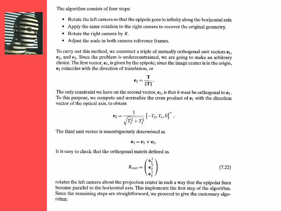
Algorithm Rectification

Following Trucco & Verri book pp. 159

• known T and R between cameras

• Rotate left camera so that epipole el goes to infinity along horizontal axis

• Apply same rotation to right camera to recover geometry

• Rotate right camera by R-1

• Adjust scale

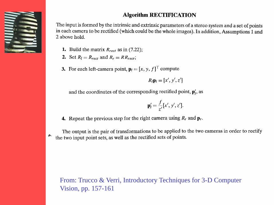
From: Trucco & Verri, Introductory Techniques for 3-D Computer

Vision, pp. 157-161

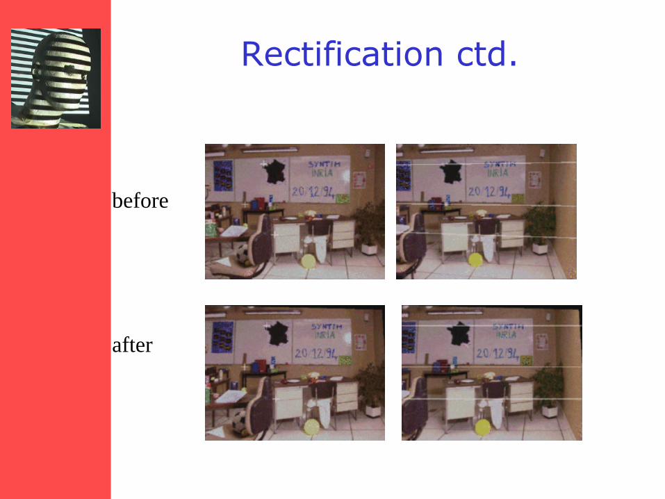
Rectification ctd.

before

after

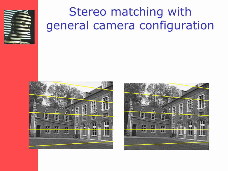
Stereo matching with general camera configuration

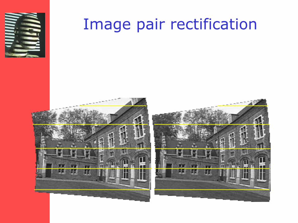
Image pair rectification

Other Material /Code

• Epipolar Geometry, Rectification: http://homepages.inf.ed.ac.uk/rbf/CVonline/LOCAL_COPIES/FUSIELLO2/rectif_cvol.html

• Fusiello, Trucco & Verri:Tutorial, Matlab code etc: http://profs.sci.univr.it/~fusiello/demo/rect/

25

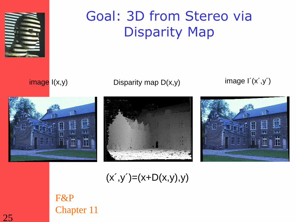
Goal: 3D from Stereo via Disparity Map

F&P

Chapter 11

image I(x,y) image I´(x´,y´) Disparity map D(x,y)

(x´,y´)=(x+D(x,y),y)

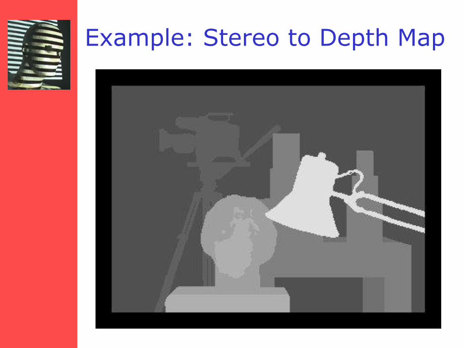
Example: Stereo to Depth Map

Run Example

Demo for stereo reconstruction (out of date): http://mitpress.mit.edu/e-

journals/Videre/001/articles/Zhang/CalibEnv/CalibEnv.html

Updated Webpages:

http://research.microsoft.com/en-

us/um/people/zhang/INRIA/softwares.html

SFM Example:

http://research.microsoft.com/en-

us/um/people/zhang/INRIA/SFM-Ex/SFM-Ex.html

Software:

http://research.microsoft.com/en-

us/um/people/zhang/INRIA/softwares.html

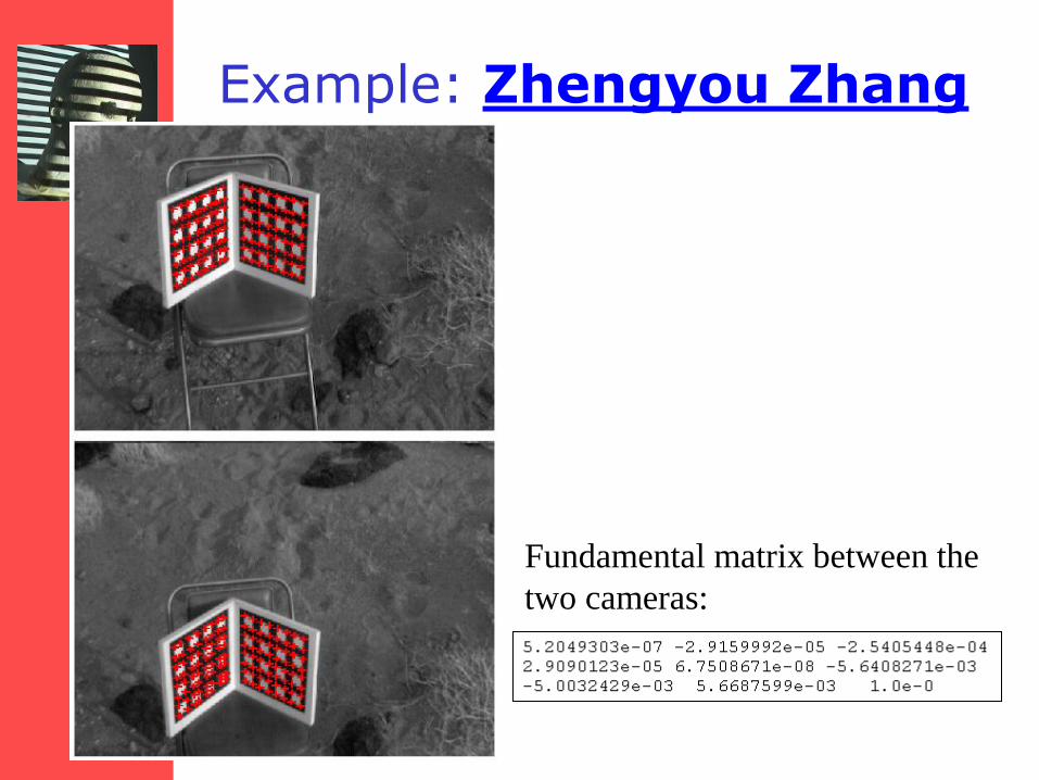
Example: Zhengyou Zhang

Fundamental matrix between the

two cameras:

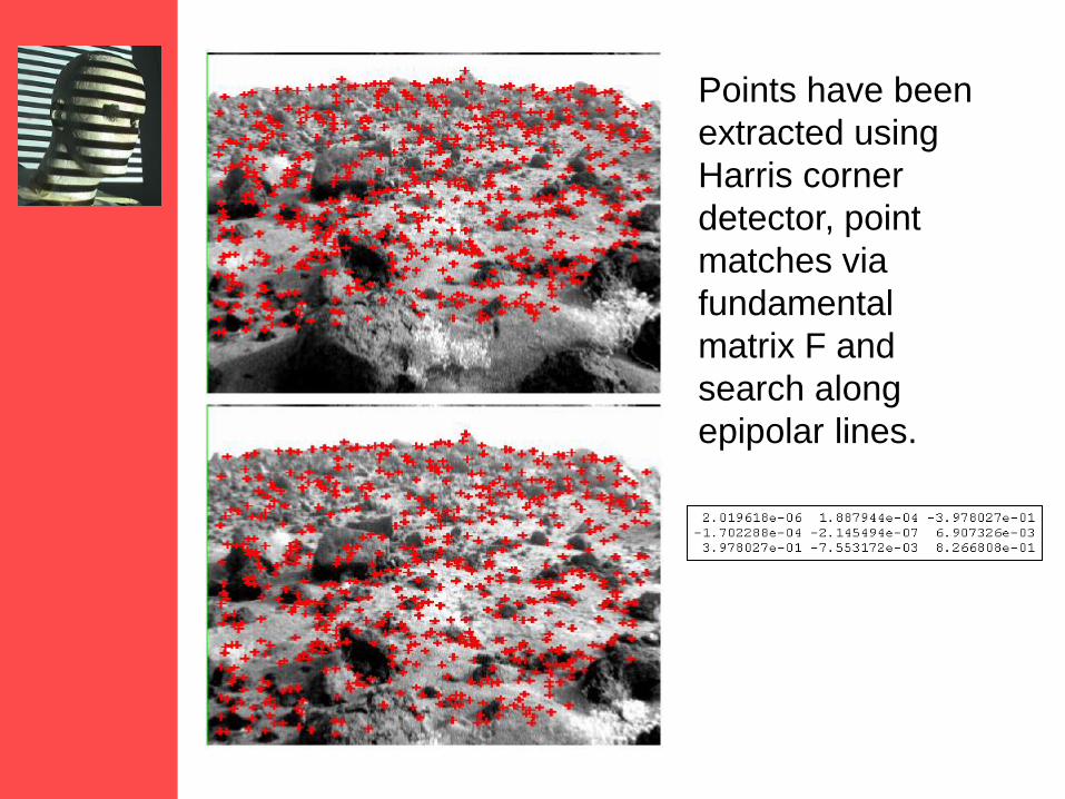
Points have been

extracted using

Harris corner

detector, point

matches via

fundamental

matrix F and

search along

epipolar lines.

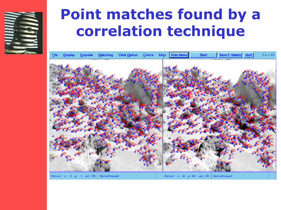
Point matches found by a correlation technique

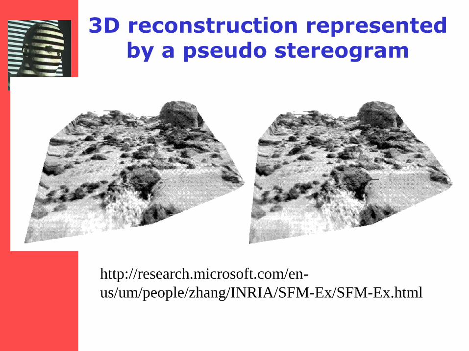
3D reconstruction represented by a pseudo stereogram

http://research.microsoft.com/en-

us/um/people/zhang/INRIA/SFM-Ex/SFM-Ex.html

Additional Materials: Forward

Translating Cameras

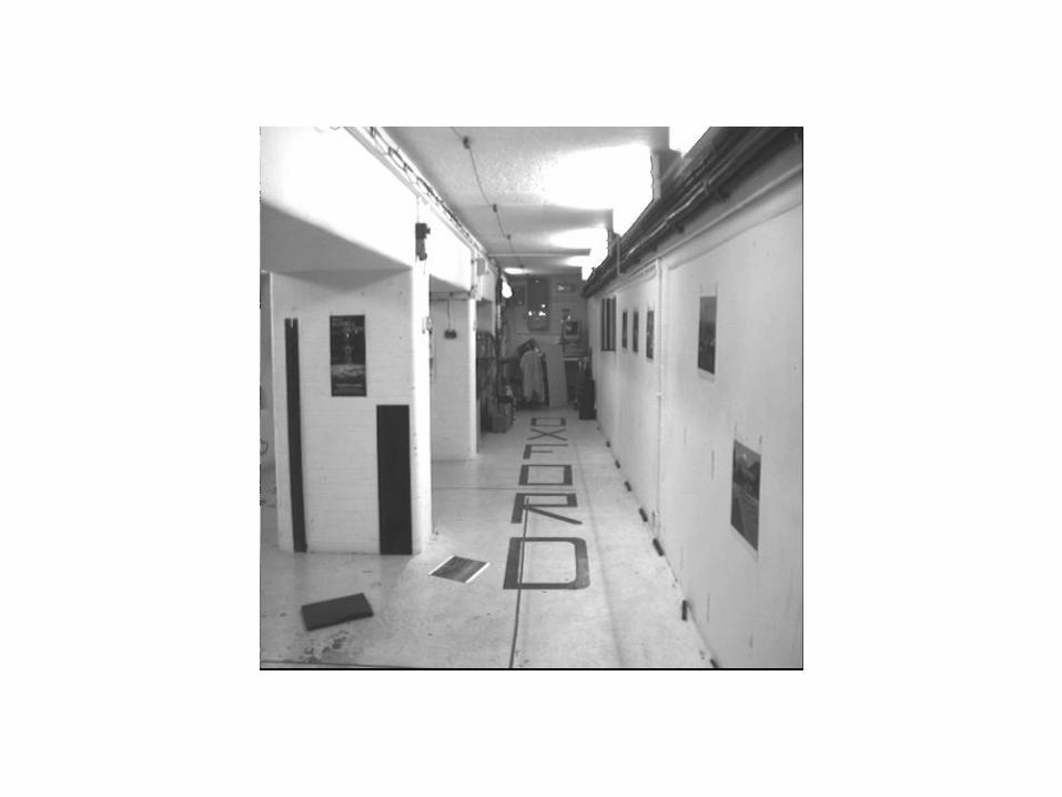
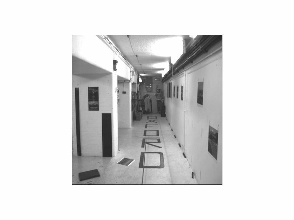
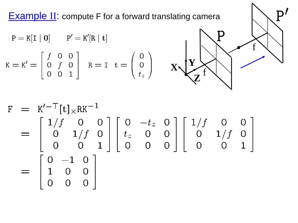
Example II: compute F for a forward translating camera

f

f

X Y

Z

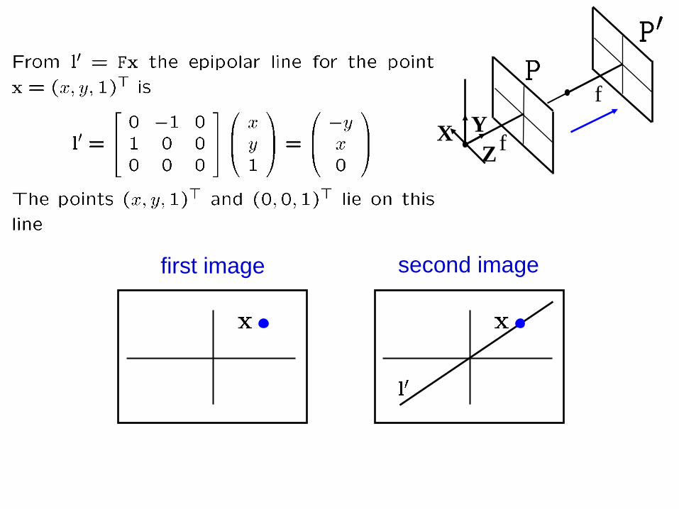
f

f

X Y

Z

first image second image

e

e’

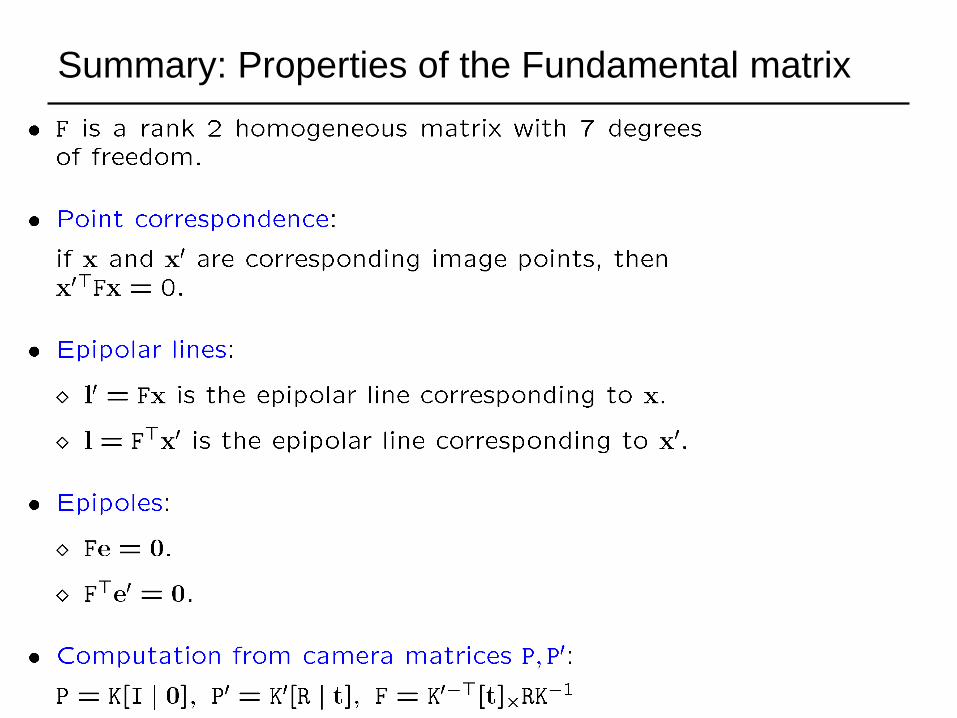
Summary: Properties of the Fundamental matrix