


Languages
Pages
Legal


Louisiana State UniversityLSU Digital Commons
LSU Doctoral Dissertations Graduate School
2008
Identification of quantitative trait loci influencingearly height growth in longleaf pine (Pinus palustrisMill)Lisha WuLouisiana State University and Agricultural and Mechanical College
Follow this and additional works at: https://digitalcommons.lsu.edu/gradschool_dissertations
Part of the Environmental Sciences Commons
This Dissertation is brought to you for free and open access by the Graduate School at LSU Digital Commons. It has been accepted for inclusion inLSU Doctoral Dissertations by an authorized graduate school editor of LSU Digital Commons. For more information, please [email protected].
Recommended CitationWu, Lisha, "Identification of quantitative trait loci influencing early height growth in longleaf pine (Pinus palustris Mill)" (2008). LSUDoctoral Dissertations. 3387.https://digitalcommons.lsu.edu/gradschool_dissertations/3387
i
IDENTIFICATION OF QUANTITATIVE TRAIT LOCI INFLUENCING EARLY HEIGHT GROWTH
IN LONGLEAF PINE (PINUS PALUSTRIS MILL)
A Dissertation
Submitted to the Graduate Faculty of the Louisiana State University and
Agricultural and Mechanical College in partial fulfillment of the
Requirements for the degree of Doctor of Philosophy
in
The School of Renewable Natural Resources
by Lisha Wu
B.S., China Agricultural University, China, 1998 M.S., China Agricultural University, China, 2001
M.S., Louisiana State University, USA, 2008 December 2008
nmqwertyuiopasdfghjklzxcvbnmqwertyuiopasdfghjklzxcvbnmqwertyuiopasdfghjklzxcvbnmqwertyuiopasdfghjklzx

ii
ACKNOWLEDGEMENTS
I take this wonderful opportunity to express my sincere gratitude and appreciation to Dr.
Michael Stine and Dr. Thomas Dean, co-chairs of my graduate committee, for their invaluable
guidance and for allowing me to obtain my Ph. D under their advisement. I will always be
grateful to Dr. Dana Nelson for taking time from his busy schedule to visit, help, and share his
invaluable ideas and knowledge to discuss with me from the initial experimental design to final
data analysis. I would like to thank and acknowledge Dr. Gerald Myers, Dr. Manjit Kang, and Dr.
Groth, Donald for their support, assistance, and guidance throughout the course of this study.
Special thanks and acknowledge to Mary Bowen, our research associate, for her
invaluable support and help in lab techniques, research method and data analysis. I gratefully
acknowledge the help of fellow graduate student Jatinder Atwal for his help in field data
collection. I also would like to thank Sedley Josserand for sharing her marker information with
me. Thanks are also due to Lynn Lott (retired), Larry Lott and Gay Flurry (Southern Institute of
Forest Genetics) for their technical assistance in crossing, seed and seedling processing, and field
testing. I thank Dr. James Geaghan, Dr. Brian Marx and Dr. David Blouin for their help on
statistical analyses. I would like to express my most sincere gratitude to Lucius W. Gilbert
Foundation for the financial support on this research.
Special thanks go to my husband Baogong Jiang for his love, support and encouragement.
I also want to take this chance to thank my mother, Caixia Lu, my father, Heng Wu and my
brother Xinyu Wu for their love and encouragement. Thanks everybody. This dissertation work
would have been exceedingly difficult without the motivation and assistance you provided.

iii
TABLE OF CONTENTS
ACKNOWLEDGEMENTS ............................................................................................................ ii
LIST OF TABLES ......................................................................................................................... vi
LIST OF FIGURES ..................................................................................................................... viii
LIST OF ABBREVIATIONS ......................................................................................................... x
ABSTRACT ................................................................................................................................... xi
CHAPTER 1 INTRODUCTION .................................................................................................... 1 1.1 Early Height Growth of Longleaf Pine ............................................................................ 1 1.2 The Genetic Improvement of EHG in Longleaf Pine ...................................................... 3 1.3 Marker-Assisted Selection ............................................................................................... 5 1.4 Molecular Marker ............................................................................................................ 6
1.4.1 Protein Markers ....................................................................................................... 7 1.4.2 DNA Markers .......................................................................................................... 8
1.4.2.1 Restriction Fragment Length Polymorphisms ................................................. 9 1.4.2.2 Random Amplified Polymorphic DNAs ....................................................... 10 1.4.2.3 Microsatellite or Simple Sequence Repeats .................................................. 12 1.4.2.4 Sequence Characterized Amplified Regions ................................................. 16 1.4.2.5 Amplified Fragment Length Polymorphisms ................................................ 16 1.4.2.6 Single Nucleotide Polymorphisms ................................................................ 16
1.5 Linkage Map and Mapping Theory ............................................................................... 18 1.5.1 Mapping Function ................................................................................................. 18 1.5.2 Mapping of Genetic Markers ................................................................................ 20 1.5.3 LOD Score ............................................................................................................ 21 1.5.4 Methods and Software Used in Genetic Mapping ................................................ 22 1.5.5 The Application of Linkage Maps in Genome Studies ......................................... 24
1.6 Quantitative Trait Loci and QTL Mapping .................................................................... 26 1.6.1 QTL Methods and Statistical Analysis ................................................................. 26
1.6.1.1 Single Marker Analysis ................................................................................. 26 1.6.1.2 Interval Marker Analysis ............................................................................... 27
1.6.2 QTL Pedigree and Strategies ................................................................................ 30 1.7 Future Perspective: From Linkage Map to QTLs .......................................................... 33 1.8 Research Objectives ....................................................................................................... 35 1.9 Outline of the Dissertation ............................................................................................. 36 1.10 References .................................................................................................................... 36
CHAPTER 2 SSR MARKER SCREEN AND POPULATION SELECTION ............................ 57 2.1 Introduction .................................................................................................................... 57 2.2 Materials and Methods ................................................................................................... 60
2.2.1 Plant Materials ...................................................................................................... 60 2.2.2 DNA Extraction, Purification and Quantification ................................................ 61 2.2.3 SSR Marker Sources and Preparation ................................................................... 63

iv
2.2.4 Preliminary Testing and Optimization of PCR Reaction Conditions ................... 64 2.2.5 Primer Screening ................................................................................................... 65 2.2.6 Planting Sites and Experimental Design ............................................................... 65 2.2.7 Field Data Collection ............................................................................................ 67 2.2.8 Statistical Analyses in Genetic Variance Estimation ............................................ 68
2.3 Results and Discussion................................................................................................... 69 2.3.1 Finding the Optimal Condition for PCR Amplification of SSRs ......................... 69 2.3.2 Molecular Marker Screen for Parents ................................................................... 73 2.3.3 Genetic Variance Estimation ................................................................................ 75 2.3.4 Population Selection ............................................................................................. 76 2.3.5 Selective Genotyping ............................................................................................ 78
2.5 References ...................................................................................................................... 78
CHAPTER 3 THE DEVELOPMENT OF AN INTEGRATED GENETIC MAP FOR LONGLEAF PINE COMPRISED OF MICROSATELLITE MARKERS .................................. 84
3.1 Introduction .................................................................................................................... 84 3.2 Materials and Methods ................................................................................................... 87
3.2.1 Plant Materials, DNA Isolation and Gel Electrophoresis ..................................... 87 3.2.2 Allele Frequencies and Parentage Test ................................................................. 87 3.2.3 Linkage Data Analyses ......................................................................................... 89 3.2.4 Locus Ordering and Map Construction................................................................. 89 3.2.5 Map Integration ..................................................................................................... 92 3.2.6 Estimation of Genome Length and Marker Coverage .......................................... 92
3.3 Results ............................................................................................................................ 94 3.3.1 Allele Frequencies and Parentage Analyses ......................................................... 94 3.3.2 Segregation of Markers ......................................................................................... 96 3.3.3 Construction of Linkage Map for the Individual Family .................................... 100 3.3.4 Integrated Maps from Six Full-Sib Families ...................................................... 106 3.3.5 Genome Length and Map Coverage ................................................................... 111
3.4 Discussion .................................................................................................................... 112 3.4.1 Heterozygosity and Polymorphic Information Content ...................................... 112 3.4.2 Segregation Distortion ........................................................................................ 113 3.4.3 The Integrated Map ............................................................................................. 115 3.4.4 Genome Length and Map Coverage ................................................................... 118
3.5 References .................................................................................................................... 119
CHAPTER 4 QTL MAPPING FOR GENES CONTROLLING EARLY HEIGHT GROWTH IN LONGLEAF PINE...................................................................................................................... 126
4.1 Introduction .................................................................................................................. 126 4.2 Materials and Methods ................................................................................................. 128
4.2.1 Plant Materials, DNA Isolation and Gel Electrophoresis ................................... 128 4.2.2 Statistical Analysis for Phenotypic Data............................................................. 129 4.2.3 QTL Identification .............................................................................................. 130
4.3 Results .......................................................................................................................... 131 4.3.1 Phenotypic Analysis of Height and Diameter ..................................................... 131 4.3.2 QTL Identification by Single Marker Analysis .................................................. 135 4.3.3 Phase I: QTL Detection by Interval Mapping ..................................................... 138

v
4.3.4 Phase II: QTL Verification by Interval Mapping ............................................... 140 4.4 Discussion .................................................................................................................... 143
4.4.1 Phenotypic Data .................................................................................................. 143 4.4.2 QTL Methods and Statistical Techniques ........................................................... 146 4.4.3 QTL Detection Population and Verification Population .................................... 148 4.4.4 QTLs Associated with Growth Traits ................................................................. 150
4.5 References .................................................................................................................... 153
CHAPTER 5 CONCLUSIONS AND FUTURE RECOMMENDATIONS .............................. 158 5.1 Conclusions .................................................................................................................. 158 5.2 Optimum Number of Markers and Minimum Number of Sample Size ...................... 159 5.3 QTL Mapping Approach .............................................................................................. 161 5.4 Application of Marker-assisted Selection in Tree Breeding ........................................ 163 5.5 References .................................................................................................................... 165
APPENDIX A: CTAB DNA ISOLATION PROTOCAL .......................................................... 168
APPENDIX B: ALLELE FREQUENCY FOR THE POLYMORPHIC MARKERS ............... 170
VITA ........................................................................................................................................... 174
vi
LIST OF TABLES
1.1 Mapping studies in forest trees with microsatellite markers ............................................. 15
1.2 Comparison of the most commonly used marker systems ................................................. 17
2.1 The F1 hybrid pedigree ...................................................................................................... 61
2.2 The pedigree and backcross code for crosses made in 2001 ............................................ 62
2.3 The pedigree and backcross code for crosses made in 2002 ............................................. 62
2.4 Possible marker genotype combinations and segregation pattern .................................... 66
2.5 The response variables used in data analyses .................................................................... 67
2.6 Summary of polymorphic markers that generate different loci information among parents .............................................................................................. 74
2.7 Number of informative polymorphic SSR markers within each family ............................ 74
2.8 Genetic variance estimation results for height variables from two different methods ............................................................................................................... 77
3.1 Genotype codes for a CP population ................................................................................. 90
3.2 Summary for allele frequency estimation obtained from CERVUS .................................. 94
3.3 Number of informative polymorphic SSR markers within each family ............................ 97
3.4 Chi-square test for distorted markers and their distribution in linkage groups .................. 98
3.5 Comparison of linkage groups, marker numbers, genetic length and mean interval between markers in the SSR-based linkage map for each full-sib family ....................... 102
3.6 Comparison of marker numbers, genetic length, and mean interval between markers in the SSR-based linkage map for integrated map (Haldane’s mapping function) .......... 107
3.7 Comparison of marker numbers, genetic length, and mean interval between markers in the SSR-based linkage map for integrated map (Kosambi’s mapping function) ............. 108
4.1 ANOVA table for different environments for height (ht4) .............................................. 132
4.2 Mean estimation of the height (cm) for individual full-sib familiy at different environments after being planted for four years .............................................................. 132
vii
4.3 Correlation coefficient for total heights and diameters in the Derr488 half-sib family .................................................................................................................. 135
4.4 Linkage group, marker loci, and single-locus point effects of SSR markers significantly associated with the QTLs using simple regression approach ..................... 136
4.5 Intervals detected that contain QTLs influencing growth traits by QTL Express for QTL detection population ............................................................................. 138
4.6 Intervals detected that contain QTLs influencing growth traits by QTL Express for QTL verification population ........................................................................ 142
A.1 Solutions for DNA extraction .......................................................................................... 169
B.1 The allele frequency test for polymorphic markers form software CERVUS ................. 170
viii
LIST OF FIGURES
1.1 Brown spot needle blight (Scirrhia acicola) in longleaf grass-stage. .................................. 2
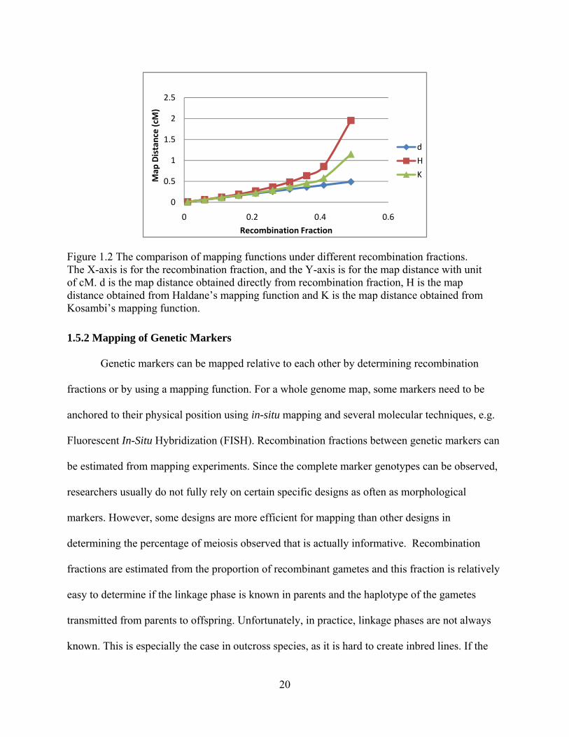
1.2 The comparison of mapping functions under different recombination fractions. ............. 20
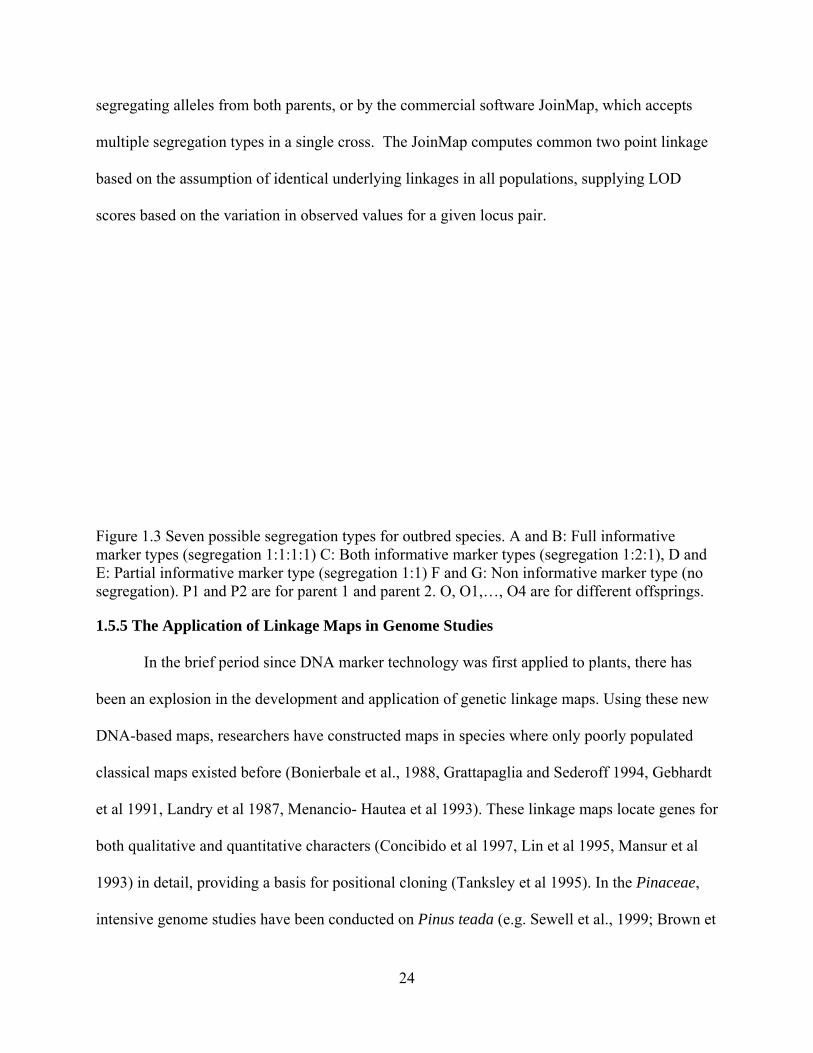
1.3 Seven possible segregation types for outbred species. ...................................................... 24
2.1 The effect of PIG tailing to the primer RPtest09 on PCR amplification. .......................... 70
2.2 The effects of Taq polymerases on PCR amplification ..................................................... 70
2.3 The effect of Mg2+ on PCR amplification .......................................................................... 72
2.4 The effect of initial annealing temperature on PCR amplification .................................... 72
2.5 The probability plot for parent, location, and parent x location effects. ............................ 76
3.1 The scatter plot of the PIC value (A) and the expected heterozygosity (B) with the change of number of alleles per locus................................................................. 96
3.2 Comparison of linkage group for individual full-sib mapping populations. ................... 103
3.3 An integrated SSR-based genetic map constructed by 110 polymorphic SSR markers with Haldane’s mapping function. .............................................................. 109
3.4 An integrated SSR-based genetic map constructed by 110 polymorphic SSR markers with Kosambi’s mapping function. ............................................................. 110
3.5 The distribution of interval distance between adjacent markers for the integrated map. .................................................................................................................. 112
3.6 Multiple locus SSR markers ............................................................................................ 115
4.1 Frequency distributions of height growth (left) and the corresponding residual height growth (right). ......................................................................................... 133
4.2 Frequency distributions of diameter (left) and the corresponding residual diameter (right). ................................................................................................................ 134
4.3 The plot for explained variance for 5 growth traits for a QTL detection population.. ...................................................................................................................... 139
4.4 The overplot of QTLs for growth traits detected by interval mapping with QTL Express for QTL detection population. ........................................................... 141
ix
4.5 The plot for explained variance for 5 growth traits for QTL detection population. ........ 143
4.6 The overplot of QTLs for growth traits detected by interval mapping with QTL Express for QTL verification population ........................................................ 144
4.7 The QTLs were detected and verified by 3 populations and 2 methods at different linkage groups.. ............................................................................................. 145
4.8 The Hurricane Katrina Damaged Tree Recovery in Jan, 2006. ....................................... 152
5.1 Optimal distance between target locus and flanking markers. ........................................ 160
x
LIST OF ABBREVIATIONS
AFLP Amplified Fragment Length Polymorphisms
ANOVA Analysis of Variance
CCGP Conifer Comparative Genomic Project
CIM Composite Interval Mapping
DH Double Haploid
EHG Early Height Growth
EST Expressed Sequence Tag
GAS Gene-Assisted Selection
IBD Identity–by–Descent
IM Interval Mapping
LD Linkage Disequilibrium
LOD Log of Odds
LS Least Square
MAS Marker-Assisted Selection
ML Maximum Likelihood
MQM Multiple QTLs Model
OP Open Pollinated
PCR Polymerase Chain Reaction
PIC Polymorphism Information Content
QTL Quantitative Trait Loci
QTN Quantitative Trait Nucleoid
RAPD Random Amplified Polymorphic DNA
RFLP Restriction Fragment Length Polymorphisms
RIL Recombinant Inbred Lines
SA Simulated Annealing
SCAR Sequence Characterized Amplified Regions
SNP Single Nucleotide Polymorphisms
SSR Simple Sequence Repeat
TGOP Three Generation Outbreed Pedigree
xi
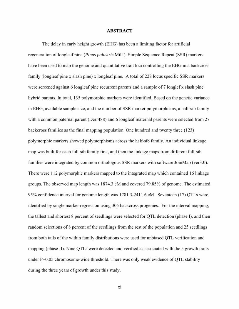
ABSTRACT
The delay in early height growth (EHG) has been a limiting factor for artificial
regeneration of longleaf pine (Pinus palustris Mill.). Simple Sequence Repeat (SSR) markers
have been used to map the genome and quantitative trait loci controlling the EHG in a backcross
family (longleaf pine x slash pine) x longleaf pine. A total of 228 locus specific SSR markers
were screened against 6 longleaf pine recurrent parents and a sample of 7 longlef x slash pine
hybrid parents. In total, 135 polymorphic markers were identified. Based on the genetic variance
in EHG, available sample size, and the number of SSR marker polymorphisms, a half-sib family
with a common paternal parent (Derr488) and 6 longleaf maternal parents were selected from 27
backcross families as the final mapping population. One hundred and twenty three (123)
polymorphic markers showed polymorphisms across the half-sib family. An individual linkage
map was built for each full-sib family first, and then the linkage maps from different full-sib
families were integrated by common orthologous SSR markers with software JoinMap (ver3.0).
There were 112 polymorphic markers mapped to the integrated map which contained 16 linkage
groups. The observed map length was 1874.3 cM and covered 79.85% of genome. The estimated
95% confidence interval for genome length was 1781.3-2411.6 cM. Seventeen (17) QTLs were
identified by single marker regression using 305 backcross progenies. For the interval mapping,
the tallest and shortest 8 percent of seedlings were selected for QTL detection (phase I), and then
random selections of 8 percent of the seedlings from the rest of the population and 25 seedlings
from both tails of the within family distributions were used for unbiased QTL verification and
mapping (phase II). Nine QTLs were detected and verified as associated with the 5 growth traits
under P=0.05 chromosome-wide threshold. There was only weak evidence of QTL stability
during the three years of growth under this study.
1
CHAPTER 1 INTRODUCTION
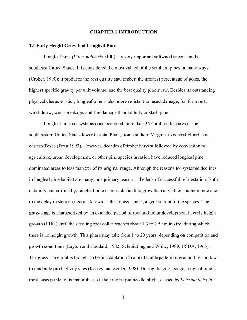
1.1 Early Height Growth of Longleaf Pine
Longleaf pine (Pinus palustris Mill.) is a very important softwood species in the
southeast United States. It is considered the most valued of the southern pines in many ways
(Croker, 1990): it produces the best quality saw timber, the greatest percentage of poles, the
highest specific gravity per unit volume, and the best quality pine straw. Besides its outstanding
physical characteristics, longleaf pine is also more resistant to insect damage, fusiform rust,
wind-throw, wind-breakage, and fire damage than loblolly or slash pine.
Longleaf pine ecosystems once occupied more than 36.4 million hectares of the
southeastern United States lower Coastal Plain, from southern Virginia to central Florida and
eastern Texas (Frost 1993). However, decades of timber harvest followed by conversion to
agriculture, urban development, or other pine species invasion have reduced longleaf pine
dominated areas to less than 5% of its original range. Although the reasons for systemic declines
in longleaf pine habitat are many, one primary reason is the lack of successful reforestation. Both
naturally and artificially, longleaf pine is more difficult to grow than any other southern pine due
to the delay in stem elongation known as the “grass-stage”, a genetic trait of the species. The
grass-stage is characterized by an extended period of root and foliar development in early height
growth (EHG) until the seedling root collar reaches about 1.3 to 2.5 cm in size, during which
there is no height growth. This phase may take from 1 to 20 years, depending on competition and
growth conditions (Layton and Goddard, 1982; Schmidtling and White, 1989; USDA, 1965).
The grass-stage trait is thought to be an adaptation to a predictable pattern of ground fires on low
to moderate productivity sites (Keeley and Zedler 1998). During the grass-stage, longleaf pine is
most susceptible to its major disease, the brown-spot needle blight, caused by Scirrhia acicola
2
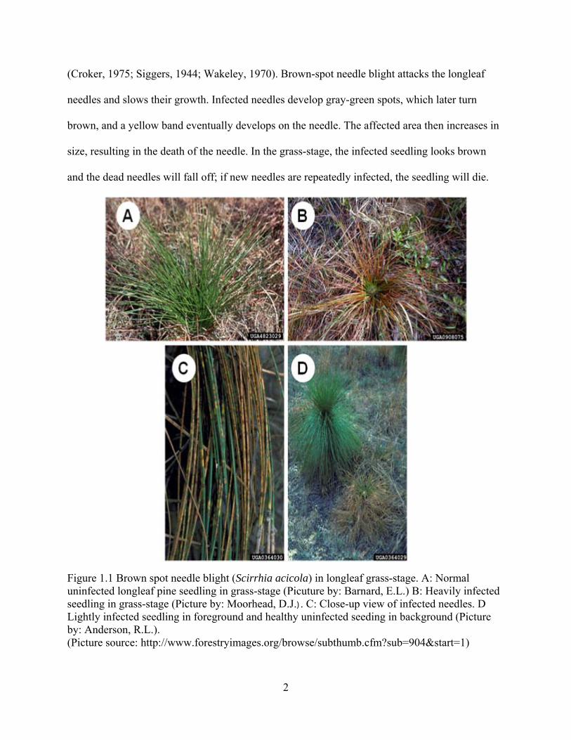
(Croker, 1975; Siggers, 1944; Wakeley, 1970). Brown-spot needle blight attacks the longleaf
needles and slows their growth. Infected needles develop gray-green spots, which later turn
brown, and a yellow band eventually develops on the needle. The affected area then increases in
size, resulting in the death of the needle. In the grass-stage, the infected seedling looks brown
and the dead needles will fall off; if new needles are repeatedly infected, the seedling will die.
Figure 1.1 Brown spot needle blight (Scirrhia acicola) in longleaf grass-stage. A: Normal uninfected longleaf pine seedling in grass-stage (Picuture by: Barnard, E.L.) B: Heavily infected seedling in grass-stage (Picture by: Moorhead, D.J.). C: Close-up view of infected needles. D Lightly infected seedling in foreground and healthy uninfected seeding in background (Picture by: Anderson, R.L.). (Picture source: http://www.forestryimages.org/browse/subthumb.cfm?sub=904&start=1)

3
The delay in EHG for the grass-stage has drawn the attention of scientists for a long time.
Experiments in improving nursery technique, seedling care, and silvicultural practices have all
been shown to have positive effects (Shipman, 1960; Smith and Schmidtling, 1970).
Nevertheless, none of these improvements has been widely used in practice due to investment
cost, labor and environmental limitations.
1.2 The Genetic Improvement of EHG in Longleaf Pine
Breeding programs have been underway for more than 35 years to improve brown-spot
resistance and early height growth of longleaf pine (Bey and Snyder, 1978). Longleaf pine is a
highly variable species, and a considerable proportion of this variation is genetic. Considering
the economically important traits, longleaf pines have as much or more genetic variation than
other southern pines (Snyder and Derr, 1977). However, the development of such resources is
hampered by the long generation interval, outcrossing mating system, and high genetic load,
typical of forest tree species. Furthermore, traditional forest tree improvement methods have
exclusively relied on phenotypic selection, expensive long-term field progeny testing for
phenotypic traits, and generally elaborate statistical analysis of the data. Summaries of progress
using basic tree breeding methods (Jett 1988, Zobel and Talbert, 1984) have shown them to be
effective yet slow (Tauer and Hallgren, 1992; Krugman, 1985).
Since this grass-stage condition is a unique characteristic of longleaf pine (Schmidtling
and White, 1989); it may be improved by interspecific hybridization. Both slash pine (Pinus
elliottii Engl.) and loblolly pine (Pinus taeda L.) are potential donors of EHG genes because of
their early maturity and fast growing characteristics. Natural hybridization is common between
longleaf pine and loblolly pine, producing the Sonderegger pine (Pinus × sondereggeri H.H.
Chapm), which is the only named southern pine hybrid. Natural hybridization between longleaf
4
pine and slash pine is unlikely, based on differences between the species in dormancy and heat
requirement for stroboli develeopment (Boyer, 1981). However, artificial crosses between
longleaf pine and slash pines can be achieved easily (Boyer, 1990) and the variation in EHG was
found to be significant among and within families in several field tests of longleaf pine x slash
pine hybrids (Derr 1966; Derr, 1969). Slash pine is one of the fastest growing and earlier-
maturing species, but it is also very sensitive to fusiform rust. Lohrey (1990) referred to the
longleaf x slash hybrid as showing the most potential because height growth began quickly,
almost as fast as slash pine, and it was fairly resistant to both brown-spot needle disease and
fusiform rust. Derr (1966) has indicated that the hybridization between longleaf pine and slash
pine to improve EHG was practicable; the survival, growth, and disease susceptibility of longleaf
pine x slash pine hybrids are improved. For example, the average height for wind–pollinated
slash pine and wind-pollinated longleaf at age 4 was 2.4 and 0.8 m, respectively, while the
longleaf pine and slash pine hybrid was 2.3 m. Most traits for these hybrids were intermediates
between longleaf pine and slash pine. Several generations of backcrosses were needed in order to
replace the slash pine portion of the hybrid genome, other than those genes regulating the early
height growth. The hybrids that show desired phenotype were selected for recurrent backcrosses.
For one generation of backcrossing, fifty percent of the longleaf pine genome was recovered, and
5 or 6 generations of backcrosses gave a reasonable genome recovery.
However, forest tree breeding traditionally has been viewed as an application of
quantitative genetics (Zobel and Talbert 1984). Previous studies have shown that EHG in
longleaf pine is a quantitative trait, controlled by a small number of major effect genes (Brown
1964; Weng, et al., 1999; Nelson, 2003) with heritability (h2 ) ranging from 0.47 to 0.68
(Layton and Goddard 1982; Snyder and Namkoong 1978). Gain from phenotypic selection is
5
limited when h2 is small because the limited proportion of genetic variance the breeder can
capture at an early stage. Taking into account the long generation interval and linkage drag
associated with the selection, to select all the major QTLs using traditional methods would be
time-consuming and destructive.
1.3 Marker-Assisted Selection
The use of molecular marker-assisted selection (MAS) are currently utilized in crop and
animal breeding, and they also promise to be useful in studies on forest trees that are directed
towards obtaining faster genetic improvement in timber quality (Brown, 2003), growth rate
(Emebiri, 1997), and stress and disease tolerance (Grattapaglia and Sedero, 1994; Plomion, et al.,
1996). The MAS is based on the establishment of a linkage relationship between the easily
scorable molecular markers and the characteristics of interest. If markers that are linked to the
major QTL can be identified, then these markers can be used to guide the selection of the hybrid
and the subsequent backcross generations. The use of DNA markers for indirect selection offers
the greatest benefits for quantitative traits with low heritability, as these are the most difficult
characters to assess in field experiments. The three essential requirements for MAS in a breeding
program are: first, markers should co-segregate or be closely linked with the target gene (within
2 cM or less); and second, an efficient means of screening large populations for the molecular
markers should be available; and thirdly the screening technique should have high
reproducibility across laboratories, be economical to use and be user-friendly (Mohan, et al.,
1997).
Compared with the tradition breeding program, MAS has many advantages. It provides a
way to increase the efficiency of within family selection by exploring simultaneous selection for
multiple traits by selecting makers that are tightly linked to the QTLs of interest. It allows

6
selection at the juvenile stage from an early generation and the unfavorable alleles can be
eliminated or greatly reduced during the early stages of development. The most straightforward
application of molecular markers in MAS includes genetic distance analysis, variety
identification, identification of markers tightly linked to specific genes, and MAS backcrossing. I
will focus on the last two functions in this project.
The future of MAS aims not only at utilizing perfect markers for improving existing
breeding schemes, e.g., backcrossing, but also controlling all allelic variation for all genes of
agronomic relevance. In a simulation study of building superior genotypes, Peleman and van der
Voort (2003) introduced a concept, “breeding by design”, that requires the knowledge of the map
position of all loci of agronomic importance, the allelic variation at those loci, and their
contribution to the genotype. Although great efforts have to be made to gather all this
information of precise genetic stocks, such as introgression line libraries (Eshed and Zamir 1995)
for mapping, all relevant traits are available for several crop plants. Additionally, allelic variation
at any locus in the genome can be assessed by establishing haplotypes of multiple tightly linked
markers. This all embracing approach has to be addressed immediately to make molecular
markers an accepted and irreplaceable tool for developing better crop plants.
1.4 Molecular Marker
Since Mendel formulated his law of inheritance in 1865, it has been a core component of
biology to relate genetic factors to functions visible as phenotypes. People have been monitoring,
inducing, and mapping single gene markers in plants, animals, and human beings. In early
research, most of the single gene markers used in plant genetics were those either affecting
morphological characters (i.e. morphological markers) or changing the structure and number of
chromosomes (i.e. cytological markers). These types of markers generally correspond to
7
qualitative traits that can be scored visually, such as seed color, leaf shape, or chromosome
deletion, duplication, inversion, and translocation. These traits occur naturally, but can also be
generated from mutagenesis experiments. These kinds of markers have been found useful in the
linkage map construction of forest trees (Chaparro et. al., 1994; Jermstad et al., 1994). Though
the markers have served well in various types of basic and applied research, their use in many
areas of plant breeding has been very limited (reviewed by Tanksley, 1983). These markers are
usually affected by the environment and developmental stage, limited in number. Moreover, the
genes controlling these markers can have pleiotropic effect on the character under investigation
which eludes the actual location of genes due to distortion of segregation rations.
The development in recent years of molecular markers offers the possibility of finding
new approaches to breeding procedures. The molecular markers are heritable molecules that
mark loci on chromosomes and reveal polymorphisms at the protein or DNA level. To be a
useful molecular marker, it must be polymorphic, reproducible, preferably display co-dominant
inheritance (both forms detectable in heterozygote), and fast and inexpensive to detect. The
marker methods differ with respect to the type, specificity, volume of genetic data generated, lab
time required, and the cost of equipment and materials. Based on the level at which the genes are
detected, molecular markers can be divided into two classes: protein markers and DNA markers.
1.4.1 Protein Markers
Protein markers code for proteins that can be separated by electrophoresis to determine
the presence or absence of specific alleles. The most widely used protein markers in plants are
allozyme. Isozyme are an allelic variant of enzymes encoded by structural genes and provide a
relatively simple and inexpensive method of obtaining genetic information. The first linkage
studies of Pinus were based on the segregation of isozyme extracted from megagametophytes.

8
More than 10 species have been studied for about 15 loci (Guries et al., 1978; Rudin and
Eckberg, 1978; O’Malley et al., 1979; Ekert et al., 1981; Cheliak, et al., 1984; O’Malley et al.,
1986; Furmier et al., 1986; Strauss and Conkle, 1986; El-Kassaby et al., 1987; Shiraishi, 1988;
Szmidt et al., 1989; Hamrick et al., 1992). A 2D-PAGE of the total proteins of
megagametophytes allowed studying of a much large number of loci than had been previously
possible with isozyme analysis (Anderson et al., 1985; Bahrman and Damerval, 1989; Gerber et
al., 1993). However, their application is limited by the number of enzyme loci, the low levels of
variability in some species, poorly understood modes of inheritance and developmental
instability (Bahrman and Damerval, 1989), and the fact that they only reveal variation in enzyme
genes (Tanksley, et al., 1989). These limitations lead several groups to use other types of
molecular markers.
1.4.2 DNA Markers
Scientists are constructing genetic linkage maps composed of DNA markers for a wide
range of plant species (O’Brien, 1993). Several types of DNA markers have been widely used:
restriction fragment length polymorphisms (RFLPs) (Bostein et al., 1980), random amplified
polymorphic DNAs (RAPDs) (Williams et al., 1990), simple sequence repeat (SSRs or
microsatellite) (Litt and Luty 1989), amplified fragment length polymorphisms (AFLPs) (Vos et
al 1995), and single nucleotide polymorphisms (SNPs) (Wang et al 1998). All types of DNA
markers detect sequence polymorphisms and monitor the segregation of a DNA sequence among
progenies of a genetic cross in order to construct a linkage relationship. The most commonly
used DNA markers are RFLPs and RAPDs. In the last ten years, however, usage of such markers
as AFLPs, SSRs, and SNPs has also become widespread.

9
Each DNA marker method analyzes different aspects of DNA sequence variations and
different regions of the genomes. For example, RFLPs were detected using cDNA clones,
namely the coding sequence, but were also frequently detected in variations that lay in regions
flanking the genes. SSR markers have generally been from non-coding regions, although the
recent move to three base repeats and the use of expressed sequence tags (ESTs) as the source of
SSR markers is changing this standard. Other markers, such as RAPD and AFLP markers,
frequently appear in repetitive regions of the genome. In some cases, the stability of the sequence
difference may also be an issue. SSRs are seen as being unstable for some applications since the
mutation rate may be high in certain criteria. The decision about the most appropriate marker
system to use varies greatly depending on the species, the objective of the marker work, and the
resources available.
1.4.2.1 Restriction Fragment Length Polymorphisms
RFLPs are fragments of restricted DNA (usually within the 2~10 kb range) separated by
gel electrophoresis and detected by subsequent Southern blot hybridization to a radio-labeled
DNA probe. The probe consists of a sequence of unknown identity or part of the sequence of a
cloned gene, which is obtained by molecular cloning and isolation of suitable DNA fragments.
Polymorphisms are visualized as differences in banding patterns between or among two or more
individuals. RFLPs were first used in human genome mapping (Botstein et al., 1980), and it was
later adopted for plant genome study.
RFLPs are the most reliable polymorphisms which can be used for accurate scoring of
genotypes. They are co-dominant and highly reproducible, which make them useful in
identifying a unique locus. RFLP methods are well suited for species maps because the same
hybridization probes can be used for comparison among species (Ahuja et al., 1994; Byrne et al.,

10
1995; Jermstad et al., 1994). Because of their high genomic abundance and random distribution
throughout the genome, RFLPs have frequently been used in gene mapping studies of various
plant species, although few studies were reported in trees. Devey et al. (1994) presented linkage
groups in loblolly pine for 80 RFLPs detected using cDNA probes. Linkage maps using mostly
RFLP markers have been recently presented for poplar (Bradshaw et al., 1994; Jorge et al., 2005),
Douglas-fir (Jermstad et al., 1994), pine (Nance and Nelson, 1989; Neale, 1991, 1994; Devey et
al., 1996, 1999; Jermstad et a., 1998; Sewell et al., 1999; Brown, et al., 2001) and Eucalyptus
(Byrne et al., 1995; Thamarus et al., 2002).
Although RFLPs are unlimited, they require elaborate laboratory techniques: development
of specific probe libraries, use of radioisotopes, southern blot hybridization procedures, and
autoradiography, making them labor intensive, time consuming, and costly (Kesseli et al., 1994;
Neale et al., 1989). In addition, some tree species, such as pine, have DNA content so high
(Wakamiya et al., 1993) that single copy southern hybridization may be impractical as very
lengthy exposures are required, and the methylated DNA is usually not well digested (Iwata, et
al., 2001).
1.4.2.2 Random Amplified Polymorphic DNAs
RAPDs are DNA fragments amplified by the polymerase chain reaction (PCR) using
short (generally 10 bp) synthetic primers of random sequence. These oligonucleotides serve as
both forward and reverse primers and are usually able to amplify fragments from 3~10 genomic
sites simultaneously. Amplified fragments are separated by gel-electrophoresis, and
polymorphisms are detected as the presence or absence of bands of a particular size (Welsh et al.,
1992; Williams et al., 1990). Polymorphisms for RAPDs may result from single base changes,
deletions, or insertions in the template DNA. It is generally assumed to be a very powerful tool
11
in generating relatively dense linkage maps in a short period of time. The advantages of RAPDs
are many: the requirement of small amounts of DNA (5~20 ng), the rapidity to screen for
polymorphisms, the efficiency to generate a large number of markers for genomic mapping, and
the potential automation of the technique (Neale and Sederoff, 1991; Nelson et al., 1992; Sobral
and Honeycutt, 1993). In addition, no prior knowledge of the sequence is required. Since
primers can be chosen arbitrarily, and organisms can be mapped with the same set of primers,
RAPD markers are far easier to work with than RFLPs, and thus very attractive for breeding
applications (Rafalski et al., 1991). As a result, one large impact of RAPD technique
implementation has been to increase the species amenable to mapping activities; it is particularly
true for forest trees.
Several review papers have compared RAPDs with RFLPs for detecting genetic
polymorphisms (Weber, 1989; Ragot and Hoisinton, 1993; Halldén, et al., 1994). There is a
general agreement that RAPDs offer a number of important advantages over RFLPs, although
their use in genetic studies and improvement programs for forest tree species has only recently
become widespread: Eucalyptus ( Grattapaglia and sederoff, 1994; Verhaegen and Plomion,
1996; Marques et al., 1998; Gen et al., 2003), loblolly pine (Grattapaglia et al., 1992a; Devey et
al., 1994, 1999; Sewell et al., 1998), slash pine (Nelson, et al., 1993; Kubisiak et al., 1995; Dale
and Teasdale, 1996; Brown, et al., 2001 ), longleaf pine (Nelson, et al., 1994; Kubisiak, 1995,
1996; Weng et al, 2000), maritime pine (Plomion et al., 1995a, 1995b, 1996; Costa et al., 2000;
Ritter et al., 2000; Chagné et al., 2003), Scots pine (Yazdani, et al., 1995; Hurme and Savolainen,
1999; Yin et al., 2003; Komlainen et al., 2003), Monterrey pine ( Devey et al., 1996; Emebiri et
al., 1998; Wilcox et al., 2001), Norway spruce (Binelli et al., 1994; Lehner, et al., 1995; Bucci et
12
al., 1997), white spruce (Tulsieram et al., 1992; Gosselin et al., 2002), Douglas-fir (Broome and
Calson, 1994) and oak (Moreau et al., 1994).
RAPDs, however, suffer from certain limitations. Because of its high sensitivity (Skroch
and Niehuis, 1995), to change in reaction condition, the products can vary, which can lead to
inconsistent results between laboratories. A more serious problem is that RAPD markers are
typically dominant rather than co-dominant. Many sequence polymorphisms are simply reflected
as the presence or absence of a given RAPD marker rather than as a length variation, as in the
case of other markers. This problem makes it difficult to distinguish a homozygote from a
heterozygote with one 'null' allele (Postlethwait, 1994; Hunt, 1995). Although the use of haploid
populations for mapping will circumvent this situation, the current approach still represents an
elegant solution to the problem of deriving a genetic map from some tree species that require 15~
20 years to attain sexual maturity (Tulsieram, 1992). One further drawback to the RAPDs lies in
the fact that these markers do not specify sequence-tagged sites (STSs). When a microsatellite
marker detects an interesting linkage, the marker can immediately be used to screen a resource
such as the BAC library or a sub-chromosomal hybrid cell panel. When a RAPD detects such a
linkage, cloning and sequencing of the RAPD band will be required in order to concert it into a
conventional STS.
1.4.2.3 Microsatellite or Simple Sequence Repeats
In order to find markers that combine the advantages of both RAPDs and RFLPs that
could potentially be used across families, Sequence Tagged Site (STS) markers (Olson et al.,
1989) were developed in crop plants (Tragoonrung et al, 1992; Konieczny and Ausubel, 1993)
and, recently were widely applied to forest trees (Smith and Devey 1994; Powell et al 1995;
Byrne, 1996; Pfeiffer et al 1997; Brondani, 1998; Tanaka et al., 1999; Chen, et. al. 2002). A STS
13
is a unique, simple-copy segment of the genome whose DNA sequence is known and which can
be amplified by specific PCR analysis with STS markers, thus combining the speed of the RAPD
markers with the informativeness of the RFLP markers. Three types of STS have been reported
in the forest trees. One type contains SSRs, also known as microsatellite sequences, which
consist of tandem repeated multi-copies of mono, –di, –tri, and tetra-nucleotide motifs (Bryan et
al., 1997; Jacob, et.at., 1991; Litt, et. al., 1989; Weber, et. al., 1989). Slippage of DNA
polymerase during DNA replication and failure to repair mismatches is considered a mechanism
for creation and hypervariability of microsatellites (Levinson & Gutman, 1987).
Microsatellites, or SSR markers, have been generally recognized as an excellent marker
system. Besides having the advantage of being STSs, they have also proven to be ubiquitous,
abundant, highly repeatable, widely and uniformly distributed, co-dominant (Morgante et al.,
1994 Leopoldino and Pena 2002; Tautz 1989), suitable for automated detection, and, above all,
are the most informative markers because of their hypervariability (Goodfellow 1992, 1993;
Powell et al., 1996). These properties make them extremely popular molecular markers for
applications in some phylogenetic analysis (Alvarez et al., 2001; Matsuoka et al., 2002; Russell
et al., 2003; Struss and Plieske 1998) and molecular mapping (Baum et al., 2000; Gupta et al.,
1999; Harker et al., 2001; Udupa and Baum 2003) in various crop plants. The initial
development of SSRs was quite an expensive and time-consuming task; however, their ease of
use and low cost compensate for the primary effort (Rafalski and Tingey 1993).
The identification of SSR markers in species with large genomes, such as conifers, is
made more difficult by the high proportion of primer pairs that amplify multiple bands (Kostia et
al., 1995; RoÈder et al., 1995; Smith and Devey 1994). However, fully informative, multi-allelic
SSR markers, which can unambiguously identify all the alleles transmitted from the parents to
14
the offspring, are especially desirable (Grattapaglia and Sederoff, 1994) in conifers due to the
difficulty, in some instances, carrying out suitable genetic crosses. The first microsatellites
developed in forest trees were in Pinus radiata (Smith and Devey 1994). They have since been
developed from the nuclear genomes of a range of temperate and tropical forest trees, and several
linkage maps have been built with microsatellite markers (see summary table for Table 1.1).
However, traditional SSR markers have some disadvantages. First, genomic SSR markers
were mostly derived from the intergenic regions, which have no gene function. Second,
procedures for developing those markers are complex; the process includes isolating and
sequencing clones containing putative SSR motifs, and subsequently designing and testing the
flanking primers. The non-amplification of alleles has also been reported from microsatellite data,
resulting in apparent heterozygote deficiencies and upwardly biased inbreeding coefficients in
population studies (Fisher et al., 1998). Uneven distribution of microsatellite repeat motifs may
be another reason for the failure of conifer genetic maps to coalesce into the expected number of
linkage groups (Echt and MayMarquardt, 1997; Paglia et al., 1998; Schmidt et al., 2000).
Microsatellites also have some drawbacks as markers. The first problem is a putative
reduction or complete loss of amplification of some alleles due to base substitutions or deletions
within the priming site (null alleles). A heterozygote carrying one null allele cannot be
distinguished on gel from a homozygote for the only DNA fragment which can be scored in the
same plant. This can lead to an underestimation of heterozygosity, compared to the expected
heterozygosity under the Hardy-Weinberg equilibrium. Segregation analysis in full-sib families
helps to identify null alleles. Inheritance and segregation analysis, therefore, are prerequisite for
validating SSR variants as markers in population genetics (Gillet, 1999). Another problem is
associated to the Taq polymerase which may generate slippage during PCR and therefore

15
generate problems in microsatellite size determination by means of sequencing (Liepelt et al.,
2001).
Table 1.1 Mapping studies in forest trees with microsatellite markers
Species Pedigree No. of Linkage Groups
Reference
Castanea mollissima x C. dentata F1 12 Kubisiak et al. (1997) Castanea mollissima x C. dentata F1 12 Sisco et al. (2005) Castanea sativa F1 12 Casasolli et al. (2001) Eucalyptus globulus F1 13 Bundock et al. (2000) Eucalyptus globulus F1 8 Marques et al. (2002) Eucalyptus grandis F1 9 Brondani et al. (1998) Eucalyptus tereticornis F1 8 Marques et al. (2002) Eucalyptus urophylla F1 10 Brondani et al. (2002) Populus deltoides BC1 19 Yin et al. (2004) Populus deltoides F1 19 Cervera et al. (2001) Populus deltoides F1 19 Jorge et al. (2005) Populus trichocarpa F2 26/24 Frewen et al. (2000) Populus trichocarpa x Populus deltoides
BC1 19 Yin et al. (2004)
Quercus Robur F1 12 Barreneche et al. (2004) Picea abies OP 29 Paglia et al. (1998) Picea abies F1 12 Acheré et al. (2004) Picea abies F1 13 Scotti et al.(2005) Picea glauca F1 12 Pelgas et al. (2006) Pinus elliottii x P.caribea var. hondurensis
F1 24/25 Shepherd et al. (2003)
Pinus pinaster F1 12 Ritter et al. (2002) Pinus pinaster TGOP 12 Chagné et al. (2003) Pinus pinaster F2 12 Mariette et al. (2001) Pinus radiata TGOP 22 Devey et al. (1996) Pinus radiata F1 20 Wilcox et al. (2001) Pinus strobus OP 12 Echt and Nelson (1997) Pinus taeda TGOP 20 Devey et al. (1994) Pinus taeda TGOP 15 Zhou et al. (2003) Pseudotsuga menziesii (Mirb.) Franco
TGOP 22 Krutovsky et al. (2004)
** OP= open pollinated family. TGOP=Three generation outbred pedigree

16
1.4.2.4 Sequence Characterized Amplified Regions
The other type of STS markers developed in trees are random amplified polymorphism
DNAs (RAPDs) that have been sequenced, allowing PCR primers to be made for the ends of the
RAPD fragments. These STS-converted RAPD markers are sometimes referred to as SCARs
(Paran and Michelmore, 1993) for sequence characterized amplified regions. While SCARs will
allow for rapid STS marker development, they may not prove to be highly polymorphic
(Bodénès et al., 1996).
1.4.2.5 Amplified Fragment Length Polymorphisms
AFLP is based on PCR amplification of restriction fragments generated by specific
restriction enzymes and oligonucleotide adapters of few nucleotide bases (Vos, et al., 1995). It is
similar to RAPD and requires no sequencing or cloning, but the primer consists of a longer fixed
portion (circa 15 base pairs) and a short (2-4 base pairs) random portion. The fixed portion gives
the primer stability, hence the repeatability (Alonso-Blanco et al., 1998; Haanstra et al., 1999;
Vuylsteke et al., 1999; Young et al., 1999). The random portion allows it to detect many loci.
Polymorphisms are detected as band presence/absence. AFLP markers are often inherited as
tightly linked clusters in centromeric and telomeric regions of chromosomes, but randomly
distributed AFLP markers can also occur outside these clusters. The technique is difficult to
master and is less appropriate than others for comparative mapping studies (Tanksley et al.,
1988).
1.4.2.6 Single Nucleotide Polymorphisms
One of the most popular of the non gel-based marker systems is SNP, which represents
sites where the DNA sequence differs by a single base. This polymorphism has been shown to be
the most abundant, at least one million SNPs available, only in the non-repetitive transcribed

17
regions of the human genome. An SNP (single nucleotide polymorphism) marker is a single
base change in a DNA sequence, with a usual alternative of two possible nucleotides at a given
position. For such a base position with sequence alternatives in genomic DNA to be considered
as an SNP, it is considered that the least frequent allele should have a frequency of 1% or greater.
Although, in principle, any of the four possible nucleotide bases can be present at each position
of a sequence stretch, SNPs are usually biallelic in practice. However, the extraordinary
abundance of SNPs largely offsets the disadvantage of their being biallelic, making them the
most attractive molecular marker system. A wide range of marker techniques is now available
for genotyping plant genomes. The characteristics for the commonly used molecular markers
were summarized in Table 1.2.
Table 1.2 Comparison of the most commonly used marker systems
Feature AFLPs RAPDs RFLPs SCARS SNPs SSRs
DNA require (μg) 0.5-1.0 0.02 10 0.05 0.05 0.05
DNA quality Moderate High High High High Moderate
PCR-based Yes Yes No Yes Yes Yes
Polymorphisms High Med/High Low/Med High High High
Dominance* Dom Dom CoDom CoDom CoDom/Dom Co-Dom
Reproducibility High Unreliable High High High High
Amenable to automation
Moderate Moderate Low Moderate High High
Ease of use Easy Easy Not easy Easy Easy Easy
Development cost Moderate Low Low Moderate High High
Cost per analysis Moderate Low High Moderate Low Low
Dominance: Dom, Dominant markers; CoDom, Co-Dominant markers.

18
Unfortunately, highly informative marker types, like SSRs and SNPs, have been
elaborated for only a few well-studied crop plants. Due to the lack of sequencing and mapping
data, genotyping in ‘undiscovered’ plant genomes still has to be performed using universal
marker techniques like RAPDs and AFLPs. However, the strong synteny between closely related
species will allow, to a certain extent, the transfer of marker information, thereby increasing the
molecular marker pool in genomes of plant families. Finally, reducing genotyping costs for high
throughout techniques, e.g. microarrays, is a major challenge for the comprehensive integration
of markers into plant breeding programs.
1.5 Linkage Map and Mapping Theory
A layout of the order of genes (loci), as well as the distance between them, is called a
genetic map or linkage map. Mapping is defined as the process of deducing schematic
representations of DNA. Two genes are said to be linked if they are located on the same
chromosome, and they tend to be inherited together in meiosis. However, they have a chance of
not being inherited, as in the parental state; this is due to recombination. During meiosis, the
chromosome often breaks and then rejoins with the homologous chromosome, such that new
chromosomal combinations appear, indicating a crossover. The further the distance between two
genes, the more frequently there will be crossovers, and the higher the number of recombination.
Thus, the frequency of crossover between any two genes serves as a measure of genetic distance
between them (Haldane, 1919; Kosambi, 1944).
1.5.1 Mapping Function
The distance between two genes is determined by their recombination fraction; the map
units are Morgans. One Morgan is the distance over which, on average, one crossover occurs per
meiosis. When considering the mapping of more than two points on the genetic map, it would be

19
very handy if the distances on the map were additive. However, recombination fractions
themselves are not additive, and it is necessary to redo a genetic map each time new loci are
discovered.
To avoid the non-additive problem, the distances on the genetic map are mapped using a
mapping function. A mapping function translates recombination frequencies between two loci
into a map distance in cM. It will give the relationship between two chromosomal locations on
the genetic map in cM and their recombination frequency. To be a good mapping function, two
properties are required:
1) Distances are additive, i.e. the distance AC should be equal to AB + BC if the order is
ABC;
2) A distance of more than 50 cM should translate into a recombination fraction of 50%
In general, a mapping function depends on the interference assumed. With complete
interference, or within small distances, a mapping function is simply:
Distance (d) = r (recombination fraction).
With no interference, the Haldane mapping function is appropriate:
ln 1 2 .
Kosambi’s mapping function allows for some interference:
ln 1 2r / 1 2r .
The different mapping functions are depicted in Figure 1.2. From the graph, it shows
there is little difference between the different mapping functions below 0.5 cM, and it can safely
assume that d= c. However, with the increase of the recombination fraction, the map distances
from different mapping functions are also increasing.
20
Figure 1.2 The comparison of mapping functions under different recombination fractions. The X-axis is for the recombination fraction, and the Y-axis is for the map distance with unit of cM. d is the map distance obtained directly from recombination fraction, H is the map distance obtained from Haldane’s mapping function and K is the map distance obtained from Kosambi’s mapping function.
1.5.2 Mapping of Genetic Markers
Genetic markers can be mapped relative to each other by determining recombination
fractions or by using a mapping function. For a whole genome map, some markers need to be
anchored to their physical position using in-situ mapping and several molecular techniques, e.g.
Fluorescent In-Situ Hybridization (FISH). Recombination fractions between genetic markers can
be estimated from mapping experiments. Since the complete marker genotypes can be observed,
researchers usually do not fully rely on certain specific designs as often as morphological
markers. However, some designs are more efficient for mapping than other designs in
determining the percentage of meiosis observed that is actually informative. Recombination
fractions are estimated from the proportion of recombinant gametes and this fraction is relatively
easy to determine if the linkage phase is known in parents and the haplotype of the gametes
transmitted from parents to offspring. Unfortunately, in practice, linkage phases are not always
known. This is especially the case in outcross species, as it is hard to create inbred lines. If the
0
0.5
1
1.5
2
2.5
0 0.2 0.4 0.6
Map
Distance (cM)
Recombination Fraction
d
H
K

21
linkage phase is not known, one can usually infer the parental linkage phase, as the number of
recombinants is expected to be smaller than the number of non-recombinants. Marker maps can
be made from genotyping certain families for a series of markers. There are no strict rules for
creating reference families; however, certain designs are better for obtaining information than
others. The general rules are:
1) The amount of information available for mapping is based on the number of
informative meiosis;
2) An efficient design minimizes the number of genotyping for a given number of
informative meioses.
Since the informative meiosis depends on the number of marker alleles and hetero/
homo-zygosity of parents, full-sib families are better than half-sib families because the number
of genotyping is lower for the same number of informative meiosis. It is also better to use more
families, as two parents may have genotypes at certain markers that will never produce
informative meioses.
1.5.3 LOD Score
Maximum likelihood (ML) method is usually used to determine the most likely phase,
and therefore, to determine the most likely recombination fraction. Besides estimating the most
likely recombination fraction, I also want to test those estimates statistically. In particular, I want
to test whether or not two loci are really linked. Therefore, the statistical test to perform is the
likelihood of a certain recombination fraction (r) versus the likelihood of no linkage (r=0.5).
Different likelihoods are usually compared by taking the ratio of the likelihood.
̂ 0.5
22
The 10log ratio of this likelihood ratio is indicated by a LOD-score (abbreviation of log
of-odds) (Morton, 1955). A LOD-score above 3 is generally used as a critical value. A LOD-
score >3 implies a ratio of likelihoods of 1000 to 1, and indicates the null-hypothesis (r = 0.5) is
rejected. Though this seems like a very stringent criterion, it accounts for the prior probability of
linkage. Morton (1955) suggested that LOD scores from data from additional families, or from
additional progeny within a family, could be added to the original LOD score.
1.5.4 Methods and Software Used in Genetic Mapping
Multi-locus genetic mapping can be separated into three problems: grouping, ordering
and distance estimation. Grouping is a matter of setting admission rules and requiring any
candidate locus ineligible for any existing group to initiate a new group. Usual admission rules
are based on upper linkage thresholds and lower limit of detection (LOD) score thresholds for
linkage with some other members of the group. These LODs are measures of informativeness,
based on r and the number of observations used to estimate it.
Locus ordering is the central problem in linkage mapping. One of the simplest
algorithms, seriation (Doerge 1996; Ellis 1997; Crane 2005), involves growing an order outward
from the most tightly linked locus pair. It is ‘greedy’ in the sense that each successive addition is
made to optimize the current order without consideration of the loci not yet added or removal of
any previously added. A more elaborate greedy algorithm is MAPMAKER (Lander et al., 1987),
which finds all three locus orders, then excludes the most unlikely and proceeds by evaluating
permissible multilocus orders built from the remaining ones. The method of JoinMap (Stam 1993;
Stam and Van Ooijen 1995) is also sequential, adding the most informative markers one at a time,
accepting only if a goodness-of-fit test shows an improvement and shuffle-optimizing at each
step. Simulated annealing (SA), used by GMendel (Liu and Knapp 1990), employs a

23
“temperature” parameter that governs the amount of change in a configuration that may be
applied at each step, as well as the probability of acceptance of a configuration with a lower
(more unfavorable) score than the current one. As the configuration stabilizes at some
temperature, the system is “cooled”, changes become less extreme, and unfavorable changes are
less readily accepted.
Once a locus order has been obtained, the problem remains of computing inter-locus
distances. Naive methods retain the original distances between adjacent markers, an
unsatisfactory resolution since these were based on ML approximations and partial information
to begin with. One improvement described by Jensen and Jorgensen (1975), adapted by JoinMap
and reinvented by Newell et al. (1995), consists of calculating the distances using least square
error from the two point distances, while giving more weight to distance estimates based on more
information. MAPMAKER updates the linkage estimate directly, using an EM algorithm. Both
methods increase the likelihood of the final map. GMendel uses a simpler and somewhat less
stable method that adjusts the raw distance estimate between two loci to show least absolute
deviation from the un-weighted distances between all flanking loci.
However, for obligate outbred species, linkage estimation must distinguish between the
coupling and repulsion phase, for both co-dominant and dominant markers, and must
accommodate as many as four (i.e. diploid) alleles segregating at a locus. Several statistical
models (Ritter et al., 1990, Ritter and Salamini 1996; Maliepard et al., 1997) for handling the
outbred data are available, but the current available software do not handle phase-unknown data
well. Therefore, it needs to infer the seven possible marker segregation types (Figure 1.3) from
two locus genotype frequencies. The next step is either to build separate maps for parents in
MAPMAKER and join them by hand with “allelic bridges”, markers common to two classes of
segregati
multiple
based on
scores ba
Figure 1.marker tyE: Partialsegregati
1.5.5 The
In
been an e
DNA-bas
classical
et al 199
both qual
1993) in
intensive
ing alleles fr
segregation
the assumpt
ased on the v
.3 Seven posypes (segregl informativeion). P1 and
e Applicatio
n the brief pe
explosion in
sed maps, re
maps existe
1, Landry et
litative and q
detail, provi
e genome stu
rom both par
types in a si
tion of ident
variation in o
ssible segreggation 1:1:1:e marker typP2 are for p
on of Linka
eriod since D
the develop
esearchers ha
ed before (Bo
t al 1987, Me
quantitative
iding a basis
udies have be
rents, or by t
ingle cross.
tical underly
observed val
gation types 1) C: Both inpe (segregatiparent 1 and p
ge Maps in
DNA marker
pment and ap
ave construc
onierbale et
enancio- Hau
characters (
s for position
een conducte
24
the commerc
The JoinMa
ying linkages
lues for a giv
for outbred snformative mion 1:1) F anparent 2. O,
Genome St
r technology
pplication of
cted maps in
al., 1988, Gr
utea et al 19
Concibido e
nal cloning (
ed on Pinus
cial software
ap computes
s in all popul
ven locus pa
species. A anmarker typesnd G: Non in
O1,…, O4 a
tudies
y was first ap
f genetic link
species whe
rattapaglia a
993). These l
et al 1997, Li
Tanksley et
teada (e.g. S
e JoinMap, w
common tw
lations, supp
air.
nd B: Full ins (segregationformative mare for differ
pplied to plan
kage maps. U
ere only poo
and Sederoff
linkage maps
in et al 1995
al 1995). In
Sewell et al.
which accept
wo point link
plying LOD
nformative on 1:2:1), D marker type (rent offsprin
nts, there ha
Using these n
rly populate
f 1994, Gebh
s locate gene
5, Mansur et
n the Pinacea
, 1999; Brow
ts
kage
and (no ngs.
as
new
ed
hardt
es for
al
ae,
wn et
25
al., 2001; Temesgen et al., 2001) and extended to lots of other pine species, such as P. radiata
(Devey et al., 1999, Wilcox et al., 2001, 2004), P. elliottii (Brown et al., 2001, Weng et al., 2002)
and P. palustris (Nelson, 2003), resulting in the partial construction of comparative maps (Devey
et al., 1999; Brown et al., 2001; Chagné et al., 2003; Krutovsky et al., 2004).
Comparative mapping in plants began with the rather simple demonstration that maps in
one species could be constructed using RFLP probes from a related species and once such maps
were made, they could be compared (Bonierbale et al., 1988; Ann and Tanksley 1993). Loci
revealed by RFLP probes are assumed to be orthologous between species, meaning that the gene
was present in a common ancestor. Orthologous genetic markers are essential for comparative
mapping. RFLPs have been used almost exclusively for comparative mapping. Ahuja et al.,
(1994) showed that cDNA RFLP probe derived from Pinus taeda would hybridize to genomic
DNA from other species of Pinus and even other members of the conifer family, suggesting that
RFLP probes could be shared among labs for mapping purposes and that comparative maps
would result from such exchanges.
However, due to the difficulty in performing RFLP analyses in conifers, most genome
mapping projects in conifer have used one of the PCR-based marker systems and these markers
types do not have the potential for providing orthologous markers, which can be used across
different species. Even SSRs can only be used within a narrow range of related species (Echt et
al., 1999). The Conifer Comparative Genomic Project (CCGP) had developed and mapped 135
new genetic markers based on EST (Temesgen et al., 2000, 2001; Brown et al., 2001). These
primers amplify subgenus Pinus DNA at nearly a 100% success rate and at about 50% rate in the
subgenus Strobus. These markers were used to construct comparative maps between P. taeda
and several species of Pinus.

26
1.6 Quantitative Trait Loci and QTL Mapping
A quantitative trait locus (QTL) is the location of a gene that affects a trait that is
measured on a quantitative (linear) scale. These traits are typically affected by more than one
gene and also by the environment. QTL mapping is a means to estimate the location, numbers,
magnitude of phenotypic effects, and modes of gene action of individual determinants that
contribute to the inheritance of continuous variable traits (Paterson, 2002). Thus, the aim of QTL
mapping is to locate the QTLs influencing the traits and to estimate their allelic effects, i.e.,
additive and dominance effects at individual QTLs and interaction (epitasis) among these effects
at two or more QTLs.
1.6.1 QTL Methods and Statistical Analysis
Regardless of the population structure and size, several factors are very crucial for
successful QTL identification (Beavis, 1994). The statistical method used significantly
influences the accuracy of QTL position and effect estimation. Simple statistical methods such as
Analysis of Variance (ANOVA) have opened the way to the development of more powerful QTL
detection methods, interval mapping (IM), composite interval mapping (CIM), and multiple-
interval mapping (MIM) which integrate the information available at multiple markers.
1.6.1.1 Single Marker Analysis
The simplest QTL method, called single marker analysis, partitions the population into
different genotypic classes based on genotype at the marker locus, and then uses correlative
statistics to determine whether the individuals of one genotype differ significantly compared with
individuals of other genotypes with respect to the trait being measured (Sax, 1923). The principle
is that the genotype of a marker should be correlated with the genotype at a linked QTL. The
marker should also show a statistical influence on the trait, which declines with increasing

27
genetic distance from the QTL. This influence can be tested by a contrast of phenotypic means of
the marker-genotype classes, using the t test, ANOVA, or regression.
For regression, which requires a numerical explanatory variable, the genotype of an
individual at a marker locus may be expressed as the quantity of the reference allele (in a diploid,
0, 1 or 2) that it carries. In designs where all three genotypes are present, the effect can be
partitioned into additive and dominance effects. In designs where more than two alleles may
segregate at a locus, regression may be replaced by a general linear model or nonparametric
equivalent such as the Kruskal-Wallis test. This method has been utilized with various
experimental designs, such as backcross and intercross designs. However, this approach has four
undesirable properties: 1) The QTL location and QTL effects cannot be separately estimated; 2)
the additive and dominance effects are confounded with the amount of recombination; 3) the
power of QTL detection is small, especially with wide marker spacing; 4) the individuals whose
genotypes are missing at the marker have to be discarded.
1.6.1.2 Interval Marker Analysis
In order to overcome the disadvantages of single marker method, Lander and Bostein
(1989) developed interval mapping, which is currently one of the most widely used methods for
QTL mapping with experimental crosses. Instead of analyzing the population one marker at a
time, a set of linked markers are analyzed simultaneously with regard to their effects on the
target trait. With the flanking markers providing a probability distribution for the QTL genotype
and assumed normal distribution of the trait within QTL genotype classes, the EM algorithm is
used iteratively to find values for the trait means and variances in these classes that maximize the
likelihood of the phenotype/flanking-marker genotype combinations observed in progeny
individuals. A QTL mapping procedure, implemented in MAPMAKER/QTL (Lincoln et al.,

28
1992), “walks” along chromosomes, performing the ML calculation at regularly spaced points
one or two centiMorgans apart, and the resulting LOD scores are plotted to reveal candidate QTL
sites of highest likelihood. Other commonly used software implementing ML-SIM are QTL
cartographer (Wang et al., 2004), MAPQTL (Van Ooijan et al., 2002) and MultiQTL (Korol,
2004).
A qualitatively different ML approach to SIM was adapted by Xu and Atchley (1995)
from a method from human genetics that requires only the estimation of the identity–by–descent
(IBD) proportion of alleles shared by pairs of individuals at a map position. For a QTL at this
position, high IBD should be accompanied by low phenotypic difference. Such a random model
algorithm, which models the variance rather than the magnitude of QTL effect, has been
implemented for plant designs in the web based software QTL Express (Seaton et al., 2002). Its
advantages over fixed model methods are that it requires no knowledge of linkage phase or the
number of alleles at loci and is readily adapted to complicated pedigree designs.
Least square (LS) methods are much easier and faster to compute than ML methods and
allow more straightforward modeling of a large variety of effects, mating designs, and
generations with usually negligible loss of estimation accuracy and precision. Haley (1994) was
the first person to extend the method to outbreeding species. The computer programs
implementing LS-SIM are numerous: MQTL (Tinker and Mather, 1995), MMPTX, QGene
(Nelson 1997) and MCQTL (Jourjon et al., 2005).
The failures of SIM in the presence of multiple, especially linked QTLs are the results of
its testing the wrong hypothesis at each map position, i.e., that of “QTL at the test position”
versus “NO QTLs anywhere”. The correct test (Jansen, 1993) is that of a “multiple-QTL model
including” versus “one excluding a QTL at the test position”. Such tests fit well into a multiple

29
linear-regression framework, and the evolution of multiple-QTL modeling. MQM has progressed
from regression on sets of markers (Cowen, 1989), to “hybrid” models containing both QTL
expectations at a test point and “background” cofactor markers at other places in the map (Jansen,
1992; Zeng,1994), and finally to models in which all markers are replaced by QTL genotypes
(Kao and Zeng, 1999; Sen and Chruchill, 2001).
Composite methods are not interested in the cofactor markers per se, which are used only
to absorb the approximate trait variation due to presumed QTLs outside the test interval. The
QTL search is still a one-dimensional scan across the map. Different methods are used for
selecting the cofactor markers, though the more added to increase QTL resolution, the lower the
detection power and estimation precision. Error in the modeled QTL genotype can be minimized
with weighted regression (Jansen and Stam, 1994) or use of ML instead of LS (Zeng et al., 1999).
The MQM method of Jansen has been implemented in the commercial QTL package
MapQTL and the ML-CIM method of Zeng in QTL cartographer. LS implementations are
provided by MMQTL, PLABQTL (Utz and Melchinger, 1996), and QTL mapper (Wang et al.,
1999). MultiQTL, another commercial program, offers an elaborate suite of QTL analysis that
includes CIM. A simpler version of CIM (sCIM) was provided in the program MQTL (Tinker
and Mather, 1995), which fits a multiple regression model only once instead of at each QTL test
position. The CIM model has not yet been extended to autopolyploid models.
Single-marker and interval mapping methods have been successfully used for several
quantitative trait mapping studies in agricultural research (Edward et al., 1987; Lander and
Botstein 1989; Lippman and Tanksley 2001; Georgiady et al., 2002). The number of reports of
QTL mapping in forest trees for economically important traits, such as growth, phonology, and
development, is increasing, including Eucalyptus (Grattapaglia et al., 1995; Vaillancourt et al.,

30
1995; Byrne et al., 1997; Chaparro et al., 1997), Scots pine (Hurme et al., 2000), loblolly pine
(Groover et al., 1994; Knott et al., 1997; Sewell et al., 2000, 2002; Gwaze et al., 2003), slash
pine (Kubisiak et al., 2000; Weng et al., 2002), maritime pine (Plomion et al, 1996; Brendel et al.,
2002; Pot et al., 2005), poplar (Han et al., 1994; Bradshaw et al., 1995; Frewen et al., 2000) and
Douglas fir (Jermstad et al., 1998, 2001, 2003; Krutovsky et al, 2004). The results now permit
detailed examinations of the fundamental assumptions of the quantitative model as applicable to
forest tree breeding, including approximately equal effects of individual polygene, independent
assortment of polygene, and minimal epistasis (Tanksley, 1993)
The future of QTL mapping is largely on developing more legitimate methods for genetic
parameter estimations for QTL analysis. Methods for QTL mapping in multiple crosses or
multiple populations have developed in recent years (George et al., 2000; Walling, et al., 2000;
Zou et al., 2001). QTL designs combining information from multiple crosses are more powerful
than those involving a single cross (Lynch, et al., 1998). Current methods for complex pedigrees
are not completely satisfactory (George et al., 2000). The difficulties arise from unknown marker
genotypes and unknown marker phases, especially for data with multiple generations. Moreover,
it is challenging to analyze QTL as random effects by introducing mixed model methodology
(Xu, et al., 2000). This demonstrates the importance of estimating genetic parameters for QTL
analysis in the mixed model framework.
1.6.2 QTL Pedigree and Strategies
Accurate mapping of QTL using these methods depends critically on well-defined
mapping pedigrees, such as F2, F3, or backcrosses, initiated with two inbred lines. However, the
development of such pedigrees is extremely difficult in outcrossing species. The markers in
outbred populations may not be fully informative and may vary in their heterozygosity among
31
individuals and between families. Two types of strategies have been consistently proposed: F2-
like (Beckmann and Soller, 1988; Knott and Haley, 1992) and BC-like strategies. Mapping in
F2-like pedigree was carried out in the same manner as for an inbred F2 pedigree, assuming that
there was enough marker variation between species that the heterozygous grandparent differed
for alleles and could be treated as inbred lines. The F2 generation was treated as though there
were three possible genotypes that could occur at any locus: homozygous for parent 1;
homozygous for parent 2; or heterozygous, segregation 1:2:1. Later work on this pedigree
modified the mapping procedure specifically for an outbred population structure so that a sex-
averaged framework map for the F2 was produced. Fully informative markers were
preferentially chosen when available. For the BC-like strategies, segregating families come from
parents supposed to be heterozygous at the QTL. The families can be one or more half-sibs (i.e.
daughter and grand-daughter designs, Weller, 1990), a full-sib family (i.e. double
pseudotestcross. Leonards-Schipper et al., 1994), many independent full-sib families coming
from a random mating population (Soller and Genizi, 1978) or full-sib families related in a
hierarchical structure (Götz and Ollivier, 1992).
Linkage maps have also been produced from F1 or backcross pedigrees using the
pseudotestcross strategy (Grattapaglia and Sederoff, 1994). This strategy is mainly based on
selection of single-copy polymorphic markers heterozygous in one parent and homozygous null
in the other parent and therefore segregates into 1:1 ratios in their F1 progeny as in a testcross.
The term “two way pseudotestcross” to define this mapping strategy is generally used to describe
the two independent genetic linkage maps that are constructed by analyzing the cosegregation of
markers in each progenitor (Wu et al., 2000, Zhang et al., 2004). This method takes advantage of
the naturally high level heterozygosity in outbred forest trees. Various studies have taken

32
advantage of this two generation full-sib design to analyze each parent under a pseudotestcross
model (Kumar et al., 2000; Lerceteau et al., 2000; Shepherd et al., 2002; Weng et al., 2002;
Yazdani et al., 2003). This model is well suited for dominant markers. However, the main
limitation of this pedigree is that the phenotypic effects inherited from each parent are analyzed
individually, even though the genetic contributions of each parent simultaneously contribute to
the phenotypic variation in the progeny population. Consequently, the genetic information in the
four progeny classes of an outbred pedigree is collapsed into only two genotypic classes, thereby
reducing the robustness of the analysis. However, if co-dominant markers are used, a consensus
map can be built precisely to detect allele effects from both progenitors simultaneously.
Devey et al. (1994) used a three-generation pedigree consisting of four grandparents, two
parents, and 95 progeny to develop a linkage map of loblolly pine (Pinus Taeda L.). In this three
generation outbred pedigree, two crosses are made among four unrelated grandparents, where
each mating pair is selected among individuals displaying divergent phenotypic values for the
trait. From each grandparental mating, a single phenotypically intermediate individual is chosen
as parents. Presumably, these intermediate parents are potentially heterozygous for different
allelic pairs that display a divergent phenotypic effect. This three generation full-sib structure is
typically designed for QTL analysis under an outbred model and has been used extensively
(Groover et al., 1994; Byrne et al., 1995; Kubisiak et al., 1997; Brendel et al., 2002; Sewell et
al., 2002; Devey et al., 2004).
In gymnosperms, megagametophytes provide a source for segregating haploid tissue. The
megagametophytes are derived from repeated mitotic divisions of a single meiotic product and
have the same maternal genetic complement as the embryo contained in the same seed. Since the
megagametophytes are haploid of maternal origin, segregation and recombination can be
33
evaluated in a sample of seeds from a single tree without the need for controlled pollinations.
Megagametophytes with DNA markers have been used in slash pine (Nelson, et al., 1993),
longleaf pine (Kubisiak, 1994, 1996; Nelson, et al., 1994), maritime pine (Plomion et al., 1995a,
1995b), loblolly pine (Wilcox et al., 1996), and Scots pine (Yazdani et al., 1995).
Until recently, most of the QTL mapping efforts were focused on single family pedigrees.
However, given the high rate of polymorphisms encountered in pines and the relative lack of
stability of QTLs in different genetic backgrounds, methods aimed at validating markers linked
to the traits of interest in more complex pedigrees, or even in unrelated genotypes, are emerging.
Furthermore, if the progeny do not segregate at a QTL (i.e., the parents are homozygous at the
QTL), then the QTL cannot be detected.
Therefore, the future of QTL mapping is largely dependent on developing more powerful
methods of genetic parameter estimation for QTL analysis. Methods for QTL mapping in
multiple crosses or multiple populations have also been developed by many quantitative
geneticists (George et al., 2000; Walling et al 2000; Zou et al., 2001). QTL designs combining
information from multiple crosses are more powerful than those involving a single cross (Lynch
et al., 1998).
1.7 Future Perspective: From Linkage Map to QTLs
Genetic mapping will remain a vital research activity for years to come. Only a fraction
of species are presently represented among mapped organisms. The key challenge of new work
is to investigate strategies for whole genome breeding: how I can use genome-wide information
in the form of graphical genotypes, known location of key loci, and marker tags for both
desirable and undesirable alleles to design optimal breeding strategies that integrate as much of
the available information as possible.

34
Until recently, QTL analysis has been a search for correlations between genetic markers
and phenotypic observations representing the summation, over time, of gene effects. These
include interactions with other genes and with the environment (Korol et al., 1998; Cao et al.,
2001). An area of growing interest is QTL variation over plant developmental stages (Wu et al.,
1999, Cao 2001; Wu et al., 2004); a web interfaced computer program, FunMap (Ma et al., 2004),
for identifying these dynamic QTLs has recently appeared. A second area is fine mapping.
Currently, a big problem with linkage analysis is that the mapping resolution is poor, around 20
cM. This is not because there are not enough markers, as marker densities can be around 0.5 to 3
cM with the current maps, and this density is still increasing (Georges and Anderson, 1996). The
reason for the low resolution is that there’s not enough observed meiosis in most experiments in
order to distinguish between few and very few recombination events. Subsequently, methods
other than linkage analysis have been considered. For example, when using advanced interline
crosses (F3, F4, etc), the number of crossovers is increased and gives more resolution to map
QTLs. However, advanced inter-crosses will take several generations to be established, which is
not practical. Other methods to be discussed hereafter are 1) population wide linkage
disequilibrium (Jannink et al., 2001; Wu et al., 2001, 2002; Bink et al., 2002), identity-by-
descent (IBD) mapping (Meuwissen and Goddard, 2000). The most active research in the
coming years may be in general solutions, e.g., integration of sources of genetic information to
predict phenotype, such that the experimental design is only one of the variables. Therefore, not
only are unified methods of handling different sources of LD are needed, but meta-analysis to
unite disparate experiments (Goffinet and Gerber, 2000; Arcade et al., 2004) and methods for
combing QTL models are require (Sillanpää and Corander, 2002).

35
In a summary, genetic mapping of quantitative trait loci has become a routine tool for the
genetic study of plants, animals, and humans. Many fundamental genetic questions including the
inheritance mode of quantitative traits, genotype x environment interactions and the genetic basis
of heterosis, can be addressed by these tools (Reviewed by Tanksley 1993; Templeton 1999; Wu
et al., 2000). The identification of QTLs is the first step towards developing marker-assisted
strategies. In families where strong evidence of markers linked to QTLs have been detected, the
next step is to use the information to test predictive hypotheses regarding the potential of MAS,
and then to verify that potential using an independent experiment.
However, the efficiency of QTL-mapping analysis may be influenced by many factors:
population size, genetic differences between parents, heritability of the trait of interest,
polymorphism of the molecular markers, and density of the molecular marker map, statistical
analysis method and genetic structure characterized by the segregating population derived from
different mating designs. The different structures of segregating populations would affect power
in the same way no matter which method of QTL detection is used (Muranty, 1996). This
research will use the SSR markers initially developed for loblolly pine to build linkage maps for
longleaf pine and identify the QTLs controlling EHG in longleaf pine.
1.8 Research Objectives
The primary objectives of this study were to:
1) Select an efficient mapping population for genetic analysis.
2) Establish a microsatellite based linkage map for longleaf pine.
3) Identify the markers associated with the QTLs for EHG and determine the number,
chromosome position, and effect of the QTLs.

36
1.9 Outline of the Dissertation
In this dissertation, this chapter is a general introduction for why and how I can improve
the EHG for longleaf pine and the background knowledge for molecular markers, linkage maps,
and QTL analysis in pine trees. Chapter 2 focuses on marker screening and strategies used to
select population for QTL mapping. Chapter 3 will present the results of assignment SSR
markers to chromosomes. Chapters 4 will cover identification of the QTLs controlling EHG.
Chapter 5 will discuss general conclusions from this research and future recommendations.
1.10 References
Acheré V, Faivre-Rampant, P., Jeandroz, S., Besnard, G., Markussen, T., Aragones, A., Fladung, M., Ritter, E., Favre, J.M. 2004. A full saturated linkage map of Picea abies including AFLP, SSR, ESTP, 5S rDNA and morphological markers. Theor. Appl. Genet. 108:1602-1613.
Ahuja, M.R., Devey, M.E., Groover, A.T., Jermstad, K.D., Neale, D.B. 1994. Mapped DNA probes from loblolly pine can be used for restriction fragment length polymorphism mapping in other conifers. Theor. Appl. Genet. 88: 279-282.
Alonso-Blanco, C., Peeters, A.J.M., Koornneef, M., Lister, C., Dean, C. 1998. Development of an AFLP based linkage map of Ler, Col and Cvi Arabidopsis thaliana ecotypes and construction of a Ler/Cvi recombinant inbred line population. Plant J. 14: 259-271.
Alvarez, A.E., Van De Wiel, C.C.M., Smulders, M.J.M., Vosman, B. 2001. Use of microsatellites to evaluate genetic diversity and species relationships in the genus Lycopersicon. Theor. Appl. Genet. 103:1283-1292.
Anderson, N.G., Tollaksen, S.L., Pascoe, F.H., Anderson, N.L. 1985. Two-dimensional electrophoretic analysis of wheat seed proteins. Crop Sci. 25: 667-674.
Arcade, A., Labourdette, A., Falque, M., Mangin, B., Chardon, F., Charcosset, A., Joets, J. 2004. BioMercator: integrating genetic maps and QTL towards discovery of candidate genes. Bioinformatics 20: 2321-2326.
Bakker, E.G. 2001. Towards molecular tools for management of oak forests. Genetic studies on indigenous Quercus robur L. and Q. petraea (Matt.) Liebl. Population. Ph.D Dissertation. Alterra, Wageningen. The Netherlands.
Barreneche, T., Casasoli, M.C., Russell, K., Akkar, A., Meddour, H.M., Plomion, P., Villani, F., Kremer, A. 2004. Comparative mapping between Quercus & Castanea using simple-sequence repeats. Theor. Appl. Genet. 108: 558-566.
37
Baum, M., Weeden, N.F., Muehlbauer, F., Kahl, G., Udupa, S.M., Eujayl, I., Weigand, F., Harrabi, M., Bouznad, Z. 2000. Marker technology for plant breeding. In: Linking research and marketing opportunities for pulses in the 21st century. Edited by Knight, R. Kluwer Academic Publishers, Dordrecht, the Netherlands. pp 421–427.
Beavis, M.D. 1994. The power and deceit of QTL experiments: Lessons from comparative QTL studies. In: Proceeding 49th Ann. Corn and Sorghum Ind. Res.Conf., Washington, D.C American Seed Trade Association.
Beckmann, J.S., Soller, M. 1988. Detection of linkage between marker loci and loci affecting quantitative traits in crosses between segregating populations. Theor. Appl. Genet. 76: 228-236.
Bey, C.F. and Snyder, E.B., 1978. Genetic gains through testing and crossing longleaf pine plus trees. Res. Note SO-241. New Orleans: USDA Forest Service, Southern Forest Experiment Station.
Binelli, G., Bucci, G. 1994. A genetic linkage map of Picea abies Karts. based on RAPD markers, as a tool in population genetics. Theor. Appl. Genet. 88: 283-288.
Bodénès, C., Joandet, S., Laigret, F., Kremer, A. 1996. Detection of genomic regions differentiating two closely related oak species Quercus petraea (Matt.) Liebl. and Quercus robur L. Heredity 78 : 433-444.
Bonierbale, M.W., Plaisted, R.L. and Tanksley, S.D. 1988. RFLP maps based on common sets of clones reveal modes of chromosome evolution in potato and tomato. Genetics 120: 1095-1103.
Bostein, D., White, R.L., Skolnick, M., Davis, R.W. 1980. Construction of a genetic linkage map in man using restriction fragment length polymorphisms. Amer. J. Hum. Genet. 32: 314-331.
Boyer, W.D. 1981. Pollen production and dispersal as affected by seasonal temperature and rainfall patterns. In: Pollen Management Handbook. Edited by Carlyle Franklin, U. S. Department of Agriculture, Agriculture Handbook 587. Washington, D.C.
Boyer, W.D. 1990. Pinus palustris Mill., Longleaf pine Pinaceae pine family. In: Sivics of North American. Edited by Burns, R.M. and Barbara, H.H. Technical Coordinators Timber Management Research. Agriculture Handbook 654. Forest Service United State Department of Agriculture Washington, D.C. pp 405-412.
Bradshaw, H.D., Stettler, R.F. 1995. Molecular genetics of growth and development in Populus. IV. Mapping QTLs with large effect on growth, form and phenology traits in a forest tree. Genetics 139: 963-973.
Bradshaw, H.D., Villar, M., Watson, B.D., Otto, K.G., Stewart, S., Stettler, R.F. 1994. Molecular genetics of growth and development in Populus. III A genetic linkage map of a hybrid

38
poplar composed of RFLP, STS, and RAPD markers. Theor. Appl. Genet. 89: 167-178.
Brendel, O., Pot, D., Plomion, C., Rozenber, P., Guehl, J.M. 2002. Genetic parameters and QTL analysis of ä13C and ring width in maritime pine. Plant Cell Environ.25: 945-953.
Brondani R.P.V., Brondani, C., Grattapaglia, D. 2002. Towards a genus-wide reference linkage map for Eucalyptus based exclusively on highly informative microsatellite markers. Mol. Genet. Genomics 267: 338– 347.
Brondani, R.P.V., Brondani, C., Tarchini, R.L, Grattapaglia, D. 1998. Development, characterization and mapping of microsatellite markers in Eucalyptus grandis and E. urophylla. Theor. Appl. Genet. 97: 816-827.
Brookes, A.J. 1999. The essence of SNPs. Genetics 234: 177-186.
Broome, E.J., Carlson, J.E. 1994. Single genetic linkage map for Douglas-Fir. The International Conference on the Plant & Animal Genome II, 24-27 January. San Diego, CA poster # 22.
Brown, C.L. 1964. The seedling habit of longleaf pine. Rep 10. Athens, GA: Georgia Forest Research Council and the University of Georgia, School of Forestry.
Brown, G.R., Bassoni, D.L. , Gill, G.P., Fontana, J.R., Wheeler, N.C., Megraw, R.A., Davis, M.F., Sewell, M.M., Tuskan, G.A. Neale, D.B. 2003. Identification of quantitative trait loci influencing wood property traits in loblolly pine (Pinus taeda L.). III. QTL verification and candidate gene mapping. Genetics 164: 1537–1546.
Brown, G.R., Kadel, E.E., Bassoni, D.L., Kiehne, K.L., Temesgen, B., van Buijtenen, J.P., Sewell, M.M., Marshall, K.A., Neale, D.B. 2001. Anchored reference loci in loblolly pine (Pinus taeda L.) for integrating pine genomics. Genetics 159:799-809.
Bryan, G.J., Collins, A.J., Stephenson, P., Orry, A., Smith, J.B., Gale, M.D. 1997. Isolation and characterization of microsatellites from hexaploid bread wheat. Theor. Appl. Genet. 94: 557-563.
Bundock, P.C., Hayden, M., Vaillancorut, R.E. 2000. Linkage maps of Eucalyptys globules using RAPD and microsatellite markers. Silvae. Genet. 49: 223-232.
Byrne, M., Marquez-Garcia, M.I., Uren, T., Smith, D.S. and Moran, G.F. 1996. Conservation of genetic diversity of microsatellite loci in the genus Eualyptus. Aust. J. Botany 44: 331-341.
Byrne, M., Murrell, J.C., Owen, J.V. 1997. Mapping of quantitative trait loci influencing frost tolerance in Eucalyptus nitens. Thero. Appl. Genet. 86: 975-979.
Byrne, M., Murrell, J.C., Allen, B., Moran, G.F. 1995. An integrated genetic linkage map for Eucalypts using RFLP, RAPD and isozyme markers. Theor. Appl. Genet. 91: 869-875.
Cao, G., Zhu, J., He, C., Gao, Y., Yan, J., Wu. P. 2001. Impact of epistasis and QTL x environment interaction on the developmental behavior of plant height in rice (Oryza

39
sativa L.). Theor. Appl. Genet. 103:153–160.
Casasoli, M., Mattioni, C., Cherubini, Villani, F. 2001. A genetic linkage map of European chestnut (Castanea sativa Mill.) based on RAPD, ISSR, and isozyme markers. Theor. Appl. Genet. 102: 1190-1199.
Cervera, M-T., Storme, V., Ivens, B., Gusmão, J., Liu, B.H., Hostyn, V., Slycken, J.V., Montagu, M.V., Boerjan, W., 2001. Dense genetic linkage maps of three Populus Species (Populus deltoides, P.nigra and P .trichocarpa) based on AFLP and Microsatellite Markers. Genetics 158: 787–809.
Chagné, D., Brown, G., Lalanne, C., Madur, D., Pot, D., Neale, D., Plomion, C. 2003. Comparative genome and QTL mapping between maritime and loblolly pines. Mol. Breed. 12: 185-195.
Chaparro, J.X., Werner, D.J., O’Malley, D., Sederoff, R.R. 1994. Targeted mapping and linkage analysis of morphological isozyme, and RAPD markers in peach. Theor. Appl. Genet. 87: 805-815.
Chaparro, J.X., Mitchelson, K.R., Russell, H., Gibbings, M., Smail, G., Li, Y., Teasdale, R. 1997. Genetic mapping and QTL detection in the tropical species Eucalyptus grandis and E. urophylla and their hybrids. Plant & Animal Genome V Conference, San Diego, CA, USA.
Cheliak, W.M., Morgan, K., Dancik, B.P., Stobec, K.C., Yeh, F.C. 1984. Segregation of allozymes in megagametophytes of viable seed from a natural population of jack pine (Pinus bansiana Lamb). Theor. Appl. Genet. 69: 145-151.
Chen, T.H.H., Howe, G.T., Bradshaw, H.D. 2002. Molecular genetic analysis of dormacy-related traits in poplars. Weed Sci. 50: 232-240.
Concibido, V.C., Lange, D.A. Denny, R.L., Org, J.H., and Young, N.D. 1997. Genome mapping of soybean cyst nematode resistance loci in ‘Peking’, PI 90763 and PI88788 using DNA markers. Crop Science 37: 258-264.
Cowen, N.M. 1989. Multiple linear regression analysis of RFLP data sets used in mapping QTLs. In: Development and application of molecular markers to problems in plant genetics. Edited by Helentjaris, T. and Burr, B. Cold Spring Harbor Laboratory, Cold Spring Harbor, New York. pp 113–126.
Cox, D.R. 1972. Regression models in life-tables. J. R. Stat. Soc. Ser. 34: 187–220.
Crane, C.F., Crane, Y.M. 2005. A nearest-neighboring-ends algorithm for genetic mapping. Bioinformatics 21: 1579-1591.
Croker, T.C. 1990. Longleaf pine: myths and facts. In: Proceedings, Symposium on Management of Longleaf Pine. Long Beach, MS. Gen. Tech. Rep. SO-75. New Orleans: USDA Forest Service, Southern Forest Experiment Station. pp 2-10.

40
Croker, T.C.Jr., William, D.B. 1975. Regeneration longleaf pine naturally. USDA Forest Service, Research Paper So 105. Southern Forest Experiment Station, New Orleans. LA.
Darvasi, A., Weller, J.I. 1992. On the use of the moments method of estimation to obtain approximate likelihood estimates of linkage between a genetic marker and a quantitative locus. Heredity 68: 43–46.
Decroocq, S., Butcher, P.A, Moran, G.F., 1997. Genetic Diversity and conservation of microsatellite loci in acacias. Poster presented at Plant and Animal Genome V conference, San Diego, California.
Derr, H.J. 1966. Longleaf x slash pine hybrids at age 7: survival, growth, and disease resistance. J. For. 64: 236–239.
Devey, M.E., Bell, J.C., Smith, D.N., Neale, D.B., Moran, G.F. 1996. A genetic linkage map for Pinus radiata based on RFLP, RAPD, and microsatellite markers. Theor. Appl. Genet. 92: 673-679.
Devey, M.E., Groom, K.A., Nolan, M.E., Bell, J.C., Dudzinski, M.J., Old, K.M. Matheson, A.C., Moran, G.F. 2004. Detection and verification of quantitative trait loci for resistance to dothistroma needle blight in Pinus radiata. Theor. Appl. Genet.108: 1056-1063.
Devey, M.E., Fiddler, T.A., Liu, H.B., Knapp, S.J., Neale, D.B. 1994. A RFLP linkage map for loblolly pine based on a three-generation outbred pedigree. Theor. Appl. Genet. 88: 273-278.
Devey, M.E., Sewell, M.M., Uren, T.L., Neale, D.B. 1999. Comparative mapping in loblolly and radiata pine using RFLP and microsatellite markers. Theor. Appl. Genet. 99: 656-662.
Doerge, R.W. 2002. Mapping and analysis of quantitative trait loci in experimental populations. Nature Rev. Genet. 3:43-52.
Echt, C.S., May-Marquardt, P., 1997. Survey of microsatellite DNA in pine. Genome 40: 9-17.
Echt, C.S., May-Marquardt, P., Hseih, M. and Zahorchak, R. 1996. Characterization of microsatellite markers in eastern white pine. Genome 39: 1102-1108.
Echt, C.S., Nelson, C.D. 1997. Linkage mapping and genome length in eastern white pine (Pinus strobus L.). Theor. Appl. Genet. 94:1031-1037.
Echt, C.S., Vendramin, G.G., Nelson, C.D. Marquardt, P. 1999. Microsatellite DNA as shared genetic markers among conifer species. Can. J. For. Res. 29: 365-371.
Edward, M.D., Stuber, C.W., Wendel, J.F. 1987. Molecular marker facilitated investigations of quantitative-trait loci in maize. Genetics 116:113-125.
Eker, R.T, Joly, R.J., Neale, D.B. 1981. Genetics of isozyme variants and linkage relationships
41
among allozyme loci in 35 eastern white pine clones. Can. J. For. Res. 11: 573-579.
El-Kassaby, Y.A., Meagher, M.D., Parkinson, J., Portlock, F.T. 1987. Allozyme inheritance, heterozygosity and outcrossing rate among Pinus monticola near Ladysmith, British Columbia. Heredity 58: 173-181.
Ellis, T.H.N., 1997. Neighbor mapping as a method for ordering genetic markers. Genet. Res. 69: 35-43
Emebirl, L.C., Devey, M.E., Matheson, A.C. Slee, M.U. 1997. Linkage of RAPD markers to NESTUR, a stem growth index in radiata pine seedlings. Theor. App. Genet. 95: 119–124.
Eshed, Y., Zamir, D. 1995. An introgression line population of Lycopersicon pennellii in the cultivated tomato enables the identification and fine mapping of yield-associated QTL. Genetics 141: 1147–1162.
Fisher, P.J., Richardson, T.E., Gardner, R.C. 1998. Characteristics of single- and multi-copy microsatellites from Pinus radiata. Theor. Appl. Genet. 96: 969-979.
Frewen, B.E., Chen, T.H., Howe, G.T., Davis, J., Rohde, A., Boerjan, W., Bradshaw, H.D. 2000. Quantitative trait loci and candidate gene mapping of bud set and bud flush in Populus. Genetics 154: 837-845.
Frost, C.C. 1993. Four centuries of changing landscape patterns in the longleaf pine ecosystem. In: proceedings, Of the tall timbers. Edited by Hermann, S. Fire ecology conference 18. The longleaf pine ecosystem; Ecology, Restoration and management. Tallahassee, FL: Tall timber research station. pp 17-43.
Furmier, G.R., Knowles, P., Alesiuk, M.A., Dancik, B.P. 1986. Inheritance and linkage of allozyme in seed tissue of white bark pine. Can. J. Genet. Cytol. 28: 601-604.
Gebhardt, C., Ritter, E., Barone, T., Debener, T., Walkemeier, B., Schachtschabel, U., Kaufman, H., Thompson, R.D., Bonierbale, M.W., Ganal, M.W., Tanksley, S.D., Salamini, F. 1991. RFLP maps of potato and their alignment with the homologous tomato genome. Theor. Appl. Genet. 83: 49-57.
George, A.W., Visscher, P.M., Haley, C.S. 2000. Mapping quantitative trait loci in complex pedigrees: a two-step variance component approach. Genetics 156: 2081-2092.
Georges, M., Andersson. L. 1996. Livestock genomics comes of age. Genome Research 6: 907-921.
Georgiady, M.S., Whitkus, R.W., Lord, E.M. 2002. Genetic analysis of traits distinguishing outcrossing and self-pollinating forms of currant tomato, Lycopersicon pimpinellifolium (Jusl.) Mill. Genetics 161: 333–344.

42
Gerber, S., Rodolphe, F., Bahrman, N., Baradat, P.H. 1993. Seed-protein variation in maritime pine (Pinus Pinaster Ait.) revealed by two-dimensional electrophoresis: Genetic Determinism and construction of a linkage map. Theor. Appl. Genet. 85: 251-528.
Glaubitz, J.C., Strk, J. and Moran, G.F. 1999. Genetic impacts of different silvicultural practices in native eucalyptus forests. In: Forest Genetics and Sustainability. Edited by Matyas, C.S. Kluwer, D.
Goffinet, B., Gerber, S. 2000. Quantitative Trait Loci: a meta-analysis. Genetics 155: 463–473.
Goodfellow, P.N. 1992. Variation is now the theme. Nature 359: 777-778.
Goodfellow, P.N. 1993. Microsatellites and the new genetic maps. Curr. Biol. 3: 149-150.
Götz, K.U., Ollivier, L., 1992. Theoretical aspects of applying sib-pair linkage tests to livestock species. Genet. Sel. Evol. 24: 29-42.
Grattapaglia, D., Bertolucci, F.L., Sederoff, R.R., 1995. Genetic mapping of QTLs controlling vegetative propagation in Eucalyptus grandis and E. urophylla using a pseudo-testcross strategy and RAPD Markers. Theor. Appl. Genet. 90: 933-947.
Grattapaglia, D., Sederoff, R. 1994. Genetic linkage maps of Eucalyptus grandis and E. urophylla using a pseudo-testcross mapping strategy and RAPD markers. Genetics 137: 1121-113.
Grattapaglia, D., Wilcox, P., Chaparro, J., O’Malley, D., McCord, S., Whetten, R., McIntyre, L., Sederoff, R., Weir, B., Doerge, R., Bridgewater, F. 1992. Genetic map of loblolly pine. Sixth internatioanl conifer biotechnology working group at radisson governos Inn, Raleigh, NC.
Groover, A., Devey, M., Fiddler, T., Lee, J., Megraw, R., Mitchel-Olds, T., Sherman, B., Vujcic, S., Williams, C., Neale, D. 1994. Identification of quantitative trait loci influencing wood specific gravity in an outbred pedigree of loblolly pine. Genetics 138: 1293-1300.
Gupta, P.K., Varshney, R.K., Sharma, P.C., Ramesh, B. 1999. Molecular markers and their applications in wheat breeding. Plant Breed. 118: 369–390.
Guries, R.P., Friedman, S.T., Ledig, F.T. 1978. A megagametophyte analysis of genetic linkage in pitch pine (Pinus rigida Mill.) Heredity 40: 309-314.
Haanstra, J.P.W., Wye, C., Odinot, P., Heusden, A.W. van, Meijer-Dekens, F., Berg, P. van den, Tanksley, S., Lindhout, P., Peleman, J. 1999. An integrated high density RFLP-AFLP map of two Lycopersicon esculentum x L. pennellii F2 populations. Theor. Appl. Genet. 99: 254-271.
Haldane, J. B. S. 1919. The combination of linkage values and the calculation of distances between the loci of linkage factors. J. Genet. 8: 299-309.

43
Haley, C.S., Knott, S. A. 1992. A simple regression method for mapping quantitative trait loci in line crosses using flanking markers. Heredity 69: 315-324.
Haley, C.S., Knott, S.A., Elsen, J-M. 1994. Mapping quantitative trait loci in crosses between outbred lines using least squares. Genetics 136: 1195-1207.
Halldén, C., Nilsson, N.O., Rading, I. M. Säll, T. 1994. Evaluation of RFLP and RAPD markers in comparison of Brassica napus breeding lines. Theor. Appl. Genet. 88: 123-128.
Hamrick, J.L., Godt, M.J.W., Sherman-Broyles, S.L. 1992. Factors influencing levels of genetic diversity in woody plant species. New Forests 6: 95–124.
Han, K.H., Bradshaw, H.D., Gordon, M.P. 1994. Adventitious root and shoot regeneration in vitro is under major gene control in an F2 family of hybrid poplar (Populus trichocarpa × P. deltoides). For. Genet. 1: 139–146.
Harker, N., Rampling, L.R., Shariflou, M.R., Hayden, M.J., Holton, T.A., Morell, M.K., Sharp, P.J., Henry, R.J., Edwards, K.J. 2001. Microsatellites as markers for Australian wheat improvement. Aus. J. Agri. Res. 52: 1121–1130.
Hunt G. J., Page, R. E. J. 1995. Linkage map of the honey bee, Apis mellifera, based on RAPD markers. Genetics 139: 1371-1382.
Hurme, P., Sillapaa, M.J., Arjas, E., Repo, T., Savolainen, O. 2000. Genetic basis of climatic adaptation in scots pine by Bayesian quantitative trait locus analysis. Genetics 156: 1309-1322.
Hutchison, K., Singer, P., Volkaert, H., Deker, A., Costello, L., Greenwood, M., 1994. PCR-based molecular genetic map for the conifer Larix Decidua. The International Conference on the Plant Genome II 24-27 January. San Diego, CA poster #90.
Jacob, H.J., Lindpaintner, K., Lincoln, S.E., Kusumi, K., Bunker, R.K., Mao, Y-P., Ganten, D., Dzau, V. J., Lander, E. S., 1991. Genetic mapping of a gene causing hypertension in the stroke-prone spontaneously hypertensive rat. Cell 67: 213-224.
Jannink, J-L, Bink, M.C. A. M., Jansen, R. C. 2001. Using complex plant pedigree to map valuable genes. Trends Plant Sci. 6: 337-342.
Jansen, R.C. 1992. A general mixture model for mapping quantitative trait loci by using molecular markers. Theor. Appl. Genet. 85: 252-260.
Jensen, J., 1989. Estimation of recombination parameters between a quantitative trait locus (QTL) and two marker gene loci. Theor. Appl. Genet. 78: 613-618.
Jensen, J., Jorgensen, J.H. 1975. The barley chromosome 5 linkage map. I. Literature survey and map estimation procedure. Hereditas 80: 5-16.

44
Jermstad, K.D., Bassoni, D.L., Jech, K.A., Wheeler, N.C., and Neale, D.B. 2001. Mapping of quantitative trait loci controlling adaptive traits in coastal Douglas-fir. I Timing of vegetative bud flush. Thero. Appl. Genet. 102: 1142-1151.
Jermstad, K.D., Reem, A.M., Henifin, J.R., Wheeler, N.C., Neale, D.B. 1994. Inheritance of restriction fragment length polymorphisms and random amplified polymorphic DNAs in coastal Douglas-Fir. Thero. Appl. Genet. 89: 758-766.
Jett, J.B. 1988. Thirty-five years later: an overview of tree improvement in the Southeastern United States. In: Proceeding, Southern Forest Nursery Association. Charleston, SC. pp 98-106.
Jones, C.J, Edwards, K.J., Castaglione, S., Winfield, M.O., Sala, F., van, de Wiel, C., Bredemeijer, G., Vosman, B., Matthes, M., Daly, A., Brettschneider, R., Bettini, P., Buiatti, M., Maestri, E., Malcevschi, A., Marmiroli, N., Aert, R., Volckaert, G., Rueda, J., Linacero, R., Vazquez, A. Karp, A. 1997. Reproducibility testing of RAPD, AFLP and SSR markers in plants by a network of European laboratories. Mol. Breed. 3: 381-390.
Jorge, V., Dowkiw, A., Faivre-Rampant, P., Bastien, C. 2005. Genetic architecture of qualitative and quantitative Melampsora larici-populina leaf rust resistance in hybrid poplar: genetic mapping and QTL detection. New Phytologist 167: 113-127.
Jourjon, M-F., Jasson, S., Marcel, J., Ngom, B., Mangin, B., 2005. MCQTL: Multi-allelic QTL mapping in multi-cross design. Bioinformatics 21: 128-130.
Kao, C.H., Zeng, Z., Teasdale, R.D. 1999. Multiple-interval mapping for quantitative trait loci. Genetics 152:1203-1216.
Karhu, A., Dieterich, J-H. Savolainen, O. 2000. Rapid expansion of microsatellite loci in pines. Mol. Bio.Evo. 17: 259-269.
Keeley, J.E. and Zedler, P.H. 1998. Evolution of life histories in Pinus. In: Ecologh and biogeography of Pinus. Edited by Richardson, D. M., Cambridge, MA: Cambridge University Press. pp 219-249.
Kesseli, R.V., Paran, I., Michelmore, R.W. 1994. Analysis of a detailed genetic linkage map of Lactuca Sativa (Lettuce) constructed from RFLP and RAPD markers. Genetics 136: 1435-1446.
Knapp, S.J., Bridges, W.C., Birkes, D. 1990. Mapping quantitative trait loci using molecular marker linkage maps. Theor. Appl. Genet. 79: 583-592.
Knott, S.A., Haley, C.S. 1992. Maximum likelihood mapping of quantitative traits loci using full-sib families. Genetics 132: 1211–1222.
Konieczny, A., Ausubel, F.M., 1993. A procedure for mapping Arabidopsis mutation using co-dominant ecotype-specific PCR-based markers. Plant J. 4: 403-410.

45
Korol, A.B., Ronin, Y.I., Nevo, E., Hayes. P.M., 1998. Multi-interval mapping of correlated trait complexes. Heredity 80: 273-284.
Korol, A.B., 2004. MultiQTL: http://esti.haifa.ac.il/~poptheor/multiQtl/multiQtl.htm.
Kosambi, D.D. 1944. The estimation of map distances from recombination values. Ann. Eugen. 12: 172-175.
Kostia, S., Varvio, S.L., Vakkari, P., Pulkkinen, P. 1995 Microsatellite sequences in a conifer, Pinus sylvestris. Genome 38: 1244-1248.
Krugman, S.L. 1985. Traditional forest genetics as biotechnological and physiological approaches. In: Proceedings of the Twentieth Meeting of the Canadian Tree Improvement Association. Part 2: Symposium on New Ways in Forest Genetics, Aug. 19-22, Edited by Caron, F., A. G. Carniveau and T. J. B. Boyle, Quebec City, Quebec. pp. 62-67.
Krutovskii, K.V., Jermstad, K.D., Wheeler, N.C., Howe, J.T., Clair, J., Neale, D. B. 2004. Gene discovery for adaptive traits in Douglas-fir. Plant & Animal Genomes XII Conference. San Diego, CA. http://www.intl-pag.org/12/abstracts/W22_PAG12_8.html.
Kuang, H., Richardson, T.E., Carson, S.D., Bongarten, B.C. 1999. Genetic analysis of inbreeding depression in plus tree 850.55 of Pinus radiata D. Don. II. Genetics of viability genes. Theor. Appl. Genet. 99: 140–146.
Kubisiak, T.L., Hebard, F.V., Nelson, C.D., Zhang, J., Bernatzky, R., Huang, H., Anagnostakis, S. L., Doudrick, R.L. 1997. Molecular mapping of resistance to Blight in an interspecific cross in the genus Castanea. Phytopathology 87: 751-759.
Kubisiak, T.L., Nelson, C.D., Nance, W.L., Stine, M. 1995. RAPD linkage mapping in a longleaf pine x slash pine F1 family. Theor. Appl. Genet. 90: 191-127.
Kubisiak, T.L., Nelson, C.D., Nance, W.L., Stine, M. 1996. Comparison of RAPD linkage maps constructed for a single longleaf pine from both haploid and diploid mapping population. For. Genet. 3: 203-211.
Kumar, S., Spelman, R., Garrick, D., Richardson, T.E., Wilcox, P.L. 2000. Multiple marker mapping of quantitative trait loci on chromosome three in an outbred pedigree of radiate pine. Theor. Appl. Genet. 100: 926-933.
Lander, E.S., Botstein, D. 1989. Mapping Mendelian factors underlying quantitative traits using RFLP linkage maps. Genetics 121:185-199.
Lander, E.S., Green, P., Abrahamson, J., Barlow, A., Daly, M., Lincoln, S., Newburg, L. 1987. MAPMAKER: an interactive computer package for constructing primary genetic linkage maps of experimental and natural populations. Genomics 1: 174–181.
Landry, B.S., Kesseli, R.V., Farrara, B. and MIchelmore, R.W. 1987. A genetic map of lettuce (Lactuca sativa L.) with restriction fragment length polymorphism, isozyme, disease
46
resistance and morphological markers. Genetics 116: 331-337.
Layton, P.A., Goddard, R.E., 1982. Environmental and genetics effects on the duration of the grass-stage in longleaf pine. In: Proceeding of the Seventh North American Forest Biology Workshop, Lexington, KY, July 26-28, 1982 Lexington, KYL University of Kentucky. pp 131-136.
Lehner, A., Campbell, M.A., Wheeler, N.C., Pöykkö, T., Glössl, J., Kreike, J., Neale, D.B. 1995. Identification of a RAPD marker linked to the pendula gene in Norway spruce (Picea abies (L.) Karst. Pendula). Theor. Appl. Genet. 91: 1092-12094.
Leonards-Schippers, C., Gieffers, W., Shafer-Pregl, R., Ritter, E., Knapp, S.J., Salamini, F. Gebhardt, C., 1994. Quantitative resistance to phytophtora infestans in potato: a case study for QTL mapping in an allogamous plant species. Genetics 137: 67-77.
Leopoldino, A.M., Pena, S.D.J. 2002. The mutational spectrum of human autosomal tetranucleotide microsatellites. Hum. Mutat. 21:71–79.
Lerceteau, E., Plomion, C., Andersson, B. 2000. AFLP mapping and detection of quantitative trait loci (QTLs) for economically important traits in Pinus sylvestris: a preliminary study. Mol. Breed. 6: 451-458.
Levinson, G., Gutman, G.A. 1987. Slipped-strand mispairing: a major mechanism for DNA sequence evolution. Mol. Biol. Evol. 4:203–221.
Lian, C., Oishi, R., Miyashita, N., Hogetsu, T., 2004. High somatic instability of a microsatellite locus in a clonal tree, Robinia pseudoacacia. Theor. Appl. Genet.108: 836–841.
Lin, Y-R., Shertz, K.F., Paterson, A.H. 1995. Comparative analysis of QTL affecting plant height and maturity across the poaceae in reference to an interspecific sorghum population. Genetics 141: 391-411.
Lincoln, S.E., Daly, M.J., Lander, E.S. 1992. Mapping genes controlling quantitative traits using MAPMAKER/QTL. Whitehead Institute for Biomedical Research, Cambridge, MA.
Lippman, Z., Tanksley, S.D. 2001. Dissecting the genetic pathway to extreme fruit size in tomato using a cross between the small-fruited wild species L. pimpinellifolium and L. esculentum, var. Giant Heirloom. Genetics 158: 413–422.
Litt, M., Luty, J.A. 1989. A hypervariable microsatellite revealed by in vitro amplification of a di-nucleotide repeat within the cardiac muscle actin gene. Amer. J. Hum. Genet. 44: 397-401.
Liu, B.H., Knapp, S.J., 1990. GMENDEL: A program for Mendelian segregation and linkage analysis of individual or multiple progeny populations using log-likelihood ratios. J. Hered. 81: 407-419.

47
Lohrey, R.E. and Kossuth, S.V. 1990. Pinus elliottii Engelm. Slash pine Pinaceae pine family In: Sivics of North American. Edited by Burns, R.M. and Barbara, H. H. Technical Coordinators Timber Management Research. Agriculture Handbook 654. Forest Service United State Department of Agriculture Washington, DC. pp 405-412.
Lynch, M. Walsh, B. 1998. Genetics and analysis of quantitative traits. Sinauer Associates Inc. ISBN 0-87893-481-2.
Ma, C., Wu, R., Casella, G. 2004. FunMap: Functional mapping of complex traits. Sinauer Associates, INC.
Mackay, T.F.C., 2001. Quantitative trait loci in Drosophila. Rev. Genet. 2: 11–20.
Mansur, L.M., Lark, K.G., Kross, H., Oliveira, A. 1993. Interval mapping of quantitative trait loci for reproductive, morphological, and seed traits of soybean (Glycine max L.). Theor. Appl. Genet. 86: 907-913.
Mariette, S., Chagné, D., Decroocq, S., Vendramin, G.G., Lalanne, C., Madur, C., Plomion, C. 2001. Microsatellite markers for Pinus pinaster Ait. Ann. For. Sci. 58: 203-206.
Marquardt, P. M., Echt, C. 1995. Simple Sequence Repeats (SSRs) as genetic makers in gymnosperms. Joint Meeting of IUFRO Molecular Genetics Working Group and Somatic Cell Working Group. Gent. Belgium.
Marques C.M., Brondani R.P.V., Grattapaglia D. Sederoff R. 2002. Conservation and synteny of SSR loci and QTLs for vegetative propagation in four Eucalyptus species. Theor. Appl. Genet. 105: 474–478.
Matsuoka, Y., Vigouroux, Y., Goodman, M.M., Sanchez, G.J., Buckler, E., Doebley, J. 2002. A single domestication for maize shown by multilocus microsatellite genotyping. Proc. Natl. Acad. Sci. USA 99: 6080–6084.
Menancio-Hautea, D., Kumar, L., Danesh, D. and Young, N.D. 1993. RFLP linkage map for mungbean (Vigna radiate (L.) Wilczek). In: genetic maps. Edited by O’Brein, S. J. Cold Spring Harbor Press, Cold Spring Harbor, NY. pp 6259-6260.
Meuwissen, T.H.E., Goddard, M.E. 2000. Fine mapping of quantitative trait loci using linkage disequilibria with closely linked marker loci. Genetics 155: 421-430.
Mikko, R., Lapinjoki, S., Tammisola, J., Kauppien, V., 1996. Simple sequence repeats in with birch (Betula Pendula Roth). The International Conference on the Plant Genome IV, 14-4-18 January. San Diego, CA Poster #52.
Mohan, M., Nair, S., Bhagwat, A., Krishna, T. G., Yano, M., Bhatia, C.R., Sasaki, T., 1997. Genome mapping, molecular markers and marker-assisted selection in crop plants. Mol. Breed. 3: 87-103.
48
Moreau, F., Kleinschmit, J., Kremer, A. 1994. Molecular differentiation between Q. petraea and Q. robur assessed by random amplified DNA fragments. For. Genet. 1: 51-64.
Morgante, M., Hanafey, M., Powell, W. 2002. Microsatellites are preferentially associated with nonrepetitive DNA in plant genomes. Nat. Genet. 30:194–200.
Morgante, M., Rafalski, A., Biddle, P. Tingey, S., Olivieri, A.M., 1994. Genetic mapping and variability of seven soybean simple sequence repeat loci. Genome 37: 763-769.
Morton, N.E. 1955. Sequential tests for the detection of linkage. Amer. J. Hum. Genet. 7: 277-318.
Muranty, H. 1996. Power of tests for quantitative trait loci detection using full-sib families in different schemes. Heredity 7:156-165.
Nance, W.L., Nelson, C.D. 1989. Restriction fragment length polymorphisms and their use in marker assisted selection in Southern pine improvement. In: Proceedings 20th Southern Forest Tree Improvement Conference. Charleston, South Carolina. The National Technical Information Service, Springfield, Virginia. pp 50-59.
Neale, D.B., Sederoff, R., 1991. Genome mapping in pine tackes shape. Probe 1: 1-3.
Neale, D.B., Tauer, C.G., Gorzo, D.M., Jermstad, K.D. 1989. Restriction fragment length polymorphism mapping of loblolly pine: methods, applications and limitations. In: Proceedings of the 20th Southern Forest Tree Improvement Conference. Charleston, S.C., pp 363-372.
Neale, D.B., Kinlaw, C.S., Sewell, M.M. 1994. Genetic mapping and DNA sequencing of the loblolly pine genome. For. Genet. 1: 197-206.
Neilson, R., Palsboll, P.J. 1999. Single locus test of microsattelite evolution: multi-step mutations and constraints on allele size. Mol. Phyl. Evol. 11: 477-484.
Nelson, C.D., Nance, W.L. and Doudric, R.L. 1993. A partial genetic linkage map of slash pine (Pinus elliottii Engelm var. elliotti) based on random amplified polymorphic DNAs. Theor. Appl. Genet. 87: 145-151.
Nelson, C.D., Weng, C., Kubisiak, T.L., Stine, M. and Brown, C.L., 2003. On the number of genes controlling the grass-stage in longleaf pine. Journal of Heredity 94: 392-398.
Nelson, C.D., Kubisiak, T.L., Stine, M. and Nance, W.L. 1994. A genetic linkage map of longleaf pine (Pinus palustris Mill) based on random amplified polymorphic DNAs. J. Hered. 85: 433-439.
Nelson, C.D., Weng, C., Kubisiak, T.L., Stinel, M. Brown, C.L., 2003. On the number of genes controlling the grass-stage in longleaf pine. J. Hered. 94: 392-398.
Nelson, J.C. 1997. QGENE: software for marker-based genomic analysis and breeding. Mol.
49
Breed. 3: 239-245.
Nelson, L.S., Johnson, G.N., Crawfor, M.L., Nance, W.L., Nelson, C.D., Doudrick, R.L., 1992. An automated approach to genetic mapping with random amplified polymorphic DNA markers. The International Conference on the Plant Genome I, San Diego, CA Poster # 39.
Newell, W.R., Mott, R., Bech, S., Lehrac, H. 1995. Construction of genetic maps using distance geometry. Genomics 30: 59-70.
O' Brien S.J. 1993. Genetic Maps. Locus Maps of Complex Genomes. 6th ed. Cold Spring Harbor NY: Cold Spring Harbor Laboratory Press.
O’ Malley, D.M., Guries R.P., Nordheim, E.V. 1986. Linkage analysis for 18 enzyme loci in Pinus Rigida Mill. Theor. Appl. Genet. 72: 530-535.
O’Malley, D.M., Allendorf, F.W., Blake, G.M. 1979. Inheritance of isozyme variation and heterozygosity in Pinus ponderosa. Bio. Genet. 17: 233-250.
Olson, M., Hood, L., Cantor, C., Botstein, D. 1989. A common language for physical mapping of the human genome. Science 245: 1434-1435.
Paglia, P, Oliveri, A.M., Morgante, M., 1998. Towards second-generation Sequence-Tagged Sites linkage maps in conifers: a genetic map of Norway Spruce. Mol. Gen. Genet. 258: 466-478.
Paran, I., Michelmore, R.W. 1993. Development of reliable PCR-based markers linked to downy resistance genes in lettuce. Theor. Appl. Genet. 85: 985-993.
Paterson, Andrew H. 2002. What has QTL mapping taught us about plant domestication? New phytologist 154: 591-608.
Peleman, J.D., van der Voort, J.R. 2003. Breeding by design. Trends Plant Sci. 8: 330-334.
Pelgas, B., Beauseigle, S., Acheré, V., Jeandroz, S., Bousquet, J., Isabel, N. 2006. Comparative genome mapping among Picea glauca, P. abies and P. mariana x rubens, and correspondence with other Pinaceae. Theor. Appl. Genet.113: 1371-1393.
Pfeiffer, A., Olivieri, A.M., Morgante, M. 1997. Identification and characterisation of microsatellites in Norway spruce (Picea abies K). Genome 40: 411-419.
Plomion, C., Bahrman, N., Durel, C-E., O’Malley, D.M. 1995a. Genomic Mapping in Pinus Pinaster (maritime pine) using RAPD and protein markers. Heredity 74: 661-668.
Plomion, C., O’Malley, D.M., Durel, C-E., 1995b. Genomic analysis in maritime pine (Pinus Pinaster). Comparison of two RAPD maps using selfed and open-pollinated seeds of the same individual. Theor. Appl. Genet. 90: 1028-1034.
Plomion, C., O'Malley, D.M. 1996. Recombination rate differences for pollen parents and seed

50
parents in pine. Heredity 77: 341-350.
Postlethwait, J., Johnson, S., Midson, C.N., Talbot, W.S., Gates, M., Ballenger, E.W., Africa, D., Andrews, R., Carl, T., Eisen, J.S., Horne, S., Kimmel, C.B., Hutchinson, M., Johnson, M., and Rodriguez, A. 1994. A genetic linkage map for the zebrafish. Science 264: 699-703.
Powell, W., Morgante, M., Andre, C., Hanafey, M., Vogel, J., Tingey, S., Rafalsky, A. 1996. The comparison of RFLP, RAPD, AFLP and SSR (microsatellite) markers for germplasm analysis. Mol Breeding 2: 225-238.
Powell, W., Morgante, M., McDevitt, R., Vendramin, G.G. and Rafalski, J.A. 1995. Polymorphic simple sequence repeat regions in chloroplast genomes: Applications to the population genetics of pines. Proceedings National Academy of Sciences USA 92. pp 7759-7763.
Rafalski, J.A., Tingey, S.V. 1993. Genetic diagnostics in plant breeding: RAPDs, microsatellites and machines. Trends Genet. 9: 275-280.
Rafalski, J.A., Tingey, S.V., Williams, J.G.K. 1991. RAPD markers-a new technology for genetic mapping and plant breeding. AgBio. News Infor. 3: 645-648.
Ragot, M., Hoisinton, D. A. 1993. Molecular markers for plant breeding: comparisons of RFLP and RAPD genotyping costs. Theor. Appl. Genet. 86: 974-985.
Ritter, E., Aragones, A., Markussen, T., Achere, V., Espinel, S., Fladung, M., Wrobel, S., Faivre-Rampant, P., Jeandroz, S., Favre, J.M. 2002. Towards construction of an ultra high density linkage map for Pinus pinaster. Ann. For. Sci. 59: 637-643.
RoÈ der, M.S., Plaschke, J., KoÈnig, S.U., BoÈ rner, A., Sorrels, M.E., Tanksley, S.D., Ganal, M.W. 1995. Abundance, variability and chromosomal location of microsatellites in wheat. Mol. Gen. Genet. 246: 327-333.
Rudin, D., Eckber, I. 1978. Linkage studies in Pinus Sylvestris L. Using macro gametophyte allozymes. Silvae Genetica 27: 1-12.
Russell, J.R., Booth, A., Fuller, J.D., Baum, M., Ceccarelli, S., Grando, S., Powell, W. 2003. Patterns of polymorphism detected in the chloroplast and nuclear genomes of barley landraces sampled from Syria and Jordan. Theor. Appl. Genet. 107: 413-421.
Sax, K 1923 The association of size differences with seed-coat pattern and pigmentation in Phaseolus vulgaris. Genetics 8: 552-560.
Schmidt, A., Doudrick, R.L., Heslop-Harrison J.S., Schmidt T. 2000. The contribution of short repeats of low sequence complexity to large conifer genomes. Theor. Appl. Genet. 101: 7-14.
Schmidtling, R.C., White T.L. 1989. Genetics and tree improvement of longleaf pine. In: Proceedings of the Symposium on the Management of Longleaf Pine, Long Beach, MS, April 4–6, New Orleans, LA: USDA Forest Service, Southern Forest Experiment Station
51
(now Asheville, NC: USDA Forest Service, Southern Research Station). pp 114–127.
Seaton, G., Haley, C.S., Knott, S.A., Kearsey, M., Visscher, P.M. 2002. QTL Express: mapping quantitative trait loci in simple and complex pedigrees. Bioinformatics 18: 339-340.
Sen, S., Churchill, G.A., 2001. A statistical framework for quantitative trait mapping. Genetics. 159: 371-387.
Sewell, M.M., Davis, M.F., Tuskan, G., Wheeler, A.N., Elam, C. 2002. Identifacation of QTLs influencing wood property traits in loblolly pine (Pinus taeda L.) II: Chemical woods properties. Theor. Appl. Genet. 104: 214-222.
Sewell, M.M., Bassoni, D. L., Megraw, R.A., Wheeler, N.C., and Neale, D.B., 2000. Identification of QTLs influencing wood property traits in loblolly pine (Pinus taeda L.). I. Physical woods properties. Theor. Appl. Genet. 101: 1273-1281.
Sewell, M.M., Sherman, B.K., Neale, D.B. 1999. A consensus map for loblolly pine (Pinus Taeda L.). I. Construction and integration of individual linkage maps from two outbred three-generation pedigrees. Genetics 151: 321-330.
Shepherd, M., Cross, M., Dieters, M.J., Henry, R. 2002. Branch architecture QTL for Pinus elliottii var. elliottii and P. caribaea var. hondurensis hybrids. Ann. For. Sci. 59: 617-625.
Shepherd, M., Cross, M., Dieters, M.J., Henry, R. 2003. Genetic maps for Pinus elliottii var. elliottii and P. caribaea var. hondurensis using AFLP and microsatellite markers. Theor. Appl. Genet. 106: 1409-1419.
Shipman, R.D. 1960. Survival and growth of graded longleaf pine nursery stock. J. For. 58: 38-39.
Shiraishi, S. 1988. Linkage relationships among allozyme loci in Japanese black pine, Pinus thunbergii Parl. Silvae Genetica 37: 60-66.
Siggers, P.V. 1944. The brown spot needle blight of pine seedlings. US Dept Agr Tech Rep SO-75
Sillanpää, M.J., Corander. J. 2002. Model choice in gene mapping: what and why. Trend. Genet. 18: 301-307.
Simpson, S.P. 1989. Detection of linkage between quantitative trait loci and restriction fragment length polymorphisms using inbred lines. Theor. Appl. Genet. 77: 815-819.
Sisco, P.H., Kubisiak, T.L., Casasoli, M., Barreneche, T., Kremer, A., Clark, C., Sederoff, R.R., Hebard, F.V., Villani, F. 2005. An improved genetic map for Castanea mollissima/ Castanea dentata and its relationship to the genetic map of Castanea sativa. In: Proceedings of the Third International Chestnut Congress. Edited by Abreu, C.G., Rosa, E., and Monteiro, A. A. Acta. Horti. 693: 491-495.
52
Skroch, P., Nienhuis, J. 1995. Impact of scoring error and reproducibility of RAPD data on RAPD based estimates of genetic distance. Theor. Appl. Genet. 91: 1086-1091.
Slavov, G.T., Howe, G.T., Yakovlev, I., Edwards, K.J., Krutovskii, K.V., Tuskan. G.A., Carlson, J.E., Strauss, S.H., Adams, W.T. 2004. Highly variable SSR markers in Douglas fir: mendelian inheritance and map locations. Theor. Appl. Genet. 108: 873-80.
Smith, D.N., Devey, M.E. 1994. Occurrence and inheritance of microsatellites in Pinus radiata. Genome 37: 977-989.
Smith, L.F., Schmidtling, R.C. 1970. Cultivation and fertilization speed early growth of planted southern pines. Tree planters’ notes 21: 1-3.
Snyder, E., Bayne, R., Dinus, J., Harold J.D. 1977. Genetics of longleaf pine. USDA Forest Service, Research Paper WO-33. Washington D.C.
Sobral, B.W.S., Honeycutt, R.J., 1993. High output genetic mapping in polyploidy using PCR-generated markers. Theor. Appl. Genet. 86: 105-112.
Soller, M., Genizi, A. 1978. The efficiency of experimental design for the detection of linkage between a marker locus and a locus affecting a quantitative trait in segregating population. Biometrics 34: 47-55.
Stam, P. 1993 Construction of integrated genetic linkage maps by means of a new computer package JOINMAP. Plant J. 3: 739-744
Stam, P., Van Ooijen, J.W., 1995. JoinMap: software for the calculation of genetic linkage maps. Wageningen: CPRO-DLO.
Steinkellner H., Fluch, S., Turetschec, E., Lexer, C., Streiff, R., Kremer, A., Burg, K., Glossl, J., 1997. Identification and characterization of (GA/CA)n microsatellite loci from Quercus Petraea. Plant Mol. Bio. 33: 1093-1096.
Strauss, S. H., Lande, R., Namkoong, G. 1992. Limitations of molecular marker assisted selection in forest tree breeding. Can. J. For. Res. 22: 1050-1061.
Strauss, S.H., Conkle, M.T. 1986. Segregation, linkage, and diversity of allozymes in knobcone pine. Theor. Appl. Genet. 72: 483-493.
Struss, D., Plieske, J. 1998. The use of microsatellite markers for detection of genetic diversity in barley populations. Theor. Appl. Genet. 97: 308–315.
Szmidt, A.E., Muona, O. 1989. Linkage relationships of allozyme loci in Pinus Sylvestris. Hereditas 11: 91-97.
Takayuki, K., Yoshimaru, H., Niiyama, K., 1996. Microsatellite DNA markers on oaks. The International Conference on the Plant Genome IV 14-18 January. San Diego, CA poster

53
#47.
Tanaka, K., Tsumura, Y., Nakamura, T. 1999. Development and polymorphism of microsatellite markers for Fagus crenata and the closely related F. japonica. Theor. App. Genet. 69: 567-576.
Tanksley, S.D. 1993a. Molecular markers in plant breeding. Plant Mol. Bio. Rep. 1: 3–8.
Tanksley, S.D. 1993b. Mapping genes. Annu. Rev. Genet. 27: 205–233.
Tanksley, S.D., Ganal, M.W., Martin, G.B. 1995. Chromosome landing: a paradigm for map based gene cloning in plants with large genome. Trends Genet. 11: 63-68.
Tanksley, S.D., Young, N.D., Paterson, A.H., Bobierbale, M.W. 1989. RFLP mapping in plant breeding: New tool for old science. Bio. Tech. 7: 257-264.
Tanksley, S.D., Hewitt, J. 1988. Use of molecular markers in breeding for soluble solid content in tomato- a reexamination. Theor. Appl. Genet. 75: 811-823.
Tauer, C.G., Hallgren, S.W., Martin, B., 1992. Using marker-aided selection to improve tree growth response to abiotic stress. Can. J. For. Res. 22: 1010-1030.
Tautz, D. 1989. Hypervariability of simple sequences as a general source for polymorphic DNA markers. Nucl. Aci. Res. 17: 6463–6471.
Temesgen, B., Brown, G.R., Harry, D.E., Kinlaw, C.S., Sewall, M.M., 2001. Genetic mapping of expressed sequence tag polymorphism (ESTP) markers in loblolly pine (pinus taeda L.) Theor. Appl. Genet. 102: 664-675.
Templeton, A.R., 1999. Uses of evolutionary theory in the human genome project. Annu. Rev. Ecol. Syst. 30: 23-49.
Tinker, N.A., Mather, N.E. 1995. MQTL: software for simplified composite interval mapping of QTL in multiple environments. J. Quant. Trait Loci. http:// www.cabi-publishing.org/gateways/jag/index.html.
Tragoonrung, S., Kanizin, V., Hayes, P.M., Blake, T.K. 1992. Sequence tagged-site-facilitated PCR for barley genome mapping. Theor. Appl. Genet. 84: 1002-1008.
Tulsieram, L.K., Glaubitz, J.C., Kiss, G., Carlson, J.E. 1992. Single tree genetic linkage analysis in conifers using haploid DNA from megagametophytes. Biol. Tech. 10: 686-690.
Udupa, S.M., Baum, M. 2003. Genetic dissection of pathotypespecific resistance to ascochyta blight disease in chickpea (Cicer arietinum L.) using microsatellite markers. Theor. Appl. Genet. 106: 1196–1202.
USDA Forest Service. 1965. Silvics of forest trees of the United States. USDA Forest Service Agriculture Handbook No. 271.

54
Utz, H.F., Melchinger, A.E. 1996. PLABQTL: a program for composite interval mapping of QTL. J. Quant. Trait Loci, Http://www.cabi-publishing.org/gateways/jag/index.html.
Vaillancourt, R.E, Potts, B.M., Manson, A., Eldridge, T., Reid, J.B. 1995. Using RAPDs to detect QTLs in an interspecific F2 hybrid of Eucalyptus. In: Proceedings of the CRCTHF-IUFRO Conference. Edited by Potts, B.M., Borralho, N.M.G., Reid, J.B., Cromer, R.N., Tibbits, W.N., Raymond, C.A. Hobart, Tasmania. pp 430-433.
Van Ooijen, J.W. 1992. Accuracy of mapping quantitative trait loci determined from experimental data in maize using cross validation and validation with independent samples. Genetics 154: 1839-1849.
Van Ooijen, J.W., Boer, M.P., Jansen, R.C., Maliepaard, C. 2002. MapQTL® 4.0, Software for the calculation of QTL positions on genetic maps. Plant Research International, Wageningen, the Netherlands.
Vos, P., Hogers, R., Bleeker, M., Reijans, M., ban de Lee, T., Hornes, M., Frijters, A.L., Pot, J., Peleman, J., Kuiper, M. and Zabeau, M. 1995. AFLP: A new techniques for DNA fingerprinting. Nucl. Acid. Res. 23: 4407-4414.
Vuylsteke, M., Mank, R., Antonise R., Bastiaans, E., Senior, M. L., Stuber, C. W. 1999. Two high-density AFLP® linkage maps of Zea mays L.: analysis of distribution of AFLP markers. Theor. Appl. Genet. 99: 921–935.
Wakamiya, I., Newton, R.J., Johnston, J.S., Price, H.J. 1993. Genomic size and environmental factors in the genus Pinus. Am. J. Bot. 80: 1235-1241.
Wakeley, P.C. 1970. Thirty-year effects of uncontrolled brown spot on planted longleaf pine. For. Sci. 16: 197-202.
Walling, G.A., Visscher, P.M., Andersson, L., Rothschild, M.F., Wang, L., Moser, G., Groenen, M.A., Bidanel, J.P., Cepica, S., Archibald, A.L., Geldermann, H., Dekoning, D.J., Milan, D., Haley, C.S., 2000. Combined analyses of data from quantitative trait loci mapping studies: Chromosome 4 effects on porcine growth and fatness. Genetic 155: 1369-1378.
Wang, D.G., Fan, J., Siao, C.J., Berno, A., Young, P., Sapolsky, R., Ghandour, G., Perkins, N., Winchester, E., Spencer, J., Kruglyak, L., Stein, L., Hsie, L., Topaloglou, T., Hubbell, E., Robinson, E. 1998. Large-scale identification, mapping, and genotyping of single-nucleotide polymorphisms in the human genome. Science 280: 1077-1082.
Wang, D.L., Zhu, J., Li, Z.K., Paterson, A.H. 1999. Mapping QTLs with epistatic effect and QTL x environment interaction by mixed linear model approaches. Theor. Appl. Genet. 99: 1255-1264.
Wang, S., Basten, C.J., Zeng, Z. 2004. Windows QTL cartographer v2.0. Http://statgen.ncsu.edu/qtlcart/WQTLCart.html.

55
Weber, J.L., May, P.E. 1989. Abundant class of human DNA polymorphisms which can be typed using the polymerase chain reaction. Am. J. Hum. Genet. 44: 388-396.
Weller, J.I., 1987. Mapping and analysis of quantitative trait loci in Lycopersicon (tomato) with the aid of genetic markers using approximate maximum likelihood methods. Heredity 59: 413- 421.
Weller, J.I., Kashi, Y., Soller, M. 1990. Power of daughter and granddaughter design for determines linkage between marker loci and quantitative trait loci in dairy cattle. J. Dairy Sci. 73: 2525-2537.
Welsh, J., Chada, K., Dalal, S. S., Cheng, R., Ralph, D., McClelland, M. 1992. Arbitrarity primed PCR fingerprinting of RNA. Nucl. Acid. Res. 20: 4965-4970.
Weng, C., Kubisiak, T.L., Nelson, C.D., Stine, M. 2002. Mapping quantitative trait loci controlling early growth in a slash pine x (longleaf pine x slash pine) BC1 family. Theor. Appl. Genet. 104: 852-859.
Weng, C., Kubisiak, T.L., Stine, M. 1998. SCAR markers in a longleaf pine x slash pine F1 family. For. Genet. 5: 239-247.
Whittaker, J.C., Thompson, R., Visscher, P. 1996. On the mapping of QTL by regression of phenotype on marker type. Heredity 77: 23-32.
Wilcox, P.L., Amerson, H.V., Kuhlman, E.G., Liu, B., O’Mally, D.M., Sederoff, R.R. 1996. Detection of a major gene for resistance to fusiform rust disease in loblolly pine by genomic mapping. Proc. Natu. Acad. Sci. USA93: 3859-3864.
Wilcox, P.L., Richardson, T.E., Corbett, G.E., Ball, R.D., Lee, J.R., Djorovic, A., Carson, S.D. 2001. Framework linkage maps of Pinus radiata D. Don based on pseudotestcross markers. For. Genet. 8: 109-117.
Williams, J., Kubelik, A., Livak, K., Rafalski, J., Tinger, S. 1990. DNA polymorphisms amplified by arbitrary primers are useful as genetic markers. Nucl. Acid. Res. 18: 6531-6535.
Wu, R.L., Zeng, Z., McKeand, S.E., O’Malley, D.M. 2000. The case for molecular mapping in forest tree breeding. Plant Breed. Rev. 19: 41–68.
Wu, R., Ma, C., Casella, G. 2002. Joint linkage and linkage disequilibrium, mapping of quantitative trait loci in natural population. Genetics. 160: 779-792.
Wu, R., Zeng, Z., 2001. Joint linkage and linkage disequilibrium mapping in natural populations. Genetics 157: 899-909.
Wu, R., Zeng, Z., McKeand, S.E., O’Malley, D.M., 2000. The case for molecular mapping in forest tree breeding. Plant Breed. Rev. 19: 41–68.
Wu, R.L. 1999. Mapping quantitative trait loci by genotyping haploid tissues. Genetics 152:

56
1741-1752.
Xu, S., Atchley, W.R. 1995. A random model approach to interval mapping of quantitative trait loci. Genetics 141: 1189– 1197.
Xu, S., Yi, N. 2000. Mixed model analysis of quantitative trait loci. Proc. Natl. Acad. Sci. USA 97: 14542-14547.
Yazdani, R., Nilsson, J.E., Plomion, C., Mathur, G. 2003. Marker trait association for autumn cold acclimatation and growth rhythm in Pinus sylvestris. Can. J. For. Res. 18: 29-38.
Yazdani, R., Yeh, F., Rimsha, J. 1995. Genomic mapping of Pinus Sylvestris (L.) using random amplified polymorphic DNA markers. For. Genet. 2: 109-116.
Yin, T.M., DiFazio, S.P., Gunter, L.E., Riemenschneider, D., Tuskan, G, A, 2004. Large-scale heterospecific segregation distortion in Populus revealed by a dense genetic map. Theor. Appl. Genet. 109: 451-463.
Young, W.P., Schupp, J.M., Keim, P. 1999. DNA methylation and AFLP marker distribution in the soybean genome. Theor. Appl. Genet. 99: 785–790.
Zeng, Z. 1993. Theoretical basis of separation of multiple linked gene effects on mapping quantitative trait loci with the aid of genetic markers. Proc. Natl. Acad. Sci. USA 90: 10972-10976.
Zeng, Z. 1994. Precision mapping of quantitative trait loci. Genetics 136: 1457-1468.
Zeng, Z., Kao, C.H., Basten, C.J. 1999. Estimating the genetic architecture of quantitative traits. Genet. Res. 74: 279-289.
Zhou, Y., Gwaze, D.P., Bui, T., Reyes-Valdés, M.H., Williams, C.G. 2003. No clustering for linkage map based on low-copy and undermethylated microsatellites. Genome 46: 1–8.
Zobel, B., and J. Talbert, 1984. Applied Forest Tree Improvement. John Wiley and Sons, New York.
Zou, F., Yandell, B.S., Fine, J.P. 2001. Statistical issues in the analysis of quantitative traits in combined crosses. Genetics 158: 1339-1346.
57
CHAPTER 2 SSR MARKER SCREEN AND POPULATION SELECTION
2.1 Introduction
The delay in early height growth (EHG) in longleaf pine, known as grass-stage, has been
an important limiting factor for its artificial regeneration of this species (Schmidtling and White,
1989). I am studying the genetics of early height growth (EHG) in longleaf pine (Pinus palustris
Mill.) via interspecific hybridization between longleaf pine and slash pine (Pinus elliotti
Engelm.), followed by backcrossing to either slash pine or longleaf pine. Previous research
showed that EHG in longleaf pine was a quantitative trait controlled by a relatively small
number of major effect genes (Brown, et al., 1964; Nelson et al., 2003) and with heritability
ranging from 0.47 to 0.68 (Snyder and Namkoong, 1978; Layton and Goddard, 1982). The use of
molecular marker assisted selection (MAS) offers a way to explore efficient and reliable
simultaneous selection for EHG by selecting makers that are tightly linked to the QTLs
controlling EHG. However, the efficiency of QTL-mapping analysis may be influenced by many
factors: the type and polymorphisms of the molecular markers used, the density of the molecular
markers map, the genetic differences between parents, the heritability of the trait of interest, the
population size, the genetic structure which characterized by the segregating population derived
from different mating designs and the statistical analysis method.
Microsatellites, or SSRs (Simple Sequence Repeats), are present in the majority of
eukaryotic genomes and consist of simple, short tandem repeated di- to penta- nucleotide
sequence motifs (Beckman and Soller 1990). The allelic variation in microsatellite loci can easily
be detected by PCR using specific flanking primers. A polymorphism based on the variation in
the number of repeated motifs is probably due to slippage during DNA replication or unequal
crossing-over (Levinson and Gutman 1987). Microsatellites have been widely used in many crop

58
species due to their abundance, high degree of polymorphism, locus specificity, reproducibility,
low amount of DNA required, suitability for multiplexing on automated systems, and, above all,
their co-dominant mode of inheritance. These characteristics make SSRs an attractive option for
mapping and QTL studies.
In conifers, SSR markers have already been developed and used in genome studies
(Table 2.1 in Chapter 2). However, early results suggested that microsatellite variation might be
rare in pine (Hutchison et al., 1994), thus restricting their use for mapping when compared with
the potentially unlimited number of RFLP, RAPD and AFLP loci. Developing pine
microsatellites has proven to be difficult because of the size (approx. 28,000 pg/C) and
complexity (approx. 75–86% highly repetitive DNA) of the pine genome (Smith and Devey 1994;
Soranzo et al., 1998; Echt et al., 1999; Aukland et al., 2002; Chagné et al., 2004; Guevara et al.,
2005). In addition, the ancient divergence time between coniferous species (Price et al., 1998)
and the complexity of their genomes mean that transferability of single-copy SSR among genera,
and even within Pinus, is generally poor, resulting in a large portion of amplification failure,
nonspecific amplification, multi-banding pattern, and lack of polymorphisms (Echt and Nelson,
1997; Mariette et al., 2001 Chagné et al., 2004; Plomion et al, 2007).
To circumvent these genome related problems, secondary screening of enriched libraries
(Pfeiffer et al., 1997; Scott et al., 1999), either eliminating repetitive regions of the genome
(Smith and Devey 1994; Elsik and Williams 2001) or enriching for low-copy genomic sequences
using an undermethylated region enrichment method (Elsik et al., 2000; Zhou et al., 2002), have
increased the efficacy of pine microsatellite marker development.
However, the cross-transferability of microsatellite markers showed contrasting results
depending largely on the evolutionary distance and the complexity of the genome (Barreneche et
59
al., 2004). Echt et al. (1999) pointed out that the evolutionary conservation of DNA sequences
flanking SSR sites allows previously developed SSR primers to be used in various other related
species. Given the high cost of developing microsatellite markers, this cross-species
transferability is a valuable attribute for genome study in Pinus. For example, Pinus taeda SSR
markers developed by Elsik and Williams (2001) and Zhou et al. (2002) transferred well between
American hard pines (Shepherd et al., 2002) but was less transferable in the phylogenetically
divergent Mediterranean hard pines (Chagné et al., 2004; González-Martínez et al., 2004).
Chagné (2004) also showed that the amplification rate for microsatellite markers mainly
developed for P. taeda were high in six other pine species and corresponded with the
phylogenetic distance between species. Nelson et al. (2007) also showed that some P.taeda
microsatellite markers were transferable in short leaf, slash, and longleaf pines.
Genetic mapping of quantitative trait loci has become a routine tool for the genetic study
of plants, animals, and humans. Many fundamental genetic questions, including the inheritance
mode of quantitative traits, genotype x environment interaction, and the genetic basis of heterosis,
can be addressed by such a tool (Tanksley 1993; Templeton 1999; Wu et al., 2000). The reliable
information on the distribution of genetic variation is a prerequisite for sound selection, breeding,
and conservation programs for forest trees. Genetic variation of a species is assessed either by
measuring morphological and metric characters in the field or by studying molecular markers in
the laboratory.
In outcrossing species, the establishment of inbred lines is not practical because of high
genetic load and inbreeding depression. Therefore, mapping QTL in these species cannot be
performed by the use of simple segregating populations such as F2, recombinant inbred lines
(RIL) and doubled haploid lines. Two types of segregating populations have been aproposed:

60
The F2-like and BC-like strategies (Muranty, 1996). Until recently, most of the QTL mapping
efforts were focused on single family pedigrees. Given the high rate of polymorphism
encountered in pines and the relative lack of stability of QTLs in different genetic backgrounds,
methods aimed at validating markers linked to the traits of interest in more complex pedigrees, or
even in unrelated genotypes, are emerging (Plomion et al., 2007). Furthermore, if the progeny
do not segregate at a QTL (i.e., the parents are homozygous at the QTL), then the QTL cannot be
detected. Muranty (1996) showed that a mating design with six parents will allow a reasonable
power for QTL detection if QTL heterzogosity frequency in the base population is at least 0.2.
Therefore, the objectives in this study are to:
1) Screen and test whether those SSR markers developed for loblolly pine can be
transferred to the genome study of longleaf pine;
2) Determine the optimal reaction conditions needed for producing reproducible
amplification of longleaf pine template DNAs; and
3) Identify the populations and sample strategies that can be used for QTL mapping
controlling EHG in longleaf pine according to the molecular marker information and phenotypic
information.
2.2 Materials and Methods
2.2.1 Plant Materials
Several [longleaf pine x (longleaf pine x slash pine)] backcross families were generated
to produce a population segregating for EHG. Initially, 17 longleaf pines were crossed with five
slash pines in a nested cross design to produce F1 hybrid families (Derr 1966). In 1991, a single
tree was selected from each of 17 F1 hybrid families (Table 2.1) and grafted into the clone bank
at the Harrison Experimental Forest (HEF) in Saucier, MS (C. D. Nelson and L. H. Lott,
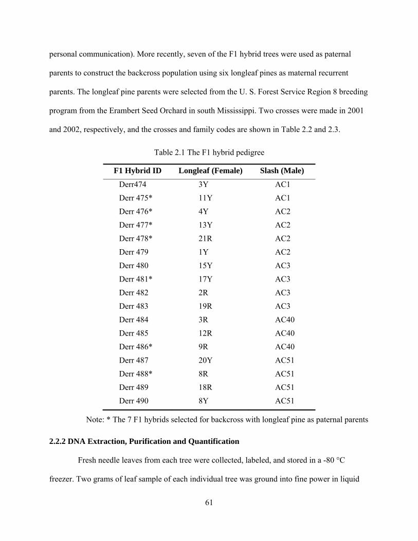
61
personal communication). More recently, seven of the F1 hybrid trees were used as paternal
parents to construct the backcross population using six longleaf pines as maternal recurrent
parents. The longleaf pine parents were selected from the U. S. Forest Service Region 8 breeding
program from the Erambert Seed Orchard in south Mississippi. Two crosses were made in 2001
and 2002, respectively, and the crosses and family codes are shown in Table 2.2 and 2.3.
Table 2.1 The F1 hybrid pedigree
F1 Hybrid ID Longleaf (Female) Slash (Male)
Derr474 3Y AC1
Derr 475* 11Y AC1
Derr 476* 4Y AC2
Derr 477* 13Y AC2
Derr 478* 21R AC2
Derr 479 1Y AC2
Derr 480 15Y AC3
Derr 481* 17Y AC3
Derr 482 2R AC3
Derr 483 19R AC3
Derr 484 3R AC40
Derr 485 12R AC40
Derr 486* 9R AC40
Derr 487 20Y AC51
Derr 488* 8R AC51
Derr 489 18R AC51
Derr 490 8Y AC51
Note: * The 7 F1 hybrids selected for backcross with longleaf pine as paternal parents
2.2.2 DNA Extraction, Purification and Quantification
Fresh needle leaves from each tree were collected, labeled, and stored in a -80 °C
freezer. Two grams of leaf sample of each individual tree was ground into fine power in liquid

62
Table 2.2 The pedigree and backcross code for crosses made in 2001
CrossCode Female (longleaf) Male (hybrid) Test Group
1 Em04 Derr488 488_1
2 Em14 Derr488 488_1
3 Em17 Derr488 488_1
4 Em24 Derr488 488_1
5 Em41 Derr488 488_1
6 Em45 Derr488 488_1
7 Em04xwind
8 Em04 Derr475 FT_1
9 Em04 Derr476 FT_1
10 Em04 Derr477 FT_1
11 Em04 Derr478 FT_1
12 Em04 Derr481 FT_1
13 Em04 Derr486 FT_1
14 Slash Control
15 Longleaf Control
Table 2.3 The pedigree and backcross code for crosses made in 2002
Female Parents
Male Parents Em04 Em14 Em17 Em24 Em41 Em45
Derr475 fam1 fam9 fam18 fam26 fam39 fam34
Derr476 fam2 fam10 fam19 fam27 fam40 n/a
Derr477 fam3 fam11 fam20 fam28 fam41 fam35
Derr478 fam4 fam12 n/a* fam29 fam42 fam36
Derr481 fam5 fam13 fam22 fam30 fam43 fam37
Derr486 fam6 fam14 fam23 fam31 fam44 fam38
Derr488 fam7 fam15 fam24 fam32 n/a n/a
* There are no offspring available for these families.
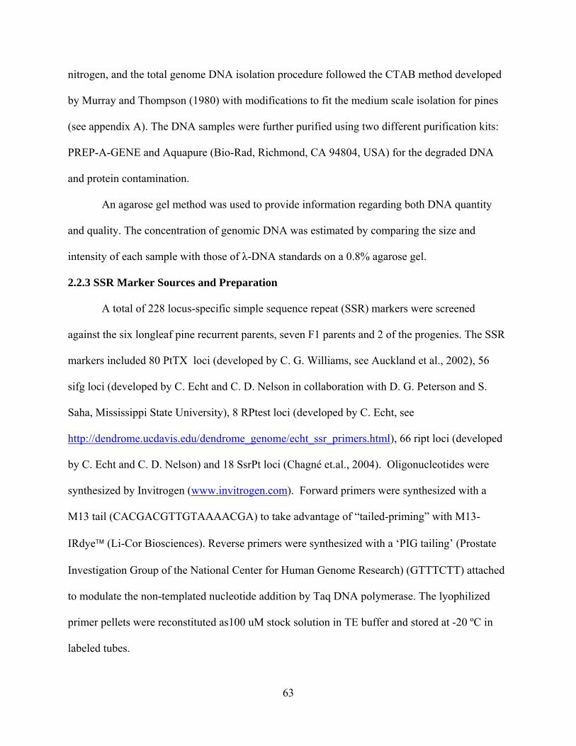
63
nitrogen, and the total genome DNA isolation procedure followed the CTAB method developed
by Murray and Thompson (1980) with modifications to fit the medium scale isolation for pines
(see appendix A). The DNA samples were further purified using two different purification kits:
PREP-A-GENE and Aquapure (Bio-Rad, Richmond, CA 94804, USA) for the degraded DNA
and protein contamination.
An agarose gel method was used to provide information regarding both DNA quantity
and quality. The concentration of genomic DNA was estimated by comparing the size and
intensity of each sample with those of λ-DNA standards on a 0.8% agarose gel.
2.2.3 SSR Marker Sources and Preparation
A total of 228 locus-specific simple sequence repeat (SSR) markers were screened
against the six longleaf pine recurrent parents, seven F1 parents and 2 of the progenies. The SSR
markers included 80 PtTX loci (developed by C. G. Williams, see Auckland et al., 2002), 56
sifg loci (developed by C. Echt and C. D. Nelson in collaboration with D. G. Peterson and S.
Saha, Mississippi State University), 8 RPtest loci (developed by C. Echt, see
http://dendrome.ucdavis.edu/dendrome_genome/echt_ssr_primers.html), 66 ript loci (developed
by C. Echt and C. D. Nelson) and 18 SsrPt loci (Chagné et.al., 2004). Oligonucleotides were
synthesized by Invitrogen (www.invitrogen.com). Forward primers were synthesized with a
M13 tail (CACGACGTTGTAAAACGA) to take advantage of “tailed-priming” with M13-
IRdye™ (Li-Cor Biosciences). Reverse primers were synthesized with a ‘PIG tailing’ (Prostate
Investigation Group of the National Center for Human Genome Research) (GTTTCTT) attached
to modulate the non-templated nucleotide addition by Taq DNA polymerase. The lyophilized
primer pellets were reconstituted as100 uM stock solution in TE buffer and stored at -20 ºC in
labeled tubes.

64
2.2.4 Preliminary Testing and Optimization of PCR Reaction Conditions
Before proceeding to detailed evaluation of the markers, the primers were verified to
amplify the desired region successfully from genomic DNA, and the optimal reaction condition
for PCR amplification was also determined. For each primer pair to be tested, I prepared a 10 ul
reaction mixture, 2 ul 5x reaction buffer, 20 ng genomic DNA (3.2 ul x 6.25 ng/ul), 100 nM each
primer pair, 1 unit of Taq DNA polymerase in storage buffer B (20mM Tris-HCl, pH 8.0 at 25ºC,
100 mM KCl, 0.1 mM EDTA, 1 mM DTT, 50% glycerol , 0.5% Tween20 and 0.5% Nonidet-
P40, Promega) or 0.25 unit GoTaq Flexi DNA polymerase (Promega), 100 nM dNTP solution,
and corresponding distilled water. A factorial design was used to test the different MgCl2
concentrations (1.5 uM, 2.0 uM, 2.5 uM , 3.0 uM, 3.5 uM, 4.0 uM and 4.5 uM) and touchdown
temperature profiles (50 °C, 55 °C, 60 °C, and 65 °C). The PCR reaction cycle started with a hot
start at 95 °C for 4 min, followed by a touchdown series of cycles with different initial annealing
temperatures for each marker (i.e., primer pair) and decreasing by 0.5 °C per cycle for 20 cycles,
followed by 20 cycles at the final annealing temperature, and ending with a 15 min extension at
72 °C. After the PCR reaction, 4 uL blue stop solution (Bromophenol Blue, 95% Formamide, Li-
Cor) were added to each of the reaction mixes. The thermcycles used were 96 wells PTC-100 TM
programmable thermal controllers (M.J. Research Inc.).
Electrophoresis was conducted on an automatic DNA sequencer (Li-cor 4200 series DNA
sequencer). Amplified DNA fragments were separated on a 6% denaturing polyacrylamide gel
mix (Li-Cor). The gels were cast at least 90 minutes before use and pre-run for 30 min just
before loading the samples. Pre-running and running electrophoresis steps were performed using
16-bit data collection, 1500 V, 40 W, 40 mA, 45 °C, and 4 X scan speed as recommended by Li-
Cor. The 1X TBE (89 mM Tris, 89 mM borate, 2.2 mM EDTA pH 8.3) was used as the running
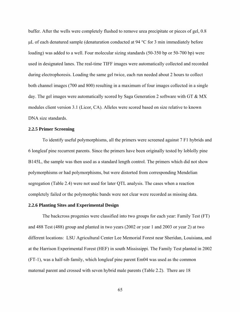
65
buffer. After the wells were completely flushed to remove urea precipitate or pieces of gel, 0.8
μL of each denatured sample (denaturation conducted at 94 °C for 3 min immediately before
loading) was added to a well. Four molecular sizing standards (50-350 bp or 50-700 bp) were
used in designated lanes. The real-time TIFF images were automatically collected and recorded
during electrophoresis. Loading the same gel twice, each run needed about 2 hours to collect
both channel images (700 and 800) resulting in a maximum of four images collected in a single
day. The gel images were automatically scored by Saga Generation 2 software with GT & MX
modules client version 3.1 (Licor, CA). Alleles were scored based on size relative to known
DNA size standards.
2.2.5 Primer Screening
To identify useful polymorphisms, all the primers were screened against 7 F1 hybrids and
6 longleaf pine recurrent parents. Since the primers have been originally tested by loblolly pine
B145L, the sample was then used as a standard length control. The primers which did not show
polymorphisms or had polymorphisms, but were distorted from corresponding Mendelian
segregation (Table 2.4) were not used for later QTL analysis. The cases when a reaction
completely failed or the polymorphic bands were not clear were recorded as missing data.
2.2.6 Planting Sites and Experimental Design
The backcross progenies were classified into two groups for each year: Family Test (FT)
and 488 Test (488) group and planted in two years (2002 or year 1 and 2003 or year 2) at two
different locations: LSU Agricultural Center Lee Memorial Forest near Sheridan, Louisiana, and
at the Harrison Experimental Forest (HEF) in south Mississippi. The Family Test planted in 2002
(FT-1), was a half-sib family, which longleaf pine parent Em04 was used as the common
maternal parent and crossed with seven hybrid male parents (Table 2.2). There are 18

66
Table 2.4 Possible marker genotype combinations and segregation pattern
Parents Offspring
CrossType Cross P1 P2
ObservedBand
Informa-tiveness*
Observed Band
Segregation No. Phenotype
A 1 ab×cd ab×cd FI ac ad bc bd 1:1:1:1 4 2 ab×ac ab×ac FI a ac ba bc 1:1:1:1 4 3 ab×co ab×c FI ac a bc b 1:1:1:1 4 4 ao×bo a×a FI ab a b o 1:1:1:1 4 B B1 5 ab×ao ab×a BI ab 2a b 1:2:1 3 B2 6 ao×ab a×ab BI ab 2a b 1:2:1 3 B3 7 ab×ab ab×ab BI a 2ab b 1:2:1 3 C 8 ao×ao a×a BI 3a o 3:1 2 D D1 9 ab×cc ab×c MI ac bc 1:1 2 10 ab×aa ab×a MI a ab 1:1 2 11 ab×oo ab×o MI a b 1:1 2 12 bo×aa b×a MI ab a 1:1 2 13 ao×oo a×o MI a o 1:1 2 D2 14 cc×ab c×ab PI ac bc 1:1 2 15 aa×ab a×ab PI a ab 1:1 2 16 oo×ab o×ab PI a b 1:1 2 17 aa×bo a×b PI ab a 1:1 2 18 oo×ao o×a PI a o 1:1 2 E 19 aa×bb a×b NI ab 1 1 20 aa×aa a×a NI a 1 1
Table source: Wu (2002) with minor modifications. Cross: o: null allele *Informativeness: FI: Full information for both maternal and paternal parents (multiple alleles per locus); BI: Informative for both maternal and paternal parents (two alleles per locus); MI: Informative for the maternal parent; PI: Informative for the paternal parent; NI: Not informative

67
replications in a RCB Design in each location and 1 plant per cross (15 plants) in each
replication. For the Family Test planted in 2003 (FT-2), it included all available 38 full-sib
backcross families (Table 2.3). There are 6 replications and 30 crosses in each replication with 6
trees planted in the same row per cross. The progenies of 488 test came from a half-sib family
where hybrid male parent Derr488 served as the common paternal parents and crossed with six
female longleaf parents and followed a completely randomized design (CRD) in both locations
and years. However, the 488 test planted in 2003 (488-2) was not replicated in Louisiana.
2.2.7 Field Data Collection
The total height and diameter values were used to address the EHG of the longleaf
backcross population. The total height was scored as the height from the ground to the top of the
stem. The diameter measurement had three values: the first diameter measurement (d3) was
scored as the ground level diameter; the second diameter measurement (d4) was scored as the 15
cm level diameter above the ground; the third diameter measurement (d5) was scored as the 30
cm level diameter above the ground. For these seedlings planted in 2002, four height
measurements, ht2, ht3, ht4, and ht5, and three diameter measurements, d3, d4, and d5 were
taken in 2004, 2005, 2006, and 2007. For the trees planted in 2003, three height measurements,
ht2, ht3, and ht4 and two diameter measurements, d3 and d4, were taken in 2005, 2006, and 2007,
respectively (see Table 2.5 for detailed variable information).
Table 2.5 The response variables used in data analyses
Year measured Trees planted in 2002 Trees planted in 2003 Jan, 2004 ht2 Feb, 2005 ht3 d3 ht2 Jan, 2006 ht4 d4 ht3 d3 Dec, 2006 ht5 d5 ht4 d4

68
2.2.8 Statistical Analyses in Genetic Variance Estimation
The variance component estimation was followed by the method of Wu and Stettler
(1997). Data analyses were based on analyses of variance (ANOVA) with SAS procedure PROC
MIXED. The effects of Location, Parent, Parent x Location, Replication within Location and
Parent x Replication within Location for each male or female parent were estimated. However,
tests of main effect were confounded by the effects of interaction, making it difficult to
conclusively determine the significance and variance components of main effects. To solve the
problem, the parent x location interaction was first tested. If the interaction was not significant,
the variance component for parents can be estimated by the model directly. If the interaction was
significant, the residual variance, which included the genetic variance component and the
specific-site environment, would be used. The variance components for the effects were
calculated by equating the mean squares with the expected mean squares derived from type III
sums of squares.
Two different statistical models were used to estimate the variance component. Since
there were multiple measurements for both height and diameter, in the first method, each height
or diameter measurement was treated as an individual response variable, thus 7 separate
ANOVA analyses for all the measurements were conducted in this model. The second model
treated all the height or diameter measurements as repeat measurements, and only two analyses
were conducted for the height and diameter as response variables, respectively.
The statistical model for the first method:
2.1
where was the different height or diameter value for the ith parent, jth location, kth replication,
and lth tree. was overall mean, was for the male or female effect (i=1, 2…7 for male parent

69
and i=1, 2,…,6 for female parent), was for location effect (i=1, 2 Louisiana or Mississippi),
was for the replication, and ε was for residual error term. The male and female effects were
analyzed separately because they were not strictly 2-way factorial designs due to availability of
the seeds.
The second model was a repeated measurement, that is, the height or diameter in different
years were treated as one single response variable, and the time of measurement was used as a
time serial variable. The statistical model for the method 2 was:
2.2
where was the height or diameter measurement, is overall mean, was for the male or
female effect (i=1, 2…7 for male parent and i=1, 2…6 for female parent), was for location
effect (i=1, 2 Louisiana or Mississippi), was the repeat measurement for each height and
diameter value (m=1, 2, 3 for height measurements and m=1, 2 for diameter measurements), and
ε was the residual error term.
2.3 Results and Discussion
2.3.1 Finding the Optimal Condition for PCR Amplification of SSRs
The ‘PIG tailing’ (5’-GTTTCTT-3’) was very efficient for minimizing the effects of
enzyme-directed, template-independent additions of an “A” nucleotide to PCR amplification by
DNA polymerase. It has shown that the stuttered bands were reduced and the band patterns were
clean and uniform (Figure 2.1), which can reduce genotype error significantly, especially for
automatic genotyping by software which only read the band signal. Tailing the primers has also
allowed altering magnesium concentrations to reduce the noise and increase band signal.
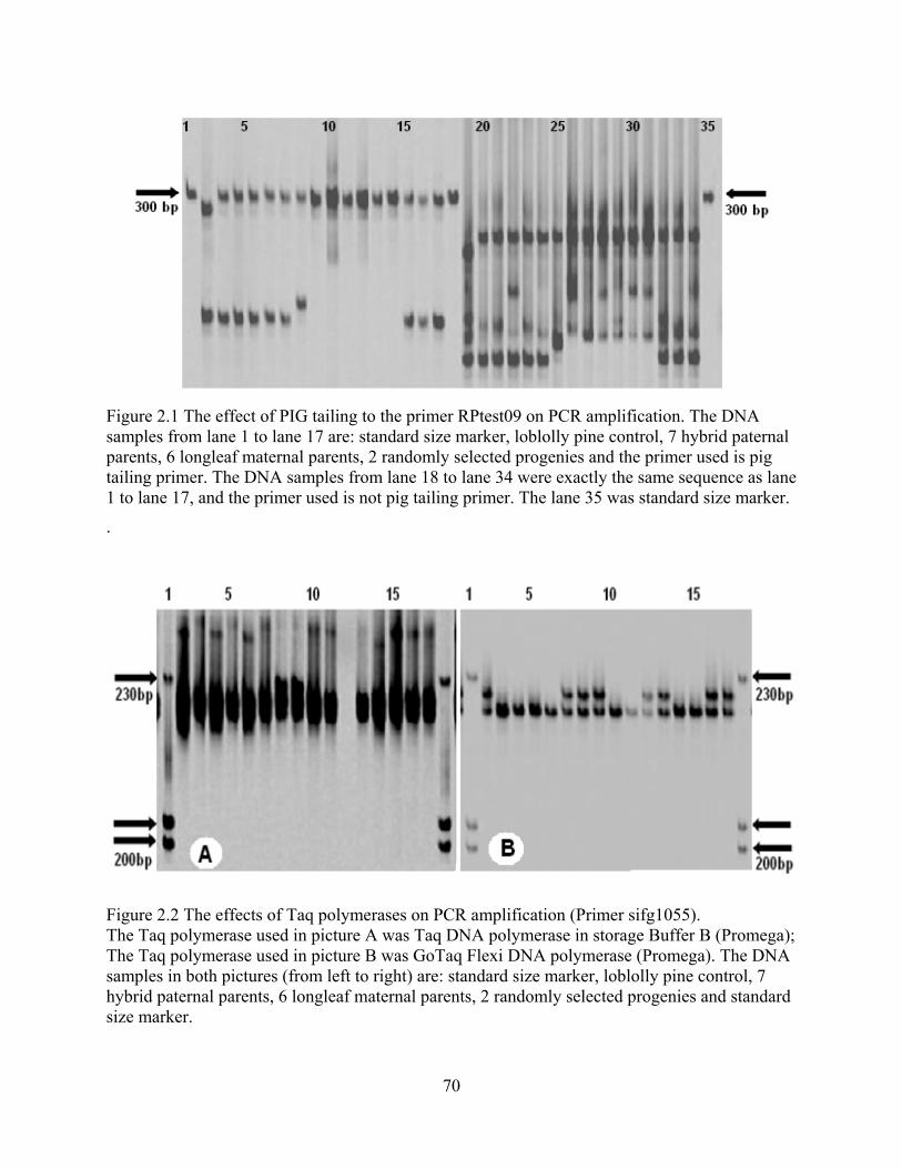
70
Figure 2.1 The effect of PIG tailing to the primer RPtest09 on PCR amplification. The DNA samples from lane 1 to lane 17 are: standard size marker, loblolly pine control, 7 hybrid paternal parents, 6 longleaf maternal parents, 2 randomly selected progenies and the primer used is pig tailing primer. The DNA samples from lane 18 to lane 34 were exactly the same sequence as lane 1 to lane 17, and the primer used is not pig tailing primer. The lane 35 was standard size marker.
.
Figure 2.2 The effects of Taq polymerases on PCR amplification (Primer sifg1055). The Taq polymerase used in picture A was Taq DNA polymerase in storage Buffer B (Promega); The Taq polymerase used in picture B was GoTaq Flexi DNA polymerase (Promega). The DNA samples in both pictures (from left to right) are: standard size marker, loblolly pine control, 7 hybrid paternal parents, 6 longleaf maternal parents, 2 randomly selected progenies and standard size marker.

71
Taq DNA polymerase used less amounts of DNA polymerase, less magnesium, and
produced more uniform and clean amplification (see Figure 2.2). With the new DNA
polymerase, 18 primers that failed amplifying or amplified but could not be genotyped have
shown perfect polymorphisms. This outcome is probably due to the high glycerol concentration
in the stock solution associated with a high concentration of polymerase, resulting in an
unbalanced amplification of various loci and a slight increase in the background.
For optimizing the PCR condition, the first step was to determine the concentration of the
DNA template. Based on the preliminary test, a DNA concentration of 20 ng was chosen for
future amplification. Keeping all other parameters fixed the effects of MgCl2 concentration and
initial annealing temperatures were also investigated. These two factors can affect the
amplification in different ways for different sources of the primers (Figure 2.3 and Figure 2.4).
Since Mg2+ ions form complexes with dNTPs, primers, and DNA templates, the concentration of
MgCl2 was assumed to be the component with the most dramatic effects on specificity. Thus, the
optimal concentration of MgCl2 has to be selected for each experiment. Too few Mg2+ ions result
in a low yield of PCR product, and too many ions increase the yield of non-specific products and
promote misincorporation. In our experiments, with the new GoTaq Flexi DNA polymerase,
MgCl2 concentration ranges of 2.5±0.5 mM are suitable in most cases.
The optimal initial annealing temperature depends upon the melting temperature of the
primer-template hybrid. If the temperature is too high, the primers will not anneal efficiently, and
if the annealing temperature is too low, the primers may anneal nonspecifically. Usually, the
optimal annealing temperature is 5°C lower than the melting temperature of the primer-template
DNA duplex. Incubation for 0.5-2 minutes is usually sufficient. However, if nonspecific PCR
products are obtained in addition to the expected product, the annealing temperature should be

72
optimized by increasing it stepwise by 1-2°C. In our experiment, with the new GoTaq Flexi
DNA polymerase and optimized MgCl2 concentration, an initial annealing temperature of 60 °C
was suitable for the majority of the primer pairs. The optimized PCR reaction conditions for all
228 polymorphic markers were obtained. These optimized PCR reaction condition profiles
would facilitate the later marker screen and genotyping.
Figure 2.3 The effect of Mg2+ on PCR amplification (Primer: PtTX_3117). Picture A was for Mg2+ = 1.5 mM and picture B was 2.5 mM. The initial annealing temperature was 60 ºC. The DNA samples for picture A were (from left to right): standard size marker, loblolly control, 7 paternal parents. The DNA samples for picture B were (from left to right): 6 longleaf maternal parents, 2 randomly selected progenies and standard size marker.
Figure 2.4 The effect of initial annealing temperature on PCR amplification (PtTX_3116). Picture A was for temperature at 50 ºC and picture B was for 60 ºC. The DNA samples for picture A were (from left to right): standard size marker, loblolly control, 7 paternal parents. The DNA samples for picture B were (from left to right): 6 longleaf maternal parents, 2 randomly selected progenies and standard size marker.
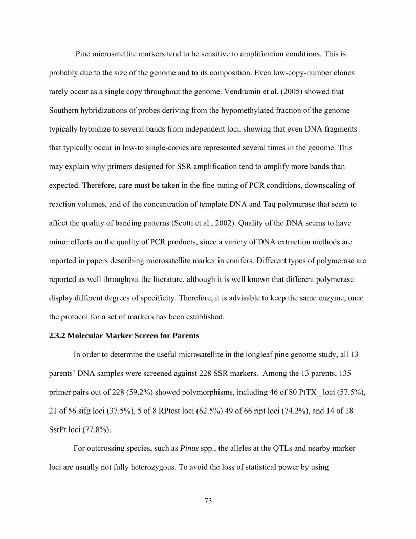
73
Pine microsatellite markers tend to be sensitive to amplification conditions. This is
probably due to the size of the genome and to its composition. Even low-copy-number clones
rarely occur as a single copy throughout the genome. Vendramin et al. (2005) showed that
Southern hybridizations of probes deriving from the hypomethylated fraction of the genome
typically hybridize to several bands from independent loci, showing that even DNA fragments
that typically occur in low-to single-copies are represented several times in the genome. This
may explain why primers designed for SSR amplification tend to amplify more bands than
expected. Therefore, care must be taken in the fine-tuning of PCR conditions, downscaling of
reaction volumes, and of the concentration of template DNA and Taq polymerase that seem to
affect the quality of banding patterns (Scotti et al., 2002). Quality of the DNA seems to have
minor effects on the quality of PCR products, since a variety of DNA extraction methods are
reported in papers describing microsatellite marker in conifers. Different types of polymerase are
reported as well throughout the literature, although it is well known that different polymerase
display different degrees of specificity. Therefore, it is advisable to keep the same enzyme, once
the protocol for a set of markers has been established.
2.3.2 Molecular Marker Screen for Parents
In order to determine the useful microsatellite in the longleaf pine genome study, all 13
parents’ DNA samples were screened against 228 SSR markers. Among the 13 parents, 135
primer pairs out of 228 (59.2%) showed polymorphisms, including 46 of 80 PtTX_ loci (57.5%),
21 of 56 sifg loci (37.5%), 5 of 8 RPtest loci (62.5%) 49 of 66 ript loci (74.2%), and 14 of 18
SsrPt loci (77.8%).
For outcrossing species, such as Pinus spp., the alleles at the QTLs and nearby marker
loci are usually not fully heterozygous. To avoid the loss of statistical power by using

74
homozygous individual parents for the mapping population, all parents and families were
evaluated for their heterozygosity and number of informative polymorphic markers. The
polymorphic marker information for each parent is listed in Table 2.6.
Table 2.6 Summary of polymorphic markers that generate different loci information among parents
Table 2.7 Number of informative polymorphic SSR markers within each family
Cross Family size TI FI BI PI MI NI
Em04xDerr488 274 104 27 7 43 27 31
Em14xDerr488 249 99 21 10 48 20 36
Em17xDerr488 150 102 34 10 34 24 33
Em24xDerr488 364 103 28 17 35 23 32
Em41xDerr488 110 104 29 13 38 24 31
Em45xDerr488 61 109 23 13 44 29 26
FI: # full informative markers; BI: # both maternal and paternal informative markers; PI: # paternal informative markers; MI: # maternal informative markers; NI: # non informative markers; TI: total number of informative markers.
Parent Species Homozygous loci Heterozygous loci Non amplification
Derr475 F1 55 76 (56%) 4
Derr476 F1 57 72 ( 53%) 6
Derr477 F1 68 60 (44%) 7
Derr478 F1 57 69 (51%) 9
Derr481 F1 58 70 (52%) 7
Derr486 F1 60 68 (47%) 7
Derr488 F1 54 80 (59%) 1
Em04 Longleaf 66 65 (48%) 4
Em14 Longleaf 70 56 (41%) 9
Em17 Longleaf 61 70 (46%) 4
Em24 Longleaf 58 68 (50%) 9
Em41 Longleaf 66 66 (49%) 3
Em45 Longleaf 66 65 (48%) 4

75
For the male parents, Derr488 showed the highest ratio of heterozygous loci, least
frequency of non-amplification and largest population size which indicated the parent was a
potential candidate for parent selection on mapping purpose. Therefore, the number of
informative markers within each full-sib family of Derr488 half-sib family was evaluated and the
results were listed in Table 2.7.
2.3.3 Genetic Variance Estimation
It is expected that the more the parental lines differ, the more genetic factors will be
described for the trait in the segregating population and the easier the identification. However,
the height growth data for both grandparents and parents were not available, and the information
has to be inferred by the phenotypic and genetic variation in backcross population. The
phenotypic variation is determined by the genetic variation, environmental variation and their
interaction. The broad sense heritability is characterized by the genetic variation portion in the
whole phenotypic variation. I want to maximize the genetic variation part, thus the parents that
have large phenotypic variation but small heritability are not favorable.
The main effects of parent, location, and the interaction between parent x location effects
were tested first, and the test probability for each response variable was plotted in Figure 2.5. If a
test effect was not significant, then it could be omitted from the full model. All the male and
female effects were highly significant. The location effect was not significant for both male and
female effects, except at the Ht2 variable. For the interaction effect, the female x location effect
was not significant at ht2 and ht3, while the male x location effect was not significant at D3.
However, for method 2, all the effects were significant.
According to the above results, the new reduced model for each height or diameter
variables was created, and the observation number (N), mean (M), and genetic variance
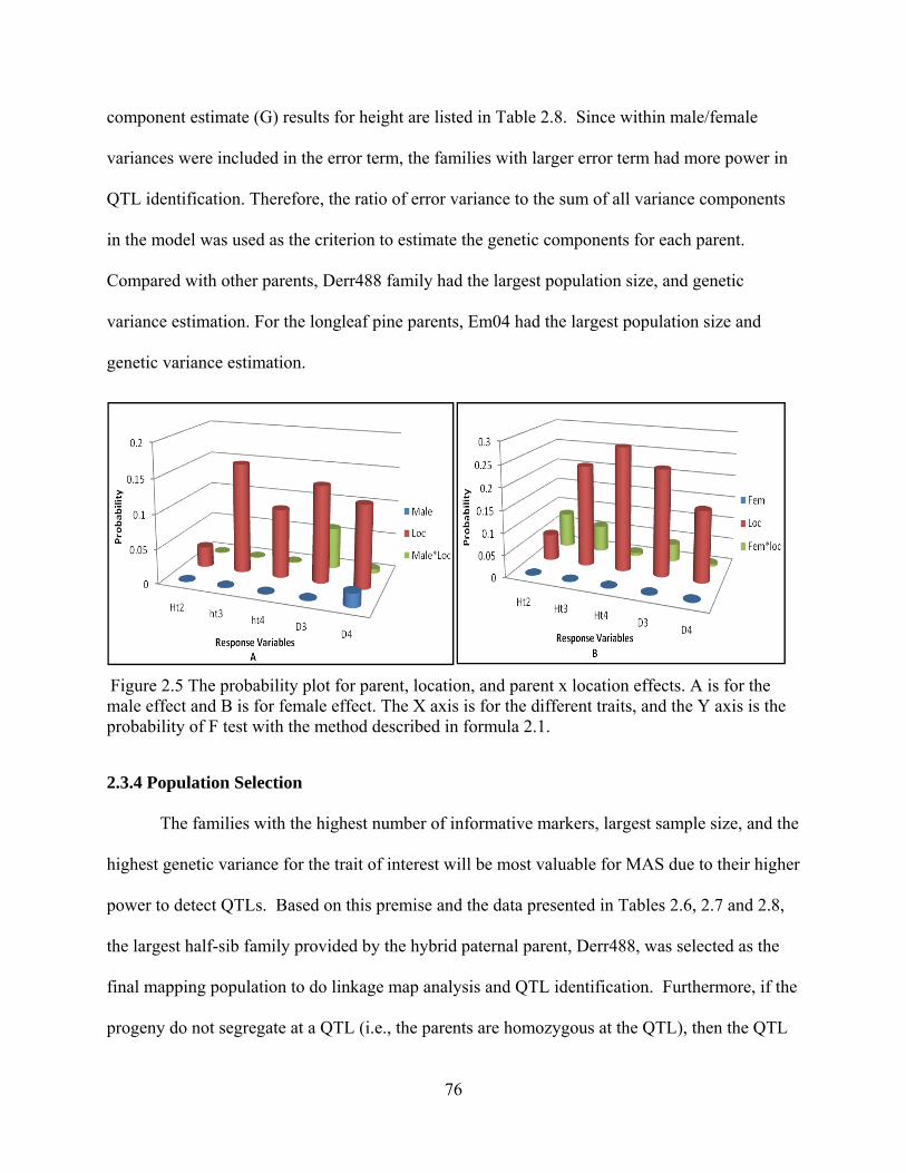
76
component estimate (G) results for height are listed in Table 2.8. Since within male/female
variances were included in the error term, the families with larger error term had more power in
QTL identification. Therefore, the ratio of error variance to the sum of all variance components
in the model was used as the criterion to estimate the genetic components for each parent.
Compared with other parents, Derr488 family had the largest population size, and genetic
variance estimation. For the longleaf pine parents, Em04 had the largest population size and
genetic variance estimation.
Figure 2.5 The probability plot for parent, location, and parent x location effects. A is for the male effect and B is for female effect. The X axis is for the different traits, and the Y axis is the probability of F test with the method described in formula 2.1.
2.3.4 Population Selection
The families with the highest number of informative markers, largest sample size, and the
highest genetic variance for the trait of interest will be most valuable for MAS due to their higher
power to detect QTLs. Based on this premise and the data presented in Tables 2.6, 2.7 and 2.8,
the largest half-sib family provided by the hybrid paternal parent, Derr488, was selected as the
final mapping population to do linkage map analysis and QTL identification. Furthermore, if the
progeny do not segregate at a QTL (i.e., the parents are homozygous at the QTL), then the QTL

77
cannot be detected. Muranty (1996) showed that a mating design with six parents will allow a
reasonable power for QTL detection if QTL heterzogosity frequency in the base population is at
least 0.2. This result adds support to the decision to select the half-sib family with common
paternal parent Derr488 and six different longleaf pine maternal parents to identify QTLs
controlling EHG in the study.
Table 2.8 Genetic variance estimation results for Height variables from two different methods
Method I Method II
Parents
ht2 ht3 ht4 Repeat
N M G (%) N M G (%) N M G (%) G (%)
Derr475 281 34 77 273 104 74 257 187 59 63
Derr476 168 28 73 165 92 70 156 170 65 55
Derr477 157 32 75 148 101 64 141 174 46 45
Derr478 265 30 70 250 49 58 240 177 54 52
Derr481 428 23 57 417 88 74 408 169 70 63
Derr486 256 27 79 254 90 75 251 160 64 34
Derr488 1257 27 71 1243 90 76 1208 184 81 65
Ctl(LL) 31 14 20 31 42 17 31 130 79 32
Ctl(Sl) 11 95 89 11 159 92 11 272 84 67
Em04 936 25 87 924 90 83 897 172 63 65
Em14 669 22 59 643 79 65 626 156 56 53
Em17 241 28 36 237 98 56 231 194 49 57
Em24 777 32 47 764 103 72 738 193 52 68
Em41 241 27 68 239 83 62 227 170 38 47
Em45 217 27 70 214 87 70 210 169 37 43
Method I: Ht: height. Each height variable was treated as a separate dependent variable in the model. N: Total number of the observation for the family. M: the mean estimation for the family. G: Genetic component: the ratio of residual to the sum of all variance components in the model, used to estimate within parent variance; Method II: The height variable was treated as repeat measurements. Ctl (LL): Longleaf pine control. Ctl (SL): Slash pine control.

78
2.3.5 Selective Genotyping
A half-sib family with Derr488 as the common paternal parents was selected as the final
mapping population for this study. There are more than 1200 samples in this half-sib family, and
it was impossible to genotype all these progenies. Random selection has always been a good way
to do the unbiased estimation, however, in this study, a procedure termed ‘selective genotyping’
(Darvasi and Soller, 1992; Lander and Botstein 1989; Lebowitz et al., 1987) was used. With this
method, only individuals from the high and low phenotypic extremes were genotyped. The major
limitation of this approach is that if the aim of the experiment is analyzing a set of traits,
selecting the extremes of each trait one would select most of the population, and then no
reduction in genotyping can be obtained. Selective genotyping is the most appropriate for the
cases where only one trait is being analyzed. In this case, the height growth and diameter were
highly correlated (results will be showed in Chapter 5), thus the SG was appropriate for the
purpose of this study.
A two-step sample selection strategy was used in our research: Within each of the six
full-sib families, the tallest and shortest 8 percent of seedlings (220 seedlings total) were selected
for QTL detection (phase I). Random selections of 8 percent of the seedlings from the rest of the
population (110 seedlings) and 10 seedlings from both tails (130 seedlings total) of the within-
family distributions will be used for unbiased QTL verification and mapping (phase II).
2.5 References
Auckland, L.D., Bui, T., Zhou, Y., Shepherd, M. and Williams, C.G. 2002. Conifer microsatellite handbook. College Station, TX USA: Texas A & M. pp26.
Barreneche, T., Casasoli, M., Russell, K., Akkak, A., Meddour, H., Plomion, C., Willani, F., Kremer, A. 2004. Comarative mapping between Quercus and Castanea using simple-sequence repeats (SSRs). Theor. Appl. Genet. 108: 558-566.
79
Beckmann, J.S. and Soller, M. 1990. Toward a unified approach to the genetic mapping of eukaryotes based on sequence-tagged microsatellite sites. Biotechnology 8: 930–932.
Bennett, M.D., Leitch, I.J. 2003. Plant DNA C-values database Release 2.0. http://www.rbgkew.org.uk/cval/homepage.html.
Bostein, D., White, R.L., Skolnick, M., and Davis, R. W. 1980. Construction of a genetic linkage maps in man using restriction fragment length polymorphisms. Amer. J. Hum. Genet. 32:314-331.
Brondani, R.P., Brondani, C., Tarchini, R.L., Grattapaglia, D. 1998. Development, characterization and mapping of microsatellite markers in Eucalyptus grandis and E. urophylla. Theor. Appl. Genet. 97: 816-827.
Brown, C.L., 1964. The seedling habit of longleaf pine. Athens, GA: Georgia Forest Research Council and the University of Georgia, School of Forestry.
Brownstein, M.J., Carpten, J.D, Smith, J.R. 1996. Modulation of Non-Templated Nucleotide Addition by Taq DNA Polymerase: Primer Modifications that Facilitate Genotyping. Biotechniques 20: 1004-1010.
Byrne, M., Marquez-Garcia, M.I., Uren, T., Smith, D.S. Moran, G.F. 1996. Conservation of genetic diversity of microsatellite loci in the genus Eualyptus. Aust. J. Botany 44: 331-341.
Chagné, D., Chaumeil, P., Ramboer, A., Collada, C., Guevara, A., Cervera, M.T., Vendramin, G.G., Garcia, V., Frigerio, J-M., Echt, C., Richardson, T., Plomion, C., 2004. Cross-species transferability and mapping of genomic and cDNA SSRs in pines. Theor. Appl. Genet. 109: 1204-1214.
Decroocq, S., Butcher, P.A, Moran, G.F., 1997. Genetic Diversity and conservation of microsatellite loci in acacias. Poster presented at Plant and Animal Genome V conference, San Diego, California, Jan. 12-17.
Derr, H.J, 1966. Longleaf ×slash pine hybrids at age 7: survival, growth, and disease susceptibility. J For. 64: 236–239.
Dettori, M.T., Quarta, R., Verde, I. 2001. A peach linkage map integrating RFLPs, SSRs, RAPDs, and morphological markers. Genome 44: 783–790.
Devey M.E, Bell, J.C., Uren, T.L, Moran, G.F. 2002. A set of microsatellite markers for fingerprinting and breeding applications in Pinus radiata. Genome 45: 984-989.
Echt, C.S., Nelson, C.D. 1997. Linkage mapping and genome length in eastern white pine (Pinus strobus L.). Theor. Appl. Genet. 94: 1031-1037.
Echt, C.S., Vendramin, G.G., Nelson, C.D., Marquardt, P. 1999. Microsatellite DNA as shared genetic markers among conifer species. Can. J. For. Res. 29: 365-371.

80
Elsik, C.G., Williams, C.G. 2000. Retroelements contribute to the excess low-copy number DNA in pine. Mol. Gen. Genet. 264: 47-55.
Elsik, C.G. Williams, C.G. 2001. Low-copy microsatellite recovery from a conifer genome. Theor. Appl. Genet. 103: 1189-1195.
Fisher, P.J., Gardner, R.C., Richardson, T.E., 1996. Single locus microsatellite isolated using 5’ anchored PCR. Nuc. Acid. Res. 24: 4369-4371.
Fisher, P.J., Richardson, T.E. Gardner, R.C., 1998. Characteristics of single- and multi-copy microsatellites from Pinus Radiata. Theor. Appl. Genet. 96: 969-979.
Gillet, E.M. 1999. Which marker for which purpose? Final compendium of the research project “Development, Optimization and Validation of Molecular Tools for Assessment of Biodiversity in Forest Trees”. In: European Union DGXII Biotechnology FW IV Research Programme “Molecular Tools for Biodiversity.” Http://www.webdoc.gwdg.de/ebook/y/1999/whichmarker/cmarker.htm.
Glaubitz, J.C., Strk, J., Moran, G.F. 1999. Genetic impacts of different silvicultural practices in native eucalypt forests. In: Forest Genetics and Sustainbility. Edited by Matyas, C., Kluwer, D. the Netherlands.
Guevara, M.A., Chagné, D., Almeida, M.H., Byrne, M., Collada, C., Favre, J.M., Harvengt, L., Jeandroz, S., Orazio, C., Plomion, C., Ramboer, A., Rocheta, M., Sebastiani, F., Soto, A., Vendramin, G.G., Cervera, M.T. 2005. Isolation and characterization of nuclear microsatellite loci in Pinus pinaster Ait. Mol. Ecol. Notes 5: 57-59.
Hearne, C.M., Ghosh, S., Todd, J.A. 1992. Microsatellites for linkage analysis of genetic traits. Trends Genet. 8: 288–294.
Hutchison, K., Singer, P., Volkaert, H., Deker, A., Costello, L., Greenwood, M., 1994. A PCR-based molecular genetic map for the conifer Larix Decidua. The International Conference on the Plant Genome II 24-27 January. San Diego, CA poster #90.
Joobeur, T., Periam, N., de Vicente, M.C., King, G.J., Arffls, P. 2000. Development of a second-generation linkage map for almond using RAPD and SSR markers. Genome 43: 649–655.
Karhu A., Dieterich J.H., Savolainen, O. 2000. Rapid expansion of microsatellite sequences in pines. Mol. Biol. Evol. 17: 259–265.
Kriebel, H.B., 1985. DNA sequence components in the Pinus Strobus nuclear genome. Can. J. For. Res.15: 1-4.
Layton, P.A., Goddard, R.E., 1982. Environmental and genetics effects on the duration of the grass-stage in longleaf pine. In: Proceeding of the Seventh North American Forest Biology Workshop, Lexington, KY, July 26-28, 1982 Lexington, KYL University of Kentycky: pp131-136.
81
Leitch, I.J., Hanson, L., Winfield, M., Parker, J., Bennett, M.D. 2001. Nuclear DNA C-values complete familial representation in Gymnosperms. Ann. Bot. 88: 843-849.
Levinson, G., Gutman, G.A. 1987. Slipped-strand mispairing: a major mechanism for DNA sequence evolution. Mol. Biol. Evol. 4: 203–221.
Lian, C., Oishi, R., Miyashita, N., Hogetsu, T., 2004. High somatic instability of a microsatellite locus in a clonal tree, Robinia pseudoacacia. Theor. Appl. Genet. 108: 836–841.
Liebhard, R., Gianfranceschi, L., Koller, B., Ryder, C.D., Tarchini, R., Van De Weg, E., Gessler, C. 2002. Development and characterization of 140 new microsatellites in apple (Malus domestica Borkh.). Mol. Breed. 10: 217–241.
Liepelt, S., Kuhlenkamp, V., Anzidei, M., Vendramin, C.G., and Ziegenhagen, B. 2001. Pitfalls in determining size homoplasy of microsatellite loci. Mol. Ecol. Notes 1: 332-335.
Mariette, S., Chagné, D., Decroocq, S., Vendramin, G.G., Lalanne, C., Madur, C., Plomion, C. 2001. Microsatellite markers for Pinus pinaster Ait. Ann. For. Sci. 58: 203-206.
Marquardt, P.M., Echt, C. 1995. Simple Sequence Repeats (SSRs) as genetic makers in gymnosperms. Joint Meeting of IUFRO Molecular Genetics Working Group and Somatic Cell Working Group. Gent. Belgium. Sept 26-30.
Mikko, R., Lapinjoki, S., Tammisola, J., Kauppien, V., 1996. Simple sequence repeats in with birch (Betula pendula Roth). The International Conference on the Plant Genome IV, 14-4-18 January. San Diego, CA Poster #52.
Muranty, H. 1996. Power of tests for quantitative trait loci detection using full-sib families in different schemes. Heredity 7: 156-165.
Nei, M., 1987. Molecular Evolutionary Genetics Columbia University Press, New York.
Nelson, C.D., Josserand, S., Echt, C.S., Koppelman, J. 2007. Loblolly pine SSR markers for shortleaf pine genetics. In: Shortleaf pine restoration and ecology in the Ozarks: proceedings of a symposium; 2006 November 7-9; Springfield, MO. Gen. Tech. Rep. Edited by Kabrick, J.M. Dey, D.C. Gwaze, D. NRS-P-15. Newtown Square, PA: U.S. Department of Agriculture, Forest Service, Northern Research Station. pp 95-98.
Nelson, C.D., Crane, B., Marquardt, P.M., Echt, C.S., 1996. Homologous SSR markers and SSR-PCR fingerprinting in two pine genomes. The International Conference on the Plant Genome IV, 14-18 January. San Diego, CA poster #50.
Peakall, R., Gilmore. S., Keys, W., Morgante, M., Rafalski, A., 1998. Cross-species amplification of soybean (Glycine max) simple sequence repeats (SSRs) within the genus and other legume genera: Implication for the transferability of SSRs in plants. Mol. Biol. Evil. 15: 1275-1287.
Pfeiffer, A., Olivieri, A.M., Morgante, M. 1997. Identification and characterization of microsatellites
82
in Norway spruce (Picea abies K). Genome 40: 411-419.
Plomion, C., Chagné, D., Pot, D., Kumar, S., Wilcox, P.L., Burdon, R.D., Prat, D., Peterson, D.G., Pavia, J., Chaumeil, P., Cendramin, G.G., Sebastiani, F., Nelson, C.D., Echt, C.S., Savolainen, O., Kubisiak, T.L., Cervera, M.T., de Maria, N., Islam-Faridi, M.N. 2007. Pines Genome mapping and Molecular breeding in plants. Vol.7: Forest trees. Edited by Chittaranjan, K. pp 29-92.
Schmidtling, R.C., White, T.L. 1989. Genetics and tree improvement of longleaf pine. Gen. Tec. Rep. SO-75.
Scotti, I., Paglia, G.P., Magni, F., Morgante, M., 2002. Efficient Development of Dinucleotide microsatellite markers in Norway spruce (Picea abies Karst.) through dot-blot selection. Theor. Appl. Genet. 104: 1035-1041.
Smith, D.N., Davey, M.E., 1994. Occurrence and inheritance of microsatellites in Pinus radiata. Genome 37: 977-990.
Snyder, E.B., Namkoong, G. 1978. Inheritance in a diallel crossing experiment with longleaf pine. USDA For. Serv. Res. Paper SO-140. pp31.
Soranze, N., Provan, J., Powell, W. 1998. An example of microsatellite length variation in the mitochondrial genome of conifers. Genome 42: 158-161.
Steinkellner, H., Fluch, S., Turetschec, E., Lexer, C., Streiff, R., Kremer, A., Burg, K., and Glossl, J. 1997. Identification and characterization of (GA/CA) n microsatellite loci from Quercus petraea. Plant Mol. Bio. 33: 1093-1096.
Taberlet, P., Liukart, G. 1999. Non-invasive genetic sampling and individual identification. Mol. Gene. Animal Ecol. 68: 41-55.
Takayuki, K., Yoshimaru, H., Niiyama, K. 1996. Microsatellite DNA markers on oaks. The International Conference on the Plant Genome IV 14-18 January. San Diego, CA poster #47.
Tanksley, S.D., 1993. Mapping genes. Annu. Rev. Genet. 27: 205–233.
Templeton, A.R. 1999. Uses of evolutionary theory in the human genome project. Annu. Rev. Ecol. Syst. 30: 23–49.
Tschaplinski, T.J., Tuskan, G.A., Sewell, M.M., Gebre, G.M., Todd, D.E., Pendley, C.D. 2006. Phenotypic variation and quantitative trait locus identification for osmotic potential in an interspecific hybrid inbred F2 poplar pedigree grown in contrasting environments. Tree Physiology 26: 595-404.
Vendramin, G.G., Scotti, I., Ziegenhagen, B. 2005. Microsatellites in forest tree species: Characteristics, identification and applications. Molecular Genetics and Breeding of Forest Trees. Edited by Kummar, S and Fladung, M. pp: 359-386.

83
Wu, R.L., Zeng, Z., McKeand, S.E., O’Malley, D.M. 2000. The case for molecular mapping in forest tree breeding. Plant Breed. Rev. 19: 41–68.
Wu, R.L, Ma, C.X. 2002. Simultaneous Maximum Likelihood estimation of linkage and linkage phases in outcrossing species. Theor. Pop. Bi. o61: 349-363.
Wu, R.L., Stettler, R.F. 1997. Quantitative genetics of growth and development in Populus. II. The partitioning of genotype x environment interaction in stem growth. Heredity 78: 124-134.
Zhang, D., Zhang, Z., Yang, K., Li, B. 2004. Genetic mapping in (Populous tomentosa x Populus bolleana) and P. tomentosa Carr. Using AFLP markers. Theor. Appl. Genet.108: 657-662.
Zhou, Y., Bui, T., Auckland, L.D., Williams, C.G. 2002. Undermethylated DNA as a source of microsatellites from a conifer genome. Genome 45: 91-99.
Zhou, Y., Gwaze, D.P., Reyes-Caldes, M.H., Bui, T., Willianms, C.G. 2003. No cluster for linkage map based on low-copy and undermethylated microsatellites. Genome 46: 809-816.
84
CHAPTER 3 THE DEVELOPMENT OF AN INTEGRATED GENETIC MAP FOR LONGLEAF PINE COMPRISED OF MICROSATELLITE MARKERS
3.1 Introduction
Longleaf pine (Pinus palustris Mill) has many desirable characteristics, such as high
wood quality and fusiform rust resistance. However, the delay in its early height growth (EHG),
known as “grass-stage”, has been an important factor that limits the artificial regeneration of the
species (Schmidtling and White, 1989). Efforts to genetically improve the EHG through the
introgression of genes controlling genes from slash pine by traditional approaches have shown to
be effective (Derr, 1966, 1969). However, these efforts are still limited by the time required to
evaluate the growth performances. In addition, phenotypic selections remain imprecise due to
interaction between environmental effects and genetic effects for quantitative traits. In that
context, any tools directed toward selection processes that improves the evaluation of genetic
value and reduces the generation time would be of considerable value.
The use of MAS in forest trees is currently a major research effort in tree improvement
programs and has shown to be useful in directing changes towards obtaining faster genetic
improvement in timber quality, growth rate, stress, and disease tolerance (Grattapaglia and
Sedero, 1994; Plomion et al., 1996; Brown et al., 2003; Davey, et al., 2004). The MAS
dramatically cuts the time needed to create new genotypes and, ultimately, the new improved
varieties. By examining DNA from very young plants, or even cultured tissues, breeders can
determine in the lab whether the molecular markers, and therefore the genes that code for
desirable traits, have been inherited (CIAT, 2004). Thus, the unfavorable alleles can be
eliminated or greatly reduced during the early development stage, making the selection in the
field focused on a reduced number of mature plants. The molecular marker information is

85
usually presented in the framework of genetic linkage maps. The construction of a linkage map is
based on the statistical analysis of polymorphic markers in the mapping population, considering
that the distance between two loci is related to the probability of observing a recombination
event between them. If pure lines are available or can be generated with only a slight change of
plant vigor, the mapping populations that can be used consist of F2 populations, recombinant
inbred lines (RIL), backcrosses (BC), introgression lines assembled in exotic libraries, and
double haploid lines (DH).
However, for highly outbred species, such as Pinus, map construction is always
complicated by the lack of suitable pedigrees and controlled genetic crosses due to the
deleterious effects of high genetic load and the long generation time. Setting up classical F2 or
BC progenies derived from inbred lines is nearly impossible. Therefore, different population
structures were always found for linkage mapping, such as pedigrees of several generations
(Sewell, et al., 1999; Davey, et al., 1999), open pollinated families combined with
megagametophyte analysis (Remington et al., 1999; Hayashi et al., 2001), full-sib progenies
(Arcade et al., 2000; Hurme and Savolainen, 1999), or half-sib families (Hurme et al., 2000).
However, depending on the resulting marker configuration for the analyses, these designs are not
always the most informative (Ritter and Salamini, 1996).
In addition, the parents of an outbred pedigree are typically highly heterozygous and can
possess different pairs of alleles at each locus (i.e., as many as four alleles can segregate for any
given marker). The genetic segregation observed in such mapping populations is the result of
meiotic recombination from both parents, and any given marker can segregate in two (1:1), three
(1:2:1), or four (1:1:1:1) genotypic classes within a single mapping population. Phase
relationships among alleles are usually not known a priori, and must be determined either from

86
the inheritance of alleles within a three- generation pedigree structure or from progeny
segregation data.
Consequently, for a map construction with a cross between two highly heterozygous
parents, the progeny data need to be subdivided into two independent data sets that separately
contain the meiotic segregation data from each parent, and thus two independent linkage maps
were constructed for each parent. A sex-average map is then constructed using fully informative
and intercross markers to serve as common anchor points between each parental data set (Davey,
et. al.1994, Sewell et. al.1999). A number of genetic maps, using above methods and pedigrees,
have been constructed consisting primarily of RAPD markers for slash pine, longleaf pine, and
their hybrids (Nelson et al., 1993, 1994; Kubisiak et al., 1995, Weng et al., 1998, 2002).
However, separated linkage maps are constructed for both male and female parents because of
the lack of orthologous markers to combine the maps in these pine species. SSR markers are
promising for further integrated analyses in these species (Nelson, C.D. personal
communication). Recently, with the development of comparative genetics, researchers have been
using multiple populations and lines of the same species. Mapping with multiple populations
allows for mapping of a large number of loci, therefore increasing the genomic coverage and/or
marker density in specific genomic regions (Butcher and Moran, 2000). This expanded coverage
facilitates the marker/trait association analysis for QTL identification and marker assisted
selection. Later simulation studies indicated that the use of more than one full-sib pedigree
increased the power to detect QTLs, especially where QTLs explained more than 10% of the
phenotypic variance (Muranty 1996). Consensus maps have been constructed for a number of
plant species, e.g., Arabidopsis thaliana (Hague et al., 1993), Brassica oleracea, (Kianian and
Quiros ,1992), Cryptomeria japonica (Tani et al., 2003), Helianthus annus (Gentzbittel et al.,

87
1995), Hordeum vulgare( Qi et al., 1996), Pinus taeda (Davey, 1999; Sewell, et al., 1999), and
Zea mays (Beavis and Grant, 1991).
In this chapter, I will use the families and microsatellite markers selected in chapter 2 to
construct integrated linkage maps for longleaf pine and longleaf slash pine hybrid. This is the
first SSR marker based linkage map for longleaf pine and provides the basis for MAS and
comparative studies of genome organization in other members of the genus. The objectives of
this chapter are to:
1) Construct the integrated linkage maps based on the SSR markers;
2) Estimate the genome size and degree of coverage.
3.2 Materials and Methods
3.2.1 Plant Materials, DNA Isolation and Gel Electrophoresis
A half-sib family, which included longleaf pine x slash pine hybrid Derr488 as the
common paternal parent and six longleaf pines as recurrent maternal parents, was selected for the
linkage map construction. Within each full-sib family, the tallest and shortest 8 percent of
seedlings and 8 percent of the seedlings from the rest of the population (in total, 330 individuals)
were selected as individual samples.
The DNA isolation, purification, and quantification procedures followed the methods
described in Chapter 2.2.2. The marker preparation, PCR reaction condition, and gel
electrophoresis were followed the methods described in Chapter Pt2.2.3 and 2.2.4.
3.2.2 Allele Frequencies and Parentage Test
In the process of marker genotyping, several individuals were found showing consistently
unusual mis-parentage. As a result, a parentage test of the progenies was conducted by the
software Cervus, a computer program for assignment of parents to their offspring using genetic
88
markers where the parentage was in doubt (www.fieldgenetics.com). The software analyzes
genetic data from co-dominant genetic markers (i.e. SSRs). Since the parentage testing using
likelihood requires allele frequencies, the software can also calculate the frequency of each allele
for each locus in the population, along with a range of summary statistics, including the allele
frequency, heterozygosity and polymorphism information content (PIC), Hardy-Weinberg
equilibrium, and the presence of null alleles.
To calculate an overall likelihood of parentage, Cervus takes the product of the likelihood
ratios from individual loci. This step assumes that loci are inherited independently, in other
words, that they are unlinked (strictly, in linkage equilibrium). Weak linkage between one or two
pairs of loci is unlikely to bias the confidence of parentage assignments. However, if one or more
pairs or groups of loci known to be tightly linked are included in the same analysis, confidence
will tend to be overestimated, and so parentage assignments should be treated with caution
(Cervus help document). In this research, all the markers that showed mis-parentage in the
progenies were first chosen, and then the mis-parentage individuals for these markers were coded
as the missing value. The linkage relationship of the markers was tested in JoinMap (ver. 3.0),
and the closed linkage markers were excluded from the parentage analysis.
Three simulation tests were conducted for parentage: the maternity test, paternity test,
and parent test for sex unknown. The parameters used for simulated analyses were by default,
except for these following values:
Number of offspring: 10000
Candidate father: 7
Candidate mother: 6
Probability for parents sampled: 100%.
89
The parameters used for parentage analyses were those criterions by default. The DNA
samples which have the same parentage results across the maternity test, paternity test, and
parent pair test were re-labeled for their actual parents and re-grouped into the right families.
3.2.3 Linkage Data Analyses
Loci were scored concurrently for progenies of the half-sib family and fragment length
similarities used to infer orthologous loci and alleles. Alleles were coded as the actual band size
for each full-sib family and transferred to the JoinMap data set for outcross species (CP
population, Table 3.1) with a SAS macro developed by C.D. Nelson. For the markers with “null”
alleles, a special coded strategy was used:
1) For those that segregate as ao x bc, the segregation genotypes were ab, ac, ob, and oc.
The four genotypes could be identified from the fragment length, then <ab x cd> segregation
type code was used;
2) For those that segregate as <ao x ab>, the segregation genotypes were aa, ao, ab, and
ob. The aa and ao genotypes could not be distinguished from each other, the segregation ratio ab:
a: b=1:2:1 was used, and then the <hk x hk> segregation type code was used;
3) For those that segregate as <ao x ao>, the segregation genotypes were aa, ao, oa, oo.
The aa, ao, and oa genotypes could not be distinguished from each other, the segregation ratio
a:o=3:1 was used, and then the dominant <hk x hk> segregation type code was used. Those SSR
markers were assumed as dominant markers and not used as framework markers due to limited
informativeness.
3.2.4 Locus Ordering and Map Construction
Linkage analyses of microsatellite loci were performed using the commercial software
JoinMap ver.3.0 (Ooijen and Voorrips 2001) for PC. JoinMap is one of the most commonly
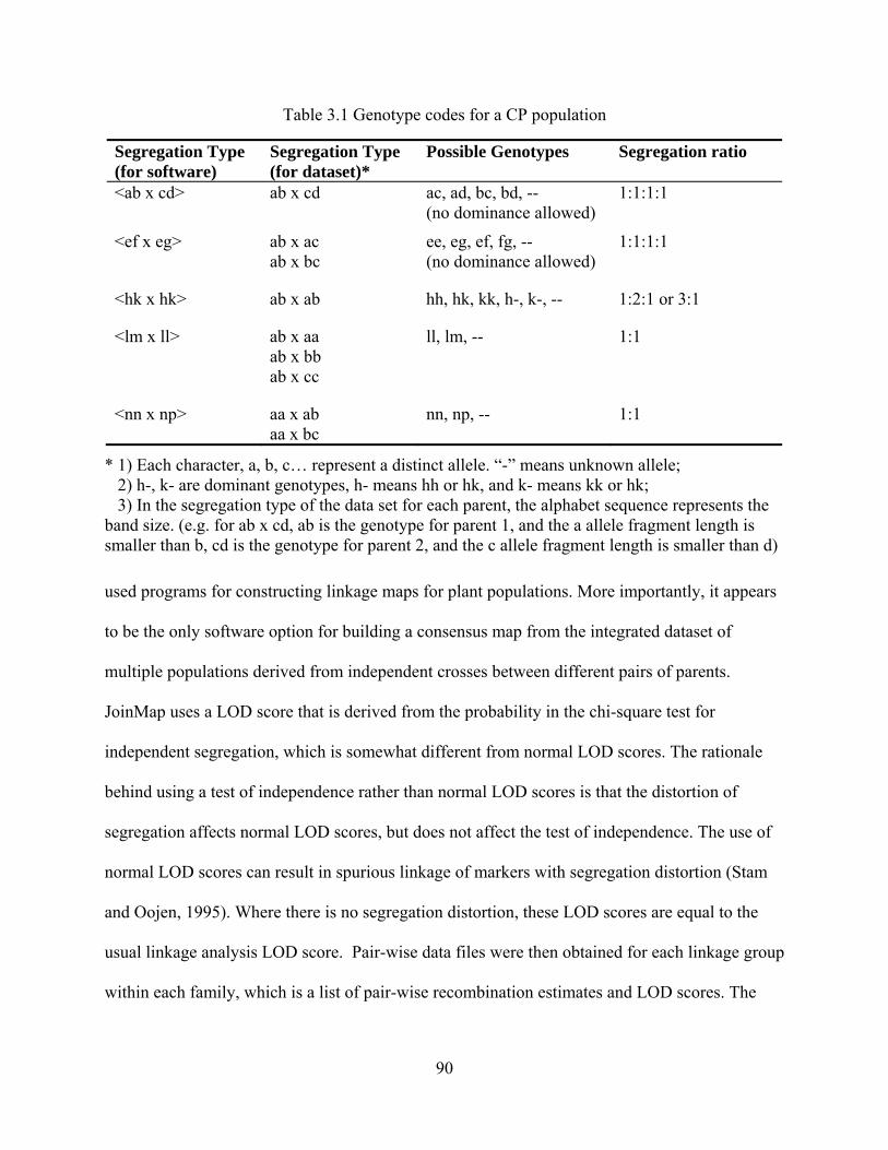
90
Table 3.1 Genotype codes for a CP population
Segregation Type (for software)
Segregation Type (for dataset)*
Possible Genotypes Segregation ratio
<ab x cd> ab x cd ac, ad, bc, bd, -- (no dominance allowed)
1:1:1:1
<ef x eg> ab x ac ab x bc
ee, eg, ef, fg, -- (no dominance allowed)
1:1:1:1
<hk x hk> ab x ab hh, hk, kk, h-, k-, -- 1:2:1 or 3:1
<lm x ll> ab x aa ab x bb ab x cc
ll, lm, -- 1:1
<nn x np> aa x ab aa x bc
nn, np, -- 1:1
* 1) Each character, a, b, c… represent a distinct allele. “-” means unknown allele; 2) h-, k- are dominant genotypes, h- means hh or hk, and k- means kk or hk; 3) In the segregation type of the data set for each parent, the alphabet sequence represents the band size. (e.g. for ab x cd, ab is the genotype for parent 1, and the a allele fragment length is smaller than b, cd is the genotype for parent 2, and the c allele fragment length is smaller than d)
used programs for constructing linkage maps for plant populations. More importantly, it appears
to be the only software option for building a consensus map from the integrated dataset of
multiple populations derived from independent crosses between different pairs of parents.
JoinMap uses a LOD score that is derived from the probability in the chi-square test for
independent segregation, which is somewhat different from normal LOD scores. The rationale
behind using a test of independence rather than normal LOD scores is that the distortion of
segregation affects normal LOD scores, but does not affect the test of independence. The use of
normal LOD scores can result in spurious linkage of markers with segregation distortion (Stam
and Oojen, 1995). Where there is no segregation distortion, these LOD scores are equal to the
usual linkage analysis LOD score. Pair-wise data files were then obtained for each linkage group
within each family, which is a list of pair-wise recombination estimates and LOD scores. The

91
other linkage analyses parameters, such as weak linkages, strong linkages, and suspect linkages,
were to follow the default parameters of the software.
Segregation of the loci was first tested for deviation from expected Mendelian
segregation by chi-square analysis. Those markers that showed highly significant segregation
distortion (P<0.005) were excluded from further map construction. Linkage groupings were
made using a logarithm of odds ratio (LOD) threshold of 4 and maximum recombination
frequency θ=0.45. Map distances in cM were calculated using both Haldane’s and Kosambi’s
mapping function. The map distance calculated with Haldane’s mapping function was labeled as
cM (H) and the map distance calculated with Kosambi’s mapping function was labeled as cM (K)
as described by Nelson et al. (1994).
Locus ordering and linkage map extension with JoinMap involved three cycles of data
shuffling to find the best fitting linear order of markers. The best-fitting order determined by the
change or ‘jump’ in goodness-of-fit of the map after a marker was inserted and controlled by the
‘jump’ parameter. During the first cycle, only the markers that caused a ‘jump’ or increase in the
chi-square value smaller than the specified threshold (i.e. LOD=4.0) were positioned. Markers
that caused a ‘jump’ greater than 4.0 were not discarded, but were temporarily kept aside
because the change in the chi-square value not only depended on the marker itself, but also on
the markers already on the map (Stam and Ooijen, 1995). During the second round of map
construction, JoinMap attempted to position these markers using the same fitting criterion as in
the first round. Thus, the markers ordered during the first and second round of map construction
considered as “framework” markers since they were placed with a high degree of stringency. In
the third round, all previously removed loci were given a final attempt to be added to the map by
ignoring the requirements of maximum allowed reduction in goodness-of-fit and no negative
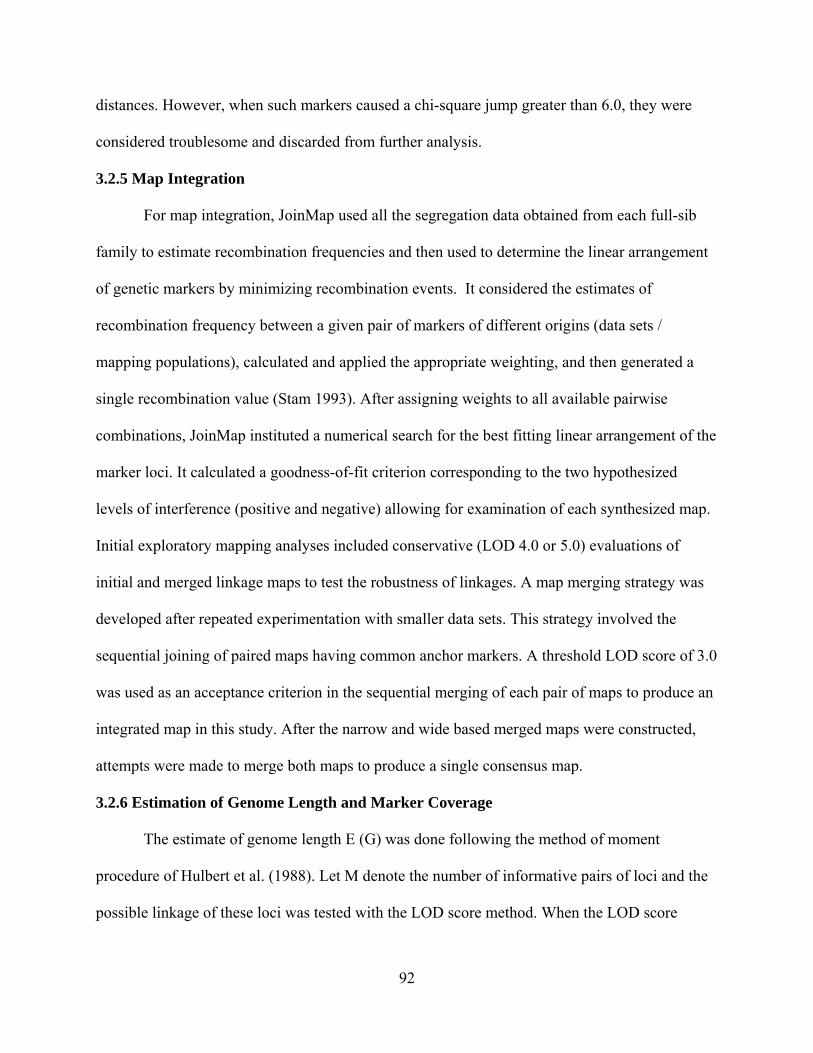
92
distances. However, when such markers caused a chi-square jump greater than 6.0, they were
considered troublesome and discarded from further analysis.
3.2.5 Map Integration
For map integration, JoinMap used all the segregation data obtained from each full-sib
family to estimate recombination frequencies and then used to determine the linear arrangement
of genetic markers by minimizing recombination events. It considered the estimates of
recombination frequency between a given pair of markers of different origins (data sets /
mapping populations), calculated and applied the appropriate weighting, and then generated a
single recombination value (Stam 1993). After assigning weights to all available pairwise
combinations, JoinMap instituted a numerical search for the best fitting linear arrangement of the
marker loci. It calculated a goodness-of-fit criterion corresponding to the two hypothesized
levels of interference (positive and negative) allowing for examination of each synthesized map.
Initial exploratory mapping analyses included conservative (LOD 4.0 or 5.0) evaluations of
initial and merged linkage maps to test the robustness of linkages. A map merging strategy was
developed after repeated experimentation with smaller data sets. This strategy involved the
sequential joining of paired maps having common anchor markers. A threshold LOD score of 3.0
was used as an acceptance criterion in the sequential merging of each pair of maps to produce an
integrated map in this study. After the narrow and wide based merged maps were constructed,
attempts were made to merge both maps to produce a single consensus map.
3.2.6 Estimation of Genome Length and Marker Coverage
The estimate of genome length E (G) was done following the method of moment
procedure of Hulbert et al. (1988). Let M denote the number of informative pairs of loci and the
possible linkage of these loci was tested with the LOD score method. When the LOD score

93
exceeded a certain threshold Z, the loci were assumed to be linked. Let K denote the number of
such pairs and the ratio K/M was then the probability that a pair of loci chosen at random would
be declared linked. This probability can also be expressed as a function of G, the genome length,
and X, the map distance between two loci for which a LOD score was expected. It was equal to
2X/G. The estimate genome length E (G) was then expressed as:
E(G)= 2MX⁄
where M=m (m-1)/2 and n was the number of framework markers. The value of K was obtained
from the linkages tab from JoinMap results panel.
The confidence interval for G, Iα (G) was calculated from the equation
Iα G E G 1 nαK‐12 ‐1
where nα=1.96 for an α of 5% (Gerber and Rodolphe 1994; Echt et al., 1997). Only the
framework markers were used to avoid an overestimate of genome coverage (Grattapaglia and
Sederoff, 1994).
The observed genome map Go was calculated by the formula of Nelson et al. (1994),
which takes into account all markers, linked and unlinked:
Go=GF+ X (L-R)
where GF is the total length of framework map, X is the observed maximum distance between
two framework markers, L is the total number of linkage groups, pairs and unlinked loci, and R
is the haploid number of chromosomes (Nelson et al., 1994; Echt et al., 1997).
The expected genome coverage, E (Cn) % (Bishop et al., 1983), was calculated from
pairwise segregation data for marker pairs above a threshold LOD of 3.0.
E Cn =1-P1,n
where

94
P1,n=2Rn+1
1-X2G
n+1
- 1-XG
n+1
+ 1-RXG
1-XG
n
where R is the number of chromosome (R=12 for longleaf pine), X is the maximum distance
under Z, and G is the expected genome length.
3.3 Results
3.3.1 Allele Frequencies and Parentage Analyses
There are 123 out of 135 polymorphic SSR markers showed polymorphisms in the
Derr488 half-sib family. All these polymorphic markers were tested for allele number (k),
observed heterozygosity (Hobs), expected heterozygosity (HExp), polymorphic information
content (PIC), null allele frequence (FNull), and the deviation of genotypic frequencies from
Hardy-Weinberg equilibrium. The mean and standard deviation of these parameters are listed in
Table 3.2. The individual marker estimation for all polymorphic markers is listed in appendix B.
Table 3.2 Summary for allele frequencies estimation obtained from CERVUS
Variable Mean Std Dev Minimum Maximum
k 3.8 1.94 2 9
HObs 0.62 0.17 0.37 1
HExp 0.53 0.15 0.3 0.82
PIC 0.47 0.16 0.25 0.8
FNull -0.08 0.08 -0.26 0.17
The observed heterozygosity is the number of heterozygotes divided by the total number
of individuals typed. The expected heterozygosity is calculated by using an unbiased formula
from allele frequencies assuming Hardy-Weinberg equilibrium (equation 8.4, Nei 1987).
Expected heterozygosity is a very useful measure of informativeness of a locus. The expected
heterozygosity generally differs from the observed heterozygosity because it is a prediction
based on the known allele frequency from a sample of individuals. The observed heterozygosity

95
for the polymorphic markers ranged from 0.37 to 1.00 with the mean value 0.62, and the
expected heterozygosity ranged from 0.30 to 0.82 with the mean value of 0.53. For all the
markers typed, PtTX_4093, SsrPt_ctg, and ript0079 showed the highest observed
heterozygosity (0.99, 1, and 1 respectively), while ript1027, ript0079, and PtTX_3116 showed
the highest expected heterozygosity (0.82). Sifg1008, sifg1069, and PtTX_2094 had the
smallest observed and expected heterozygosity value (Appendix B).
Polymorphic information content (PIC) is a measure of informativeness related to
expected heterozygosity and is likewise calculated from allele frequencies (Botstein et al., 1980;
Hearne et al., 1992). It is commonly used in linkage mapping, and preferential selection of
markers with high PIC values will increase the marker polymorphism rate in a cross in which
allele sizes for the parental strains are not known (Patterson, et al., 1995). The PIC value ranged
from 0.25 to 0.82 and with the mean value of 0.47. The three markers, sifg1008, sifg1069, and
PtTX_2094, which had the smallest expected heterozygosity, had the smallest PIC. The three
highest expected heterozygosity markers also had the highest PIC value (0.25, 0.27, and 0.28).
PIC values are usually smaller than corresponding expected heterozygosity and a large number
of alleles per locus usually corresponding high value of PIC and expected heterozygosity
(Figure 3.1). But this was not always true, e.g., ript0791 has 4 alleles per locus, however, its
expected heterozygosity and PIC values was smaller than all those with 3 alleles markers and
the majority of those with 2 alleles markers.
A null allele is any allele that cannot be detected by the assay used to genotype
individuals at a particular locus. A locus with a large positive estimate of null allele frequency
indicates an excess of homozygotes, but does not necessarily imply that a null allele is present.
However, the loci with large null allele frequencies were usually suspected for null alleles. Thirty
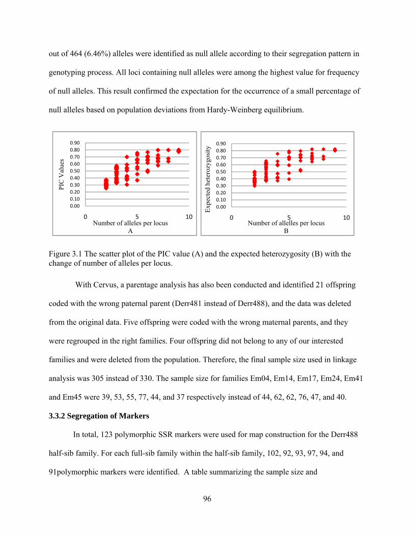
96
out of 464 (6.46%) alleles were identified as null allele according to their segregation pattern in
genotyping process. All loci containing null alleles were among the highest value for frequency
of null alleles. This result confirmed the expectation for the occurrence of a small percentage of
null alleles based on population deviations from Hardy-Weinberg equilibrium.
Figure 3.1 The scatter plot of the PIC value (A) and the expected heterozygosity (B) with the change of number of alleles per locus.
With Cervus, a parentage analysis has also been conducted and identified 21 offspring
coded with the wrong paternal parent (Derr481 instead of Derr488), and the data was deleted
from the original data. Five offspring were coded with the wrong maternal parents, and they
were regrouped in the right families. Four offspring did not belong to any of our interested
families and were deleted from the population. Therefore, the final sample size used in linkage
analysis was 305 instead of 330. The sample size for families Em04, Em14, Em17, Em24, Em41
and Em45 were 39, 53, 55, 77, 44, and 37 respectively instead of 44, 62, 62, 76, 47, and 40.
3.3.2 Segregation of Markers
In total, 123 polymorphic SSR markers were used for map construction for the Derr488
half-sib family. For each full-sib family within the half-sib family, 102, 92, 93, 97, 94, and
91polymorphic markers were identified. A table summarizing the sample size and
0.000.100.200.300.400.500.600.700.800.90
0 5 10
PIC
Val
ues
Number of alleles per locusA
0.000.100.200.300.400.500.600.700.800.90
0 5 10
Expe
cted
hete
rozy
gosi
ty
Number of allelles per locusB
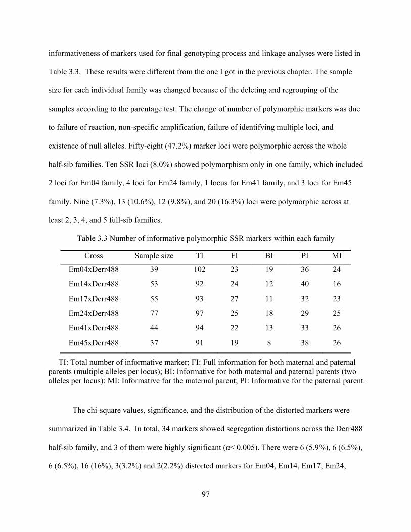
97
informativeness of markers used for final genotyping process and linkage analyses were listed in
Table 3.3. These results were different from the one I got in the previous chapter. The sample
size for each individual family was changed because of the deleting and regrouping of the
samples according to the parentage test. The change of number of polymorphic markers was due
to failure of reaction, non-specific amplification, failure of identifying multiple loci, and
existence of null alleles. Fifty-eight (47.2%) marker loci were polymorphic across the whole
half-sib families. Ten SSR loci (8.0%) showed polymorphism only in one family, which included
2 loci for Em04 family, 4 loci for Em24 family, 1 locus for Em41 family, and 3 loci for Em45
family. Nine (7.3%), 13 (10.6%), 12 (9.8%), and 20 (16.3%) loci were polymorphic across at
least 2, 3, 4, and 5 full-sib families.
Table 3.3 Number of informative polymorphic SSR markers within each family
Cross Sample size TI FI BI PI MI
Em04xDerr488 39 102 23 19 36 24
Em14xDerr488 53 92 24 12 40 16
Em17xDerr488 55 93 27 11 32 23
Em24xDerr488 77 97 25 18 29 25
Em41xDerr488 44 94 22 13 33 26
Em45xDerr488 37 91 19 8 38 26
TI: Total number of informative marker; FI: Full information for both maternal and paternal parents (multiple alleles per locus); BI: Informative for both maternal and paternal parents (two alleles per locus); MI: Informative for the maternal parent; PI: Informative for the paternal parent.
The chi-square values, significance, and the distribution of the distorted markers were
summarized in Table 3.4. In total, 34 markers showed segregation distortions across the Derr488
half-sib family, and 3 of them were highly significant (α< 0.005). There were 6 (5.9%), 6 (6.5%),
6 (6.5%), 16 (16%), 3(3.2%) and 2(2.2%) distorted markers for Em04, Em14, Em17, Em24,
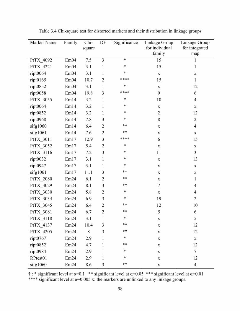
98
Table 3.4 Chi-square test for distorted markers and their distribution in linkage groups Marker Name Family Chi-
square DF †Significance Linkage Group
for individual family
Linkage Group for integrated
map PtTX_4092 Em04 7.5 3 * 15 1 PtTX_4221 Em04 3.1 1 * 15 1 ript0064 Em04 3.1 1 * x x ript0165 Em04 10.7 2 **** 15 1 ript0852 Em04 3.1 1 * x 12 ript9058 Em04 19.8 3 **** 9 6 PtTX_3055 Em14 3.2 1 * 10 4 ript0064 Em14 3.2 1 * x x ript0852 Em14 3.2 1 * 2 12 ript0968 Em14 7.8 3 * 8 2 sifg1060 Em14 6.4 2 ** x 4 sifg1061 Em14 7.6 2 ** x x PtTX_3011 Em17 12.9 3 **** 6 15 PtTX_3052 Em17 5.4 2 * x x PtTX_3116 Em17 7.2 3 * 11 3 ript0032 Em17 3.1 1 * x 13 ript0947 Em17 3.1 1 * x x sifg1061 Em17 11.1 3 ** x x PtTX_2080 Em24 6.1 2 ** x 1 PtTX_3029 Em24 8.1 3 ** 7 4 PtTX_3030 Em24 5.8 2 * x 4 PtTX_3034 Em24 6.9 3 * 19 2 PtTX_3045 Em24 6.4 2 ** 12 10 PtTX_3081 Em24 6.7 2 ** 5 6 PtTX_3118 Em24 3.1 1 * x 5 PtTX_4137 Em24 10.4 3 ** x 12 PtTX_4205 Em24 8 3 ** x 12 ript0767 Em24 2.9 1 * x x ript0852 Em24 4.7 1 ** x 12 ript0984 Em24 2.9 1 * x 7 RPtest01 Em24 2.9 1 * x 12 sifg1060 Em24 8.6 3 ** x 4
† : * significant level at α=0.1 ** significant level at α=0.05 *** significant level at α=0.01 **** significant level at α=0.005 x: the markers are unlinked to any linkage groups.

99
Table 3.4 Continued
Marker Name Family Chi-square
DF †Significance Linkage Group for individual
family
Linkage Group for integrated
map sifg1064 Em24 9.1 2 ** 19 2 SsrPt_ctg4698 Em24 9.5 3 ** x 5 PtTX_2094 Em41 3.3 1 * x 2 PtTX_4030 Em41 8.2 3 ** x 7 ript0065 Em41 5.8 1 ** 11 5 PtTX_3049 Em45 8.3 3 ** x 4 sifg1055 Em45 6.6 3 * x 4
Em41, and Em45 full-sib families, respectively. Four markers distorted across at least two
families, (e.g. ript0064 for family Em04 and Em14; ript0852 for family Em04, Em14, and Em24;
sifg1060 for family E14 and family Em24; sifg1061 for family Em14 and Em17). The other
distorted markers were specific to each family. These distorted markers were discarded in the
first round of linkage analysis for framework markers.
The distorted markers were placed on the linkage map at the second run of the map
construction because the distribution of the distorted markers was important for genome structure
study. For each full-sib families, 2 of 6 (33%), 3 of 6 (50%), 4 of 6 (67%), 11 of 16 (69%), 2 of 3
(67%), and 2 of 2 (100%) distorted markers could not combined to any linkage groups, even
when under LOD threshold 2.0. The other distorted markers tended to scattered in 1 or 2 linkage
groups in each full-sib family. Seven distorted markers could not combine to any linkage group
for integrated maps, and the other distorted markers were distributed on 11 linkage groups.
Reasons for skewed segregation ratios of molecular markers are still not well understood,
but are generally believed to be related to genetic factors such as chromosome loss and structural
rearrangements (Williams et al., 1995; Kuang et al., 1999), genetic isolating mechanisms (Zamir
and Tadmor, 1986), and other non-biological factors, like sampling in finite mapping population

100
or scoring errors (Plomion et al., 1995). The null allele (6.46%) also had effects on the
segregation distortion. Eleven of 34 (32.4%) distorted markers contained null alleles.
3.3.3 Construction of Linkage Map for the Individual Family
The estimates of observed recombination distance, mean interval, and percentage of
framework markers for each individual family were summarized at Table 3.5. At the LOD
threshold for linkage of 4.0 and θ=0.40, 68.6%, 70.7%, 66.7%, 74.2%, 55.3%, and 56.0% of
polymorphic loci were mapped to 19, 19, 17, 19, 18, and 17 linkage groups for each full-sib
family. Note the percentage of linked markers was small for each mapping population. This may
caused by the small sample size and number of polymorphic markers used for each family. The
family Em24 had the largest family size (e.g.77), and thus the largest percentage of linked
markers (74.2%). However, the number of sample size and number of linked markers was not as
simple as a linear relationship. The number of polymorphic markers and their linkage
relationships also played a very important role. The results also showed that the linkage maps for
individual families were not complete because the pines have 12 pairs of chromosomes, while
the linkage groups in each individual family were more than that. Family 24 had the largest
genetic length and percentage of framework markers. Family Em14 had the largest mean interval
(e.g. 17.6 cM (H) and 12.2 cM (K)). The results in Table 3.3 and Table 3.5 suggested that
increasing the sample size and number of polymorphic markers would be useful for increasing
genetic length and decreasing mean interval.
The comparison of different linkage groups for each mapping population is shown in
Figure 3.2. For each picture in Figure 3.2, the linkage groups came from different families with
common markers were put together for comparison their differences in marker order and
distances. Only the linkage groups with common markers across 6 full-sib families were shown
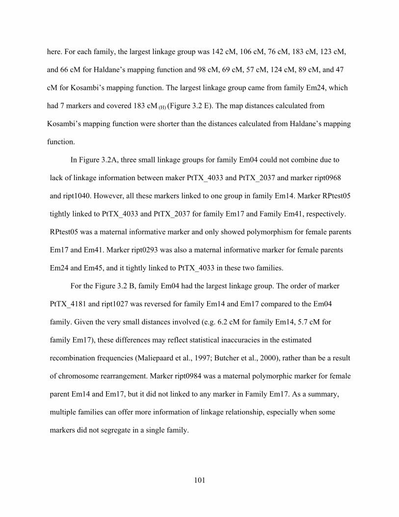
101
here. For each family, the largest linkage group was 142 cM, 106 cM, 76 cM, 183 cM, 123 cM,
and 66 cM for Haldane’s mapping function and 98 cM, 69 cM, 57 cM, 124 cM, 89 cM, and 47
cM for Kosambi’s mapping function. The largest linkage group came from family Em24, which
had 7 markers and covered 183 cM (H) (Figure 3.2 E). The map distances calculated from
Kosambi’s mapping function were shorter than the distances calculated from Haldane’s mapping
function.
In Figure 3.2A, three small linkage groups for family Em04 could not combine due to
lack of linkage information between maker PtTX_4033 and PtTX_2037 and marker ript0968
and ript1040. However, all these markers linked to one group in family Em14. Marker RPtest05
tightly linked to PtTX_4033 and PtTX_2037 for family Em17 and Family Em41, respectively.
RPtest05 was a maternal informative marker and only showed polymorphism for female parents
Em17 and Em41. Marker ript0293 was also a maternal informative marker for female parents
Em24 and Em45, and it tightly linked to PtTX_4033 in these two families.
For the Figure 3.2 B, family Em04 had the largest linkage group. The order of marker
PtTX_4181 and ript1027 was reversed for family Em14 and Em17 compared to the Em04
family. Given the very small distances involved (e.g. 6.2 cM for family Em14, 5.7 cM for
family Em17), these differences may reflect statistical inaccuracies in the estimated
recombination frequencies (Maliepaard et al., 1997; Butcher et al., 2000), rather than be a result
of chromosome rearrangement. Marker ript0984 was a maternal polymorphic marker for female
parent Em14 and Em17, but it did not linked to any marker in Family Em17. As a summary,
multiple families can offer more information of linkage relationship, especially when some
markers did not segregate in a single family.

102
Table 3.5 Comparison of linkage groups, marker numbers, genetic length and mean interval between markers in the SSR-based linkage map for each full-sib family
Family No. L.G. Total No.
Markers No. linked Markers
Genetic Length(H)
Mean Interval(H)
Genetic Length(K)
Mean Interval(k)
Percent of framework
Em04 19 102 70 976 13.9 629 9.0 63.8
Em14 19 92 65 1146 17.6 796 12.2 64.2
Em17 17 93 62 658 10.6 528 8.5 62.3
Em24 19 97 72 1190 16.5 743 10.3 67.0
Em41 18 94 52 598 11.5 411 7.9 54.3
Em45 18 91 51 575 11.3 348 6.8 56.0
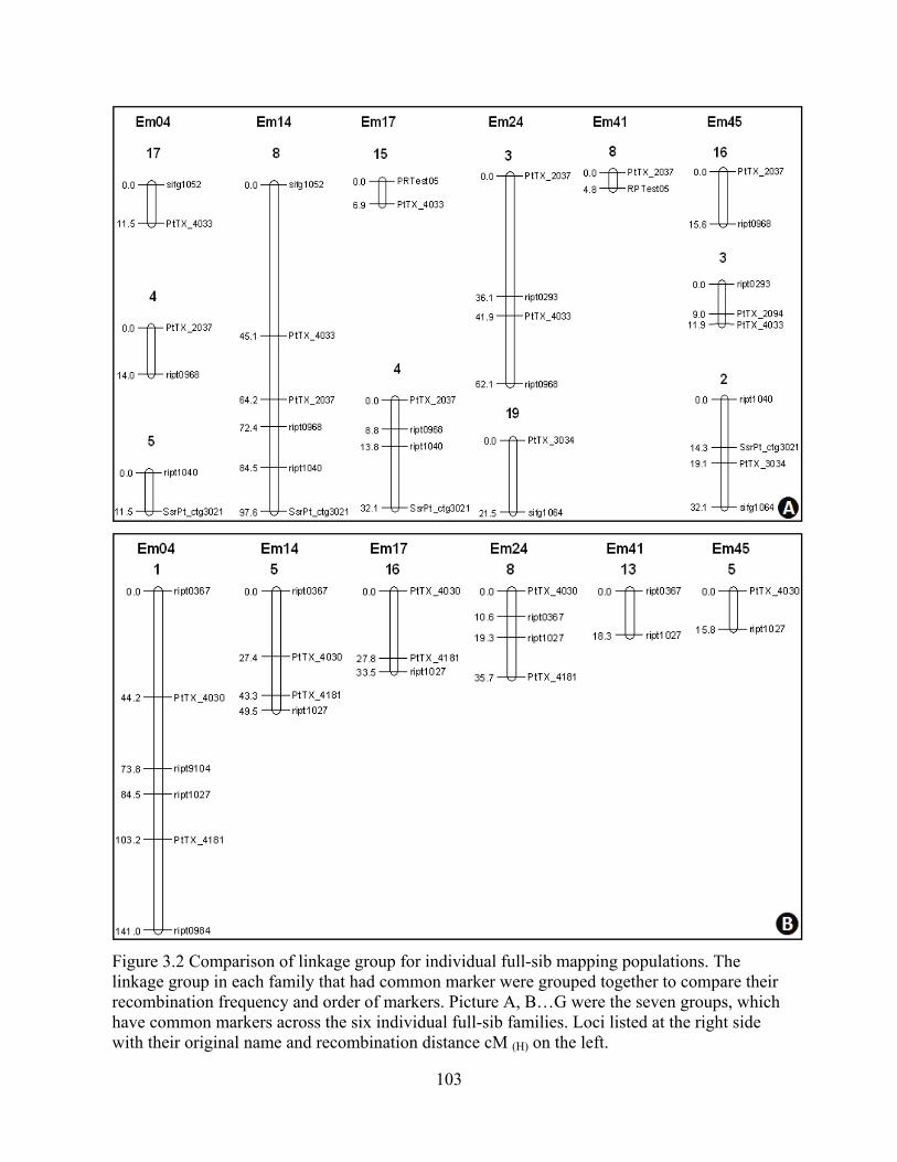
103
Figure 3.2 Comparison of linkage group for individual full-sib mapping populations. The linkage group in each family that had common marker were grouped together to compare their recombination frequency and order of markers. Picture A, B…G were the seven groups, which have common markers across the six individual full-sib families. Loci listed at the right side with their original name and recombination distance cM (H) on the left.

104
Figure 3.2 Continued

105
Figure 3.2 Continued

106
Figure 3.2 Continued
3.3.4 Integrated Maps from Six Full-Sib Families
The family Em24 was treated as the basic map because of its largest sample size and
number of linked markers. The other families were integrated one by one according to the order
of their sample size and number of linked markers. There were 110 markers mapped to 16
linkage groups, and three of the linkage groups had only 2 markers. The linkage groups 15 and
16 both contain marker PtTX_3011, however, there was not enough linkage information to group
them into one linkage group. The linkage relationship between PtTX_3011 and PtTX_3019 was
observed in 5 families, while the linkage relationship of PtTX_3011 and SsrPt_ctg3754 was only
observed in Family Em45. The marker SsrPt_ctg3754 was a maternal polymorphic marker and
only showed polymorphism for Family Em24 and Em45; it did not combined to any linkage
group in Family Em24. The 16 linkage groups covered 1290 cM (H) with a mean interval of 11.4
cM (H). The largest linkage group contained 25 markers and covered 199 cM (H). The largest mean
interval was 27.5 cM (H) for linkage group 8. The detailed information was summarized in Table
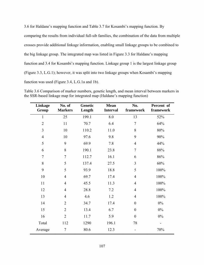
107
3.6 for Haldane’s mapping function and Table 3.7 for Kosambi’s mapping function. By
comparing the results from individual full-sib families, the combination of the data from multiple
crosses provide additional linkage information, enabling small linkage groups to be combined to
the big linkage group. The integrated map was listed in Figure 3.3 for Haldane’s mapping
function and 3.4 for Kosambi’s mapping function. Linkage group 1 is the largest linkage group
(Figure 3.3, L.G.1); however, it was split into two linkage groups when Kosambi’s mapping
function was used (Figure 3.4, L.G.1a and 1b).
Table 3.6 Comparison of marker numbers, genetic length, and mean interval between markers in the SSR-based linkage map for integrated map (Haldane’s mapping function)
Linkage Group
No. of Markers
Genetic Length
Mean Interval
No. framework
Percent of framework
1 25 199.1 8.0 13 52%
2 11 70.7 6.4 7 64%
3 10 110.2 11.0 8 80%
4 10 97.6 9.8 9 90%
5 9 69.9 7.8 4 44%
6 8 190.1 23.8 7 88%
7 7 112.7 16.1 6 86%
8 5 137.4 27.5 3 60%
9 5 93.9 18.8 5 100%
10 4 69.7 17.4 4 100%
11 4 45.5 11.3 4 100%
12 4 28.8 7.2 4 100%
13 4 4.6 1.2 4 100%
14 2 34.7 17.4 0 0%
15 2 13.4 6.7 0 0%
16 2 11.7 5.9 0 0%
Total 112 1290 196.1 78 -
Average 7 80.6 12.3 - 70%

108
Table 3.7 Comparison of marker numbers, genetic length, and mean interval between markers in the SSR-based linkage map for integrated map (Kosambi’s mapping function)
Linkage Group
No. of Markers
Genetic Length
Mean Interval
No. framework
Percent of framework
1a 18 91.8 5.1 12 67%
1b 7 28.7 4.1 6 86%
2 10 48.0 4.8 9 90%
3 10 72.5 7.3 4 40%
4 10 80.0 8.0 9 90%
5 9 52.8 5.9 6 67%
6 8 94.2 11.8 6 75%
7 7 94.5 13.5 6 86%
8 5 81.8 16.4 5 100%
9 5 82.4 16.5 5 100%
10 4 53.9 13.5 4 100%
11 4 37.3 9.3 4 100%
12 4 21.4 5.4 4 100%
13 4 13.2 3.3 4 100%
14 2 27.5 13.8 0 0%
15 2 12.0 6.0 0 0%
16 2 10.6 5.3 0 0%
Total 111 902.6 149.7 84 -
Average 7 56.4 9.4 - 76%
There were 8 linkage groups that had distances between adjacent markers greater than 25
cM (H), namely ript0647 and ript0159 on group 1 (30.8cM), PtTX_2146 and RPtest09 on Group
3 (44.8 cM), ript0690 and ript9058 (54.5 cM), ript0001 and SsrPt_ctg7444 (58.1 cM), and
SsrPt_ctg7444 and sifg1069 (40.6 cM) on linkage group 6, ript0211 and PtTX_4181

109
Figure 3.3 An integrated SSR-based genetic map constructed by 112 polymorphic SSR markers with Haldane’s mapping function. Three hundred and five samples come from a half-sib family. Loci listed at the right side and cumulative recombination distance (cM (H)) on the left. The markers with * at the right side are the framework markers. A was for Haldane’s mapping function and B was for the Kosambi’s mapping function.
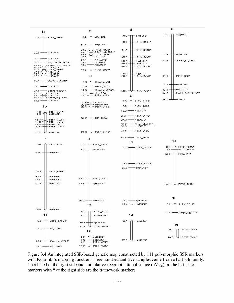
110
Figure 3.4 An integrated SSR-based genetic map constructed by 111 polymorphic SSR markers with Kosambi’s mapping function.Three hundred and five samples come from a half-sib family. Loci listed at the right side and cumulative recombination distance (cM (k)) on the left. The markers with * at the right side are the framework markers.
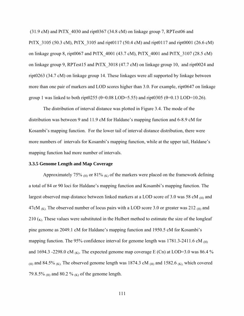
111
(31.9 cM) and PtTX_4030 and ript0367 (34.8 cM) on linkage group 7, RPTest06 and
PtTX_3105 (50.3 cM), PtTX_3105 and ript0117 (50.4 cM) and ript0117 and ript0001 (26.6 cM)
on linkage group 8, ript0067 and PtTX_4001 (43.7 cM), PtTX_4001 and PtTX_3107 (28.5 cM)
on linkage group 9, RPTest15 and PtTX_3018 (47.7 cM) on linkage group 10, and ript0024 and
ript0263 (34.7 cM) on linkage group 14. These linkages were all supported by linkage between
more than one pair of markers and LOD scores higher than 3.0. For example, ript0647 on linkage
group 1 was linked to both ript0255 (θ=0.08 LOD=5.55) and ript0305 (θ=0.13 LOD=10.26).
The distribution of interval distance was plotted in Figure 3.4. The mode of the
distribution was between 9 and 11.9 cM for Haldane’s mapping function and 6-8.9 cM for
Kosambi’s mapping function. For the lower tail of interval distance distribution, there were
more numbers of intervals for Kosambi’s mapping function, while at the upper tail, Haldane’s
mapping function had more number of intervals.
3.3.5 Genome Length and Map Coverage
Approximately 75% (H) or 81% (K) of the markers were placed on the framework defining
a total of 84 or 90 loci for Haldane’s mapping function and Kosambi’s mapping function. The
largest observed map distance between linked markers at a LOD score of 3.0 was 58 cM (H) and
47cM (K). The observed number of locus pairs with a LOD score 3.0 or greater was 212 (H) and
210 (K). These values were substituted in the Hulbert method to estimate the size of the longleaf
pine genome as 2049.1 cM for Haldane’s mapping function and 1950.5 cM for Kosambi’s
mapping function. The 95% confidence interval for genome length was 1781.3-2411.6 cM (H)
and 1694.3 -2298.0 cM (K). The expected genome map coverage E (Cn) at LOD=3.0 was 86.4 %
(H) and 84.5% (K). The observed genome length was 1874.3 cM (H) and 1582.6 (K), which covered
79.8.5% (H) and 80.2 % (K) of the genome length.

Figure 3.The X-axintervals
3.4 Discu
3.4.1 Het
F
the locus
degree of
Quantitat
one is he
informati
study, the
heterozyg
heterozyg
more alle
.5 The distribxis is the intein the corre
ussion
terozygosity
or a mating
s. Therefore,
f polymorph
tively, the de
eterozygosity
ion content (
e PIC value
gosity was s
gosity and P
eles in one lo
0
5
10
15
20
25
Num
ber o
f Intervals
bution of interval distancsponding int
y and Polym
to be inform
the usefulne
hism (i.e., its
egree of poly
y (Nei and R
(PIC) value
was smaller
smaller than
PIC value wa
ocus usually
terval distance (cM) of twtervals.
morphic Info
mative, at lea
ess of a mark
alleles and
ymorphism o
Roychoudhur
(Botstein et
r than the exp
the observed
as not direct
y had high he
Interval
112
ce between awo adjacent
formation C
ast one of the
ker in a mod
their frequen
of markers i
ry 1974), and
al., 1980). F
pected heter
d heterozygo
but was very
eterozygosity
Distance (cM)
adjacent marmarkers. Th
Content
e two parents
del-based lin
ncies) (Guo
s measured b
d another on
For all the m
rozygosity, a
osity. The re
y closely rel
y and PIC va
rkers for thehe Y-axis is t
s must be he
nkage analys
and Elston,
by two distin
ne is the poly
markers estim
and the expec
elationship b
lated. The m
alue, but the
e integrated mthe number o
eterozygous
is depends o
1999).
nct quantitie
ymorphism
mated in this
cted
etween
markers that h
se results wa
Haldane
Kosambi
map. of
for
on its
es:
had
as

113
not absolute, i.e. marker ript0791 had 4 alleles, but the heterozygosity and PIC value was smaller
than all the 3-allele markers and majority of 2-allele markers. The estimate of mean expected
heterozygosity (0.53) was close to the results of Echt et al.(1996) estimation in eastern white
pine (0.515), but smaller than the estimation of 0.59 in Pinus.halepensis and P.brutia (Keys, et
al., 2000) and 0.85 for P. sylbestris (Soranze et al., 1998). The heterozygosity and PIC value
may be related to the length of the SSR marker sequence (Slavov et al., 2004) and also related to
the population studied.
3.4.2 Segregation Distortion
There was 5.9%, 6.5%, 6.5%, 16%, 3.2%, and 2.2% markers showed segregation
distortion in each individual full-sib family. Segregation distortion of markers in forest trees had
been a common problem in forest genome studies (Lemes, et al., 2002; Ritter et al., 2002; Tani et
al., 2003; Yin, et al., 2004; Woolbright, et al., 2008; Gill et al., 2006). Segregation distortion may
occur due to biological reasons, e.g. chromosome loss (Kasha and Kao, 1970), genetic isolation
mechanisms (Zamir and Tadmor, 1986), presence of lethal genes and/or fragment complexes
(overlapping fragments consisting of identically sized fragments) (Nikaido et al, 1999; Hansen et
al, 1999), and the expression of genetic load via a lethal recessive allele(Bradshaw and Stettler,
1995). Distortion in segregation can influence map construction (Zhang, et al., 2002,
Woolbrightwith, et al, 2008) and QTL detection (Bradshaw et al., 1994; Cervera et al., 2001, Yin
et al., 2004). These studies also suggest that markers showing segregation distortion due to
linkage with genes under selection may have important ecological consequences, and should
therefore be included in mapping studies of natural populations. However, a study by Säll and
Nilsson (1994) proved that the effect of these sources of segregation distortion on recombination
estimates was relatively small, and bias to marker order was negligible (Lin and Ritland, 1996).

114
Therefore, caution must be exercised when making conclusions involving QTL linked to
distorted markers (Woolright et al., 2008).
Non-biological reasons, such as scoring errors (Devey et al., 1994; Xu et al., 1997) and
sampling errors (Plomion et al., 1995, Echt and Nelson, 1997), may also lead to segregation
distortion in mapping studies. The errors associated with the non-biological reason were assumed
to have serious effects on recombination values (Hallden et al., 1996; Säll and Nilsson 1994).
Genotyping error is a major concern when molecular markers are used for parentage analysis.
Minimizing the rate of mistyping and avoiding markers with high frequencies of null alleles may
be crucial for obtaining unbiased estimates of gene flow and pollen contamination (Slavov et al.,
2004). With microsatellite loci, a null allele most often occurs because of mutations in one or
both primer binding sites, sufficient to prevent effective amplification of the microsatellite allele
(Dakin & Avise 2004). This problem is particularly common when the microsatellite locus
cloned in one species is applied to a different species using the same primers. A null allele
cannot be distinguished on gel from a homozygote for the only DNA fragment, which can be
scored in the same plant, which usually leaded to scoring errors. Thirty out of 464 (6.46%)
alleles were identified as null alleles according to their segregation pattern in genotyping
processes, and these results were matched with the null allele frequency results in CERVUS
output. Among the 34 distorted markers, 11 (32.4%) of them contain null alleles. Given the facts
that most distorted markers (88.23%) were specific for individual families and scattered to 11
linkage groups, the distorted segregation in this study is considered to be mostly caused by non-
biological reasons.
Microsatellite markers containing multiple loci can simultaneously detect two or more
loci were attractive and useful for some applications (Fisher et al., 1998; Amarasinge and

115
Carlson 2002). However, it was very hard to differentiate different loci when the amplification
products had similar sizes (Figure 3.5), if this marker also contained null alleles, it was
impossible to avoid genotyping error. The multiple locus and null alleles were also the main
reasons I used less markers for the linkage study than I screened in the previous chapters. Single
locus SSR markers were usually preferred in genome mapping studies.
Figure 3.6 Multiple locus SSR markers (sifg1004). The 1st, 18th, 35th, and 52nd are standard molecular weight. The other lines are DNA samples for backcross population.
3.4.3 The Integrated Map
Although several moderately dense linkage maps have been previously constructed for
longleaf and slash pine using RAPD makers, this was the first time a linkage map for longleaf
pine and longleaf pine by slash pine hybrid was made exclusively from microsatellite DNA
markers. The expected advantages of a microsatellite based linkage map, in contrast to a RAPD
based linkage map, was stability and portability to other families and pedigrees.
There were some problems associated with construction linkage maps in single family in
this study: there were up to 19 linkage groups for each individual family, but the homologous
chromosome number for pine trees was 12; each family had several linkage groups containing
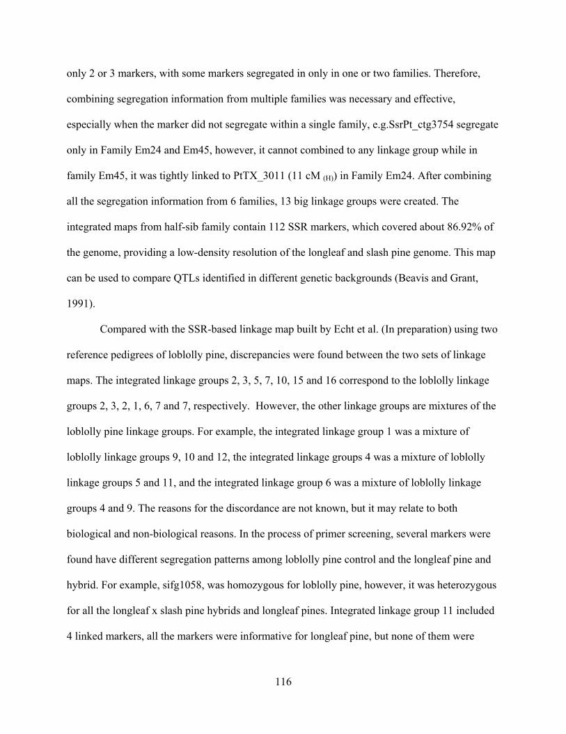
116
only 2 or 3 markers, with some markers segregated in only in one or two families. Therefore,
combining segregation information from multiple families was necessary and effective,
especially when the marker did not segregate within a single family, e.g.SsrPt_ctg3754 segregate
only in Family Em24 and Em45, however, it cannot combined to any linkage group while in
family Em45, it was tightly linked to PtTX_3011 (11 cM (H)) in Family Em24. After combining
all the segregation information from 6 families, 13 big linkage groups were created. The
integrated maps from half-sib family contain 112 SSR markers, which covered about 86.92% of
the genome, providing a low-density resolution of the longleaf and slash pine genome. This map
can be used to compare QTLs identified in different genetic backgrounds (Beavis and Grant,
1991).
Compared with the SSR-based linkage map built by Echt et al. (In preparation) using two
reference pedigrees of loblolly pine, discrepancies were found between the two sets of linkage
maps. The integrated linkage groups 2, 3, 5, 7, 10, 15 and 16 correspond to the loblolly linkage
groups 2, 3, 2, 1, 6, 7 and 7, respectively. However, the other linkage groups are mixtures of the
loblolly pine linkage groups. For example, the integrated linkage group 1 was a mixture of
loblolly linkage groups 9, 10 and 12, the integrated linkage groups 4 was a mixture of loblolly
linkage groups 5 and 11, and the integrated linkage group 6 was a mixture of loblolly linkage
groups 4 and 9. The reasons for the discordance are not known, but it may relate to both
biological and non-biological reasons. In the process of primer screening, several markers were
found have different segregation patterns among loblolly pine control and the longleaf pine and
hybrid. For example, sifg1058, was homozygous for loblolly pine, however, it was heterozygous
for all the longleaf x slash pine hybrids and longleaf pines. Integrated linkage group 11 included
4 linked markers, all the markers were informative for longleaf pine, but none of them were

117
identified as heterozygous for loblolly. This different segregation pattern may indicate some
major differences between longleaf pine and loblolly pine. The non-biological reasons also play
an important role on linkage analysis. Since the linkage relationship was analyzed based on the
individual full-sib family and followed by the integration from multiple families, the sample
sizes for each full-sib family were critical. Although there were 305 samples available for
linkage analyses, the sample size for each full-sib family was smaller compared with the loblolly
pedigrees, which reduce the power of linkage analyses. In the process of map integration, two
common markers were used in this study to join the linkage groups from different families. The
integrated linkage group 1 corresponds to the mixture of loblolly linkage groups of 9, 10, and 12.
However, with closer inspection of Figure 3.2 D (the source of integrated linkage group 1), it
can be found that if 3 common markers were used to join the linkage groups from the different
families, then 3 linkage groups would be created matching the results from the loblolly pine
linkage group. Therefore, caution must be taken in joining process to avoid false linkage
association.
According to Butcher (2000), the advantages of mapping multiple pedigrees include: a
large number of loci are mapped, gene order and map distances are estimated more accurately,
and alterations in these values, possibly due to chromosomal rearrangements affecting one of the
parents, are easily detected. The differences in recombination frequencies were observed in each
individual family and caused distortion of map distances between the relevant pairs of markers
on the integrated map. However, small discrepancies in marker order may caused by mapping
imprecision rather than real rearrangement (Lombard and Delourme, 2001).The large mean
marker interval, unlinked markers, 16 linkage groups, and the existence of 2 marker linkage

118
groups suggest that the integrated map was not complete and the linkage gaps remained to be
filled by adding more markers.
3.4.4 Genome Length and Map Coverage
The method of moment estimator of Hulbert et al (1988) is the most widely used function
for deducing genome length because it is easy to calculate from readily available genome
mapping data and statistics (Echt and Nelson, 1997). Chakravarti et al (1991) used a
modification of Hulbert’s method. For a given LOD score, Z, the pairs with the largest estimated
θ value was chosen from the pair of loci with LOD scores greater or equal than Z. In the
simulation experiment, Chakravarti et al. observed that the Hulbert method overestimated the
genetic distance. However, in this study, the Hulbert method always gave the smaller estimation
for both Kosambi and Haldane’s mapping function. Our results matched the conclusion obtained
by Gerber and Rodolphe (1994) in their study on maritime pine.
Genome length estimates in forest trees with different markers, pedigrees and computer
programs were obtained (Echt and Nelson, 1997; Barreneche et al., 1998; Devey et al., 1999;
Sewell et al., 1999; Lespinasse et al., 2000; Chagne et al., 2002, 2003; Wilcox et al., 2004;
Pelgas et al., 2006). Generally, a common assumption is that maps constructed with JoinMap are
shorter than those maps constructed with the multilocus-likelihood computer software, e.g.,
MapMaker and OutMap (Sewell et al., 1999; Butcher et al., 2002; Gosselin et al., 2002; Tani et
al., 2003). The multilocus-likelihood method used by MapMaker assumes an absence of
crossover interference, and map length was calculated as the sum of adjacent distances using
adjacent marker pairs only. The recombination frequencies were transferred to cM according to
the selected mapping function directly. However, JoinMap use all pairwise estimates for
estimating the map distance (Stam, 1993) and correctly produces shorter maps when an

119
interference exist even Kosambi’s mapping function was used in both programs (Stam, 1993).
The estimate of the genome length for longleaf pine and slash pine in this study was 2049 cM (H)
and 1959 cM (K) under LOD score 3.0 with JoinMap ver.3.0. This estimate was shorter than the
estimation of Echt and Nelson (1997) and Weng (1999), in which the expected genome length
was 2618 cM (H), 2000 cM (K) and 2400 cM (H) for longleaf pine. In the work of comparing three
pines, Pinus strobus, P. palustris and P. pinaster, Echt and Nelson (1997) estimated the average
theoretical length was close to 2000 cM (K).
The theoretical map distance was also found to be greater than the observed genome map
coverage for both mapping functions. The process of framework construction (Echt and Nelson,
1997) may cause the differences between expected and observed values, where the framework
only accounted for 70%. This result also suggests that additional informative markers would be
useful to join smaller groups and increase map coverage.
3.5 References
Arcade, A., Anselin, F., Faivre, R.P., Lesage, M.C., Laurans, F., Paques, L.E., Prat, D. 2000. Application of AFLP, RAPD and ISSR markers to genetic mapping of European larch and Japanese larch. Theor. Appl. Genet. 100: 299-307.
Beavis, W.D., Grant, D. 1991. A linkage map based on information from four F2 populations of maize (Zea mays L.). Theor. Appl. Genet. 82: 636-644.
Bishop, D.T, Cannings, C., Skolnick, M., Williamson, J.A. 1983. The number of polymorphic DNA clones required to map the human genome. In: Statistical Analysis of DNA Sequence Data. Edited by Weir, B.C. Dekker: New York. pp 181–200.
Botstein, D., White, R.L, Skolnick, M., Davies, R.W. 1980. Construction of a genetic linkage map in man using restriction fragment length polymorphisms. Am. J. Hum. Genet. 32: 314-331.
Bradshaw, H.D., Stettler, R.F. 1995. Molecular genetics of growth and development in Populus. IV. Mapping QTLs with large effect on growth, form and phenology traits in a forest tree. Genetics 139: 963-973.
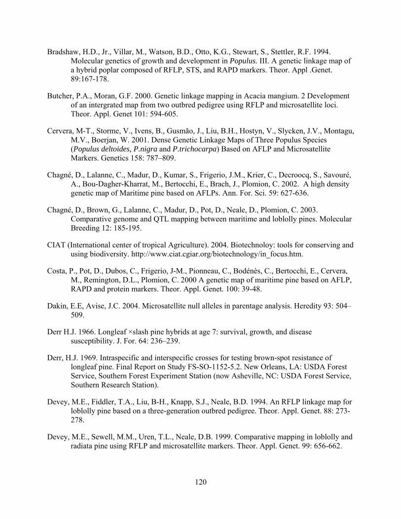
120
Bradshaw, H.D., Jr., Villar, M., Watson, B.D., Otto, K.G., Stewart, S., Stettler, R.F. 1994. Molecular genetics of growth and development in Populus. III. A genetic linkage map of a hybrid poplar composed of RFLP, STS, and RAPD markers. Theor. Appl .Genet. 89:167-178.
Butcher, P.A., Moran, G.F. 2000. Genetic linkage mapping in Acacia mangium. 2 Development of an intergrated map from two outbred pedigree using RFLP and microsatellite loci. Theor. Appl. Genet 101: 594-605.
Cervera, M-T., Storme, V., Ivens, B., Gusmão, J., Liu, B.H., Hostyn, V., Slycken, J.V., Montagu, M.V., Boerjan, W. 2001. Dense Genetic Linkage Maps of Three Populus Species (Populus deltoides, P.nigra and P.trichocarpa) Based on AFLP and Microsatellite Markers. Genetics 158: 787–809.
Chagné, D., Lalanne, C., Madur, D., Kumar, S., Frigerio, J.M., Krier, C., Decroocq, S., Savouré, A., Bou-Dagher-Kharrat, M., Bertocchi, E., Brach, J., Plomion, C. 2002. A high density genetic map of Maritime pine based on AFLPs. Ann. For. Sci. 59: 627-636.
Chagné, D., Brown, G., Lalanne, C., Madur, D., Pot, D., Neale, D., Plomion, C. 2003. Comparative genome and QTL mapping between maritime and loblolly pines. Molecular Breeding 12: 185-195.
CIAT (International center of tropical Agriculture). 2004. Biotechnoloy: tools for conserving and using biodiversity. http://www.ciat.cgiar.org/biotechnology/in_focus.htm.
Costa, P., Pot, D., Dubos, C., Frigerio, J-M., Pionneau, C., Bodénès, C., Bertocchi, E., Cervera, M., Remington, D.L., Plomion, C. 2000 A genetic map of maritime pine based on AFLP, RAPD and protein markers. Theor. Appl. Genet. 100: 39-48.
Dakin, E.E, Avise, J.C. 2004. Microsatellite null alleles in parentage analysis. Heredity 93: 504–509.
Derr H.J. 1966. Longleaf ×slash pine hybrids at age 7: survival, growth, and disease susceptibility. J. For. 64: 236–239.
Derr, H.J. 1969. Intraspecific and interspecific crosses for testing brown-spot resistance of longleaf pine. Final Report on Study FS-SO-1152-5.2. New Orleans, LA: USDA Forest Service, Southern Forest Experiment Station (now Asheville, NC: USDA Forest Service, Southern Research Station).
Devey, M.E., Fiddler, T.A., Liu, B-H., Knapp, S.J., Neale, B.D. 1994. An RFLP linkage map for loblolly pine based on a three-generation outbred pedigree. Theor. Appl. Genet. 88: 273-278.
Devey, M.E., Sewell, M.M., Uren, T.L., Neale, D.B. 1999. Comparative mapping in loblolly and radiata pine using RFLP and microsatellite markers. Theor. Appl. Genet. 99: 656-662.

121
Echt, C.S., May-Marquardt, P., Hseih, M., Zahorchak, R. 1996. Characterization of microsatellite markers in eastern white pine. Genome 39: 1102-1108.
Echt, C.S., Nelson, C.D. 1997. Linkage mapping and genome length in eastern white pine (Pinus strobus L.). Theor. Appl. Genet. 94: 1031-1037.
Echt, C.S., Saha, S., Krutovsky, K., Erpelding, J., Nelson, C.D. Microsatellite-based genetic map for loblolly pine ( In preparation).
Fisher, P.J., Richardson, T.E., Gardner, R.C. 1998. Characteristics of single- and multi-copy microsatellites from Pinus radiata. Theor. Appl. Genet. 96: 969-979.
Gentzbittel, L., Vear, F., Zhang, Y., Berville, A., Nicolas, P. 1995. Development of a consensus linkage RFLP map of cultivated sunflower (Helianthus annus L.). Theor. Appl. Genet. 90: 1079-1086.
Gerber, S. Rodolphf, F. 1994. An estimation of the genome length of maritime pine (Pinus pinaster Ait.). Theor. Appl. Genet. 88: 289-292.
Gill, G.P., Wilcox, P.L., Whittaker, D.J., Winz, R.A., Bickerstaff, P., Echt, C.E., Kent, J., Humphreys, M.O., Elborough, K.M., Gardner, R.C. 2006. A framework linkage map of perennial ryegrass based on SSR markers. Genome 49: 354-364.
Grattapaglia, D., Sederoff, R. 1994. Genetic linkage maps of Eucalyptus grandis and E. urophylla using a pseudo-testcross mapping strategy and RAPD markers. Genetics 137: 1121-1137.
Grattapaglia, D., Chaparro, J., Wilcox, P., McCord, S., Crane, B., Amerson, H., Werner, D., Liu, B.H., O’Malley, D., Whetten, R., Mckeand, S., Goldforb, B., Greenwoood, M., Kuhlman, G., Bridgewater, F., and Sederoff, R., 1993. Application of genetic markers to tree breeding, In: Proceedings of the 22nd Southern Forest Tree Improvement Conference, Atlanta, Georgia. 44: 452-463.
Guo, X., Elston, R.C. 1999. Linkage information content of polymorphic genetic markers. Hum.Hered. 49: 112-118.
Halldén, C., Nilsson, N.O., Rading, I.M., Säll, T. 1994. Evaluation of RFLP and RAPD markers in comparison of Brassica napus breeding lines. Theor. Appl. Genet. 88: 123-128.
Hansen, H., Kraft, T., Christiansson, M., Nilsson, N.O. 1999. Evaluation of AFLP in Beta. Theor. Appl. Genet. 98: 845–852.
Hauge, B., Hanley, S., Cartinhour, S. Cherry, J.M., Goodman, H.M. 1993. An integrated genetic/RFLP map of the Arabidopsis thaliana genome. Plant J. 3: 745-754.
Hayashi, E., Kondo, T., Terada, K., Kuramoto, N., Goto, Y., Okamura, M. 2001 Linkage map of Japanese black pine based on AFLP and RAPD markers including markers linked to

122
resistance against the pine needle gall midge. Theor. Appl. Genet. 102: 871-875.
Hulberts, H., Ilott, T.W., Lecg, E.J., Lincoln, S.E., Lander, E.S., Michelmore, R.W. 1988. Genetic analysis of the fungus, Bremia lactucae, using restriction fragment length polymorphisms. Genetics 120 947-958.
Kasha, K.J., Kao. K.N. 1970. High frequency haploid production in barley, (Hordeum vulgare L.). Nature (Lond.) 225: 874-876.
Keys, R.N., Autino, A., Edwards, K.J., Fady, B., Pichot, C., Vendramin, G.G. 2000. Characterization of nuclear microsatellites in Pinus halepensis Mill. and their inheritance in P. halepensis and P. brutia. Mol. Ecol. 9: 2157-2159.
Kianian, S.F. Quiros, C.F. 1992. Generation of a Brassica oleracea composite RFLP map: linkage arrangements among various populations and evolutionary implications. Theo. Appl. Genet. 84: 544-554.
Kuang, H., Richardson, T.E., Carson, S.D., Bongarten, B.C. 1999. Genetic analysis of inbreeding depression in plus tree 850.55 of Pinus radiata D. Don. II. Genetics of viability genes. Theor. Appl. Genet. 99: 140–146.
Kubisiak, T. L., Nelson, C.D., Nance, W.L., Stine, M. 1995. RAPD linkage mapping in a longleaf pine x slash pine F1 family. Theor. Appl. Genet. 90: 191-127.
Lemes, M.R., Brondani, R.R.V., Grattapagia, D. 2002. Multiplexed System of Microsatellite markers for genetic analysis of mahogany, Swietenia macrophylla King (Meliaceae), a threatened neotropical timber species. J. Hered. 93: 287-291.
Lin, J., Ritland, K. 1996. The effects of selective genotyping on estimates of proportion of recombination between linked quantitative trait loci. Theo Appl Genet 93: 1261-1266.
Lombard, V., Delourme, R., 2001. A consensus linkage map for rapeseed (Brassica napus L.): construction and integration of three individual maps from DH populations. Theor. Appl. Genet. 103: 491-507.
Maliepaard, C., Jansen, J., Van Ooijen, J.W. 1997. Linkage analysis in a full-sib family of an outbreeding plant species: overview and consequences for applications. Genet. Res. 70: 237–250.
Muranty, H. 1996. Power of tests for quantitative trait loci detection using full-sib families in different schemes. Heredity 7: 156-165.
Nei, M., Roychoudhury, A.K. 1974. Genic variation within and between the three major races of man, Caucasoids, Negroids, and Mongoloids. Am. J. Hum. Genet. 26: 421-443.

123
Nelson, C.D., Kubisiak, T.L., Stine, M., Nance, W.L. 1994 A genetic linkage map of longleaf pine (Pinus palustris Mill) based on ramdom amplified polymorphicd DNAs. J. Hered. 85: 433-439
Nelson, C.D., Nance, W.L., Doudrick, R.L. 1993. A partial genetic linkage map of slash pine (Pinus elliotti Englem var. elliottii) based on random amplified polymorphic DNA's. Theor. Appl. Genet. 88: 145-151.
Nikaido, A.M., Ujino, T., Iwata, H., Yoshimura, K., Yoshimura, H., Suyama, Y., Murai, M., Nagasaka, K., Tsumura, Y. 2000. AFLP and CAPS linkage maps of Cryptomeria Japonica. Theor. Appl. Genet. 100: 825-831.
O’Malley, D.M. Mckeand, S.E. 1994. Marker assisted selection for breeding value in forest value. For. Genet. 14: 207-218.
Pelgas, B., Beauseigle, S., Acheré, V., Jeandroz, S., Bousquet, J., Isabel, N. 2006. Comparative genome mapping among Picea glauca, P. abies and P. mariana x rubens, and correspondence with other Pinaceae. Theor. Appl. Genet.113: 1371-1393.
Plomion, C., Bahrman, N., Durel, C-E, O'Malley, D.M. 1995. Genomic mapping in Pinus pinaster (Maritime pine) using RAPD and protein markers. Heredity 74: 661-668.
Plomion, C., O'Malley, D.M. 1996. Recombination rate differences for pollen parents and seed parents in pine. Heredity 77: 341-350.
Qi, X., Stam, P., Lindhout, P. 1996. Comparison and integration of four barley genetic maps. Genome 39: 379-394.
Remington, D.L., Whetten, R.W., Liu, B-H., O'Malley, D.M. 1999. Construction of an AFLP genetic map with nearly complete coverage in Pinus taeda. Theor. Appl. Genet. 98: 1279-1292.
Ritter, E., Salamini, F. 1996. The calculation of recombination frequencies in crosses of allogamous plant species with applications to linkage mapping. Genet. Res. 67: 55-65.
Ritter, E., Aragones, A., Markussen, T., Achere, V., Espinel, S., Fladung, M., Wrobel, S., Faivre-Rampant, P., Jeandroz, S., Favre, J.M. 2002. Towards construction of an ultra high density linkage map for Pinus pinaster. Ann. For. Sci. 59: 637-643.
Säll, T., Nillson, N.O. 1994. Crossover distribution in barley analysed through RFLP linkage data. Theor. Appl. Genet. 89: 211–216.
Schmidtling, R.C., White, T.L., 1989. Genetics and tree improvement of longleaf pine. In: Proceedings of the Symposium on the Management of Longleaf Pine, Long Beach, MS, April 4–6, 1989. New Orleans, LA: USDA Forest Service, Southern Forest Experiment Station (now Asheville, NC: USDA Forest Service, Southern Research Station): 114–127.
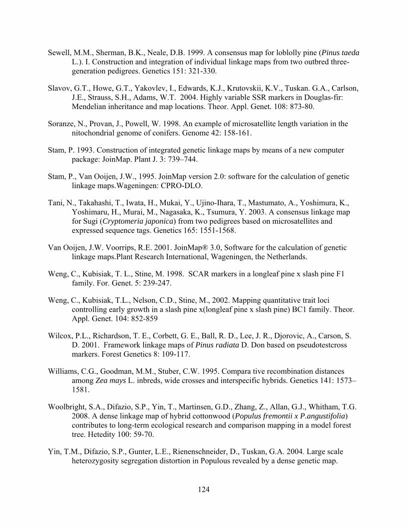
124
Sewell, M.M., Sherman, B.K., Neale, D.B. 1999. A consensus map for loblolly pine (Pinus taeda L.). I. Construction and integration of individual linkage maps from two outbred three-generation pedigrees. Genetics 151: 321-330.
Slavov, G.T., Howe, G.T., Yakovlev, I., Edwards, K.J., Krutovskii, K.V., Tuskan. G.A., Carlson, J.E., Strauss, S.H., Adams, W.T. 2004. Highly variable SSR markers in Douglas-fir: Mendelian inheritance and map locations. Theor. Appl. Genet. 108: 873-80.
Soranze, N., Provan, J., Powell, W. 1998. An example of microsatellite length variation in the nitochondrial genome of conifers. Genome 42: 158-161.
Stam, P. 1993. Construction of integrated genetic linkage maps by means of a new computer package: JoinMap. Plant J. 3: 739–744.
Stam, P., Van Ooijen, J.W., 1995. JoinMap version 2.0: software for the calculation of genetic linkage maps.Wageningen: CPRO-DLO.
Tani, N., Takahashi, T., Iwata, H., Mukai, Y., Ujino-Ihara, T., Mastumato, A., Yoshimura, K., Yoshimaru, H., Murai, M., Nagasaka, K., Tsumura, Y. 2003. A consensus linkage map for Sugi (Cryptomeria japonica) from two pedigrees based on microsatellites and expressed sequence tags. Genetics 165: 1551-1568.
Van Ooijen, J.W. Voorrips, R.E. 2001. JoinMap® 3.0, Software for the calculation of genetic linkage maps.Plant Research International, Wageningen, the Netherlands.
Weng, C., Kubisiak, T. L., Stine, M. 1998. SCAR markers in a longleaf pine x slash pine F1 family. For. Genet. 5: 239-247.
Weng, C., Kubisiak, T.L., Nelson, C.D., Stine, M., 2002. Mapping quantitative trait loci controlling early growth in a slash pine x(longleaf pine x slash pine) BC1 family. Theor. Appl. Genet. 104: 852-859
Wilcox, P.L., Richardson, T. E., Corbett, G. E., Ball, R. D., Lee, J. R., Djorovic, A., Carson, S. D. 2001. Framework linkage maps of Pinus radiata D. Don based on pseudotestcross markers. Forest Genetics 8: 109-117.
Williams, C.G., Goodman, M.M., Stuber, C.W. 1995. Compara tive recombination distances among Zea mays L. inbreds, wide crosses and interspecific hybrids. Genetics 141: 1573–1581.
Woolbright, S.A., Difazio, S.P., Yin, T., Martinsen, G.D., Zhang, Z., Allan, G.J., Whitham, T.G. 2008. A dense linkage map of hybrid cottonwood (Populus fremontii x P.angustifolia) contributes to long-term ecological research and comparison mapping in a model forest tree. Hetedity 100: 59-70.
Yin, T.M., Difazio, S.P., Gunter, L.E., Rienenschneider, D., Tuskan, G.A. 2004. Large scale heterozygosity segregation distortion in Populous revealed by a dense genetic map.

125
Theor.Appl.Genet. 109: 451-463.
Yin, T.M., Difazio, S.P., Gunter, L.E., Rienenschneider, D., Tuskan, G.A. 2004. Large scale heterozygosity segregation distortion in Populous revealed by a dense genetic map. Theor.Appl.Genet. 109: 451-463.
Zamir, C., Tadmor, Y. 1986. Unequal segregation of nuclear genes in plants. Bot. Gaz. 147: 355–358.
Zhang, D.Q., Zhang, Z.Y., Yang, K., Tian, L. 2002. Segregation of AFLP markers in a (Populus tomentosa x P. bolleana) x P. Tomentosa Carr. BC1 family. For. Stud. China. 4: 21–26.

126
CHAPTER 4 QTL MAPPING FOR GENES CONTROLLING EARLY HEIGHT GROWTH IN LONGLEAF PINE
4.1 Introduction
Mapping quantitative trait loci (QTL) is a basic operation for positional cloning and for
application of marker-assisted selection or marker-assisted introgression in genetic
improvements (Darvasi and Soller, 1994). In forest trees, QTLs for different traits, such as wood
quality (Groover et al., 1994; Kumar et al., 2000; Ball, 2001; Sewell et al., 2002; Sheperd et al.,
2002; Brown et al., 2003; Markussen et al, 2003; Pot et al., 2005a 2005b), growth traits
(Bradshaw and Stettler, 1995; Weng et al., 2002; Gwaze et al., 2003;), and adaptative traits
(Hurme et al., 2000; Brendel et al., 2002; Yazdani et al., 2003; Monclus et al., 2005, 2006,
Tschaplinski et al,2006 ) have been detected, showing the usefulness of this approach for
dissecting genomic regions controlling complex traits.
However, the long-lived nature, outbred mating system, and high genetic load have
hampered the development of QTL analysis in forest trees. Plants undergo significant
morphological changes throughout development, and different sets of genes may contribute to
phenotypic variation from the juvenile to mature phases. In a study of mapping wood density in
Eucalyptus (Verhaegen et al., 1997), none of the QTLs detected at one time (18, 24, and 36
months of age) could be repeated throughout the entire experiment, suggesting that different loci
contribute to phenotypic variation during different stages of development. Weng et al. (2002)
showed in Pinus palustris that the variance explained by major QTLs decrease over time,
suggesting the increased complexity of quantitative traits with the aging of the tree. The
contribution of different sets of genes to quantitative variation during development may lead to

127
low powers of detecting QTLs, as a phenotype measured at rotation age essentially represents the
cumulative effect of many distinct genes.
For outcrossing species, the marker-based linkage mapping of QTLs is generally thought
of as requiring an accumulation of data over a number of relatively small half-sib or full-sib
families that together make up the mapping population (Song, J. Z, 1999). With few exceptions
(Brown et al., 2003; Jermstad et al., 2003), the size of segregating populations used in these
studies is often small (90 to 200 individuals). Among factors influencing QTL detection powers,
small sample sizes and low trait heritability were shown to cause an overestimation of QTL
effects, underestimation of QTL number, and hamper the detection of QTLs with low effects
(Beavis 1995). In addition, over the mapping population as a whole, there is a strong tendency
for linkage equilibrium of marker alleles and QTL alleles. Small family size and linkage
equilibrium reduce the power of full-sib and half-sib populations as much as 10-fold compared
with populations derived from crosses between inbred lines (Soller and Genizi, 1978; Weller et
al., 1990; Knott and Haley, 1992; van der Beek et al., 1995; Knott et al., 1996).
Statistical methods are well developed for single-family degrees (Lander and Botstein
1989; Haley and Knott, 1992; Jansen, 1994; Zeng, 1994); however, it is undesirable when the
two lines initiating the cross are not segregating at a QTL (Xu, 1998). If a QTL is present, but
undetected because of fixation to the same allele in both lines, then a type II error, also referred
to as a genetic drift error (Xu, 1996), has occurred. A type II error can be reduced by using
multiple families (Muranty, 1996), and the simulations have shown that six parents should give a
good sample of variance and allow the detection of QTLs with reasonable power if the QTL
heterozygote frequency in the base population is high enough.
128
For these reasons, a single QTL detection experiment in a single-family pedigree with a
small population size does not give an exhaustive idea of the genetic architecture of a
quantitative trait. One possible strategy to overcome these difficulties is to detect QTLs several
times across different families, environments, and developmental stages. In this way, by un-
segregating QTLs, the environmental and temporal stability of QTLs can be verified and a more
complete picture of the genetic architecture of the complex trait can be drawn.
The major objectives for this chapter are to:
1) Analyze the phenotype traits at the different ages and their correlation;
2) Identify the QTLs controlling EHG in longleaf pine.
4.2 Materials and Methods
4.2.1 Plant Materials, DNA Isolation and Gel Electrophoresis
A half-sib family, which included longleaf pine x slash pine hybrid Derr 488 as a
common paternal parent and six longleaf pines as recurrent maternal parents, was selected for the
QTL identification. Within each of the six full-sib families, the tallest and shortest 8% of
seedlings (220 seedlings total) were selected for QTL detection (phase I). Random selections of
8 percent of the seedlings from the rest of the population (110 seedlings) and 25 seedlings from
both tails (135 seedlings total) of the within-family distributions were used for unbiased QTL
verification and mapping (phase II). Due to the DNA isolation failure and the results of mis-
parentage, there were only 305 samples used for the final data analysis (see Chapter 3). One
hundred and sixty (160) samples were used for phase I, consisting of the 85 tallest samples and
the 75 shortest samples. One hundred and seventy (170) samples were used for phase II, which
including 110 random samples from the rest of the population, 30 samples from previous study

129
to make up the losing samples due to mis-parentage, and 25 randomly selected seedlings from
the phase I population.
The DNA isolation, purification, and quantification procedures follow the method
described in Chapter 2.2.2. The marker preparation, PCR reaction condition, and gel
electrophoresis followed the methods described in Chapter2.2.3 and 2.2.4. For a more detailed
description of experimental design and plant material pedigree, see Chapter 2.
4.2.2 Statistical Analysis for Phenotypic Data
In this study, the height and diameter measurements for each year were used as the
response variables to estimate the early height growth of longleaf pine. For each year, a different
plot was assigned, thus, the year effect and the plot effect were confounded. When a plot was
proved to be significant, it was hard to distinguish whether it was caused by the year effect,
location effect, or their interaction. To solve the problem, a new variable called ‘environment’, a
combination of the plot and year effect (i.e., the seven different field tests), was created.
Therefore, the linear model used in the study was
where is the overall mean, is the female parent effect (i=6 for six female parants), is the
environment effect (i=7 for seven different test fields, a combination of year and plot
effect), is the female parent-by-environment interaction, is the replication effect
within each environment, and is the trait value for ith family, jth environment kth
replication and lth tree. The family effect was a fixed effect the environment, the female-by-
environment interaction and replication were treated as the random effect.
All the phenotypic data analyses for the population were performed using SAS (ver 9.1).
The heights and diameters for the entire half-sib families were first tested for normality using the
130
Shappiro-Wilk test (SAS Proc Univariate). The correlations between the 5 traits were tested by
the Pearson test statistic. The ANOVA was performed using PROC MIXED because of the
mixed effects.
The trait value of a tree was determined by the female effect, environment effect,
and their interaction. To reflect the true value of the genetic effect for the tree, a residual value
, was used as a final response value for the QTL analysis. The interaction
between family and environment was tested first. If the interaction was not significant for the
tested trait, the interaction for the trait was dropped from the full model (model 4.1), and the
residual value for that trait included the genetic effect and error term only. If the interaction for a
trait was significant, the residual value then included the genetic effect, the error, and the specific
female-by-environment effect. The residual process was performed with SAS Proc Glm/solution,
which is the regression approach for categorical data. These residual values were used as the trait
value for DNA sample selection for selective genotyping and for QTL mapping.
4.2.3 QTL Identification
Associations between segregating genetic markers and phenotypic traits were detected
using both the single point method and interval mapping method. Since marker-QTL phase
relationships were not known a priori because of linkage equilibrium, and the interactions
among QTL alleles were possibly dependent on the genetic background for each individual
family, the analyses were conducted for each marker in each full-sib family individually by
software MapQTL (ver.4.0). The linkage phase used for each pair of molecular markers was
obtained from JoinMap (ver.3.0) in the process of linkage mapping analyses. However, MapQTL
(ver.4.0) cannot join the data from different families. The significant markers for a QTL
determined by MAPQTL across at least 3 full-sib families were then outputted and re-analyzed
131
by simple regression approach. The regression considered, as the dependent variable, the value
of the measured character in each of the 305 half-sib progenies. As the regressor, the allelic
composition of each SSR locus was used.
Interval mapping was performed by QTL-Express (Seaton et al., 2002), a World Wide
Web-based interface for the least square method (Haley and Knott, 1992; Haley et al, 1994;
Knott et al., 1996) for both the detection population (Phase I) and the verification population
(Phase II). QTL express was the first application for QTL mapping in outbred populations with a
web-based user interface (Seaton, 2002). The analysis was carried out using the half-sib module,
in which QTLs were mapped and explained by within-family variations, with the evidence for
QTL segregation accumulated across the common parents (Knott et.al., 1996). Trait data were
tested for normality using the Shapiro-Wilk test before the QTL identification. Each linkage
group was scanned at 5-cM intervals for locations explaining a high proportion of the phenotypic
variance using a one-QTL model and a two-QTL model. Chromosome-wide permutation tests
with 1000 iterations were carried out to determine P-values and a significant threshold of 0.05
was taken as evidence for the presence of a QTL (Churchill and Doerge, 1994; Seaton, 2002).
The confidence interval (CI) for the position of a QTL was defined as the interval in which the F-
statistics of the presence of a QTL was at least twofold of its maximum value, and the bootstrap
procedure was used to estimate the confidence interval of a QTL location (Visscher et al., 1996).
4.3 Results
4.3.1 Phenotypic Analysis of Height and Diameter
The ANOVA table for the above statistical model is given in Table 4.1. For all 5 traits,
the interaction between family and environment was not significant, except ht2 (p=0.002), while
the environment and female parent effects were all significant (P<0.001). To evaluate the

132
difference among different environments, the mean responses for each full-sib family at different
environments are summarized in Table 4.2. Only the variable ht4 (total height after planting 4
years) was shown here. The mean responses differed significantly among different test
environments, indicating the quantitative inheritance pattern of the EHG. The families Em17 and
Em24 were significantly taller than the other families, indicating that the parents may be
potential candidate parents for improving EHG. Frequency distributions for total heights,
diameters, and their residual values of the Derr488 half-sib family are shown in Figure 4.1 and
Figure 4.2, respectively.
Table 4.1 ANOVA table for different environments for height at age 4 years (ht4)
Effect Num DF Den DF F Value Pr > F
Female 5 1128 7.43 <.0001
Environment 6 1128 5.87 <.0001
Female x Environment 21 1128 1.01 0.4497
Table 4.2 Mean (cm) estimation of the height (ht4) for individual full-sib family at different environments after being planted for four years
LA MS
Year2002 Year2003 Year2002 Year2003 Environment
FT_1 488_1 FT_2 FT_1 488_1 FT_2 488_2
Em04 222.5 / 193.86 187.83 / 162.52 188.85 186.17
Em14 181.5 176.78 175.06 187.07 132.07 146.17 162.22 162.74
Em17 183.13 204.65 213.62 268.22 206.25 176.1 202.83 203.57
Em24 202.91 196.81 245.83 203.96 164.35 187.52 203.45 197.95
Em41 150.57 169.07 / 159.6 / / / 164.82
Em45 187.87 196.29 / 224.44 150.48 / / 185.58
Over Females 180.95 185.30 209.32 206.91 159.26 171.27 187.44
185.92
Note: / there are no progenies presented for the sites.
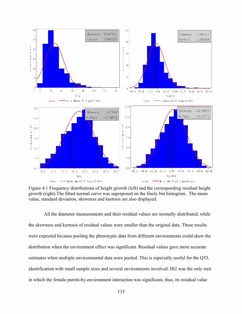
133
Figure 4.1 Frequency distributions of height growth (left) and the corresponding residual height growth (right).The fitted normal curve was superposed on the finely bin histogram. The mean value, standard deviation, skewness and kurtosis are also displayed.
All the diameter measurements and their residual values are normally distributed, while
the skewness and kurtosis of residual values were smaller than the original data. These results
were expected because pooling the phenotypic data from different environments could skew the
distribution when the environment effect was significant. Residual values gave more accurate
estimates when multiple environmental data were pooled. This is especially useful for the QTL
identification with small sample sizes and several environments involved. Ht2 was the only trait
in which the female parent-by-environment interaction was significant, thus, its residual value

134
included both within family genetic effect and genetic by specific site interaction. This may help
to explain why ResHt2 was not normally distributed. The parent by environment interactions for
other traits were not significant, thus the interaction term was dropped from the full model and
residual value for these traits, included only genetic effects and random error. For the QTL
analyses, the residual values for all phenotypic traits were used instead of the original value. The
original data were used for identifying QTL by environment interaction.
Figure 4.2 Frequency distributions of diameter (left) and the corresponding residual diameter (right). The fitted normal curve was superpose on the finely bin histogram. The mean value, standard deviation, skewness and kurtosis are also displayed.
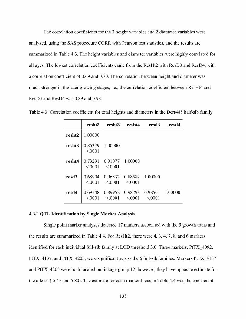
135
The correlation coefficients for the 3 height variables and 2 diameter variables were
analyzed, using the SAS procedure CORR with Pearson test statistics, and the results are
summarized in Table 4.3. The height variables and diameter variables were highly correlated for
all ages. The lowest correlation coefficients came from the ResHt2 with ResD3 and ResD4, with
a correlation coefficient of 0.69 and 0.70. The correlation between height and diameter was
much stronger in the later growing stages, i.e., the correlation coefficient between ResHt4 and
ResD3 and ResD4 was 0.89 and 0.98.
Table 4.3 Correlation coefficient for total heights and diameters in the Derr488 half-sib family
resht2 resht3 resht4 resd3 resd4
resht2 1.00000
resht3 0.85379<.0001
1.00000
resht4 0.73291<.0001
0.91077<.0001
1.00000
resd3 0.68904<.0001
0.96832<.0001
0.88582<.0001
1.00000
resd4 0.69548<.0001
0.89952<.0001
0.98298<.0001
0.98561<.0001
1.00000
4.3.2 QTL Identification by Single Marker Analysis
Single point marker analyses detected 17 markers associated with the 5 growth traits and
the results are summarized in Table 4.4. For ResHt2, there were 4, 3, 4, 7, 8, and 6 markers
identified for each individual full-sib family at LOD threshold 3.0. Three markers, PtTX_4092,
PtTX_4137, and PtTX_4205, were significant across the 6 full-sib families. Markers PtTX_4137
and PtTX_4205 were both located on linkage group 12, however, they have opposite estimate for
the alleles (-5.47 and 5.80). The estimate for each marker locus in Table 4.4 was the coefficient
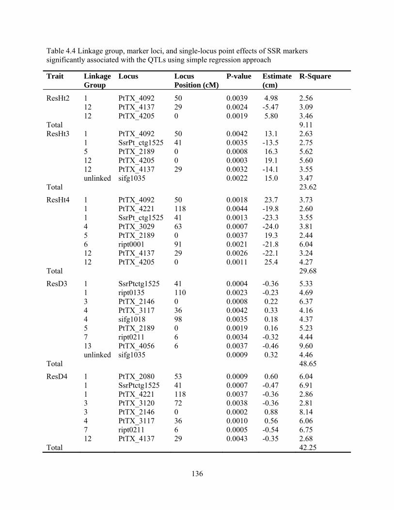
136
Table 4.4 Linkage group, marker loci, and single-locus point effects of SSR markers significantly associated with the QTLs using simple regression approach
Trait Linkage Group
Locus Locus Position (cM)
P-value Estimate (cm)
R-Square
ResHt2 1 PtTX_4092 50 0.0039 4.98 2.56 12 PtTX_4137 29 0.0024 -5.47 3.09 12 PtTX_4205 0 0.0019 5.80 3.46 Total 9.11 ResHt3 1 PtTX_4092 50 0.0042 13.1 2.63 1 SsrPt_ctg1525 41 0.0035 -13.5 2.75 5 PtTX_2189 0 0.0008 16.3 5.62 12 PtTX_4205 0 0.0003 19.1 5.60 12 PtTX_4137 29 0.0032 -14.1 3.55 unlinked sifg1035 0.0022 15.0 3.47 Total 23.62
ResHt4 1 PtTX_4092 50 0.0018 23.7 3.73 1 PtTX_4221 118 0.0044 -19.8 2.60 1 SsrPt_ctg1525 41 0.0013 -23.3 3.55 4 PtTX_3029 63 0.0007 -24.0 3.81 5 PtTX_2189 0 0.0037 19.3 2.44 6 ript0001 91 0.0021 -21.8 6.04 12 PtTX_4137 29 0.0026 -22.1 3.24 12 PtTX_4205 0 0.0011 25.4 4.27 Total 29.68
ResD3 1 SsrPtctg1525 41 0.0004 -0.36 5.33 1 ript0135 110 0.0023 -0.23 4.69 3 PtTX_2146 0 0.0008 0.22 6.37 4 PtTX_3117 36 0.0042 0.33 4.16 4 sifg1018 98 0.0035 0.18 4.37 5 PtTX_2189 0 0.0019 0.16 5.23 7 ript0211 6 0.0034 -0.32 4.44 13 PtTX_4056 6 0.0037 -0.46 9.60 unlinked sifg1035 0.0009 0.32 4.46 Total 48.65
ResD4 1 PtTX_2080 53 0.0009 0.60 6.04 1 SsrPtctg1525 41 0.0007 -0.47 6.91 1 PtTX_4221 118 0.0037 -0.36 2.86 3 PtTX_3120 72 0.0038 -0.36 2.81 3 PtTX_2146 0 0.0002 0.88 8.14 4 PtTX_3117 36 0.0010 0.56 6.06 7 ript0211 6 0.0005 -0.54 6.75 12 PtTX_4137 29 0.0043 -0.35 2.68 Total 42.25

137
estimate differences between the two alleles for common parent Derr488. Since the linkage
phase of markers and QTLs was not known priori, the estimate was simply the mean differences
between two alleles (smaller allele size vs larger allele size) of the associated marker. There are 6
markers identified as associated with ResHt3. Among these markers, two of them were located
on linkage group 1 and two markers were located on linkage group 12. An unlinked marker,
sifg1035, was also found to associate with ResHt3. Eight markers were identified for ResHt4:
three of them were located on linkage group 1, two markers were located on linkage group 12,
three markers were scattered on linkage groups 4, 5, and 6, and one unlinked marker, sifg1035,
was also identified. Three markers PtTX_4092, PtTX_4137, and PtTX_4205 were linked with all
of the height growth traits.
Nine and eight markers were identified to associate with ResD3 and ResD4, respectively.
The markers linked to ResD3 were distributed in 6 linkage groups and the unlinked marker
sifg1035 was also linked to the trait. The markers associated with trait ResD4 were distributed in
5 linkage groups. The marker SsrPtctg1525 was found to associate with 4 of the interested traits
(ResHt3, ResHt4, ResD3, and ResD4). Marker PtTX_4092 was only linked to those height traits
and markers PtTX_2146 and PtTX_3117 were only associated with diameter traits. Most of the
markers were distributed on linkage groups 1, 5, 7, and 12.
For the simple marker approach, the software MapQTL (ver 4.0) was first explored to
identify the markers associated with the QTLs. Since the software does not handle the linkage
data from different parents, and cannot combine the linkage information from multiple families,
the significant markers were output and re-analyzed by SAS regression. Therefore, two-phase
strategy was not performed for single marker approach due to small sample size within each full-
sib family.

138
4.3.3 Phase I: QTL Detection by Interval Mapping
The QTL identification by interval mapping was following a two-phase strategy: QTL
detection by selective genotyping and QTL verification by random sampling. For Phase I, 18
QTLs were detected for 5 traits by QTL express and were located in 8 intervals (Table 4.5).
Table 4.5 Intervals detected that contain QTLs influencing growth traits by QTL Express for QTL detection population L.G Trait Position
(cM)
Interval CI
(cM)
Est. P value Variation
1 ResHt2 40 ript0031-SsrPtctg1525 7.83 0.0111
ResHt2 120 PtTX_4221-ript0225 10-124 14.52 0.0032 7.55%
ResHt3 40 ript0031-SsrPtctg1525 2-125 -40.12 0.0088 3.01%
ResHt4 40 ript0031-SsrPtctg1525 24-124 -65.78 0.0072 3.22%
ResD3 35 ript0031-SsrPtctg1525 12-50 -0.74 0.0085 2.86%
ResD4 115 ript0135-PtTX_4221 88-124 0.90 0.0093 2.92%
2 ResHt3 5 sifg1052-sifg1064 0-15 27.26 0.0125 2.60%
ResHt4 5 sifg1052-sifg1064 0-12 38.38 0.0188 2.13%
ResD3 5 sifg1052-sifg1064 0-18 0.57 0.0115 2.68%
4 ResHt4 80 sifg1060-ript0287 75-95 -39.45 0.0089 3.01%
ResD4 80 sifg1060-ript0287 75-95 -0.79 0.0091 3.01%
7 ResHt2 75 ript9104-PtTX_4130 60-110 12.93 0.0018 4.85%
ResHt3 75 ript9104-PtTX_4130 65-110 33.31 0.0028 4.30%
ResHt4 75 ript9104-PtTX_4130 60-110 69.85 0.0011 4.92%
ResD3 75 ript9104-PtTX_4130 60-110 1.01 0.0045 3.76%
ResD4 75 ript9104-PtTX_4130 60-110 1.16 0.0022 4.42%
12 ResHt4 0 PtTX_4205-ript0852 0-28 -11.07 0.0014 5.22%
ResHt4 25 RPTest01-PtTX_4137 0-28 38.16 0.0009 6.87%
L.G.: linkage group; Position (cM): position to which the QTL mapped in cM; Variation: percentage variation explained by the QTL; CI: confidence interval; P-value: significance of a quantitative trait locus being present; Est.: The estimation of QTL effect.
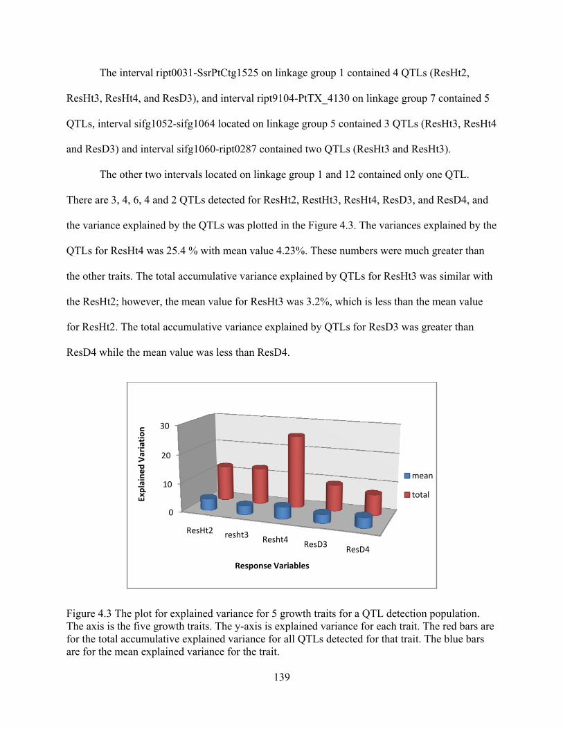
T
ResHt3, R
QTLs, in
and ResD
T
There are
the varian
QTLs for
the other
the ResH
for ResH
ResD4 w
Figure 4.The axis for the toare for th
The interval r
ResHt4, and
nterval sifg10
D3) and inter
The other two
e 3, 4, 6, 4 an
nce explaine
r ResHt4 wa
r traits. The t
Ht2; however
Ht2. The total
while the mea
.3 The plot fis the five g
otal accumulhe mean expl
Explaine
d Variation
ript0031-Ssr
d ResD3), an
052-sifg1064
rval sifg1060
o intervals lo
nd 2 QTLs d
ed by the QT
as 25.4 % wi
total accumu
r, the mean v
l accumulati
an value was
for explainedgrowth traits.ative explainlained varian
0
10
20
30
ResHt2
rPtCtg1525 o
nd interval ri
4 located on
0-ript0287 c
ocated on lin
detected for
TLs was plot
ith mean valu
ulative varian
value for Res
ive variance
s less than R
d variance fo. The y-axisned variancence for the tr
2 resht3 R
Respon
139
on linkage g
ipt9104-PtTX
n linkage gro
contained tw
nkage group
ResHt2, Res
tted in the Fi
ue 4.23%. T
nce explaine
sHt3 was 3.2
explained b
ResD4.
or 5 growth tis explained
e for all QTLrait.
Resht4 Res
se Variables
roup 1 conta
X_4130 on l
oup 5 contain
wo QTLs (Re
1 and 12 co
stHt3, ResHt
igure 4.3. Th
These numbe
ed by QTLs f
2%, which is
y QTLs for
traits for a Qd variance foLs detected f
sD3 ResD4
ained 4 QTL
linkage grou
ned 3 QTLs
sHt3 and Re
ntained only
t4, ResD3, a
he variances
ers were muc
for ResHt3 w
s less than th
ResD3 was
QTL detectioor each trait. for that trait.
4
me
tot
Ls (ResHt2,
up 7 containe
(ResHt3, Re
esHt3).
y one QTL.
and ResD4, a
explained b
ch greater th
was similar w
he mean valu
greater than
n populationThe red bar The blue ba
ean
tal
ed 5
esHt4
and
by the
an
with
ue
n. s are ars

140
The QTL interval peaks for all traits at each linkage group are also plotted in Figure 4.4
for graphically review of the QTLs. Two QTL peaks were found on linkage group 1 (Picture A).
One peak was located around 40 cM and the other peak was around 120 cM. All traits except
ResD5 reached the significant F threshold 5.8 at the QTL peak 40 cM. However, for the second
peak 120 cM, only two traits, ResHt2 and ResD4, reached the F threshold. Picture B is for
linkage group 2. There is only one peak at 0-5 cM and three traits ResHt3, ResHt4 and ResD3
reached the significant F threshold 4.3. For the linkage group 4 (Picture C) , there is one QTL
peak located at 80 cM, two traits ResHt4 and ResD4 reached the F threshold 4.5. One QTL peak
is also found for linkage group 7 (Picture D) and all traits are significant. Two QTL peaks are
found for linkage group 12, and only trait ResHt4 was significant at both peaks.
4.3.4 Phase II: QTL Verification by Interval Mapping
In phase II, 15 QTLs were identified at 8 intervals distributed on 6 linkage groups (Table
4.6) and the accumulative explained variation for each trait was plotted in Figure 4.5. Compared
with the results from Phase I, the QTL verification population failed to detect any QTLs on
linkage group 2, while QTLs were verified on linkage groups 4, 7, and 12 with some light
change on location, and new QTLs were identified on linkage groups 5 and 6. The QTLs
detected included 3 QTLs for ResHt2, 2 QTLs for ResHt3, 4 QTLs for ResHt4, 3 QTLs for
ResD3, and 3 QTLs for ResD4. The Over-plot for QTLs identified for each linkage group is
shown in Figure 4.6. For picture A, the peak at 40 cM contained 5 QTLs for each studied trait
and a second peak at 120 cM for ResHt2, but failed to verify the ResD4 at this position. For
linkage group 4, only the QTLs for ResHt4 were verified, and for linkage group 12, both ResHt3
and ResHt4 were verified. The accumulative explained variance for height growth was decreased
from ResHt2 to ResHt3, while increased for ResHt4. The explained variance from ResD3 and

141
Figure 4.4 The overplot of QTLs for growth traits detected by interval mapping with QTL Express for QTL detection population. The X-axis is the position of linkage group with cM as the unit. The Y-axis is the F test value for each trait. The different colors of the plots are for different traits. A: linkage group 1, B: linkage group 2, C: linkage group 4, D: linkage group 7 and E: linkage group 12.
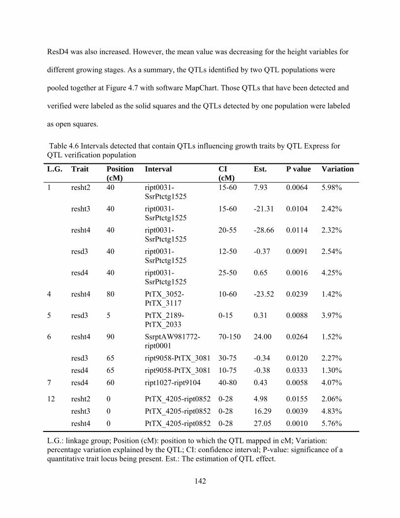
142
ResD4 was also increased. However, the mean value was decreasing for the height variables for
different growing stages. As a summary, the QTLs identified by two QTL populations were
pooled together at Figure 4.7 with software MapChart. Those QTLs that have been detected and
verified were labeled as the solid squares and the QTLs detected by one population were labeled
as open squares.
Table 4.6 Intervals detected that contain QTLs influencing growth traits by QTL Express for QTL verification population
L.G. Trait Position (cM)
Interval CI (cM)
Est. P value Variation
1 resht2 40 ript0031-SsrPtctg1525
15-60 7.93 0.0064 5.98%
resht3 40 ript0031-SsrPtctg1525
15-60 -21.31 0.0104 2.42%
resht4 40 ript0031-SsrPtctg1525
20-55 -28.66 0.0114 2.32%
resd3 40 ript0031-SsrPtctg1525
12-50 -0.37 0.0091 2.54%
resd4 40 ript0031-SsrPtctg1525
25-50 0.65 0.0016 4.25%
4 resht4 80 PtTX_3052-PtTX_3117
10-60 -23.52 0.0239 1.42%
5 resd3 5 PtTX_2189-PtTX_2033
0-15 0.31 0.0088 3.97%
6 resht4 90 SsrptAW981772-ript0001
70-150 24.00 0.0264 1.52%
resd3 65 ript9058-PtTX_3081 30-75 -0.34 0.0120 2.27% resd4 65 ript9058-PtTX_3081 10-75 -0.38 0.0333 1.30% 7 resd4 60 ript1027-ript9104 40-80 0.43 0.0058 4.07%
12 resht2 0 PtTX_4205-ript0852 0-28 4.98 0.0155 2.06% resht3 0 PtTX_4205-ript0852 0-28 16.29 0.0039 4.83% resht4 0 PtTX_4205-ript0852 0-28 27.05 0.0010 5.76%
L.G.: linkage group; Position (cM): position to which the QTL mapped in cM; Variation: percentage variation explained by the QTL; CI: confidence interval; P-value: significance of a quantitative trait locus being present. Est.: The estimation of QTL effect.

Figure 4.The axis for the toare for th
4.4 Discu
4.4.1 Phe
F
genetics
adaptive
populatio
envrionm
environm
environm
know wh
effect. If
.5 The plot fis the five g
otal accumulhe mean expl
ussion
enotypic Da
orest tree br
(Zobel and T
characters, a
on in each en
ment were po
ment effect w
ment effect, t
hether it caus
f the samples
Explaine
d Variance
for explainedgrowth traits.ative explainlained varian
ata
reeding tradi
Talbert 1984
are quantitat
nvironment i
ooled togethe
was significa
that is, when
sed by the ge
s were select
0
2
4
6
8
10
12
ResHt2
d variance fo. The y-axisned variancence for the Q
tionally has
4). Most com
tive and tend
in this study
er, they tend
ant. Thus, the
n a seedling w
enetic effect
ted by origin
2 ResHt3 R
Respon
143
or 5 growth tis explained
e for all QTLQTLs.
been viewed
mmercially im
d to normal d
y. However, w
ded to be bi-m
e genetic eff
was identifie
t or was just
nal data, mos
ResHt4 ResD
se Variable
traits for QTd variance foLs detected f
d as an appli
mportant tra
distribution.
when the tre
modal or ske
fect was conf
ed as an extr
the response
st upper extr
D3 ResD4
TL detection or each trait. for that trait.
ication of qu
aits, such as g
This is true
ees from diff
ewed becaus
founded with
reme sample
e to certain e
reme sample
mea
var
population. The red bar The blue ba
uantitative
growth and
for the tree
ferent
se the
h the
, we do not
environment
s would com
an
s are ars
tal
me

144
Figure 4.6 The overplot of QTLs for growth traits detected by interval mapping with QTL Express for QTL verification population. The X-axis is the position of linkage group with cM as unit; the Y-axis is the F test value for each trait. The different colors of the plots are for different for different traits. A: linkage group 1, B: linkage group 4, C: linkage group 5, D: linkage group 6, E: linkage group 7, and F: linkage group 12.

145
Figure 4.7 The QTLs were detected and verified by 3 populations and 2 methods at different linkage groups. The red color is for ResHt2, the dark green color is for the ResHt3, the Brown color is for ResHt4, the pink color is for ResD3, and the light green color is for ResD4. The solid squares with color filled in are the QTLs detected and verified by all populations and methods. The open squares without filled color are the QTLs detected by the single point method and interval mapping for QTL detection populations, but were not verified. The lines on each square are the confidence intervals for each identified QTL.
146
from LAFT_2 and lower extreme samples would come from MS488_1. When the
environmental effect was accounted for in the phenotypic data, the environment effect for the
residual value was not significant (p=0.39), and the residual value for all environments was
comparable. Therefore, all the trait values from different environments can be pooled
together for data analysis without inflated error.
A simulation test showed that the required sample size would be 800 if two genotypes
and three environments were involved (Weng, 1999). In this study, the sample size for each
QTL identification population was less than 200 and 7 environments, 5 traits were involved.
The QTL power would be extremely small when the original data was explored. Accordingly,
using the residual value would a useful solution to reduce error and increase power.
4.4.2 QTL Methods and Statistical Techniques
Two QTL methods were performed for identifying the QTLs association with early
height growth in longleaf x slash pine: the single marker method and the interval method.
One advantage of single marker analyses is it can identify the association between QTLs and
unlinked markers, e.g. sifg1035 in this study, since it does not require a genetic map. In a
sufficient marker-saturated map region (Darvasi et al., 1993) or in designs where
recombination has been limited, single marker testing is as good as any other method for
finding QTLs one at a time. However, a major disadvantage for the single marker test is that
the QTL effect and the location are confounded, and unable to be estimated separately. Hence,
the single maker method was used as a rough estimate of QTL location and searches the
QTLs for unlinked markers in this study.
Compared to the method of single marker analyses, interval mapping methods have
been shown to be more powerful, accurate, and robust to the failure of normality assumption
(Lander and Botstein, 1989; Knott and Haley, 1992). The original method implemented in
interval mapping was maximum likelihood (ML) in which information on the presence of a

147
QTL was derived from both the mean difference between the flanking marker genotype
classes and the distribution of the trait within each marker genotype class. In 1995, a
qualitatively different approach was adapted by Xu and Atchley from a method of human
genetics that requires only the estimation of the identity-by-descent (IBD) proportion of
alleles shared by pairs of individuals at a map position. For a QTL at this position, high IBD
should be accompanied by low phenotypic difference. Such a “random model” algorithm,
which models the variance rather than the magnitude of QTL effects, has been implemented
for plant and animal designs in the web-based software QTL Express. In outbreeding species,
marker-QTL phase relationships are not known a priori because of linkage equilibrium. Its
advantage over “fixed model” methods are that it requires no knowledge of linkage phase or
number of alleles at loci and is readily adapted to complicated pedigree designs (Nelson
2005). At a QTL position, simple regression of phenotypic value on the expectation of the
genotype given flanking markers, expressed in the term of additive effect “α” and dominance
“d”, lead to estimates of these effects (Haley and Knott, 1992; Martínez and Curnow 1992).
This method was then extended to outbreeding designs by Haley (1994) and was adapted by
QTL Express.
In the process of interval mapping, only the regions of the genome that exceed
chromosome wide P<0.05 were reported. Empirically derived significance thresholds for all
traits from 1,000 permutations were found to be quite similar (data not shown) for a given
chromosome. Therefore, the same threshold was used for all traits on a given chromosome.
As suggested by Thomsen et al. (2004) for the parent of origin models, significance tests with
the same degrees of freedom had similar significance thresholds, so empirically derived
thresholds for 1-QTL vs. no QTL were used for 2-QTL vs. 1-QTL. In addition to
chromosome-wise significance thresholds, experiment-wise significance thresholds were also
obtained by the option of an experimental-wide module in QTL Express (de Koning et al.,
148
2001). The threshold obtained by chromosome-wide P<0.05 (suggestive level) and P<0.01
(significantly level) correspond approximately to experimental-wide significant levels of 0.6
and 0.12, respectively, following by the Bonferroni correction (Lynch and Walsh, 1998).
Therefore, it is possible that some QTLs identified by chromosome-wide threshold are false
positive, but are reported to the mapping community as recommended by Lander and
Kruglyak (1995).
4.4.3 QTL Detection Population and Verification Population
QTL location by whatever method involves scanning each chromosome for the most
likely position of the QTL. This inevitably implies that a large number of possible positions
are tested and those whose likelihood of containing a QTL exceeds some critical value are
accepted. To avoid too many false positives, the test probability level is adjusted downwards
to allow for the multiple tests, and obviously, this has the concomitant result of increasing the
probability of false negatives. The only real solution to the problems of QTL location in
segregating populations is to repeat experiments using a completely different sample of
genotypes derived from the same population. Thus, two phases of QTL identification strategy
was used in this study.
After the QTLs were detected by the first population, another QTL identification
procedure was then performed for verifying whether there are QTLs in the second population
located at the position identified in the first. Using more than a single family for QTL
mapping may reduce a type II error caused by homogeneous parents being sampled. This
strategy was also applied by Groover et al., (1994), Knott et al., (1997), Sewell et al., (2000,
2002), and Brown et al.,(2003) in early QTL mapping studies for wood quality in loblolly
pine. Devey et al. (2004) also used 6 related radiata pine full-sib families to detect and
independently verify QTLs for resistance to Dothistroma needle blight.

149
In the QTL detection population (Phase I), a non-random selection of samples can
increase the statistical power for detecting QTLs responsible for the trait used as the selection
criterion. However, caution must be taken about the statistical inference space of the
parameter estimation. Because of the non-random selection, estimation of the QTL effect is
biased, can only be inferred upon the selective trait, and may not be helpful in detecting
QTLs responsible for other traits. The residual value of Ht3 was used as the criterion for
selective genotyping. The correlation test of the trait has shown that ResHt3 has high
correlation with all the other traits, which may reduce the inaccuracy of detecting QTLs on
other traits. Verification of QTL was based on the repeated detection of QTL among
populations, as well as among multiple growing seasons for each population (Brown et al.,
2003). In the study, a randomly selected sample was used as the non-biased verification
population. Compared with the bi-modal distribution of the phase I populations, all the traits
for the QTL verification population were normally distributed. Also since the verification
population do not infer upon any specific traits, the power of QTL identification for all traits
were the same. Therefore, the QTL verification is essential to substantiate a biological basis
for observed marker-trait association, to provide precise estimates of the magnitude of QTL
effects, and to predict whether a QTL will be expressed at a given developmental age (Brown,
et al., 2003).
However, give the allogamous reproductive system and recent domestication, pines
are characterized by high levels of genetic diversity and low level of linkage disequilibrium
(LD) (Reviewed by Gonzάlez-Martinez et al 2006). Together with its perennial
characteristics, pines are generally assumed to contain QTL with low stability across
genotypes and environments. In this study, only small fraction (33%) of the detected QTLs is
common across two populations. This phenomenon was also reported by Brown et al. (2003)

150
and Devey et al. (2004 a, b). An unusual observation made by Kaya et al. (1999) was a failure
to find any QTLs shared between pedigrees.
4.4.4 QTLs Associated with Growth Traits
In the QTL detection population, 3 QTLs were detected for association with ResHt2
and explained 12.4% of the phenotypic variance, in which 2 QTLs were located on linkage
group 1, and 1 QTL was located on linkage group 7. In the QTL verification population, two
QTLs located on linkage group 1 were verified, while the QTLs located on linkage group 7
failed the verification. Instead, a QTL located on linkage group 12 was found to be associated
with ResHt2 in verification population and the 3 QTLs explained 8.04% of the phenotypic
variance. This result from QTL verification population was similar to the results from single
marker regression. From Figure 4.4 E, I found there was a peak for all traits at the marker
interval PtTX_4205-ript0852 on linkage group 12 for QTL detection population. However,
only the QTL for ResHt4 have reached the criterion value, and as seen in figure 4.6 F, all the
height growth traits have reached the criterion. The different QTLs identified from different
families were observed in other research (Devey et al., 2004a, 2004b, Kaya et al., 1999). In
this research, the QTL peaks for ResHt2 existed for both populations on linkage groups 7 and
12, while the test statistic was not significant and did not reach the chromosome-wide
criterion, although it was very close to the criterion. It is possible that potential QTLs exsited
at these locations. A similar pattern was also found for other traits. This may be related to the
small sample size used in our study and relatively low heritability of EHG. Beavis (1995)
found that among factors influencing QTL detection powers, small sample sizes (less than
200) and low trait heritability were shown to cause an overestimation of QTL effects,
underestimation of QTL number, and hamper detection of QTLs with low effects (Soller and
Genizi, 1978; Weller et al., 1990; Knott and Haley, 1992; van der Beek et al., 1995; Knott et

151
al., 1996). In this study, 305 backcross progenies were used for QTL identification, but they
were split into two QTL populations, which lead to less than 200 samples for each population.
Weng et al. (2002) found that the variance explained by major QTLs decrease over
time, suggesting the increased complexity of quantitative traits with the aging of the tree.
However, in this study, opposite results were observed for height growth. In both populations,
both the accumulative variance explained by QTL and the mean value for later height growth
(i.e. ResHt4) were greater than those in early height growth (ResHt2 and ResHt3). It may
have been caused by increased numbers of QTLs for the later growth trait in this study. In
Weng’s study, the QTLs identified were 3, 1, and 1 for each height growth variable, while in
this study, numbers of QTLs identified for were 3, 4, and 6 for QTL detection population and
3, 2, and 4 for QTL verification population. Another reason for these results may have been
caused by the environmental stress. Most measurements of Ht4 and D4 in our QTL
population were taken at Year 2006, which was the year after Hurricane Katrina (Year 2005).
During Katrina, many trees were bent and broken (Figure 4.7) and it was possible that some
genes were activated during the recovery process under the growing stress. There was only
weak evidence of QTL stability during the three years of growth under this study. Individual
QTLs became active at various stages. However, some consistency (i.e. the interval ript0031-
SsrPtCtg 1525) was observed for QTLs involved in both height growth and diameter growth,
which was active at the 2nd year and still detectable at the 4th year and was potentially a
major effect gene controlling EHG. Gwaze et al. (2003) also reported the detection of a
similar QTL region at different maturation stages in loblolly pine. However, the ontogenenic
effects is a more common phenomena in pines (Plomion, et al., 1996; Emebiri, et al., 1997;
Sewell et al., 2000; Pot et al., 2004) suggests different genomic regions control the
quantitative traits and explain the low QTL stability across the matuartion stage.
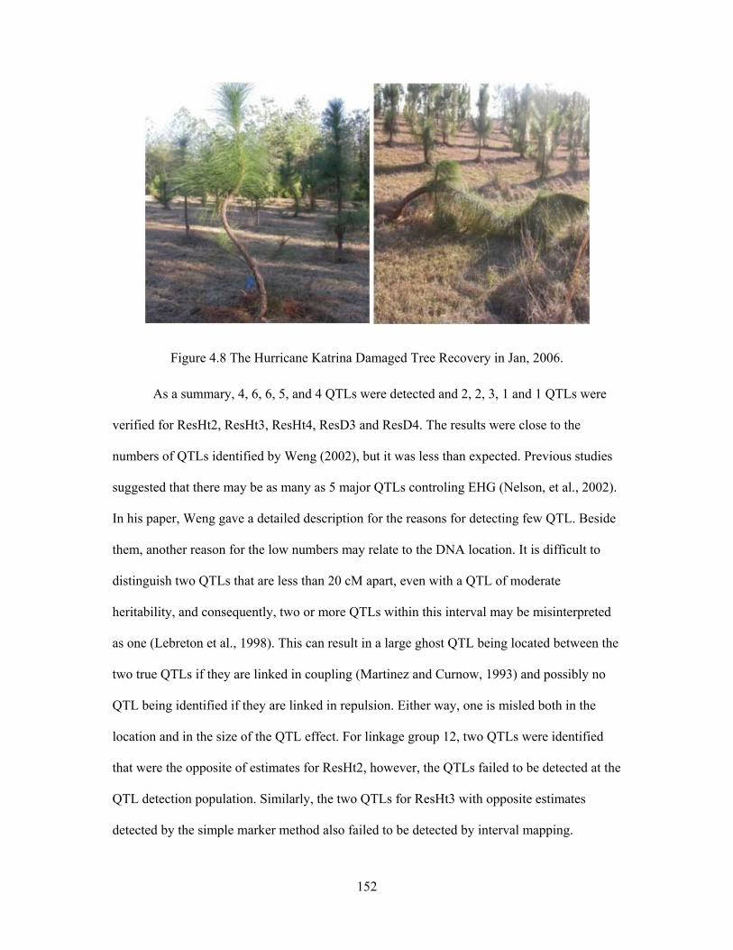
152
Figure 4.8 The Hurricane Katrina Damaged Tree Recovery in Jan, 2006.
As a summary, 4, 6, 6, 5, and 4 QTLs were detected and 2, 2, 3, 1 and 1 QTLs were
verified for ResHt2, ResHt3, ResHt4, ResD3 and ResD4. The results were close to the
numbers of QTLs identified by Weng (2002), but it was less than expected. Previous studies
suggested that there may be as many as 5 major QTLs controling EHG (Nelson, et al., 2002).
In his paper, Weng gave a detailed description for the reasons for detecting few QTL. Beside
them, another reason for the low numbers may relate to the DNA location. It is difficult to
distinguish two QTLs that are less than 20 cM apart, even with a QTL of moderate
heritability, and consequently, two or more QTLs within this interval may be misinterpreted
as one (Lebreton et al., 1998). This can result in a large ghost QTL being located between the
two true QTLs if they are linked in coupling (Martinez and Curnow, 1993) and possibly no
QTL being identified if they are linked in repulsion. Either way, one is misled both in the
location and in the size of the QTL effect. For linkage group 12, two QTLs were identified
that were the opposite of estimates for ResHt2, however, the QTLs failed to be detected at the
QTL detection population. Similarly, the two QTLs for ResHt3 with opposite estimates
detected by the simple marker method also failed to be detected by interval mapping.

153
As discussed in Chapter 3, the integrated linkage map used in QTL identification has
discrepancies with the linkage map built by Echt et al. (In preparation) for loblolly pine.
Given the acknowledged genetic conservation between these two closely related pine species,
further studies are needed before these QTLs can be applied to MAS.
4.5 References
Ball, R.D. 2001. Beyesian methods for quantitative trait loci mapping based on model selection: Approximate analysis using the Bayesian Information Criterion. Genetics 159: 1351-1364.
Beavis, W.D. 1995. The power and deceit of QTL experiments: lessons from comparative QTL studies. In: Proceedings of the Forty-ninth Annual Corn and Sorghum Industry Research Conference, ASTA, Washington, DC. pp. 252–268.
Bradshaw, Jr. H.D., Stettler, R.F. 1995. Molecular genetics of growth and development in Populus. IV. Mapping QTLs with large effect on growth, form and phenology traits in a forest tree. Genetics 139: 963-973.
Brendel, O., Pot, D., Plomion, C., Rozenber, P., Guehl, J.M. 2002. Genetic parameters and QTL analysis of ä13C and ring width in maritime pine. Plant Cell Environ. 25: 945-953.
Brown, G.R., Bassoni, D.L. , Gill, G.P., Fontana, J.R., Wheeler, N.C., Megraw, R.A., Davis, M.F., Sewell, M.M., Tuskan, G.A. Neale, D.B. 2003. Identification of Quantitative Trait Loci Influencing Wood Property Traits in Loblolly Pine (Pinus taeda L.). III. QTL Verification and Candidate Gene Mapping. Genetics 164: 1537–1546.
Churchill, G.A. Doerge, R.W. 1994. Empirical threshold values for quantitative trait mapping. Genetics 138: 963-971.
Darvasi, A., Soller M. 1994. Selective DNA pooling for determination of linkage between a molecular marker and a quantitative trait locus. Genetics 138: 1365-1373.
Darvasi, A., Weintreb, A., Minke, V., Weller, S., Soller, M. 1993. Detecting marker QTL linkage and estimating QTL gene effect and map location using a saturated genetic map. Genetics 134: 943-951.
De Koning, D.J., Rattink, A.P., Harlizius, B., Van Arendonk, J.A.M., Brascamp, E.W. Groenen, M.A.M. 2001. Detection and characterization of quantitative trait loci for meat quality traits in pigs. J. Anim. Sci. 79: 2812-2819.
Devey, M.E., Groom, K.A., Nolan, M.E., Bell, J.C., Dudzinski, M.J., Old, K.M. Matheson, A. C., Moran, G.F. 2004. Detection and verification of quantitative trait loci for resistance to dothistroma needle blight in Pinus radiate. Theor. Appl. Genet.108: 1056-1063.
Echt, C.S., Saha, S., Krutovsky, K., Erpelding, J., Nelson, C.D. Microsatellite-based genetic

154
map for loblolly pine. In preparation.
Groover, A., Devey, M., Fiddler, T., Lee, J., Megraw, R. 1994. Identification of quantitative trait loci influencing wood specific gravity in an outbred pedigree of loblolly pine. Genetics 138: 1293-1300.
Gwaze D.P., Zhou, Y., Reyes-Valdes M.H., Al-Rababah, M.A., Williams, C.G. 2003. Haplotypic QTL mapping in an outbred pedegree. Genet. Res. 81: 43-50.
Haley, C.S., Knott, S.A. 1992. A simple regression method for mapping quantitative trait loci in line crosses using flanking markers. Heredity 69: 315-324.
Haley, C.S., Knott, S.A., Elsen, J-M. 1994. Mapping quantitative trait loci in crosses between outbred lines using least squares. Genetics 136: 1195-1207.
Hurme, P., Sillapaa, M.J., Arjas, E., Repo, T., Savolainen, O. 2000. Genetic basis of climatic adaptation in scots pine by Bayesian quantitative trait locus analysis. Genetics 156: 1309-1322.
Jansen, R.C. Stam, J. 1994. High resolution of quantitative traits into multiple loci via interval mapping. Genetics 136: 1447-1455.
Jermstad, K.D., Bassoni, D.L., Jech, K.S., Ritchie, G.A. Wheeler, N.C. 2003 Mapping of quantitative trait loci controlling adaptive traits in coastal Douglas-fir: III. QTL by environment interactions. Genetics 165: 1489–1506.
Kaya, Z., Sewell, M.M., Neale. D.B., 1999. Identification of QTLs influencing the annual height and diameter increments in loblolly pine (Pinus taeda L.). Theor. Appl. Genet. 98: 586-592.
Knott, S.A., Haley, C.S. 1992. Maximum likelihood mapping of quantitative traits loci using full-sib families. Genetics 132: 1211–1222.
Knott, S.A., Elsen, J.M. Haley, C.S. 1996. Methods for multiple-marker mapping of quantitative trait loci in half-sib populations. Theor. Appl. Genet. 93: 71-80.
Knott, S.A., Neale, D.B., Sewell, M.M. Haley, C.S. 1997. Multiple markers mapping of quantitative trait loci in an outbred pedigree of loblolly pine. Theor. Appl. Genet. 94: 810-820.
Kumar, S., Spelman, R., Garrick, D., Richardson, T.E., Wilcox, P.L. 2000. Multiple marker mapping of quantitative trait loci on chromosome three in an outbred pedigree of radiate pine. Theor. Appl. Genet. 100: 926-933.
Lander, E.S, Botstein, D. 1989. Mapping Mendelian factors underlying quantitative traits using RFLP linkage maps. Genetics 121: 185–199.
Lander, E. Kruglyak, L. 1995. Genetic dissection of complex traits: guidelines for interpreting and reporting linkage results. Nature Genet. 11: 241–247.

155
Lebreton, C.M., Visscher, P.M., Haley, C.S., Semikhodskii, A. Quarrie, S.A., 1998. A nonparametric bootstrap method for testing close linkage vs. pleiotropy of coincident quantitative trait loci. Genetics 150: 931-943.
Lercetear E.C., Plomion, C., Andersson, B. 2000. AFLP mapping and detection of quantitative trait loci (QTL) for economically important traits in Pinus sylvestris: a preliminary study. Mol. Breed. 6: 451-458.
Lynch, M. Walsh, B. 1998. Genetics and analysis of quantitative traits. Sinauer Associates Inc. ISBN 0-87893-481-2.
Markussen, T., Fladung, M., Achere, V., Favre, J.M., Faivre-Rampant, P., Aragones, A., Da silva Perez, Havengt, L., Ritter E., 2003. Identificaiton QTL controlling growth, chemical and physical wood property traits in Pinus pinaster (Ait). Silvae. Genet. 52: 8-15.
Martinez, O., Curnow, R.N.C. 1993. Estimating the locations and sizes of the feects of quantitative trait loci using flanking markers. Theo. Appl. Genet. 85: 480-488.
Monclus, R., Dreyer, E., Delmotte, F.M., Villar, M., Delay, D., Boudouresque, E., Petit, J-M., Marron, N., Bréchet, C., Brignolas, F. 2005. Productivity, leaf traits and carbon isotope discrimination in 29 Populus deltoides×P. nigra clones. New Phytologist 167: 53–62.
Muranty, H. 1996. Power of tests for quantitative trait loci detection using full-sib families in different schemes. Heredity 7: 156-165.
Nelson, J.M. 2005. Methods and software for gentic mapping. The handbook of plant genome mapping. Edited by Meksem, K., Kahl, G.Wiley-VCH Verla GmbH & Co.KGaA, pp54-74.
Pot, D., Mcmillan, L., Echt, C., Le Provost, G., Garnier-Gere, P., Cato, S., Plomion, C., 2005a Nucleotide variation in genes in volved in wood formation in two pine species. New Phytol. 167: 102-112.
Pot, D., Rodrigues, J.C., Rozenberg, P., Chantre, G., Tibbites, J., Cahalan, C., Pichavant, F., Plomion, C. 2005b QTLs and candidate genes for wood properties in maritime pine (Pinus pinaster Ait.) Tree. Genet. Genom. 2: 10-26.
Seaton, G., Haley, C.S., Knott, S.A., Kearsey, M., Visscher, P.M. 2002. QTL Express: mapping quantitative trait loci in simple and complex pedigrees. Bioinformatics 18: 339-340.
Sewell, M.M, Davis, M.F., Tuskan, A.N., Wheeler, C.C., Elam, C. 2002. Identifacation of QTLs influencing wood property traits in loblolly pine (Pinus taeda L.) II Chemical woods properties. Theor. Appl. Genet. 104: 214-222.
Sewell, M.M., Bassoni, D.L., Megraw, R.A., Wheeler, N.C., Neale, D.B., 2000. Identification of QTLs influencing wood property traits in loblolly pine (Pinus taeda L.). I. Physical woods properties. Theor. Appl. Genet. 101: 1273-1281.

156
Shepherd, M., Cross, M., Dieters, M.J., Henry, R. 2002. Branch architecture QTL for Pinus elliottii var elliottii and P. caribaea var. hondurensis hybrids. Ann. For. Sci. 59: 617-625.
Soller, M., Genizi, A. 1978. The efficiency of experimental design for the detection of linkage between a marker locus and a locus affecting a quantitative trait in segregating population. Biometrics 34: 47-55.
Song, J.Z., Soller, M., Genizi, A. 1999. The full-sib intercross line (FSIL) design: a QTL mapping design for outcrossing species. Genet. Res. 73: 61-73.
Thomsen, H., Lee, H.K., Rothschild, M.F., Malek, M., Dekkers, J.C. 2004. Characterization of quantitative trait loci for growth and meat quality in a cross between commercial breeds of swine. J. Anim. Sci. 82: 2213–2228.
Tschaplinski, T.J., Tuskan, G.A., Sewell, M.M., Gebre, G.M., Todd, D.E., Pendley, C.D. 2006. Phenotypic variation and quantitative trait locus identification for osmotic potential in an interspecific hybrid inbred F2 poplar pedigree grown in contrasting environments. Tree Phys. 26: 595-404.
van Der Beek, S., van Arendonk, J.A.M., Groen, A.F. 1995. Power of two and three-generation QTL mapping experiments in an outbred population containing full-sib or half-sib families. Theor. Appl. Genet. 91: 1115–1124.
Verhaegen, D., Plomion, C., Gion, J.M., Poitel, M., Costa, P. Kremer, A. 1997. Quantitative trait dissection analysis in Eucalyptus using RAPD markers, 1. Detection of QTL in interspecific hybrid progeny, stability of QTL expression across different ages. Theor. Appl. Genet. 95: 597-608.
Visscher, P.M., Thompson, R., Haley, C.S., 1996. Confidence interval for QTL locations using bootstrapping. Gnetics 143: 1013-1020.
Weller, J.I., Kashi, Y., Soller, M. 1990. Power of daughter and granddaughter design for determines linkage between marker loci and quantitative trait loci in dairy cattle. J. Dairy Sci. 73: 2525-2537.
Weng, C. 1999. Mapping Quantitaitive trait loci controlling the early height growth of longleaf pine and slash pine. PH. D Dissertation, the School of Forestry, wildlife, and Fisheries, LSU.
Weng, C., Kubisiak, T.L., Nelson, C.D., Stine, M. 2002. Mapping quantitative trait loci controlling early growth in a slash pine x (longleaf pine x slash pine) BC1 family. Theor. Appl. Genet. 104: 852-859.
Xu, S., Atchley, W.R. 1996. Mapping quantitative trait loci for complex binary diseases using line crosses. Genetics 143: 1417-1424.
Xu, S. 1998. Mapping quantitative trait loci using multiple families of line crosses. Genetics 148: 517–524.

157
Xu, S., Atchley, W.R. 1995. A random model approach to interval mapping of quantitative trait loci. Genetics 141: 1189– 1197.
Yazdani, R., Nilsson, J.E., Plomion, C., Mathur, G. 2003. Marker trait association for autumn cold acclimatation and growth rhythm in Pinus sylvestris. Scand. J. For. Res. 18: 29-38.
Zeng, Z. 1994. Precision mapping of quantitative trait loci. Genetics 136: 1457-1468.
158
CHAPTER 5 CONCLUSIONS AND FUTURE RECOMMENDATIONS
5.1 Conclusions
In this study, 228 SSR markers were first screened against 13 parents, which included
7 hybrid paternal parents and 6 longleaf recurrent maternal parents, and the polymorphism
information for each parent were obtained. Then, the available sample sizes and the genetic
variances for all the parents were analyzed with two statistical models: separate ANOVA test
for each response variable and repeated measurement test for height and diameter
measurements. Based upon the results, a half-sib family which included hybrid Derr488 as
the common paternal parent and 6 longleaf pines as maternal parents were selected as the
mapping population due to its large sample size, number of polymorphic markers, and
highest genetic variance.
A SSR-based consensus linkage map was constructed using the data of 135 SSR
markers on the 305 backcross progenies using the CP model in the JoinMap (ver. 3.0)
program. The individual linkage map from the 6 full-sib families were finally joined by the
‘Join’ module to build an integrated map for both male and female parents. The results
showed that out of the 135 polymorphic markers, 112 of them were grouped to 16 linkage
maps and 23 of them were unlinked. The observed genome length was 1874.3 cM (H) and
covered 79.85% (H) of the genome length. The 95% expected genome length interval was
1781.3-2411.6 cM (H). The individual QTLs for the 5 growth traits were identified by two
QTL methods: single marker regression and interval mapping. For the interval mapping, 305
samples were split into two populations: the QTL detection population and the QTL
verification population. There were 2, 2, 3, 1, and 1 QTLs were detected and verified for trait
ResHt2, ResHt3, ResHt4, ResD3, and ResD4.
From a breeding perspective, the most reliable QTLs are those that have been
consistently detected at different development stages, in different environments, and in

159
diverse genetic backgrounds (Plomion et al., 2007). In this study, a half-sib family, which
included Derr488 as the common paternal parents and 6 longleaf pines as maternal parents,
offered the probability to study the QTL in different genetic backgrounds. Two related
populations, the detection population and the verification population were used to certify the
unbiased verification of the QTLs. The repeated measurements on total height and ground
level diameter guaranteed the estimation at different development stages. This is the first
SSR-based integrated linkage map and the first application of multiple families QTL
identification in longleaf pine genome study.
5.2 Optimum Number of Markers and Minimum Number of Sample Size
The accuracy of locating QTLs is limited by the information, in particular, the number
of recombinants gained from observing the genotypic states of the markers. These observed
recombinants can be limited by both small sample sizes and missing genotypic data.
Statistically, the sample size for a study depended on the magnitude of random error, the
magnitude of difference that needs to be detected, the type I error, and the power of detection
needed (Kuehl, 1994). Weng (1999) showed that the minimum sample size would be 266 for
detecting a QTL effect explaining 5% of the total genotypic variance at 0.005 of type I error
and 80% of power of test for the 2 genotypes. If the genotype by environment interaction
were involved, the minimum sample size would be 800 for three environments. The sample
size of 305 for this study was sufficient for detecting one or two QTL main effects, but far
from adequate for detecting QTL by environment interactions.
The density and coverage of linkage maps is another important issue for linkage
analysis. The big intervals and 16 linkage groups in this study showed that the linkage map in
this study is not complete and more polymorphic markers were needed for filling the interval
gap. For a low to moderately dense linkage map, 10-20 cM marker interval is usually
assumed as an accepted level and the power of QTL detection and the standard errors of

160
genetic effect estimates are little affected by the increase of marker density under 10 cM
(Lander and Bostein, 1989; Darvasi et al., 1993; Piepho, 2000).
However, increasing both the sample size and numbers of marker would increase the
investment on longleaf pine breeding program using MAS strategy. Therefore, a question is
“should I genotype more markers on fewer individuals or score more individuals (for
genotype and phenotype) with fewer markers?” (Doerge, R. W. et al, 2001). One should find
a balance point to satisfy both criterions for a specific experimental design since the optimal
numbers of markers determine the distance between the target genes and flanking markers.
The optimal distance between target and flanking markers governs the selection intensity that
can be exerted (Figure 5.1). With the increase of marker distance, the required sample size is
also increasing. Lynch and Walsh (1998) and Liu (1998) present standard closed form
calculations for the purposes of evaluating how many markers to genotype relative to the
desired QTL location accuracy, and how many individuals to phenotype given a particular
significance level, QTL effect and location.
Figure 5.1 Optimal distance between target locus and flanking markers. Model equation: ln 1 2√ where α=fraction of selected backcrossing plants and d=distance
between flanking marker and target locus (Hospital et al, 1992).The assumption is the population samples is infinity large
0
5
10
15
20
25
30
35
40
0 0.05 0.1 0.15 0.2 0.25 0.3
Marker Distances (cM)
Selected fraction alpha

161
In a simulation study for the measurements of outcrossing rate in plant populations,
Shaw and Brown (1982) found that the actual level of outcrosing is a major factor in
determine the experimental strategy: more loci or more samples. Maximum efficiency for
estimation outcrossing in predominantly inbreeding plants comes from large samples assayed
for few polymorphic loci, while in contrast, in predominantly outcrossing plants, more loci
should be assayed at the expense of sample size for improved statistical efficiency. They also
showed that the relative effort required to increasing the number of loci scored is not
equaivalent to increasing the sample size and made a conclusion that increasing the number
of loci would be more efficient than increasing sample size for outcrossing plants. Therefore,
a general conclusion is that the optimum number of marker loci and density of linkage map
should be determined first (i.e. about 10 markers with interval 15-20 cM for a linkage group),
and then a minimum number of samples can be obtained according to the marker information
with the model described by Frisch et al. (1999) if gene by environment effect is not involved.
With a fixed probability (i.e. q=95%), the minimum sample size is determined by the
distances between the target locus and the two flanking markers when at least one individual
should be generated that carries the target gene at both flanking markers. For example, if two
distances are 15 cM and 20 cM, then d1=0.15 and d2=0.20, and the sample size for each
genotype is estimated with the equation:
ln 1
ln 1 18 1 1
278
5.3 QTL Mapping Approach
Another question involved the QTL method and statistical method used to identify the
QTLs. Single-marker analyses is usually used as a means to identify markers by screening
large populations for specific traits. Since the QTL effect and location is always confounded
by this method, it is usually a rough method to evaluate the QTLs. However, the method can

162
offer the extra information by identifying markers associated with QTL for unlinked markers.
Thus, a quick run of single marker regression before interval mapping analysis is
recommended.
Detection of QTLs in outbred half-sib family structures has mainly been based on
interval mapping. The results of the tests are expressed as LOD (logarithm of the odds) scores,
which compare the evaluation of the likelihood function under the null hypothesis (no QTL)
with the alternative hypothesis (QTL at the testing position) for the purpose of locating
probable QTLs (Doerge, 2001). However, this method is limited by both the model that
defines it as a single QTL method and by the one-dimensional search that does not allow
interactions between multiple QTLs to be considered. A regression approach developed by
Haley and Knott (1992) is much easier and faster to compute than ML methods and allow
more straightforward modeling of a large variety of effects, mating designs, and generation,
with usually negligible loss of estimation accuracy and precision. In this research, web-based
software QTL Express (Seaton, et al., 2002), was used for interval mapping. A one-QTL
model and a two-QTL model were available for QTL identification, which allowed two
dimension searches for QTLs.
Statistical approaches for locating multiple QTLs are more powerful than single QTL
approaches because they can potentially differentiate between linked and/or interacting QTLs.
Multiple-trait QTL analyses will likely become very important for breeding purposes since
pine breeding is a multi-trait process (Plomion et al., 2007). Co-localizations and QTL
clusters between QTLs for different traits were observed in several forest tree species
(Verhaegen, et al, 1998; Brown et al., 2003; Pot et al., 2006) which suggests the effect of
pleiotropic genes rather than the existence of physically linked genes controlling different
traits. Therefore, in future studies, identifying multiple traits by multiple families in multiple
stages and environment are recommended. Considering pine improvement involves the

163
deployment of many familes or clonal genotype, the genetic stability of marker trait
association is a pre-requiste before any extended use of molecular makers is considered in
operational breeding program (Brown et al., 2003; Devey et al, 2004; Plomion et al., 2007).
Therefore, the QTLs detected in this study must be verified in different experiments, as well
as in different genetic and environment backgrounds before the application of MAS in
breeding programs can proceed.
5.4 Application of Marker-assisted Selection in Tree Breeding
MAS is one of the most anticipated and frequently cited benifis of molecular markers
as indirect selection tools in breeding programs. However, routine implementations of MAS
in ongoing plant breeding programs are still scarce. In crop, MAS has been successfully
applied in disease resistance (Gebhardt et al., 2004; Hayden et al., 2004), adaptive traits
(Saranga et al., 2001; Thornsberrry et al., 2001) and productivity (Dirlewanger et al., 2004).
However, the use of MAS to shortcut the long breeding cycles in forest trees was more of a
concept than a reality (Bousquet et al., 2007). Improvement of quantitative traits through
MAS resulted in variable results ranging from limited success to a few highly successful
stories in various plants (Wilcox et al., 1997; Wu, 2002; Semagn et al., 2006). A major
constraint to the implementation of MAS in pragmatic breeding programs has been the high
relative cost compared to conventional phenotypic selection. For example, in radiata pine, the
identification and verification of QTLs involved measurement on nearly 4,435 trees from a
single full-sib family (Devey, et al., 2004).
The opportunity for MAS has been evaluated for Douglas fir (Johnson et al., 2000)
and radiata pine (Kumar and Garick, 2001), and results indicated that gain from MAS is
possible in P.radiata for a range of options but marginal for Douglas fir. In their study,
Wilcox et al. (2001) showed that even modest gains in physical traits of 3.0 to 3.4% resulted
in product value gains in excess of 9% and internal rates of return ranging from 9.1 to 21%.

164
Given the information above, it is not surprising that relative few breeding programs are
actively pursing MAS, particularly for quantitatively inherited characteristics. However, there
is still some potential, as some of the above studies have indicated, as well as other possible
areas of application yet to be explored (Plomion et al., 2007). In the near future, the new
technique, e.g., gene-assisted selection (GAS) which is based on association studies with
expressed gene, may supersed MAS (Wilcox, et al., 2007). Compared with MAS which the
selection have been largely confined to within-family selection, and neutral markers, the
potential of GAS has arisen for identifying and subsequently using expressed polymorphisms
that are in strong linkage disequilibrium (LD) with quantitative trait nucleotides (QTN) for
both within- and among-family selection (Wilcox et al., 2003, 2006; Wilcox and Burdon,
2006). Because association genetics is still in its infancy stage for forest tree, there are only a
few studies have been undertaken which involved detailed specific strategies for
incorporation into breeding programs. Wilcox et al. (2006) have a detailed description for the
range of application within tree breeding program with GAS. With the advances in expressed
genes study over the past 10 years, it is almost possible unrestricted access to any region of
tree genome, which makes the GAS very promising in forest tree breeding program. The
comparative mapping and LD mapping may be a solution to current breeding problem.
Interest in connifer genomics study continues to increase. Conifer genomics received
a major boost recently with the announcement of a $6 million award from the USDA for the
Conifer Coordinated Agricultural Project titled “Conifer Translational Genomics Network”.
There are many research groups such as federal program (e.g., USDA Forest Service: Pacific
Southwest Research Station with Andrew Groover as Project Leader, Southern Institute of
Forest Genetics with Dana Nelson as the Project Leader), cooperative tree improvement
programs (e.g., the Northwest Tree improvement cooperative at Oregon State University with
Keith Jayawickrama as Director, the Western Gulf Tree Improvement Cooperative at Texas

165
A& M University with Tom Byram as Director, and the North Carolina State University Tree
Improvement Cooperative with Steve McKeand as Director) and forest companies (e.g.,
Weyerhaeuser, International Paper, Arborbon, Cell For).
Information from DNA polymorphisms has a wide range of application, however,
only some of the applications have been implemented to date. Some potential applications,
such as association genetics and pedigree construction as part of operational testing, are
largely in the research and development phase. The lack of uptake across the spectrum of
potential of application is likely due to cost, which is particularly important in tree-
improvement programs, which usually take years to recoup such costs. Nonetheless,
technological advances will increase the scope of applications for tree improvement.
5.5 References
Brown,G.R., Bassoni, D.L., Gill,G.P., Fontana, J. R., Wheeler, N.C., Megraw,R.A., Davis,M.F., Sewell, M.M., Tuskan, G.A., Neale, D.B. 2003. Identification of Quantitative Trait Loci Influencing Wood Property Traits in Loblolly Pine (Pinus taeda L.). III. QTL Verification and Candidate Gene Mapping. Genetics 164: 1537-1546.
Darvasi, A., Weinreb, A., Minke, C., Weller, J. I., Soller, M. 1993. Detecting marker-QTL linkage and estimating QTL gene effect and map location using a saturated genetic map. Genetics 134: 934-951.
De Koning, D.J., Rattink, A.P., Harlizius, B., Van Arendonk, J.A.M., Brascamp, E.W. Groenen, M.A.M. 2001. Detection and characterization of quantitative trait loci for meat quality traits in pigs. J Anim Sci 79: 2812-2819.
Devey, M.E., Groom1,K.A., Nolan1, M.F., Bell1,J.C., Dudzinski1, M.J., Old1, K.M., Matheson1, A.C., Moran1, G.F.Detection and verification of quantitative trait loci for resistance to Dothistroma needle blight in Pinus radiata. Theor. Appl. Genet. 108: 1056-1063.
Doerge, R.W. 2001. Mapping and analysis of quantitiative trait loci in experimental populations. Nature Reviews. Genetics 3: 43-52.
Frisch, M., Bohn, M., Melchinger, A.E. 1999. Minimum sample size and optimal positioning of flanking markers in marker-assisted backcrossing for transfer of a target gene. Crop Science 39: 967-975.
Gebhardt, C., Ballvora, A., Walkemeier, B., Oberhagemann, P., Schüler, K. 2004. Assessing genetic potential in germplasm collections of crop plants by marker-trait association: a case study for potatoes with quantitative variation of resistance to late

166
blight and maturity type. Mol. Breed. 13: 93-102.
Haley, C.S., Knott, S.A. 1992. A simple regression method for mapping quantitative trait loci in line crosses using flanking markers. Heredity 69: 315-324.
Hayden, M.J., Kuchel, H., Chalmers, K.J. 2004. Sequence tagged microsatellites for the Xgwm533 loci provide new diagnostic markers to select for the presence of stem rust resistance gene Sr2 in bread wheat (Triticum aestivum L.). Theor. Appl. Genet. 109: 1641-1647.
Hospital, F., Chevalet, C., Mulsant, P. 1992. Using markers in gene introgression breeding programs. Genetics 132: 1119-1120.
Jansen R. C., Johnson, D.L. and Van Arendonk, J.A.M. 1998. A mixture model approach to the mapping of quantitative trait loci in complex populations with an application to multiple cattle families. Genetics 148: 391-399.
Jansen, R.C. 1993. Interval mapping of multiple quantitative trait loci. Genetics 135: 205- 211.
Jansen, R.C. 1996. A General Monte Carlo method for mapping multiple quantitative trait loci. Genetics 142: 305-311.
Johnson, G.R., Wheeler, N.C., Strauss, S.H. 2000. Finacial feasibility of marker-aided selection in Douglas-fir. Can. J. For. Res. 30: 1942-1952.
Kao, C. H., Zeng, Z., Teasdale, R. D. 1999. Multiple interval mapping for quantitative trait loci. Genetics 152: 1203-1216.
Kumar, S., Garrick, D.J. 2001. Genetic response to within-family selection using molecular markers in some radiata pine breeding schemes. Can. J. For. Res. 31: 779-785.
Kuehl, R.O. 1994. Statistical principles of research design and analysis. Duxbury Press, Belmont, CA.
Liu, B.H. 1998. Genomics: Linkage mapping and QTL analysis (CRC, Boca Raton, Florida)
Lynch, M. Walsh, B. 1998. Genetics and analysis of quantitative traits. Sinauer Associates Inc. ISBN 0-87893-481-2
Piepho, H-P. 2000. Optimal narker density for interval mapping in a backcross population. Heredity 84: 437-440.
Plomion, C., Chagné, D., Pot, D., Kumar, S., Wilcox, P.L., Brudon, R.D., Prat, D., Peterson, D.G., Paiva, J., Chaumeil, P., Cendramin, G.G., Sebastiani, F., Nelson, C.D., Echt, C.S., Savolainen, O., Kubisiak, T.L., Cervera, M.T., de Maria, N., Islam-Faridi, M.N. 2007. Pines Genome mapping and molecular breeding in plants

167
Vol.7: Forest trees. Edited by Chittaranjan, K. pp 29-92
Pot, D., Rodrigues, J.C., Rozenberg, P., Chantre, G., Tibbites, J., Cahalan, C., Pichavant, F., Plomion, C., 2006. QTLs and candidate genes for wood properties in maritime pine (Pinus pinaster Ait.). Tree Genet. Genom. 2: 10-24
Saranga, Y., Menz, M., Jiang, C.X., Wright, R.J., Yakir, D., Paterson, A.H. 2001. Genomic dissection of genotype x environment interactions conferring adaptation of cotton to arid conditions. Genome Res. 11: 1988-1995.
Seaton, G., Haley, C.S., Knott, S.A. Kearsey, M., Visscher P.M. 2002. QTL Express: mapping quantitative trait loci in simple and complex pedigrees. Bioinformatics 18: 339-340.
Semagn, K., Bjørnstad, Å., Ndjiondjop, M.N. 2006. Progress and prospects of marker assisted backcrossing as a tool in crop breeding programs. African J. Bio. 5: 2588-2603.
Shaw, D.V., Brown, A.H.D. 1982. Optimum number of marker loci for estimating outcrossing in plant population. Theor. Appl. Genet. 61: 321-325.
Thornsberry, J.M., Goodman. M.M., Doebley, J., Kresovich, S., Nielsen, D., Buckler, E.S. 2001. Dwarf8 polymorphisms associate with variation in flowering time. Nat. Genet. 28: 286-289.
Verhaegen, D., Plomion, C., Poitel, M., Costa, P., Kremer, A.M. 1998. Quantitative trait dissection analysis in Eucalyptus using RAPD markers: 1. Detection of QTL in interspecific hybrid progeny, stability of QTL expression across different ages. For. Genet. 5: 61-69.
Weng, C. 1999. Mapping Quantitaitive trait loci controlling the early height growth of longleaf pine and slash pine. PH. D Dissertation, the School of Forestry, wildlife, and Fisheries, LSU.
Wilcox, P.L., 1997. Linkage groups, map length, and recombination in Pinus radiata, In: "IUFRO' 97 Genetics of radiata pine", Edited by Burdon, R.D., Moore, J.M. Proc IUFRO Conf 1-4 Dec and workshop 5 Dec, otorua, New Zealand. FRI Bull.
Wilcox, P.L., Burdon, R. D. 2006. Application of association genetics to coniferous forest trees. In: Proceding 13th Australasian Plant Breeding Conf, Chrischruch, New Zealand. pp 651-659.
Wilcox, P.L., Echt, C.S., Cato, S.A., McMillan, L.K., Kumar, S., Ball, R.D., Brudon, R.D., Pot, D. 2003. Gene-assisted slection- a new paradigm for selection in forest tree species. In: Plant & Animal Genomes XI Conf, San Diego.
Wilcox, P.L., Echt, C. S., Burdon, R.D. 2007. Gene-assisted association genetics for forest tree breeding. In: Associated Mapping in Plants. http://www.srs.fs.usda.gov/pubs/28889.
Zeng, Z. 1994. Precision mapping of quantitative trait loci. Genetics 136: 1457-1468.

168
APPENDIX A: CTAB DNA ISOLATION PROTOCAL
CTAB DNA “Medium” PREP
This procedure was modified by the Stine Lab at LSU for angiosperms from a modification by Rich Jorgensoen (Advanced Genetic Systems, Oakland California) from: Murray, M.G. and W.F. Thompson. 1980. Rapid isolation of high molecular weight plant DNA. Nucleic Acids Research 8:4321-4325.
1. Weigh-out 2-3 g of fresh or frozen leaf tissue. Grind tissue in liquid nitrogen until fine powder. Place powdered tissue in a 50 ml beaker containing 20 ml cold Ct Extraction Buffer.
2. Filter through nylon mesh into small (50 ml Oak Ridge) centrifuge tube. Keep tube chilled in ice until next step.
3. Centrifuge in JA-20 rotor: 10,500 rpm (13,200 x g), 15 min, 4°C.
4. Remove supernatant carefully using plastic one-piece disposable pipette. Discard supernatant.
5. Resuspend pellet in 5 ml Ct Wash Buffer.
6. Add 1 ml 5% N-lauroylsarcosine. Mix gently by inversion.
7. Incubate for at least 30 min at room temperature.
8. Add 1 ml 5 M NaCl. Mix gently by inversion.
9. Add 0.8 ml 10% CTAB/0.7 M NaCl solution. Mix gently by inversion. Incubate 10 min at 60°C in the H2O bath.
10. Add 10 ml cholorform: octanol (24:1). Mix by inversion until emulsion is formed.
11. Centrifuge in JA-20 rotor at 10,000 rpm (12,100 x g), 15 min, and 20 °C
12. Transfer aqueous layer (upper) to fresh 50 ml tube. Place on ice. Add 10 ml cold isopropanol, mix by inverting, and place in –20 C freezer
13. Hook out DNA. If unable to hook DNA, centrifuge in JA-20 rotor at the lowest speed that will pellet the DNA (5,000 rpm, 10 min).
14. Transfer the hooked DNA or precipitate to a new tube (usually a 15 ml Corning tube) containing 5 ml of 76% ETOH/10mM ammonium acetate. Leave for 20 min to overnight, 4°C.
15. Transfer the DNA threads (or precipitate) to a sterile 1.5 ml sterile microfuge tube containing 0.25 ml (250 ul) 1X TE buffer. Refrigerate several hours-to-overnight to allow DNA to fully dissolve in buffer.
16. Check concentration and purity by electrophoresis on 0.8% (w/v) agarose gel.
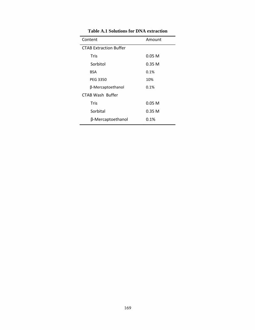
169
Table A.1 Solutions for DNA extraction
Content Amount
CTAB Extraction Buffer
Tris 0.05 M
Sorbitol 0.35 M
BSA 0.1%
PEG 3350 10%
β‐Mercaptoethanol 0.1%
CTAB Wash Buffer
Tris 0.05 M
Sorbital 0.35 M
β‐Mercaptoethanol 0.1%

170
APPENDIX B: ALLELE FREQUENCY FOR THE POLYMORPHIC MARKERS
Table B.1 The allele frequency test for polymorphic markers form software CERVUS Locus FreNull k N HObs HExp PIC HW OffName PtTX_2037 -0.0087 8 312 0.705 0.682 0.637 *** PtTX2037 PtTX_2080 0.018 5 274 0.697 0.706 0.658 *** PtTX2080 PtTX_2094 -0.1202 2 312 0.433 0.340 0.282 *** PtTX2094 PtTX_2146 -0.074 2 312 0.442 0.382 0.309 NS PtTX2146 PtTX_2158 -0.1223 2 312 0.439 0.343 0.284 *** PtTX2158 PtTX_2189 0.1402 3 274 0.453 0.568 0.493 *** PtTX2189 PtTX_3011 -0.0808 4 312 0.689 0.591 0.505 NS PtTX3011 PtTX_3013 -0.0685 6 312 0.846 0.738 0.695 *** PtTX3013 PtTX_3017 -0.144 2 95 0.505 0.380 0.306 NS PtTX3017 PtTX_3018 0.1705 5 312 0.372 0.483 0.456 *** PtTX3018 PtTX_3019 -0.1405 2 95 0.495 0.374 0.303 NS PtTX3019 PtTX_3021 -0.0765 2 312 0.529 0.454 0.351 NS PtTX3021 PtTX_3025 -0.0511 3 312 0.622 0.562 0.475 NS PtTX3025 PtTX_3029 -0.0509 7 312 0.801 0.715 0.673 *** PtTX3029 PtTX_3030 -0.0022 6 274 0.708 0.701 0.653 *** PtTX3030 PtTX_3034 -0.0354 7 312 0.769 0.717 0.680 *** PtTX3034 PtTX_3045 -0.0374 9 267 0.869 0.803 0.780 *** PtTX3045 PtTX_3049 -0.0484 3 133 0.707 0.621 0.550 *** PtTX3049 PtTX_3052 -0.0197 2 229 0.507 0.488 0.368 NS PtTX3052 PtTX_3055 0.014 5 312 0.583 0.595 0.531 NS PtTX3055 PtTX_3081 0.0137 3 312 0.628 0.610 0.541 *** PtTX3081 PtTX_3105 -0.1092 5 95 0.979 0.794 0.756 *** PtTX3105 PtTX_3107 -0.1501 6 218 0.633 0.514 0.489 *** PtTX3107 PtTX_3116 -0.0785 9 234 0.953 0.824 0.801 *** PtTX3116 PtTX_3117 0.0203 5 218 0.697 0.699 0.653 *** PtTX3117 PtTX_3118 -0.1231 3 175 0.469 0.384 0.347 * PtTX3118 PtTX_3120 -0.1254 2 312 0.449 0.349 0.287 *** PtTX3120 PtTX_4001 -0.2492 3 39 0.974 0.633 0.555 *** PtTX4001 PtTX_4003 -0.1489 3 93 0.559 0.440 0.391 NS PtTX4003 PtTX_4011 -0.1568 2 46 0.543 0.400 0.317 ND PtTX4011 PtTX_4030 -0.0688 9 312 0.913 0.802 0.773 *** PtTX4030 PtTX_4033 -0.0403 6 312 0.724 0.658 0.616 *** PtTX4033 PtTX_4056 -0.1279 2 57 0.456 0.355 0.290 ND PtTX4056
Notes: FreNull: Frequency of null allele; K: Number of alleles per locus; N: Number of observation; HOBs: Observed heterozygoisty; HExp: Expected heterozygosity; PIC: Polymorphic information content; HW: Significance test of Hardy-Weinberg equilibrium; OffName: the official name used for the SSR markers in collaborative data base.
For H-W: NS = not significant, * = significant at the 5% level, ** = significant at the 1% level, *** = significant at the 0.1% level, ND = not done. These significance levels include a Bonferroni correction.
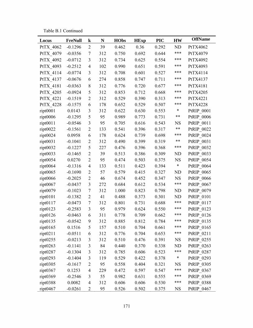
171
Table B.1 Continued
Locus FreNull k N HObs HExp PIC HW OffName
PtTX_4062 -0.1296 2 39 0.462 0.36 0.292 ND PtTX4062 PtTX_4079 -0.0356 7 312 0.750 0.692 0.644 *** PtTX4079 PtTX_4092 -0.0712 3 312 0.734 0.625 0.554 *** PtTX4092 PtTX_4093 -0.2512 4 102 0.990 0.651 0.591 *** PtTX4093 PtTX_4114 -0.0774 3 312 0.708 0.601 0.527 *** PtTX4114 PtTX_4137 -0.0676 6 274 0.858 0.747 0.711 *** PtTX4137 PtTX_4181 -0.0363 8 312 0.776 0.720 0.677 *** PtTX4181 PtTX_4205 -0.0924 5 312 0.853 0.712 0.668 *** PtTX4205 PtTX_4221 -0.1519 2 312 0.529 0.390 0.313 *** PtTX4221 PtTX_4228 -0.1575 6 178 0.652 0.529 0.507 *** PtTX4228 ript0001 0.0143 3 312 0.622 0.630 0.553 * PtRIP_0001 ript0006 -0.1295 5 95 0.989 0.773 0.731 ** PtRIP_0006 ript0011 -0.0546 3 95 0.705 0.616 0.543 NS PtRIP_0011 ript0022 -0.1561 2 133 0.541 0.396 0.317 ** PtRIP_0022 ript0024 0.0958 6 178 0.624 0.739 0.698 *** PtRIP_0024 ript0031 -0.1041 2 312 0.490 0.399 0.319 ** PtRIP_0031 ript0032 -0.1227 5 227 0.476 0.396 0.368 *** PtRIP_0032 ript0033 -0.1465 2 39 0.513 0.386 0.309 ND PtRIP_0033 ript0054 0.0270 2 95 0.474 0.503 0.375 NS PtRIP_0054 ript0064 -0.1316 4 133 0.511 0.423 0.394 * PtRIP_0064 ript0065 -0.1690 2 57 0.579 0.415 0.327 ND PtRIP_0065 ript0066 -0.2025 2 46 0.674 0.452 0.347 NS PtRIP_0066 ript0067 -0.0437 3 272 0.684 0.612 0.534 *** PtRIP_0067 ript0079 -0.1023 7 312 1.000 0.823 0.798 ND PtRIP_0079 ript0101 -0.1382 2 41 0.488 0.373 0.301 ND PtRIP_0101 ript0117 -0.0473 7 312 0.801 0.731 0.688 *** PtRIP_0117 ript0123 -0.2583 3 95 0.979 0.624 0.550 *** PtRIP_0123 ript0126 -0.0463 6 311 0.778 0.709 0.662 *** PtRIP_0126 ript0135 -0.0542 9 312 0.885 0.812 0.784 *** PtRIP_0135 ript0165 0.1516 5 157 0.510 0.704 0.661 *** PtRIP_0165 ript0211 -0.0511 6 312 0.776 0.704 0.653 *** PtRIP_0211 ript0255 -0.0213 3 312 0.510 0.476 0.391 NS PtRIP_0255 ript0263 -0.1141 3 84 0.440 0.370 0.338 ND PtRIP_0263 ript0287 -0.1304 3 312 0.785 0.606 0.523 *** PtRIP_0287 ript0293 -0.1404 3 119 0.529 0.422 0.378 * PtRIP_0293 ript0305 -0.1617 2 95 0.558 0.404 0.321 NS PtRIP_0305 ript0367 0.1253 4 229 0.472 0.597 0.547 *** PtRIP_0367 ript0369 -0.2546 3 55 0.982 0.631 0.555 *** PtRIP_0369 ript0388 0.0082 4 312 0.606 0.606 0.530 *** PtRIP_0388 ript0467 -0.0261 2 95 0.526 0.502 0.375 NS PtRIP_0467

172
Table B.1 Continued
Locus FreNull k N HObs HExp PIC HW OffName
ript0767 0.1565 3 312 0.462 0.615 0.533 *** PtRIP_0767 ript0647 -0.1377 3 117 0.521 0.419 0.376 * PtRIP_0647 ript0690 0.0042 5 256 0.711 0.711 0.659 *** PtRIP_0690 ript0791 -0.1347 4 312 0.49 0.374 0.306 *** PtRIP_0791 ript0792 -0.1303 4 124 0.508 0.422 0.394 * PtRIP_0792 ript0814 0.1184 5 178 0.472 0.595 0.558 NS PtRIP_0814 ript0852 -0.1296 2 312 0.462 0.356 0.292 *** PtRIP_0852 ript0947 -0.1204 3 312 0.462 0.381 0.348 *** PtRIP_0947 ript0968 -0.0693 6 312 0.913 0.798 0.768 *** PtRIP_0968 ript0984 -0.1243 3 175 0.469 0.381 0.340 * PtRIP_0984 ript1027 -0.0909 8 312 0.974 0.823 0.799 ND PtRIP_1027 ript1040 -0.0998 7 312 0.926 0.764 0.725 *** PtRIP_1040 ript1077 -0.1653 2 95 0.568 0.409 0.324 * PtRIP_1077 ript9058 -0.1127 3 312 0.580 0.468 0.409 *** PtRIP_9058 ript9104 -0.1382 2 41 0.488 0.373 0.301 ND PtRIP_9104 RPTest01 -0.1294 3 202 0.490 0.397 0.357 ** RPtest01 RPTest05 -0.1488 2 102 0.520 0.387 0.311 NS RPtest05 RPTest06 -0.1653 2 95 0.568 0.409 0.324 * RPtest06 RPTest09 -0.0658 4 312 0.554 0.474 0.417 NS RPtest09 RPTest15 -0.1284 3 229 0.480 0.386 0.342 *** RPtest15 sifg1003 -0.1244 2 312 0.446 0.347 0.286 *** PtSIFG1003 sifg1004 -0.1328 2 312 0.471 0.361 0.295 *** PtSIFG1004 sifg1008 -0.0986 2 312 0.365 0.299 0.254 * PtSIFG1008 sifg1018 0.0544 2 312 0.433 0.483 0.366 NS PtSIFG1018 sifg1024 -0.1322 3 312 0.484 0.380 0.327 *** PtSIFG1024 sifg1035 -0.1423 2 312 0.500 0.376 0.305 *** PtSIFG1035 sifg1036 0.0403 3 312 0.548 0.549 0.485 *** PtSIFG1036 sifg1052 -0.1333 2 55 0.473 0.364 0.296 ND PtSIFG1052 sifg1055 -0.0618 3 274 0.609 0.530 0.459 NS PtSIFG1055 sifg1058 -0.1307 4 272 0.500 0.408 0.373 *** PtSIFG1058 sifg1060 -0.0166 7 312 0.667 0.645 0.580 NS PtSIFG1060 sifg1061 -0.0318 7 312 0.728 0.677 0.632 *** PtSIFG1061 sifg1062 -0.2573 3 95 0.979 0.626 0.552 *** PtSIFG1062 sifg1064 0.0170 3 173 0.607 0.597 0.522 *** PtSIFG1064 sifg1069 -0.1066 2 41 0.390 0.318 0.265 ND PtSIFG1069 SsPp_cn524 -0.1514 2 55 0.527 0.392 0.313 ND SsPp_cn524 Ssrpt_ctg64 -0.1327 4 312 0.510 0.416 0.382 *** Ssrpt_ctg64 SsrPt_AW225917 -0.1545 2 41 0.537 0.397 0.316 ND SsrPt_AW225917SsrPt_AW981772 -0.1307 2 312 0.465 0.357 0.293 *** SsrPt_AW981772SsrPt_Ctg1525 -0.1060 3 312 0.484 0.391 0.335 ** SsrPt_Ctg1525

173
Table B.1 Continued
Locus FreNull k N HObs HExp PIC HW OffName
Ssrpt_Ctg2300 -0.0543 3 312 0.577 0.500 0.44 NS Ssrpt_Ctg2300 SSrPt_Ctg3021 -0.1452 4 41 1.000 0.757 0.700 ND SSrPt_Ctg3021 Ssrpt_Ctg3754 0.0517 3 117 0.530 0.578 0.486 NS Ssrpt_Ctg3754 Ssrpt_Ctg4698 -0.0162 4 312 0.548 0.477 0.43 NS Ssrpt_Ctg4698 SsrPt_Ctg7024 -0.1575 2 55 0.545 0.400 0.318 ND SsrPt_Ctg7024 SSrPt_Ctg7444 -0.1177 3 41 0.829 0.654 0.573 NS SSrPt_Ctg7444 SSrPt_Ctg7731 -0.1223 2 41 0.439 0.347 0.284 ND SSrPt_Ctg7731 SSrPt_Ctg865 -0.1545 2 41 0.537 0.397 0.316 ND SSrPt_Ctg865

174
VITA
Lisha Wu was born in Beijing, People’s Republic of China, in October, 1976. After
graduation from Hepingmen high school in Beijing in 1994, she enrolled in China Agricultual
University (CAU) and earned a Bachelor of Science degree in agronomy in July, 1998.
Because of her outstanding performances during the undergraduate study, she was accepted
as a master’s student in department of agronomy without entrance examination for graduate
school. Her research focused on establishing an efficient system for Agrobacterium
tumefaciens-mediated gene transformation for sweet potato under the instruction of Dr.
Qingchang Liu. Upon obtaining a master’s degree in June, 2001, she worked in the genetic
lab as research associate at the agronomy department. Her research was successful and her
results have a patent with IPC Number: A01H 4/00; C12N 1/20; C12N 5/04.
In 2003, she came to Louisiana State University (LSU) and started her doctoral
studies in the School of Renewable Natural Resources under the instruction of Dr. Michael
Stine and Dr. Thomas Dean. She worked on the molecular breeding for inproving early
height growth in longleaf pine, which is a project in cooperation with Southern Institute of
Forest Genetics (SIFG), USDA Forest Service. She also enrolled in a dual degree program for
experimental statistics at LSU, and received her 2nd master’s degree of applied statistics from
the Department of Experimental Statistics in May, 2008. Presently, she is a doctoral
candidate at the school of renewable natural resources.
Top Related