


![ICASE REPORT NO. ICASE - NASA · ICASE REPORT NO. 87-24 ICASE SINGULAR ... partial differential equation (e.g., ... Williams [19]. To describe the results in this classic paper, consider](https://static.fdocuments.net/doc/165x107/5af2ff227f8b9ac2469167ce/icase-report-no-icase-nasa-report-no-87-24-icase-singular-partial-differential.jpg)
Languages
Pages
Legal


NASA Contractor Report 172389
EASE REPORT NO. 84-24 I NASA-CR-172389I 198400214931
ICASEESTIMATION OF COEFFICIENTS AND BOUNDARYPARAMETERS IN HYPERBOLIC SYSTEMS
H. Thomas Banks
Katherine A. Murphy
Contract Nos. NASI-16394, NASI-17130
June 1984
INSTITUTE FOR COMPUTER APPLICATIONS IN SCIENCE AND ENGINEERINGNASA Langley Research Center, Hampton, Virginia 23665
Operated by the Universities Space Research Association
LIBIIARYCOPYNationalAeronautic=sand "' :'_ ! _. ]_84SpaceAdministration -
langley ResearchCenter LANGLEYRESEARCHCENTERLIBRARY,NASA
Hampton.Virginia 23665 HA.V,PTON_,VIRGINIA
https://ntrs.nasa.gov/search.jsp?R=19840021493 2018-11-09T19:05:29+00:00Z

5

ESTIMATION OF COEFFICIENTS AND BOUNDARY PARAMETERS
IN HYPERBOLIC SYSTEMS
H. Thomas Banks
Lefschetz Center for Dynamical Systems
Brown University
and
Southern Methodist University
Katherine A. Murphy
Southern Methodist University
ABSTRACT
We consider seml-discrete Galerkin approximation schemes in connection
with inverse problems for the estimation of spatially varying coefficients and
boundary condition parameters in second order hyperbolic systems typical of
those arising in I-D surface seismic problems. Spline based algorithms are
proposed for which theoretical convergence results along with a representative
sample of numerical findings are given.
Research supported in part by NSF Grant MCS-8205355, AFOSR Contract 81-0198,and ARO Contract AR0-DAAG-29-83-K0029. Parts of the research were carried out
while the first author was a visitor at the Institute for Computer
Applications in Science and Engineering (ICASE), NASA Langley Research Center,
Hampton, VA which is operated under NASA Contract Nos. NASI-16394 and NASI-17130.
i

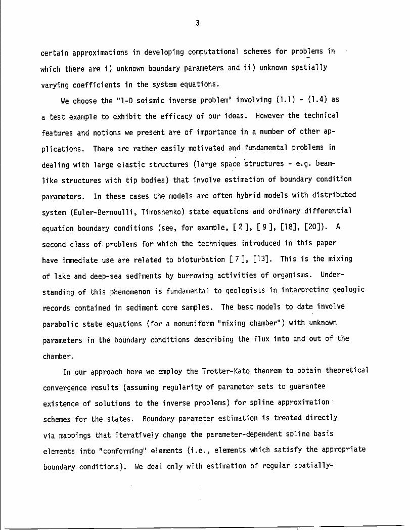
I. Introduction. In this paperwe considercomputationaltechniquesfor
the followingclass of inverseproblems: For the system
(I.I) p(X) a2v - a (E(x)av) t>O, O<x<l ,at2 @x @x
(I.2) ___(@vt,O) + klV(t,O)= s(t;k)
By(I.3) _t(t,l)+ k2-_-_(t,l)= 0
(I.4) v(O,x)= ¢(x) , vt(O,x)= ¢(x) ,
given observations{yij} for {v(ti,_)},choose,fromsome admissibleset,
"best"estimatesfor the parametersp, E, kl, k2, k. These problemsare
motivatedby certainversionsof the so-called"l-D SeismicInversionProblem"
(see,e.g. [l ], [8]). Roughlyspeaking,one has an elasticmedium (e.g.,
the earth)with densityp and elasticmodulus E. A perturbationof the system
(explosions,or vibratingloads from speciallydesignedtrucks)near
the surface(x=O)producesa sources for particledisturbancesv that travel
as elasticwaves, being partiallyreflecteddue to the inhomogeneousnature
of the medium. An importantbut difficultprobleminvolvesusing the observed
disturbancesat the surfaceor at points along a "bore hole" to determine
properties(representedby parametersin the system)of the medium. In the
highly idealizedl-D "surfaceseismic"problem,one assumesthat data are
collectedat the same point (x=O)where the originaldisturbanceor "source"
is located. In additionto this hypothesiswhich cannotbe true, other unreal-
istic specialassumptionsare made about the nature of the travelingand re-
flectedwaves. Althoughthe standardl-D formulationsare far from reality,

2
explorationseismologistshave developedtechniquesfor processingac%ualfield
data (performinga series of experimentsand "stacking"the data) so that the
l-D problemsare generallyacceptedas usefuland worthy subjectsof investi-
gation. Consequently,numerouspapers (forsome interestingreferences,see
the bibliographiesof [l ], [8 ]) on the l-D problemscan be found in the research
literature.
In many formulationsof the seismicinverseproblem,the medium is assumed
to be the half-linex>O (withx=O the surface)while in others (especially
some of those dealingwith computationalschemes)one finds the assumptionof an
artificialfiniteboundary (sayat x=l) at which no downgoingwaves are reflected
(an "absorbing"boundary). While there are severalways to approximatesuch a
conditionin 2 or 3 dimensionalproblems(see [12], [21]),for the l-D formulation
this conditionis embodiedin a simple boundaryconditionof the form (I.3);
here k2 : _ E(1)/p(1) and one can view this boundaryconditionas resulting
from factoringthe wave equation (l.l)at x=l and imposingthe conditionof
"no upgoingwaves" at x= I.
Equation(l.l) is a I'D versionof the equationsfor an isotropicelastic
mediumwhile (I.2) representsan "elastic"boundaryconditionat the surface
x= 0 (kI representsan elasticmodulusfor the restoringforce producedby the
medium).
As is the case in many inverseor "identification"problems,the problems
describedabove tend to be ill-posed(includinga computationallyundesirable
instability)unlesscarefulrestrictionsare imposedon the admissibleparameter
class (for some discussionsof these aspects,see [l ], [lO]). We shall not
focus on this aspecthere. Rather,the purposeof our presentationin this
paper is to demonstratethe feasibilityof a certaintheoreticalapproachand
certainapproximationsin developingcomputationalschemesfor problemsin
which there are i) unknownboundaryparametersand ii) unknownspatially
varyingcoefficientsin the systemequations.
We choose the "l-D seismicinverseproblem"involving(l.l)- (I.4) as
a test exampleto exhibitthe efficacyof our ideas. Howeverthe technical
featuresand notionswe presentare of importancein a number of other ap-
plications. There are rather easilymotivatedand fundamentalproblemsin
dealingwith large elasticstructures(largespacestructures- e.g. beam-
like structureswith tip bodies)that involveestimationof boundarycondition
parameters. In these cases the modelsare often hybridmodels with distributed
system (Euler-Bernoulli,Timoshenko)state equationsand ordinarydifferential
equation boundaryconditions(see,for example,[2 ], [9 ], [18], [20]). A
secondclass of problemsfor which the techniquesintroducedin this paper
have immediateuse are relatedto bioturbation[7], [13]. This is the mixing
of lake and deep-seasedimentsby burrowingactivitiesof organisms. Under-
standingof this phenomenonis fundamentalto geologistsin interpretinggeologic
recordscontainedin sedimentcore samples. The best models to date involve
parabolicstate equations(fora nonuniform"mixingchamber")with unknown
parametersin the boundaryconditionsdescribingthe flux into and out of the
chamber.
In our approachherewe employthe Trotter-Katotheoremto obtain theoretical
convergenceresults(assumingregularityof parametersets to guarantee
existenceof solutionsto the inverseproblems)for spline approximation
schemesfor the states. Boundaryparameterestimationis treateddirectly
via mappingsthat iterativelychange the parameter-dependentsplinebasis
elementsinto "conforming"elements(i.e.,elementswhich satisfythe appropriate
boundaryconditions). We deal onlywith estimationof regularspatially-

4
varyingcoefficientsin (I,I);where again splinesare used for parameters
in a secondaryapproximation. Estimationof discontinuouscoefficients
(includinglocationof the discontinuities)in problemssuch as those that
are the focus of our attentionin this paper can be effectivelytreated
theoreticallyand numericallyin a frameworksimilarto that here using,
for example,tau-Legendrestate approximationschemes[4 ].
We turn then to the estimationproblemfor{l.l)-(l.4). It is theoretically
and numericallyadvantageousto deal with homogeneousboundaryconditionsby
transformingthe problemso that the source term s in (I.2) appearsin the
initialdata and in a term in the state equation. We make the transformation
u = v + G where {here "." representsdifferentiationwith respectto t)
and obtainthe system
ql(x_@2u - B x Bu- -- (q2()_-_)+ F(t,x;q)JBt'_ @x
Ux(t,O)+ q3u(t,O)= 0
(1.5)
ut(t,l)+ q4Ux(t,l)= 0
u(O,x): _(x;q) , ut(O,x) : _(x;q).
Here the forcingfunctionF is given by
_ _ {q2(X)(q3-3_--44)(Bx2-2x)_(t;k)}BX

5
where here and throughoutwe adopt the notationq : (ql'q2' q3' q4"_) with
ql --p' q2 - E, q3 = kl' and q4 = k2" The transformedinitialconditionshave
the form
We assume henceforththat we have observationsYi = il' ""_ im) '
i=l, 2, ..., n, correspondingto w(ti;q)= (u(ti,xl),.-.,u(ti,Xm))where ^
u is the solutionof (I.5). For a criterionin determininga best estimateq
of the parameterswe use a least-squaresfunction
n _ 2
(I.6) J(q)= i__SllYi- w(ti;q)l
which we seek to minimizeas q rangesover some admissibleparameterset Q.
We remark that in the event our observationsni = ( il' ""' im) are for the
originalsystem (l.l)-(l.4),we may apply directlythe theoryand techniques
of this paper by consideringin place of (I.6)the criterion
n
(1.7) J(q) = Z Ini + G(ti;q)- w(ti;q)l2i=l
where G(ti;q)_ (G(ti,xl;q),...,G(ti,Xmlq))•
We make some standingassumptionsto facilitateconsiderationof our
problemin subsequentdiscussions. We shall searchfor q in a set
Q:C(O,I) x Hl(o,l)x R x R x Rk (we shall sometimeswriteQ as Ql x Q2 ×
Q3 × Q4 × Q5)" we furtherassume that Q is compactin the C x Hl x R2+k
topology,and that there exist positiveconstants

qi ' qi ' i=l, 2, 3, 4 such thatu
qi _qi {X) _qi for qieQi ' i=l, 2,
q3 < "q3 < q3 for q3e Q3 ' and
q4 _q4 _q4 for q4eQ4 "
Finally,we assume@eHl(o,l) , _eHO(o,l) , and s(.;k)eH3(O,T) for each
eQs, where tie[O,T], T<_, and that k . s(.;k) is a continuousmappingfrom
Q5 to H3(O,T)"
We turn next to the theoreticalfoundationsof the approximationschemes
we proposeto use in solvingour inverseproblemof minimizingJ over Q,
subjectto (I.5).

2. AbstractFormulation.
The object in this sectionis to lay the theoreticalfoundationfor the
problem. First,we shallwrite our partialdifferentialequationas an abstract
ordinarydifferentialequationin a Hilbertspace,then determinea set of
approximatingordinarydifferentialequations. Each of these abstractequations
will have an associatedidentificationproblem;the originalwill be referred
to as (ID),the Nth approximatingproblemwill be referredto as (IDN). We
shall use the theoryof semigroupsto obtain existenceand uniquenessof
solutionsto the differentialequations. We can then fit our probleminto the
theoreticalframeworkdevelopedin [ 5 ], and deducethat, under conditions
statedthere (reiteratedbelow for clarity),one can solve (IDN) for each N,
and these parameterestimatesthus obtainedwill "lead to" a solutionof (ID).
The equation(I.5) can be rewrittenas a first order system,motivating
the use of a product(V(q)x L2(q)) of two spacesto be our Hilbertspace X(q).
DefineV(q) to be Hl(o,l)with inner productdefinedby <v,W>v(q)=
_l q2DvDwdx- q2(O)q3v(O)w(O). (D denotesthe spatialdifferentiationoperator
) It can be readilyshown that for any q_Q V(q) is a Hilbertspace,and_X "
moreover,the assumptionsmade about Q imply that the V(q) norm is uniformly
equivalentto the Hl norm as q ranges over Q. Let VB(q) containthose elements
of V(q) which satisfythe elasticboundarycondition,i.e., VB(q) =
{veV(q)nH2(O,l)IDv(O)+ q3v(O)= 0}.
We define L2(q) to be HO(o,l)with inner productgiven by <v,W>o,q =
_l qlVWdx , and note for q_Q, L2(q) a space normthat each is Hilbert and its
is uniformlyequivalentto the standardH0 norm as q rangesover Q.
As describedearlier,we take X(q) = V(q) x L2(q) with inner product
given by <x,y>q = <Xl,Yl>V(q)+ <x2,Y2>o,q(wherex = (Xl,X2)Tand y = (yl,Y2)T).
It is clear from our remarksabove that for q_Q, X(q) is a Hilbertspace, and the

8
X norm is uniformlyequivalentto the HI× H0 norm as q rangesover Q. We can
formallywrite (I.5) as an abstractequationin ×(q):
z(t) : A(q)z(t)+ G(t;q)
(2.1)
z(O) : ZO(q)
where we have identifiedz(t)e X(q) with . The boundaryconditions
\ut(t, )
are incorporatedinto the domainof A(q) by definingdomA(q)= {(u)e VB(q) x
Hl(o,l)Iv(1)+ q4Du(1)= 0}, and A is the unboundedlinearoperatorgiven by
A(q) =
• (I/ql)D(q2D) 0
The functionG and the initialconditionare given by
and ZO(q) =G(t;q) = F(t,-;q) _(.;q)
It can be shown that for each qe Q, A(q) is the infinitesimalgeneratorof
a Co-semigroup,T(t;q) on X(q), so that we have the existenceof mild solutions
to {2.1),given by
t
(2.2) z(t;q)= T(t;q)zo(q)+ f T(t-s;q)G(s;q)ds0
with z(-;q){C(O,T;X(q)).In this context,the inverseproblemcan be stated as:
^ ^ ^n
(ID) Given observationsy = {Yi}i=l, minimizeJ(z(.;q),y)over qeQ
subjectto z(.;q)satisfying(2.2).

Here, J(q) _ J(z(.;q),y) : 1_llYi.: - {(ti,q)l 2 where _(ti,q) :
(zl(ti,xl;q) , ..., zl(ti,Xm;q) ) and zI denotes the first component of z.
To prove that for each q, A(q) generates a Co-semigroup, one can use the
Lumer-Phillips Theorem ([15], p.16). To employ this theorem, one must show the
operator is dissipative, densely defined, and satisfies a certain range statement.
To demonstrate the dissipativity of A(q), we take f{ domA(q), q e Q, and compute
(with an integration by parts)
<A(q)f,f>q=
(I/ql)D(q2Dfl) f2
: <f2,fl>V(q)+ <(llql)D(q2Dfl),f2>O,q
l l
:/oq2DflDf2dx-q2(°)q3fl(°)f2(°)+ D(q2Dfl)f2
: _ q2(O)q3fl(O)f2(O)- q2(O)Dfl(O)f2(O)+ q2(1)Dfl(1)f2(1)
= - q2(1)q4(Dfl(1))2 <_0 .
ByrelatingdomA(q)to other subsets (see[l_.Fo,rdetails)which are known to
be dense in HIxH_ one can easilyargue that for each q eQ, domA(q)is dense
= X(q) for some _>0, by demon-canin X(q). One also argue that R(_-A(q))
stratingthat given f2 _X(q)' there exists edomA(q) such that
u_v) fl);(I/ql)D(q2Du)+ _v f2
This is equivalent to solving the following two point boundary value problem:

lO
- (I/ql)D(q2Du)+ _2u : _fl + f2
Du(O)+ q3u(O) = 0
_u(1) + q4Du(1)= fl(1)
for ue H2_O,l),and settingv(x) = _u(x) - fl(x).
If we let y = u - (I/q4)x2(x-l)fl(1)the above problemis transformed
to an equivalentone with homogeneousboundaryconditions:
(_i/ql)D(q2DY)+ _2y = F
Dy(O) + q3_(O) = 0
q4Dy(1)+ _y(1) = 0
where F_ L2(q). One can then use the theoryof self-adjointoperators(again
see[l_)to argue that a solutionexistsfor any F_ L2(q).
We now turn to the approximationof our equation (2.1). We shall obtain
a solutionzN to an approximatingequation (to be discussedin detail below)
in a finitedimensionalsubspaceof X(q), denotedxN(q). Specifically,let
S3(AN) representthe standardsubspaceof C2 cubic splinescorrespondingto
the partition_N =£xi_ , xi = i/N (seepp. 78-81 of [16]);then,=0
given q e Q, we take xN(q) to be that subspaceof s3(AN)x $3(_N) whose elements
satisfythe boundaryconditionscorrespondingto q (i.e.,XN(q)C domA(q) ).
Let B_ j = -l ,N+l,.be the B-splinebasis elementsfor $3(_N) Thenj ' _,oo •
xN(.q)is the (2N+ 3)-dimensionalsubspacespannedby the followingset of basis
functions:

II
l _ I- 4q3 ),_= , ,;= ,
o o /
13_: , • • - , 6_i : ,0
(B -I1 I 1B_ : _N : N :' N+I ' 8N+2 '
3Nq4 3Nq4 BNTB_ 0 T N
(-II 3Nq4'B I)(-II'3N 4'B I1N N6N+3 = , , 8N+4 : ,
N BNBN+l N-l
(0) (0)N = N_5 ' " " " ' 62N+I : '
N B_BN-2
N N62N+2 : , 62N+3 = .
Let pN(q):X(q).xN(q)denotethe orthogonalprojectionof X(q) onto
xN(q), i.e., given feX(q), pN(q)fis that elementin xN(q) which satisfies
IpN(q)f-f]q _ [g- fiq for all g e xN(q). For each qeQ, we definean operator

12
AN(q)onX(q) givenby AN(q)= pN(q)A(q)pNcq),and thentheapproximating
equationto (2.1)is writtenas:
_N(t) : AN(q)zN(t)+ pN(q)G{t;q)(2.3)
zN(o) : pN(q)zo(q)
where zN(t)e xN(q). Using the fact thatA(q) is closed,pN(q) is bounded,
and the _osed Graph Theorem,one finds thatAN(q) is bounded. The operator
AN(q) inheritsthe dissipativityof A(q), and thereforeit followsthat for
each qs Q, AN(q) is the infinitesimalgeneratorof a Co-semigroup of contractions
TN(t;q)on X(q). It is readilyseen that TN(t;q)leavesxN(q) invariant. Thus,
for each qsQ and each N=l,2, ...,there existsa uniquemild solution
zN(';q)e C(O,T;XN(q))of (2.3),which can be expressedas
(2.4) zN(t;q): TN(t;q)pN(q)Zo(q.) + _otTN(t_s;q)pN(q)G(s;q)ds.
The associatedapproximateidentificationproblemis given by
(IDN) Given observationsy = _ _i=l' minimizeJ(zN(.;q),y)over qeQsubjectto zN(.;q)satisfying(2.4).
Here, jN(q) _ j(zN(.;q),_)= i_l.i_i _ {N(ti,q)12where {N(ti,q)=
(z_(ti,xl;q),...,z_(ti,Xm;q))and z_ denotesthe first componentof zN.
Since xN(q) is finite dimensional,(2.3)is in fact a systemof 2N+3
ordinarydifferentialequations,which can be solvedusing standardnumerical
packages. Similarly,there are numericalpackagesavailableto solve (IDN),
providedsolutionsexist and we have some computationallyfeasiblerepresentation
for ql and q2" A detaileddescriptionof our numericalimplementation,
includinga discussionof possiblerepresentationsof ql and q2' will be deferred
13
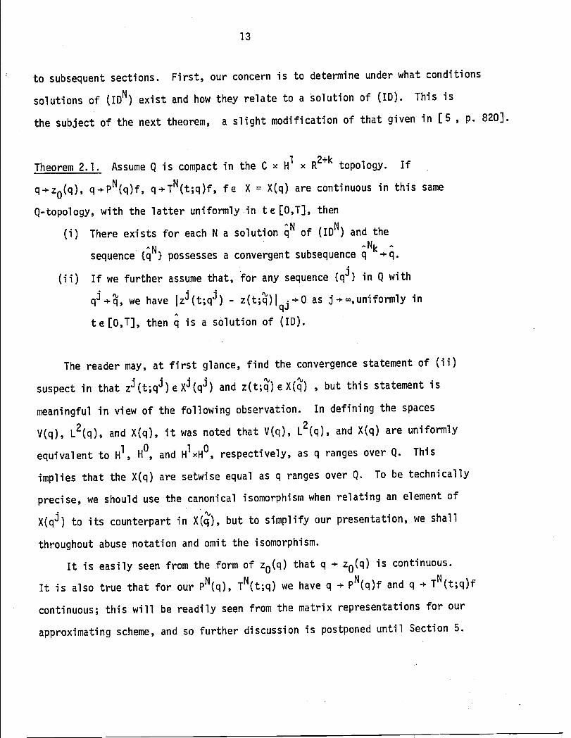
to subsequentsections. First,our concernis to determineunderwhat conditions
solutionsof (IDN) exist and how they relateto a Solutionof (ID). This is
the subjectof the next theorem, a slightmodificationof that given in [5 , p. 820].
• R2+kTheorem2.1 Assume Q is compactin the C x Hl x topology. If
q.zo(q), q.pN(q)f, q.TN(t;q)f, fe X = X(q) are continuousin this same
Q-topology,with the latteruniformlyin te [O,T],then
(i) There exists for each N a solutionGN of (IDN) and the1 ^Nk ^
sequence{qN} possessesa convergentsubsequenceq -.q.
(ii) If we furtherassume that,for any sequence{qJ} in Q with
zj _ lqjqJ.q, we have [ (t;qj) - z(t;q) .0 as j._,uniformly in^
te[O,T], then q is a solutionof (ID).
The readermay, at first glance,find the convergencestatementof (ii)
suspectin that zJ(t;qj)e XJ(qj) and z(t;_)eX(_) , but this statementis
meaningfulin view of the followingobservation. In definingthe spaces
V(q), L2(q), and X(q), it was noted that V(q), L2(q),and X(q) are uniformly
equivalentto Hl, HO, and HI×HO, respectively,as q rangesover Q. This
impliesthat the X(q) are setwiseequal as q rangesover Q. To be technically
precise,we shoulduse the canonicalisomorphismwhen relatingan elementof
X(qj) to its counterpartin X(q), but to simplifyour presentation,we shall
throughoutabuse notationand omit the isomorphism.
It is easily seen from the form of ZO(q) that q . ZO(q) is continuous.
It is also true that for our pN(q),TN(t;q)we have q . pN(q)f and q . TN(t;q)f
continuous;thiswill be readilyseen from the matrix representationsfor our
approximatingscheme,and so furtherdiscussionis postponeduntil Section5.

14
The next theoremgives sufficientconditionsfor the hypothesis..of(ii)from Theorem2.1 to hold.
Theorem2.2 Let qN, _ be arbitraryin Q such that qN . q as N . _ (recall
convergenceis in the C x Hlx R2+ktopology). Supposethat the projections
pN(q) are such that I(pN(qN)-l)fJ N.O as N . _ for all feX(_), thatf_ X(_) JTN(t;qN)f-
T(t; ) lqN+Oas uniformlyin andimplies
that Jzo(qN) - Zo(_)j N . 0 as N . _. Then the mild solutionszN(t;qN)ofq
(2.3)convergeto the mild solutionz(t;_) of (2.1) uniformlyin te[O,T].
The proof of this theorem,which is based on a standard"variation-of-
constants"representationfor solutionsz and zN in terms of the semigroups
T and TN, essentiallyfollowsimmediatelyfrom Theorem3.1 of [5, p. 823].
One only needs to verify that our spaces,operators,etc. satisfythe conditions
requiredin [ 5 ].
Zo(qN) qN._It is clear from the continuity of q . ZO(q) that I -Zo!_) I .0 as q.:qN
It remains only to show the convergence of the projections and the semigroups.
The main result of the next section is the convergence of the semigroups; the
convergence of the projections is obtained as an intermediate proposition.
In summary then, at the end of the next section, we will be able to deduce
zN(t;q N) qNfrom Theorem 2.2 that converges to z(t;_) whenever . q, and hence
by Theorem 2.1 we are assured that the sequence of iterates {GN} we obtain
(iD N ^by solving ), has a subsequence which converges to a solution, q, of (ID).

15
3. ConvergenceArquments.
This sectionwill be devotedto establishingthe result: For each convergent
sequenceqN . q in Q, and for any feX(_), ITN{t;qN)f- T(t;_)flqN. 0 as
N . _, uniformlyin t_ [O,T]. As explainedin the previoussection,this
convergenceresult is crucialin arguingthat zN(t;qN) . z(t;_)whenever
qN . q, which in turn is necessaryto ensure that our candidate(.thelimit of
our approximatingsubsequence)is indeeda solutionto our inverseproblem.
We shall first prove a slightlydifferentform of convergenceof the semi-
groupsusing the followingversionof the Trotter-KatoTheorem[3 ].
Theorem3.1. Let (B,{.{)and (BN,I.IN), N : I, 2, ...,be Banach spacesand
let fIN.•B.B N be boundedlinearoperators. Furtherassumethat T(t) and TN(t)
are Co-semigroupson B and BN with infinitesimalgeneratorsA and _N, respectively.
If
(i) lim { Nf{N= Ifl for all feB,N_
(ii) there exist constantsM, m independentof N such that
ITN(t)IN_Me mt, for t _0,
(iii) there exists a set DCB, PC dom(A),with (_o-A)D= B for
some _0>0' such that for all feP we have
I_NRNf- RNAf{N. 0 as N . _ ,
then ITN(t)_Nf-RNT(t)fIN. 0 as N . _, for all feB, uniformlyin t on compact
intervalsin [0,_).
It will be a standingassumptionthroughoutthis sectionthat qN . q
R2+k X _in Q with this convergencein the C x Hl x topology. Let B = (q) with
norm denotedby {'l_,BN = X(qN) with norm l'l for N = l, 2, ...,A = A(q)q qN

16
With correspondingsemigroupT(t) : T(t;_),and _N = AN(qN) = pN(qN)A(qN)pN(qN)
with correspondingsemigroupTN(t) = TN_t;qN) {as describedin Section2). For
each N, fIN:X(_) . X(qN) will be a boundedlinearoperatorwhich will map elements
of domA(_)into elementsof domA(qN). Define
= -cx/
The functions gN are defined so that as N . _, gN(x) . I, and DJ(gN(x)).O
for any positive integer j, where in each case the convergence is uniform
in x_[O,l].
A simple computation demonstrates that if fe dom A(_), then fiNfe dom A(qN).
For each N, fin is a bounded linear operator from X(_) to x(qN), but moreover,
the set of operators {IIN} is uniformly bounded. This statement can be proved
using the assumptions on Q and the properties of gN mentioned above. Similar
comments apply to the proof of our first proposition.
Proposition3.1. For any feX(_), IfiNf-flaN . 0 as N . _.
In order to argue the convergence of the infinitesimal generators, we
shall need error estimates for the spline approximations and their derivatives.
These will be variations of estimates such as those found in [19], modified
to take into account our q-dependent norm, and the presence of the operatorfiN.

17
The followingnotationwill be used throughoutthis section. Given a
vectorfunctionf, we Shall use fi or (f)ito denote the ith componentof f.
Given the scalarfunctionh, INh will denotethe standardcubic spline
interpolantof h (thus INh e S3(AN)). For a vector functionf = f2 ' INf
will be the vectorwhose componentsare the splineinterpolantsof the
INfl )componentsof f, i.e., INf = and INf e S3(AN) x S3(AN). The
INf2
interpolantof f which satisfiesthe bounda_ conditionscorrespondingto
q will be writtenas I_(q)f. While INf interpolatesfl and f2 at the values
_i/N)_=O and the derivativesof fl and f2 at O and l, I_(q)fwill interpolate
fl and f2 at the values_/_=0, andwill additionallysatisfy
[D(l_(q)f)i](O) + q_{I_(q)f)i](O)= O, or equivalently,
[D(l_(q)f)i](O) =- q3fi(O) for i = l, 2,and
[{l_(q)f)2](l) + q4[D(l_(q)f)l](1)= O, or equivalently,
[D(I_(q)f)l](l) =_ (I/q4)f2(1).
We note that if f satisfiesthe boundaryconditionsinvolvingq, then
IN(q)f : INf.
The first estimates involve cubic interpolants for scalar functions.
Lamina3.1. If h e H2, then
ID2(h-INh)lo. 0 as N . _ ,
< N-IID2(h_INh){o_<N"IID2h{oID(h-INh)lo_
{h - INhlo< N-21D2(h-INh)lo<__ N-21D2h{o
The convergencestatementof this lemma followsimmediatelyfrom the
densityof H3 in H2, the estimatesof Theorem6.9 of [19], and the first

18
integralrelation(4.15)of [19]. The estimatesfollowfrom (4.24)and (4.25),
respectively,of [19] and the first integralrelation.
One can use the resultsof Lemma 3.1 and the equivalenceofthe X(q)
and Hl x H0 norms to derive similarstatementsfor the interpolantsin the
X(q) norm.
Lemma 3.2. If f e H2xH 2 and q e QCCxHI×R 2+k, then
IINf-flq_< KiN-l!ID2(fl- INfl)l2 + ID2(f2-INf2)l_)I/2
<_K1N-I(ID2fll+ ID2f21 )1/2
IO(INf-f)lq< K2(lo2(fI - INfl)l2 + ID2(f2-INf2)l_)I/2
where Kl, K2 are constantswhich are independentof f, q, and N.
Again, due to the equivalenceof norms, the Schmidtinequalityof [l_, Thm. 1.5]
can be modifiedand used component-wiseto give a Schmidttype inequalityin
the X(q) norm.
Lemma3.3. If feS3(A N) x S3(AN) and q eQ, then IDflq < K3Nlflq , where
K3 is a constant independent of f, N, and q.
The precedingestimatescan be used to establishconvergenceproperties
for the canonicalprojectionspN(qN)where qN . _ in Q.
Proposition3.2. If fe X(_), then
IpN(qN)f- flqN . 0 as N +
Proof. Firsz considerf_domA(_)N(H2×H2). For such f, RNfedomA(qN)n(H2xH 2)
19
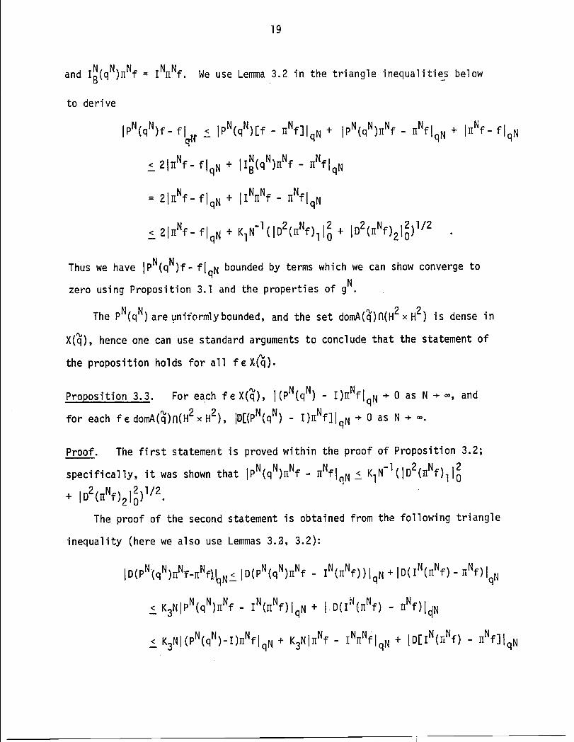
and l_(qN)_Nf = IN_Nf. Weuse Lemma3.2 in the triangle inequalities below
to deri ve
IpN(qN) f-fl_ _ IpN(qN)[ f - _Nf]lqN + IpN(qN)_Nf - _NflqN + {_Nf_ flqN
2{_Nf-f{qN + ll_ (qN)_Nf - _NflqN
: 21_Nf- flqN + {IN_Nf - RNflqN
21RNf-flqN + KIN-I(ID2(RNf)I{_ + {D2(RNf)21_)I/2 "
Thus we have IpN(qN)f - flqN bounded by terms which we can show converge toN
zero using Proposition 3.1 and the properties of g
The pN(qN) areuniformlybounded, and the set domA(_)n(H2xH 2) is dense in
X(_), hence one can use standard arguments to conclude that the statement of
the proposition holds for all feX_).
Proposition 3.3. For each feX(_), l(pN(q N) - l)_NflqN . 0 as N +-, and
for each fedomA(_)n(H2xH2), ID[(pN(qN) - l)RNf]{qN . 0 as N .-.
Proof. The first statement is proved within the proof of Proposition 3.2;
specifically, it was shown that IpN(qN)RNf - RNf{qN £ KIN-I(ID2(RNf)II _
+ ID2( Nf)21 )I/2.The proof of the second statement is obtained from the following triangle
inequality (here we also use Lemmas3.8, 3.2):
{D(pN(qN)RNT-RNf_N_{D(pN(qN)_Nf - IN(_Nf))lq N+ID(IN(RNf)-RNf)IqN
K3N{pN(qN)_Nf - IN(RNf)IqN + I D(IN(_Nf) - nNf)l_N
K3Nl(pN(qN)-l)_NflqN + K3NIRNf - INRNflq N + ID[IN(RNf) - _Nf]IqN

20
<__2K3NIINIINf-.IINflqN +.ID[IN_Nf-IINf]lqN
< (2KIK3+ K2)(ID2[oINf)I- IN(_Nf)l]l_+ JD2[(RNf)2-IN(HNf)2]il_)I/2
Thusthe conclusionID[(pN(qN) I)IINf]lqN. 0 as N . _ followsfromthe
observationthatfor i = 1,2
ID2[IN(IINf)i- (IINf)i]l0 < ID2[IN((IINf)i-fi)]lO
+ ID2[INfi - fi]{O + ID2[fi- (IINf)i]l0
<__21D2[(IINf)i - fi]Io+ {D2[INfi - fi]Io ,
with the latterterms approachingzero becauseof the propertiesof gN
and Lemma 3.1, respectively.
In later arguments,it will be helpfulto have bounds (in the Hl and H0
norms) on one componentof an elementof X in terms of a bound (in the X(q) norm)
on the entireelement. Thus, we considerfor faX(q), Ifl_= Ifll_(q) +
If21_,q which is equivalentto IDfiI_+ Ifll_+ {f21_ , so that there exist
2andI_I_<k21fI_Similarly,constantskIand k2 such that IDfII__ kIIflq _ •2
IDfl_= IDfiI_(q)+ {Df210,qwhich is equivalentto ID2fl{_+ !Dfll_+ {Df21_
so we infer the existenceof constantsk3 and k4 such that ID2fII__ k31Dfi_
and{Dr21__k4IDfI_.Forfuturereference,we combineandlabeltheseobservationsas
IDfII_ < kIIf{2- q
2
(3.1) ID2flI__ k31Dflq
{f2J2<k21fl+k41Dfll-
It is now possibleto state and prove the followingconvergencetheorem.

21
Theor_ 3.2, SupposeqN . q in Q (convergenceis in the Cx H1× R2+k topology).
Then
ITN(t;qN)_Nf - _NT_t;_)flqN . 0 as N . _ ,
for all feX(_), unifo_ly in t on c_pact intervals in [0,_).
Proof. The result is an i_ediate consequence of Theorem 3.1, once the
hypotheses of that theorem have been shown to hold. Part (i) follows from
Proposition 3.1, while pant (ii) holds since TN(t;q) and T(t;q) are
contraction semigroups for each N and qeQ. It remains only to veri_ (iii),
for which we take D to be the set do_(_)N(H2xH2). Let feD. Then
IAN(qN)_Nf - _Na(_)flq N = Ipm(qN)m(qN)pN(qN)_Nf- _Na(_)flq N
IpN(qN)[A(qN)pN(qN)_Nf - _NA(_)f]IqN + IpN(qN)RNA(_)f - _NA(_)flqN
_ IA(qN)pN(qN)_Nf-_NA(_)flqN+I_N(qN)-I)RNA(_)f[qN
_ el(N) + c2(N).
It followsdirectlyfrom Proposition3.3 that c2(N). 0 as N . _ . We must
work harder to establishthat _l(N). O. We begin by breakingthe norm into
its two componentsand treat each separately. Thus
[_I(N)]2 = (pN(qN)_Nf) _ _N
i/q )o(qo) qN
: l(pN(qN)_Nf)2 - gNf21_(qN)
N_ NI_ _ 2+ I(I/q_)D[q_D(pN(qN)RNf)I ] - Cq4/q4)g ( /ql)D[q2Dfl]iO,qN
22
- [a:l(N)]2+ [a2_N)]2 ..
We firstobservethat
N tb
al(N) < [(pN(qN)_Nf)2-(q_/_4)gNf2lv(qN)+ ][(q4/q4)- l]gNf2]V(qN)
= {(pN(qN)IINf)2-(IINf)2]V(qN)+ ]((q_/_4)-l)gNf2[V(qN) •
It is more convenient,and due to the equivalenceof the norms, it is sufficient,
to establishthe convergencein the Hl norm. This can easily be done for the
first term by invokingProposition3.3 and the inequalities(3.1). An argument
can be made for the second term based on the propertiesof the gN and the
qNconvergence . q.
We turn now to the estimationof a2(N). Using the equivalenceof the
L2(qN) and H0 norms,and the inequalities(3.1),we establishthe following
chain of inequalities:
a2(N) = l_]__D[q_ D(pN(qN)_Nf)I]- "q4Cq_ gN) _--qlD(q2Dfl)IO'qrl
which is equivalentto
+-- - L-- _-- -L-- _-- 01 q4 ql q4 ql
qN L qN DqN _, N
+ _ Dq2(q4 N,<_lq_2D2(pN(qN)IINf)l_ _lq2(__44gN)D2flq4lO l D(pN(qN)IINf)I-_'--ql7gq4jDfl[0

23
__ (q._4)gNDZfl iO +
- ql qlq4
Dq_ .< =ID[(pNcqNI-IIRNf]IqN+i_-_ioJD(CpN(qN)-ll_Nflli=+ql
q2,q4, N Dq2
'q_ D2(IINf)l-_--t_--)gqlq4 D2fliO+i_ D(IINf)l'-_-iq4(_ gN)Dfll0
We thus see that a2(N) can be boundedby four terms which go to zero as N._;
the convergenceof the first two terms is the resultof Proposition3.3 and
the convergenceof qN to q, while the convergenceof the second two can beN N
arguedusing the propertiesof g and q .q.
We can use this theorem,the convergencepropertiesof the operatorsRN
(Proposition3.1), and the semigroup properties of TN and T, to establishthe
final resultwe need, as a corollary.
Corollary3.1. SupposeqN._. Then
ITN(t;qN)f T( _- t;q)flqN. 0 as N .
X _for all f_ (q), uniformlyin t on compactintervalsin [0,_)

24
We can now invokethe results(seeTheorems2.1 and 2.2) stated in Section2
to concludethat q (obtainedthere as the limit of an approximatingsubsequence,A
{qNk})is a solutionto the identificationproblem.

25
4. ParameterApproximation.
In Section2,_we pose the problemof minimiz_ingjN(q) over Q. The
argumentsunderlyingTheorem2.1 yield that (undercertainassumptions)
each Nth (approximate)problemhas a solutionGN, and for any convergent
{qNk}, G ^ ^subsequence with Nk . q, we have q is a solutionof the original
identificationproblem. Recall,however,that ql and q2 are functional
coefficients,and hence each of the approximateoptimizationproblemsis in
fact infinitedimensionalin nature. In this section,we discusssome
methodsfor approximatingthese infinitedimensionaloptimizationproblems
by finitedimensionalones, thus providingnumericallytractableproblems.
This, of course,resultsin a second,or parameter,approximationthat must
be considered.
In Section5, we shall presentthe resultsof severalnumericaltest
examples. To reduce ill-posedness(see the commentsin Sectionl) we set
ql = p _ l and search for q2 _ E, q3' q4' _' with q2 the only functional
unknown. We thereforerestrictour theoreticaldiscussionshere to this
case. (Wenotehoweverthat in principle,our methodsand ideas can be applied
to the estimationof both p and E.)
An approachthat one might takewould be to assumeana priori parameter-
izationfor q2" Thus the estimationof the unknownfunctionbecomesthe esti-
mation of a set of unknownConstantsappearingin the parameterization.The
convergencetheorydevelopedthus far is directlyapplicableto thismethod.
However,it would onlyyield resultsfor best approximates(throughthe cri-
terionon state observations)to q2 withinthefixe_____dd_prioriparameterization
class. Little can be said about convergenceto a "best fit parameter"q2 from
the originalparameterset Q.
26
An alternateapproach,which does not require,qualitative(e.g_,shape)
assumptionsabouttheparameterclass, is to searchfor the unknownparameter
in a sequenceof sets QM which are finitedimensionalapproximationsto the
set Q. For example,one might searchfor the unknownparameterin sequences
of classesof linear combinationsof spline (or membersof any other suitably
chosenapproximationfamily)basiselements.
We shall considerhere two cases: QM as a set of linear spline inter-
polants,and QM as a set of cubic spline interpolants. For both cases we need
to generalizethe theorydevelopedin Section2, since we now have a "double
index"(reflectingapproximationsfor both the parameterand the state space)
sequenceof iterates,which we would like to argue convergesto a solutionof
the originalidentificationproblem.
To be specific,let Q = Q2 x Q3 × Q4 × Q5 _ HI × R2+k' and assumewe
have a mapping iM : Q2 . HI" For I the identitymap, define IM = iM x (I)2+k,
i.e.,for qeQ, we have IM(q)= (iM(q2), q3' q4' q5)"
Let QM = IM(Q). We assume
(4.1) The set (QM)2_ iM(Q2)is compactin HI.
(4.2) For q2eQ2' iM(q2). q2 in Hl as M . _ , and this convergenceis
uniformin q2_ Q2"The originalset Q is assumedto
be compactin Hl x R2+k, so it followsfrom (4.1),the definitionof IM, and
Theorem2.1 that for each N and M, a solutionq existsto the problemof
minimizingjN over QM. From the definitionQM = IM(Q),we see that there exists
-"qM e Q such that IM( ) = for each N and M. But the compactnessof the
originalset Q then impliesthe existenceof some subsequence{_J} and anM R

27
A ^
elementq e Q such that _NjqMk . q in Q;.moreover,this_subsequencemay be
chosenso that both Nj . = and Mk . =. The limit q is in fact a solutionto
the problemof minimizingJ over Q; this claim is verifiedas follows: From
the definition_Nj we have4Mk
jNj(G j)_ jNj(q) , for qe QMk."k
This implies
(4.3) jNj(-_Nj)< jNj(IMk(q)) , for qeQ .4Mk -
But {q q { IMk(_Nj) _Nj{ + {_Nj- < - - q { , and thus ^Nj . q in Q as- -Mk qMk qMk qMk
Nj . _, Mk . _ followsfrom (4.2),the definitionof IMk, and -NjqMk . q . If we^
take the limit in (4.3)as Nj, Mk . =, we see that J(q ) _J(q) for q_Q.
Here we have used Theorem2.2 with the observationthat the convergence
statementzN(t;q N) z(t;_) for any qN '_. . q is still valid if replacedby
zN(t;q3) . z(t;q)as j, N . =, for any qJ ._; this can be seen using a re-
indexingargument. These remarksare summarizedin the followingtheorem.
Theorem4.1. Let QM = IM(Q) where (4.1)and (4.2)are satisfied. Let q be
a solutionto the problemof minimizingjN over QM. Then for any convergent
^Nj ^Nj ^
subsequence{qMk} with Nj, Mk . = and qMk . q , the limit q is a solutiontothe problemof minimizingJ over Q.
We first considerthe above resultsappliedto the case where the QM are
sets of linearsplineinterpolants. Let SI(AM) representthe subspaceof
piecewiselinear splinescorrespondingto the partitionAM ={x i}i=O,xiM = !M,

28
and let iM : H1 . SI(AM) denotethe standardlinearspline interpolating
operator. If, in additionto assumingQ2 is compactin Hl, we assumeQ2
satisfiesQ2 c {q2eH 2 I ID2q210_ K} , then it is not difficultto show
that (4.1)and (4.2)are true for QM and iM as definedabove. From a standard
representationresultfor linear interpolatingsplines[19, p.12],we infer the
continuityof the operatoriM as a mappingfrom Hl to Hl, and the compactness
of (QM)2 = iM(Q2) in Hl followsimmediately. To establish(4.2)we appealto
standardestimatessuch as (2.17)and (2.18)in [19]. Havingverified (4.1)
and (4.2),we now state
Theorem4.2. SupposeQ = Q2 x Q3 x Q4 × Q5 is a compactsubsetof Hl × R2+k
with Q2 additionallysatisfyingQ2 C{q2eH 2 I ID2q210!K}. Let QM : IM(Q)
where IM _ iM x (1)2+k, and iM is the linearspline interpolatingoperator.
^NIf qM representsa solutionobtainedfrom minimizingjN over QM, then for
any subsequence{ } of { } such that as Nj, Mk + _, qF1k q in Q, we have^
that q is a minimizerfor J over Q.
Under slightlystrongerassumptionson the set Q, we can developa similar
convergenceresultusing cubic splineapproximationsto q2" Let S3(AM) be
the subspaceof C2 cubic splinescorrespondingto the partitionAM, and let
iM : Cl + S3(AM) denote the standardcubic splineinterpolatingoperator
(see Sections2 and 3 for details). We assume Q2 is a compactsubsetof Cl
satisfyingalso Q2 = {q2eH 2 ID2q210! K}. We again may use standard
interpolatingsplinerepresentations(see [19, p. 45])toconcludethatiM is a
continuousoperatorfrom Cl to Hl, from whence it followsthat (QM)2 is
compactin HI. To verify (4.2),we again refer to (4.19)and (4,20)in

29
[19]. Thus we have
Theorem4.3. SupposeQ = Q2 x Q3 x Q4 × Q5 is a compactsubsetof Cl × R2+k
with Q2 C{q2eH 2 I ID2q210£ K}. Let QM = IM(Q) where IM _ iM × (i)2+k,^N
and iM is the cubic splineinterpolatingoperator. If qM representsa solution
obtainedfrom minimizingjN over QM, then there existsq eQ which minimizesJ
("^Nd ;Nj qover Q, and a subsequence£qMk of q such that as Nj,Mk . _, _Mk .
In the next sectionwe presentmumericalfindingsfor double (stateand
parameter)approximationschemessuch as thosedescribedhere.

30
5. NumericalImplementationand Examples. Recall from Section2 that the
approximatingidentificationproblemis:
^ n 12Giveny, minimizejN(q) = X lYi - _N(ti,q) over qe Q (where{Ni=l
invo}ves point evaluations,in space,of the first componentof zN) subject
to zN(.;q)satisfyingthe followingordinarydifferentialequation:
_N(t) : AN(q)zN(t)+ pN(q)G(t;q)
zN(o) = pN(q)zo(q).
(We continueour discussionsin termsof the transformedsystem (I.5)and
criterion(I.6)even though the numericalexamplessummarizedin this section
involve"data"for the originalsystem (l.l)-(l.4)used in conjunctionwith
the criterion(I.7),) Since zN e xN(q), zN has a representationin terms of
2N+3
the basis elementsof xN(q), zN(t;q)= X w_(t;q)B_(x;q). If we let JAN(q)]i=l
and [fN] be the matrixand vector representations,respectivelyof AN(q) and
pN(q)f (wheref is an arbitraryfunctionin X(q)) with respectto the basis
elementsof xN(q) and let wN(t;q)_col(w_(t;q) N (t;q)) then wN(t;q)• , ...,W2N+3 ,
solvesthe followingsystemof ordinarydifferentialequations:
_N(t;q)= [AN(q)]wN(t;q)+ [GN(t;q)]
wN(o;q) : [z_(q)].
As in [5 ], this can be writtenmore explicitlyas:

31
qNwN(t;q)= KNwN(t;q)+ RNG(t;q)
(5.1)
QNwN(o;q)= RNzo(q)
where QN and KN are matrices,with elementsdescribedby (QN)i,j =
_, B_>q, (KN)i,j : <Bl,_A(q)_, and (RNf)i: <B_,f>>q q for feX(q).
Due to the form of the B-splinebasis elementswe have chosen (see Section2),
QN can be storedas a bandedsymmetricmatrix;this banded,symmetric
structurepermitsmore efficientcomputationsand requiresless storagespace.
The matrix KN has a similarsparse (althoughnot symmetric)structure.
Each elementof the matricesQN and KN, and of the vectorRNf depends
continuouslyon q, thereforethe representations[AN(q)]and [fN] are
continuousin q. The basis elementsfor xN(q) dependlinearlyon q, and hence
are continuousin q, which impliesq . pN(q)f and q . TN(t;q)f (we note
TN(t;q)= exp(AN(q)t)since AN(q) is a boundedoperator)are continuousmappings
(recallthiswas a necessaryconditionin Theorem2.1).
We note that in the case where ql and q2 are assumedto be constant,or
to have a representationas, for example,a linearcombinationof spline
elements,then the computationscan be done more efficiently;in such cases,
the numericalquadraturesrequiredto computethe inner productswhich form
QN and KN need be performedonly once for each N. Then, to constructQN and KN
the appropriatemultiplesor linearcombinationsof these stored valuesare
computed.
Many of the computationsin the softwarepackageused to generatethe
followingexampleswere done with IMSL subroutines(forexample,the optimization,

32
and the solutionof the differentialequationin (5.1)). Althoughmuch
modificationwas necessaryfor the presentapplication,the core of the
packagewas developedby James Crowley[ll]. The exampleswere computed
either on an IBM VM/370,or a CDC 6600.
The optimizationis done using a Levenberg-Marquardtalgorithm. For
fixed N, each iterationin the optimizationis performedas follows. Given
q, beginningat time zero (tl=O),a Choleskydecompositionmethod is used to
solve (5.1) for _N(t;q)and wN(tl;q);this is then integratedusing Gear's
method to obtainwN(t2;q). We use the componentsof the vectorwN(t2;q)to
recoverz_(t2;q)as the linearcombinationof the first componentsof the
basis elements. The vector _N(t2,q)is z_(t2;q)evaluatedat each of the
spatialobservationpoints. Using wN(t2;q)as the initialvalue, (5.1) is
solvedagain for te[t2,t3], {N(t3,q)is obtained,and this procedureis
repeateduntil {N(ti,q)has been evaluatedat all times ti; then jN(q) can be
computedas the sum of the residuals,lyi-_N(ti,q)12. The data {yi} is
read in and storedat the beginning.
In the selectionof examplesto follow,the "data" has been generated
with an independentfinitedifferencescheme (an implicitmethod [17]was
modifiedfor our boundaryconditionsand the variablecoefficient,q2(x))
appliedto the model with a priorichosen "true"valuesq of the parameters.
In all examples,ql(x) is taken to be identicallyone (this is done to reduce
ill-posedness,as mentionedin Sectionl). We begin each examplewith an
initialguess,and a value of N; we solve (IDN),to get convergedvalues,_N
(theseare numericalapproximations(to GN) that result from the Levenberg-
Marquardtalgorithm),which we then use as startingvaluesfor the next value of N.
qO -_So, in Example 5.1 (below) we begin with N=4 and a guess , and generate q' We

33
then start with _4 at N: 8, and generate_8.
We remind the reader that the computationsreportedon belowwere
carriedout using "data" for the system (l.l)-(l.4)with criterion(I.7)and
an appropriateapproximatecriterionfor the Nth problem. (We have also
successfullytestedthe methodson similarexampleswith the transformed
system (I.5)and criterion(I.6),although,of course,this is not the typical
formulationof the inverseproblemfor which data will be available.)
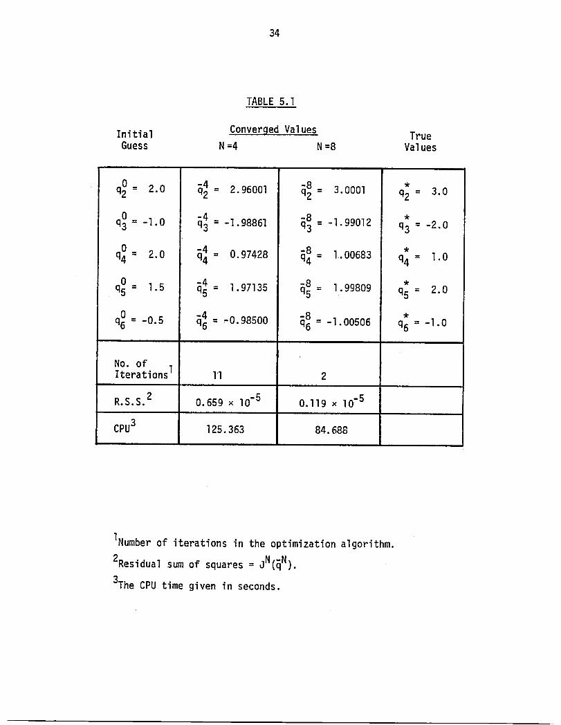
Example5.1. For our first examplewe used "data"consistingof observations
at x=O and times t = .25, .5, .75, ...,2.0. This is meant to simulatethe
situationin "surfaceseismic"experimentswhere only data at the surfaceare
available. The sourceterm was chosenas s(t;k)= q5(l-e-St)eq6t, a function
which rises to a peak quicklyand then graduallydiminishesto zero; again
this attemptsto mimic the situationin seismicexperiments. We assumevan-
ishinginitialconditionsand seek to estimatea constantelasticmodulusq2
as well as the boundaryparametersq3' q4 and the sourceparametersk= (qs,q6).
True valuesalong with our estimatesare given in the resultssummarizedin
Table 5.1. Graphs comparingthe true solutionat the surfaceu(t,O;q)with
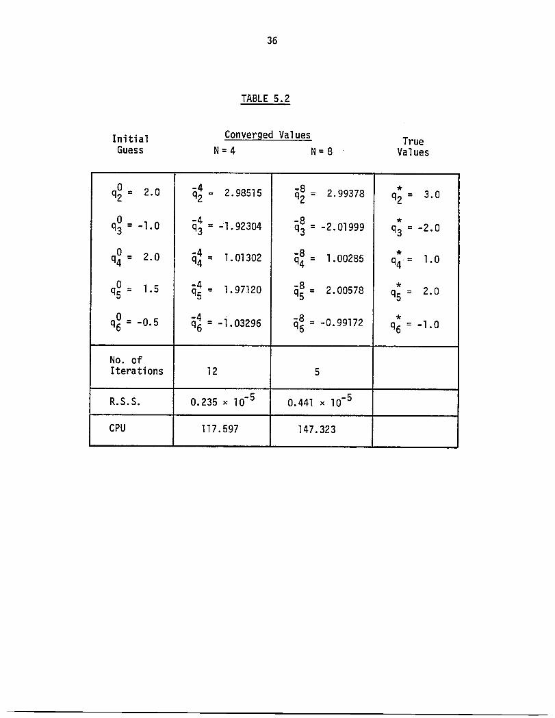
the approximatesolutionuN(t,O;qN) are shown in Figure5.1. We also tested
the methodon this exampleusing "data"for more spatialobservations(data
at x=O, .5, l.O and at t = .5, l.O, 1.5)with our findingsgiven in Table 5.2.
Based on these computationsand a numberof other tests,we suggestthat
there appearsto be littledifficultywith our method in the case where only one
spatialobservationis availableas long as a sufficientnumber of time
observationsare available.
34
TABLE5.1
Initial ConvergedValues TrueGuess N =4 N=8 Values
ii
q = 2.0 = 2.96001 = 3.0001 q2 = 3.0
q = -l.O = -I.98861 = -I.99012 q3 = -2.0
q = 2.0 = 0.97428 = 1.00683 q4 = l.O
q = 1.5 = 1.97135 = 1.99809 q5 = 2.0
q = -0.5 = -0.98500 = -I.00506 q6 = -l.O
No. ofIterationsI II 2
R.S.S.2 0.659 × lO-5 O.ll9 x lO-5
CPU3 125.363 84.688
INumberof iterationsin the optimizationalgorithm.
2Residualsum of squares= jN(_N).
3The CPU time given in seconds.

35
' u(t,O;q )
!
. u8(t,o;_8)
u(t,O;o*)
.l
#
.o
i
--, u8(t,o;58)t
i
ii
_!............ r'- ....................... _ ....... _ ............ ,'-_'_ . ,_., -_''r"-'- F
.... :_ " " ,? . _ ': 5 5.O
FIGURE 5.1
36
TABLE5.2
Initial ConvergedValues TrueGuess N = 4 N= 8 Values
q : 2.0 = 2.98515 : 2.99378 q2 = 3.0
q = -l.O = -I.92304 q_ = -2.01999 q3 = -2.0
q = 2.0 = 1.01302 = 1.00285 q4 = l.O
q = 1.5 = 1.97120 = 2.00578 q5 = 2.0
q = -0.5 = -i.03296 = -0.99172 q6 = -l.O
No. ofIterations 12 5
R.S.S. 0.235 × lO-5 0.441 x lO"5
CPU I17.597 147.323

37
Example5.2. In thisexample we comparedthe performanceof our method on
problemswith "noisydata" with that on those withoutnoise in the data. We
used the same source term as that in Example5.1, zero initialconditions,
but a "true"parameterizedelasticmodulusE(x) = 3/2 + I/_ Arctan [q21(x-q22)].
Data for observationsat x = 0.0, 0.5, l.O and t = .416, .832, 1.248, 1.664,
2.08, 2.496 were used. Resultsfor the case of data withoutnoise are summarized
in Table 5.3, while findingsemployingdata with a noise level of approximately
3% are given in Table 5.4. In both cases, the method convergesnicely but as
one might expect,the convergedvalues of the parametersdo not agree with the
true parametersin the case of noisy data. In Figures5.2, 5.3, 5.4 and 5.5,
we graphicallydepictedthe curvesfor _N and E in severalcases.
Example5.3. In this examplewe illustratethe ideasdiscussedin Section4
regardingparameterapproximationin the set of linearand cubic splines. We
do not assumean a priorishape for the elasticmodulus E(x), the "true"value
of which is given by E (x) = 3/2 + tanh [6(x-.5)]. Ratherwe first search,
for E in the class of linearsplineapproximationsto E . We then carry out
the searchusing cubic splines. Initialconditionsare u(O,x) = ex,
ut(O,x)= -3ex and no source termwas assumed(i.e., s_O). Data for observations
at 3 spatialpoints (x=O.O, 0.5, l.O) and 6 time points (t= .16, .32, ..., l.O)
were used. Figure 5.6 depictsgraphs of the true modulusE , the initialguess
EO, and the convergedestimate_4 where We used linearsplines (with4 basis
elements--M= 3 in the notationof Section4) to approximateE and cubic splines
(N= 4) to approximatethe state. At the same time we searchedfor the boundary
parametersq3' q4 (truevaluesq3 = -l.O, q4 = 3.0) and obtainedconverged

38
,TABLE5.3
Initial ConverqedValues TrueGuess N = 4 N = 8 Values
q l = l.O l = 2.97352 l = :2.99994 q21 = 3.,0
q 2 = l.O 2 = 0.511_5 2 = 0.50053 q22 = 0,'5
q = -2.0 = -0.99892 = -1.00026 q3 = -l.O
_ _ * _oq = 2.0 = 3.05138 = 3.,01,070 q4 =
o _ _ .q5 = l.O = 2.00322 = 2,00056 q5 = 2.0
q = -2.0 = -I.01163 _8 = -I.00217 q6 = -l.O
No. ofIterations 13 3
R.S.S. 0.I025 x lO-3 0.82859x lO-5
CPU 269.696 196.335

39
TABLE5.4
(NOISYDATA)
Initial ConvergedValues TrueGuess N = 4 N= 8 Values
l = l.O = 3.30536 q21 = 3.29222 q21 = 3.0
o Io _ = os38o2_ o o5311s*q22 = " 2 2 q22 = 0.5
q = -2.0 = -0.86648 = -0.86017 q3 = -l.O
q = 2.0 = 2.99610 = 2.96002 q4 = 3.0
q = l.O = 2.09207 = 2.09295 q5 = 2.0
q = -2.0 = -I.15602 = -I.15571 q6 = -l.O
No. ofIterations 13 2
R.S.S. 0.6509× 10⁻³ 0.476 x 10⁻³
CPU 270.II 136.87

18_ y17..,
1 6 ._.'_r_;4
o
1 4 .,., _,a_s°- _ _"_'- ,,_
1 2 . n
NONOISE
1 1T T l I I I t i I
0 0.1 0._- 0.3 0.4 0._ 0.6 0.? 0.8 0.9 I
X
FIGURE5.2

I
181
I?
16
14
13
12NO.NOISE
11I I I I I i i I I
0 0.1 0.'2 0.3 0.4 0.S 0.6 0.? 0.8 0.9 1
X
FIGURE5.3

1.?
1.2
NOISE!
X
FIGURE5.4

X
FIGURE5.5
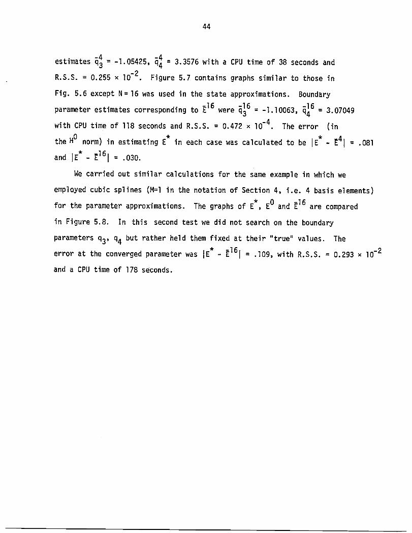
44
Aestimatesq_ = -I.05425,q_ = 3.3576with a CPU time of 38 secondsand
i
R.S.S.= 0.255 x lO-2. Figure 5.7 containsgraphs similarto those in
Fig. 5.6 exceptN= 16 was used in the state approximations. Boundary
parameterestimatescorrespondingto _16 were _6 = -I.I0063,_6 = 3.07049
with CPU time of ll8 secondsand R.S.S. = 0.472 × lO-4. The error (in
the H0 norm) in estimatingE in each case was calculatedto be IE* E41 = .081
and IE*- 161= .030.
We carriedout similarcalculationsfor the same examplein which we
employedcubic splines (M=lin the notationof Section4, i.e. 4 basis elements)
* E0 _16for the parameterapproximations. The graphsof E , and are compared
in Figure5.8. In this second test we did not searchon the boundary
parametersq3' q4 but rather held them fixed at their "true"values. The
error at the convergedparameterwas IE - El61 = .I09,with R.S.S.= 0.293 × lO-2
and a CPU time of 178 seconds.

.I:=,
_. EO
1 ...... - "_" EO ....
O.B _ - ..... N=4
M=3
0I | i i I I i i i
0 0.1 0,2 0.3 0.4 0,_ 0.8 0.7 0.8 0.9 1
X
FIGURE 5.6

2 E*--$__ "'__
.i'L_ 16
"'_ N=16
M=3
I I i I I I i i 1e e.1 o._- e.3 o.4 e._ e.6 e.? e.8 0.9 1
X
FIGURE 5.7

:3
1.5 _ ._"M
1
O.N- ......." N=I6
M=l
0I I I I I I I I
0 0.1 0.2 0.3 0.,4 0.5 0.6 0.'7' 0.8 0.9 1
X
FIGURE5.8
48
6. ConcludingRemarks.
We have presentedin this paper both theoreticaland numericalresults
using some of our ideas involvingspline approximationsfor inverseor
parameterestimationproblemsfor hyperbolicsystems. Among the novel features
is the capabilityof estimatingvariablecoefficientsand boundaryparameters
with methodsthat are both theoreticallysound and readilyimplementable.
Our techniques(reportedon earlier,[6]) involvethe use of parameterdependent
basis elementsfor the approximationsubspacesin a Galerkintype semi-discrete
scheme.
While we have focusedon l-dimensionalspace domainproblemshere, our
ideas.arein principleapplicableto problemsin 2 and 3 dimensionaldomains.
We have devotedsome thoughtto such problemsin connectionwith use of basis
elementsthat are tensor productsof l-D elements. These ideas offer some
promise,given the parallelismthat would be inherentin the resultingalgo-
rithmsand given the emergingtechnologyrelatedto supercomputersand array
processors. However,there are other ideas that also offer great promise;in
particular,there are those involvingspectralmethodssuch as the tau-Lege_drefor
which we have reportedpreliminaryfindingsin [4]. A fundamentaldifference
betweenthese techniquesand those proposedin this paper is that in the tau-
Legendreone does not requirethe approximationsubspacebasis elementsto
satisfythe boundaryconditions. Insteadthe boundaryconditionsare essen-
tially imposedas side constraintsadjoinedto the GalerRin type differential
equations. This can offer significantcomputationaladvantages,especially
in higherdimensionaldomain problems. We are currentlypursuinginvestigations
of these ideas.

49
In closingwe remarkthat the theoreticalresultspresentedabove only
guaranteeconvergenceof subsequences to a minimizerq for d. But for
the class of problemsinvestigatedhere and for a numberof other types of
inverseproblemswe have studied,we have in practiceonly observed (numerically)
convergenceof the originalsequence£qN_. This has been our experienceeven
in exampleswith noisy data and may be due in many cases to the fact that the^
originalproblemof minimizingJ over Q has a uniquesolutionq . In this
situation,elementaryand quite standardargumentscan be employedto actually
establishconvergenceof N itselfto q •
Acknowledgement.
The authorswould like to expresstheir sincereappreciationto G. Moeckel
(MobilOil Co.), R. Ewing (U. Wyoming),and K. Ku_isch(U. Graz) for
stimulatingdiscussionsduring the course of some of the work reportedabove.
They are also gratefulfor the supportand hospitalityreceivedduringtheir
visit at SouthernMethodistUniversitywhere a substantialportionof the
investigationsreportedon herewere carriedout.
50
References
I. A. Bamberger,G. Chavent,and P. Lailly,About the stabilityof theinverseproblemin l-D wave equations-applicationto the interpretationof seismicprofiles,Appl. Math. Optim. 5 (1979),p. 1-47.
2. H. T. Banks and J. M. Crowley,Parameterestimationfor distributedsystemsarisingin elasticity,Proc. Symposiumon EngineeringSciencesand Mechanics,(NationalCheng Kung University,Tainan,Taiwan,Dec. 28-31,1981),p, 158-177;(LCDSTech. Rep. 81-24,November,1981, Brown University).
3. H. T. Banks,J. M. Crowleyand K. Kunisch,Cubic splineapproximationtechniquesfor parameterestimationin distributedsystems. (LCDSTech.Rep. 81-25,November,1981, Brown University);IEEE Trans.Auto. Control.,AC-28 (1983),p. 773-786.
4. H. T. Banks,K. Ito and K. A. Murphy,Computationalmethodsfor estimationof parametersin hyperbolicsystems,in Conf. on InverseScattering:Theory and Application(J. B. Bednar,et.al, eds.),SIAM, Philadelphia,1983, p. 181-193.
5. H. T. Banks and K. Kunisch,An approximationthoeryfor nonlinearpartialdifferentialequationswith applicationsto identificationand control,SIAM J. Controland Optimization,20 (1982),p. 815-849.
6. H. T. Banks and K. A. Murphy,Inverseproblemsfor hyperbolicsystemswithunknownboundaryparameters,in ControlTheory for DistributedParameterSystemsand Applications(F. Kappel,et.al.,eds.),Springer-Verlag,Berlin,1983, p. 35-44.
7. H. T. Banks and I. G. Rosen,Fully discreteapproximationmethodsfor theestimationof parabolicsystemsand boundaryparameters,ICDS TechnicalReport No. 84-19, Brown University, 1984
8. K. P. Bube and R. Burridge, The one-dimensional inverse problem of reflectionseismology, SIAM Rev. 25 (1983), p. 497-559.
9. J. A. Burns and E. M. Cliff, An approximation technique for the control andidentification of hybrid systems, in Dynamics and Control of Larqe Flexibl_Spacecraft, 3rd VPISU/AIAA Symp., 1981, p. 269-284.
I0. G. Chavent, About the stability of the optimal control solution of inverseproblems, in Inverse and Improperly Posed Problems in Differential Equations,(G. Anger, ed.), Akademic-Verlag, Berlin, 1979, p. 45-58.
II. J. M. Crowley, Numerical methods of parameter identification for problemsarising in elasticity, Ph.D. Thesis, Brown University, May, 1982.
12. B. Engquist and A. Majda, Absorbing boundary conditions for the numericalsimulationof waves, Math. Comp.31 (1977),p. 629-651.

51
13. N. L. Guinassoand D. R. Schink,Quantitativeestimatesof biologicalmixing rates in abyssalsediments,J. Geophys.Res. 80 (1975),p. 3032-3043.
14. K. A. Murphy,A spline-basedapproximationmethod for inverseproblemsfor a hyperbolicsystem includingunknownboundaryparameters,Ph.D. Thesis,Brown University,May, 1983.
15. A. Pazy, Semigroupsof LinearOperatorsand Applicationsto PartialDifferentialEquations,App.Math Sciences,Voi..44,Springer,"NewYork,1983.
16. P. M. Prenter,Splinesand VariationalMethods,New York: Wiley-Interscience,1975.
17. R. D. Richtmyerand.K. W. Morton,DifferenceMethodsfor Initial-ValueProblems,NewYork: Wiley-Interscience,1967_
18. I. G. Rosen,Approximationmethodsfor the identificationof hybridsystemsinvolvingthe vibrationof beamswith tip bodies,CSDL-P-1893,CharlesStarkDraper Laboratory,Cambridge,MA.
19. M. H. Schultz,SplineAnalysis,EnglewoodCliffs,N.J.: Prentice-Hall,1973.
20. J. Storchand S. Gates,Planar dynamics,of a uniformbeam with rigidbodiesaffixedto the ends, CSDL-R-1629,Draper Labs, Cambridge,May, 1983.
21. E. Turkel,Numericalmethodsfor large-scaletime-dependentpartialdifferentialequations, in Comp. Fluid Dynamics(W. Kollmann,ed.),HemispherePubl.,Washington,1980, p. 127-262.


1. ReportNo. NASA CR-172389 2. GovernmentAccessionNo. 3. Recipient'sCatalogNo.ICASE Report No. 84-24
4. Title and Subtitle 5. Report DateEstimation of coefficients and boundary parameters June 1984
in hyperbolic systems 6. PerformingOrganizationCode
7. Author(s) 8. Performing Organization Report No,
H. Thomas Banks and Katherine A. Murphy 84-24
10. Work Unit No.9. Performing Organization NameandAddress
Institute for Computer Applications in Science
and Engineering '11. Contract or Grant No.
Mail Stop 132C, NASA Langley Research Center NASI-16394, NASI-17130
Hampton, VA 23666 13. Type of Report and Period Covered12. Sponsoring Agency Name and Address Contractor Report
National Aeronautics and Space Administration 14. Sponsoring AgencyCodeWashington, D.C. 20546 505-31-83-01
15. SupplementaryNotesAdditional Support: NSF Grant MCS-8205355, AFOSR Contract 81-0198,
and ARO Contract ARO-DAAG-29-83-K0029.
Langley Technical Monitor: Robert H. Tolson
W_n_1 R_nort16. Abstract
We considersemi-discreteGalerkinapproximationschemesin connectionwithinverseproblems for the estimationof spatiallyvarying coefficientsand boundaryconditionparametersin second order hyperbolicsystemstypicalof those arisinginI-D surfaceseismicproblems. Spline based algorithmsare proposedfor whichtheoreticalconvergenceresultsalong with a representativesample of numericalfindingsare given.
17. Key Words (Sugg_ted by Author(s)) 18. Distribution Statement '
parameter estimation 42 Geosciences (General)hyperbolicsystems 64 NumericalAnalysisapproximationtechniques
Unclassified- Unlimited
19. SecurityOassif.(ofthisreport) 20. SecurityClassif.(ofthispe_) 21. No. of Pages 22. DiceUnclassified Unclassified 53 A04
ForsalebytheNationalTechnicalInformationService,Springfield,Virginia 22161 NASA-Langley,1984


Top Related