


Languages
Pages
Legal


General rights Copyright and moral rights for the publications made accessible in the public portal are retained by the authors and/or other copyright owners and it is a condition of accessing publications that users recognise and abide by the legal requirements associated with these rights.
• Users may download and print one copy of any publication from the public portal for the purpose of private study or research. • You may not further distribute the material or use it for any profit-making activity or commercial gain • You may freely distribute the URL identifying the publication in the public portal
If you believe that this document breaches copyright please contact us providing details, and we will remove access to the work immediately and investigate your claim.
Downloaded from orbit.dtu.dk on: Aug 02, 2018
Heat Transfer Correlation in Nuclear Reactor Safety Calculations
Abel-Larsen, H.; Olsen, Aksel Aage; Miettinen, J.; Siikonen, T.; Rasmussen, J.; Sjöberg, A.; Becker, K.
Publication date:1985
Document VersionPublisher's PDF, also known as Version of record
Link back to DTU Orbit
Citation (APA):Abel-Larsen, H., Olsen, A. A., Miettinen, J., Siikonen, T., Rasmussen, J., Sjöberg, A., & Becker, K. (1985). HeatTransfer Correlation in Nuclear Reactor Safety Calculations. Nordic Liaison Committee for Atomic Energy.(Risø-M; No. 2504).

DtSfeoooia. - £ » * ! , fa, i j f
c"i «lt&fti ,iBte:. . * J "
» - * ;- <
»•T«" 9 P J J l ' l ¥•!#!;
*M
GDfe) Noidisk Nonfeka kotttktoigantof kontakkyganetlfr atomMnwga- fiasoncommneelor tfommcigisfMigsnål tfonwnaigiftigor yhdyMSn aktmcwMigy
RISØ-M-2504
HEAT TRANSFER CORRELATIONS IN
NUCLEAR REACTOR SAFETY CALCULATIONS
SAK-5
H. Abel-Larsen, Risø
A. J. T.
J. A. K.
Olsen,
Miettinen,
Siikonen,
Rasmussen,
Sjdberg,
Becker,
Risø
VTT VTT
IFE Studsvik
KTB
June 1985
Risø: Risø National Laboratory, Denmark
VTTJ Technical Research Centre of Finland
IFE: Institute for Energy Technology, Norway
Studsvik: Studsvik Energiteknik AB, Sweden
KTH: Royal Institute of Technology, Stockholm, Sweden
ISBN 87-550-1109-8 ISSN 0418-6435 mkmUgM* Stockholm 1MB
- 1 -
ABSTRACT
Heat transfer correlations, most of them incorporated in the
heat transfer packages of the nuclear reactor safety computer
programmes RBLAP-5, TRAC (PP1) and NORA have been tested
against a relevant set of transient and steady-state ex
periments. In addition to usually measured parameters the cal
culations provided information on other physical parameters.
Results are presented and discussed.
The report consists of a main report (Vol.I) and appendices
(Vol.II). Chapters 3,4 and 5 of the main report are primarily
intended for computer programme users. Chapter 6 is recommended
for those looking for main results rather than details. The
appendices will be useful for computer programme developers.
INIS descriptors;
CRITICAL HEAT FLUX - CONPARATIVB EVALUATIONS - CORRELATIONS -
COORDINATED RESEARCH PROGRAMS - DENMARK - DROPLETS - EVAPOR
ATION - FINLAND - FAILURES - FUEL ELEMENTS - FILM BOILING-
FORCED CONVECTION - HEAT TRANSFER - LOSS OF COOLANT - NORWAY -
N CODES - NUCLEATE BOILING - NATURAL CONVECTION - R CODES -
REACTOR SAFETY - SWEDEN - T CODES - TRANSIENT - TRANSITION
BOILING - THERMAL RADIATION
This report is part of the safety programme sponsored by
UK A, the Nordic Liaison Committee for Atomic Energy, 1981-85.
The project work has been partly financed by the Nordic
Council of Ministers.

- 2 -
LIST OP CONTENTS
VOLUME I: Page
ABSTRACT 1 SUMMARY 9 SAMMENFATNING (Danish summary) 13
1. INTRODUCTION 17
1.1. The aim of the project 17
1.2. Organisation of the report 17
1.3. Heat transfer regions 18
2. ORGANIZATION OF THE PROJECT 25
2.1. Participating organizations 25
2.2. Distribution of work 26
3. PRESENT KNOWLEDGE 27
3.1. General considerations 27
3.2. Beat transfer in different flow regions 28
4. COMPARISON OF CORRELATIONS WITH DATA 34
4.1. Computer programmes used 34
4.2. Comparisons with data 35
4.3. Experiences using the computer programmes 38
4.4. Comparisons using separate programmes 39
5. DISCUSSIONS AND RECOMMENDATIONS 41
5.1. Nucleate and forced convective boiling 41
5.2. Critical heat flux 42
5.3. Transition boiling 43
5.4. Rewetting 44
5.5. Film boiling 45
5.6. Interfacial heat transfer 48
6. CONCLUSION 52
NOMENCLATURE 55
- 3 -
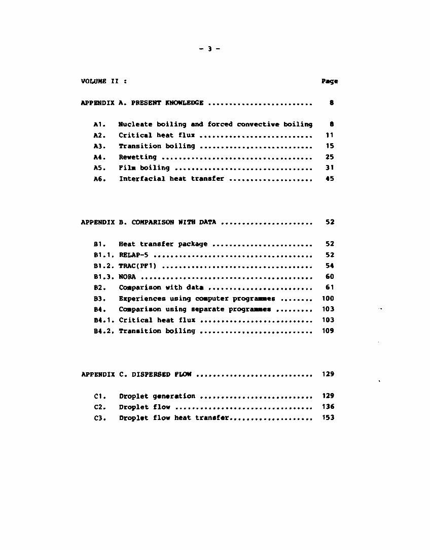
VOLUME II : Page
APPENDIX A. PRESENT KNOWLEDGE 8
A1. Nucleate boiling and forced convective boiling 8
A2. Critical heat flux 11
A3. Transition boiling 15
A4. Revetting 25
A5. Film boiling 31
A6. Inter facial heat transfer 45
APPENDIX B. COMPARISON WITH DATA 52
B1. Heat transfer package 52
B1.1. RELAP-5 52
B1.2. TRAC(PFI) 54
B1.3. NORA 60
B2. Comparison with data 61
B3. Experiences using computer programmes 100
B4. Comparison using separate programmes 103
B4.1. Critical heat flux 103
B4.2. Transition boiling 109
APPENDIX C. DISPERSED FLOW 129
CI. Droplet generation 129
C2. Droplet flow 136
C3. Droplet flow heat transfer 153

- 4 -
FIGURES. Page
VOLUME It
1. Boiling curve 19
2. Heat transfer regions 21
3. Beat transfer regions (T W<TCHP) 22
4. Beat transfer regions (Tw>TQgp) • 2 3
5. Beat t. .zfer nodes in two-phase flow 30
6. Critical heat flu« Mechanises 33
VOLUME lit
A3.1. Droplet deposition 22
A5.1. Flow transitions at CHP 41
A5.2. Types of inverted annular filn .. 42
AS.3. Comparison between Measured and calculated ...
results - heat transfer coefficient Bromley .. 43
A5.4. As above but Modified Bromley 44
A6.1. Pressure vs. tiMe. Comparison between Measured
and calculated results 50
A6.2. Critical Mass flux vs. pressure 51
A6.3. Critical Mass flus vs. pipe length 51
B1.1. Beat transfer coefficient surface using heat
transfer package of RELAP-5 with default CBF-
correlation 55

_ 5 -
Page
Bl.2. As B1.1 but Beckers CHP-correlation and void
limit excluded 56
B2.1. Roumy case 1 63
B2.2. Roumy case 2 64
B2.3. Mass flow vs. time 65
B2.4. CHP and heat rate vs. time 65
B2.5. Outlet wall temperature vs. time 66
B2.6. Mass flow vs. time 66
B2.7. CHP and heat rate vs. time 67
B2.8. Outlet wall temperature vs. time 67
B2.9. CE/EPRZ single tube blowdown loop 70
B2.10. Void vs. time 71
B2.11. Temperature vs. time 71
B2.12. Temperature vs. time 72
B2.13. Pressure vs. time 72
B2.14. Mass flux vs. time 73
B2.15. Power vs. time 73
B2.16. Outlet node void vs. time 74
B2.17. Outlet temperature vs. time ................. 74
B2.18. Wall temperature vs. time 75
- 6 -
Page
B2.19. Wall temperature vs. time 75
B2.20. Becker test section 80
B2.21. Temperature vs. length (NORA-case 1} 81
B2.22. Temperature vs. length (RELAP-5 case 1) 82
B2.23. Temperature vs. length (case 2) 83
B2.24. Temperature vs. length (case 3) 84
B2.25. Temperature vs. length (case 4) 85
B2.26. Temperature vs. length (case 7) 86
B2.27. Temperature vs. length (case 1 - new model)... 87
B2.28. Temperature vs. length (case 2) 88
B2.29. Temperature vs. length (case 3) 89
B2.30. Temperature vs. length (case 7) 90
B2.31. ORNL-64 rod test bundle 92
B2.32. Grid and thermocouples, axial location 93
B2.33. Temperature vs. length (case B) 94
B2.34. Temperature vs. length (case C) 95
B2.35. Temperature vs. length (case H) 96
B2.36. Temperature vs. length (case K) 97
B2.37. Temperature vs. length (case N) 98
B2.38. Temperature vs. length (case O) 99
B3.1. Velocity profiles in Becker case 1 104
B3.2. Calculated temperatures and vapour generation
rate Becker case 1 104
B3.3. Interfacial friction coefficient vs. void ... 105
B4.1.1. Local conditions hypothesis 111
B4.1.2. Comparison between measured and predicted ...
burnout power 112
B4.1.3. As above 113
B4.1.4. As above 114 B4.1.5. As above 115
- 7 -
Page
B4.1.6. Comparison between measured and predicted ...
dryout heat flux - OF 64 116
B4.2.1. Chen parameter B(P) vs. pressure 120
B4.2.2. Exponent in decay factor vs. wall superheat . 121
B4.2.3. Comparison-measured-predicted-transition
boiling heat transfer coefficient 124
B4.2.4. As above 125
B4.2.5. As above 126
B4.2.6. As above 127
B4.2.7. As above 128 C1.1. Droplet generation by entrainment 130 C2.1. Distribution coefficient for velocity and
void 152
TABLES
VOL.1:
4.2.1. Selected test cases 37
VOL. II:
A1.I. Pre-CHF two-phase heat transfer correlation.... 9
A1.II. As above 10
A2.I. CHF correlation tested by Leung 14
A2.II. Testing of CHF correlation 15
A3.I. Transition boiling heat transfer correlation .. 17-21
B4.1.I. RMS-errors obtained with the local hypothesis.. 110

- 8 -
Steering committee for the NKA/SAK reactor safety programme,
SAK-5 1981 - 1985:
C. Graslund
(Chairman)
Swedish Nuclear Power Inspectorate, SKI
Stockholm
T. Eurola Finish Centre for Radiation
and Nuclear Safety,
Helsingfors
E. Hellstrand Studsvik Energiteknik AB,
Nyk6ping, Sweden
D. Nalnes Institute for Energy Technology,
Norway
F. Marcus NKA,
Roskilder Denmark
B. Nicheeisen Risø National Laboratory,
Roskilde, Denmark
B. Sokolowski Nuclear Safety Board of
the Swedish Utilities,
Sverige

- 9 -
SUMMARY
Knowledge about temperatures on the surface of nuclear fuel
rods plays an important role in nuclear reactor safety analysis.
There is a need to calculate surface temperatures during opera
tional transients and postulated accidents under the assumption
that the engineered safety features of the reactor are activated
and working. A typical sequence to be calculated is a loss-of-
coolant accident (LOCA).
The purpose of the calculations is to examine whether the in
tegrity of the fuel rod cladding, the first of three engi
neered barriers against radiological release, may be threatened
by the rise in surface temperature that may occur.
The integrity of the cladding depends on several individual
phenomena, primarily metallurgical, all very sensitive to the
cladding temperature.
For this purpose thermo-hydraulic computer programmes have been
developed e.g. the American programmes TRAC and RBLAP-5 and the
Norwegian programme MORA, all used in the present project.
In order to calculate realistic temperature differences between
the cladding surface and the coolant, reliable heat transfer
correlations are needed for the different heat transfer regions
occuring during a transient (cf. the front page figure).
The heat transfer correlations actually used in the computer
programmes are empirical to a high degree. They have been
found from the results of independent steady-state experiments,
using boundary conditions, that coincide with boundary condi
tions in safety calculations only partly.
A comprehensive test program is therefore necessary to show
whether the computer programmes can provide reasonable simu
lations of well-defined experiments that are selected so that
their conditions may be comparable with those occurring in the
fuel element channels of a nuclear reactor.
- 10 -
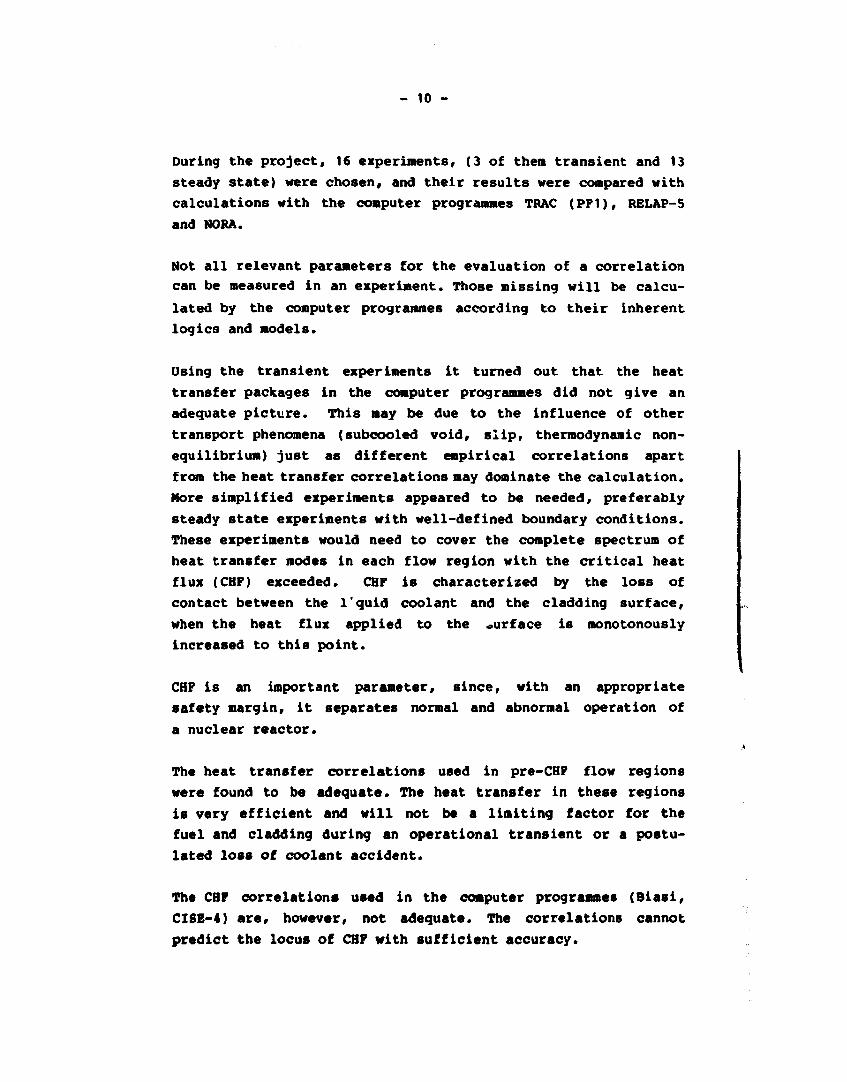
During the project, 16 experiments, (3 of them transient and 13
steady state) were chosen, and their results were compared with
calculations with the computer programmes TRAC (PPI), RELAP-5
and NORA.
Not all relevant parameters for the evaluation of a correlation
can be measured in an experiment. Those missing will be calcu
lated by the computer programmes according to their inherent
logics and models.
Using the transient experiments it turned out that the heat
transfer packages in the computer programmes did not give an
adequate picture. This may be due to the influence of other
transport phenomena (subcooled void, slip, thermodynamic non-
equilibrium) just as different empirical correlations apart
from the heat transfer correlations may dominate the calculation.
More simplified experiments appeared to be needed, preferably
steady state experiments with well-defined boundary conditions.
These experiments would need to cover the complete spectrum of
heat transfer modes in each flow region with the critical heat
flux (CHF) exceeded. CHF is characterized by the loss of
contact between the l'quid coolant and the cladding surface,
when the heat flux applied to the surface is monotonously
increased to this point.
CHF is an important parameter, since, with an appropriate
safety margin, it separates normal and abnormal operation of
a nuclear reactor.
The heat transfer correlations used in pre-CHF flow regions
were found to be adequate. The heat transfer in these regions
is very efficient and will not be a limiting factor for the
fuel and cladding during an operational transient or a postu
lated loss of coolant accident.
The CHF correlations used in the computer programmes (Biasi,
CISB-4) are, however, not adequate. The correlations cannot
predict the locus of CHF with sufficient accuracy.
- 11 -
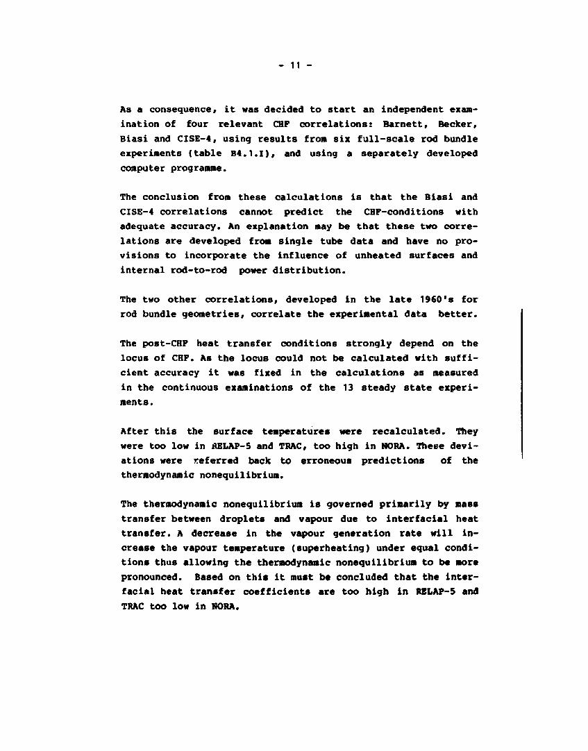
As a consequence, it was decided to start an independent exam
ination of four relevant CHP correlations: Barnett, Becker,
Biasi and CISE-4, using results from six full-scale rod bundle
experiments (table B4.1.I), and using a separately developed
computer programme.
The conclusion from these calculations is that the Biasi and
CISE-4 correlations cannot predict the CHP-conditions with
adequate accuracy. An explanation may be that these two corre
lations are developed from single tube data and have no pro
visions to incorporate the influence of unheated surfaces and
internal rod-to-rod power distribution.
The two other correlations, developed in the late 1960's for
rod bundle geometries, correlate the experimental data better.
The post-CHP heat transfer conditions strongly depend on the
locus of CHP. As the locus could not be calculated with suffi
cient accuracy it was fixed in the calculations as measured
in the continuous examinations of the 13 steady state experi
ments.
After this the surface temperatures were recalculated. They
were too low in AELAP-5 and TRAC, too high in NORA. These devi
ations were referred back to erroneous predictions of the
thermodynamic nonequilibrium.
The thermodynamic nonequilibrium is governed primarily by mass
transfer between droplets and vapour due to interfacial heat
transfer. A decrease in the vapour generation rate will in
crease the vapour temperature (superheating) under equal condi
tions thus allowing the thermodynamic nonequilibrium to be more
pronounced. Based on this it must be concluded that the inter
facial heat transfer coefficients are too high in RBLAP-5 and
TRAC tOO low in NORA.

- 12 -
A recently developed semi-empirical vapour generation model
was therefore implemented in the programmes. Hereafter, the
results were substantially improved, and a better agreement was
obtained between measured and calculated post-CHF surface temp
eratures.
It is obvious even from these last few calculations, together
with the examinations of transition boiling heat transfer using
a separately developed programme, that more realistic and phe-
nomenological heat transfer models have to be developed for the
post-CHF regions. It is recognized that the degree of thermo
dynamic nonequilibrium at any axial level will depend on the
upstream competition between the heat transfer mechanisms wall-
to-vapour by convection, wall-to-droplet by droplet impingment
on the surface and vapour-to-droplet by interfacial heat trans
fer.
The present project has been limited to application of the heat
correlations in nuclear reactors. However, the same basic
technical questions concerning heat transfer in fluids with
droplets or particles and the correlations used to descibe the
heat transfer find wide application in a number of fields
such as chemical processes, fluidized bed combustion, spray
cooling, heat and mass transfer in evaporators, once-through
steam generators to name a few.
The problems described in this report are an example of how
advanced methods developed for the nuclear area can contribute
to other technical areas of current interest.
- IS
SAMMEHFATMHG
Uranbrændslet i »n kernøkraftrøaktor ør stærkt radioaktivt. Det er vigtigt, at brxndelet indesluttes effektivt, så ingen radioaktive stoffer kan frigøre» til omgivelserne. Tre konstruerede barrierer tjener dette formal. De tre barrierer er først indkapslingen, der indeslutter det nukleare brændsel, dernæst reaktortanken, der omslutter reaktorkernen og dat primære kølesystem og endelig døn tryktætte reaktorbygning, der indslutter reaktoranlægget» primære systemer.
Et vigtigt led i sikkerhedsanalysen af kernekraftreaktorer er at eftervise, at temperaturerne på overfladen af indkapø-lingen under unormale driftsforstyrrelser og påstulerede u-held, som f.ek». tab-af-kølemiddel-uheld, ikke overstiger en fastsat værdi, når reaktoranlægget» beskytteeessy»terner virker.
Overetiger indkapsling sling »temperaturen den fastsatte grænseværdi kan indkapslingen revne. Ar»agen hertil er flare metallurgisk» fænomener alle føleomme overfor temperaturen.
Den absolutte »tørrøl»» af temperaturen afhænger af del», hvor godt man kan beet emme de metallurgieke fænomener» temperaturafhængighed og del», hvor godt *an kan bestemme indkapslingen» overfladetemperatur.
Projektet har beskæftiget sig med øen »ide af sidstnævnte punkt.
Beregning af realistiske temperaturforekellø mellem indkapslingens ovørflads og kølemidlet forudsætter pålidelige varme -overgangekorrelationer. Ved en korrelation »kal hør foretå» et matematiek udtryk, der nok etøttør »ig til fysiske principper, men primært er baeeret på »tati»ti»k behandling af foreøgedata.
- 14 -
Døt primærø formål mød nærværende projekt var at undereøge pålideligheden af nogle udvalgte korrelationer for varmetrane-porten med henblik på deres anvendelse i datamaskine-programmør, dør modellerer forholdene i reaktorkernen under et uheldsforløb.
St eksempel på en brændelsstavs overfladetemperatur undet såvel normal drift som under øt uheldsforløb ør givøt på forsidøn af dønne rapport. Kølemidlet er kogøndø vand, d.v.s. dør ør bådø damp og vand tilstøde (to-fase køling).
Vød normal drift af en kernekraftreaktor ekal overfladetemperaturen af indkapølingen holdes under den tømpøratur, dør svarer til den kritiekø varmestrøm (punkt C på forsidøfigurøn).
Undersøgelsen af de korrelationer, som anvendøe vød bestemmelsen af varmetransporten før kritisk varmestrøm, bekræftede, at de er tilstrækkelig pilidelige. Varmetransporten her er meget efføktiv og vil ikkø være en begrænsende faktor for indkapslingen.
Kritisk varmøøtrøm ør karakterisøret vød tabøt af kontakt mellem indkapslingens overflade og kølevand på grund af dannelsen af et overhedet lag af damp.
De korrelationer, som blev benyttet til beetemmelee af værdien af og øtødøt for kritiøk varmøøtrøm i dø anvendte datamaskine-programmer var ikkø tiløtrækkølig pålidøligø. En uafhængig undøreøgøløø mød øt øøparat udvikløt program bløv dørfor udført på dølø dø to anvøndtø korrelationer og dels to andrø, ældrø korrølationør. Hø sult at et var, at de to ældre korrelationer bødrø kunnø forudøigø forøøgødata fra 6 forøøg mød øløktriøk opvarmødø brændeelselementer i fuldskala.
Undereøgeleen af korrølationør for varmøtransportsn øf tør kritiøk varmøøtrøm vi øer, at dø tilstrækkølig pålideligt kan eftervise måltø overfladetemperaturer i dø forøøg, øom ør beny'tet vød sammønligningøn, når dør tagøø nødvøndigt hønøun til to fyøiøkø fænomenør:
- 75 -
J. termodynamisk uligevægt S. dråbekøling.
Ved den termodynamiske uligevægt skal forstås, at damptemperaturen, efter at den kritiske varmestrøm er passeret, kan blive højere e.J vandtemperaturen, idet varmetransporten primært vil ske til dampen og herfra videre til vanddråber i dampen. Dampen overhedes d.v.s. varmetransporten til dråber er ikke i ligevægt med varmetransporten til dampen. Ved at tage hensyn til denne overhedning kunne en væsentlig bedre overensstemmelse mellem forsøgsdata og beregnede overfladetemperaturer opnås.
Resultaterne fra undersøgelsen af termodynamisk uligevægt og resultater fra undersøgelsen af den såkaldte transition-kogning (området mellem punkterne C og D på forsidefiguren) viser, at dråbekølingen er et særdeles vigtigt led i varmetransporten.
Ved transitionkogning er varmetransporten bedre end i området for filmkogning (området mellem D og B på forsidefiguren), fordi dråber, som rammer indkapslingens overflade, kan væde overfladen. Kølingen forstærkes ved direkte fordampning af dråberne.
De to nævnte fænomener afhænger stærkt af hinanden, idet graden af den termodynamiske uligevægt vil afhænge af konkurrencen mellem varmetransporten: indkapelingeoverflade til damp ved konvektion, indkapelingeoverflade til dråber ved fordampning og endelig damp til dråber ved såkaldt interfase varmeovergang.
Undersøgelserne i SMK-S projektet har klarlagt dråbernes betydning for varmetraneporten i områderne efter kritisk varmestrøm. Man har vist, at om man vil forbedre pålideligheden er det nødvendigt at inddrage de fysiske fænomener mere d.v.s., der bør udvikløe mere realistiske modeller, eom i højere grad basøres på de fyeieke fænomener end korrelationerne er. Det ekal dog bemærkee, at fænomenologiske modeller, der kan bestå af flere matematiske udtryk, kan øge kompleksiteten af beregningsprogrammet og beregningstiden, ft valg mellem den detaljerede fæno-menologieke model og den statistiske korrelation kan derfor blive

- 16 -
nødvøndig.
Undaraøgalaørnø kar værøt bøgrænøøt til varmøtranaport i karna-
kraftrøaktorør, møn dø grundlæggøndø fyøiøkø og tøkniøkø øpørgø-
mål ør dø øammø for varmøtran»port indønfor øtorø områdør af
døn modørnø taknikt dør aåladaa ogaa kan dragø nytta af undar -
øøgølaørnø.

17 -
1. INTRODUCTION
1.1. The ail of the project
The aim is to establish a set of reliable heat transfer corre
lations primarily for application in best-estimate computer
programmes for nuclear reactor safety calculations.
Correlations in this sense are sets of mathematical expressions,
based on physical principles and experimental data, but resting
primarily on experimental data.
A best estimate is the most favourable with respect to reality.
Favourable is in this context according tj use and best know
ledge .
Reality refers to those transients that have to be evaluated
to assure the authorities that the safety of the system is
acceptable. The transients are all expected operational tran
sients and postulated accidents such as a break in the pressure
boundary integrity resulting in a loss of core cooling water
(Loss-of-Coolant-Accident, LOCA).
1.2. Organisation of the report
This report contains a main report (VOL.i) and appendices (VOL.il)
The main report covers the examined area from a more general
point of view. It provides a natural introduction to the appen
dices, which describe the work done in detail.
The participating organizations and the actual distribution of
the work are dealt with in Chapter 2.
- 18 -
The project was initiated with a literature search. The general
considerations and results are discussed in Chapter 3 and
Appendix A.
The comparison of selected heat transfer correlations with ex
perimental data using the American computer programmes RBLAP-5,
TRAC(PPl), the Norwegian coaputer programme MORA, and separate
programmes developed especially for this project is described
in Chapter 4 and Appendix B.
Discussions and recommendations based on the results attained
are given in Chapter 5.
Chapter 6 contains the conclusion of the report.
1.3. Beat transfer regions
The heat transfer correlations are closely connected with the
actual tlow region. The expressions flow region and heat trans
fer region may therefore be interchangeable.
The heat transfer regions and their occurrence in light water
reactors may be demonstrated by considering the temperature
course that a local spot on a heat transfer surface may experi
ence during a LOCA.
An example of such a temperature course as function of surface
heat flux is shown in Fig. 1, the so-called boiling curve.
The course from A to B represents the single-phase liquid flow
region. In the succeeding boiling region two different modes
of flow can occur. In one mode, the nucleate boiling mode,
the liquid is the continuous fluid; vapour is generated at
specific nucleation sites on the heating surface and vapour
bubbles are discretely distributed through the continuous,
saturated liquid phase (liquid continuous). The other mode,
the forced convective boiling mode, is characterised by the
vapour as being the continuous fluid with the liquid distributed
partly as a film on the heating surface and partly as droplets
in the vapour (vapour continuous).

_ 19
d o
Hl O.
u o <
CO
SURFACE HEAT FLUX (LOG.)
BORJNQ CURVE O H * Flux ControRwO

- 20 -
Nhen the heat flux applied to the surface in contact with the
liquid is progressively increased« a point is reached at which
the continuous contact between the surface and the liquid is
lost and the critical heat flux (CHF) is attained.
The teaperature course in Pig. 1 is shown for a heat flux-con
trolled surface* i.e. the heat flux is the independent variable
as in electric and nuclear-heated systeas.
When the surface heat flux in a heat flux-controlled systea
is further increased the teaperature will juap to point B. This
teaperature increase aay cause a burnout in the real sense of
the word and a certain safety aargin to the CHF point has to be
secured during noraal operation of a nuclear reactor.
The surface teaperature aay go froa P to B and further to D by
decreasing the heat flux. The teaperature at D is the so-called
ainiaua fila boiling teaperature. Proa here the teaperature aay
juap to the nucleate boiling, i.e. a fora of hysteresis effect
aay exist.
During a strong transient* such as a LOCA, the fuel rods aay
behave as a teaperature-controlled systea due to their theraal
capacities. The teaperature course can then aove into the
transition boiling flow region (froa C to D), where the heat
transfer is auch better than in the fila boiling flow region
(froa D to B and P).
The transition boiling flow region is active between the teape
rature at CHP and the ainiaua fila boiling teaperature and can
be realized only in teaperature-controlled systeas.
The flow regions as they aay occur in eaergency core cooling by
reflood is shown in Pig. 2.
In general the logic in the selection of the heat transfer cor-
lations aay appear froa these thoughts. Pigures 3 and 4 show
the aain features of the selection.

- 21 -
« "».
o e
• a
O • «
W
' • c v ' •
• * •
O • i •
* , '
# • 9
Dispersed Flow Fil« Boiling
Inverted Annular Fil« Boiling
L Transition Boiling
Nucleate Boiling
Single Phase Liquid
Dispersed Flow Fil« Boiling
Transition Boiling
Forced Convective Flow Boiling
Nucleate Boiling
Single Phase Liquid
HEAT TRANSFER RE6I0NS
FIGURE 2

- 22 -
£> LU LU •—•
o o o l i - «_>CO
O t—
o-—iz ~ _ * o - I U . U
CO
o c_>
</>
o z o LU LU
_ I O h O O Z « t Z 0 « u i « <_> 1 > i m •—<_> ~ =»o = o LO OD Z OD
LU O _ l U J — i
5S2
HEAT TRANSFER REGIONS
FIGURE 3

3 CD »Ml
YES
V
YES
TRANSITION BOILING LOW QUALITY
YES
INVERTED ANNULAR FILM BOILING
NO
YES
TRANSITION BOILING HIGH QUALITY
NO
NO
YES
DISPERSED DROPLET FLOW
SINGLE PHASE VAPOUR
N> Ul

- 24
Prom what is stated above, the heat transfer during the whole
temperature course can be traced to be dependent primarily on
the surface temperature and secondarily on whether the flow is
liquid continuous or vapour continuous.
The transport equation of heat, first set up by Newton in 1701,
is written:
Q - h»A«aT ,
where Q is the heat flow rate, A a characteristic surface area,
AT a characteristic temperature difference, and the proportiona
lity factor h is defined as the heat transfer coefficient.
The heat transfer coefficient depends on the physical proper
ties of the fluid, mass flux, pressure, absolute vapour quality
and the geometry of the system.
- 25 -
2. ORGANIZATION OF THE PROJECT
The project is part of the safety programme of NKA, the Nordic
Liaison Committee for Atomic Energy and is in part financed by
funds from the Nordic Council of Hinisters.
2.1. Participating organizations
The participants have been:
Rise National Laboratory, Denmark
H. Abel-Larsen
A. Olsen (project leader),
Technical Research Centre of Finland, VTT,
J. Niettinen,
T. Siikonen,
Institute for Energy Technology, IFE, Norway,
J. Rasmussen,
Studsvik Energiteknik AB, Studsvik, Sweden,
A, Sjdberg,
Royal Institute of Technology, KTH, Sweden,
Department of Nuclear Energy,
K.M. Becker.

- 26 -
2.2. Distribution of work
The logic classification of the boiling curve has been used as
a base for the initial distribution of work in the literature
search.
IFE has exaained the single phase liquid and the nucleate boil
ing and forced convective boiling flow region including the
critical heat flux.
Risø has exaained the transition boiling flow region.
Studsvik exaained the fila boiling and single phase vapour flow
region.
VTT exaained the quenching phenoaena during the eaergency core
cooling through top-spray and bottoa-reflooding and the inter-
facial heat transfer.
Professor Becker has taken part in the project since January
1983 as a consultant.

- 27 -
3. PRESENT KNOWLEDGE
The result of a literature search is given in Appendix A. Below
is given a general view of the transport phenomena of heat for
the physical understanding of the heat transfer and its corre
lation.
3.1, General considerations
Some basic criteria and general requirements for the selection
of heat transfer correlation may be set up as follows (1):
a. The range of the experimental data base on which
the correlation is based must coincide with the
range of interest.
b. The deviation of the predicted results with the cor
relation from the experimental data should be low,
i.e. a correlation with a lower standard deviation
should be selected over another correlation with
higher standard deviation.
c. If a. and b. are satisfied, the correlation based on
phenomenological or mechanistic considerations should
be preferred to the purely statistical correlation.
The phenomenological correlation may offer the possibility of
extrapolation outside the range of the data it is tested against
and further it may be possible to gain a better understanding
of the physical processes involved.
Phenomenological correlations often consist of various math
ematical expressions based on primarily physical principles.
The phenomenological model may, however, increase the complexity
of the computer programme management and increase the use of
28 -
computer tiae. A compromise between the detailed phenomenological
model and the statistical correlation may therefore be necess
ary. This depends primarily on the sensitivity of the surface
temperature to the selected correlation. If the sensitivity is
low, it aay be justifiable to lower the complexity.
h key feature of a well-made computer prograame is a high degree
of modularity so that correlations and models can be easily
changed.
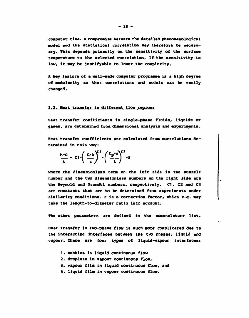
3.2. Heat transfer in different flow regions
Heat transfer coefficients in single-phase fluids, liquids or
gases, are determined from dimensional analysis and experiments.
Heat transfer coefficients are calculated from correlations de
termined in this way:
where the dimensionless term on the left side is the Husselt
number and the two diaensionless nuabers on the right side are
the Reynold and Prandtl nuabers, respectively. CI, C2 and C3
are constants that are to be determined from experiments under
siailarity conditions. P is a correction factor, which e.g. aay
take the length-to-diameter ratio into account.
The other paraaeters are defined in the nomenclature list.
Beat transfer in two-phase flow is auch more complicated due to
the interacting interfaces between the two phases, liquid and
vapour. There are four types of liquid-vapour interfaces:
1. bubbles in liquid continuous flow
2. droplets in vapour continuous flow,
3. vapour film in liquid continuous flow, and
4. liquid film in vapour continuous flow.
- 29 -
Further, the three different types of heat transfer have to be
considered:
a. convection
b. conduction, and
c. radiation.
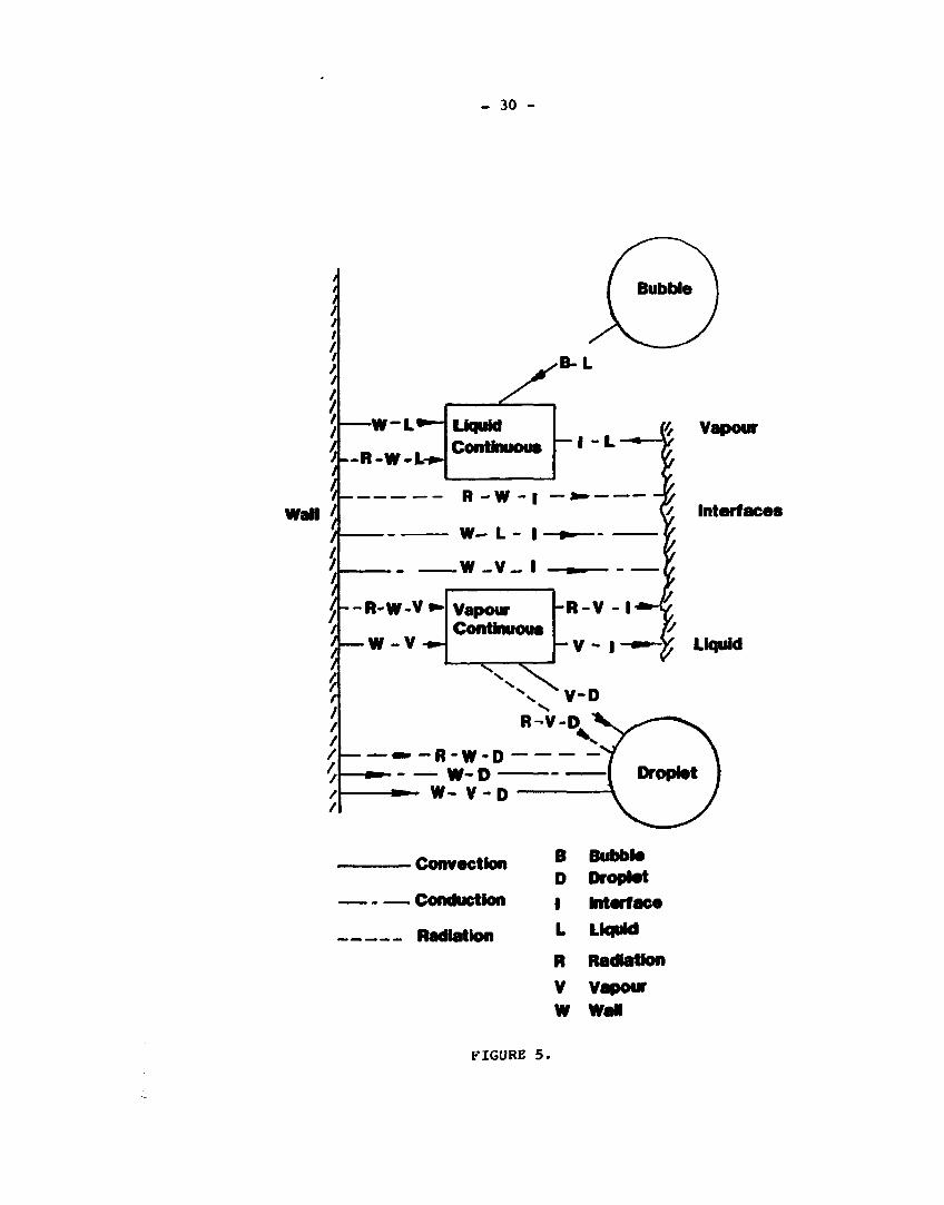
Pigure 5 gives schematically an impression of the highly com
plex aechanisas involved in the two-phase flow heat transfer.
It is understandable that it is not possible to obtain a single
heat transfer correlation that aay cover all the flow regions
shown in Fig. 1 and schematically in Pigs. 3 and 4.
Kot all the heat transfer aechanisas occur at the saae tiae and
they differ radically in the various flow regions. In aost
cases the thermal radiation is negligible.
To a great extent, the physical considerations froa structuring
single-phase heat transfer correlations have been transferred
to two-phase flow with appropriate additions even for inter-
facial heat transfer.
Superposition of the different heat transfer aechanisas is as
sumed. Nucleate boiling heat transfer, e.g., is correlated as
the sum of the heat transfer by liquid-vapour exchange caused
by bubble agitation in the boundary layer (aicroconvection) and
the heat transfer by the single-phase liquid convection between
patches of bubbles (macroconvection). Appropriately determined
weighing factors are assigned to each term.
In the post-CHP regions with vapour continuous flow the heat
transfer is very much dependent on the droplet concentration
and the surface temperature. At relatively low temperatures the
droplets will be able to wet the heating surface when striking
it and thus can be evaporated by direct contact with the sur
face. The heat transfer may be assumed to be a weighted sum of
- 30 -
Wall /
Vapour
/ Interfaces
Liquid
-Convection
Conduction
Radiation
B Bubble D Droplet I Interface L Liquid R Radiation
V Vapour W Wan
FIGURE 5 .
- 31 -
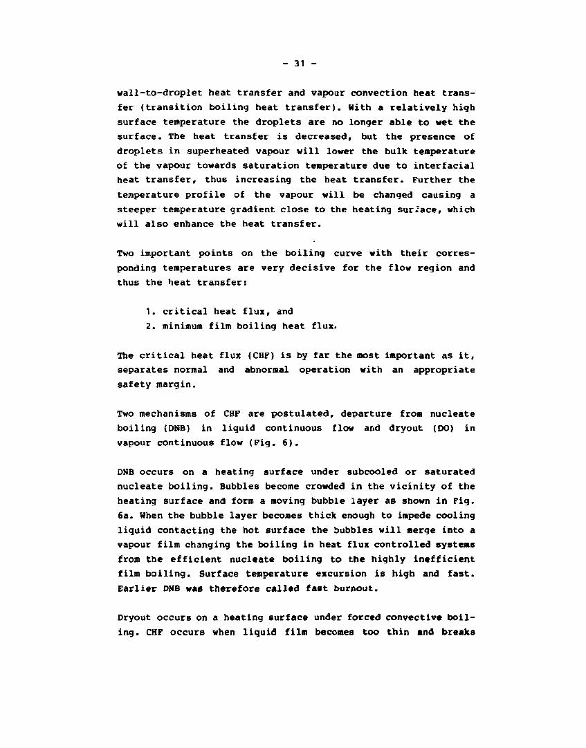
wall-to-droplet heat transfer and vapour convection heat trans
fer (transition boiling heat transfer). With a relatively high
surface temperature the droplets are no longer able to wet the
surface. The heat transfer is decreased, but the presence of
droplets in superheated vapour will lower the bulk temperature
of the vapour towards saturation temperature due to interfacial
heat transfer, thus increasing the heat transfer. Further the
temperature profile of the vapour will be changed causing a
steeper temperature gradient close to the heating surface, which
will also enhance the heat transfer.
Two important points on the boiling curve with their corres
ponding temperatures are very decisive for the flow region and
thus the heat transfer:
1. critical heat flux, and
2. minimum film boiling heat flux.
The critical heat flux (CHF) is by far the most important as it,
separates normal and abnormal operation with an appropriate
safety margin.
Two mechanisms of CHF are postulated, departure from nucleate
boiling (DNB) in liquid continuous flow and dryout (DO) in
vapour continuous flow (Fig. 6).
DNB occurs on a heating surface under subcooled or saturated
nucleate boiling. Bubbles become crowded in the vicinity of the
heating surface and form a moving bubble layer as shown in Fig.
6a. When the bubble layer becomes thick enough to impede cooling
liquid contacting the hot surface the bubbles will merge into a
vapour film changing the boiling in heat flux controlled systems
from the efficient nucleate boiling to the highly inefficient
film boiling. Surface temperature excursion is high and fast.
Earlier DNB was therefore called fast burnout.
Dryout occurs on a heating surface under forced convective boil-
ing. CHF occurs when liquid film becomes too thin and breaks
- 32
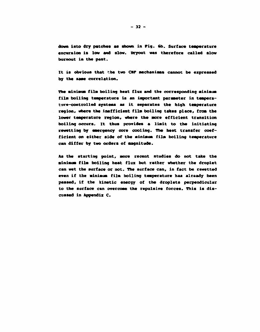
down into dry patches as shown in Pig. 6b. Surface teaperature
excursion is low and slow. Dryout was therefore called slow
burnout in the past.
It is obvious that the two CHP aechanisas cannot be expressed
by the saae correlation.
The ainiaua fila boiling heat flux and the corresponding ainiaua
fila boiling teaperature is an iaportant paraaeter in teapera-
ture-controlled systeas as it separates the high teaperature
region, where the inefficient fila boiling takes place, froa the
lower teaperature region, where the aore efficient transition
boiling occurs. It thus provides a liait to the initiating
rewetting by eaergency core cooling. The heat transfer coef
ficient on either side of the ainiaua fila boiling teaperature
can differ by two orders of aagnitude.
As the starting point, aore recent studies do not take the
ainiaua fila boiling heat flux but rather whether the droplet
can wet the surface or not. The surface can, in fact be revetted
even if the ainiaua fila boiling teaperature has already been
passed, if the kinetic energy of the droplets perpendicular
to the surface can overcome the repulsive forces. This is dis
cussed in Appendix C.

- 33 -
iDryout
Liquid ~Aimuhis
B
Two postulated Mechanisms of CHF
A: Departuro from Nucleate
BoMng (DNB)
Efc Departuro from Forced ConvectJve
BoMng (DFCB) or Dryout.
\ f
\
i
PIGURE 6.
- 34 -
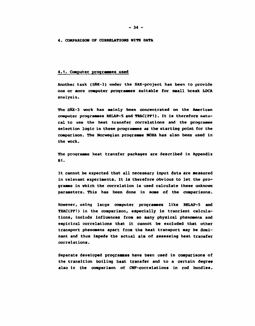
4. COMPARISON OP CORRELATIONS WITH DATA
4.1. Computer program* es used
Another task (SAK-3) under the SAK-project has been to provide
one or more computer programmes suitable for saall break LOCA
analysis.
The SXK-3 work has mainly been concentrated on the American
computer programmes RBLAP-5 and TRAC(PPl). It is therefore natu
ral to use the heat transfer correlations and the prog ramie
selection logic in these programmes as the starting point for the
comparison. The Norwegian programme NORA has also been used in
the work.
The programme heat transfer packages are described in Appendix
B1.
It cannot be expected that all necessary input data are Measured
in relevant experiments. It is therefore obvious to let the pro
gramme in which the correlation is used calculate these unknown
parameters. This has been done in some of the comparisons.
However, using large computer programmes like RBLAP-5 and
TRAC(PF1) in the comparison, especially in transient calcula
tions, include influences from so many physical phenomena and
empirical correlations that it cannot be excluded that other
transport phenomena apart from the heat transport may be domi
nant and thus impede the actual aim of assessing heat transfer
correlations.
Separate developed programmes have been used in comparisons of
the transition boiling heat transfer and to a certain degree
also in the comparison of CHP-correlations in rod bundles.
- 35 -
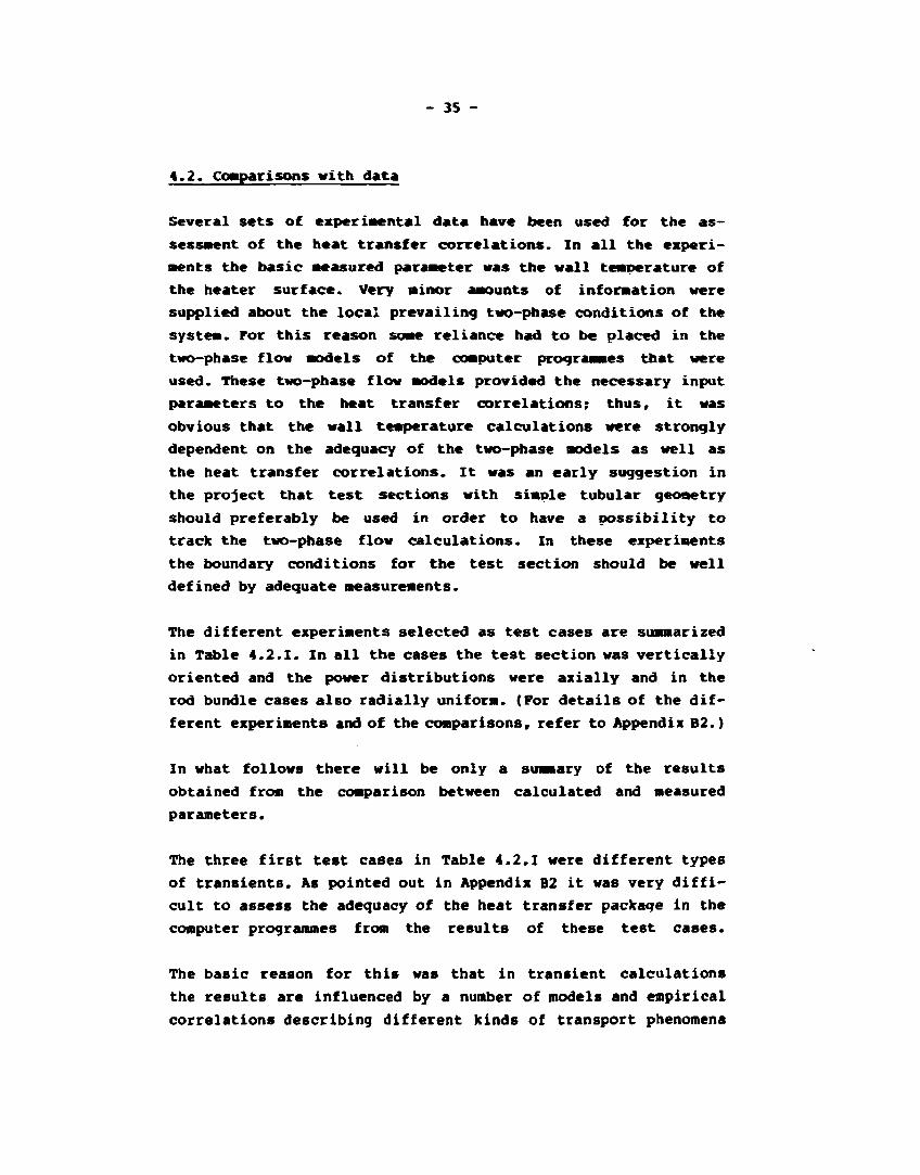
4.2. Comparisons with data
Several sets of experimental data have been used for the as
sessment of the heat transfer correlations. In all the experi
ments the basic measured parameter was the wall temperature of
the heater surface. Very minor amounts of information were
supplied about the local prevailing two-phase conditions of the
system. Por this reason some reliance had to be placed in the
two-phase flow models of the computer programmes that were
used. These two-phase flow models provided the necessary input
parameters to the heat transfer correlations; thus, it was
obvious that the wall temperature calculations were strongly
dependent on the adequacy of the two-phase models as well as
the heat transfer correlations. It was an early suggestion in
the project that test sections with simple tubular geometry
should preferably be used in order to have a possibility to
track the two-phase flow calculations. In these experiments
the boundary conditions for the test section should be well
defined by adequate measurements.
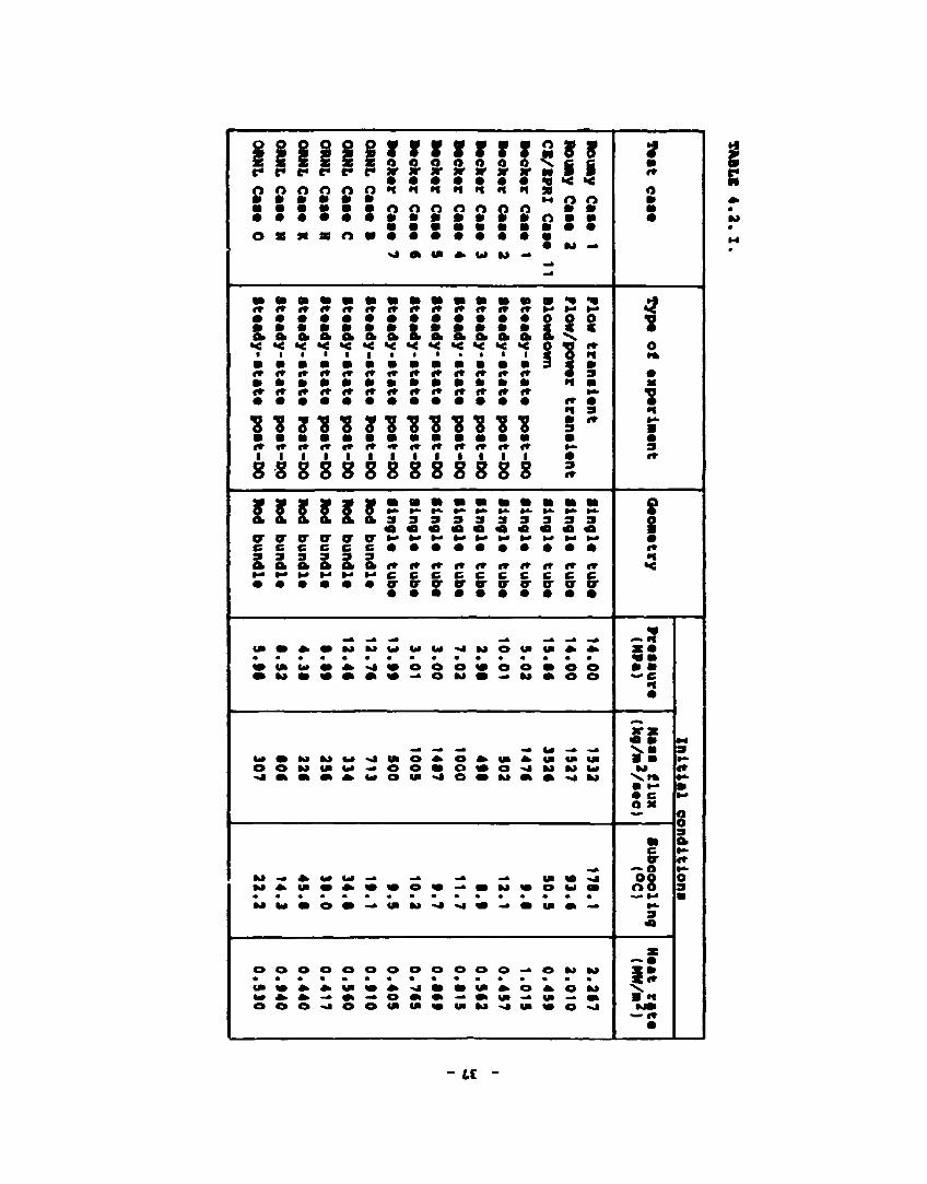
The different experiments selected as test cases are summarized
in Table 4.2.1. In all the cases the test section was vertically
oriented and the power distributions were axially and in the
rod bundle cases also radially uniform. (Por details of the dif
ferent experiments and of the comparisons, refer to Appendix B2.)
In what follows there will be only a summary of the results
obtained from the comparison between calculated and measured
parameters.
The three first test cases in Table 4.2.1 were different types
of transients. As pointed out in Appendix B2 it was very diffi
cult to assess the adequacy of the heat transfer package in the
computer programmes from the results of these test cases.
The basic reason for this was that in transient calculations
the results are influenced by a number of models and empirical
correlations describing different kinds of transport phenomena
- 3« -
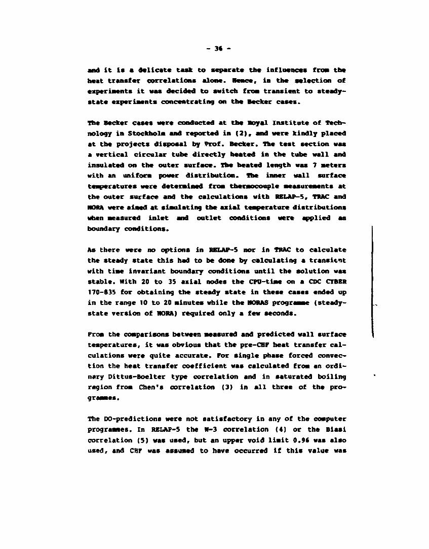
and it is a delicate task to separate the influences from the
heat transfer correlations alone, Bence, in the selection of
experiments it was decided to switch fron transient to steady-
state experiments concentrating on the Becker cases.
The Becker cases were conducted at the Royal institute of Tech
nology in Stockholm and reported in (2), and were kindly placed
at the projects disposal by Prof. Becker. The test section was
a vertical circular tube directly heated in the tube wall and
insulated on the outer surface. The heated length was 7 meters
with an uniform power distribution. The inner wall surface
temperatures were determined from thermocouple measurements at
the outer surface and the calculations with RBLAP-5, TRAC and
NORA were aimed at simulating the axial temperature distributions
when measured inlet and outlet conditions were applied as
boundary conditions.
As there were no options in RELAP-5 nor in TRAC to calculate
the steady state this had to be done by calculating a transient
with time invariant boundary conditions until the solution was
stable. With 20 to 35 axial nodes the CPO-time on a CDC CTBBR
170-835 for obtaining the steady state in these cases ended up
in the range 10 to 20 minutes while the MORAS programme (steady-
state version of MORA) required only a few seconds.
Prom the comparisons between measured and predicted wall surface
temperatures, it was obvious that the pre-CHF heat transfer cal
culations were quite accurate. For single phase forced convec
tion the heat transfer coefficient was calculated from an ordi
nary Dittus-Boelter type correlation and in saturated boiling
region from Chen's correlation (3) in all three of the pro
grammes.
The DO-predictions were not satisfactory in any of the computer
programmes, in RELAP-5 the W-3 correlation (4) or the Bias!
correlation (5) was used, but an upper void limit 0.96 was also
used, and CHF was assumed to have occurred if this value was
H!!!!HHHHH o se n M n M - •
! 9
SS I M I I I M I I feaaa<fcaa&aa>cfcaa3i
li f ^ n u n t s s n i i i i i i i i i
8 8 8 8 8 8 8 8 8 8 8 8 8
n 9
9
3
O
! H ! H 9 9 9 9 9 9 9
§ i i § S i C C C C C C C C
i •<
Ui W • » M • <• •»
O O <• O O • O M S - • M «k O O
n
•c
«
O M «* W -» O O -J M M «af
SS o o
-• -• m w ^i
c er
st
Is
- « -
- 38 -
exceeded. In TRAC the Biasi correlation or a void limit of 0.97
was used. In both RELAP-5 and TRAC calculations the DO was gen
erally predicted to occur too far upstream. In the 7ELAP-5 case
the DO predictions were also subjected to some flow oscillations
during the course to steady state, which were influencing the
results. For that reason a separate examination and assessment
of CHF-correlations was made and the results from these erforts
are summarized in Chapter 5.2 and Appendix B4.1.
In order to make it possible to examine the post-CHF heat trans
fer, both RELAP-5 and TRAC were modified so that the DO position
could be specified through the input. In NORAS another approivh
was used: The CHF-value from the correlation was adjusted b *
factor to obtain the measured DO position. From t..•' cases, so
recalculated it was obvious that the predicted posc-DO ..all
temperatures were significantly lower than the measured c ies
and also that the calculation of the nonequilibrium eff ts
typical for the post-DO region was inadequate.
Both NORAS and RELAP-5 were modified in order to have the
post-DO calculations improved. As the nonequilibrium effects
are basically governed by the mass transfer rates between th :
phases it is obvious that a decrease of the vapour generation
rate will increase the vapour temperature thus allowing for the
nonequilibrium conditions to be more pronounced. For that reaso.-t
a new vapour generation model (6) was implemented for the post-
DO region in these programmes. In RELAP-5 also the heat trans
fer models were modified so that the heat was transferred from
the wall to the vapour phase and then from the vapour phase to
the droplets. The calculated results after these modifications
were substantially improved and a satisfactory agreement be
tween the measured and calculated post-DO wall temperatures
was obtained.
4.3. Experiences using the computer programmes
During the work a number of difficulties have been encountered
with the programmes. The main ones have been concerned with
- 39 -
the numerical methods used in RELAP-5 and TRAC. These programmes
turned out to be inefficient in the calculation of steady state
tests. The implicit methods used have been more effective by a
factor of 10...100 in the present test cases.
Another group of difficulties has been caused by the constitu
tive models. Because RELAP-5 and TRAC are primarily intended
for transient calculations, the constitutive models have not
been suitable for steady-state situations. An example is the
way the critical heat flux is calculated in RELAP-5. Fur
thermore, many set of correlations contain discontinuities,
which may cause troubles for the numerical method. In some
cases it is possible that no steady-state solution can be found
by RELAP-5.
The most important experiences using the computer programmes
are, however, concerned with the accuracy of the correlation
packages used. The main emphasis has been paid to wall heat
transfer correlations. During the SAK-5 project it appeared
that also the friction correlations and especially the inter
facial heat transfer correlations used in the system programmes
were poorly tested. The interfacial heat transfer correlations
are closely connected with wall heat transfer correlations and
have a strong effect on wall surface temperatures in the post-
dryout region. The experiences using computer programmes are
described in more detail in Appendix B3.
4.4. Comparisons using separate programmes
The test section in the vast majority of experiments is made as
direct resistance heated tubes with no filler material in the
tubes. The thermal capacity of such a te3t section is much
smaller than in nuclear reactor fuel rods. The transient be
haviour, e.g. in a simulation of a LOCA will not be correctly
reproduced, the velocity of the rewetting front will be too
high and the transition boiling region is hardly reproduced.
It is possible to make electrical resistance heaters that can
- 40 -
simulate the stored heat, but the costs of such heaters are
high, at least 50 times higher than a simple resistance heater
tube.
Further, compared to the other flow regions, the transition
boiling flow region is short both in extent and time for run-
through and difficult to measure in a larger integral post-CHF
experiment.
Rewetting and transition boiling heat transfer are therefore
examined in experiments made for this special purpose, i.e.
special considerations are taken to make the experiment tem
perature controlled, e.g. use of thermal storage block in con
nection with the test section or the water is boiled by indi
rectly heating by another fluid, e.g. hot mercury as in the
EPRI-exper intent.
Recalculation of such experiments calls for separately devel
oped smaller computer programmes.
An advantage of such programmes is that several heat transfer
correlations may be compared with experimental data. It is then
necessary, however, to assume that the correlations used in
the prediction depend only on local parameters, i.e. rather
than on the upstream history. It must be foreseen that should
more realistic models be developed, the degree of noneguilibrium
at any axial location must be the result of a historically
developed state dependent on the upstream competition between
the heat transfer mechanisms wall-to-vapour, wall-to-droplet
and vapour-to-droplet.
41 -
5. DISCUSSIONS AND RECOMMENDATIONS
5.1. Nucleate and forced convective boiling
Highly accurate heat transfer correlations in the nucleate
boiling and forced convective boiling flow regions are not
required in order to calculate heat transfer during a LOCA
(7). The reason for this is that heat transfer in these
regions is very efficient and should not be a limiting factor
concerning the behaviour of fuel and cladding during a LOCA.
For using heat transfer correlations in steam generators in
PWR systems, the situation is somewhat more restrictive.
During a LOCA the heat flow in the steam generators may change
direction and cause steam generation in the recirculation
loops - which strongly influences the flow of coolant through
the loops.
In single-phase forced convection any well-known heat transfer
correlation may be used, e.g. Dittus-Boelter.
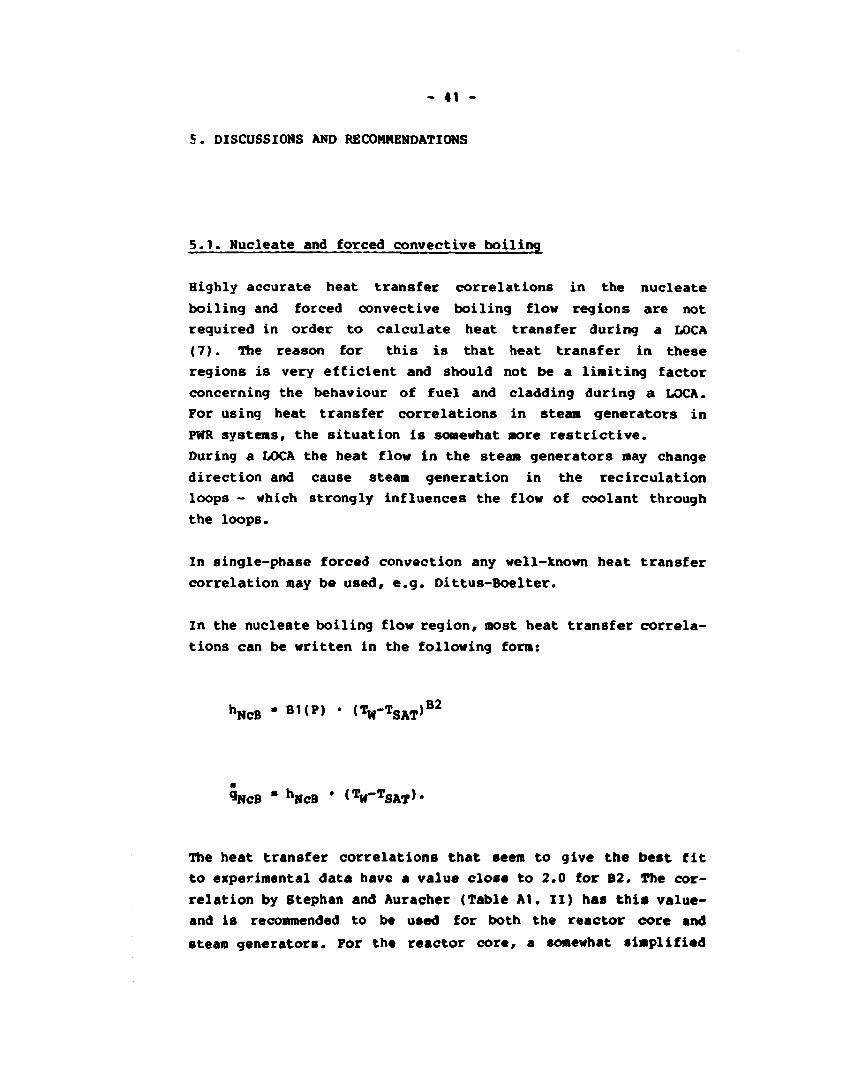
In the nucleate boiling flow region, most heat transfer correla
tions can be written in the following form:
h N c B - B1(P) • (TW-TSAT)B2
^NcB * hNcB ' t^tø-'sAT)'
The heat transfer correlations that seem to give the best fit
to experimental data have a value close to 2.0 for B2. The cor
relation by Stephan and Auracher (Table A1. II) has this value-
and is recommended to be used for both the reactor core and
steam generators. For the reactor core, a somewhat simplified
- 42 -
version of the Chen correlation is considered accurate enough.
5.2. Critical heat flu«
The results of the literature search are given in Appendix A2
and the outcome of some recent assessments of CHF correlations
in rod bundle geometries is summarized in Appendix B4.1.
Leung(22) has demonstrated that an appropriate steady state CHP
correlation was adequate for the prediction of CHP onset during
a wide range of transients. He also indicated that the local
condition hypothesis can be used for CHF predictions. This
method is most advantageous in transient analyses. It is very
difficult to define an adequate boiling length at each instance
during the course of a transient, which is a requirement when
other methods are employed.
In Appendix A2 it is recommended to use Griffith-Zuber correla
tion for the low mass flux range:
-240 < 6 < 100 kg/*2s.
Outside this mass flux range the Biasi and CISB-4 correlations
were found to be equally good possibilities. However, it has to
be emphasized that this outcome was based on the comparison
between the measured and predicted time to CHF during different
kinds of transient in round-tube or scaled-rod bundle test sec
tions. When Biasi and CISB-4 correlations were used for predic
tion of the CHF in full-scale rod bundle steady-state experi
ments they were found to be very non-conservative (cf. Appendix
B4.1). This was attributed to the development of these two
correlations from single-tube data. There were no provisions
for incorporating the effects of unheated wall surfaces and
internal rod-to-rod power distributions. As would be expected,
the rod bundle CHF correlations were found to be much more
accurate when predicting the CHF in this type of geometry, and
it was recommended that the Becker rod bundle CHF correlation

- 43 -
be used within the following parameter ranges:
Pressure 3.0 - 9.0 MPa
Mass flux 400 - 3000 kg/m2s
Heat flux 0.5 - 3.0 MW/m2
For mass fluxes between 100 and 400 kg/m2s an interpolation of
the Becker and the Griffith-Zuber correlations has to be made.
Above 9.0 MPa it is not clear which correlation to use. No
testing of CHF correlations in this pressure range has been
performed within the project, and no firm recommendation can
be given. In the literature several possible correlations
are reported, e.g. the correlation proposed by EPRI (8) and
the one by Bezrukov et al. (9), but these have to be more
thoroughly tested and validated before drawing any conclusions.
Also, the situation in the low-pressure range (P < 3.0 MPa) is
not very well examined. Due to the lack of rod bundle experi
mental CHF data for these low pressures no assessments of CHF
correlations have been made and thus no recommendations can be
given. It is obvious that there is a strong need for more
experimental data and analysis in this low-pressure range.
5.3. Transition boiling
The experimental data used in this comparison are primarily in
the vapour continuous flow region and only very few in the tran
sition flow between vapour and liquid continuous (churn/slug
flow).
The correlations selected for comparison (except the correlation
by Hsu) were developed primarily for the dispersed flow region
in vapour continuous flow. It cannot be expected that the cor
relations can be used in the inverted annular flow region, i.e.
44 -
liquid continuous flow.
The comparison shows the necessity of taking thermodynamic non-
equilibrium into account.
The comparison also shows that the direct liquid-wall contact
heat transfer is important and has to be accounted for espe
cially in regions near the CHF location. This is in contra
diction to the widely used assumption that the contact heat
transfer is negligible.
Much more work is needed, however, before transport phenomena
in transition boiling can be described.
It is the purely empirical and simple heat transfer correlation
by Bjornard and Griffith (11) that relates the test data best;
therefore, it must be recommended for use until better phenora-
enological correlations or models are developed.
The inverted annular flow region in liquid continuous flow has
not been examined.
5.4. Rewetting
The rewetting process means a reversal from film boiling condi
tions after DO or DNB back to nucleate boiling and the main
interest concerning the phenomena is connected with large LOCA
reflooding or spray cooling.
Two possible methods may be seen for the modelling of the rewet
ting front:
The two-dimensional heat conduction equation may be solved nu
merically and the moving mesh techniques are used to split the
heat structure around the rewetting front into finer meshes. The
numerical inaccuracy is avoided if the finest meshes in axial di
rection are shorter than 0.001 mm. In moving-mesh techniques the
heat transfer correlations are used for the nucleate boiling,

- 45 -
critical heat flux and transition boiling. The moving-mesh techniques should not be used if the computing time consumption is limited.
The second possibility is to apply a mathematical correlation for the revetting velocity. Then the formula of Dua and Tien is recommended :
0.5
Pe Bi / n aåt Bi \
• II + 0.40 • \ ew.(ew-i) ^ ew.(ew-ny
6»p»C»u h»6 T-TSAT Pe = ;fli • ; e » ; ew » S(TW)
k k T0-TSAT
The fitting parameters of the mathematical formula are the heat transfer coefficient h in the Biot, number Bi and the revetting temperature T0 in the nondimensional temperature. The recommended heat transfer coefficient is the critical heat flux of Zuber correlation divided by the temperature difference l&TsKT * TCHF~TSAT)* this difference is calculated from the wall temperature during nucleate boiling determined by the Chen correlation. The slowing down of the rewetting due to void fraction is taken into account by the factor (1-a) proposed by Griffith. Two possibilities are recommended for the rewetting temperature: the use of minimum film boiling temperature or a simpler formula like: TQ - TSAT + 160 + 6*ATgub .
5.5. Film boiling
The film boiling region can be divided into basically two flow
sub-regions: inverted annular flow and dispersed droplet flow.
The development of these sub-regions is strongly influenced by
the prevailing pre-CHP region which can be determined from a
flow region map.
For the inverted annular flow the heat transfer mechanisms are as yet not very well understood. Until more research sheds light on these issues a simplified approach using a modified Bromley correlation is recommended to calculate the wall heat transfer:
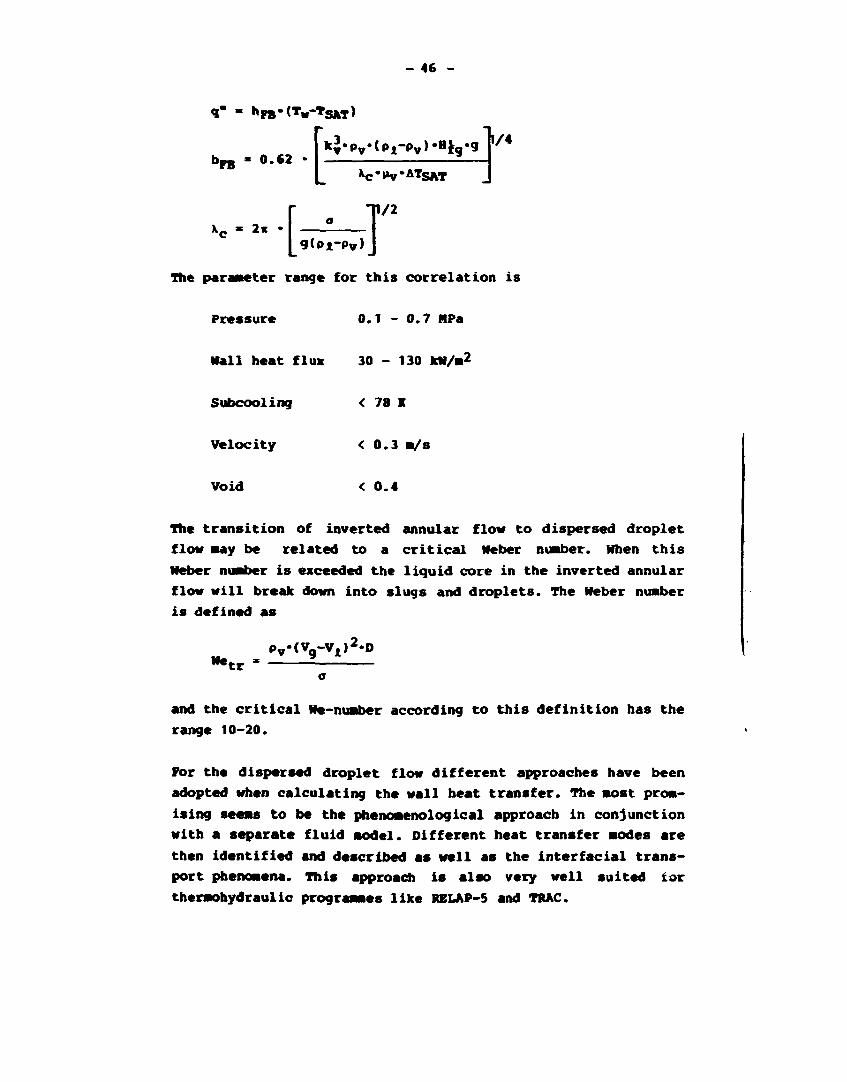
- 46 -
hre*tTw-*sjtt>
I«/« hre - o 62
k*'pv'(p*~pv)'li*9'q
L xc*»hr*ATSAT
Vc - 2* |_g(Pi-pv)J
The parameter range for this correlation is
Pressure 0.1 - 0.7 HPa
Wall heat flux 30 - 130 Ml/a?
Subcooling < 78 I
Velocity < 0.3 a/s
Void < 0.4
The transition of inverted annular flow to dispersed droplet
flow aay be related to a critical Neber nuaber. When this
Neber nuaber is exceeded the liquid core in the inverted annular
flow will break down into slugs and droplets. The Neber nuaber
is defined as
Netr Pv-<VVA,2,D
and the critical We-nuaber according to this definition has the
range 10-20.
For the dispersed droplet flow different approaches have been
adopted when calculating the wall heat transfer. The aost prom
ising seeas to be the phenoaenological approach in conjunction
with a separate fluid aodel. Different heat transfer aodes are
then identified and described as well as the interfacial transport phenomena. This approach is also very well suited tor
theraohydraulic prograaaes like RELAP-5 and TRAC.

- 47 -
In the film boiling region it is usually assumed- that the radiation and wall-to-liquid heat transfer terms are negligible compared with the wall-to-vapour terms. This latter heat transfer can be calculated according to the revised version of the modified CSO (Chen-Sundaram-Ozkaynak) correlation:
q" =• h-(Tw-Tw)
h * hmod CSO (1+Fs)<1+0«*/(L/D))
Fs - 250 p
* c
0.69 "l-XA
XA L J
0.49 Re"0-55
"mod CSO » --Cpvf*G-XA'Pr;2/3
f • V
-0.1
1 I 2e 9. _ * 3.48 - 4-log10| — + -L D Re v /lo-J
The basic interfacial processes are dealt with in Chapter 5.6.
When the flow region is single-phase steam flow, where the steam may be superheated, the well-proven correlations of Dittus-Boelter's type can be used to calculate the heat transfer coefficient. The Sieder-Tate correlation is one example of this type:
q" « h»(Tw-Tv)
. Re0-8.PrV3.f2l\ » ^w/
0.14
The revised version of the modified CSO correlation seems to have a smooth transition to this correlation when XA approaches unity.
- 48 -
For very low flows natural convection nay become a significant
contributor to the total heat transfer. For turbulent natural
convection heat transfer to single-phase vapour the following
correlation can be used:
q" = h»(Tw-Tw)
h = 0.13.kvf - ^ VI- Pr vp ^vf
where the properties are evaluated at film temperature.
5.6. Interfacial heat transfer
When thermodynamic nonequilibrium between the phases is assumed,
a constitutive model is needed for the interfacial heat transfer.
The way in which the constitutive model is applied depends on the
assumptions made in the hydraulic model. When a two-fluid model
is applied two constitutive equations are needed, one for the
heat transfer from the interface-to-vapour phase (Qig) and an
other from the interface-to-liquid phase (Qu). These are re
lated to the interfacial mass transfer as
Qig+QiJl
r » Hfg
where Hfg is the latent heat of evaporation.
If simplifying assumptions have been made in the hydraulics the
number of interfacial constitutive equations decreases. The u-
sual assumption is that one of the phases is saturated while the
other phase is in thermodynamic nonequilibrium. In that case only
one equation for the interfacial energy transfer must be speci
fied. Usually the model is applied for r. Because there is a
lack of experimental correlations the same approach is very
often used also with the two-fluid model. The interfacial heat
transfer rates are expressed ass
Qik ' hik#<TsAT-Tk>
- 49 -
where T is temperature, h ^ is a kind of heat transfer coef
ficient (Joule/m3*s*°C) and the subscript k is either g or A .
When this equation is used the phase can be forced to be satu
rated by applying a large interfacial heat transfer coefficient
hjjc. In some cases the interfacial heat transfer is closely
related to the wall heat transfer. One example is subcooled
boiling. In this case a separate wall boiling model must be
applied, because when the average fluid is subcooled, no eva
poration is predicted through the above equations. If rw is
the amount of wall flashing, the total flashing rate is expres
sed as:
rtot - rw + r
where f is calculated from the above mentioned equation, r is
negative (condensation) in the case of subcooled boiling. In
practice it is very difficult to model rw so that the total
flashing rate is correct. For example, the TRAC(PF1)-programme
was unable to predict any subcooled boiling in the test cases
analyzed in the SAK-5 project.
Another case where the interfacial heat transfer rate has a
strong effect on the wall heat transfer is post-dryout heat
transfer. In the post-dryout flow region the interfacial area
between the phases is small and the heat transfer coefficient
hig is low. Consequently, the vapour temperature is increasing
in that region, which results in higher wall surface tempera
tures if the wall heat transfer coefficient remains constant.
Encouraging results have been obtained in the SAK-5 project
by applying interfacial heat transfer models in the post-dryout
region. Another approach in the post-dryout region would be the
modification of the wall heat transfer coefficient so that
better agreement with experimental surface temperature is ob
tained. In fact, this is the only way if equilibrium between
the phases is assumed. The use of a nonequilibrium assumption
enables the more realistic prediction of the wall temperature
distributions.

50 -
Although the interfacial heat transfer has an important role in
two-phase flow predictions, relatively few empirical correla
tions exist at present. In the SAK-5 project only two areas
have been studied and only preliminary results have been ob
tained. These results cover the area of flashing and post-dryout
flow region.
The flashing rate is important in the prediction of the pressure
recovery following a rapid depressurization and in the predic
tion of the liquid superheat in quasi-steady flow. The latter
is important in the calculation of critical flow. Several
flashing correlations have been tested (14). According to
the test cases performed the experimental correlation of Bauer
et al. (15) gave the best agreement with experimental data.
This correlation can be expressed for h^x as
(1-o )*pf Cpx
»il " " t
where a is void fraction, Cp is specific heat and p* is liquid
density. The time constant i is defined as
660
(a+a0)(u+u0)* /T
where u is liquid velocity and P is pressure in Pa. This cor
relation is valid in the range of 0.01 < a < 0.96 and 5 m/s <
u < 54 m/s, when <x0 • UQ * 0. However, because there are
no other suitable correlations, it is suggested that this
correlation is extrapolated outside its validity limits. For
this purpose the constants aQ and u0 have been determined
to be 0.003 and 4 m/s. In this form the correlation predicts
critical flow data with good agreement. In the prediction of
the pressure recovery following a rapid depressurization, the
agreement seems to depend on the flow area. Relatively good
pressure history is predicted with medium-size pipes. In the
case of Edward's pipe test, the predicted pressure recovery
is too slow and in the case of a large vessel it is too fast.
However, this kind of uncertainty has not such a vital impor
tance as has the uncertainty in the calculated critical flow.
- 51 -
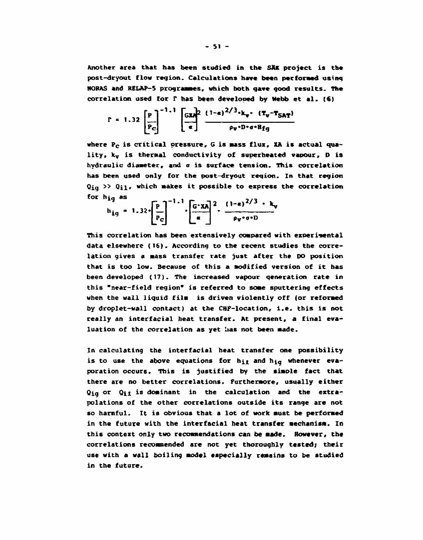
Another area that has been studied in the SAK project is the
post-dryout flow region. Calculations have been performed using
MORAS and RELAP-5 programmes, which both gave good results. The
correlation used for r has been developed by Webb et al. (6)
r = 1.32 i ] 1 " 1 H 2 <1~*)2/3*k** (Tv"TSAT>
where Pc is critical pressure, G is aass flux, XA is actual qua
lity, kv is thermal conductivity of superheated vapour, D is
hydraulic diaaeter, and a is surface tension. This correlation has been used only for the post-dryout reqion. In that region
Qig >> Qil» which makes it possible to express the correlation
for hig as
* • -M' -M pv«0*D
This correlation has been extensively compared with experimental
data elsewhere (16). According to the recent studies the corre
lation gives a mass transfer rate just after the DO position
that is too low. Because of this a modified version of it has
been developed (17). The increased vapour generation rate in
this "near-field region" is referred to some sputtering effects
when the wall liquid film is driven violently off (or reformed
by droplet-wall contact) at the CHP-location, i.e. this is not
really an interfacial heat transfer. At present, a final eva
luation of the correlation as yet has not been made.
In calculating the interfacial heat transfer one possibility
is to use the above equations for h u and hig whenever eva
poration occurs. This is justified by the simple fact that
there are no better correlations. Furthermore, usually either
Qig or Qix is dominant in the calculation and the extra
polations of the other correlations outside its range are not
so harmful. It is obvious that a lot of work must be performed
in the future with the interfacial heat transfer mechanism. In
this context only two recommendations can be made. However, the
correlations recommended are not yet thoroughly tested; their
use with a wall boiling model especially remains to be studied
in the future.
- 52 -
6. CONCLUSION
It is both natural and rather obvious to test heat transfer
correlations in the environment in which they are to be used,
i.e. the computer programmes TRAC, RELAP-5 and NORA. The
advantage is that parameters not measured in the experiment
are calculated under conditions in the programme which ought
to correspond to reality in the experiment.
It was, however, not possible in the transient calculations to
assess the adequacy of the heat transfer package in the indi
vidual programmes. It can not be excluded that other transport
phenomena (subcooled void, slip, thermodynamic nonequilibrium)
and empirical correlations veil the actual aim, viz. to
assess the heat transfer correlations.
The general idea, to use the computer programmes in the com
parison, was retained, but it was decided to make a switch in
the selection of experiments from transient to steady state,
simple experiments.
The accuracy of heat transfer correlations in pre-CHF regions
i.e. the nucleate boiling region and the forced convective
boiling region does not have to be very high for the purpose
of calculating heat transfer during a LOCA The heat transfer
in these regions is very efficient and should not be a limit
ing factor for the fuel and cladding during a LOCA.
The critical heat flux (CHF) calculations were carried out
with the W-3 correlation (4) (primarily a DNB correlation)
in RELAP-5 as well as the Biasi correlation (5). The pre
dicted dryout locations were too far upstream (up to ~ 3 m
at low pressure). The CHF were in some cases determined by a
cutoff void limit of 0.96 when the Biasi correlation was
used.
- 53 -
The results from TRAC were fairly accurate except at low pres
sure. TRAC makes use of the Biasi correlation, but in none of
the cases did the correlation determine the locus of dryout.
An arbitrarily chosen cutoff void limit of 0.97 caused dryout.
The NORAS calculations used three different CHF-correlations,
Biasi, CISB-4 (24) and Becker (64). Biasi and Becker corre
lations predicted dryout too far downstream while CISE-4 corre
lation predicted dryout too far upstream at high quality and
too far downstream at low quality.
It was therefore necessary to freeze the locus of CHF at the
measured location in order to compare the surface temperatures.
This comparison was not good in any of the programmes used.
The calculated surface temperatures were too low in RELAP-5
and TRAC indicated an interfacial heat transfer that was too
high. NORAS gave too high surface temperatures,i.e. too low
interfacial heat transfer.
This can be seen from a single calculation using NORAS and 5
calculations using RELAP-5 in Figs. B2.21-B2.27. In two
of the RELAP-5 cases the interfacial heat transfer was so
high that no vapour superheat was calculated (the liquid and
vapour post-dryout temperatures were about the same).
The test section was an electrically heated tube with a very
low thermal capacity i.e. a typically heat flux controlled
experiment. The thermodynamic nonequilibrium effects are
therefore primarily governed by mass transfer between droplets
and vapour due to interfacial heat transfer. A decrease in
the vapour generation rate will increase the vapour tempera
ture under equal conditions, thus allowing the thermodynamic
nonequilibrium to be more pronounced.
The programmes were modified by implementing a recently deve
loped vapour-generation model by Chen (6). Recalculated re
sults were substantially improved and a satisfactory agree
ment between measured and calculated post-dryout surface tem
peratures was obtained.

- 54 -
Prom these examinations, together with the examinations of the
transition boiling heat transfer with a separate computer pro
gramme, it is obvious that more realistic and phenomenological
heat transfer models have to be developed. It must be recognized
that the degree of thermodynamic nonequilibrium at any axial lo
cation is dependent not only on local conditions but especially
on the upstream competition between the heat transfer mechanisms
wall-to-vapour, wall-to-droplet and vapour-to-droplet.
Up to now this report treated the post-CHF region in more
independent chapters, transition boiling heat transfer, revett
ing, interfacial heat transfer and film boiling with and with
out droplets. To get realistic models the transport phenomena
have to be considered in more detail and the post-dryout region
may be treated as one region where the dividing point between
transition boiling and film boiling is not the minimum film
boiling temperature, but rather the point where the droplet can
wet the surface or not. The surface can/in fact/ be rewetted
even if the minimum film boiling temperature has been passed,
if the momentum of the droplets perpendicular to the surface can
prevail over the repulsive forces due to evaporation at the wall.
The project decided to touch upon these phenomena in a some
what more detail and the results are discussed in Appendix C.
With respect to the discouraging results of critical heat
flux calculations, the project decided to make a closer elabora
tion of 4 relevant CHF-correlations: Barnett, Becker, CISE-4 and
Bias! using results from full-scale rod bundle experiments.
The results indicate that Biasi and CISE-4 correlations, which
are used in computer programmes like RELAP-5 and TRAC, cannot
predict the CHF-conditions with adequate accuracy. An explana
tion is believed to be that these two correlations are developed
from single tube data and have no provisions to incorporate
the influence of unheated surfaces and internal rod-to-rod
power distribution. The two other CHF-correlations are de
veloped for rod bundle geometries and correlate the experimental
data more accurately. It is therefore recommended that these
correlations instead of Biasi and CISE be used.
- 55 -
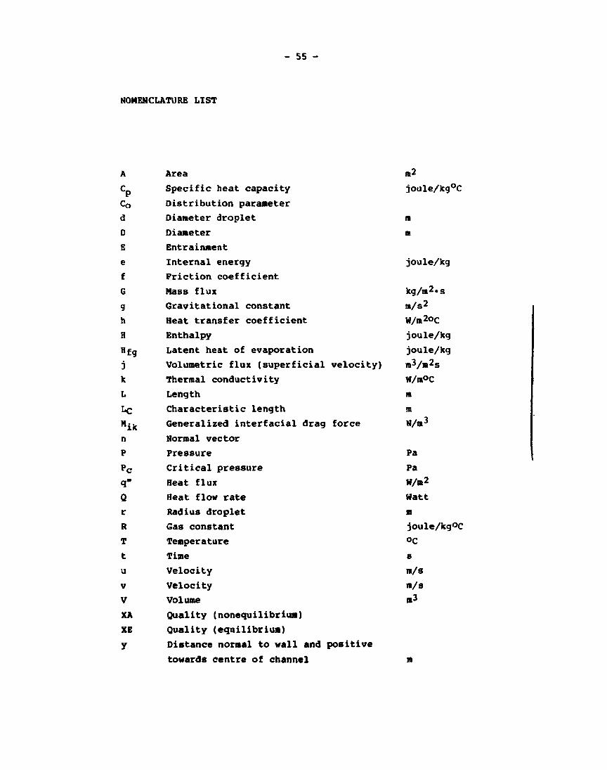
NOMENCLATURE LIST
A
CP Co d D
E e f
G
g h H
Hfg
j k
L
tc Mik n P
Pc q" Q r R
T
t
u
V
V
XA
XE
y
Area
Specific heat capacity
Distribution parameter
Diameter droplet
Diameter
Bntrainment
Internal energy
Priction coefficient
Mass flux
Gravitational constant
Heat transfer coefficient
Enthalpy
Latent heat of evaporation
Volumetric flux (superficial velocity)
Thermal conductivity
Length
Characteristic length
Generalized interfacial drag force
Normal vector
Pressure
Critical pressure
Heat flux
Heat flow rate
Radius droplet
Gas constant
Temperature
Time
Velocity
Velocity
Volume
Quality (nonequilibrium)
Quality (equilibrium)
Distance normal to wall and positive
towards centre of channel
*2
joule/kg°C
m
m
joule/kg
kg/m2«s
m/S2
W/m2oc
joule/kg
joule/kg
iB^/m2s
W/ra°C
m
m N/m3
Pa
Pa W/m2
Watt
m joule/kgOC
c-C
s m/s
m/s m3
m
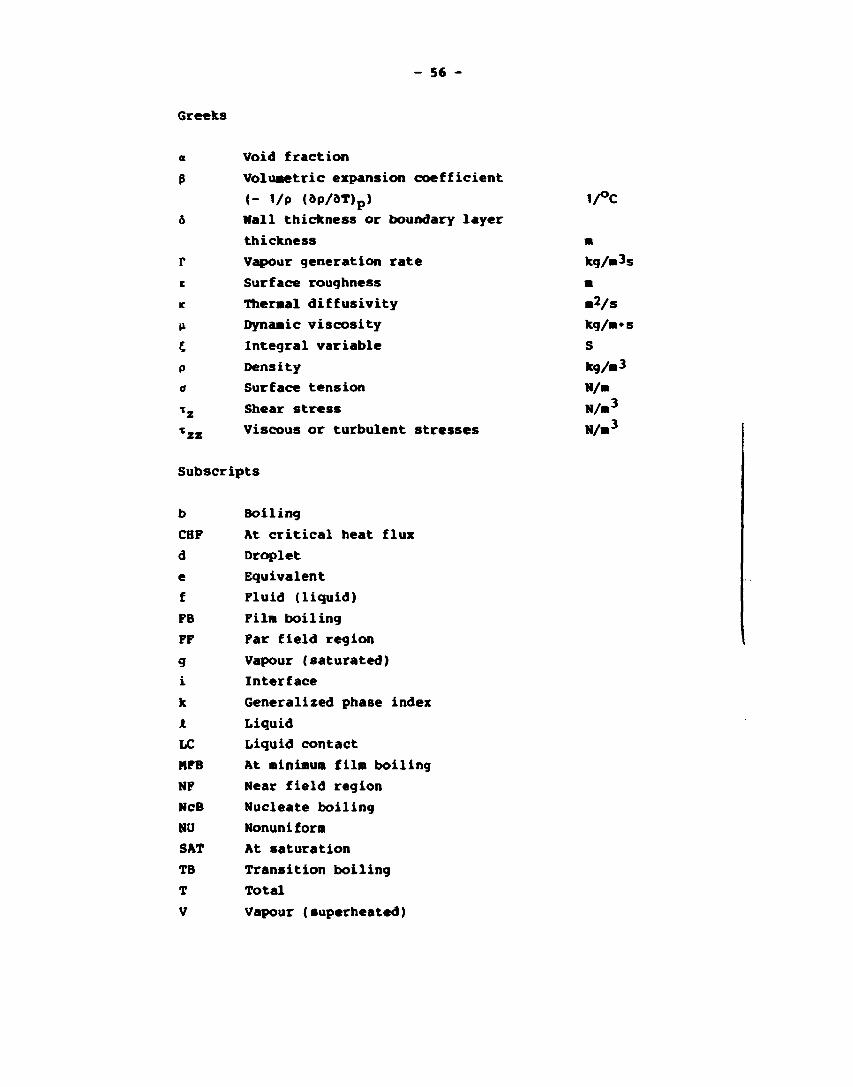
- 56 -
Greeks
a Void fraction
p Voluaetric expansion coefficient
(- 1/P (aP/5T)p) 1/°C 6 Hall thickness or boundary layer
thickness a r Vapour generation rate kg/a3s e Surface roughness a
r Theraal diffusivity a2/s ti Dynamic viscosity kg/a*s £ Integral variable S
p Density kg/a3 o Surface tension N/a
xz Shear stress N/a3
x z z Viscous or turbulent stresses N/a3
Subscripts
b Boiling
CHP At critical heat flux d Droplet
e Equivalent f Pluid (liquid)
FB Film boiling FP Far field region
g Vapour (saturated) i Interface
k Generalized phase index
X Liquid LC Liquid contact HFB At minimum film boiling
NF Near field region NcB Nucleate boiling
NU Nonuniform SAT At saturation
TB Transition boiling T Total
V Vapour (superheated)
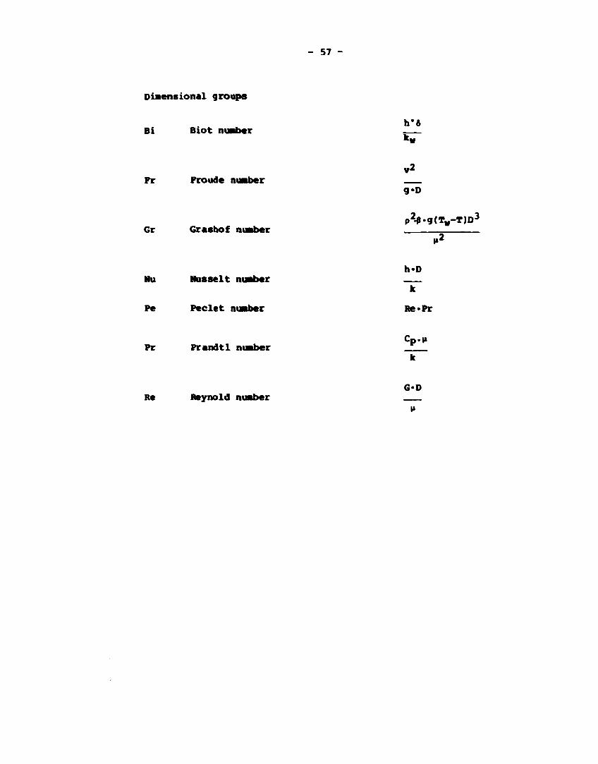
- 57 -
Disensional groups
Bi Biot nuaber
Pr Froude nuaber
Gr Grashof nuaber
Nu Musselt nuaber
Pr Prandtl nuaber
Re Reynold nuaber
h*6
v2
g.D
p2-P«g(Tw-T)D3
h-D
Pe Peclet nuaber Re*Pr
G«D
- 58 -
REFERENCES.
1 . Y. Y. HSU Best-Estimate Recommendations for Blowdown Heat Transfer. LOCA Research Highlights, 1975 (NRC).
2. K. M. BECKER et al. An Experimental Investigation of Post Dryout Heat Transfer KTH-NEL-33 Department of Nuclear Reactor Engineering, Royal Institute of Technology, Stockholm, May 1983
3. J. C. CHEN Correlation for Boiling Heat Transfer to Saturated Fluids in Convective Flow I&EC Process Design and Development. Vol 5, No 3 July 1966
4. L. S. TONG Prediction of Departure from Nucleate Boiling for an Axially Non-uniform Heat Flux Distribution. Journal of Nuclear Energy, 21, pp 241-248
5. L. BIASI et al. Studies on Burnout Part 3 Energia Nucleare 14, 1967
6. S. H. WEBB, J. C. CHEN, R. K. SUNDARAM. Vapour Generation Rate in Non-equilibrium Convective Film Boiling. 7th Int Heat Transfer Conference, Munich, Sept 1982
7. J. RASMUSSEN Correlations for Heat Transfer in Forced Convection and Nucleate Boiling and Critical Heat Flux. SAK-5-N (81)-2.
8. D. G. REDDY, C. F. FIGHETTI. Parametric Study of CHF-data, vol. 2 A Generalized Subchannel CHF-correlation for PWR and BWR Fuel Assemblies. EPRI NP-2609. Jan. 1983.
9. YU. A. BBZRUKOV et al. Experimental Investigation and Statistical Analysis of Data on Burnout in Rod Bundles for Water-Moderated Water-Cooled Reactors. Teploenegetika, 1976, 23(2) 80-82.
- 59 -
10. J. G. M. ANDERSEN et al. BWR Refill-Reflood Program Basic Models for the BWR Version of TRAC NUREC/CR 2573 (GEAP-22051) September 1983.
11. T. A. BJORNARD and P. GRIFFITH PWR Blowdown Heat Transfer. Thermal and Hydraulic Aspects of Nuclear Reactor Safety. Vol. I LWR. ASHE Winter Annual Meeting Atlanta, Georgia, 1977
12. A. SJOBERG "Heat Transfer in the Post Critical Heat Flux Regime" Studsvik Technical Report NR-82/77 SAK-5-S(82)l Jan 1982
13. K. MISHIMA, M. ISHII "Flow Regime Transition Criteria for Upward Two-Phase Flow in Vertical Tubes" Int. J. of Heat and Mass Transfer, Vol. 27, No 5 May 1984
14. T. SIIKONEN Comparison of Flashing Heat Transfer Correlations Second International Topical Meeting on Nuclear Reactor Thermal-Hydraulics, Santa Barbara, Jan. 11-14, 1983.
15. E. G. BAUER, G. R. HOUDAYER, H. M. SMEAN A Non-equilibrium Axial Plow Model and Application to Loss-of-Coolant Accident Analysis: The CLYSTERE System Code CSNI Specialist Meeting on Transient Two-Phase Plow, Toronto 1976.
16. R. C. GOTTULA, R. A. NELSON, J. C. CHBN, S. NETI R. K. SUNDARAM. Forced Convective Nonequilibrium Post-CHF Heat Transfer Experiments in a Vertical Tube ASME-JSME Thermal Engineering Joint Conference, Honolulu, March 20-24, 1983.
17. S. W. WEBB, J. C. CHEN A Two-Region Vapor Generation Rate Model for Convective Film Boiling International Workshop on Fundamental Aspects of Post-Dryout Heat Transfer, Salt Lake City, April 1-4, 1984.

- e o -
is. P. CAMPOLOMGHI et al. Subcooled and Bulk Boiling Correlations for Thermal Design of Steaa Generators. Advances in Heat Transfer CNBN-RT/ING (80)22.
19. K. STEPHAN, H. AORACHBR Correlations for Nucleate Boiling Heat Transfer in Forced Covection. Int. J. of Heat and Mass Transfer, Jan. 1981.
20. J. G. COLLIER Convective Boiling and Condensation McGraw-Hill, London, 1972.
21. G. P. HEWITT Critical Heat Plus in Plow Boiling 6th Intern. Heat Transfer Conf. Toronto, 1978.
22. J. C. LEUNG Transient Critical Heat Plus and Blowdown Heat Transfer Studies. ANL-80-53, Argonne, Illinois.
23. M. COHO et al On the Liaiting Critical Quality and the "deposition controlled" Burn-Out. CN£N-RT/ING(80)22.
24. A. BRA, G. P. GASPARI Heat Transfer Data in the Liquid Deficient Region for Steam-Water Mixtures at 70 kg/cm2 in Tubular and Annular Conduits. CISB-R 184, 1966.
25. K. H. BECKER, D. H. LING Burnout Measurements in a Round Tube of 7.1 » Heated Length KTH, Stockholm, 1970
2 6 . H. ABEL-LARSBN. Comparison between 5 Transistion Boiling Heat Transfer Correlations and some Temperature Controlled Test-Data at 1-4 bar (BPRI) SAK-5-D(84)-2
27. H. ABEL-LARSBN. Heat Transfer in the Transition Boiling Region SAK-5-D(81)-2.
- 61 -
28. D. C. GROENVBLD. Heat Transfer Phenomena Related to the Boiling Crisis AECL-7239, March 1981
29. J. C. CHEN et al. A Phenomenological Correlation for Post-CHF Heat Transfer. NUREG-0237, June 1977
30. O. C. ILOEJE et al. Three-Step Model of Dispersed Flow Heat Transfer (Post-CHF Vertical Plow). ASME Winter Annual Meeting 1975, 75-WA/HT-l.
31. L. S. TONG and J. D. YOUNG. A Phenomenological Transition and Film Boiling Heat Transfer Correlation 5.Int.Heat Transfer Conf., Sept. 1974. (Paper B3.9)
32. Y.Y. HSU Tentative Correlations of Reflood Heat Transfer. LOCA Research Highlights, 1975, (NCR).
33. TROND A. BJORNARD and PETER GRIPFITH. PWR Blow-Down Heat Transfer. ASME Winter Annual Meeting, Vol.1, 1977.
34. KIRCHNER, WALTER and PETER GRIFFITH Reflood Heat Transfer in a Light Water Reactor. AICHE-Symp. Series 1977: 73 NO. 164.
35. J. MIETTINEN. The Modelling of the Transition Boiling During Rewetting of a Hot Surface With an Analytical Correlation. SAK-5-F(82)2
36. J.G.M. ANDERSEN. Low-Plow Film Boiling Heat Transfer on Vertical Surfaces. PART I. 16. Nat. Heat Transfer Conf., AICHB-52, St. Louis, 1976.
37. J.E. LEONHARD, K.H. SUN and G.E. DIX Low-Plow Film Boiling Heat Transfer on Vertical Surfaces. PART II. Same Conf.
38. M.K. DENHAM Inverted Annular Film Boiling and the Bromley Model AEEW-R 1590 ABB, Winfrith, Dorchester Jan, 1983.

- 62 -
39. S.M. NIJHAWAN Experimental Investigation of Thermal Nonequilibrium in Post-Dryout Steam-water Flow Ph.D. Dissertation, Lehigh University, 1980
40. S. M. NIJHAWAN et al Measurement of Vapour Superheat in Post-Critical Heat-Flux Boiling Journal of Heat Transfer Vol 102 Aug 1980
41. D. G. EVANS, S. W. WEBB, J. C. CHEN Measurement of Axially Varying Nonequilibrium in Post-Critical-Heat-Flux Boiling in a Vertical Tube NUREG/CR-3363, Vols 1 and 2 June 1983
42. R. C. GOTTULA et al Forced Convective, Nonequilibrium Post-CHF Heat Transfer Experiment Data and Correlation Comparision Report NUREG/CR-3193, EGG-2245 DRAFT Jan 1984
43. J. C. CHEN Review of Post-Dryout Heat Transfer in Dispersed Two-Phase Flow Lehigh University, PA Presented at the International Workshop on Fundamentals Aspects of Post-Dryout Heat Transfer Salt Lake City, April 1984
44. V. H. RANSOM et al RELAP5/M0D1 Code Manual Volume 1 System Models and Numerical Methods NUREG/CR-1826. EGG-2070 March 1982
45. A. SJOBERG RELAP5/M0D1 Calculations on Five Steady State Post-Dryout Heat Transfer Experiments STUDSVIK Technical Report NR-83/338 SAK-5-S(83)2 Dec 1983

- 63 -
46. J. RASMUSSEN Simulation of Non-Equilibrium Effects State Post-Dryout Heat Transfer IFE Report IPE/KR/P-84/069 SAK-5-N(84)1 June 1984
47. A. SJOBERG "RELAP5/M0D1 Simulation of Non-Equilibrium Effects in the Post-Dryout Regime STUDSVIK Technical Report NR-84/452 SAK~5-S(84)1 Aug 1984
48. K. G. CONDIE et al Forced Convective, Nonequilibrium Post-CHF Heat Transfer Experiment: Description, Data Analysis and Correlation Comparison Presented at the International Workshop on Fundamental Aspects of Post-Dryout Heat Transfer Salt Lake City April 1984
49. T. SIIKONEN Calculations on some Steady-State Heat Transfer Experiments, (to be published)
50. T. SIIKONEN Comparison of Plashing Heat Transfer Correlations Second International Topical Meeting on Nuclear Reactor Thermal-Hydraulics, Santa Barbara Jan. 11-14, 1983
51. A. R. EDWARDS, T. P. 0'BRIAN Studies of Phenomena Connected with the Depressurization of Water Reactors J. of the British Nuclear Society Vol. 9, No. 2, 1970
52. The Marviken Full Scale Critical Flow Tests Results from Test 15 MXC-215, Sept. 1979
53. L. R. KEVORKOV, S. Z. LUTONINOV, L. K. TIKHONENKO Influence of the Scale Factors on the Critical Disharge of Saturated Water from Straight Tubes with Sharp Inlet Edge. Teploenergetika 24(7), 1977.

- 64 -
54. Ph. VERNIER, Ph. BERNE An Appraisal of Interfacial Vapor Generation Laws Used in Thermalhydraulics Analysis, Second International Topical Meeting on Nuclear Reactor Thermalhydraulics, Santa Barbara Jan. 11-14, 1983.
55. P. SAHA, B. S. SHIRALKAR, G. E. DIX A Post-Dryout Heat Transfer Model based on Actual Vapour Generation Rate in Dispersed Droplet Regime ASME Paper 77-HT-80, 1977.
56. R. ROUMY Burn out in Transient Conditions on Circular Tubes Presented at European Two Phase Plow Meeting Harwell, June 1974
57. T. SIIKONEN, H. OLLIKKALA RELAP5 Calculations for a Nucleate Boiling and CHF Test Case VTT Technical Report SAK-5-P(82)4
58. R. A. SMITH, P. GRIPPITH A Simple Model for Estimating Time to CHP in a PWR LOCA ASME paper No 76-HT-9, 1976
59. H. N. GUERRERO et al Single Tube and Rod Bundle Blowdown Heat Transfer Experiments Simulating Pessurized Water Reactor LOCA Conditions ASME-76-HT-11
60. J. MIETTINEN, T. SIIKONEN Analysis of Steady Dryout Experiments (Becker) with RELAP5 VTT Technical Report OAP-22/83 SAK-5-F(83)2, Sep 1983
61. A. SJOBERG Analysis of Three Steady State DO Experiments with RELAP5/MOD1 Studsvik Technical Report NR-83/276 SAK-5-S(83)l, June 1983
62. H. ABEL-LARSEN, P. ASTRUP Analysis of 4 Steady State Critical Heat Flux Experiments (Becker) with TRAC-PP1, SAK-5-D(83)l May 1983
- 65 -
63. J. RASMUSSEN NORAS Calculations on soae Steady-State Heat Transfer Experiments with B O IFE Report IFE/KR/F-83/031 SAK-5-N(83)l June 1983
64. K. II. BECKER An Analytical and Experimental Study of Burnout Conditions in Vertical Round Ducts, Nucleonik 9, pp 257-270, 1967
65. T. VANTTOLA Testing of Wall Heat Transfer Package of RELAP5 Draft VTT Technical Report SXK-S-F(84)~ ? Sept 1984
66. J. HIETTINEN Comparisons of Heat Transfer Models in RELAP5/MOD1, DRDFAN and FLOT Draft VTT Technical Report SAK-5-F(84) Sept 1984
67. A. SJOBERG RELAP5/HOD1 Calculations on Five Steady State Post Dry-out Heat Transfer Experiments Studsvik Technical Report KR-83/338 SAK-5-S(83)2, Dec 1983
68. H. ABEL-LARSEN Analysis of 5 Steady State Critical Heat Flux Experiments (Becker) with Prozen CHF-Location using TRAC(PFl) SAK-5-D(83)-5 September 1983
69. A. SJOBERG RELAP5/MOD1 Simulation of Non-Equilibrium Effects in the Post-Dryout Regime Studsvik Technical Report NR-84/452 SAK-5-S(84)l. Aug 1984
70. J. RASMUSSEN NORAS- Calculations on Some Steady State Heat Transfer Experiments with BO Using a New Correlation for Vapour -Droplet Heat Transfer IFE Report IFE/KR/P-83/052 SAK-5-N(83)2, Aug 1983
- 66 -
71. J. RASMUSSEN Simulation of Non-Equilibrium Effects in Post-Dryout Heat Transfer IFE Report IFE/RR/F-84/069 SAK-5-N(84)l, June 1984
72. G. L. YODER et al Dispersed Flow Film Boiling in Rod Bundle Geometry - Steady State Heat Transfer Data and Correlation Comparisons, NUREG/CR-2435 ORNL-5822, March 1982
73. L. SARDH, K. M. BECKER Assessment of CHF Correlations Based on Full-Scale Rod Bundle Experiments Royal Institute of Technology, Nuclear Reactor Engineering KTH-NEL-36 Stockholm Oct. 1984
74. P.G. BARNETT A Correlation of Burn Data for Uniformly Heated Annuli and its Use for Predicting Burnout in Uniformly Heated Rod Bundles AEEW-E463 1966
75. K.M. BECKER A Burnout Correlation for Flow of Boiling Water in Vertical Rod Bundles AE-276, April 1967
76. G.P. GASPARI et al. A Rod Centered Subchannel Analysis with Turbulent Mixing for Critical Heat Flux Predictions in Rod Clusters Cooled by Boiling Water Proc of the 5th International Heat Transfer Conference Tokyo, Sept. 1974
77. DESIRELLO et al. Critical Power and Mass Content in a 8x8 Bundle Paper Presented at the European Two-Phase Flow Group Meeting in Eindhover, June, 1981
- 67 -
78. S. PIMPUTKAR M. GROSS The Thermal Hydraulic Performance of a 81-Rod Bundle under Boiling Hater Reactor Conditions Paper Presented at the European Two-Phase Flow Group Meeting in Ispra, June, 1979.
79. L. NILSSON FIX-II Loca Blowdown and Pump Trip Heat Transfer Experiments STUDSVIK REPORT NR-83/274, 1983
80. 0. NYLUND et al. Hydrodynamic and Heat Transfer Measurements on a Full-Scale Simulated 36-Rod Marviken Fuel Element with Non-uniform Radial Heat Flux Distribution. PRIGG-3, 1970
81. 0. NYLUND et Hydrodynamic and Heat Transfer Measurements on a Full-Scale Simulated 36-Rod Bundle BHWR Fuel Element with Non-Uniform Axial and Radial Heat Flux Distribution. PRIGG-4, 1970
82. F. H B0WDITCH, R. T. SMYTH Dryout and Pressure Drop Experiments on a Simulated SGHWR Channel with Five Unheated Rods AEEW-M757, 1967
83. K. M. BECKER et al Measurements of Burnout Conditions in Vertical Round Tubes with Non-Uniform Axial Heat Flux AE-RL-1153, Nov 1969
84. K. M. BECKER Personal Communication Oct. 1984
85. 0. NYLUND et al OP-64. Results of BURNOUT Measurements ASEA-ATOM FRIGG PM-64 (ASEA-ATOM Proprietary) Jan 1970
- e s
se. A. SJOBERG, K. TANGEN Comparison between OF-64 Burnout-Data and Dryout-Locations Calculated from RELAP5 Fluid Conditions using Becker's CHF Correlation STUDSVIK Technical Report NR-84/473 Restricted Distribution SAK-5-S(84)2, 1984
87. J. WEISMAN et al Studies of Transition Boiling Heat Transfer with Saturated Water at 1-4 bar. EPRI-NP-1899, June, 1981.
88. H. ISHII, H.A. GROLHES Inception Criteria for Droplet Entrainment in Two-Phase Concurrent Film Flow. AIChE Journal, Vol.21, NO. 2, March 1975.
89. G. B. WALLIS One-dimensional Two-Phase Flow. McGraw-Hill Book Co., Inc., New York, 1969.
90. R. LEE et al Size and Number Density Change of Droplet Populations above a Quench Front during Reflood Int. Journ. Heat Mass Transfer Vol. 27, No., 4, pp. 573-585, 1984.
91. N. LEE et al PHR FLECHT SEASET Unblocked Bundle, Forced and Gravity Reflood Task Data Evaluation and Analysis Report. NUREG/CR-2256, EPRI NP-2013, WCAP-9891 Nov. 1981.
92. R.S. BRODKEY The Phenomena of Fluid Motions Addison-Wesley Publishing Co. Reading, Mass., USA.
93. M. ISHII "Thermo-Fluid Dynamic Theory of Two-Phase Flow". Eyrolles, Paris 1975.
94. S. BANERJEE, A. M. CHAN "Separatet Flow Models - I. Analysis of the Average and Local Instantaneous Formulations" Int. Journal of Multiphase Flow, Vol. 6 1980

- 69 -
95. G. YADIGARAGLU, T. T. LAHBY Jr. "On the Various Forms of the Conservation Equations in Two-Phase Flow" Int. Journal of Multiphase Flow, Vol. 2 1976.
96. N. ZUBER, J.A. FINDLAY "Average Volumetric Concentration in Two-Phase Plow Systems" Journal of Heat Transfer, Vol. 87 1965.
97. T. SAITO "Multi-Fluid Modeling of Two-Phase Flow and Heat Transfer: Application to Critical Heat Flux Prediction for BWR Conditions" Ph. D. THESIS, Nuclear Engineering University of Wisconsin - Madison 1977
98. M. ISHII, K. MISHIMA "Two-Fluid Model and Hydrodynamic Constitutive Relations" Nuclear Engineering and Design, 82 Dec. 1984
99. M. ISHII, K. MISHIMA "Study of Two-Fluid Model and Interfacial Area" ANL. NUREG/CR - 1873 Dec. 1980
100. M. ISHII, N. ZUBER "Drag Coefficient and Relative Velocity in Bubbly, Droplet or Particulate Plows" AIChE Journal, Vol. 25, No. 5 Sept. 1979
101. M. ISHII, T. C. CHAWLA "Local Drag Laws in Dispersed Two-Phase Plow" ANL-79-105, NUREG/CR-1230 Dec. 1979
102. R. T. LAHEY Jr. et al "The effect of Virtual Mass on the Numerical Stability of Accelerating Two-Phase Plows" Int. Journal of Multiphase Plow, Vol. 6 1980
103. H. LAMB "Hydrodynamics" Sixth Edition, pp. 123-124 Dover Publications New York 1932
- 70 -
104. N. ZUBER "On the Dispersed Two-Phase Plow in the Laminar Plow Regime" Chemical Engineering Science, Vol. 19. 1964
105. H. LAMB "Hydrodynamics" Sixth Edition, pp. 124-125 Dover Publications New York 1932
106. O. RATHMANN The Added Mass Force Dependence on Concentration by Numerical Solution" Risø Report NORHAV-D-80 May 1981
107 . E . N. GANlC, W. M. ROBSENOtf "On the Mechanism of Liquid Drop Deposition in Two-Phase Flow" ASMB Meeting, New York City, Dec. 1976
108. A.J. CLARE, S.A. PAIRBAIN Droplet Dynamic and Heat Transfer in Dispersed Two-Phase Flow, int. workshop on Fundamental Aspects of Post-Dryout Heat Transfer, Salt Lake City, 1984.
109. K.H. SUN, J.M. CONZALES Calculations of Combined Radiation and Convection Heat Transfer in Ros Bundles under Emergency Cooling Conditions, ASME, 75-HT-64.
110. A.P. VARONE, W.M. ROHSENOW Post-Dryout Heat Transfer Predictions, Int. Workshop on Fundamental Aspects of Post-Dryout Heat Transfer, Salt Lake City, 1984.

Dt2boool2> Nora
Heat Transfer Correlations in Nuclear Reactor Safety Calculations VW.I
RFA
CE
TE
MP
ER
AT
UR
E
-
CO
TMFB D
T fCHF
/ B
-""A
/ F
/
/ |E
/l / 1 / 1
/ 1 / !
/ i
f i i
V i X i
• > •
SURFACE HEAT FLUX
u ÉAiiattÉaii
fcflison cufiMiMltt lor yhdyiifci aomicantfgy
RIS0-M-25O4
6«. *).
HEAT TRANSFER CORRELATIONS IN
NUCLEAR REACTOR SAFETY CALCULATIONS
SAK-5
H. Abel-Larsen, Risø
A. J.
T.
J.
A.
K.
Olsen,
Miettinen,
Siikonen,
Rasmussen,
Sjdberg,
Becker,
Risø
VTT
VTT
I FE
Studsvik
KTH
June 1985
Risø: Risø National Laboratory, Denmark
VTT: Technical Research Centre of Finland
IFE: Institute for Energy Technology, Norway
Studsvik: Studsvik Energiteknik AB, Sweden
KTH: Royal Institute of Technology, Stockholm, Sweden
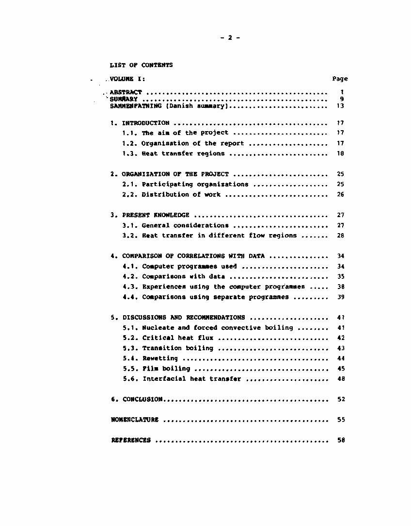
- 2 -
LIST OP CONTENTS
..VOLUME I: Page
. ABSTRACT 1 ' SUMMARY 9 SAMMENFATNING (Danish summary) 13
1. INTRODUCTION 17
1.1. The aim of the project 17
1.2. Organisation of the report 17
1.3. Heat transfer regions 18
2. ORGANIZATION OP THE PROJECT 25
2.1. Participating organizations 25
2.2. Distribution of work 26
3. PRESENT KNOWLEDGE 27
3.1. General considerations 27
3.2. Heat transfer in different flow regions 28
4. COMPARISON OP CORRELATIONS WITH DATA 34
4.1. Computer programmes used 34
4.2. Comparisons with data 35
4.3. Experiences using the computer programmes 38
4.4. Comparisons using separate programmes 39
5. DISCUSSIONS AND RECOMMENDATIONS 41
5.1. Nucleate and forced convective boiling 41
5.2. Critical heat flux 42
5.3. Transition boiling 43
5.4. Rewetting 44
5.5. Film boiling 45
5.6. Interfacial heat transfer 48
6. CONCLUSION 52
NOMENCLATURE 55
REFERENCES 58
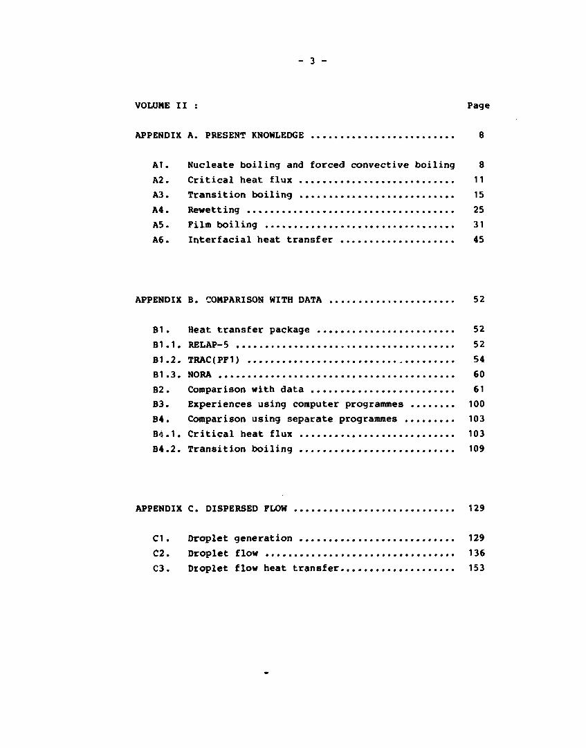
- 3 -
VOLUME II : Page
APPENDIX A. PRESENT KNOWLEDGE 8
Al. Nucleate boiling and forced convective boiling 8
A2. Critical heat flux 11
A3. Transition boiling 15
A4. Re wetting 25
A5. Film boiling 31
A6. Interfacial heat transfer 45
APPENDIX B. COMPARISON WITH DATA 52
B1. Heat transfer package 52
B1.1. RELAP-5 52
B1.2. TRAC(PP1) 54
B1.3. NORA 60
B2. Comparison with data 61
B3. Experiences using computer programmes 100
B4. Comparison using separate programmes 103
B4.1. Critical heat flux 103
B4.2. Transition boiling 109
APPENDIX C. DISPERSED FLOW 129
CI. Droplet generation 129
C2. Droplet flow 136
C3. Droplet flow heat transfer 153
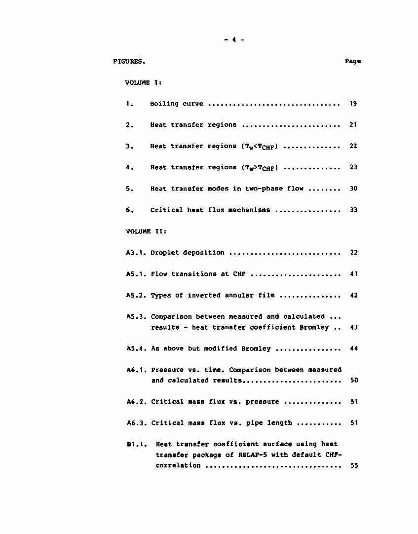
- 4 -
FIGURES. Page
VOLUME I:
1. Boiling curve 19
2. Heat transfer regions 21
3. Heat transfer regions (T W<TCHF) 22
4. Heat transfer regions (T W>TQHF) 23
5. Heat transfer modes in two-phase flow 30
6. Critical heat flux mechanisms 33
VOLUME II:
A3.1. Droplet deposition 22
A5.1. Flow transitions at CHF 41
A5.2. Types of inverted annular film 42
A5.3. Comparison between measured and calculated ...
results - heat transfer coefficient Bromley .. 43
AS.4. As above but modified Bromley 44
A6.1. Pressure vs. time. Comparison between measured
and calculated results 50
A6.2. Critical mass flux vs. pressure 51
A6.3. Critical mass flux vs. pipe length 51
B1.1. Heat transfer coefficient surface using heat
transfer package of RELAP-5 with default CHF-
correlation 55

- 5 -
Bl.2. As B1.1 but Beckers CBP-correlation and void
liait excluded 56
B2.1. Rouny case 1 63
B2.2. Rouny case 2 64
B2.3. Mass flow vs. tine 65
B2.4. CHF and heat rate vs. tine 65
B2.5. Outlet wall tenperature vs. tine 66
B2.6. Mass flow vs. tine 66
B2.7. CHF and heat rate vs. tine 67
B2.8. Outlet wall tenperature vs. tine 67
B2.9. CE/BPRI single tube blowdown loop 70
B2.10. Void vs. tine 71
B2.11. Tenperature vs. tine 71
B2.12. Tenperature vs. tine 72
B2.13. Pressure vs. tine 72
B2.14. Mass flux vs. tine 73
B2.15. Tower vs. tine 73
B2.16. Outlet node void vs. tine 74
B2.17. Outlet tenperature vs. tine 74
B2.18. Wall tenperature vs. tine 75
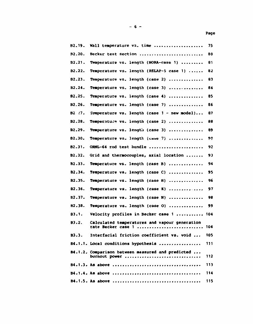
- 6 -
Page
B2.19. Wall temperature vs. time 75
B2.20. Becker test section 80
B2.21. Temperature vs. length (NORA-case 1) 81
B2.22. Temperature vs. length (RELAP-5 case 1) 82
B2.23. Temperature vs. length (case 2) 83
B2.24. Temperature vs. length (case 3) 84
B2.25. Temperature vs. length (case 4) 85
B2.26. Temperature vs. length (case 7) 86
B2 il. Temperature vs. length (case 1 - new model)... 87
B2.28. Temperature vs. length (case 2) 88
B2.29. Temperature vs. lengt'a (case 3) 89
B2.30. Temperature vs. length (caa« 7} 90
B2.31. ORML-64 rod test bundle 92
B2.32. Grid and thermocouples, axial location 93
B2.33. Temperature vs. length (case B) 94
B2.34. Temperature vs. length (case C) 95
B2.35. Temperature vs. length (case R) 96
B2.36. Temperature vs. length (case K) .... 97
B2.37. Temperature vs. length (case N) 98
B2.38. Temperature vs. length (case O) 99
B3.1. Velocity profiles in Becker case 1 104
B3.2. Calculated temperatures and vapour generation
rate Becker case 1 104
B3.3. Interfacial friction coefficient vs. void ... 105
B4.1.1. Local conditions hypothesis Ill
B4.1.2. Comparison between measured and predicted ...
burnout power 112
B4.1.3. As above 113
B4.1.4. As above 114 B4.1.5 . As above 115
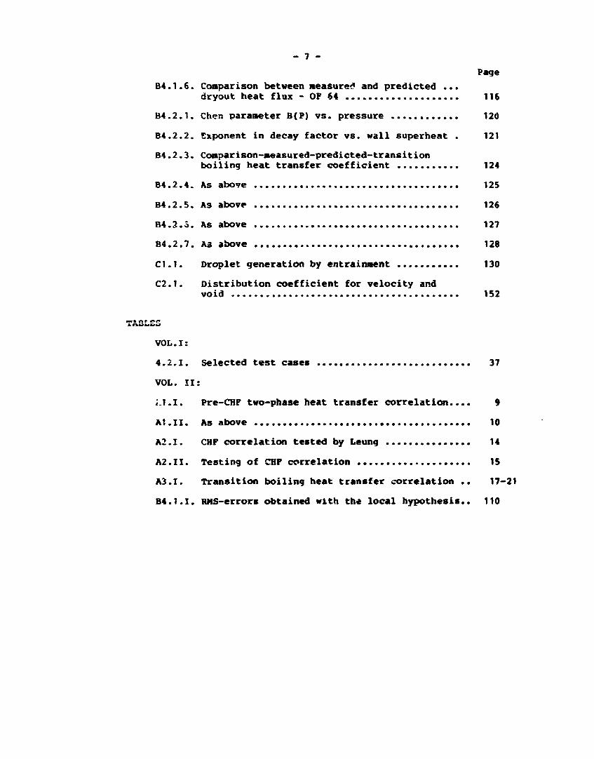
- 7 -
Page
B4.1.6. Comparison between measured and predicted ...
dryout heat flux - OP 64 116
B4.2.1. Chen parameter B(P) vs. pressure 120
B4.2.2. Exponent in decay factor vs. wall superheat . 121
B4.2.3. Comparison-measured-predicted-transition
boiling heat transfer coefficient 124
B4.2.4. As above 125
B4.2.5. As above 126
B4.2.5. As above 127
B4.2.7. As above 128
C1.1. Droplet generation by entrainment 130
C2.1. Distribution coefficient for velocity and void 152
VOL.I:
4.2,1. Selected test cases 37
VOL. II:
;.1.I. Pre-CHP two-phase heat transfer correlation.... 9
At.II. As above 10
A2.I. CHF correlation tested by Leung 14
A2.II. Testing of CHF correlation 15
A3.I. Transition boiling heat transfer correlation .. 17
B4.1.I. RMS-errors obtained with the local hypothesis.. 110

- 8 -
APPENDIX A. PRESENT KNOWLEDGE
A1. Nucleate boiling and forced convective boiling
A literature search is reported in.(7). Table A1.I taken from
(18) contains four of the best known correlations for nucleate
boiling and forced convective flow. Both experimental data and
comparisons with different correlations are reported. The corn-
comparisons are of correlations with experimental data typical
for steam generator conditions.
Correlations by Levy and Borishansky gave the best results with
an RMS-error of 22-23%.
Two new correlations for bulk boiling and subcooled boiling are
also presented in (18). They gave RMS-errors of 16 and 12%,
respectively, for their own experimental data. The correlations
are given in Table A1.II.
Stephan and Auracher (19) have presented new correlations for
nucleate boiling and forced convective boiling heat transfer.
The correlations are developed from a large set of data points
(5000) using regression analysis. The correlations are given in
Table A1.II.
It should be noted that these new correlations in Table A1.II
can be written in the form:
h N c B = P(B).q-A
with A ~ 0.65 - 0.7.
This is also the case for the correlations by Levy and Bo
rishansky.

TABLE A 1 . I . - 9 -
Authors
Thorn
Levy
Chen
Bor i shansky
C o r r e l a t i o n s
, q - . 1 / 2 Tw-TS A T=22.52«f J • exp( -0 .0115^P)
V 106/
P in bar
T w - T S A T = 0 . 9 1 2 8 ' q " 1 / 3 . P ~ 4 / 9
P in bar
n b = nmac + nraic
"mac • h f F
v 0 . 4 9 . r 0 . 4 5 0.49 . / k f c p f *Pf \
hmi„=0.00122•/-*—=—„ nn n . . — _ _ _ _ ] . l f f * u f # Hfg 'Pg '
/ H l 0 . 7 5 ( - J 2 J .ATSAT-S VTSAT(Vg-Vf)/
F=f | 1 ; S = f ( R e T p ) ; R e T P = R e f . P 1 - 2 5
l x t t '
h b . h p k . ( l + 7 . 1 0 9 . ( ^ j J
G / P f P g \
Pf \ Pg /
hp**h*-(wy2) h k . 0 . 0 2 3 . * . / — ) ° ' 8 - ^ f 0 ' 4
D l | i f / 0 .7
h . * 0 . 1 3 7 9 - ( P 0 , 1 4 + 1 . 8 8 ' 1 0 4 » P 2 ) ' / 5 — ) I io4 '
P i n bar
RMS with CNEN d a t a
%
59 .6
22.4
35.0
22 .9
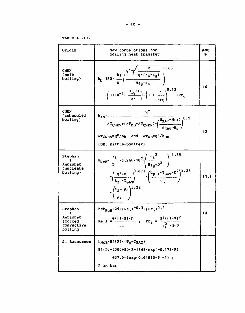
- 10 -
TABLE A1.II.
Origin New correlations for boiling heat transfer
CNEN (bulk boiling)
q"'/ *A / ' g#(P*-Pg)
,=150. _ i_ D » Hfg'Jljt
^.65
0.13
. / ,+ io-*.5i i) . i + JL\ . 1 q" ' v xttl
Frr
CNEN (subcooled boiling)
hsb=-
A T CNEN + ( A T DB- A T CNEN>' / H S A T " H t z ) j
* H S A T -H 0 /
ATCNEN^q'/hb a n d ATD B=q"/hD B
(DB: D i t t u s - B o e l t e r )
0.5
Stephan &
Auracher (nucleate boiling)
'NcB • 0 . 2 4 6
V H f g - ° / • D \0-673YCp A ' W P
•TSAJ I <\
2 N 1 . 2 6
(
PX- Pg i 5 . 2 2
PA
Stephan &
Auracher (forced convective boiling
h»hNrn.29-(Re0r0-3.(Fr0)
0-2
Re A G'(1-X)«D
Fr, G2.(1-X) 2
PI 'Ø'D
J. Rasmussen hNcBaBl(P)MTw-TSAT)
B1(P)-2000+80»P-1548'exp(-0.175«P)
+37.5»(exp(0.04815.P -1) ;
P in bar

- 11 -
The correlations by Stephan and Auracher seem to perform quite
well. They should, however, also be tested against the data
base in (18). If this test comes out well, the correlations may
be recommended for steam generator calculations.
Chen's correlation is considered as one of the best candidates
for nuclear reactor core calculations. It should be remembered,
however, that Chen's correlation is based mainly on low-pressure
data with only a few data at higher pressures (P < 70 bar). A
correlation that interpolates between Chen and Thorn is suggested
in (7) for pressures from 70 to 140 bar. This correlation is a
simplification of Chen and is much simpler to use in a computer
programme.
A2. Critical heat flux
A literature search is reported in (7). There are two classes
of CHF-situations; DNB (Departure from Nucleate Boiling) in
liquid continuous flow and DO (Dry Out) or DFCB (Departure from
Forced Convective Boiling) in vapour continuous flow.
Most of the CHF-corelations are based on the concept of equilib
rium flow with one vapour and one liquid component. The deter
mination of CHF follows, using an appropriate correlation. One
of four methods are used:
1. Heat flux versus local quality (qc/X).
("Local conditions" hypothesis).
It is assumed that there is an unique relationship be
tween CHF and l o c a l vapour quality. The method has
a tendency to fail when applied to data with strong non-
uniformity ir» axial heat flux.
2. The "Overall power" hypothesis.
This method suggests that the total power that can be
fed into a non-uniformly heated channel will be the same

- 12 -
as for a uniformly heated channel with the same geometry
and inlet conditions. No prediction of the location of CHF
is carried out. This method is found (20) to be slightly
more accurate than the above-mentioned method for axially
symmetrical non-uniform heat flux.
3. Critical quality versus boiling length (Xc/Lb).
("Equivalent length" hypothesis).
The method suggests that the CHF is not a local phenomenon
but an integral one i.e. it is dependent on the history of
what has occurred upstream. The equivalent length is de
fined as:
L. = — • J q"(z) dz
The method tends to perform better for non-uniform heat
flux situations.
4. The F-factor method by Tong.
Similar to the equivalent length method, this is an inte
gral method. The F-factor is defined as:
(q5)u F =
(qS>Nu
where (q£)u is the value of the critical heat flux at
any given local enthalpy for the uniform heat flux case
and (q£)NU is tne value of the critical heat flux at
the same local enthalpy for the particular non-uniform
heat flux case.
Another class of correlations or models are the so-called
phenomenological models, which actually attempt to model the
physical effects. Hewitt states in (21) that analytical models
on CHF produce results which are comparable in accuracy to
empirical correlations and which can be extrapolated over
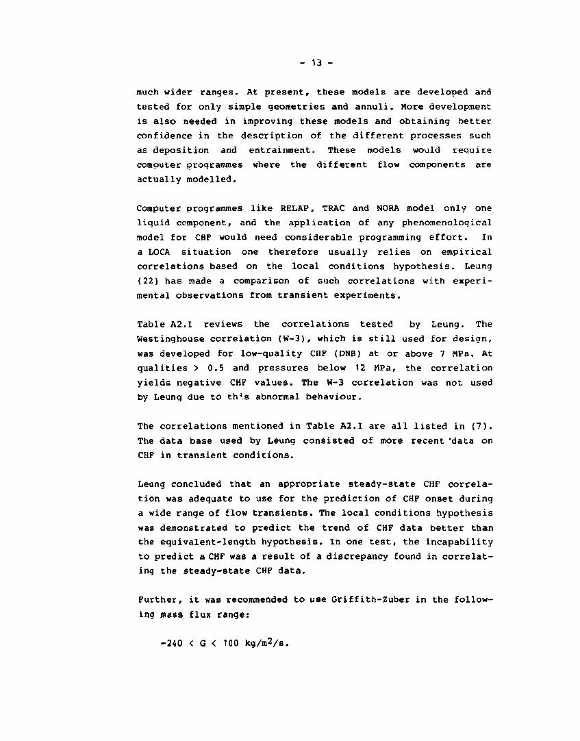
- 13 -
much wider ranges. At present, these models are developed and
tested for only simple geometries and annuli. More development
is also needed in improving these models and obtaining better
confidence in the description of the different processes such
as deposition and entrainment. These models would require
computer programmes where the different flow components are
actually modelled.
Computer programmes like RELAP, TRAC and NORA model only one
liquid component, and the application of any phenomenological
model for CHF would need considerable programming effort. In
a LOCA situation one therefore usually relies on empirical
correlations based on the local conditions hypothesis. Leung
(22) has made a comparison of such correlations with experi
mental observations from transient experiments.
Table A2.I reviews the correlations tested by Leung. The
Westinghouse correlation (W-3), which is still used for design,
was developed for low-quality CHF (DNB) at or above 7 MPa. At
qualities > 0.5 and pressures below 12 MPa, the correlation
yields negative CHF values. The W-3 correlation was not used
by Leung due to th,-s abnormal behaviour.
The correlations mentioned in Table A2.I are all listed in (7).
The data base used by Leung consisted of more recent 'data on
CHF in transient conditions.
Leung concluded that an appropriate steady-state CHF correla
tion was adequate to use for the prediction of CHF onset during
a wide range of flow transients. The local conditions hypothesis
was demonstrated to predict the trend of CHF data better than
the equivalent-length hypothesis. In one test, the incapability
to predict a CHF was a result of a discrepancy found in correlat
ing the steady-state CHF data.
Further, it was recommended to use Griffith-Zuber in the follow
ing mass flux range:
-240 < G < 100 kg/mVs.

TABLE A2.I. CHF correlations tested by Leung
Correlations
Bowring
Biasi
CISE
B & W-2
CONDIB M0D7
GE
Hsu-Beckner
Griffith
Geometry
Round tube
Round tube
Round tube
Rod bundle
Rod bundle
Rod bundle
Rod bundle
Short annulus
Pressure HPa
0.2-19
0.3-14
4.5-15
14 -16.6
3.0-17
6.9
6-15
All range
Mass flux kg/m2/s
136-18600
100- 6000
~ 100- 4000
1017- 5430
70- 4700
< 680
All
Low G
Quality
all X
- 0-1.0
~ 0-1.0
-0.03 to 0.20
-0.1 to 1.0
0-0.84
~ 0-1.0
0-1.0
Remarks
3792 points
4500 points
Freon data
Only DNB data
5163 points
Low flow data
Blowdown data
Counter current
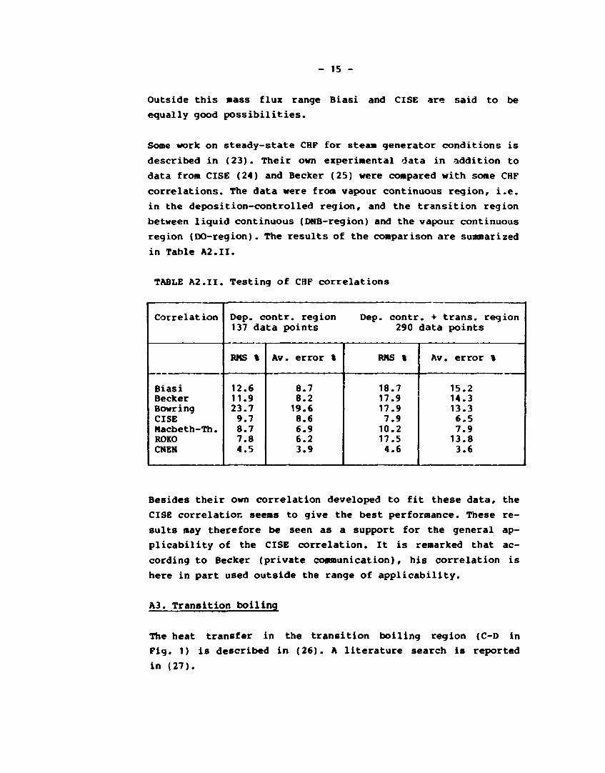
- 15 -
Outside this mass flux range Biasi and CISE are said to be
equally good possibilities.
Some work on steady-state CHF for steam generator conditions is
described in (23). Their own experimental data in addition to
data from CISE (24) and Becker (25) were compared with some CHF
correlations. The data were from vapour continuous region, i.e.
in the deposition-controlled region, and the transition region
between liquid continuous (ONB-region) and the vapour continuous
region (DO-region). The results of the comparison are summarized
in Table A2.II.
TABLE A2.II. Testing of CHF correlations
Correlation
Biasi Becker Bowring CISE Hacbeth-Th. ROKO CNEN
Dep. contr. region Dep. contr. + trans, region 137 data points 290 data points
RMS %
12.6 11.9 23.7 9.7 8.7 7.8 4.5
Av. error %
8.7 8.2 19.6 8.6 6.9 6.2 3.9
RMS %
18.7 17.9 17.9 7.9 10.2 17.5 4.6
Av. error %
15.2 14.3 13.3 6.5 7.9 13.8 3.6
Besides their own correlation developed to fit these data, the
CISE correlation seems to give the best performance. These re
sults may therefore be seen as a support for the general ap
plicability of the CISE correlation. It is remarked that ac
cording to Becker (private communication), his correlation is
here in part used outside the range of applicability.
A3. Transition boiling
The heat transfer in the transition boiling region (C-D in
Fig. 1) is described in (26). A literature search is reported
in (27).
- 16 -
Groeneveld gives in (28) an excellent review of post-CHF heat
transfer up to ~ 1974. Table A3.I shows three newer transition
boiling heat transfer correlations from his compilation (nos.
1 to 3).
A few correlations have been published since then. In Table A3.I
two correlations are shown. Number 4 is the correlation by Chen
et al. (29). The correlation is together with no. 1 an attempt
to make a phenomenological correlation. The last correlation
in the table (no. 5) is an example of a purely empirical one.
It is proposed by Bjornard and Griffith and used in TRAC.
Iloeje et al. (30) proposed a 3-step model as indicated in the
table and illustrated in Fig. A3.1. Iloeje has only one step
covering the contact period, B, C and D in Fig. A3.1. Chen uses
also a 3-step model with all 3 steps in the touching period:
waiting period, bubble nucleation- and growth-period and a
liquid film evaporation period. Convection to bulk vapour is
calculated using the Reynold's momentum analogy modified by
Colburn.
The fraction of wall hit and wetted by droplets is determined
empirically from experimental data taken from 8 different ref
erences (4167 points) ranging in pressures from 4 to 195 bar,
mass fluxes from 15 to 3000 kg/m2/sec, heat fluxes from 3 to
165 watt/cm2 and equilibrium qualities from 0.5 to 1.7.
The fraction is determined using the relation:
qT-qvc FL =
qf,c-<*vc
where qfl is the total heat flux, qvc the convective heat
flux calculated, as mentioned above, and qf,c the liquid con
tact heat flux.
The liquid contact area fraction, or the decay factor as de
signated by Tong and Young (see below), FL could be correlated
as:
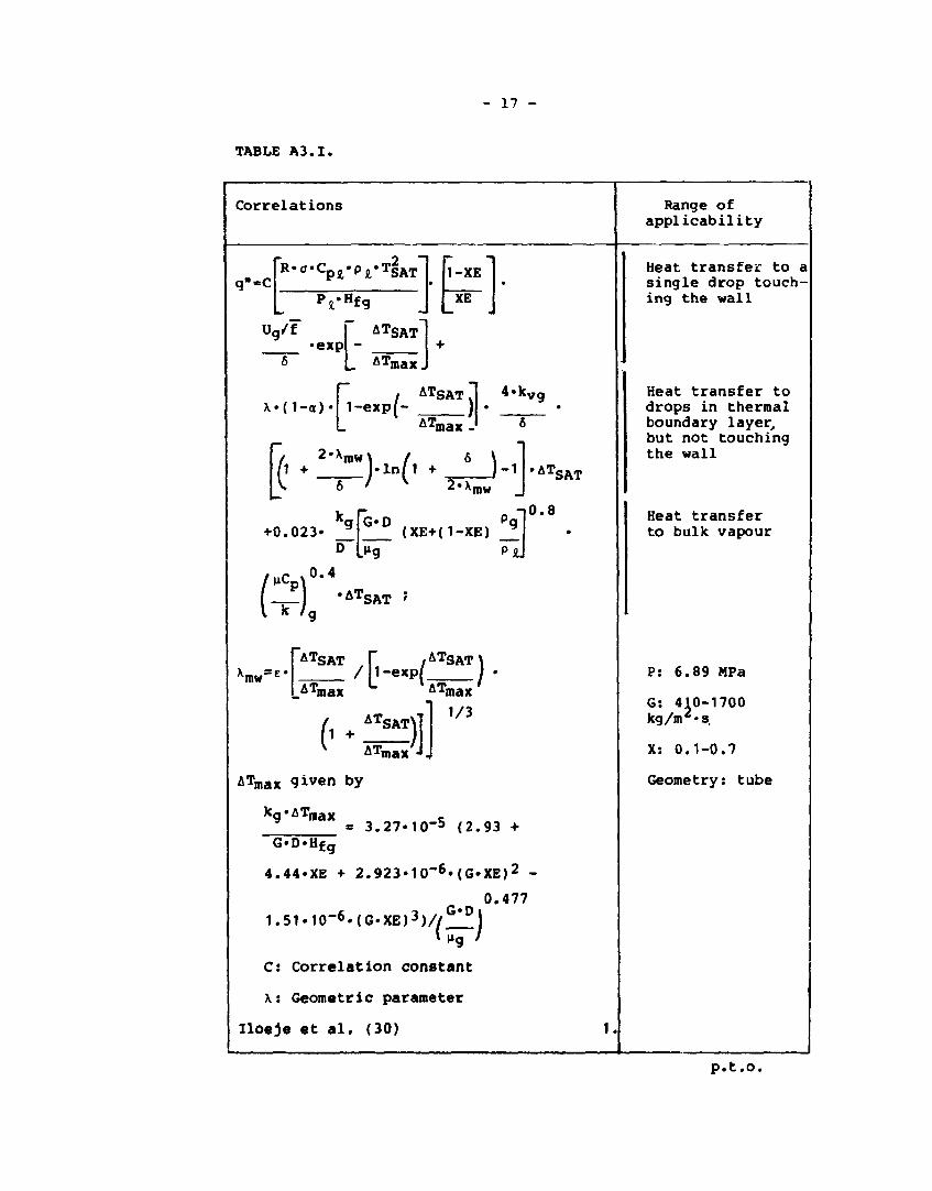
17 -
TABLE A3.1.
Correlations Range of applicability
q"=C R . a . C p z . p £ - T | A T
P.« r H f g
1-XE
XE
Ug/f
•"{" ATSAT]
AT,
X « ( 1 - a ) ' 1 -exp( -
r ATSATH 4 * k vg
AT, )
max ' I *
(i+!^Wi+J_)-il
I[G»D
'bg~
-AT SAT
+0.023« (XE+(1-XE)
(?) 0.4
-AT SAT '
xmw= E ' ATSAT
/ LATmax
f ,AT S A T t [l-exP( • w ATmay
V AT,
SAT\T
max J 4
max 1/3
ATmax given by
k g'AT m a x » 3.27.10~5 (2.93 +
G'D'Hfg
4.44.XE + 2.923»10~6«(G»XE)2 -
0.477
1.51»10~6«(G»XE)3)//G*P)
C: Correlation constant
\: Geometric parameter
Iloeje et al. (30) 1.
Heat transfer to a single drop touching the wall
Heat transfer to drops in thermal boundary layer, but not touching the wall
Heat transfer to bulk vapour
P: 6.89 MPa
G: 410-1700 kg/m2«s.
X: 0.1-0.7
Geometry: tube
p.t.o.
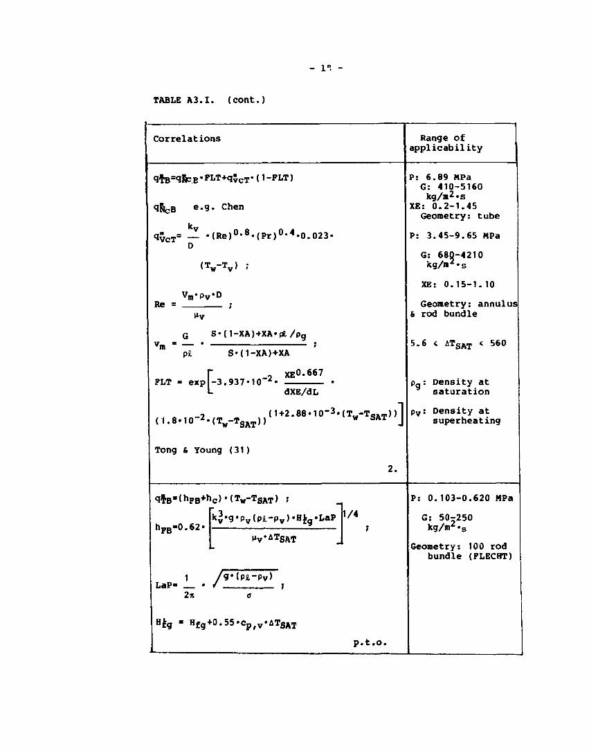
- 1«* -
TABLE A3.I. (cont.)
Correlations Range o f a p p l i c a b i l i t y
9TB= (3fc:B , p L T*<IvcT* (1-PLT)
<jRcB e - 9 - c h e n
q - c T = _Z • ( R e ) 0 ' 8 « ( P r ) 0 * 4 « 0 . 0 2 3 -0
( T w - T v ) ;
vm*Pv*D Re = ^v
'm
G S ' (1-XA)+XA'p( l /pg . ;
pi S'(1-XA)+XA
X E 0 - 6 6 7
h PLT = exp - 3 . 9 3 7 * 1 0 »-2. dXB/dL
_o ( 1 + 2 . 8 8 » 1 0 _ 3 » ( T M - T e » T ) ) I ( 1 . 8 . 1 0 2 ' ( T W - T S A T ) ) 1 w SAT j
Tong & Young (31)
2.
P: 6 . 8 9 MPa G: 4 1 0 - 5 1 6 0
k g / m 2 . s XE: 0 . 2 - 1 . 4 5
G e o m e t r y : t u b e
P : 3 . 4 5 - 9 . 6 5 MPa
G: 68Q-4210 kg/in2« s
XE: 0 .15 -1 .10
Geometry: annulus 6 rod bundle
5.6 < AT S A T < 560
pg: Density at saturation
pv: Density at superheating
qTB"( h FB + h c )* ( T w- T SAT> '
h p B « 0 . 6 2 « fcv'9*Pv<P*"Pv>,Hfg,Lap 1/4
**v*ATSAT
LaP» 1 / g » ( p £ - p v )
2*
Hfg « H f g + 0 . 5 5 . C p , v . A T S A T
p . t . o .
P : 0 . 1 0 3 - 0 . 6 2 0 MPa
G: 50-250 kg/ in2 . s
G e o m e t r y : 100 r o d b u n d l e (PLECHT)
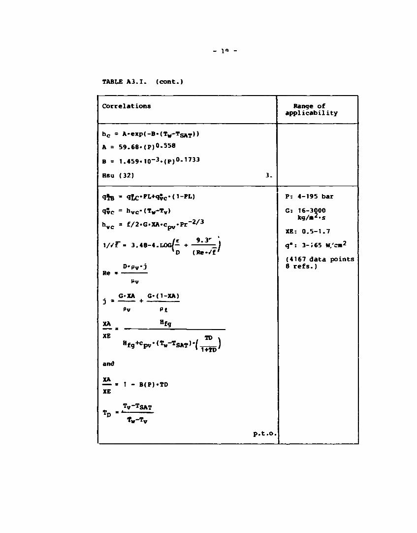
- 1« -
TABLE A 3 . I . ( c o n t . )
Corre lat ions
h c = k-expl-B'iTv-Tsxf))
A = 5 9 . 6 8 . { P ) 0 . 5 5 8
B = 1 . 4 5 9 « 1 0 ~ 3 » ( P ) 0 - 1 7 3 3
Hsu (32) 3 .
<!TB ' q t c ^ W ^ c ' C ' - « " )
<lvc = hvc*<Tw~Tv)
h v c = f / 2 . G . X A . C p w . P r " 2 / 3
1 / / F = 3 . 4 8 - 4 . LOG/- + '-—-) l D ( R e - / f '
D»pv«j Re «
t»v
G«XA G'(I-XA) j * +
Pv Pt
XA H£g
XE , TO \
ig pv »«i j 1 + T D '
and
XA « 1 - B(P)«TD
XE
Ty-TSAT T D , i
Tw-Tv
p . t . o .
Range of a p p l i c a b i l i t y
P: 4-195 bar
G: 16-3000 kg /« 2 «s
XE: 0 . 5 - 1 . 7
g": 3-J65 W/cm2
(4167 data po in t s 8 r e f s . )

- 20 -
TABLE A3.I . ( c o n t . )
Correlat ions
B(P) = 0.26
<JLC qj+qfi+qc
t 1 + t 2 + t 3
Waiting period
R.o-p£-c £ » T | A T
q a =
0.213-P-H fg R , f f , TSAT /T"1-'
t i - •[ 0.24.P»Hfq«/a£ V RT
RY+I
1 - T e r n « ' T»TTSAT
k w*Pw* c i 0.5
( " W ^W - P W 1
t - )
Mucleation period
qB - o
R+ - 2 / 3 4 ( ^ + 1 ) 2 / 3 . ( ^ ) 2 / 3 . ! ]
HI R+ * TMT 2
,2
r2
•R(t) ; R(t) input
*+ ( M 1 ) * t • - # t 2 (M2)
12»afl
Ml « 2 /3 - / J- ' H fq L W ' TSAT J
SAT'
Range of a p p l i c a b i l i t y
p . t . o .
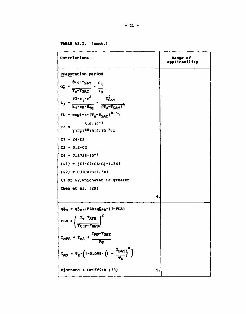
- 21 -
TABLE A 3 . I . ( c o n t . )
Correlations 1
Evaporation period
•***TSAT P,
Tw~*SAT Pq
32-p -a2 T| A T t3 *
l ,
PL « eKpC-X^T^T^y} 0- 5)
5.0-10-3
C2 » (1-«)*°+9.0.1<r3.«
CI « 24«C2
C3 * 0.2«C2
C4 - 7.3733-10'4
(XI) - (C1-C2-C4-GJ-1.341
(X2) * C3>C4*G>1.341
XI or X2, whichever is greater
Chen et al. (29)
4.
<1TB * qCHF'FLB'wrtFB*(1-pLB>
FLB - f TW"T"PB J' I TCHP-THPB'
TMS- TSAT TMPB * TMS *
TMS " T K . (1-0.095- (l - ***) )
Bjornard t Griffith (33) 5.
Range of applicability
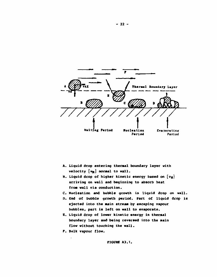
- 22 -
Period Period
A. Liquid drop entering theraal boundary layer with
velocity [VR] normal to wall.
B. Liquid drop of higher kinetic energy based on [VR]
arriving on wall and beginning to absorb heat
fro« wall via conduction.
C. Nucleation and bubble growth in liquid drop on wall.
D. End of bubble growth period. Part of liquid drop is
ejected into the aain streaa by escaping vapour
bubbles, part is left on wall to evaporate.
E. Liquid drop of lower kinetic energy in thermal
boundary layer and being reversed into the »ain
flow without touching the wall.
P. Bulk vapour flow.
FIGURE A3.1.
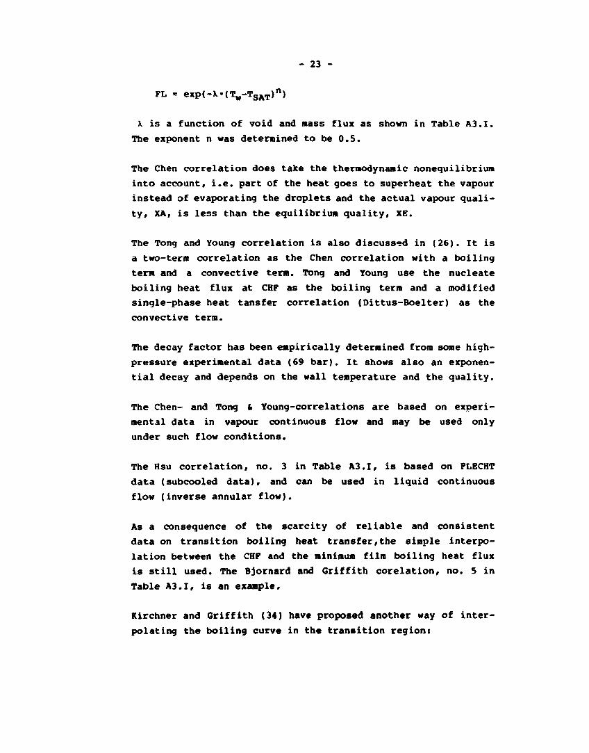
- 23 -
FL = exp(-X»(Tw-TSAT)n)
X is a function of void and mass flux as shown in Table A3.I.
The exponent n was determined to be 0.5.
The Chen correlation does take the thermodynamic nonequilibrium
into account, i.e. part of the heat goes to superheat the vapour
instead of evaporating the droplets and the actual vapour quali
ty, XA, is less than the equilibrium quality, XE.
The Tong and Young correlation is also discussed in (26). It is
a two-term correlation as the Chen correlation with a boiling
term and a convective term. Tong and Young use the nucleate
boiling heat flux at CHP as the boiling term and a modified
single-phase heat tansfer correlation (Dittus-Boelter) as the
convective term.
The decay factor has been empirically determined from some high-
pressure experimental data (69 bar). It shows also an exponen
tial decay and depends on the wall temperature and the quality.
The Chen- and Tong fc Young-correlations are based on experi
mental data in vapour continuous flow and may be used only
under such flow conditions.
The Hsu correlation, no. 3 in Table A3.1, is based on PLECHT
data (subcooled data), and can be used in liquid continuous
flow (inverse annular flow).
As a consequence of the scarcity of reliable and consistent
data on transition boiling heat transfer,the simple interpo
lation between the CHP and the minimum film boiling heat flux
is still used. The Bjornard and Griffith corelation, no. 5 in
Table A3.I, is an example,
Kirchner and Griffith (34) have proposed another way of inter
polating the boiling curve in the transition region:
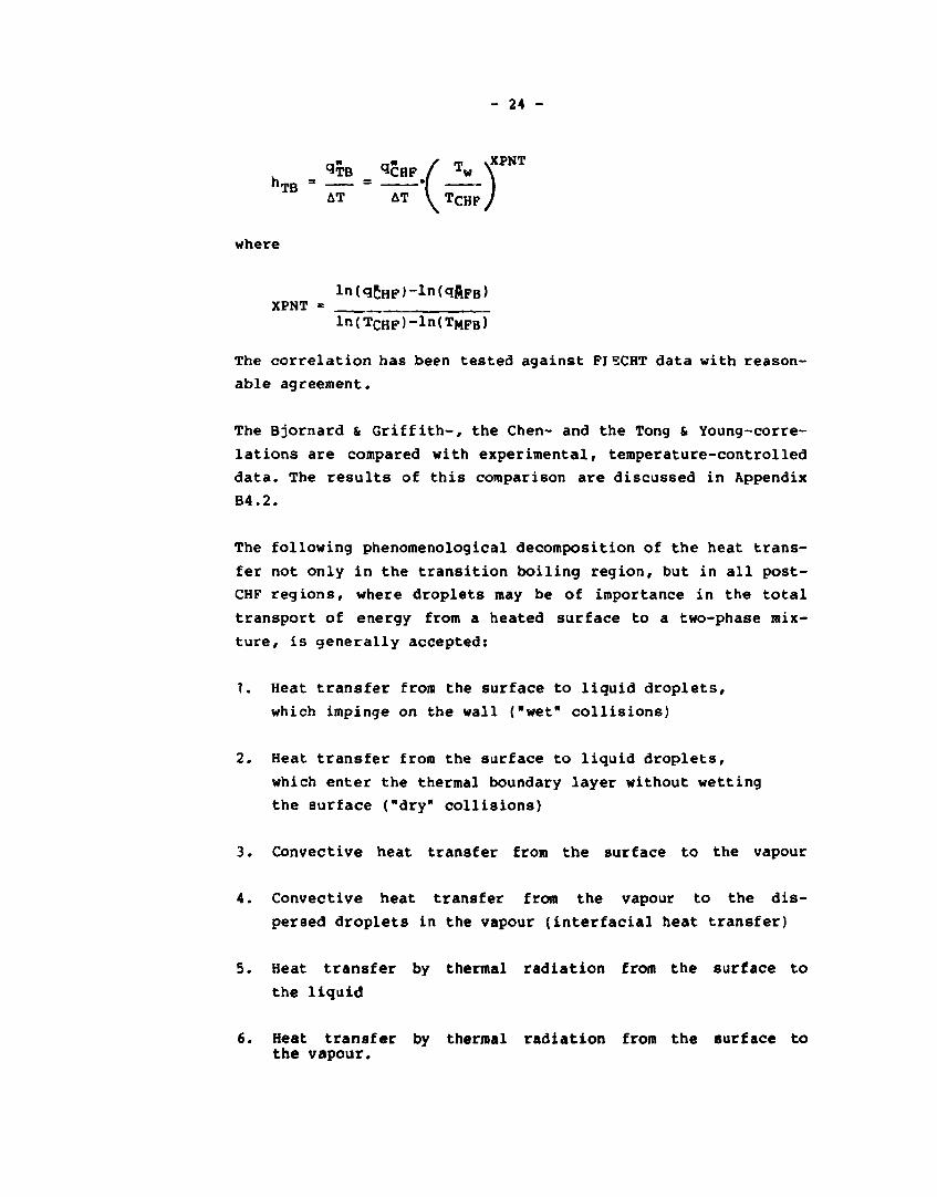
- 24 -
a" o" / T \XPNT hTB = = •( \
AT AT V ^ T C H F /
where
XPNT = ln(TCHF)-ln(TMFB)
The correlation has been tested against FIECHT data with reason
able agreement.
The Bjornard & Griffith-, the Chen- and the Tong & Young-corre
lations are compared with experimental, temperature-controlled
data. The results of this comparison are discussed in Appendix
B4.2.
The following phenomenological decomposition of the heat trans
fer not only in the transition boiling region, but in all post-
CHF regions, where droplets may be of importance in the total
transport of energy from a heated surface to a two-phase mix
ture, is generally accepted:
1. Heat transfer from the surface to liquid droplets,
which impinge on the wall ("wet" collisions)
2. Heat transfer from the surface to liquid droplets,
which enter the thermal boundary layer without wetting
the surface ("dry" collisions)
3. Convective heat transfer from the surface to the vapour
4. Convective heat transfer from the vapour to the dis
persed droplets in the vapour (interfacial heat transfer)
5. Heat transfer by thermal radiation from the surface to
the liquid
6. Heat transfer by thermal radiation from the surface to the vapour.

- 25 -
A4. Rewetting
Introduction and recommendation
In the middle of 1970 the experimental and modelling work around
the rewetting mechanism by bottom reflooding and by top spray
cooling was comprehensive, but very dispersed without any well-
defined goal. The studies produced several mathematical models
and many empirical proposals for the fitting factors in the
models. In bottom reflooding and falling film cooling of the
overheated fuel rod the length of the transition boiling re
gion is short compared with other flow regions. This transition
boiling region is in fact normally considered as a rewetting
front. Due to the sharp temperature gradient over the front the
heat from the hot, unwetted part is moved to the cold, wetted
part by an axial conduction in the fuel rod cladding.
Because most of the computer programmes don't divide the heat
structure into mesh intervals on the order of few millimeters,
the usual heat structure models are unable to calculate pro
perly the axial conduction effect, although the two dimensional
heat conduction was solved for the rod structure. That is the
reason why there are good arguments for a special handling of
the rewetting mechanism in emergency core cooling programmes.
RELAP-4/M0D-6 includes a model describing the rewetting mech
anism with the moving-mesh techniques. The axial conduction is
not modelled in the programme and the axial conduction effect
was replaced by an increment in the transition boiling coeffi
cient. The result, e.g. from the CSNI standard problem 7 for
reflooding indicated that no universally good user dials may
be proposed for RELAP-4/Mod-6 users, when the transition boil
ing approach has been used,
RELAP5/Mod2 includes a rewetting model that uses the two-
dimensional heat conduction equation for the core heat slabs.
In the rewetting front the programme doubles or halves the
structure nodes, depending on the temperature gradient in the
rewetting front. The recommendation for fixed-core heat slab
- 26 -
dimensions is on the order of 0.10 m. For the fine-mesh division
a minimum mesh length of 0.001 m is recommended. According to
earlier calculations as well as the numerical study with the
PHOENICS programme, numerical modelling of the two-dimensional
heat conduction equations for the rewetting is close to the
analytical solution if the mesh length in the front is less
than 0.001 m. Thus in the rewetting calculation the recommended
minimum 0.001 m may be seen as the maximum. There has been no
known experience with the RELAP5/MOD2 rewetting model to date.
It may may be expected that the use of a very fine mesh division
increases the computation time.
The German programme for emergency core cooling (PLUT), having
six field equations has been developed in the last 7 years and
results obtained for the reflooding process show a good agree
ment with experimental results. The programme applies the old
techniques where the axial conduction is modelled with a
mathematical correlation and usually with two fitting factors.
Work reported in (35) showed that the experimental data pub
lished in the 1970's and expressed as correlations with fitting
factors gave a large scatter between different proposals for
the fitting factors in the correlations. The correlations are
asymptotic solutions of the original differential equations.
The advantage with this kind of correlations is that in the
temperature solution only one halving procedure is needed for
the axial heat structure around the rewetting front and thus
no extra computing time is needed for the fine mesh.
Due to these experiences two possibilities may by seen with re
spect to the rewetting modelling. The classical method describing
the rewetting mechanism as a mathematical formula and as fitting
factors in it may be recommended as one possibility. The method
may be recommended especially when large computational times
for the fine mesh structure have to be avoided.
The other possibility is the method using the fine-mesh tech
niques, i.e. the coarse mesh interval around the rewetting
front is divided into a fine mesh ranging from 0.0002 to 0.001 m.

- 27 -
The method may be recommended if the computing time is avail
able. If meshes are used that are too coarse for the revetting
front, the revetting speed resulting from the calculation
deviates totally from the exact solution. Thus the method is
recommended only if a sufficiently fine mesh is possible to
use. In many applications the exact modelling of temperatures
close to the revetting front is not as interesting as the maxi
mum -jail temperatures.
Due to these experiences it may be recommended that the re
vetting mechanism should be described by using the classical
method:a correlation vith tvo fitting parameters. This classical
approach is considered more closely belov.
Mathematical revetting models
For reasons of simplicity the fuel rod cladding is considered
as a slab. The unstationary heat conduction may be vritten as
dT /a2T d2T\ p-c _ - k/ + \ (1
at V ay2 az2 J
In the moving mesh method this equation is solved numerically.
For the space derivatives the space-centred differencing may
be used. For the time derivative only the backward differencing
is possible, i.e. the implicit solution and thus the solution
needs a matrix inversion technique. The solution of the tvo-di-
mensional, time-dependent heat conduction equation is included
into RELAP5/MOD2 and TRAC and the equation is solved for core
fuel rods. Around the revetting front the heat structure is
halved in the axial and radial directions if the temperature
difference betveen tvo adjacent mesh cells becomes too high.
In the formulation of the mathematical correlation for the
revetting front the time-dependent heat conduction equation
(1) is transformed by assuming moving coordinates that move vith
the velocity of the revetting front. The revetting velocity
is assumed to be constant. The transformation applies the
relationship:

- 28 -
5T 5T a* 3T = • = u- (2
at az at dz
Further, via relationships:
T-TgAT 8 = , TQ * quenching temperature (3
To-TSAT
TI = z/5 , 6 = wall thickness (4
C - y/6 (5
h»6 Bi = h * heat transfer coefficient (6
kw
6- pw • c*u
Pe = (7 kw
The nondimensional form of the equation may be written:
©TIT, + 6CC + Pe'9,, = 0 (8
The boundary conditions are:
e » o at T) = — , e « ew at T, » +- (9
ec » - o at c - 0 , ec « -Bi»e at c -1 (10
Equation (8 cannot be solved analytically only the asymptotes
may be calculated. If the wall is assumed thin and the re wet
ting velocity low, the radial derivative Bg£ may be dropped.
Further, by assuming 6W » 1, 8W • 6(TW), the solution for
the equation is a widely used formula of Yamanouehi:
Pe » Bi°'5/(«w-1) (11

- 29 -
The two-dimensional approximation nay be formulated as the a-
symptotic solution for the original equation, by assuming a
large rewetting velocity (Pe large) and Pe > Bi. The asymptote
of the pure two-dimensional formulation is not very practical
because it strongly overpredicts the rewetting velocity at
low rewetting velocities. The use of the Yamanouchi model for
the rapid rewetting regime underpredicts the velocity, but this
can be accepted more easily than the overprediction (conser
vative).
Dua and Tien have made a useful proposal, however, which fits
the fast rewetting and slow rewetting region as well. The
calculations with the correlation have shown a good fit to
the exact solution. The work is based on the original work of
J.G.H. Andersen of Risø, and the following correlation is re
commended as a correlation for the rewetting front propagation:
Pe = (Bi*-(1 + 0.40-Bi*))0*5 (12
where
Bi Bi* = (13
ew.(6w-l)
Heat transfer correlations for the moving mesh methods
Since reflooding cases have not been included in the test
matrix in the SAK-5 project and because RELAP5/MOD2 was un
available before the end of 1984, no recommedations may be pre
sented based on computer runs for the heat transfer correlations
around the rewetting front. The heat transfer logic of RBLAP5/
MOD2 is listed, however:
• Nucleate boiling: Jens fc Lottes subcooled boiling or Chen
correlation.
• Critical heat flux: Zuber correlation multiplied by the
correction proposed by Griffith (1-a ) and multiplied by the
large flow correction (G/67.82) °*33 , if the mass flux
G > 67.82 kg/m2«s.
• Transition boiling: Weissman correlation.

- 30 -
Fitting parameters for the correlation
The fitting parameters in the correlation are the heat transfer
coefficient h in the Biot number Bi and the nondimensional re-
rewetting temperature 0O.
Previous work (35) showed that the proposal based on the ex
perimental work of the 1970's is not directly useful due to
large scatter. The German FLDT programme, using the rewetting
velocity correlation, and RELAP5/MOD2 have similar proposals
for the critical heat flux. The proposed critical heat flux may
therefore be used as a basis of the heat transfer correlation.
It is recommended that the heat transfer coefficient in Biot's
number be determined from the Zuber critical heat flux correla
tion multiplied by the Griffith's correction factor (1- a ).
The Weisraan correction (G/67.82) °»33 may be used as well. The
heat transfer coefficient is calculated by dividing the critical
heat flux by the temperature difference A TCHF = TW,CHF -Tg^Tr
which results from the heat transfer calculation in the nucleate
boiling region, where e.g. Chen's correlation is used. The
heat transfer coefficient h in Biot's number is then:
n = <1CHF»Zuber * n-<*)/UTSATf C n e n N B) (14
(For G>67.82 h = h • (67.82) °»33 may be used)
The minimum film boiling temperature may be defined as the re-
wetting temperature T0. One possibility is therefore to use
a correlation for this. Another possibility is mentioned, viz.
the choice in FLUT:
To = TSAT + 160 + 6 • ATSUD (15
The third term on the right side takes the subcooling effect
into consideration.
The recommended values should be considered as a first guess.
The functioning of the rewetting model should be tested together
with the whole heat transfer package.
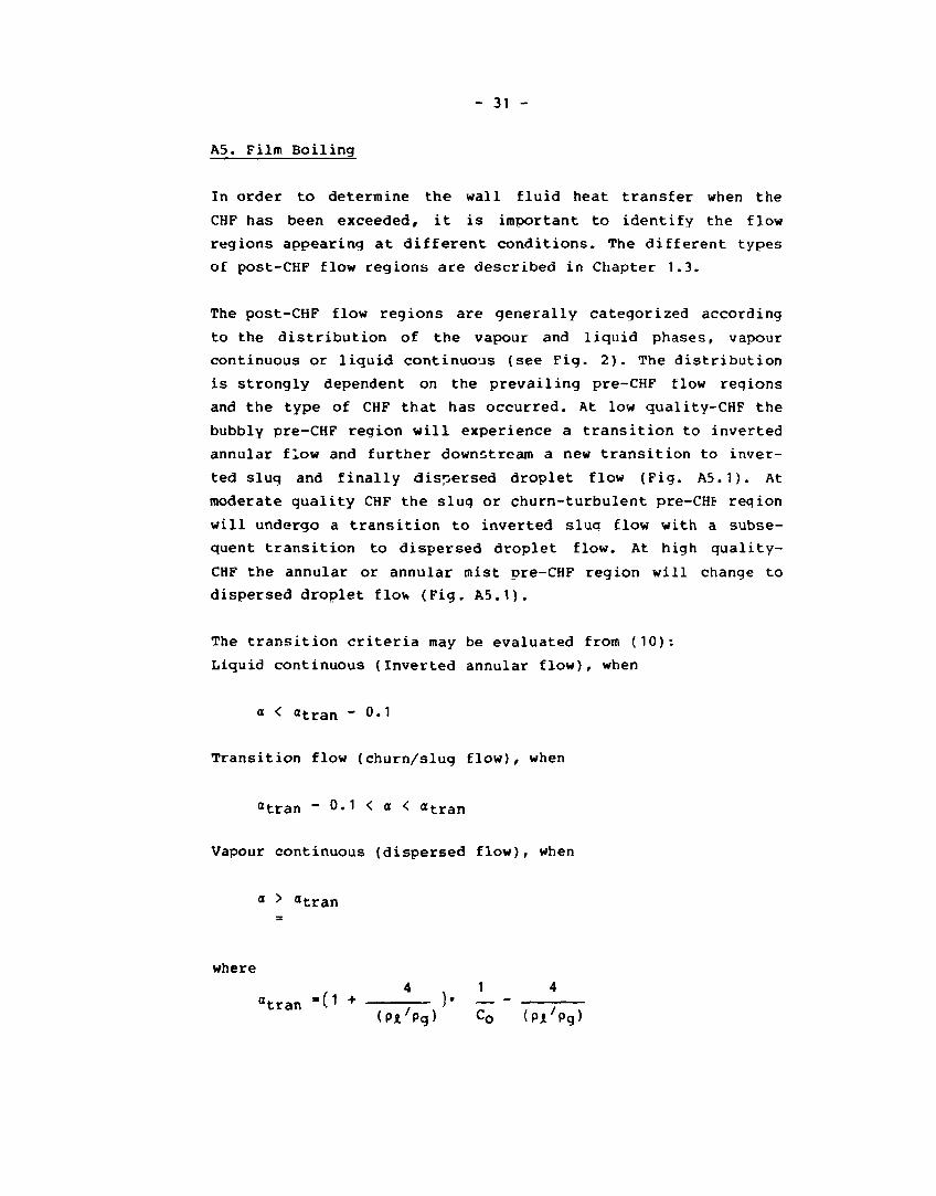
- 31 -
A5. Film Boiling
In order to determine the wall fluid heat transfer when the
CHF has been exceeded, it is important to identify the flow
regions appearing at different conditions. The different types
of post-CHF flow regions are described in Chapter 1.3.
The post-CHF flow regions are generally categorized according
to the distribution of the vapour and liquid phases, vapour
continuous or liquid continuous (see Fig. 2). The distribution
is strongly dependent on the prevailing pre-CHF flow regions
and the type of CHF that has occurred. At low quality-CHF the
bubbly pre-CHF region will experience a transition to inverted
annular flow and further downstream a new transition to inver
ted slug and finally dispersed droplet flow (Fig. A5.1). At
moderate quality CHF the slug or churn-turbulent pre-CHF region
will undergo a transition to inverted sluq flow with a subse
quent transition to dispersed droplet flow. At high quality-
CHF the annular or annular mist pre-CHF region will change to
dispersed droplet flow (Fig. A5.1).
The transition criteria may be evaluated from (10):
Liquid continuous (Inverted annular flow), when
a < <*tran - 0-1
Transition flow (churn/slug flow), when
atran - 0.1 < a < afcran
Vapour continuous (dispersed flow), when
a > atran
where 4 > 1
atran =(1 + r~ )' — " (PJl'pg) co (Pl'Pg)
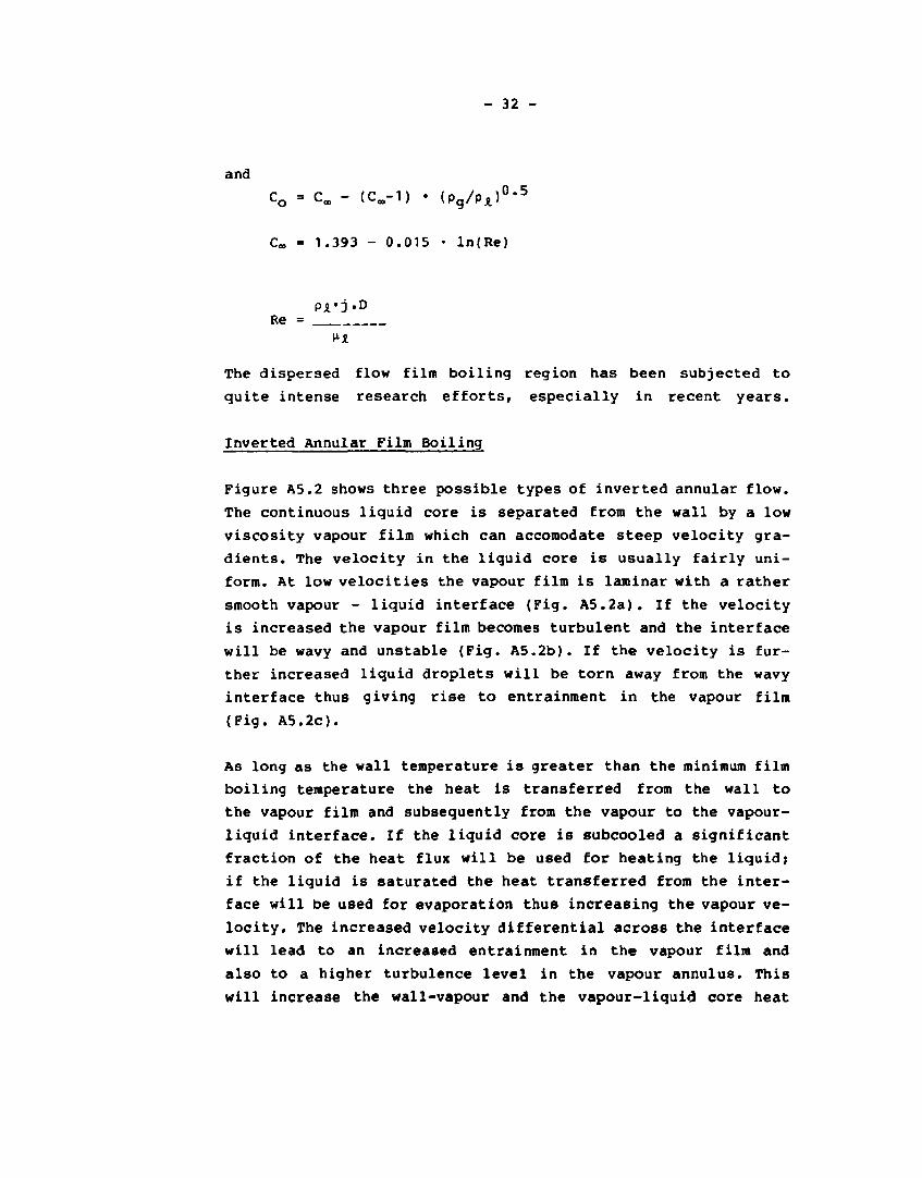
- 32 -
and
CQ = Cæ - ( C . - 1 ) • ( P g / P * ) 0 * 5
C, = 1 .393 - 0 . 0 1 5 • l n ( R e )
PJTJ'D Re =
The dispersed flow film boiling region has been subjected to
quite intense research efforts, especially in recent years.
Inverted Annular Film Boiling
Figure A5.2 shows three possible types of inverted annular flow.
The continuous liquid core is separated from the wall by a low
viscosity vapour film which can accomodate steep velocity gra
dients. The velocity in the liquid core is usually fairly uni
form. At low velocities the vapour film is laminar with a rather
smooth vapour - liquid interface (Fig. A5.2a). If the velocity
is increased the vapour film becomes turbulent and the interface
will be wavy and unstable (Fig. A5.2b). If the velocity is fur
ther increased liquid droplets will be torn away from the wavy
interface thus giving rise to entrainment in the vapour film
(Fig. A5.2c).
As long as the wall temperature is greater than the minimum film
boiling temperature the heat is transferred from the wall to
the vapour film and subsequently from the vapour to the vapour-
liquid interface. If the liquid core is subcooled a significant
fraction of the heat flux will be used for heating the liquid;
if the liquid is saturated the heat transferred from the inter
face will be used for evaporation thus increasing the vapour ve
locity. The increased velocity differential across the interface
will lead to an increased entrainment in the vapour film and
also to a higher turbulence level in the vapour annulus. This
will increase the wall-vapour and the vapour-liquid core heat

- 33 -
transfer which in turn will lower the wall teaperature. If the
wall teaperature drops below the ainiaua f ila boiling teaperature
rewetting of the wall may occur.
Different types of correlations have been developed for calculat
ing the hc.t transfer coefficient in the inverted annular flow
region (see (12)). The correlations can be divided into the fol
lowing categories:
* Correlations applicable to pool boiling conditions and
heat transfer at low aass fluxes. A well-known example of
these is the Broaley correlation. Host of the correlations
of this type have the fora
J*v*ATSAT
The latent heat Hfø is usually aodified to include the vapour
superheat while the velocity effect is included through the
function f(V,X) where x is equal either to the hydraulic dia-
aeter, the critical wavelength, or the aost unstable wavelength.
* Correlations of the aodified HcAdaas type. These correla
tions basically have the fora
Nu = a • Reb • Pre • p
where F usually is a function of quality or vapour film
teaperature.
* Phenoaenological correlations based on the different mecha-
nisas governing this type of heat transfer.
The literature search reported in (12) resulted in a recommeda-
tion to use a aodified Broaley correlation when evaluating thf
heat transfer for the inverted annular flow. This correlation
can be written as
q" « h • (Tw-TsAT)
- 34 -
K n c, r^'Pv-^X-PvJHfg-g, V4 h = 0.62 •[ _ I
Xc'Hv'ATsAT
where a 1/2 Xc = 2it*[ ]
g(Pl-pv)
Xc is the critical wavelength of Taylor instability. This
correlation seems to fit the data reasonably well within the
parameter range
Pressure 0.1 - 0.7 MPa
Wall Heat Flux 30 - 130 kW/m2
Subcooling < 78 K
Velocity < 0.3 m/s
Void < 0.4
An interesting study of the low flow film boiling heat transfer
coeffiecient of Bromley was carried out by GE, USA (36,37). In a
recent study (38) some deficiencies of the modified Bromley
models were pointed out. Specifically mentioned were the lack
of influence of the distance from the CHF location and the
exclusion of flowrate and subcooling effects. In that context
a new model was also developed, based on the Bromley type of
analysis but including the above mentioned effects. The analysis
terminated in a differential equation that was integrated numeri
cally with adequate boundary conditions. The result was compared
to some new data from a single tube reflooding experiment and
the comparison was quite satisfactory (Fig. A5.3). The result
using the modified Bromley model was much less successful, as
shown in Fig. A5.4. However ->ne major drawback with this new
model is the difficulty ot implementing it in the numerical
scheme of an already existing computer code like RELAP5 and
TRAC due to the differential form of the model.
Breakdown of Inverted Annular Flow
The breakdown of the liquid core into slugs and further down-
- 35 -
stream to droplets has also been related by some authors to a
critical Weber number based on the diameter of the liquid core
(approximately equal to the channel hydraulic diameter) and
the relative velocity between the phases at this point:
pg'(vg~v*,2*D
According to (12) a He-number of approximately 10 seems to fairly
well correlate the data obtained in reflooding experiments.
However in (38) We ~ 20 is obtained. This He-number was based
on the vapour velocity only, but as the liquid velocity was
rather small in that study the result would be only slighty
lower if the relative velocity definition was used. Thus when
a He-number of 10 to 20 is exceeded the liquid core can be
assumed to break down.
Dispersed Droplet Film Boiling Region
In the dispersed droplet flow region the liquid phase exists
as droplets of different sizes carried along in the vapour
flow. Several investigations have shown that the vapour phase
in general is superheated (12) with respect to the local satu
ration temperature while the liquid phase normally is found
to be close to saturated conditions. These nonequilibrium ef
fects have been found to be of major importance when describing
the pertinent heat transfer mechanisms and the development of
this region.
Due to the difficulty of measuring the vapour superheat when
liquid droplets are present, the exact mechanisms for the heat
transfer are poorly understood despite the intense research
efforts made during the last years. In most of the experiments
only the wall temperatures were measured and the nonequilibrium
vapour conditions had to be inferred from these temperatures
by use of a single-phase convective heat transfer correlation
and the assumption that the wall-to-droplet heat transfer was
negligible.
- 3« -
However, a leap forward was taken when a technique was developed
to measure the vapour temperature by æans of a specially de
signed aspiration thermocouple probe (39,40). In those studies
the vapour superheat was Measured at only one location down
stream of the CHF-front though, so the axial behaviour of the
nonequilibrium effect was unknown. Quite recently two experi
mental test series were conducted (41,42) in which the axial
variation of the nonequilibriua conditions downstream of the
CHF-front was also measured. Prom the results of these experi
ments it was evident that the vapour generation was quite high
near the CHP location and decreased furthet downstream. The
increased vapour generation near the CHP location was hypothe
sized to be caused by some sputtering effects when the wall
liquid film was violently driven off the wall at the CHP loc
ation (17).
This indicates that the vapour generation has to be separated
into a near field region where the vapour generation rate is
relatively high, and a far-field region with a lower vapour
generation rate. Thus, different mechanisms can be assumed to be
dominant in each region.
Prediction Methods
Basically, two main groups of models can be identified when
analyzing the approaches utilized for calculating the heat
transfer in the dispersed droplet film boiling region (12,43*:
equilibrium correlations and nonequilibrium models.
Equilibrium Correlations
This approach is based on two assumptions:
* Thermodynamic equilibrium exists between the two phases
* Heat transfer at the heated walls occur primarily by tur
bulent vapour convection.
- 37 -
This can be expressed mathematically as
q" = hc • (TW-TSAT)
The heat transfer coefficient hc is calculated from an equili
brium correlation, for instance, Groeneveld and Dougall-Rohsenow
correlations (12). Also the Condie-Bengston correlation is of
this type and is currently utilized in the RELAP5/ M0D1 computer
code (44).
When compared with experimental data these types of correlations
seem to predict reasonable trends, the quantitative disagree
ments can be substantial though (43). It is also questionable
whether these types of correlations in nonequilibrium computer
programmes like, eg. RELAP5, should be utilized (45).
Nonequilibrium Models
The nonequilibrium models recognize the importance of vapour
superheating when calculating the heat transfer. The models can
be grouped into two categories (12): a) local correlations, b)
separate phase models.
a) Local Correlations
This type of correlation calculates the local vapour superheat
and heat transfer coefficient from local thermal hydraulic para
meters. Examples are the Groeneveld-Delorme correlations and
the CSO correlation of Chen, Sundaram and Ozkaynak. Both of
these correlations are given in (12). They relate either the
actual quality or the vapour superheat and the wall heat trans
fer coefficient to such parameters as the vapour Reynolds number
and equilibrium quality. They are easy to implement into exi
sting thermohydraulic codes but due to their highly empirical
nature the prediction results usually reveal quite substantial
scatter although the average result from a large number of
calculations can be rather good.
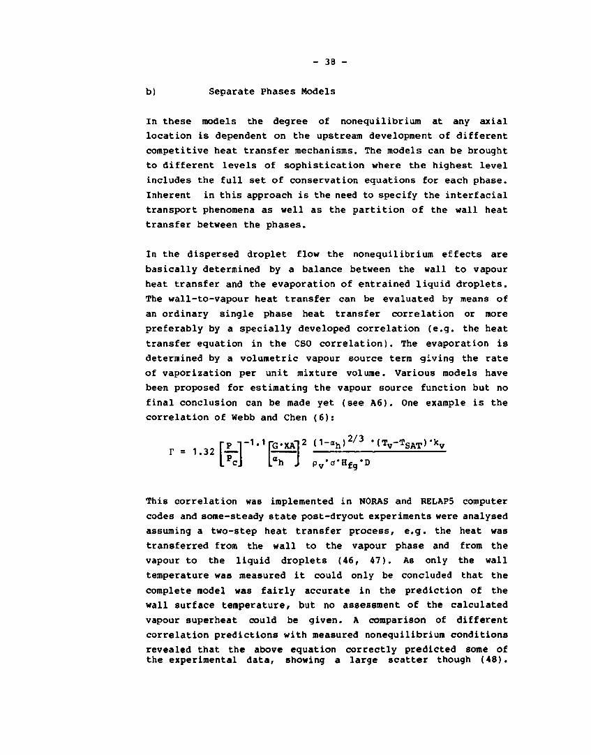
- 38 -
b) Separate Phases Models
In these models the degree of nonequilibrium at any axial
location is dependent on the upstream development of different
competitive heat transfer mechanisms. The models can be brought
to different levels of sophistication where the highest level
includes the full set of conservation equations for each phase.
Inherent in this approach is the need to specify the interfacial
transport phenomena as well as the partition of the wall heat
transfer between the phases.
In the dispersed droplet flow the nonequilibrium effects are
basically determined by a balance between the wall to vapour
heat transfer and the evaporation of entrained liquid droplets.
The wall-to-vapour heat transfer can be evaluated by means of
an ordinary single phase heat transfer correlation or more
preferably by a specially developed correlation (e.g. the heat
transfer equation in the CSO correlation). The evaporation is
determined by a volumetric vapour source term giving the rate
of vaporization per unit mixture volume. Various models have
been proposed for estimating the vapour source function but no
final conclusion can be made yet (see A6). One example is the
correlation of Webb and Chen (6):
- 1- 1r g <XA] 2 d - g h )2 / 3 MTv-TSAT)-kv
Lah J p v-a-H f g'D
This correlation was implemented in NORAS and RELAP5 computer
codes and some-steady state post-dryout experiments were analysed
assuming a two-step heat transfer process, e.g. the heat was
transferred from the wall to the vapour phase and from the
vapour to the liquid droplets (46, 47). As only the wall
temperature was measured it could only be concluded that the
complete model was fairly accurate in the prediction of the
wall surface temperature, but no assessment of the calculated
vapour superheat could be given. A comparison of different
correlation predictions with measured nonequilibrium conditions
revealed that the above equation correctly predicted some of the experimental data, showing a large scatter though (48).
r = 1.32 t
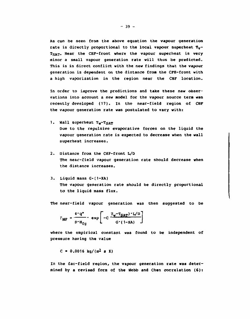
- 39 -
As can be seen from the above equation the vapour generation
rate is directly proportional to the local vapour superheat Tv-TSAT« Near the CHF-front where the vapour superheat is very
minor a small vapour generation rate will thus be predicted.
This is in direct conflict with the new findings that the vapour
generation is dependent on the distance from the CFH-front with
a high vaporization in the region near the CHP location.
In order to improve the predictions and take these new obser
vations into account a new model for the vapour source term was
recently developed (17). In the near-field region of CHF
the vapour generation rate was postulated to vary with:
1. wall superheat Tw-TgAT
Due to the repulsive evaporative forces on the liquid the
vapour generation rate is expected to decrease when the wall
superheat increases.
2. Distance from the CHP-front L/D
The near-field vapour generation rate should decrease when
the distance increases.
3. Liquid mass G-(I-XA)
The vapour generation rate should be directly proportional
to the liquid mass flux.
The near-field vapour generation was then suggested to be
4-q- f Tw-TSAT)-L/Dl rNP exp -c
D*Hfg L G*(1-XA) J
where the empirical constant was found to be independent of
pressure having the value
C » 0.0016 kg/{jn2 s K)
In the far-field region, the vapour generation rate was deter
mined by a revised form of the Webb and Chen correlation (6):
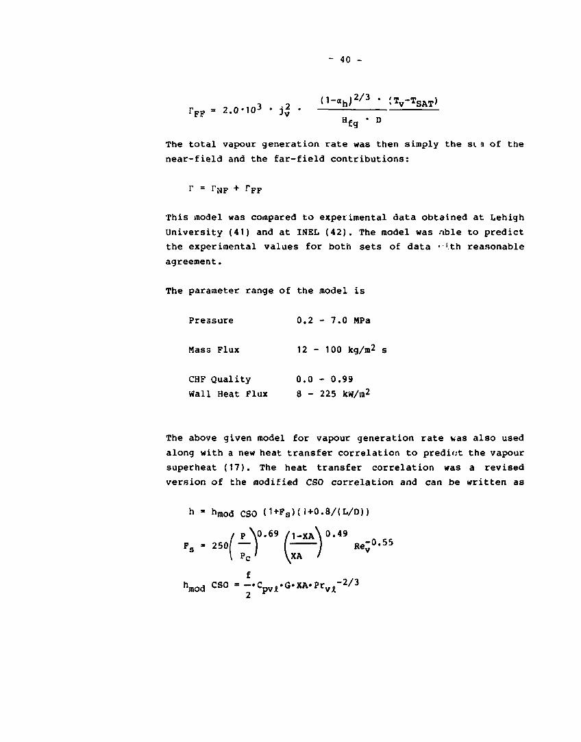
- 40 -
,«3 -2 d-g hJ2 / 3 • '>TV-TSAT)
rFP = 2.o-ioJ • J* -
Hfg ' D
The total vapour generation rate was then simply the si a of the
near-field and the far-field contributions:
r - rNF + rFF
This model was compared to experimental data obtained at Lehigh
University (41) and at INBL (42). The model was .nble to predict
the experimental values for both sets of data • >th reasonable
agreement.
The parameter range of the model is
Pressure 0.2 - 7.0 MPa
Mass Flux 12 - 100 kg/ra2 s
CHF Quality 0.0 - 0.99
Wall Heat Flux 8 - 225 JcW/m2
The above given model for vapour generation rate was also used
along with a new heat transfer correlation to predict the vapour
superheat (17). The heat transfer correlation was a revised
version of the modified CSO correlation and can be written as
h " hmod CSO (1+Fs)(l+0.8/(L/D))
A 0 , 6 9 /I-XA\O-'
Fg = 2 5 0 ( - r ~ / - ^ L ) ' 4 9 Re-0.55
hmod c s o = 2'CPv**G'XA'Prvjf2/3
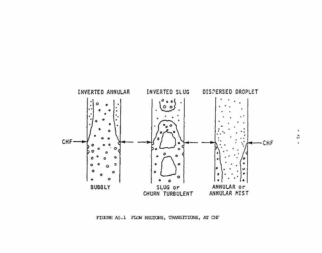
INVERTED ANNULAR INVERTED SLUG DISPERSED DROPLET
<» o SLUG or
CHURN TURBULENT
ANNULAR or ANNULAR MIST
CHF I
FIGURE A5.1 FDOW REGIONS, TRANSITIONS, AT CHF
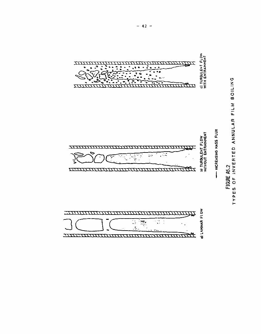
- 42 -
3*
UJJC
o z
o CD
\ , V V \ V V \ V M l V V k ^ \ \ \ H l V V \ \ \ V V \ H H V \ . V V V V \ M A , V •"
II W H M V u \ v \ u \ \ u \ \ \ \ u \ \ \ v \ v u \ \ \ ^ u v v w n \ v 2 g
x 3
< X O z in < ui tr u z
cc <
Z
UJ I -CC UJ
°i > $± gu. 3 o C (0
UJ
o. >•

- 4 3 -
ALL OATA FOR WHICH CALCULATED WEBtR NUMBER WAS LESS THAN ?0
WO 200 300 COO
MEASURED HEAT TRANSFER COEFFICIENT W m-1 K" '
FIGURE A5.3 COMPARISON OF MEASURED ANO CALCULATED HEAT TRANSFER COEFFICIENTS -PRESENT WORK (FROM REF. 3 8 )
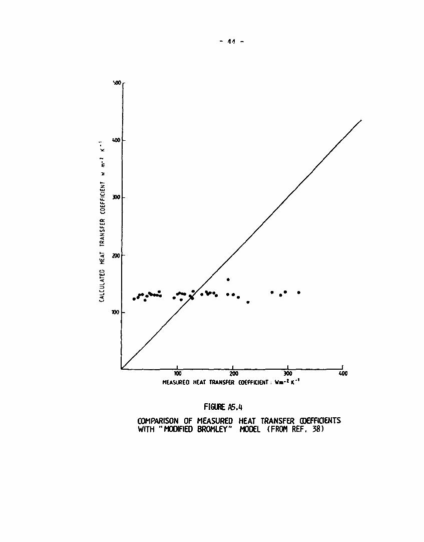
- 44 -
SOO
•
•
g
z
£ 300 u-o
CC
< 200 UJ
i :
o
• * • / • _ • •
WO
I I L_ »0 200 300
MEASUREO HEAT TRANSFER COEFFICIENT : W«r* K . i «X>
FIGURE A5.1
COMPARISON OF MEASUREO HEAT TRANSFER COEFFICIENTS WITH "MODIFIED BROMLEY" M00EL (FROM REF. 38)

- 45 -
T -0.1
v - — i
— 9 - 3 5
0 + Rev /£
The predicted vapour superheat from this film boiling model was
compared with nonequilibrium experimental data. There was still
some scatter but the model was an improvement compared to earlier
models.
A6. Interfacial Heat Transfer
When a two-fluid model is used, interfacial mass-transfer rate
r is calculated from
QiA + Qig
r = Hfg
where Qn is the heat transferred from the interface to the
liquid phase, Qig is the heat transferred from the interface to
the vapour phase and Hfg is latent heat of evaporation. The
interfacial heat transfer rates are calculated from
Qik * hik'(Tk " TSAT>
where T is the temperature, h ^ is the volumetric heat transfer
coefficient, and the subscript k is either I or v. Some correlations are expressed in terms of enthalphy or quality. From a
computational point of view the use of enthalphy instead of
temperature is more convenient, because usually enthalphy (or
enthalpies) is one of the dependent variables to be evaluated.
All the correlations can be transformed to a suitable form,
for example hik
Qik " (Hk " «kSAT> cpk
where Cpfc is specific heat.
"Z = 3.48 - 4*log10
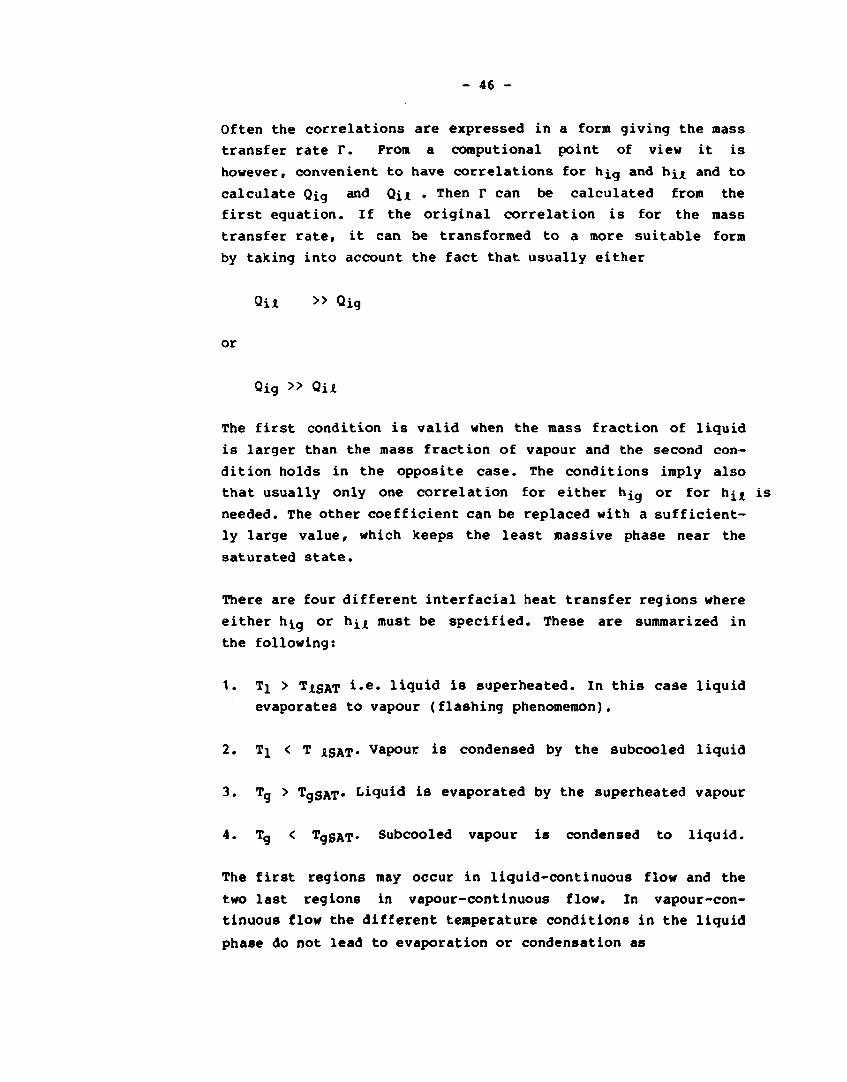
- 46 -
Often the correlations are expressed in a form giving the mass
transfer rate r. From a computional point of view it is
however, convenient to have correlations for h^g and hn and to
calculate Qig and Qn . Then r can be calculated from the
first equation. If the original correlation is for the mass
transfer rate, it can be transformed to a more suitable form
by taking into account the fact that usually either
QiA » Qig
or
Qig » Qi*
The first condition is valid when the mass fraction of liquid
is larger than the mass fraction of vapour and the second con
dition holds in the opposite case. The conditions imply also
that usually only one correlation for either hjg or for h^j is
needed. The other coefficient can be replaced with a sufficient
ly large value, which keeps the least massive phase near the
saturated state.
There are four different interfacial heat transfer regions where
either h^g or h ^ must be specified. These are summarized in
the following:
1. Ti > TJISAT i*e« liquid is superheated. In this case liquid
evaporates to vapour (flashing phenomemon).
2. Ti < T jtsAT« Vapour is condensed by the subcooled liquid
3. Tg > TggAT* Liquid is evaporated by the superheated vapour
4. Tg < TgSAT- Subcooled vapour is condensed to liquid.
The first regions may occur in liquid-continuous flow and the
two last regions in vapour-continuous flow. In vapour-con
tinuous flow the different temperature conditions in the liquid
phase do not lead to evaporation or condensation as
- 47 -
described in i teas 1 and 2, because the flashing rate is con
trolled by Qiq. The saae concerns the vapour phase in the low
quality region. Four different correlations for interfacial
heat transfer are therefore needed, two for h^ i and two for hjo. Furthermore, the correlations used for evaporation or condensa
tion must be continuous at the point T^ = T^gAT' because dis
continuity may trigger an instability, where mass transfer rate
and pressure are oscillating.
In addition to the flow boilinq, a wall boiling (or conden
sation) model must be specified. In that case the total mass
transfer rate I*tot *s
ftot 3 r + rq
where r is calculated from the first equation and the mass
transfer rate at the wall Pw is calculated using a separate
model. This kind of model is needed for suncooled boilinq, be
cause in that case no evaporation is predicted using the two
first equations. Another case is condensatipon of vapour at the
cold wall. In these cases both rw and I* must be tailored so
that the total mass transfer rate is correct.
Although the interfacial heat transfer is of great inportance
in all two-phase flow calculations, very few empirical cor
relations exist at present. Very often the lack of a correla
tion must be compensated for by using a suitable large value for
the interfacial heat transfer coefficient. This approach has
also been used in the large system programmes like RELAP5 (see
for example Appendix B3). Furthermore, in many cases the corre
lation developed are "semi-empirical", which means that a
correlation is based on an analytical approach and it is tuned
using some experimental data, very often this tuning is based
on a limited number of tests and consequently the correlation
is not a reliable one for general purposes.
In SAK-5 work interfacial heat transfer correlations have been
tested for flashing and for post-dryout heat transfer (50,
46). In the case of flashing the correlations were tested by
- 48 -
calculating blowdown-experiments where the pressure undershoot
below the saturated value is significant (51, 52), and by
calculating critical flow experiments (52, 53). Five different
correlations were tested and only the correlation of Bauer et
al. was satisfactory. This correlation is a simple relaxation
type model
r XE-XA
p i
where XA is the actual quality, XE is equilibrium quality, p is
density and i is time constant. In the case of flashing the
condition Qi* >> Qig holds and the following heat transfer
coefficient is obtained
(1-g)'pj'Cpi hii =
T
the time constant x has been correlated using Moby Dick test as
660 x = _ (a+ a0)(u+u0)
z/P~
where a is void fraction, u is velocity in m/s and P is pressure
in N/m . In the original model <xQ = uQ = 0, but in that case
the above equation for -c cannot be used for initial flashing.
The correlation is valid in the range of 0.01 < a < 0.96 and
5 m/s < u < 54 m/s. In the present work the correlation has
been extrapolated to cover also the early flashing process. For
that purpose the constants were determined to be
a0 • 0.003
u0 * 4 m/s
- 49 -
These values are so small that they do not significantly change
the correlation within its validity range, but they predict
reasonable values for hn when a = 0 or u = 0. An alternative
for this approach is presented in (54), where the time constant
is the minimum of T calculated from the above equation and the
following
2.7 • 10~ 5H| x = 1
This approach has not been tested in the present work. When the
first approach is used to predict the pressure recovery during
the blowdown, the result seems to depend on the flow area. When
medium-size pipes (D ~ 0.5 m) are simulated the calculated re
sult is close to the experimental one (see Pig. A6.1). When the
diameter is smaller, as in Edwards' pipe test, the predicted
pressure recovery is too slow.In the case of a large vessel the
predicted pressure recovery is too fast (50). This kind of de
viation from the experimental data is not so harmful because
the error is significant during only a very short period. Fur
thermore, it is difficult to obtain better results, because the
initial flashing is a complicated phenomenon depending on
soluble gases, surface roughness etc. It is obvious that in
many cases the flashing correlation must be tuned in order to
take into account these effects properly.
Better results were obtained from critical flow calculations.
When the pipe length was 0.14 m and the diameter 0.014 m, the
calculated results were close to the experimental ones on
pressure range from 0.3 MP a to 9 MPa (Pig. A6 2). When the
pressure was fixed, the correlation was able to predict the
increase in mass flux when the pipe length was decreased (Pig.
A6.3).
Because at present it seems that there are no better correlations
for flashing, Bauer's correlation is recommended. In the test
cases calculated it gave moderately good results.

- *>0 -
• o «
• X
X'
^
x;
-X"
z o
Uio «X" •o
X'
• •
c \
\ v
S • • '
" ^ ^ ^ ^ ^
1 1 1 1 1 1 1 1 1 I 1 1 M 0 -M «.M l - M I . M I . M < . ! •
HUE SEC
i
i
i
i r i i i ! . « • *.T» J M
Pig.A6.1 OECD Standard Problem Ko. 6. Measured ( ) and
calculated { ) pressures at the exit node. The
correlation of Bauer et al. is used for interfacial
heat transfer.
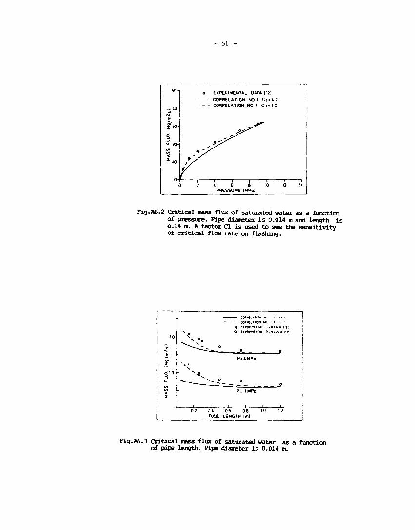
- 51 -
so-
- U 3 -
E
f 3 0
X
"̂ 20-i / i i/> <
7
0
o EXPERIMENTAL OAfA (12!
CORRELATION NO i C i ; 1 0
*1s
I I 1 1 i 1 1 2 i 6 8 10 12 U
PRESSURE (M?o)
Fig.A6.2 Critical mass flux of saturated water as a function of pressure. Pipe diameter is 0.014 m and length is o,14 m. A factor CI is used to see the sensitivity of critical flow rate on flashing.
20
6
Z
x 10
i/i »/i < X
— conmiAticm NO • r, •. •• r. x (ixaiPtiiTftL -J . o « » » HJI O fnt*MnT»l ti .oo?S »!'Jl
- ° - - - p P=tMPo
P= IMPa
0? 0 1 0 6 0 8 TUBE LENGTH |m)
10 12
Fig.A6.3 Critical mass flux of saturated water as a function of pipe length. Pipe diameter is 0.014 m.

- 52 -
APPENDIX B COMPARISON WITH DATA
B1 Heat Transfer Package.
B1.1 RELAP-5
The heat transfer package of RELAP5/M0D1 was originally developed
for the RELAP4-programme. In RELAP4 thermal equilibrium between
the phases was assumed. RELAP5/M0D1 is a nonequilibrium pro
gramme, which utilizes only one energy equation for the thermal
energy mixture . It is therefore possible to use the same heat
transfer package as in RELAP4. However, certain modifications
have to be made, because several heat transfer correlations are
based on variables used in equilibrium calculations. When the
calculation is based on a nonequilibrium assumption these va
riables must be calculated using the dependent variables of the
nonequilibrium programme. An example is the equilibrium flow
quality used in several critical heat flux correlations. The
equilibrium quality is not directly solved in computer program
mes, that allow thermal nonequilibrium.
The RELAP5/N0D1 heat transfer package (HTRC1) consists of a
forced convection (flow related) group of correlation adopted
from RELAP4/MOD6 and a pool boiling/natural convection (indepen
dent of flow) group of correlations. The low flow region is
defined for mass fluxes lower than 200 kg/m2g.
The heat transfer selection logic is based on wall temperature,
saturation temperature, equilibrium quality and void fraction.
The single-phase heat transfer to liquid is selected if equi
librium quality is lower than zero and wall temperature is lower
than saturation temperature. The single-phase heat transfer to
vapour is selected if wall temperature exceeds saturation tem
perature and void fraction exceeds 0.999. The condensation heat

- 53 -
transfer is selected if wall temperature is lowere than satura
tion temperature and the two-phase mixture temperature is greater
than the wall temperature. The nucleate boiling heat transfer is
selected if equilibrium quality is lower than the critical and
wall superheat is lower than the critical wall superheat as
calculated from the critical heat flux correlation. In other
cases the post CHF heat transfer correlations are used. The film
boiling correlations are changed to the transition boilinq cor
relation if the wall temperature is lower than the minimum film
boiling temperature,
During the SAK-5 project the heat transfer package of RELAP5/
MODI has been modified in order to use it independently. This
modification follows the original as closely as possible, but is
altered slightly for a two-fluid (six-equation) mode. For this
purpose the heat transfer coefficient has been shared between
liquid and vapour phases. In general, the separated heat transfer
part has worked well in the test calculations. Some remarks
should be made, however, especially concerning the original
RELAP5-programme. In RELAP5 the heat transfer is calculated
directly as heat flux. The heat transfer coefficient is inter
preted as the derivative of heat flux with respect to wall tem
perature and is used for the implicit inteqration of wall
temperatures. According to the RELAP5 manual, the heat transfer
coefficient of transition boiling should be negative. The pro
gramme, however, omits the negative values, perhaps for reasons
of stability.
Another remark concerns the definition of quality in the heat
transfer part. Although the static equilibrium quality may be
more reasonable from a calculational point of view, most of the
correlations have been developed using flow quality. In vertical
channels, the vapour velocity close to the crisis point may be
larger than the liquid velocity, and consequently the flow quality
is larger than the static quality. Therefore, the original corre
lation that uses flow quality, predicts smaller critical heat
flux than the same correlation in the RELAP5 package.
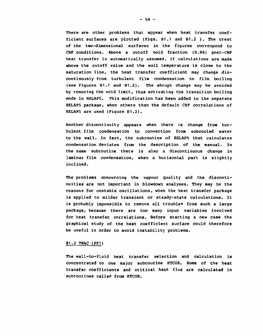
- 54 -
There are other problems that appear when heat transfer coef
ficient surfaces are plotted (Figs. B1.1 and B1.2 ). The crest
of the two-dimensional surfaces in the figures correspond to
CHF conditions. Above a cutoff void fraction (0.96) post-CHF
heat transfer is automatically assumed. If calculations are made
above the cutoff value and the wall temperature is close to the
saturation line, the heat transfer coefficient may change dis-
continously from turbulent film condensation to film boiling
(see Figures B1.1 and B1.2). The abrupt change may be avoided
by removing the void limit, thus activating the transition boiling
mode in RELAP5. This modification has been added to the separate
RELAP5 package, when others than the default CHF correlations of
RELAP5 are used (Figure B1.2).
Another discontinuity appears when there is change from tur
bulent film condensation to convection from subcooled water
to the wall. In fact, the subroutine of RELAP5 that calculates
condensation deviates from the description of the manual. In
the same subroutine there is also a discontinuous change in
laminar film condensation, when a horizontal part is slightly
inclined.
The problems concerning the vapour quality and the disconti
nuities are not important in blowdown analyses. They may be the
reasons for unstable oscillations, when the heat transfer package
is applied to milder transient or steady-state calculations. It
is probably impossible to remove all trouble« from such a large
package, because there are too many input variables involved
for heat transfer correlations. Before starting a new case the
graphical study of the heat coefficient surface could therefore
be useful in order to avoid instability problems.
B1.2 TRAC (PF1)
The wall-to-fluid heat transfer selection and calculation is
concentrated to one major subroutine HTCOR. Some of the heat
transfer coefficients and critical heat flux are calculated in
subroutines called from HTCOR.

- 55 -
P = 5 MPa G = 1465 kq/m2 sec. O = 0.0149 m U1 = Ug
-0.» L»
FIG. B1.1 HEAT TRANSFER COEFFICIENT SURFACE USING THE HEAT TRANSFER PACKAGE OF RELAP 5 WITH DEFAULT CHF-CORRELATION.
- 56 -
FIG. Bl.2 HEAT TRANSFER COEFFICIENT SURFACE USING THE HEAT TRANSFER PACKAGE OF RELAP 5 WITH BECKERS CHF-CORRELATION AND THE VOID LIMIT EXCLUDED'
- 57 -
The programming in HTCOR is rather straightforward and the
exchanging of correlations should not be too difficult. To do
it, however, requires a good understanding of the selection and
interpolation logic. The exchanging of correlations has not been
tried but the fixing of the locus of CHF has been used and was
easily made.
The selection is based on the calculated wall temperature,
critical temperature, minimum film boiling temperature, bulk
temperature, void fraction (vaDour quality) and the boiling
curve.
Eight modes of heat transfer are considered:
1. Forced convection to sinqle-phase liquid.
2. Nucleate boiling.
3. Transition boiling.
4. Film boiling.
5. Convection to single-phase vapour.
6. Convection to two-phase mixture.
7. Condensation.
8. Liquid natural convection.
The selection of the first five modes are directly attached to
the boiling curve.
The modes 6, 7, and 8 are separate modes of heat transfer.
The selection of mode 6, convection to two-chase mixture, is
the result of an input option in TRAC. CHF can not occur in this
case. The liquid heat transfer coefficient is determined as the
maximum of the laminar and the turbulent flow values:
hA = max. (hA/ lam., nA-turb)
nJt, lam = 4kx/D (McAdams)

- 58 -
and Dittus-Boelter for turbulent flow:
hi,turb = **/D ' °-023 * (Re»)°*8 " (Pr)0'4
Re« = G • D/HB
A two-phase viscosity based on actual quality is calculated and
used in the calculation of the Reynold's number:
XA (1-XA) hi = V ( — • )
t*g H
If the void fraction is less than a cutoff value, hj is chosen
as the heat transfer coefficient.
If the void is greater than the cutoff value, the vapour heat
transfer coefficient is determined as the maximum of the Dittus-
Boelter value for vapour and the turbulent natural convection
value:
hg = max. (hvnc, hyturb)
where
hvnc * °-13 ' kg/° * <Gr ' Pr) 1 / 3
The mixture heat transfer coefficient is determined from linear
interpolation between these values of hj and hg and the single-
phase values.
Node 7 is the condensation mode. Condensation heat transfer
has not been considered in this project. TRAC uses the Chen-
correlation for nucleate boiling (Table A1.I) with the sup
pression factor S set equal to zero. If the equilibrium vapour
quality XE is greater than 0.71, the limit of Chen's data base,
then the correlation is evaluated at XE-0.71. Condensation is
selected if Tw. <Tj, Tw <TsM and a > 0.05.
- 59 -
Mode 8 is the liquid natural convection mode and is selected if:
Gr/Re2 > l.o
The Grashofs number is defined as: 2 1
P» •p*g*AT'L/-.J p,«p«g*AT'Lp /'p.'U'Lp Gr= = •(
2 2 ^ m
i.e. product of the Reynold number squared and a factor that
is the ratio between the buoyancy and the velocity head. This
ratio is greater than 1.0 when the buoyancy will prevail and
natural convection exists.
The natural convection heat transfer coefficient is then deter
mined from
Nu = C • {Gr • Pr)n
where
C = 0.59 and n = 0.25 in laminar flow (104 <(Gr. Pr)<109)
and C = 0.13 and n = 0.3333 in turbulent flow (109<(Gr. PrXIO^j
The other modes follow the boiling curve.
The single phase liquid heat transfer coefficient is calculated
using McAdams correlation (see above) for laminar flow and
Dittus-Boelter for turbulent flow, unless natural convection
prevails.
Chen's correlation (Table A1.I) is used both in the nucleate and
forced convective boiling region.
The Bjornard and Griffith's empirical correlation (Table A3. I)
is used in the transition boiling region. The transition boiling
is calculated when the surface temperature is above CHF tempe
rature and below the minimum film-boiling temperature i.e. TCHF<Tw<TMFB« TCHF ^s determined from the Biasi CHF correlation.
The minimum film-boiling heat-flux correlation has not been
studied in this project.
1

- 60 -
In the film-boiling region thermal radiation and dispersed flow
heat transfer occur between the surface and the liquid.
The dispersed flow heat transfer coefficient is calculated using
The Forslund and Rohsenow correlation:
hHf = 0.2552 • ((1-a) • E )0 - 6 6 6 7 • ( — 'df
/*A /prpg-g-Hfqp 3 Y*2 5
^M^-TsATWg-d-kv/
where E is the entrained liquid fraction.
The vapour heat transfer coefficient is the maximum of the Brom
ley (Table A3. I, hpu in No. 3), natural convection and Dougall
and Rohsenow's modification to Dittus-Boelter
If n
h = 0.223 • — .[Reg-(XE + —(1-XE)]0-8 • Pr°.4 D pi
In the single phase vapour region the maximum of turbulent natu
ral convection and Dittus-Boelter are used. The selection is
determined by XE>1.0, TW>T^ a™* Tw>TgAT«
The interfacial heat transfer correlations are mixed within the
programming and it may not be a simple task to change the cor
relations used.
B1. 3 NORA
The wall-to-fluid heat transfer selection and calculation is
concentrated upon one major subroutine, WALLS. The critical
heat flux is calculated by calling CHFCOR. The programming in
WALLS is straightforward and the exchange of correlations is
simple.
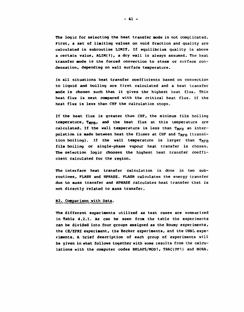
- 61 -
The logic for selecting the heat transfer node is not complicated.
First, a set of limiting values on void fraction and quality are
calculated in subroutine LIMIT. If equilibrium quality is above
a certain value, ALIM(1), a dry wall is always assumed. The heat
transfer mode is the forced convection to steam or surface con
densation, depending on wall surface temperature.
In all situations heat transfer coefficients based on convection
to liquid and boiling are first calculated and a heat transfer
•ode is chosen such that it gives the highest heat flux. This
heat flux is next compared with the critical heat flux. If the
heat flux is less than CHF the calculation stops.
If the heat flux is greater than CHF, the minimum film boiling
temperature, TRPB, and the heat flux at this temperature are
calculated. If the wall temperature is less than T^FB an inter
polation is made between heat the fluxes at CHF and T^FB (transi
tion boiling). If the wall temperature is larger than T^PB
film boiling or single-phase vapour heat transfer is chosen.
The selection logic chooses the highest heat transfer coeffi
cient calculated for the region.
The interface heat transfer calculation is done in two sub
routines, FLASH and HPHASE. FLASH calculates the energy transfer
due to mass transfer and HPHASE calculates heat transfer that is
not directly related to mass transfer.
B2. Comparison with Data.
The different experiments utilized as test cases are summarized
in Table 4.2.1. As can be seen from the table the experiments
can be divided into four groups assigned as the Roumy experiments,
the CE/EPRI experiment, the Becker experiments, and the ORNL expe
riments. A brief description of each group of experiments will
be given in what follows together with some results from the calcu
lations with the computer codes RELAP5/M0D1, TRAC(PFI) and NORA.
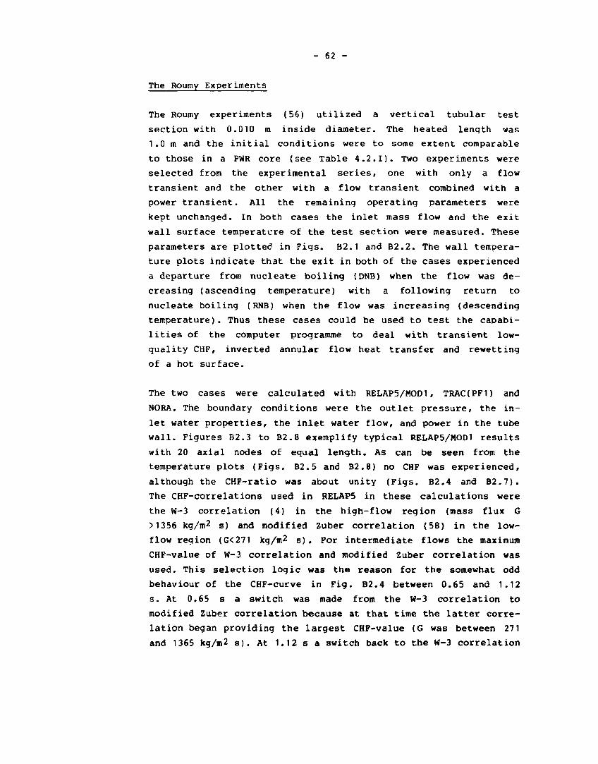
- 62 -
The Roumy Experiments
The Roumy experiments (56) utilized a vertical tubular test
section with 0.010 m inside diameter. The heated length was
1.0 m and the initial conditions were to some extent comparable
to those in a PWR core (see Table 4.2.1). Two experiments were
selected from the experimental series, one with only a flow
transient and the other with a flow transient combined with a
power transient. All the remaining operating parameters were
kept unchanged. In both cases the inlet mass flow and the exit
wall surface temperature of the test section were measured. These
parameters are plotted in Figs. B2.1 and B2.2. The wall tempera
ture plots indicate that the exit in both of the cases experienced
a departure from nucleate boiling (DNB) when the flow was de
creasing (ascending temperature) with a following return to
nucleate boiling (RNB) when the flow was increasing (descending
temperature). Thus these cases could be used to test the capabi
lities of the computer programme to deal with transient low-
quality CHF, inverted annular flow heat transfer and rewetting
of a hot surface.
The two cases were calculated with RELAP5/MOD1, TRAC(PFI) and
NORA. The boundary conditions were the outlet pressure, the in
let water properties, the inlet water flow, and power in the tube
wall. Figures B2.3 to B2.8 exemplify typical RELAP5/MOD1 results
with 20 axial nodes of equal length. As can be seen from the
temperature plots (Figs. B2.5 and B2.8) no CHF was experienced,
although the CHF-ratio was about unity (Figs. B2.4 and B2.7).
The CHF-correlations used in RELAP5 in these calculations were
the W-3 correlation (4) in the high-flow region (mass flux G
> 1356 kg/m2 s) and modified Zuber correlation (58) in the low-
flow region (G<271 kg/m2 s). For intermediate flows the maximum
CHF-value of W-3 correlation and modified Zuber correlation was
used. This selection logic was the reason for the somewhat odd
behaviour of the CHF-curve in Fig. B2.4 between 0.65 and 1.12
s. At 0.65 s a switch was made from the W-3 correlation to
modified Zuber correlation because at that time the latter corre
lation began providing the largest CHF-value (G was between 271
and 1365 kg/m2 s). At 1.12 s a switch back to the W-3 correlation
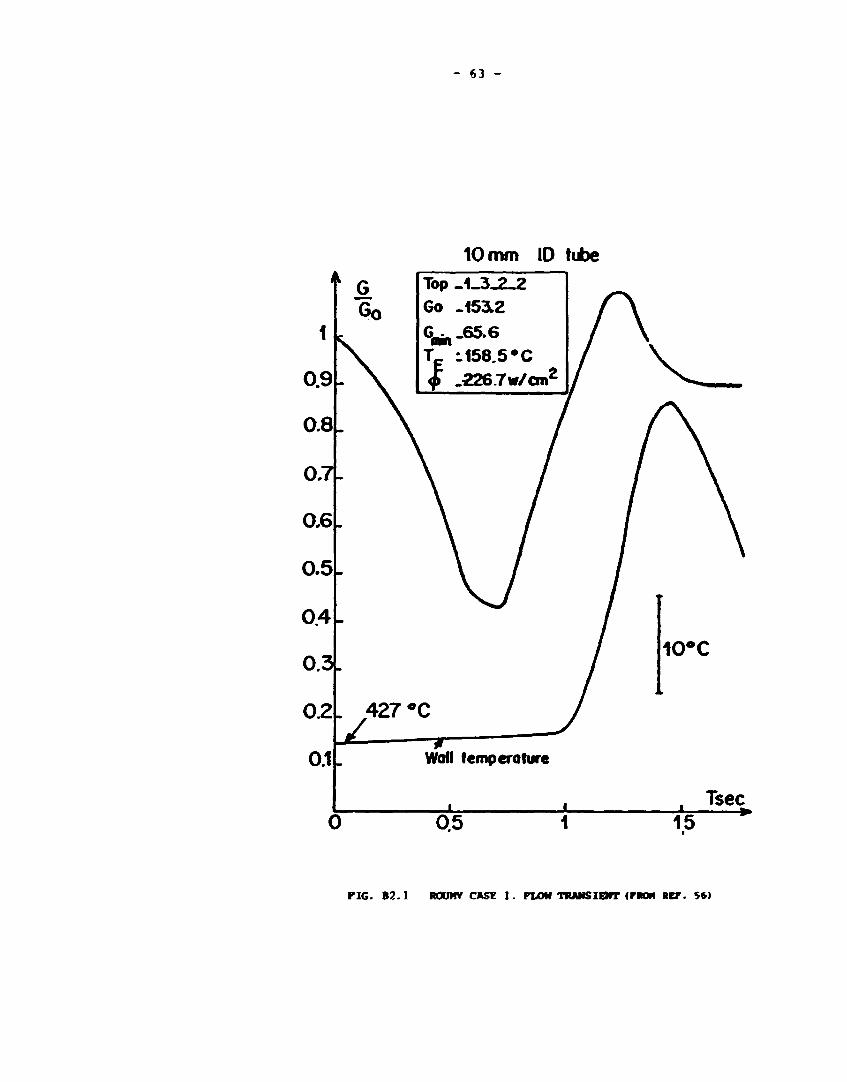
- 63 -
10 mm ID tube
FIG. B 2 . 1 ROUMV CASE ] . FLOW TRANSIENT (PMOM BET. $61
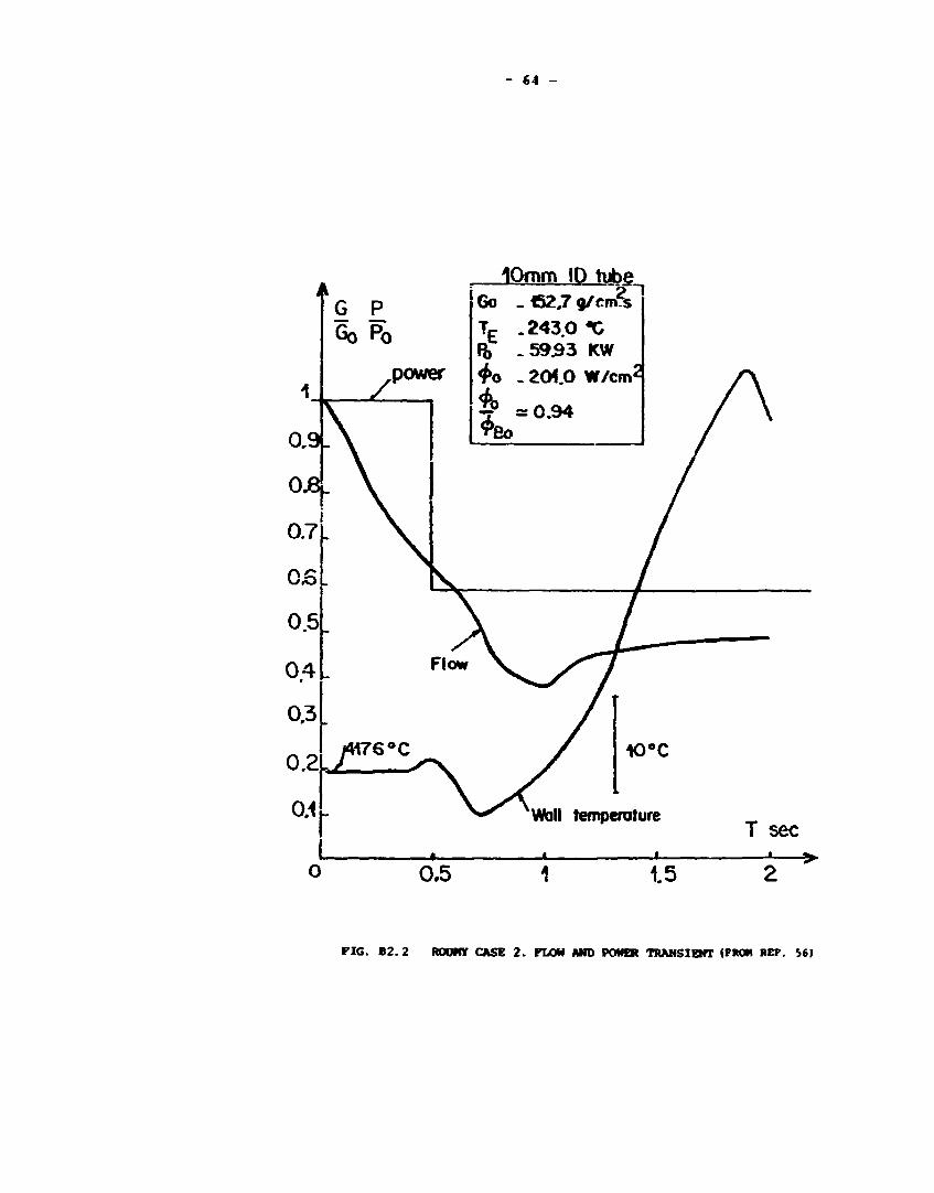
- 64 -
10mm ID tube
G £ Go Po
power
0,9.
0.8. i
0.7
QB
0.5
04 »
0.3
0.2
Go
\ *
* o
- C2.7 g/cm?s .243.0 *C _59j93 KW . 204.0 W/cm2
= 0.94
Flow
/ H76°C
0.4
10°C
Wall temperature T sec
0.5 1.5
PIG. B2.2 ROUMY CASE 2. FLOW AND POWER TRANSIENT (PROM REP. S6)

- 65 -
• i «
.U _
o
« 01
i
.14
.12
.10
.08
• 0t
*• 9 • • •
.04
.02
X JL _L _L X X X J 0.00
5-0 r-
0.25 0.50 0.75 1.00 1.2S 1.50 1.7S 2.00
T I M E (SEC)
Fig. B2.3 REIAP5/MOD1/018 Roumy Case 1
Biasi
z
u
4.5
4.0 R-
3.5
3.0
2.5
• 2.0
Si 1-5
1.0
0.5
Heat Flux
CHF observed in test
i JL X X X _!_ X 0.00 0.25 0.S0 0.75 1.00 1.25 1.50 1.75
T I M E ( S E C )
Fig. B2.4 RELAP5/MOD1/018 Roumy Case 1
2.00
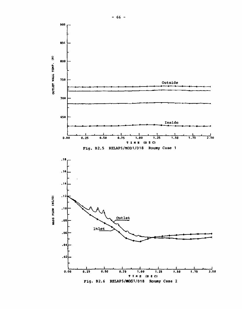
- 66 -
900 l—
esc
800 —
o.
5 j
J 750
8
Outside i i i < « i i 1 1 < « — — « < • • • • •-: i 1 1
700
6S0
Inside
o.oo .i I • L
0.25 X J_ _L J_ _L
0 . 5 0 0 .75 1 .00 1 .25 1 .50 1 .75
T I M E ( S E C )
F i g . B2.5 RELAP5/MOD1/018 Roumy Case 1
i 2.00
U.
(A
-18,—
. 1 6
.14
.12
.10
.08
. 06
.04
.02
J u JL ± _L 0.00 0 . 2 5 0.50 0 .7S 1 .00 1 .25
T I M E ( S E C )
F i g . B2.6 RELAP5/H0IJ.1/018 Rouiny Case 2
1.50 1.75 2.00

- 67 -
5.0
4 .5
4 .0
X
X
u
X o z < X
u
3.5
3.0).
2 .5
2 .0
1.5
1.0
0.5 -
! X J . _L J_ _L J 0.00 0.25 0.50 0.75 1.00 1.25
T I M E ( S E C )
F i g . B 2 . 7 RELAP5/MOD1/018 Roumy C a s e 2
1.50 1.75 2.00
900 __
850 _
* 600
i 750
700
650
*- » » » ii o » . Inside * * * • • • • • » > » « » » «
0.00 J .
0.25 0.50 _L J_ l
0.7S 1.00 1.2S T I M E ( S E C )
F i g . B2.8 RELAP5/MOD1/018 Roumy Case 2
1.50 1.75 2.00
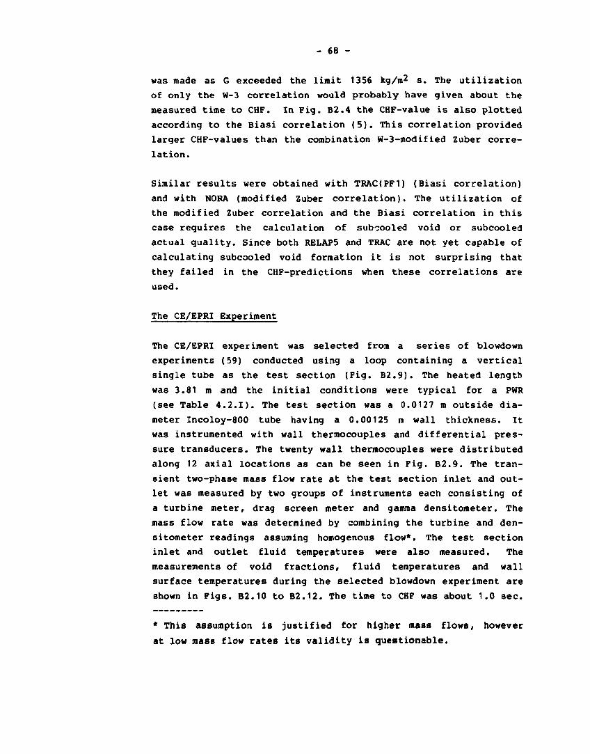
- 68 -
was made as G exceeded the limit 1356 kg/m2 s. The utilization
of only the W-3 correlation would probably have given about the
measured time to CHF. In Fig. B2.4 the CHF-value is also plotted
according to the Biasi correlation (5). This correlation provided
larger CHF-values than the combination W-3-modified Zuber corre
lation.
Similar results were obtained with TRAC(PF1) (Biasi correlation)
and with NORA (modified Zuber correlation). The utilization of
the modified Zuber correlation and the Biasi correlation in this
case requires the calculation of subcooled void or subcooled
actual quality. Since both RELAP5 and TRAC are not yet capable of
calculating subcooled void formation it is not surprising that
they failed in the CHF-predictions when these correlations are
used.
The CE/EPRI Experiment
The CE/EPRI experiment was selected from a series of blowdown
experiments (59) conducted using a loop containing a vertical
single tube as the test section (Fig. B2.9). The heated length
was 3.81 m and the initial conditions were typical for a PWR
(see Table 4.2.1). The test section was a 0.0127 m outside dia
meter Incoloy-800 tube having a 0.00125 m wall thickness. It
was instrumented with wall thermocouples and differential pres
sure transducers. The twenty wall thermocouples were distributed
along 12 axial locations as can be seen in Fig. B2.9. The tran
sient two-phase mass flow rate at the test section inlet and out
let was measured by two groups of instruments each consisting of
a turbine meter, drag screen meter and gamma densitometer. The
mass flow rate was determined by combining the turbine and den
sitometer readings assuming homogenous flow*. The test section
inlet and outlet fluid temperatures were also measured. The
measurements of void fractions, fluid temperatures and wall
surface temperatures during the selected blowdown experiment are
shown in Figs. B2.10 to B2.12. The time to CHF was about 1.0 sec.
* This assumption is justified for higher mass flows, however
at low mass flow rates its validity is questionable.

- 69 -
In the calculations with the three computer programmes only the
test section was modelled. Thus some adequate boundary conditions
had to be given. The boundary conditions used in these calcu
lations were the outlet pressure (Pig. B2.13), the inlet massflow
(Fig. B2.14) and the test section power (Fig. B2.15). As the pro
grammes required the phasic massflows the total massflux in Pig.
B2.14 had to be divided on each phase. This was accomplished by
means of Pigs. B2.10 and B2.11 with the assumption of saturated
homogeneous flow.
The results of the RELAP5/M0D1 calculations are shown in Pigs.
B2.16 to B2.19. Similar results were obtained with TRAC(PFI)
and NORA. The exit void fraction in Pig. B2.16 showed about the
same trend as the measured exit void fraction in Pig. B2.10,
being on a somewhat higher level though. The measured exit tem
perature peak shown in Pig. B2.11 was also obtained in the
calculations (Fig. B2.17). The temperature peak occurred somewhat
earlier in the calculations and, significantly, it was predicted
to have a shorter duration, about 1 sec or half of the measured
2-sec duration. In Figs. B2.18 and B2.19 some calculated wall
surface temperatures are shown.
A comparison with the measured temperatures in Pig. B2.12 reveals
an almost correct calculated time to CHF while the rewetting was
predicted to occur too early. A more notable discrepancy was the
prediction of fairly uniform CHF and rewetting throughout the
test section while the measurements indicated an axial propa
gation of the CHP and also of the rewetting.
There could apparently be two reasons for these discrepancies:
first, of course, some inadequacies of the models used in the
programmes, and secondly the utilization of inadequate boundary
conditions. One of these is certainly the assumption of saturated
homogeneous flow when evaluating the phasic flow components
from the measurements.
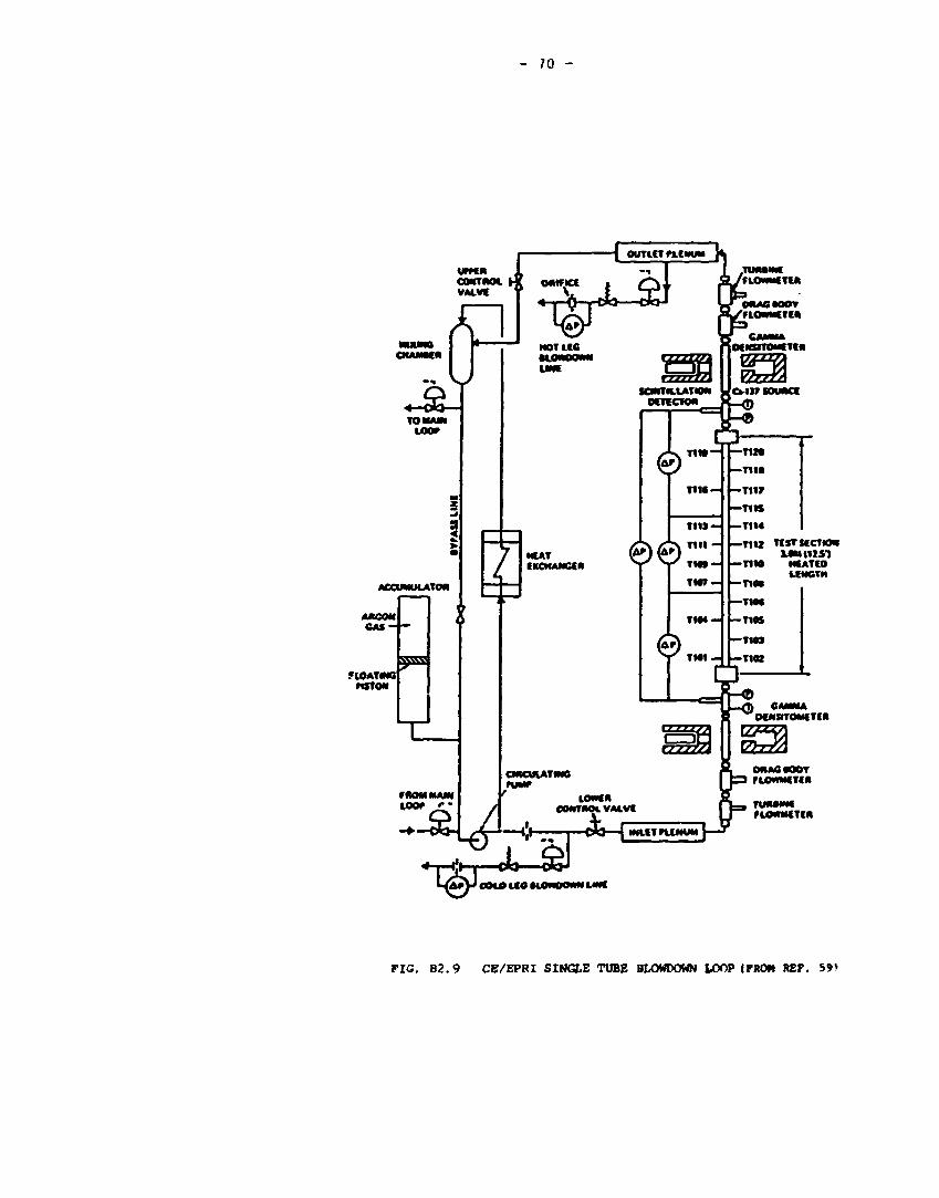
70 -
urret*
OUTUT PLENUM
»"^^JLSt
T
«-øb— TOMAM
toor
ACCUMULATOR
CAS"
nOATWS nSTON
BSS
MOM MAM
toor r
HOT ICC KOM UWE
7 t
MtAT fKCNAMCCa
T I O « -
© TM)I -
— T I « TCSrsCCTKM XMK1151
h-TIIO MEATCD LENGTH
h-TIOJ
— T K *
— T10S
— T I «
—Ties
Kr
CmCUlATMO ruMP
LOWfN VALVE - ' JL / CONTftOL VAU
_ 0 ) CAMMA OfMSITOMCTCft
WUTPUNUM
MAO H O T riOMMCTC«
ruM«Mc flOWKCTtft
> COlO U « MOMKMM LMfC
FIG. B 2 . 9 CE/EPRI SINGLE TUBE SLOWDOWN LOOP (FROM REF. 59>
- 71 -
3 4 S TIME, SECONDS
FIG. 92.io Single cube cranslenc void reactions (PROH REP. 59)
•t 0
350 c °
2 4 6 TIME, SCC0N0S
PIG. B2.ll Single cube cranslenc fluid cemperacures (FROH REP. 59)
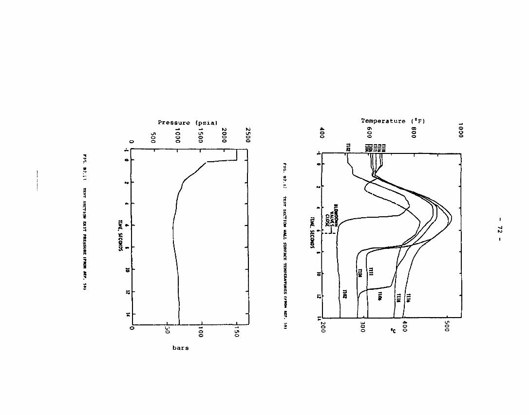
Pressure (psia) Temperature (°F)
\J* o o
—» o o o
—» en o o
Ni O o o
ro Ul o o
3
TE
S
-) SEC
T
i s 3 3 fa s
J h
a r*
S s - s
o o
o o
i si
00 o o
o o o
I
1 1
• J ill :.JJ
.
• §
—Trm—' ' •
]// X
*^ nw
i
2 / /
5 i • I 1.
ISJ
O O
O o
o o
en o o
bars
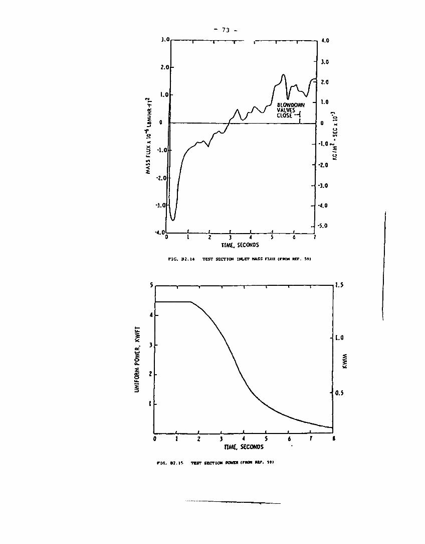
J.O
- 73 -
T r 4.0
2.0-3.0
-4.0
o
JL -S.0
3 1 2 3 4 5 6 TIME. SECOM0S
FIC. B 2 . U TEST SECTION INLET HASS FLUX (FROM »EF. 5»>
3 < 5 nMC. SEC0N0S
*-"-•s \c
m ec £ O au S ae o 1^ i
./
4
1
J
l
-
.
.
•
i
i
•
i i
- >
i
i
i
1
i
i
•
1.5
1.0
I • 0.5
rir,. B2.IS TBST SECTION KWEft (f«0B ««f. *tl
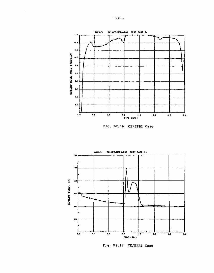
- 74 -
SAEK-5 RCLAtt'tUO-WO-W TEST CASE 3.
O.I
M 0.7
o Si h> 0.«
> O.J
U O g 0.4
g 0.3 S o
0.2
-
• p •
•
•
-
•
-
»
^^\r
» * •
J.O 4.0 TIHE ISEO
F i g . B2 .16 CE/EPRI Case
SAEK-5 RELAPS/nOOI/OIS TCST CASE 3 .
100
s
3 tie
0.0 J.O I.« 4.0
Tine (scci 0.0
F i g . B 2 . 1 7 CE/EPRI Case
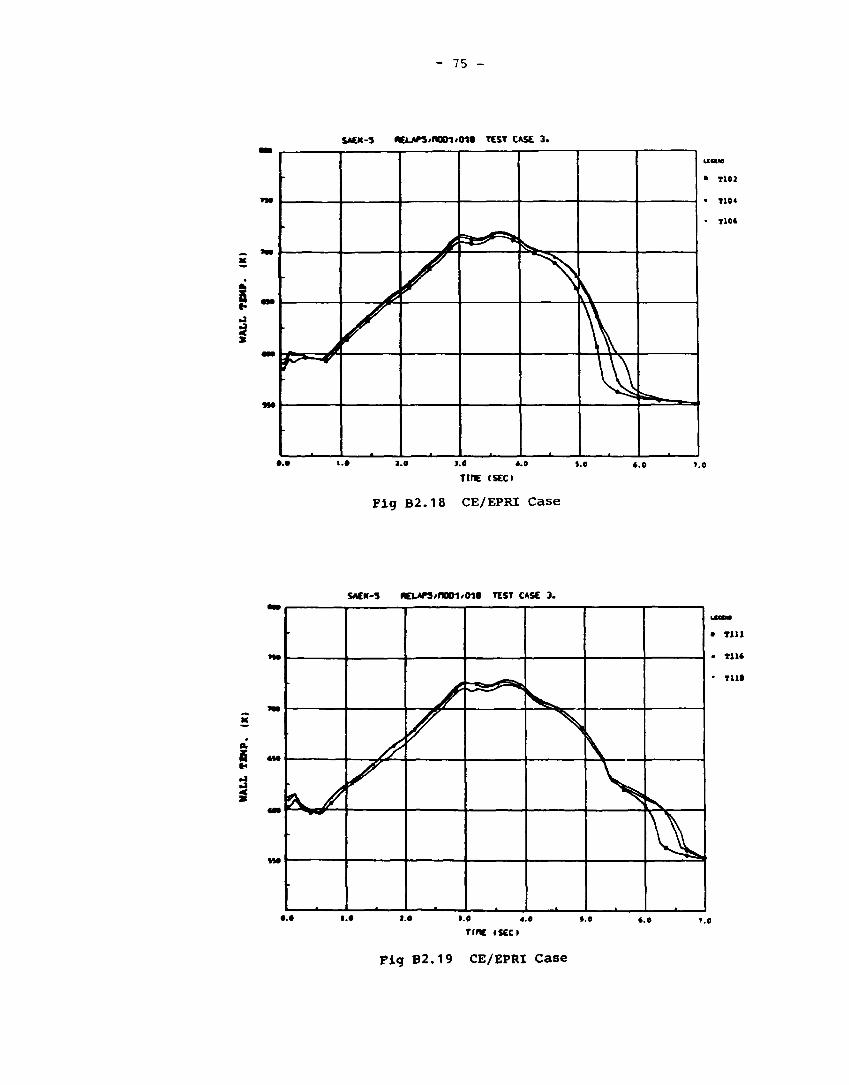
- 75 -
SACK-3 «cu«>nan»oit TEST CASE 3.
fi CS*
9 M
•
j 4
^ r
• TlOJ
• T104
• T104
«.0
TIHE <SEC»
F i g B2 .18 CE/EPRI Case
•n K/
SACK-3 fCLATS/nOOl/010 TEST CASE 3.
/?
• T i l l
• Tilt
• T i l l
1.0 I.« 4.« rine (scc>
P i g B2 .19 CE/EPRI Case
- 76 -
It soon became obvious from the results of the simulations of
the three transient test cases described above that the calcu
lations were influenced by a large number of utilized models and
empirical correlations apart from the applied boundary conditions.
Thus, it would be very difficult to assess the heat transfer
correlations alone from these types of transient experiments.
More simplified experiments were desirable, preferably steady-
state experiments with well-defined boundary conditions. In order
to cover the complete spectrum of heat transfer modes experiments
in which it was desirable to exceed CHP. Two groups of experiments
which met these new requirements were found, the Becker >nd
ORNL experiments.
The Becker Experiments
The Becker experiments were selected from a series of CHF and
post-CHF experiments reported in (2). As the CHF in these ex
periments all were of the annular liquid film dryout type, the
term dryout (DO) will be used henceforth. The test section used
in these experiments was a vertical tube, directly heated in the
tube wall and insulated on the outer surface. The inside diameter
was 0.0149 m and the heated length was 7 isi with an uniform power
distribution. The lower 3 m was instrumented with wall thermo
couples at every 0.25 m and the upper 4 m at every 0.1 m (cf
Fig. B2.20).
The steady-state conditions for the seven selected cases are shown
in Table 4.2.1. The cases were calculated with the computer pro
grammes RELAP5/MOD1, TRAC(PF1) and MORAS (the steady state version
of NORA) and the steady state conditions in Table 4.2.1 were
used as boundary conditions, viz. exit pressure, inlet mass flow,
inlet subcooling and heat flux.
The first calculations of these test cases (or some of the cases)
are reported in (60) to (63). As there were no provisions in
RELAP5 nor in TRAC to calculate the steady state this had to be
done by analyzing a transient with time-invariant boundary con
ditions until the solution was stable. With 20 to 35 axial

- 77 -
nodes the CPU-time on a CDC CYBER 170-835 computer for obtaining
the steady state in these cases ended up in the ranga 10 to 20
minutes while the NORAS programmes required only a few seconds.
For that reason only some of the selected seven cases were calcu
lated with RELAP5 and TRAC while all of them were calculated with
NORAS.
The RELAP5/HOD1 calculations were carried out with two different
CHF-correlations, the w-3 correlation (4) and the Biasi correla
tions (5). In all of the cases using the W-3 correlation the
predicted locus of DO were too far upstream, in the calculations
using the Biasi correlations the high flow DO was due to a cut
off void limit of 0.96. A more thorough examination of these
results revealed that the value of DO too far upstream was caused
by some flow oscillations during the course to steady state in
combination with the incapability of RELAP5 to rewet an initially
dry surface without decreasing the surface temperature, i.e.
without decreasing the power.
The results from the TRAC(PF1) calculations revealed fairly ac
curate DO predictions. TRAC applies the Biasi correlation; however,
in none of the cases did this correlation determine the locus of
DO. Rather, an arbitrarily chosen cutoff void limit of 0.97 caused
DO.
Both RELAP5 and TRAC calculations revealed significant dis
crepancies between predicted and measured wall surface post-DO
temperatures. The post-DO conditions are known to be strongly
dependent on the conditions at the locus of DO. It was therefore
not possible to decide whether wall temperature discrepancies
were due to an erroneous prediction of post-DO heat transfer.
The NORAS calculations (63) used three different CHF-correlations:
Biasi, CISE4 and Becker (64). Biasi and Becker correlations pre
dicted DO as lying too far downstream while, on the other hand, the
CISE4 correlation predicted DO as too far upstream at high quality
and too far downstream at low quality. Calculations were also
performed with either Biasi or CISE4 correlation adjusted by a
factor to obtain predicted DO locations as close as possible to
- 78 -
measured values. This was made in order to obtain a reasonable
comparison between predicted and measured post-DO wall surface
temperatures. The results from these calculations indicated that
the post-DO interfacial heat transfer needed some improvements.
For Becker case 1 the interfacial heat transfer was varied
until a satisfactory agreement between predicted and measured
post-DO temperatures was obtained (Fig. B2.21).
The major conclusions from these calculations were that the DO
predictions in all of the codes needed substantial improvements
and that the post-DO heat transfer calculations needed refine
ments.
Some examinations of the heat transfer package of RELAP5/M0D1
(65,66) revealed that the static equilibrium quality was used as
an input to correlations even though the equilibrium flow quality
was used in the development of the correlations. At the DO
location the vapour velocity may be much higher than that of the
liquid. Consequently, the flow quality will be higher than the
static quality. This means that the use of static quality in a
correlation will result in higher critical heat flux than if the
flow quality was used.
It was also apparent that the interfacial heat transfer was too
high in RELAP5 and TRAC(PFl) and too low in NORA.
In order to examine the post-DO heat transfer calculations in
RELAP5/M0D1 and TRAC(PFl) five of the Becker test cases were
recalculated with the experimental locus of DO given as input
(67,68). To accommodate this new input the RELAP5 and TRAC com
puter programme had to be somewhat modified, especially the in
put routines and the routine performing the CHF calculations.
When the DO locus was inserted, the uncertainties in the DO
predictions were eliminated and the results from the post-DO
heat transfer calculations could be used to examine the pertinent
models and correlations more thoroughly. The results from the
calculations with RELAP5 are shown in Figs. B2.22 to B2.26. The
predicted post-DO wall temperatures were significantly lower than
the measured ones. Moreover, it appeared that the calculations
- 79 -
of the nonequilibrium effects typical for the post-DO regime
were inadequate in that no vapour superheat was calculated (the
liquid and vapour post-DO temperatures we* about the same).
Four cases were recalculated with a test version of RELAP5/M0D 1
in which the post-DO interfacial mass transfer and the post-DO
wall-to-fluid heat tranfer models were completely modified (69).
The vapour phase was now allowed to be superheated when the
quality exceeded the quality at DO rather than a fixed value*.
In the post-DO region the vapour generation rate was calculated
from a new correlation (6) and the wall heat transfer was assumed
to take place from the wall surface to the superheated vapour
phase only. The predicted wall temperature distributions in the
post-DO region showed substantial improvements compared to the
earlier calculations (Figs. B2.27 to B2.30).
The modifications outlined above had been adopted ealier in
NORAS (70,71) and the Becker cases had been recalculated. The
NORAS calculations then gave about the same temperature distri
butions in the post-DO region as the RELAP5 calculations de
scribed above. The modified NORAS was also used to simulate
some rod bundle experiments conducted at OTJJL. These are dis
cussed below.
* Originally RELAP5 made use of a fixed static quality value
to determine which phase was saturated, if the static quality
was less than 0.5 the vapour phase was saturated; otherwise
the liquid phase was saturated. The phase that was unsaturated
was allowed to be either subcooled or superheated.
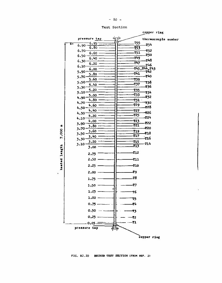
- 30 -
Test Section
pressure tap
6.95
pressure tap
T42
copper ring
thermocouple number
copper ring
FIG. B2.20 BECKER TEST SECTION (FROM REF. 21
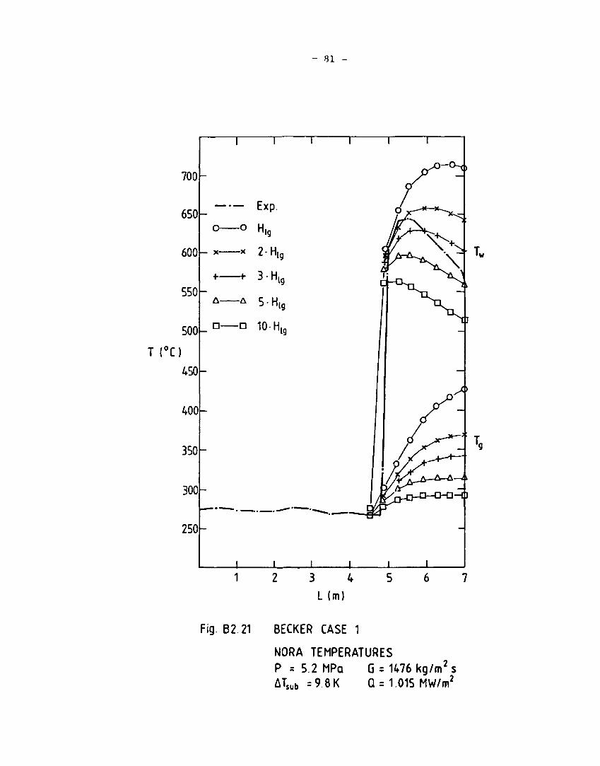
- 31 -
T (°C)
700
650
600
550
500
)
450
400
350
300
250
Exp.
o o H lg
h-x x 2 H
+ h 3 H
ig
19
-A 5 H (g
-D 10 H ig
± 1 2 3 4 5
L im)
Fig. B2.21 BECKER CASE 1
NORA TEMPERATURES
P = 5.2 MPa ATsub =9 8K
G = 1476 kg/m' s Q = 1.015 MW/m2

82
SAEK-5 RtLAP5/nODl/019 BECKER CASE 1,
CO LU
o
LU
a. <
o
o. i-UJ 1--_I _J <
TiO.
100.
650.
eoo.
V50.
SCO.
^ -.so.
400.
JSO.
JOO.
zso.
200.
-
-
-
-
-
-
-
-
-
^ "* •
1 1
WALL
r^ L
E X P E R I M E N T A L DATA
r>
T E M P E R A T U R E
.TOfTTn TF
V A P O R TEM
I , 1
" ""
i
' • - e b,
2MPERATL
V
i;-^J PERATtJRR /
i '
\ \
\
1 0. J. i..
LENGTH (Cl)
FIGURE B2.22
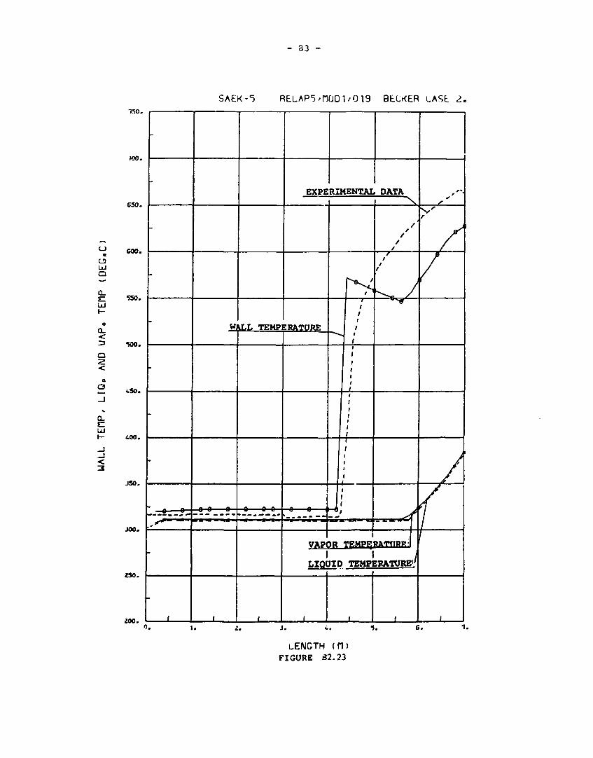
- 33 -
SAEK-5 RELAP5>ri001/019 BELKER LÅSE 2.
o a
UJ
o
LU
OL
<
o _1
Q_
LU
150.
røo.
650.
600.
550.
500.
<.S0.
£00.
J50.
J00.
250.
-
-
-
-
-
-
-
-
• - e »-,*+- —
-
'
Jfl
- « - e — o -
'
U,L TEMPI
-« e-e-
i
EXPERIMENTAL
SRATURE
— 8 8 1 >—i
- • - — - " »
VAPOI 1
LIQU1
'
S o /
/
J/
i_ ,
i ,
. DATA \
/ /
/ /
• / / / /
i
* TBMPRp a T n R P : ;
1 1 ID TEMPERATURE'/
i l
•
r
i
,'*
>y
0. 5. 6 .
LENGTH ( f l ) FIGURE B2.23
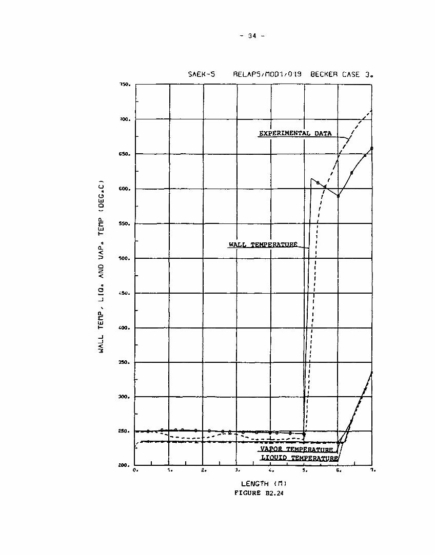
- 34 -
SAEK-5 RELAP5/H0D1/0 19 BECKER CASE 3. 150.
?00.
650.
600.
550.
500.
Z. iSO.
£00.
330.
300.
250.
200.
-
-
-
-
-
-
-
-
-
1 1
EXPERIMENTAL DATA
WAT.T. TEMPERATURE
r~* "~
1_
"- 1 M » * - — i , '
1 '
/ /
i
(
VAPOR TEMpflRATflRR , L I Q U I D TEMPERATlfRE
1 L L l
* * s s
• /
' /"
/
/
l 7 / ' i
0. 1. z. J. <.. 5.
LENGTH (H) FIGURE B2.24
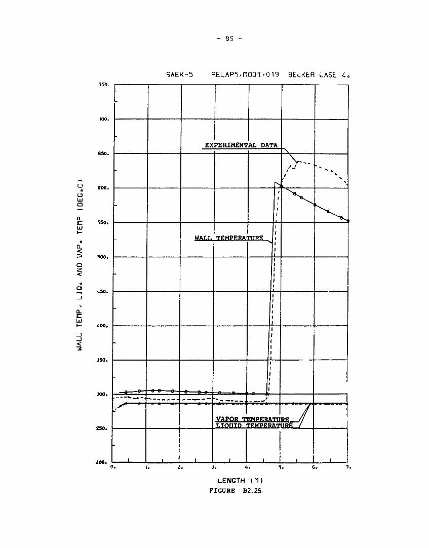
- 85 -
SAEK-5 RELAP^/HODl/OIS BEoKLR CASE c,
irso.
100.
650.
GOO.
550.
500.
r: •.».
<-O0.
JSO.
JOO.
290 .
200 .
-
-
-
-
-
-
-
-
- e o-
,
—e-e e-
.1 -.
EXPERIMENTAL DAT;
WALL
—0 o n
. , , . . .» , .,
r
TEMPERATURE li
!
VAPOR TEMPERAT
i ~ " \ v.. i - N -
i
flRR . // T.TOriTn TEMPERATURE /
J i
*
I 1
"* -s,
V
1
,_„ l , 0 . i . <.. G.
LENGTH (H)
FIGURE B2.25
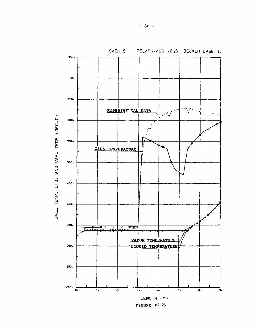
- 36 -
5AEK-5 RELAP5/I10D1/01S BECKER CASE '7, 150.
»00.
650.
GOO.
550.
500.
I I 450.
uOO.
J50.
300.
250.
- - ; * • = * -
£00.
_ZA£OB TEMPERATORE
-LIQVIP TEMJBRÅTURS
J L 0 . 3. G.
LENGTH ,TI)
FIGURE B2.26
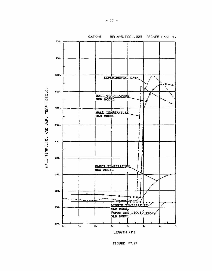
- 37 -
SAEK-5 RELAP5/H0D1/025 BECKER CASE 1, 150.
100.
630.
600.
550 .
500 .
~ 450.
400 .
JSO.
300.
230 .
200.
-
-
-
-
-
-
-
-
-
1
* ^ «*i *w l
l.
EXPERIMENTAL DATA
r WALL TEMPERATURE NEW MODI X
WALL TEMPERATUR! OLD MODE
VAPOR TE UEW MODE
^ *-• ••"•«•. •
:L
MPERATUF L
' a ,
LIQUID T
*̂-*̂_ I
i
i i
—li, r-- * / EMPERATtl }s&y
NEW MODEL § , VAPOR AND LIOUID TEMP/ OLD MODEL
, 1 , 1 , 1 ,
\
1 0 . 1 . 3 . * . S.
LENGTH (H)
6.
FIGURE B2.27

83 -
SAEK-5 RELAP5/11001/025 BECKER CASE 2 .
ej LU o
LU
Q.
<
150.
100.
650.
600.
550.
500.
M tSO.
Q.
LU
< 3
400.
J50.
JO0.
« 0 .
200. 3. * . 5 .
LENGTH <n>
FIGURE B2.28

- 39 -
SAEK-5 RELAP5/n001/025 BECKER CASE 3. •no.
UJ O
OL
o. < o <
•
o
OL C UJ
- I
< 3
J . t . *,.
LENGTH ( f l )
FIGURE B2.29
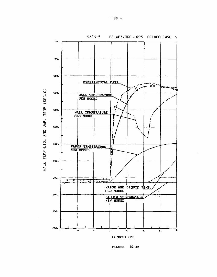
- 90 -
SAEK-5 RELAP5/n001/025 BECKER CASE U
u Q
O (Al Q
ui
o. < a <
ISO.
100.
650.
600.
550.
500.
Zl tSO.
a.
_J < 3
400.
J50.
JOO.
UO.
ioo.
VAPOR AND LIQUID TEMP. OLD MODEL
J 1 v. LIQUID TEMPERATURE^ NEW MODEL
*.
LENGTH (d )
FIGURE B2.30
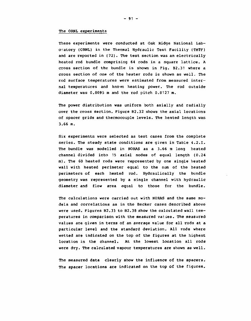
- 91 -
The ORNL experiments
These experiments were conducted at Oak Ridge National Lab
oratory (ORNL) in the Thermal Hydraulic Test Facility (THTF)
and are reported in (72). The test section was an electrically
heated rod bundle comprising 64 rods in a square lattice. A
cross section of the bundle is shown in Fig. B2.31 where a
cross section of one of the heater rods is shown as well. The
rod surface temperatures were estimated from measured inter
nal temperatures and knovn heating power. The rod outside
diameter was 0.0095 m and the rod pitch 0.0127 m.
The power distribution was uniform both axially and radially
over the cross section. Figure B2.32 shows the axial locations
of spacer grids and thermocouple levels. The heated length was
3.66 m.
Six experiments were selected as test cases from the complete
series. The steady state conditions are given in Table 4.2.1.
The bundle was modelled in NORAS as a 3.66 m long heated
channel divided into 15 axial nodes of equal length (0.24
m). The 60 heated rods were represented by one single heated
wall with heated perimeter equal to the sum of the heated
perimeters of each heated rod. Hydraulically the bundle
geometry was represented by a single channel with hydraulic
diameter and flow area equal to those for the bundle.
The calculations were carried out with NORAS and the same mo
dels and correlations as in the Becker cases described above
were used. Figures B2.33 to B2.38 show the calculated wall tem
peratures in comparison with the measured values. The measured
values are given in terms of an average value for all rods at a
particular level and the standard deviation. All rods where
wetted are indicated on the top of the figures at the highest
location in the channel. At the lowest location all rods
were dry. The calculated vapour temperatures are shown as well.
The measured data clearly show the influence of the spacers.
The spacer locations are indicated on the top of the figures.
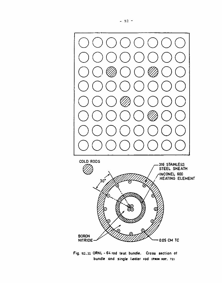
- 92 -
oooo oooo oo#o oooo ooo# oooo oooo oooo
oooo oooo o#oo oooo oooo 0#00 oooo oooo
COLD RODS 316 STAINLESS STEEL SHEATH
HNCONEL 600 ' HEATING ELEMENT
BORON NITRIDE 0.05 CM TC
Fig. 82.31 ORNL -64 rod test bundle. Cross section ot bundle and single Neater rod (FROM REP. 72)
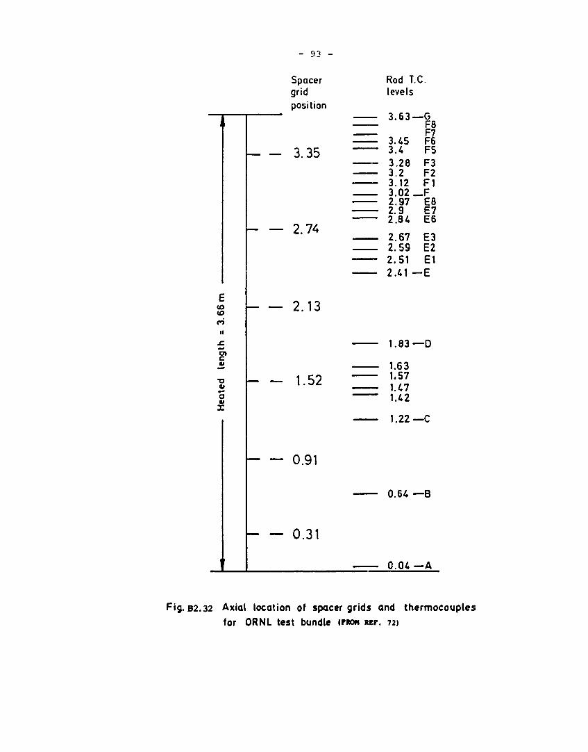
- 93 -
Spacer grid position
Rod T levels
c.
3.35
2.74
CO CO
ri ii
JC
en c a*
TO 41 ** O a* X
— 2.13
1.52
0.91
0.31
3.63 — G F8
45 4 .28 .2 .12 .02
2.97 2.9 2.84 2.67 2.59 2.51 2.41 —
F5 F3 F2 F1
-F E8 E7 E6
E3 E2 E1 E
1.83—D
1.63 1.57 1.47 1.42
1.22—C
0.64 —8
0.04—A
Fig. B2.32 Axial location of spacer grids and thermocouples for ORNL test bundle (FROM REF. 72}
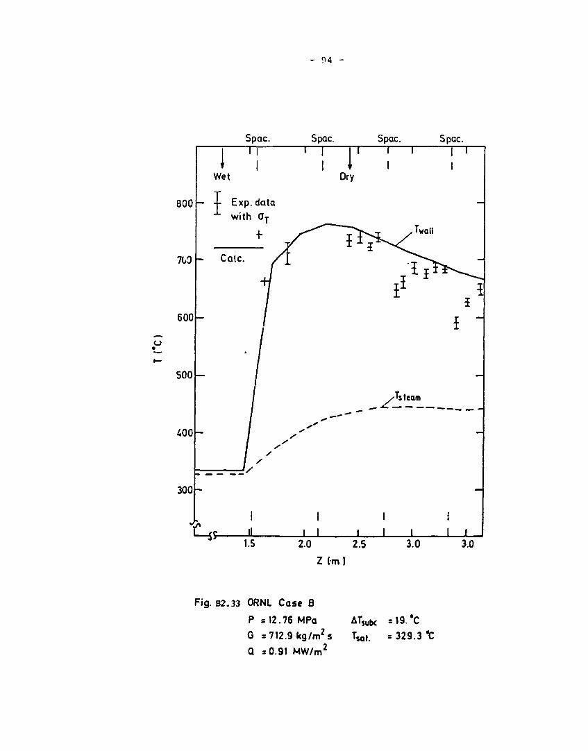
- 94 -
800 h
o
Fig. B2.33 ORNL Case B
P s 12.76 MPa
G =712.9 kg/mzs
Q =0.91 MW/m2
ATjubc = 19. *C W = 329.3 *C
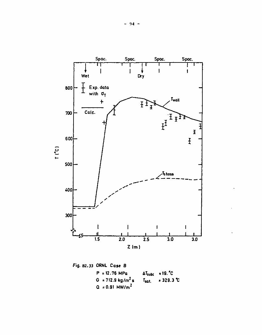
- 94 -
Fig. B2.33 ORNL Case B
P s 12.76 MPa
G = 712.9 kg/m2 s
Q * 0.91 MW/m2
AT$ubc «19.#C W . * 329.3 t
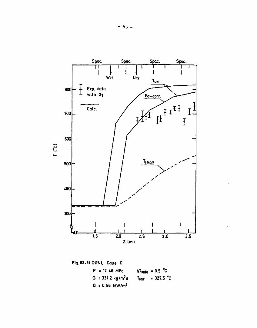
- *»5 -
Spac.
BOO
700
-i
600
500
400
300
k*-
Exp. data with Øj
Calc.
I J I L J L
1.5 2.0 2.5. Z (m)
3.0 3.5
Fig. B2.34 0RNL Case C
P = 12.46 MPa
G s334.2kg/m2s
Q s 0.56 MW/m2
AT$Ub£ s 3.5 C
T,at * 327.5 *C
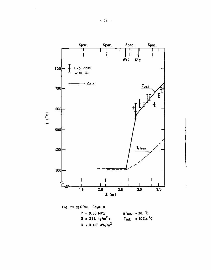
- 96 -
800 h
700
600
500
400 h-
300
I
Spac. T I
Exp. data with 0T
Spac. ""I
I
4S-
Calc.
Spac.
TTJ Wet Ory
Spac. "~TT
I I I I I I I I I L
1.5 2.0 2.5 Z (m)
3.0 3.5
Fig. B2.35 OR NL Case H
P s 8.66 MPa
6 * 256. kg/m2 s
Q = 0.417 MW/m2
ATsubc * 38. C
Tsot. * 302.4 #C
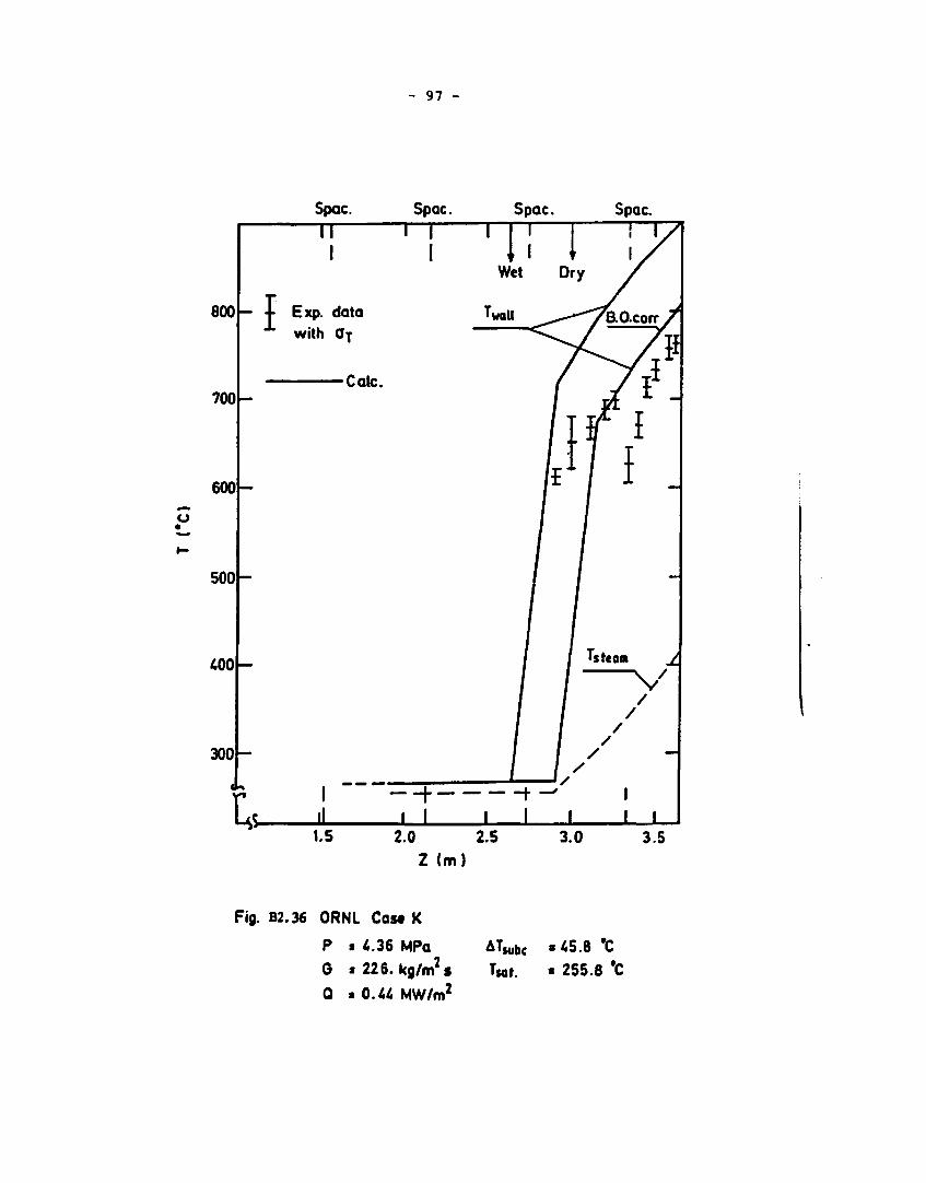
- 97 -
300H
Spac.
TT"
Exp. data with Øj
Fig. B2.36 ORNL C a * K
P • 4.36 MPa G » 226. kg/m2s
0 .O.WMW/m2
ATubc »45.8 'C T$at. * 255.8 'C

- 98 -
Fig. B2.370RNL Case N
P » 8.52 MPa
G * 806. kg/m2s
Q * 0.94 MW/m2
AT«,* «15. *C
T$ot . 300 *C

- 99 -
S pac. Spac. Spac. Spac. TT
Exp. data with Oj
TT ITT Wet Dry
800- I
700-
6 0 0 -
500
400
300-
-4f-
Ca(c.
I J-JL
1.5 2.0 2.5 3.0 3.5 Z (m)
Fig. B2.38 0RNL Cast O
P s 5.98 HPa
G * 307. kg/m2 s
Q » 0.53 MW/m2
A W '22 .3 *C
W • 275.3 *C
- 100 -
Right downstream from a spacer the wall temperature drops due
to flow perturbations induced by it. No spacer effects were
accounted for in the calculations, however.
The locus of DO was predicted using the CISE4 CHP-correla-
tion. Por some of the cases it was considered that the locus
of DC was too far upstreaa and these cases were recalculated
with the locus of the DO moved one node length downstream. These
new wall temperatures are indicated by "BO-corr" in the fig
ures. The results clearly demonstrate the sensitivity of cal
culated wall temperatures to the calculated locus of DO.
B3. Experiences using the computer programmes.
Numerical methods
The work performed in SAK-5 project has mainly been concen
trated on the calculation of steady state tests. Por this pur
pose the numerical method of RELAP5/HOD1 is a semi-implicit
one, which has the maximum tine step of
A tmax< Az/u
where Az is the node length and u is the velocity. In SAK-5
work the maximum time step according to this criteria has been
in some cases less than 5 ms, which leads to excessive computing
time ( ~ 1000-2000 s). If a fully implicit numerical method
could be used, the steady state is obtained using a single
infinitely long time step. In that case the solution method
is iterative and the number of iteration cycles may be large,
but in spite of that the total computation time can be two
orders of magnitude less than it would be using RELAP5.
TRAC(PPI) utilizes a so-called two-step method, which avoids
the stability criteria. A similar method is also used in
RELAP5/MOD 2, which has not been used in this project. Although
the two-step method has no stability criteria, the solution
does not approach the steady state when the size of the time
step is increased. Thus steady state solutions have to be
- 101 -
obtained by transient calculation, which is more time con
suming than the use of a fully implicit method. In order to
calculate the steady state in the test case, TRAC(PFI) re
quired about 200-300 seconds computing time, while the fully
implicit method used in Pinland consumed only 20-30 seconds.
A steady state version of NORA, called NORAS, consumed less
than 10 seconds, but the number of volumes was smaller (20
instead of 35). Furthermore, a direct comparison of the
execution times is not possible, because of different compu
ters, but it seems that TRAC(PP1) consumed at least 10 times
more computing time than a fully implicit method, and RELAP/
MODI about ten times more than TRAC(PPI). The physical assump
tions and spatial discretization methods have also been
different in different computer programmes. RELAP5/HOD1 u-
tilizes only one energy equations. However, this did not
cause any trouble in comparing the calculated results.
All the computer programmes have a conservative discretiza
tion for mass and energy equations. TRAC and RBLAP5 have a
non-conservative form of momentum equations. The results
depend somewhat on which form of the momentum equations is
used, but in the calculated cases the error was not signifi
cant when the node size was 0.2 m. This is natural, because
all consistent numerical methods should have the same solut
ion when the node size approaches zero. With a larger node
size, the difference between a conservative and non-conserva
tive method may be more significant. In the present case
there were also more significant differences in the momentum
fluxes of the individual phases, but the difference in the
total momentum flux was small.
Constitutive equations
Beat transfer correlations are evaluated in a separate Appen
dix; experiences with other constitutive models are shortly
described here. During the work it appeared that many cons
titutive models were not only poorly tested, but they were
also different in different versions of the same computer

- 102 -
programme. An example is the interfacial drag correlation of
RELAP5/MOD1-Cycle 19, which has been applied for the calcu
lations in Finland and Sweden. The programme version used in
Finland has a drag smoothing model, which caused very pecu
liar velocity profiles (see Fig. B3.1).
Another important constitutive model is the one used for
interfacial heat transfer. These models are at present very
simple and crude. In all cases the RELAP-programme predicted
almost equilibrium conditions between the phases. The maximum
temperature difference between the phases was always less
than IK and usually less than O.IK (see Fig. B3.2). It can
be concluded that RELAP5 behaves like an equilibrium computer
programme except in the very early stages of flashing, which
usually occurs only in rapid transients.
There have also been some difficulties in the application of
constitutive equations. Usually the difficulties are caused
by discontinuities in the set of correlation. In RELAP5
these discontinuities have been discovered in interfacial
friction, wall friction and critical heat flux. These are
described in the next chapter.
Difficulties in the application of correlations
The main difficulties in the application of any constitutive
model are caused by discontinuities, when a correlation used
is changed during the calculation. The discontinuities may
prevent convergence of the numerical method and the calcula
ted result is oscillatory. These oscillations also strongly
affect the mass and energy balance and consequently the cal
culated result is unreliable.
In the present work the main difficulties have been caused by
the models of interfacial and wall friction of RELAP5. An
example is the interfacial friction coefficient depicted in
Fig. B3.3. It can be seen that there is a discontinuous change
in the friction coefficient when the void fraction equals
0.65. During the solution, when the void fraction is greater

- 103 -
than 0.65, the friction coefficient has a low value resulting
in a large velocity difference between the phases. This, in
turn, may cause a decrease in void fraction so that on the
next time step or iteration cycle the void fraction is less
than 0.65, which results in a large friction coefficient.
Hence, on the next cycle the velocity difference is again
small and the void fraction is greater than 0.65. Unless a
large amount of numerical damping is added, this oscillatory
cycle goes on forever. When a non-*iterative numerical method is
used like the one of KELAP5, is used this damping can be ob
tained only by the use very small timer steps, which are not
possible in practice.
Another example of numerical difficulties that arise is the
discontinous way wall friction is shared among the phases in
RELAP5.
It is obvious that a constitutive model should not include
computational discontinuities described above, because in
these cases the problem has either no solution at all, or the
solution is obtained only by an ultimately large computational
effort i.e. by using tiny time steps or a large number of
iterations. Because of this a modified wall friction package
has been developed, which has been used for the calculations
of Becker's test cases. In this package the partition of the
wall friction is performed so that the hysteresis phenomenon
is not possible. The results using the new package are nearly
the same as the results of the original package. The new
package results were close to the average of the oscillatory
results, when oscillations occurred in using the original
package. In all cases the total frictional pressure drop in
the channel was the same. Thus the smoothened wall friction
model didnot change the absolute values, but improved the
stability of the calculation,
B4. Comparison using separate programmes
B4.1 Critical heat flux
Due to the difficulties of making an assessment of different

- 104
5(h
40-
30-
Z. 20-o
3 4 5
LENGTH (M) ^ 24.09 i984 T01
Fig.B3.1 Calculated velocity profiles in Becker's test case
no.l. RELAP5/Modl/CYCLE19 in Finland,
RELAP5/Modl/CYCLEl9 in Sweden.
700 _
650
SSO
» »00
4 SO
)S0
100
2J0
200
ISO
1(0
= 120
100
• 0
2«
•
r~
J •j i
•i
J .11 •
<—« •
1 ps
/
/
/
/
/
0.0 1.0 2.0 J.O 4.0 4.0 ( .0 7.0 iXKC'n • A l
Fig. B3.2 Calculated temperatures and vapour generation rate
in Becker's test case No. 1.
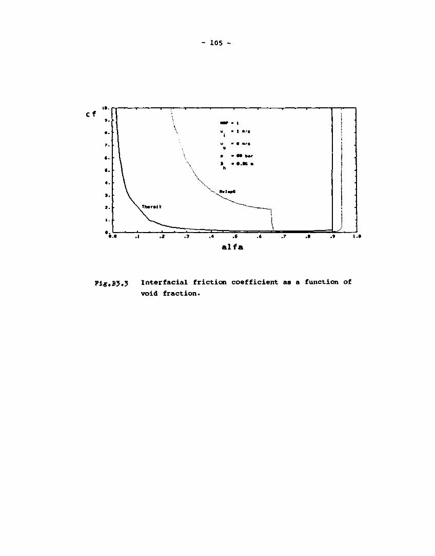
- 105 -
Cf 1 1 • I f
•1 \ • I
• 1
1
• \
\ r h » r « i t
i • i • i » r -
mt - t u - 1 » ' *
1
0
P - « • <f*r
V^««l«»«
^ ^ —
. r • l •
~1 \
"~̂
•
•
t.t .4 .S
alfa
Pig,B3.3 Interfacial friction coefficient as a function of
void fraction.

- 106 -
CHP-correlations employing the thermohydraulic system program
mes like RBLAP5 and TRAC, a separate examination of this issue
was made. The assessment was performed as a separate part of
the SAK-5 project and was conducted at the Royal Institute
of Technology in Stockholm. The result of this assessment is
reported in (73) and in what follows a short summary of the
work will be given. Also some additional efforts made during
the late phase of the project will be reviewed.
The assessment was limited to four different CHF-correlations
and was based on six full-scale steady-state rod bundle experi
ments. The correlations included in the assessment were:
Barnett (74)
Becker (75)
Biasi ( 5)
CISE-4 (76)
The Biasi and CISE-4 correlations were originally developed
for round tubes and thus the performance in rod bundle geo
metries could be questionable. However, as they are utilized
in several of the commonly used transient c<-.nputer programmes,
for instance TRAC(PFI) and RELAP5/N0D1, it was decided also Uo
include those correlations in the assessment. The experimental
data used for this assessment were obtained in a 64-rod bundle
(Desirello et al 77), 81-rod bundle (Pimputkar et al 78), 36-
rod bundle (Nilsson 79 and Nylund 80, 81), and 37-rod bundle
(Bowditch and Smyth 82). These experiments included axially
uniform as well as axially variable heat flux distributions.
The dryout predictions were carried out employing either the
total power hypothesis or the local conditions hypothesis.
In the total power hypothesis the total channel dryout power
was predicted assuming uniform axial heat flux distribution
and compared to the measured power. Thus this method did not
yield any information about the axial location of dryout. In
the local conditions hypothesis, proposed by Becker in 1969
(83), the dryout is assumed to be dependent only on local flow
parameters at the locus of dryout. The principle of this
- 107 -
method is demonstrated in Fig B4.1.1 where the experimental
heat flux is plotted versus the quality along the channel. In
the figure an arbitrary dryout correlation is also included
and the heat balance is represented by a straight line. The
locus of dryout is determined by drawing a family of heat
balance lines for -Afferent axial locations and then selecting
the line yielding '-he minimum value of the ratio (q/A)BOPRE/
(q/A)BOEXP*
Because of the difficulty of defining a proper boiling length
in transient and LOCA situations it is obvious that the
method employing the local conditions hypothesis has to be
adopted for the CHF predictions in these type of transients.
Thus the following will deal only with the results obtained
when using the local conditions hypothesis.
A total number of 269 runs were obtained in the utilized expe
rimental studies mentioned above covering the following para
meter ranges:
Pressure 3.0 - 9.0 NPa
Mass Flux 200 - 2400 kg/in2 s
Inlet Subcooling 12 - 286 kJ/kg
Dryout Heat Flux 0.23 - 1.49 MW/m2
Dryout Steam Quality 0.18 - 0.805
143 of the measurements were obtained with ax i ally non-uniform
ly heated test sections while the remaining 126 measurements
had a uniform axial flux distribution.
Only the Becker and the Biasi correlations covered all the uti
lized experimetal data. Concerning the CISE-4 correlation the
results at pressure 3.0 MPa were outside the range of the cor
relation. Finally the Barnett correlation was valid only for
pressure 7.0 MPa.
The result of the comparison between measurements and predic-
- 108 -
tions can be illustrated by Pigs. B4.1.2 to B4.1.5 showing the
measured versus the predicted dryout power for the 64- and 81-
rod bundles. The .rends for all of the experiments were simi
lar; the Biasi and CISB 4 correlations generally over-predicted
the data considerably while the Barnett and the Becker corre
lations yielded rather good predictions especially for the
square lattice 81, 64 and 36-rod bundles.
A summary of the results obtained with the local condition
hypothesis is shown in Table B4.1.I. The best predictions
were obtained with the Becker correlation yielding a RMS error
of 9.7% including all the runs of the 6 experimental studies.
The Biasi and CISE-4 correlations were in poor agreement with
the experimental data; the reason for this is probably that
these correlations were developed for predictions of dryout
in circular tubes.
Also some selected experiments from the OF-64 experimental
dryout series were analysed (84). This test series was con
ducted by ASEA-ATOM, Sweden, in 1969 and is reported in (85).
The test section was designed as a full-scale simulation of
an Oskarskamn I fuel assembly and consisted of 64 heated rods.
The internal radial power distribution was symmetrical with a
peaking factor of 1.24 while the axial power distribution was
peaked towards the outlet with a peaking factor of 1.55. The
tests were performed with pressures ranging from 4.8 to 8.7
MPa, mass fluxes from 400 to 2000 kg/m2s, and bundle powers
from 5.1 to 8.6 MW. Seven dryout tests were selected for
separate examination and the conditions for these tests
were:
Test No
703007 703073 703015 703075 703077 703087 703043
Pressure (MPa)
6.71 6.82 6.67 6.72 6.82 8.64 4.79
Inlet Subcooling (K)
8.7 7.8 9.4 9.5 9.0 9.2 2.1
Mass Plux (kg/m28)
498 971 1168 1336 1535 1382 789
Power (kW)
5957 7683 7899 8192 8594 6843 7693

- 109 -
In these analyses the Becker and for the 7 NPa cases also the
Barnett correlations revealed the best agreement, while the
Biasi and the CISB-4 correlations were in fairly poor agree
ment with data, i.e. the results were consistent with the find
ings in the assessment reported above. The results obtained
with the Becker correlation is illustrated in Fig. B4.1.6,
indicating a very good agreement although somewhat conservative.
Finally, some predictions of the locus of dryout for the above-
mentioned OF-64 cases were carried out by means of Becker and
Biasi correlations and compared with the measured ones (86).
The conclusions from these calculations were that the Becker
correlation revealed a very good correspondence between pre
dicted and measured locus of dryout for mass fluxes above
1000 kg/ra2 s, the errors being within the measurement accura
cy. For mass fluxes below 1000 kg/m2s the correspondence in
some cases was not quite that good, being on the conservative
side though (the predicted locations were found to be up
stream of the measured ones). It should also be mentioned
that the Biasi CHF correlation? did not predict dryout in
any of the cases, thus being very non-conservative.
B4.2 Transition boiling.
The literature search resulted in the selection of 5
correlations:
1. Chen correlation (29),
2. Correlation by Tong & Young (31),
3. Correlation by Bjornard & Griffith (33),
4. BPRi correlation (87),
5. Correlation by Hsu (32).
The correlations 1, 2, 3 and 5 are shown in Table A3.1.
In 1 and partly also in 2 physical phenomena have been consid
ered to a certain degree. The other correlations may be

- 110 -
64-rod bundle,ref.77
Bl-rod bundle.ref .78
36-rod bundle.ref .79
3S-rod bundle.ref .80
36-rod bundle.ref .81
37-rod bundle.ref .82
Rll Bundles
Barnett
No. of Runs
18
24
11
11
26
69
159
RMS Error
6.5
5.5
15.3
12.2
8.4
11.7
10.3
Becker
No. of Runs
IB
24
18
38
83
88
269
RMS Zrror
11.5
7.0
3.3
10.5
12.5
7.0
"
Biasi
No., of Runs
18
24
18
38
83
88
269
RMS Error
30.7
26.9
20.9
30.3
31.3
34.2
31.2
CISE-4
No. of Runs
16
24
16
32
71
69
230
RMS Error
21.5
16.2
7.9
23.2
22.6
23.2
21.6
TABLE B4.1.I. RMS-ERRORS OBTAINED WITH THE LOCAL
HYPOTHESIS
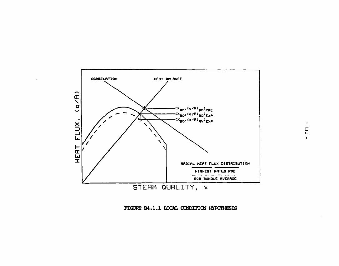
CORRELATION HGRT BflLRNCE
( X B 0 . < q ^ > B 0 ) p R C
( X B 0 . « , ^ R > B 0 ) D ( p
<q'«>, 'EXP
RRDIRL HERT FLUX DISTRIBUTION
HIGHEST RATED ROD
ROD BUNDLE RVERftGE
STERM QUALITY, x
FIGLTRE B 4 . 1 . 1 LOCAL CCNDITTGN HYPOTHESIS
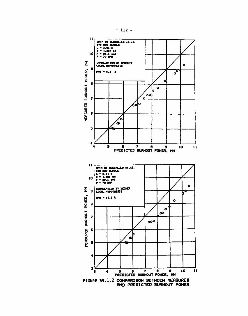
- 112 -
It
10
X J-
- 9 tc u X o a. » B
O z at 3 7 n 7 a ui
I« U S
0HTH IT DCSXMXLO «t .»1 . • • • R00 BUNDLE L - l . l l • 4 - i . n ? • • IT » n . i • • * p - ?o am
COMKLiniON BY BWWCII LOO*. HYPOTHESIS
RHB - C.3 It
/
/ '
/
/ , o
/ oo
1
/ o
tf>
o
5 6 7 8 9 10 PREDICTED BURNOUT POWER, MH
11
£ K U X O
a. 3 o z (E a a
11
10
9
8
7
6
5
4
•J
M m BY oeStMELLO «t.»l • * • MO BUMOLC L - B.tl • * - t . i t r • •
.
P - M . I • • * p - 70 SPR
COMtGLATXOM BY BCCMX LOCH. HYPOTHESIS
RKB - I I . S *
7 /
^
/ >
/
oo°
( o oo
o 1
/
o
r
"3 4 5 6 7 • 9 10 PREDICTED BURNOUT POWER, MM
FIGURE B4.1.2 COMPRRXSON BETWEEN MEASURED RND PREDICTED BURNOUT POWER
I I
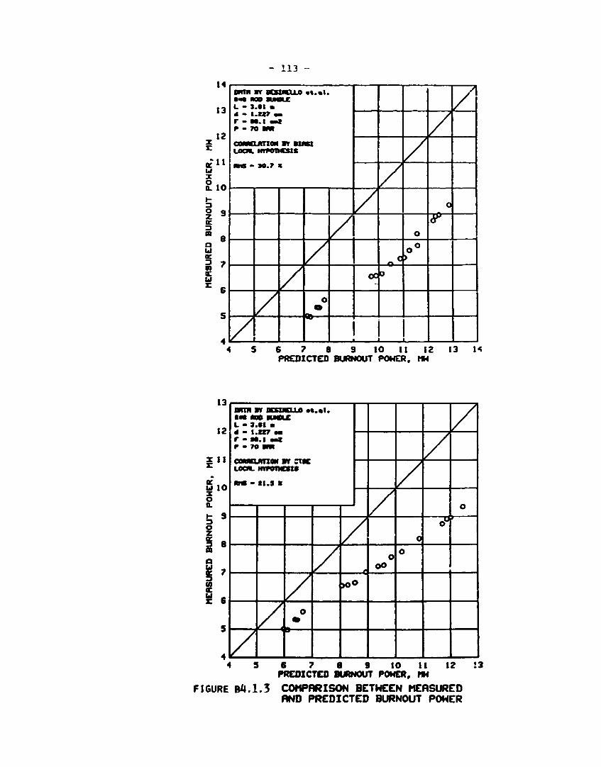
- 113
14
13
12
11
10
9
8
7
6
5
• • * WO BUMLC L - 3.11 m
• t . a l .
4 - I . W w r - M.I H I P - TO BJM
OORMLRTIOM BY B M H LOCH. HYP01MCSK
RMS - M . 7 *
z / /
O
O
G>
oc°
i
O
&
/
6 7 8 9 10 11 12 PREDICTED BURNOUT POWER, MM
13 14
u
13
12
11
10
9
8
7
6
S
mm ir utuiguo •*.•!. • M ROB BUMLE L - J . « l •
r - M.I v i p - 70 am
COMELMlOri BY CUC
IB* - tl.S *
Z /
o
/
£
*>o
/
o oo
/
0
o
/
ou
/
o
4 5 6 7 S 9 10 I I 12 PREDICTED BURNOUT POWER, MH
FIGURE B4.1.3 COMPARISON BETWEEN MEASURED AND PREDICTED BURNOUT POWER
!3
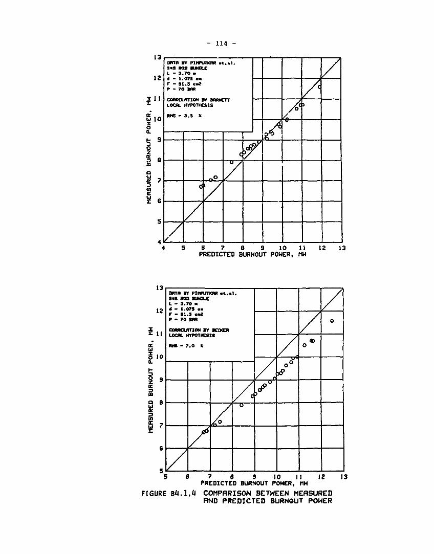
- 114 -
13
12
V1
U 10 o o. y- 9 3 o z 5 e n a « 7 3 (A (C
£ 6
ORTR av piMnnww »t.»i. 9«9 ROD BUNDLE L - 3.70 >
r - 91.3 » 2 P - 70 BUR
coMcurriON BY BWRNCTT
LOCRL HVPOTHCSIS
RMS - 5 .5 K
d O ° J » /
. <
7 /
/ t
6 7 8 9 10 11 PREDICTED BURNOUT POWER, KH
12 13
13
12
z r l i
æ u o 10 o.
3 Z 8
o: 3 n Q B ui te 3 in UI 7
DBTH mr PIMPUTKR« « t . » 9*9 ROD BUHXC L - 3.70 • é - 1.07S en r - st.s cmz P - 70 BR*
CORRELATION >Y KCKER LOCK, KTPOTHESIS
Rns - 7.0 x
/
/ o
c
/ r
>
/ . r o*
0°
/ OD
O
/
O
6 12 7 8 9 10 11 PREDICTED BURNOUT POWER, HH
FIGURE B4.1.4 COMPARISON BETWEEN MEASURED AND PREDICTED BURNOUT POWER
13
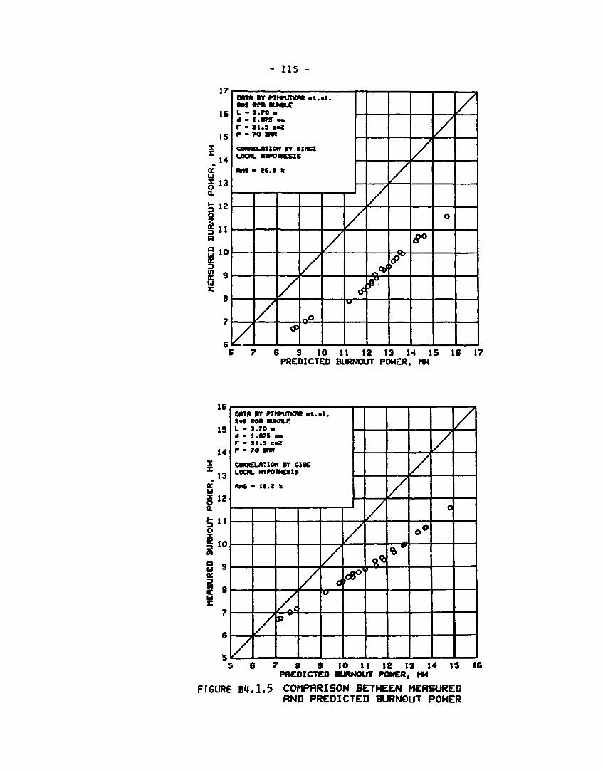
115 -
17
16
IS
r , H
a u S * 3
a. 12 » -
3 O
In GO
S io a; 3 in o U JZ
8
mm rr PXMPUTWM «t. • • 3 ROD BUKKX L - 3 .70 •
k l .
4 - LOTS M I r - S U S ami P - 70 WW
CORRELATION BY I M S I LOCK. HYPOTHESIS
NHS - « . t K
z / /
CP
/
o°
/
^ s V
C?°
O
8 S 10 I I 12 13 14 15 PREDICTED BURNOUT POHER. MH
16 17
16
15
14
£ . I 3
K U
a. 11 3
O
§10 a a 9 U s
K 3
id £
MTA sv pxnninaM »*.»i. •US ROD WNOIX U - 3 .70 • 4 • I .07S en r - 31 .3 ca« P - 70 BMR
CORRELATION I T CISC LOCAL HYPOTHESIS
Mrs - i t . 2 *
z / 4 9
/
/
d V
* > . * * » "
* *
o°
/
0
/
6 7 8 9 10 11 12 13 14 PRCDXCTCO BURNOUT POHCR, MH
FIGURE B4.1.5 COMPARISON BETWEEN MEASURED RND PREDICTED BURNOUT POHER
IS 16

- 116 -
1800 •
—
oil 600 • 3
X
i 1400
HEA
T
£1200 ec
< xiooo
800
O /
£-—t 1
X
/i-
a
— i —
v
•
0
o X
•1-
LEGENO
703007
703015
703011
703073
70307S
703077
703087
800 1000 1200 1400 1600 1800
PREDICTED HEAT FLUX (KW/V)
Figure B4.1.6 OF - 64. Comparison between Measured
and predicted dry-out heat flux.
- 117 -
described as empirical correlations. All correlations are of
the two-term type.
A detailed description of the correlations is given in (26).
A literature search was made in order to find relevant tempera
ture controlled test data. Very few references were found. The
best and most relevant experimental data were those conducted
by Prof. J. Weisman at University of Cincinnati and published
by Electric Power Research Institute (EPRI)r(87).
The temperature controlled surface is ensured by heating the
boiling water by hot flowing mercury. The water flows up
ward in an annulus and the mercury flowing downward in a cen
ter tube. Measurement of wall and mercury temperatures at sev
eral elevations allows the heat transfer to be determined.
The pressures are from 1 to 4 bar. Mass fluxes used in the eva
luation are from 10 to 36 kg/mfysec and steam qualities from
0.02 to 0.54.
A separate computer programme was written to evaluate the 5
correlations with the stated experimental data as input.
A listing of the computer programme is reproduced in Appendix
B in ref. (26). The final results from the evaluation are re
produced in Appendix A of the same reference.
The Chen correlation is based on experimental data from 8 re
ferences with pressures ranging from 4 to 195 bar, mass fluxes
from 16 to 3000 kg/m2/sec, an<j equilibrium qualities from 0.5
to 1.7.
For some parameters the evaluation is the outside the previ
ous range.
The first evaluations gave large deviations from the EPRI re
sults. Two important parameters in the correlation have been
examined: the thermodynamic nonequilibrium and the liquid
contact area fraction (the decay factor).
- 118 -
Both are empirically determined and based or. the experinental
data mentioned above.
The vapour nay be superheated, i.e. part of the heat fron the
surface has been used to superheat the vapour instead of eva
porating the droplets. The actual vapour quality, XA, is less
than the equilibrium quality, XE.
The heat balance gives the following relation between XA and XE:
XA Hfa w = «fg + Cpv " V I S A T )
There are two unknowns in this equation XA and Tv, the super
heated vapour temperature.
Chen defined a parameter B(P):
XA Ty - TSAT — • 1.0 - B(P) • XB Tw - Tw
and determined B(P) from the experimental data:
0.26 B(P) -
1.15 - (P/Pc) W 5
P is the pressure and Pc is the critical pressure.
B(P) approaches 0.226 when P approaches 0.0, where B(P) should
approach 0.0. Some of the experimental data on which B(P) is
determined make it plausible to infer that B(P) is 0.0 when P
is 0.0. Based only on these data B(P) may be correlated as:
B(P) « 8.1-10"2 +2.0*(P/Pc)-4.0 (P/PC)2
for pressures less than 50 bar (Pigure B4.2.1). The result of
this correction is that there will be vapour at lower pressures
as the BPRI data will be superheated earlier than after the
Chen results, in agreement with EPRI data. The deviation has
however, to be examined in more detail.

- 119 -
Chen used his data bank to determine the decay factor using the
relation:
°.LC - <lVC
The decay factor was correlated with the equation:
PL = exp(- X M T W - T S A T)n),
where X. is a function of void and mass flux.
Chen determined the exponent n to 0.5. This gave too low
values of the heat transfer compared with the EPRI result,
however.
The results from the calculations based on the EPRI data were
therefore substituted in the relation for the decay factor; PL
and the exponent n were determined. The functional relationship
for X was retained. Plot of the exponent n is shown in Pig.
B4.2.2. The data have been correlated by two straight lines.
It cannot be excluded that the strong increase in the exponent
near the critical point is due to an inaccurate determination of
the experimental total heat flux near this point cf. Pigs.
B4.2.3-B4.2.7. Only data above about 40 degrees in the tem
perature difference, Tw -TgAT» should have been taken into
into account.
As mentioned above, all experimental data used by Chen et al.
are above 4 bar and most of them are at high pressure.
This may be one explanation of the small exponent.
Chen et al. do not take interfacial heat transfer into account.
An explanation may be that the B(P)-values after Chen's equa
tion imply that the vapour will not be superheated.
Tong 6 Young published their correlation in 1974. In con
tradiction to Chen et al. they use the nucleate boiling heat
flux at CHP as the boiling term, and a modified single-phase
heat transfer correlation (Dittus-Boelter) for the convection
term (see Table A3.I no.2).

- 120 -
B
0.3
0.2
0.1
0 L 0.1
22.1 0.2
44.2 P/Pc
bar
FIGURE B4.2.1
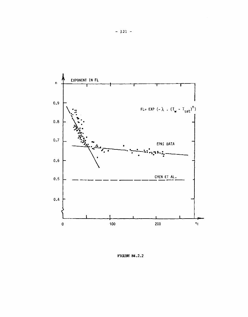
- 121 -
EXPONENT IN FL
T
0.9
0.8
0.7
0.6
0.5
0.4
I
FL=EXP(-X. (Tw-Tsat)")
EPRI DATA
— -sns-;..
CHEN ET AL.
100 200
FIGURE B4.2.2
- 122 -
Tong & Young have used high pressure data to determine the
decay factor. The use of their equation for the decay factor
on the EPRI data gives values that are too high i.e. it is the
boiling term, which is dominant and the correlation will be in
agreement only at low temperature differences near the CHF.
The Tong 6 Young results are not shown in the figures.
The correlation by Bjornard & Griffith (see Table A3. I no.5)
is a purely empirical two-term correlation. The two terms are
defined as the limits between which transition boiling heat
transfer may exist i.e. the critical heat flux and correspond
ing critical temperature, TCHF» a n d the minimum film boiling
heat flux and corresponding temperature, T^pg.
The results of the examination are plotted the Pigs. B4.2.3 -
B4.2.7.
The EPRI correlation is considered because it is developed from
their own experimental results as basis and may therefore
give a first indication of how good are the results.
The above-mentioned correlations are all primarily evaluated
in the vapour-continuous flow region.
The Hsu correlation is developed from subcooled FLECHT data,
i.e. in the liquid-continuous flow region. The results using
EPRI data show a heat transfer that is too high, as may be
expected.
The comparison shows that the description of dispersed flow
with droplets discretely distributed through the continuous
vapour phase and the deposition motion of the droplets toward
the wall is of fundamental importance for the heat transfer
not only in the transition-boiling region, but also partly
in the film-boiling region.
The dividing points between the two regions is the minimum heat
- 123 -
flux, which just represents the point of prevailing droplet wet
collision heat transfer, over heat transferred to the vapour by
convection and droplets entering the thermal boundary layer
withour wetting the surface ("dry" collisions) , and represents
the point of incipient rewetting in emergency core cooling.
The heat transfer using a droplet deposition model may be
divided into, two main questions:
1. How much heat can be carried away every time a
droplet of a certain size impinges and wet the wall?
2. How many droplets per unit time of what size will
penetrate the thermal boundary layer and wet the wall?
Chen et al. inferred a droplet diameter and determined the heat
carried away by "wet" collisions, but did not take "dry"
collisions into account. Nor did they consider the phenomena
under point 2, but determined their liquid contact area frac
tion, the decay factor from the data base they used.
Tong i Young determined their decay factor as covering both
points 1 and 2.
None of the correlations are phenomeno logical in the real
sense of the word.
It is obvious that even some effort has been made to describe
some of the important phenomena, it may be concluded from these
comparisons that the correlations examined in the vapour
continuous flow are valid only within the data base from which
they are developed, i.e. they must still be considered as sta
tistical correlations.

^
I
I—' KJ
t
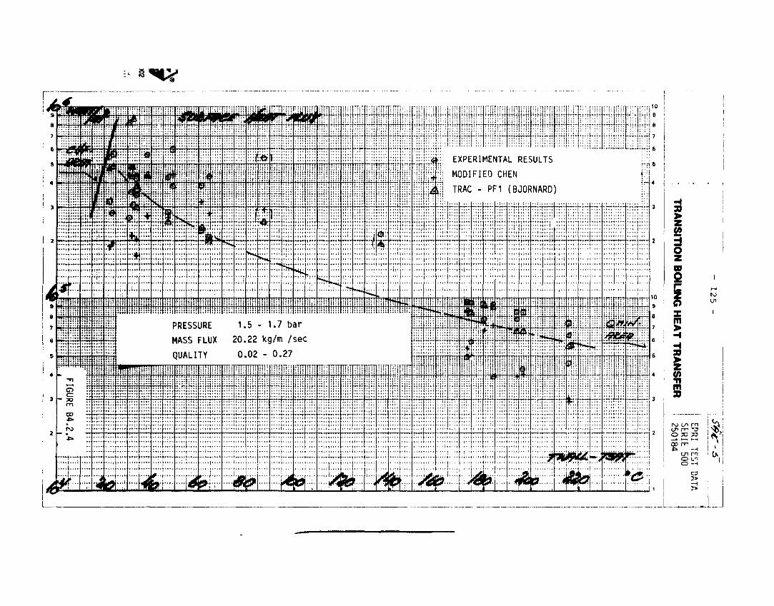
g

* . '
3 > z (O H
5 z OD O
m >
TI m 39
o w m o ^ m "o r o •—i >—< 03 m •fc —i
o m o (/•> o —i
o
at
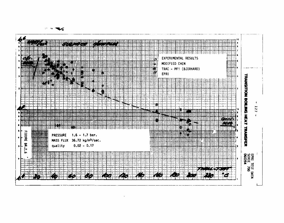
niiiBMMttifft''tr'*triti''"i''f'i""t'Tri'T'-'i''''iittti"'irii'tiLtT',i't',i'iri H^3iii^iLi:J}iWlrø^^ui^l/:!tii<uii^uiiwtø':h..u£ju£HiUu;
liIlli;inii!i!il!!H!ll!!l!li!!il!!linl!i!ill!!f|]!HI!lllllltllllillllllllliyillllililllllllllllltl]ll^
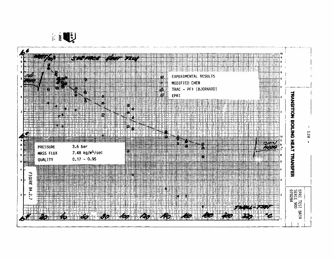
"U>

- 129 -
APPENDIX C. DISPERSED PLOW
CI. Droplet Generation
Droplets are generated partly at all points of the water-vapour
interface in pre-CHF regions due to entrainnent and partly by
sputtering in transition boiling in the post-CHF region.
The droplet generation by entrainaent nay be postulated to take
place in a number of different ways governed by hydrodynamic-
and surface tension forces. (88,10)
Fig. C1.1 shows the various mechanisms.
In the first type the droplets are sheared off from the wave
crests of large-amplitude roll waves. The interfacial friction
deforms the interface against the retaining force of liquid
surface tension.
In the second type the droplets are generated by undercutting
the liquid flow.
In the third type the droplet generation is related to bubbles
rising to a free surface of liquid and bursting. When the
bubble reaches the interface, a thin liquid film forms at the
top of the bubble (Fig. C1.1. type 3 at left). As the liquid
is drained from the film it may rupture resulting in a large
number of entrained small droplets. (Fig. C1.1, type 3 at
center).
A less numerous population of large droplets may be formed by
the surging flow of liquid into the depression left after the
bubble has burst. A spike-like filament rises at the center
of the crater which is then disintegrated into droplets.
(Fig. C1.1, type 3 at right).
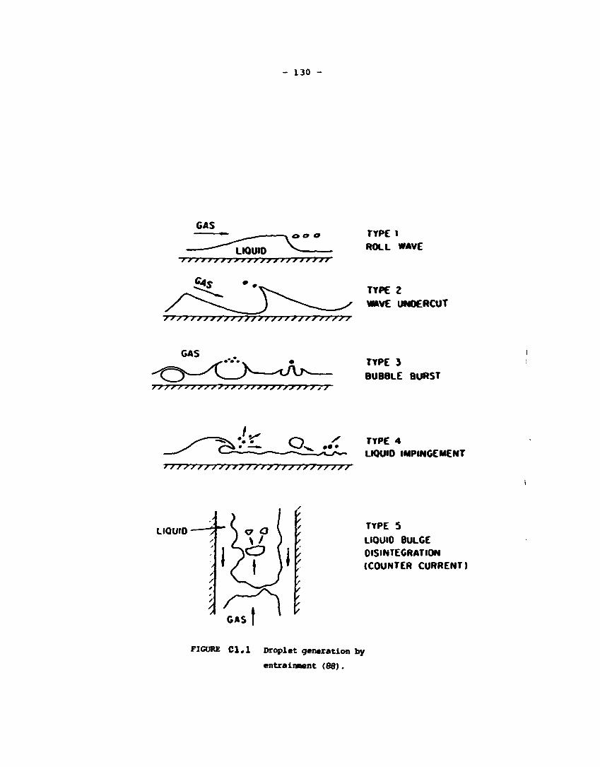
- 130 -
GAS TYP£ 1
ROLL WAVE
TYPE 2
WAVE UN0ERCUT
////////r/7/7777777/777/7/7/
GAS
77/77 S 77/7777>77/7/7//>777;7
TYPE 5
BUBBLE BURST
f/777777777/7 7 7/777/777777/
LIQUIO TYPE 5 LIQUIO BULGE DISINTEGRATION (COUNTER CURRENT)
FIGURE Cl.l Droplet generation by
entrainaent (88).
- 131 -
In the fourth type the iaping«ent of liquid «ass or droplets
•ay produce new droplets.
In counter-current flow the last type aay occur as a result
of flooding. Large amplitude waves aay be separated fro« the
liquid fil« to for« a liquid bridge. This «ay disintegrate into
several droplets.
Nuaerous saall droplets are generated in convection with the
quenching of the surface during the emergency cooling of the
fuel rods. The quenching area is the region on the cladding
surface where initial continuous contact between cladding sur
face and liquid is established i.e. the transition boiling
region before the return to nucleate boiling.
In post-CHF regions and in vapour-continous flow further drop
let generation can occur only through further breakup of larger
droplets to saaller ones due to hydrodynaaic forces or iapin-
geaent of the droplets on a hot surface with high velocity
and no rewetting.
Droplets Size.
The upper size liait of the droplet is given by the critical
Weber nuaber:
Pq - d - (Uq - u t )2
Ha M _ «*c
A aaxiaua stable droplet size is given by a critical Weber
nuaber of 12 - 13 (89). A value of 6.5 aay be suggested to re
present an average droplet size (10).
Droplet break up by iapingaent on a hot surface with a subse
quently high velocity has been exaained experiaentally. The
droplets will break up into a nuaber of saaller droplets de
pending on the perpendicuar velocity of the droplet at the
tiae of iapingaent.
- 132 -
The process is correlated in tens of Weber number:
ft • u | * d
P 7
with following classification
Hep £ 30 no break up
30 < wep £ 80 break up into a few large fragments
Hep > 80 break up into smaller fragments.
It should be noted that most experiments have been carried
out with flat plates with surfaces significantly larger than
the incoming droplets.
Experiments show that droplet populations can be divided
into two separate groups: a population of small droplets with
diameters from 10 i* to 140 H with a maximum number at 50-60 r
(90), and a population of large droplets with diameter from
300 it to 2000 |i with a maximum number at about 800 p (90,91).
The size and also the number distribution in the axial direction
depends primarily on the evaporation, i.e. interfacial heat
transfer. Coagulation and further break up due to grid spacers
in the fuel element and other channel restriction may also
play a role.
The small droplets have a larger surface-to-volume ratio than
large droplets i.e. the lifetime history is shorter for
small droplets, than for the larger droplets. The energy
absorption rate from these small droplets is very high so
long as the small droplets continues to exist.
The initial distribution of the two droplet populations is
characterized by a large but rapidly diminishing number of
small droplets and evolves into one relatively stable popula
tion of large droplets which are slowly diminishing in size.
- 133 -
These results may serve to explain qualitatively the observed
heat transfer phenomena near the return to nucleate boiling,
the near-field-theories (17).
Droplet Size Distribution.
Various theories on the formation of droplets usually predict
a single uniform size, cf. e.g. the critical Weber number men
tioned above.
As it is noted above, droplets are generated in populations
of various sizes. The droplets in a population generated by
the same mechanism, may be expected to be clustered around a
characteristic mean in a distribution which reflects the ran
domness in the process of generation, in other words be
stochastic in nature.
Droplet size distribution can be represented by a plot of the
number of droplets versus the diameter of droplets. The func
tion representing the plot has various names in the litera
ture: in the density function, the distribution curve or
frequency function.
The plot function is a number distribution function of the
droplets f(x) of a given diameter x. The total number of
droplets is then
m m
n » / dn * / f(x)dx.
The arithmetic mean of the diameter is defined as
_ • • / xf(x)dx x* - / xf(x)dx// f(x)dx -=*
-• -• n
the geometric mean diameter as
+• -lnxg * / lnxf(x)dx/ S f(x)dx.
- 134 -
The denominator is still simply equal to the total number.
In general a mean can be defined as
xab = / xaf(x)dx/ / xbf(x)dx.
If a is 3 and b 2 the mean most commonly used among the many
averages is the Sauter mean diameter.
When using a statistical mean diameter to correlate data, it
should be noticed , that it is important to use one that is
relevant to the problem. The field of application of the
Sauter mean diameter is in mass transfer and kinetics. When
mass distribution is in question the mean diameter based on
volume may be relevant, i.e. a is 3 and b zero. With respect
to evaporation the diameter alone or the volume-to-diameter
ratio may be relevant i.e.either a = 1, b = 0, or a = 3,
b = 1 (92).
Experimental examinations of droplet distributions on pro
bability paper show that droplet populations can be considered
as a distributed logarithmic normal (log-normal distribution)
(91) i.e.
dn dn = x • f(x) •
d(lnx) dx
1 (lnx - lnxnq)2^
. , • exp [ - — — — ] , • 2n • Oq 2aq*
where xng is the number geometric mean diameter as defined
above and ag is the geometric standard deviation, ag » In a
If the distribution is based on the volume of the droplets i.e.
n V « / k • x3dn
o
- 135 -
then
dV dV = x • — * xf(x3) d(lnx) dx
1 , (lnx - lnx w a)2
vg' exP [ ^ 1'
and
/T? • ag ^ L 2o2
dV dn dn = kx3 • = kx4 • — = kx4 • f(x) d(lnx) d(lnx) dx
Using this on the number distribution gives:
dV k (lnx - lnx n q)2
e*P [ " ZZ 1 " d(lnx) / 2 n a_ F L 2o2
exp (3 lnx)
or
dV k (lnx - (lnxng + 3a 2)) 2
exp [ — 2 2 ] d(lnx) / 2 % a2 * L 2a2 ag g
exp (3 lnxng + ^ a\
A comparison of equation with the volume distribution shows that
lnxvg 5 lnXng + 3o2
if it can be shown that k • exp (31nvng + 9/2 ag2) - 1.0.
- 136 -
If the distribution is based on surface the result would be:
In xsg s lnxng + 2og2
and for the Sauter mean, the relation is
In xvsg 2 lnxng + 2.5og2.
Other number distribution functions have also been used. The
Nukiyama - Tanasawa distribution has the form (89):
f(x) - A • x^xpt-b • x").
A and b are normalization factors, whereas m and n are usually
integers which sometimes can be given physical significance.
This distribution function has been extensively used in
pneumatic atomization.
C2. Droplet flow
In the following some discussion will be given on forces acting
on droplets in the droplet-dispersed flow region. The discus
sion is by no means thought of as providing a thorough exa
mination of the topic but will rather furnish a general
overview of the phenomena with some deeper examinations of
specific details.
In analyzing the forces acting on the droplets and the rela
tive motion between the phases it is beneficial to start with
an examination of the momentum equations for the two phases.
In order to have a tractable set of equations these have to be
derived from the general local instantaneous form of the mo
mentum equations by applying some sort of averaging procedures,
usually the Eulerian space and time averaging. In this way the
microscopic local instant fluctuations of the fluid motion are
eliminated resulting in equations describing the collective
interactions of fluid particles. The averaging operations ap
plied to the basic equations are commutative meaning that the
order the averaging is carried out does not matter.
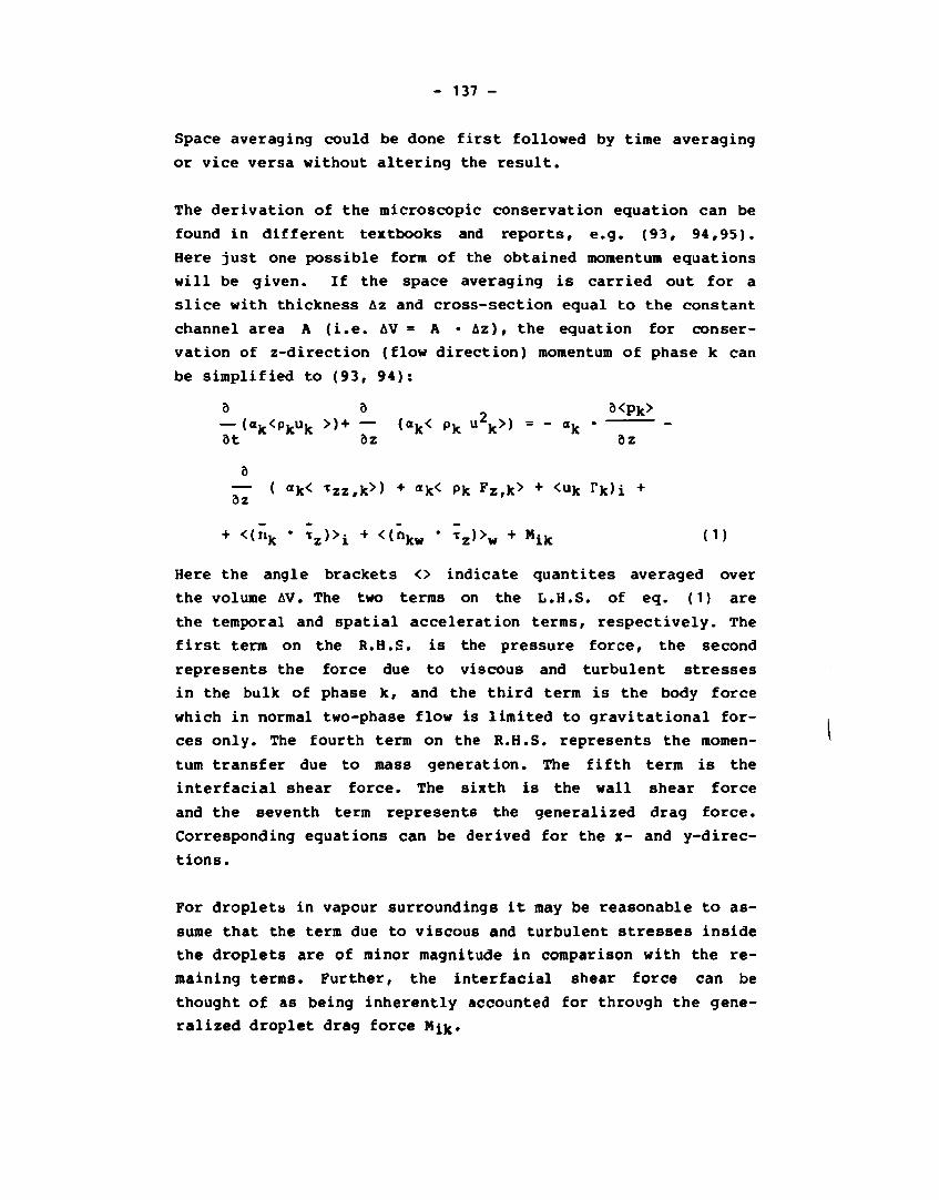
- 137 -
Space averaging could be done first followed by time averaging
or vice versa without altering the result.
The derivation of the microscopic conservation equation can be
found in different textbooks and reports, e.g. (93, 94,95).
Here just one possible form of the obtained momentum equations
will be given. If the space averaging is carried out for a
slice with thickness Az and cross-section equal to the constant
channel area A (i.e. AV = A • Az), the equation for conser
vation of z-direction (flow direction) momentum of phase k can
be simplified to (93, 94):
a a a<Pk> — <ak<pkuk » + — <ak< Pk u k>) - - a k * -at az az
a — ( ak< *zz,k>) + ak< Pk ?z,k> + <«k ?k)i + oz
+ <(nk • ;z)>i + <(nkw • ;2)>w + Mik (1)
Here the angle brackets <> indicate quantites averaged over
the volume AV. The two terms on the L.H.S. of eq. (1) are
the temporal and spatial acceleration terms, respectively. The
first term on the R.H.S. is the pressure force, the second
represents the force due to viscous and turbulent stresses
in the bulk of phase k, and the third term is the body force
which in normal two-phase flow is limited to gravitational for
ces only. The fourth term on the R.H.S. represents the momen
tum transfer due to mass generation. The fifth term is the
interfacial shear force. The sixth is the wall shear force
and the seventh term represents the generalized drag force.
Corresponding equations can be derived for the x- and y-direc-
tions.
For droplets in vapour surroundings it may be reasonable to as
sume that the term due to viscous and turbulent stresses inside
the droplets are of minor magnitude in comparison with the re
maining terms. Further, the interfacial shear force can be
thought of as being inherently accounted for through the gene
ralized droplet drag force H^.

- 138 -
Thus, the equation of motion in z-direction for the droplets
(liquid phase &) can be written as
-iftl-aXp, u, ] + d- £l-«>< plU2 ,>]- - (1- a) ̂ +
+ (1- <x)< Pl. Fz#1 >*<^l'Tl >i + «n1%f - 72>w *Hn <2>
where also the void fraction a has been introduced:
o = av
1- o = a, (3)
and the pressure has been assumed constant throughout the volume
AV.
The interfacial transfer terms in eq. (2) can be related through
the conservation equation across the interface, resulting in the
jump conditions, whence
< r x > + < rv> = o
MiX • *»iv " 0 (4)
As these terms appear as source terms in eq. (2) in its vapour
phase counterpart it is necessary to provide constitutive
equations for r^ and Hn . The equation for Mj.i will be
elucidated later on.
Equation (2) is given in the instantaneous volume average form
or area average form if the thickness Az of the slice is
taken sufficiently small. The different terms can now be time
averaged due to the commutative property of the averaging
operators. In that operation the form of the equation remains
exactly the same. Terms like
d_ a [d -a )< pxuji >)] become 7 [(1-o)< P I U A > ]
ot ot

- 139 -
where the overbar denotes time or statistical averaging. In
order to make eq (2) tractable it is necessary to separate
an average of a product into a product of averages. This can
be obtained by defining distribution coefficients of the form
(1-a)<u2,> c = :
(T^j • <ui>z (5)
The distribution coefficients depend on the flow and void frac
tion profiles. To illustrate the magnitude of the distribution
effects the coefficient C has been calculated for the power law
velocity and void fraction profiles shown in figure 1 (from ref.
(94)). For af flat velocity profile (m -»•») the distribution
coefficient equals unity and it deviates significantly from
unity only for very peaked velocity profiles. Thus, for high
velocity droplet flow where the velocity profile usually is
flat it seems reasonable to assume C=1.0. For lower velocities
the distribution effect becomes increasingly important and
then it is also necessary to incorporate the droplet concen
tration evaluated at the wall which has been shown to have
pronounced influence on the distribution coefficient (96).
It is felt that this wall concentration of droplets can be
closely related to the liquid film breakdown at the locus
of dryout and thus be one parameter when explaining the near
and far field post-CHF heat transfer regions found in experi
ments.
Another approach for dealing with the distribution effects is
to set up conservation equations for each part of a phase in
which the distribution can be assumed fairly uniform (distri
bution coefficient set equal to unity). A study of the CHF
phenomena using this approach can be found in (97). Thus the
problem of treating the distribution coefficient is shifted
to one of regarding transfer relationships between the sepa
rated parts of the two phases. This seems to be a more appeal
ing approach especially for film-type flow regions like
annular flow and for regions with an extremly peaked concen
tration profile like the subcooled boiling region.
In what now follows there will be a discussion of the constitu-
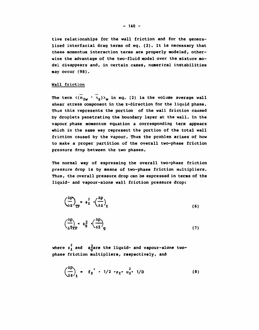
- 140 -
tive relationships for the wall friction and for the genera
lized interfacial drag terms of eq. (2). It is necessary that
these momentum interaction terms are properly modeled, other
wise the advantage of the two-fluid model over the mixture mo
del disappears and, in certain cases, numerical instabilities
may occur (98).
Wall friction
The term <(niw • tz)>w in eq. (2) is the volume average wall
shear stress component in the z-direction for the liquid phase.
Thus this represents the portion of the wall friction caused
by droplets penetrating the boundary layer at the wall. In the
vapour phase momentum equation a corresponding term appears
which in the same way represent the portion of the total wall
friction caused by the vapour. Thus the problem arises of how
to make a proper partition of the overall two-phase friction
pressure drop between the two phases.
The normal way of expressing the overall two-phase friction
pressure drop is by means of two-phase friction multipliers.
Thus, the overall pressure drop can be expressed in terms of the
liquid- and vapour-alone wall friction pressure drop:
VAZATO" l \LzK
,Ap,
'TP ~ ^bz'l (6)
VÅZTp 9 W'g (7)
2 o
where ^ and 4gare the liquid- and vapour-alone two-
phase friction multipliers, respectively, and
'AP> - ) - fx • 1/2 . p r Ujl. 1/D (8)
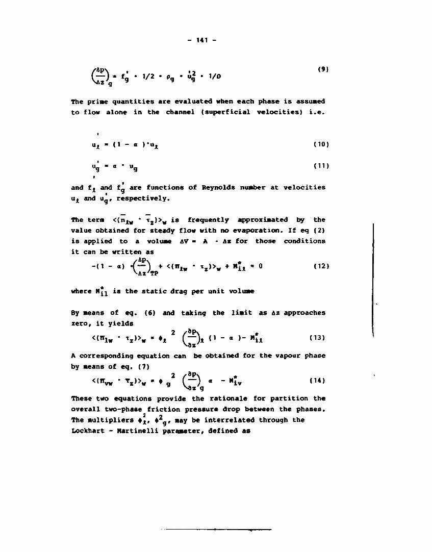
- 141 -
Og" £* " V2 ' "* ' ̂ ' V0 (9)
The prime quantities are evaluated when each phase is assumed
to flow alone in the channel (superficial velocities) i.e.
ux - (1 - a )*a1 (10)
Ug - « * Ug (ID
and f« and fa are functions of Reynolds nuaber at velocities
uA and ugf respectively.
The term <(nAw * *2)>w is frequently approximated by the
value obtained for steady flow with no evaporation. If eq (2)
is applied to a volume AV • A • A* for those conditions
it can be written as
-(1 - a) 4—\ • <(WJlw • xz)>w • HiA • 0 (12) ^Az'TP
where N ^ is the static drag per unit volume
By means of eq. (6) and taking the limit as Az approaches
zero, it yields
«ffiw * V>w * •! 2 (^)* n - « >- "u <13> A corresponding equation can be obtained for the vapour phase
by means of eq. (7) 2 /aP\ •
« n v w ' T z » w * » g Q ^ ) « ""iv <14>
These two equations provide the rationale for partition the
overall two-phase friction pressure drop between the phases. 2 o
The multipliers *x, •* , may be interrelated through the
Lockhart - Hartinelli parameter, defined as

- 142 -
4»2 X2 =-4 (15)
For turbulent flow with the single phase friction factor as
f= C0/Re0'2 this parameter can be expressed as
i — yp 1.8 _ ,. 0.2 x2 ( I _ » ) .(^;.(i^-) (16) " XE PA Hg
The Generalized Drag Force
The generalized drag force in eq. (2) is expressed as a total
force exchange per unit mixture volume. This can be related to
af total drag force FT per typical droplet by means of
1 - a Mi« = • FT (17)
11 Vd T
where V<j is the volume of a typical droplet.
The force PT can be divided into a number of forces some of
which can be shown to have a pronounced influence on the nume
rical stability of the two-fluid model. Here the following
forces will be dealt with: the skin and form drag force, vir
tual mass force, Basset force and forces due to asymmetrical
evaporation. Additional forces may be taken into account if
necessary for a specific analysis, e.g. diffusion forces due
to concentration gradients may be important in slow flow if
droplets are very nonuniformly distributed over the channel
cross sectional area. It is assumed that the total drag force
can be obtained simply by superposition of the included
forces.

- 143 -
The_ £>kin_and_Form £rag_For£e
This "standard" drag force acting on a droplet under steady
state conditions can be given as
Pjl*ur*|ur| FD = " CD — ' Ad <18>
where
CQ is a drag coefficient
A<3 is the projected area of the droplet facing the flow
uc is the relative velocity given by
ur = \ii - uv (19)
The total skin and drag force per mixture volume can be expres
sed as 1 - o pjur|ur|
PTD - ~ — * CD 1 * Ad <20>
For a dispersed flow system it is common to define some im
portant length scales (98, 99)
3 • Vd
Sauter mean radius r̂ ,, = (21) Ai
3 • Vd Drag radius VQ = (22)
rsm
^D
r e
*s
Ai
3 * Vd
4 • Ad
JL .
< &
\V3
1/2
Equivalent radius re =( * V^j (23)
/Ai\ V 2 Surface radius r8 =1 J (24)
Here A£ is the surface area of a typical droplet. For spherical
droplets these defined radii are all equivalent.
By introducing the area concentration given by
l-o ai - • Ai
Vd (25)

- 144 -
eq. (20) can be written by means of eqs. (21) and (23) as
CD rsm Pi * urlurl FTD * " ai * T ' — T" (2«>
4 rn 2
Thus the total skin and drag force per Mixture volume is pro
portional to the interfacial area concentration and the drag
force for the droplets. The ratio of the Sauter mean radius to
the drag radius can be thought of as a shape factor for the
droplets. For spherical droplets this shape factor equals unity.
It is evident that in order to have an accurate evaluation of FTD» Proper knowledge of the interfacial area concentration as
well as the drag coefficient is essential. The problems con
cerning the area concentration are closely related to the drop
let number density and are discussed in chapter CI. Here only
a few comments on the drag coefficient will be given.
The Drag Coefficient
A thorough examination of the drag coefficient in different
flow regions can be found in ref. (100, 101).
For a liquid droplet dispersed system there are two regions that
have to be separated: the viscous region or und is tor ted droplet
regions and the distorded droplet region. In the former the
viscosity has a pronounced influence on the droplet motion,
i.e. the drag coefficient is strongly dependent on the Reynolds
number of the droplets. In the latter region Cp is essentially
independent of Reynolds number.
For the viscous region two similarity hypothesis were intro
duced (100). Pirst it was assumed that the drag coefficient
CQ can be given as a function of the droplet Reynolds number
CD - CD (Red) (27)
where the Reynolds number was defined in terms of the mixture
viscosity ^ as
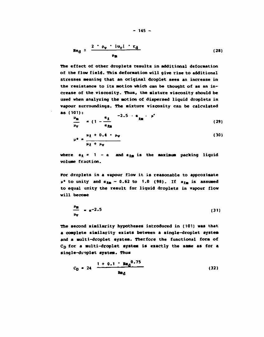
- 145 -
2 • pv * |url » rd
R«d = <28)
The effect of other droplets results in additional deformation
of the flow field. This deformation will give rise to additional
stresses meaning that an original droplet sees an increase in
the resistance to its motion which can be thought of as an in
crease of the viscosity. Thus, the mixture viscosity should be
used when analysing the motion of dispersed liquid droplets in
vapour surroundings. The mixture viscosity can be calculated
as (101): » « "2.5 - « - |»* *n *1 *m — - (1 - — (29) My «Jbl
uji + 0.4 • |iv (30) n* *
»*t • »*v
where *i * 1 - « and ajg is the maximum packing liquid
volume fraction.
For droplets in a vapour flow it is reasonable to approximate
p* to unity and a^ ~ 0.62 to 1.0 (98). If axu is assumed
to equal unity the result for liquid droplets in vapour flow
will become
— . «-2.5 (31) »»v
The second similarity hypotheses introduced in (101) was that
a complete similarity exists between a single-droplet system
and a multi-droplet system. Therfore the functional form of
C Q for a multi-droplet system is exactly the same as for a
single-droplet system. Thus
1 + 0 . 1 • H e d0 , 7 5
CD - 24 " (32) Re,j
- 146 -
This correlation indicates that Cn increases with a decreasing
vapour void fraction. For very small Reynolds nuaber (Re<) < 1)
eq. (32) reduces to the well-known Stokes drag law
In the distorted droplet region the single-droplet drag coeffi
cient depends only oa droplet radius and fluid properties (101)
4 /T~' T * rd * / _ T
'Ap Co- * 3 * *d * S—g (34)
It was assuaed (101) that for a aulti-droplet systea the increased drag due to other droplets was caused by the turbulent eddies in the droplets wake region in a siailar way as for a solid-particle systea and a aultiparticle systea, an equation for the drag coefficient of the aultiparticle systea was obtained in (101). Thus this equation coabined with eq. (34) was assuaed to be valid also for a aulti-droplet systea. By aeans of the approxiaation given by eq. (31) the following was obtained for a aulti-droplet systea (101):
1 + 17.67
18.67*
•
a
a
3
2. i j 4 /g • Ap CD - — rd / • 5 1 (35) D 3 a a 18.67* a *
This correlation indicates that the aoaentua coupling between
the phases increases with increasing droplet concentration
(decreasing void fraction a ).
Por a single droplet in an infinite aediua the viscous region
extends up to about Re. * 10 where
2r<j»Pvlur-l Re . = (36)
vv
ur« * u* ~ "v- <37>
u v - is the undisturbed vapour velocity. Por higher Reynolds nuaber the drag coefficient is essentially constant, i.e. the distorted droplet region is prevailing. In this region the
- 147 -
drag coefficient is proportional to the droplet size. Thus,
the upper limit of the drag coefficient is governed by the
maximum size of the droplet. This droplet size can be deter
mined from a critical Weber number:
2 p -u2.rd We = = 1 "
o The terminal velocity corresponding to eq (34) is
q«o«Ap V 4 u r. = /2-[ _ ^ ]
Pv
Eqs. (38) and (39) thus yield
rd*ax * 3 •/ g-Ap
which with eq. (34) gives the maximum drag coefficient CD=4.
There is no thorough treatise in ref. (101) of how to handle the
region transition for a multi-droplet system. A suggestion is to
assume that the transition occurs at Re ~ 10, where the Reynolds
number is based on the mixture viscosity according to eq.(28).
The above model was compared with one described by a large
number of experimental data where satisfactory agreements were
obtained for wide ranges of droplet concentration and Reynolds
number (98, 101). Thus, the similarity hypothesis discussed
above were concluded to be reasonable approach when developing
the multidroplet drag coefficient.
Virtual Mass Porce and Basset Force
The virtual mass force and the Basset force are transient
forces occurring when a particle (bubble, droplet) is accele
rating relative to the surrounding phase (liquid, vapour).
When a droplet is moving in vapour surroundings these forces
are usually very small compared, for instance, to the drag
force. Bowever, despite of its magnitude it has been shown
(38)
(39)
(40)

- 148 -
that the virtual mass force in particular has a pronounced
influence on the numerical stability of the two-fluid model
(102).
The virtual mass force can be explained briefly as follows:
when a particle is set in motion relative to the surrounding
medium it is given kinetic energy. In addition, the fluid
which it displaces by its movement also is given a certain
amount of kinetic energy. The total work done in accelerating
the particle is therefore greater than if only the particle
itself were moved, and the result is the same as if the mass
of the particle were increased by a specified amount. This
extra amount of mass is known as the added mass or induced
mass of the particle, and the sum of the actual mass and the
added mass is known as the virtual mass. It can be shown by
potential flow theory (103) that for a sphere in unrestricted
three-dimensional flow the added mass is half the mass of the
fluid displaced by the sphere.
The forms of the virtual mass force and the Basset force for a
collection of droplets simultaneously accelerating in the vapour
phase are not firmly established. Newer and more adequate
formulations of these forces are continually reported.
Zuber (104) studied the effect of concentration on the virtual
mass force. From potential theory outlined in (105) and assuming
low droplet concentration Zuber obtained an expression for the
virtual mass force acting on one representative droplet as
3-2<x dur
Fv s -Pv'V* (41)
a dt
where as before a is the vapour void fraction and ur the relative
velocity as in eq. (19). Py'V^ is the added or induced
mass for one droplet. For a spherical droplet Vj* can be
expressed as
1 * V l * '• 7 (2 • rsm> <42>
2 6

- 149 -
Equation (41) is valid for accelerating a spherical droplet
in the centre of a vapour-filled hollow fixed sphere. The
radius of the hollow sphere is taken so that at this distance
from the droplet the vapour is assumed to be undisturbed.
In ref. (106) a reinterprecation of Zuber's result is made
where the induced vapour flow caused by the droplet motion was
also taken into account. From this analysis the virtual mass
force became
dur Fv = -pv-V1*-a (43)
dt
In ref. (101) a new form of Fy is proposed based on Zuber's
result and the work reported in (102). The resulting equation is
3-2<x 3ur duv Fv = -pv'VJl* '( -ur ) (44)
a dt dz
Equations (43) and (44) reveal quite a different trend when
the void fraction decreases (droplet concentration increases).
For decreasing void fraction the virtual mass force decreases
accordingly to eq. (43) while it increases following eq. (44).
which one is most accurate is not readily pointed out. They
represent both small terras compared to other forces and contri
bute only by a minor amount to the numerical result while their
influence en the numerical stability is quite definite. In
view of both their small magnitude for droplet dispersed flow
and the overall uncertainty concerning the droplet shape and
size distributions in full-scale systems it is not worthwhile
to examine this issue more deeply here. Thus, the different
formulations, eqs. (43) and (44), can be taken as evidence on
the uncertainty in the present state of the art and it is
expected that further research will shed more light on these
phenomena.
The Basset force is the result of acceleration on the viscous
drag and boundary layer development around the droplets. This

- 150 -
force can be expressed as (c.f. ref. (104))
dur d£ F = -6-r2 /* p„*nm / (45) B ~ " L '" ^v ^m t at, /FT
where r is the droplet radius and \tm the mixture viscosity
according to eqs. (29) and (30). The integration is carried out
for the acceleration time span.
In ref. (104) an analysis is carried out to find out under what
conditions the Basset force can be neglected in comparison with
the virtual mass force. By means of the mean value theorem of
integral calculus the integral of eq. (45) can be related to
the time function:
t dur d£ dur
/ r £ 2 • • /£ (46) o dC /"E^t dt
By comparing the Basset force using eq. (46) with the virtual
mass force, eq. (44), assuming that the spatial derivative is
zero the following is obtained:
1 PV*VA* a 2
t< * ^ ( ) <47>
216 w r'nm 3-2a
As long as the acceleration time t obeys eq. (47) the Basset
force can be neglected. Normally for fast transients in droplet-
dispersed flow eq. (47) is fulfilled and thus the Basset force
is of minor importance.
Evaporation Forces
The evaporation forces have transverse directions resulting in
droplet movements in a plane normal to the flow direction away
from the heat transfer surface. Because of the high temperature
gradient inside the thermal boundary layer at the heat transfer
surface a droplet residing within this layer will experience a
nonuniform evaporation. The droplet side facing the heat transfer
surface will have a higher vapour generation than the opposite
- 151 -
droplet side resulting in different vapour velocities normal to
the droplet surface. This will create a force with a tendency
to push the droplet away from the heat transfer surface. It
can be expected that these evaporation forces give rise to
substantial droplet transversal trajectories at the locus of CHF
when the wall liquid film is boiled off and thus can be one
major aspect to be taken into account when modelling the near-
and far-field post-CFH heat transfer regions observed in expe
riments (17).
The derivation is quite straightforward. In (107) a linear
temperature gradient within the thermal boundary is assumed:
T = T S A T + (TW-TSAT)'(1- _) (48)
and by assuming a constant heat transfer coefficient between
the droplet surface and superheated vapour an integration of
vapour generation for each half of the droplet yields the fol
lowing average vapour velocities normal to the wall surface
h y d <Tw-TSAT>[0-7> + 7
Hf„'P„ * 46
uh = * (TW-TSAT)[(1- ~) + — 1 (49) "Ifg'Pv
u c = — — ' (TW-TSAT)[(1- h +-- ] (50) Hfg*Pv 6 46
for the hot and cold side of the droplet, respectively.
These velocities give rise to a resulting accelerating force
according to
pE ' Pv * V («h-uc> <51> 4
By means of eqs. (49) and (50) the force i s obtained as
nd2 h2 „ d ?R " T * T~2 (Tw-TSAT>
4 H-^ 'p . ,
2. Z^. y PE - ; ( T „ - T S M , r - — ' ( 1 - ~ ) (52)
fg -Pv 6 6
This force is expressed for one droplet and is of course active only within the boundary layer.
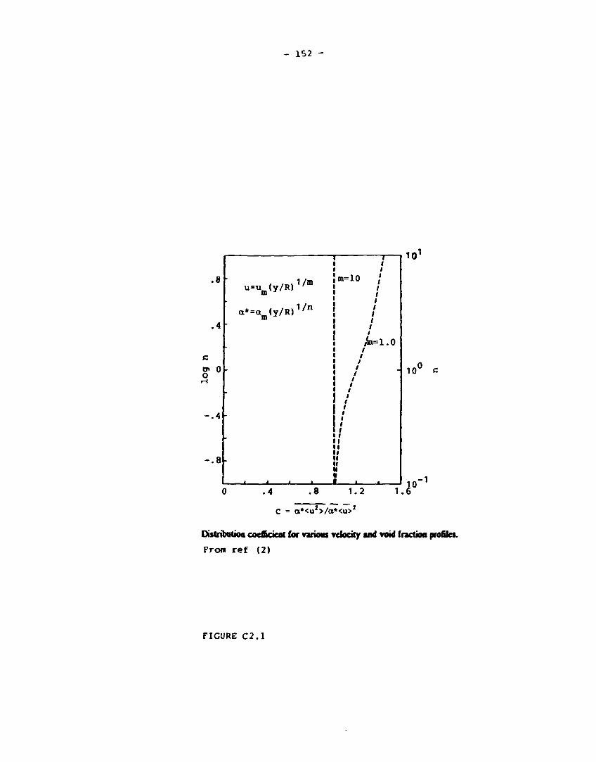
- 152 -
u=uffl(y/R)
a*=am(y/R)
1/m
1/n
m=10
f * i i i
,{a=1.0
I
8 1.2
c = a*<u2>/a*<u>2
101
10
1 . 6 ° -1
Distribotion coeflicieitt (or various velocity and void (ractioa profiles.
From r e f (2)
FIGURE C2 .1
- 153 -
C3. Droplet flow heat transfer.
The problems of heat transfer will be considered here in general.
Some correlations are proposed, but no evaluations with a com
puter programme including these correlations have been performed.
In order to find the best fit correlation comparisons with
experiments are needed using a computer programme including
different proposed correlations. The correlations discussed
are representative in such a way that they have been used in
several two-fluid programmes or in simple mechanistical program
mes for the modelling of droplet-dispersed flow heat transfer.
The examination of the modelling of heat transfer must start
with the energy equation for two-phase flow. The equations are
derived as local, instantaneous differential equations for
three-dimensional flow. The equations are written in an
Eulerian form, where the diffusion term is neglected. The real
physics cannot be calculated using microscopic volumes in a
class of few millimeters, which is the scale of basic subpro-
cesses in two-phase flow. For microscopic volume used in
calculating different kinds of averaging procedures must be
used, including both averaging in space and time. In this
chapter two averaging procedures for space will be defined.
The volume averaging denoted with angle brackets (<>) means
instantaneous averaged conditions in the volume. The time
average denoted with an overbar (~) means the statistical
average value for the volume average, e.g. that resulting from
many repeated measurements with same experimental conditions.
The time averaging is possible before volume averaging, too.
The local temperature measurement with a single thermocouple
is an example of this.
The thermocouple may give a good average for the local tem
perature, but the value may not be representative as a volume
average. The generalized conservation equations for two-phase
flow system may be written as (93)
- 154 -
_Ya k<p k¥ k>y — K < n z • (pk Tkvk+jk)^+ak<pkSk> 5t\ ' bz ^ S
1 - 1 -- - - / (ik »k+jk • nk)dS - - / n k w • jkdS
V ai v ajw
The pk ¥k is a generalized phase quantity to be considered,
ak the phase volume fraction defined as a instantaneous volu
metric fraction for the phase {= <<xk>), nz the direction ved-
tor in the axial direction, n k the direction vector perpendicular
to the interphase surface, j k the flux of ?k, and Sk the source of
The interfacial mass transfer rate may be written as
™k " Pk"k ' (vk - Vi)
The generalized form may be used for the derivation of the
conservation equations for each quantity, as mass, momentum
in the z direction, and energy. The quantities ?k, j k and Sk
have separate meanings for the mass conservation equation, momen
tum conservation equation, and energy conservation equation.
Here only the energy conservation equation will be considered.
For the energy equation the generalized terms are:
*k " Ek - <ek + 4/2)
h ' k̂ + (Pk1 - "k> • ^k
sk " *"k ' vjc + Qk
Here e k is internal energy (e = h - P/p)r qk beat flux to
phase k, pk pressure of phase k, I identity tensor, tk stress
tensor, Qk heat source in the fluid, Pk external force like
gravity potential in the fluid, vk velocity field in the fluid,
and uk the velocity component in the z-direction.
- 155 -
In addition to the voluae averaging, voluse-averaged quantities
have been defined in the equation over both the interfacial
and wall contact areas. These integrals are included into the
generalized equation. The voluae averaging discussed earlier
is defined by an integral
< > = 1/V / ( )
Further, the interfacial juap conditions are needed for two
phase flow. The generalized juap conditions may be expressed
as:
E (Pk*k(vjc - vi) • jk) • nk = 0 k=1
The averaging procedure is needed as well for interfacial jump
conditions as for the original conservation equations. A dis
cussion is needed for further understanding of two-phase physics
of what is vanishing froa physical reality due to other simpli
fications during the averaging process.
The real two-phase flow includes a high degree of turbulence.
Both voluae- and tiae-averaging do not take this subprocess
into account. This process aay be significant for the mixing
and is the origin for the crosswise movement of droplets causing
the iapingaent on the wall and enchances the wall heat transfer.
The voluae average describes only one velocity component for
each phase in each coordinate direction and then the informa
tion on real velocities for different droplet sizes vanishes.
If this inforaation should be conserved, the conservation
equations for a single liquid have to be split into equations
for two droplet classes. The aethod based on distribution func
tions will be discussed later. If different field equations for
one phase have been derived, a question may arise as to which
interfacial juap conditions are valid between different droplet
classes and between droplet. The impingment may be expected

- 156 -
to cause mass transfer and momentum transfer terms between
fractions, but modelling problems for energy equation may be
overstated due to small enthalpy differences.
In further simplifications the phase pressures are assumed to
be the same, i.e. p - p-j = P2« Then in the interfacial jump
condition, the differential terms for the phase pressures <Pli> ~ <P2i> vanishes. This pressure difference between phases
is significant in the energy equation during rapid blowdown
conditions, when the initiation of flashing is delayed. The
pressure inside microscopic vapour bubbles is higher than in
the water, corresponding to the difference in saturation tem
perature of 3....10 K. If different phase pressure are not
calculated, the delay has to be included into interfacial heat
transfer correlations.
The water pressure inside droplets is slightly higher than in
the vapour pressure around them, depending on the surface
tension and droplet diameter. This is the reason, why a cloud
of very small droplets may exist in superheated vapour for
quite a long time without evaporation. The mass of these micro-
size droplets is small, however, and they are not needed to be
considered separately in the energy conservation equation.
After assuming same phase pressures the only pressure terms
in the energy equation are
a . N a<xk _ («k<pku^ and <Pk> _ _
The kinetic energy conservation equation is usually used toge
ther with the momentum conservation equation for modelling
pressure losses of the real structure. The pressure losses in
Venturis and area changes may be changed to reversible and
irreversible pressure losses.

- 157 -
The generalized conservation equation cannot be used for com
parison with experimentally measured parameters, because usual
instruments measure only local parameters which may be time
averaged e.g. a gamma beam void fraction measurement where the
single beam signals may be considered as time averaged and the
volume average has to be calculated as a combination of parallel
time averages.
The time average for main parameters, velocity and enthalpy,
are defined as
«k<uic> <uk> =
*k
Because the main parameter can be directly chosen as time
average in conservation equations, no further interpretation
is needed between primitive and averaged parameters in equations.
The problem is how to formulate time averages for terms con
sisting of products of several main parameters. It is well known
from the combination rule, that the average of a product is not
equal to the product of two averages. Theorists have proposed
a solution to overcome the combination rule by the use of
distribution parameters that take into account the different
conditions over the cross section.
The distribution parameters may be used both in momentum and
energy conservation equations. There is a disadvantage, however,
that distribution parameters defined for different subprocesses
differ unless the processes are analogous. The convective term
in the differential equation needs the averaging of <ax><hjcujc>.
- 158 -
The distribution parameter for the energy equation requires
e.g. the distribution parameter
ck " «k<nkuk>
«k<hkxuk>
The corresponding distribution parameters are needed for the
interfacial jump condition, as for the interfacial surface
area. In practice very few data distribution parameters exists
and the parameter in computer models is usually set to unity.
The situation typically reflects disagreements between theorists
and programme developers. Although a theorist recommends the
use of distribution parameters for the complicated two-phase
flow form including droplet and film fields, the programme
developer may find it easier to use split field equations.
The use of distribution parameters is easier for a droplet field
that consists of several droplet sizes. Then the log-normal
distribution can be used as a basis in the calculation of
distribution parameters.
The distribution parameter becomes significant for vapour en
thalpy convection if a nonflat vapour temperature profile
must be expected over the cross section. This is possible, e.g.
in a rod bundle, where the periphery of the bundle is not so
hot as the central part.
Por the discussion of problems in modelling of interfacial
heat transfer the interfacial area is very essential, because
the heat flux is expressed as a product of heat transfer coef
ficient, interfacial surface area and temperature difference
between superheated vapour and interfase. The interfacial area
is related to void fraction and droplet diameter by:
2 6 (• - a) Aj « n * d »
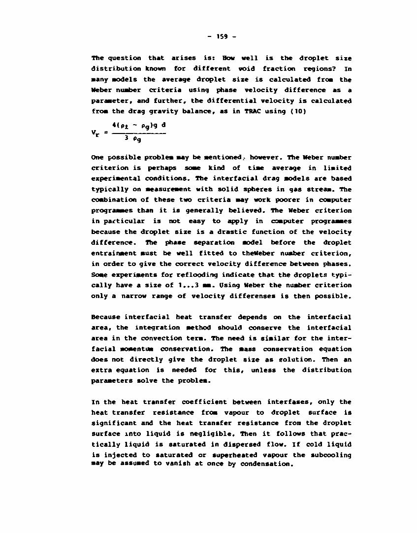
- 159 -
The question that arises is: How well is the droplet size
distribution known for different void fraction regions? In
•any models the average droplet size is calculated froa the
Weber nuaber criteria using phase velocity difference as a
parameter, and further, the differential velocity is calculated
froa the drag gravity balance, as in TRAC using (10)
+ (P1 - Pg)g <* V_ =
3 Pg
One possible problea aay be mentioned- however. The Weber nuaber
criterion is perhaps soae kind of tiae average in liaited
experimental conditions. The interfacial drag aodels are based
typically on aeasureaent with solid spheres in gas streaa. The
combination of these two criteria aay work poorer in computer
prograaaes than it is generally believed. The Weber criterion
in particular is not easy to apply in computer prograaaes
because the droplet size is a drastic function of the velocity
difference. The phase separation aodel before the droplet
entrainaent aust be well fitted to theWeber nuaber criterion,
in order to give the correct velocity difference between phases.
Soae experiaents for reflooding indicate that the droplets typi
cally have a size of 1...3 aa. Using Weber the nuaber criterion
only a narrow range of velocity differenses is then possible.
Because interfacial heat transfer depends on the interfacial
area, the integration aethod should conserve the interfacial
area in the convection tera. The need is siailar for the inter
facial aoaentua conservation. The aass conservation equation
does not directly give the droplet size as solution. Then an
extra equation is needed for this, unless the distribution
parameters solve the problea.
In the heat transfer coefficient between interfases, only the
heat transfer resistance froa vapour to droplet surface is
significant and the heat transfer resistance from the droplet
surface into liquid is negligible. Then it follows that prac
tically liquid is saturated in dispersed flow. If cold liquid
is injected to saturated or superheated vapour the subcooling aay be assumed to vanish at once by condensation.
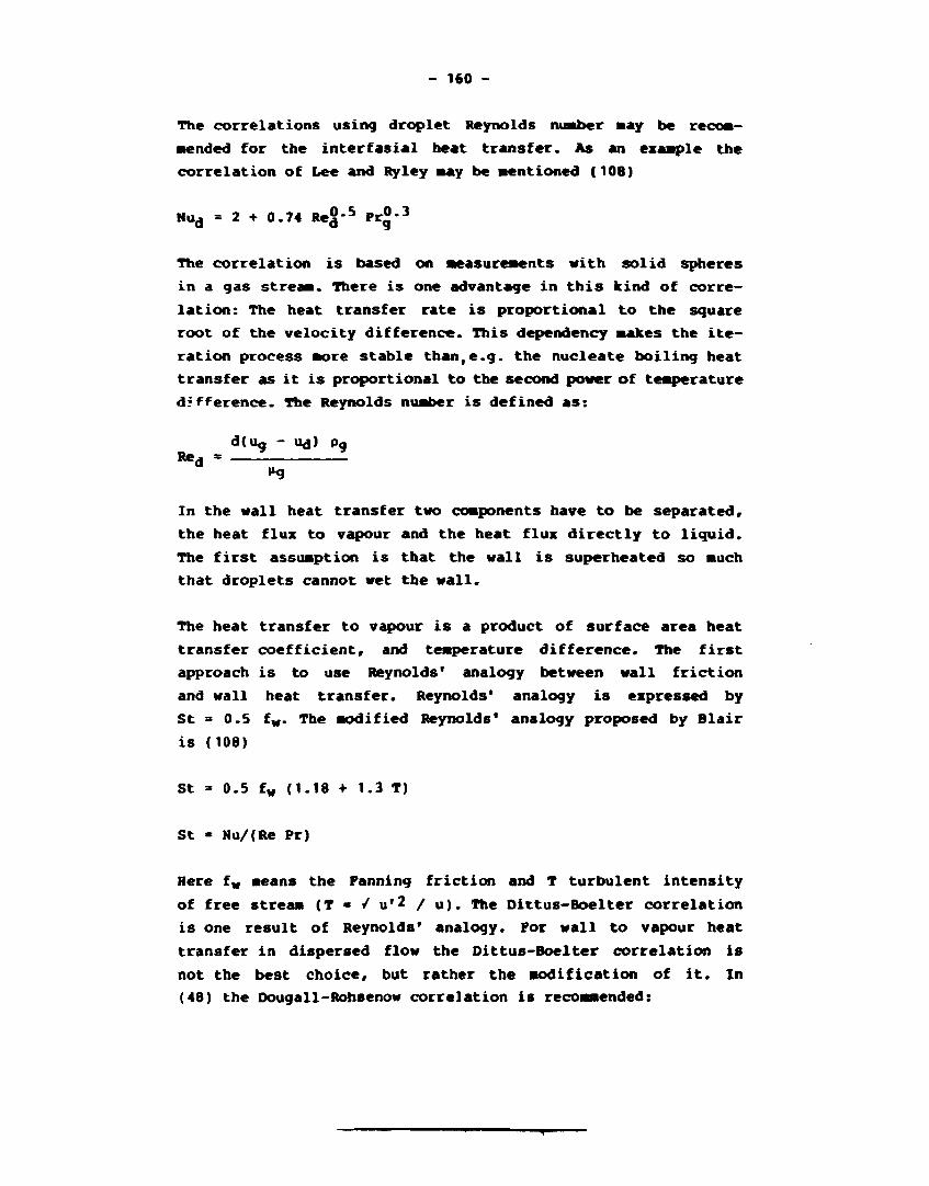
- 160 -
The correlations using droplet Reynolds number aay be recoa-
aended for the interfasial heat transfer. As an exaaple the
correlation of Lee and Ryley aay be mentioned (108)
Hud - 2 + 0.74 Re£'5 Pr°-3
The correlation is based on aeasureaents with solid spheres
in a gas streaa. There is one advantage in this kind of corre
lation: The heat transfer rate is proportional to the square
root of the velocity difference. This dependency makes the ite
ration process aore stable than,e.g. the nucleate boiling heat
transfer as it is proportional to the second power of teaperature
difference. The Reynolds nuaber is defined as:
d(Ug - 114) pg
In the wall heat transfer two coaponents have to be separated,
the heat flux to vapour and the heat flux directly to liquid.
The first assumption is that the wall is superheated so auch
that droplets cannot wet the wall.
The heat transfer to vapour is a product of surface area heat
transfer coefficient, and teaperature difference. The first
approach is to use Reynolds' analogy between wall friction
and wall heat transfer. Reynolds' analogy is expressed by
St • 0.5 fw. The modified Reynolds' analogy proposed by Blair
is (108)
St = 0.5 fw (1.18 + 1.3 T)
St - Mu/(Re Pr)
Here fw means the Panning friction and T turbulent intensity
of free stream (T * / u'2 / u). The Dittus-Boelter correlation
is one result of Reynolds' analogy. For wall to vapour heat
transfer in dispersed flow the Dittus-Boelter correlation is
not the best choice, but rather the modification of it. In
(48) the Dougall-Rohsenow correlation is recommended:
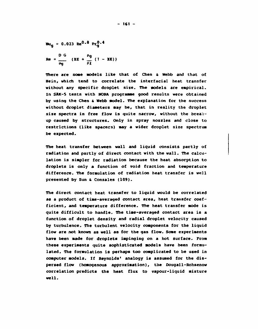
- 161 -
Hug • 0.023 Re0*8 PrJ*4
D G pq Re = (XE • (1 - » ) )
i<g PI
There are some models like that of Chen & Webb and that of
Hein, which tend to correlate the interfacial heat transfer
without any specific droplet size. The models are empirical.
In SAK-5 tests with NORA programme good results were obtained
by using the Chen & Webb model. The explanation for the success
without droplet diameters may be, that in reality the droplet
size spectra in free flow is quite narrow, without the break
up caused by structures. Only in spray nozzles and close to
restrictions (like spacers) may a wider droplet size spectrum
be expected.
The heat transfer between wall and liquid consists partly of
radiation and partly of direct contact with the wall. The calcu
lation is simpler for radiation because the heat absorption to
droplets is only a function of void fraction and temperature
difference. The formulation of radiation heat transfer is well
presented by Sun & Conzales (109).
The direct contact heat transfer to liquid would be correlated
as a product of time-averaged contact area, heat transfer coef
ficient, and temperature difference. The heat transfer mode is
quite difficult to handle. The time-averaged contact area is a
function of droplet density and radial droplet velocity caused
by turbulence. The turbulent velocity components for the liquid
flow are not known as well as for the gas flow. Some experiments
have been made for droplets impinging on a hot surface. Prom
these experiments quite sophisticated models have been formu
lated. The formulation is perhaps too complicated to be used in
computer models. If Reynolds' analogy is assumed for the dis
persed flow (homogenous approximation), the Dougall-Rohsenow
correlation predicts the heat flux to vapour-liquid mixture
well.

- 162 -
The direct liquid contact heat transfer has been applied in
many programmes. The model is very simple in the German re-
flooding programme FLUT. Varone (110) has used a complicated
model proposed by Kendall f Rohsenow in his own programme.

ISBN 87-550-1109-8
ISSN 0418-6435
mlnmb/goub Stockholm 1985
Top Related