arX

iv:g

r-qc

/040

5033

v1 6

May

200

4

GRAVITY, GAUGE THEORIES ANDGEOMETRIC ALGEBRA

Anthony Lasenby1, Chris Doran2 and Stephen Gull3

Astrophysics Group, Cavendish Laboratory, Madingley Road,Cambridge CB3 0HE, UK.

Abstract

A new gauge theory of gravity is presented. The theory is constructedin a flat background spacetime and employs gauge fields to ensure thatall relations between physical quantities are independent of the positionsand orientations of the matter fields. In this manner all properties ofthe background spacetime are removed from physics, and what remainsare a set of ‘intrinsic’ relations between physical fields. For a wide rangeof phenomena, including all present experimental tests, the theory repro-duces the predictions of general relativity. Differences do emerge, however,through the first-order nature of the equations and the global properties ofthe gauge fields, and through the relationship with quantum theory. Theproperties of the gravitational gauge fields are derived from both classi-cal and quantum viewpoints. Field equations are then derived from anaction principle, and consistency with the minimal coupling procedure se-lects an action that is unique up to the possible inclusion of a cosmologicalconstant. This in turn singles out a unique form of spin-torsion interac-tion. A new method for solving the field equations is outlined and appliedto the case of a time-dependent, spherically-symmetric perfect fluid. Agauge is found which reduces the physics to a set of essentially Newtonianequations. These equations are then applied to the study of cosmology,and to the formation and properties of black holes. Insistence on find-ing global solutions, together with the first-order nature of the equations,leads to a new understanding of the role played by time reversal. This al-ters the physical picture of the properties of a horizon around a black hole.The existence of global solutions enables one to discuss the properties offield lines inside the horizon due to a point charge held outside it. TheDirac equation is studied in a black hole background and provides a quickderivation of the Hawking temperature. Some applications to cosmologyare also discussed, and a study of the Dirac equation in a cosmologicalbackground reveals that the only models consistent with homogeneity arespatially flat. It is emphasised throughout that the description of gravityin terms of gauge fields, rather than spacetime geometry, leads to manysimple and powerful physical insights. The language of ‘geometric alge-bra’ best expresses the physical and mathematical content of the theoryand is employed throughout. Methods for translating the equations intoother languages (tensor and spinor calculus) are given in appendices.

1E-mail: a.n.lasenby@mrao.cam.ac.uk2E-mail: c.doran@mrao.cam.ac.uk3E-mail: steve@mrao.cam.ac.uk

This paper first appeared in Phil. Trans. R. Soc. Lond. A (1998) 356, 487–582.The present version has been updated with some corrections and improvementsin notation. Some extra citations have been added, but these are not intendedto be an exhaustive catalogue of work since the paper was completed in 1996.

April 2004

Contents

1 Introduction 5

2 An outline of geometric algebra 9

2.1 The spacetime algebra . . . . . . . . . . . . . . . . . . . . . . . . 122.2 Geometric calculus . . . . . . . . . . . . . . . . . . . . . . . . . . 132.3 Linear algebra . . . . . . . . . . . . . . . . . . . . . . . . . . . . . 15

3 Gauge principles for gravitation 16

3.1 The position-gauge field . . . . . . . . . . . . . . . . . . . . . . . 173.2 The rotation-gauge field . . . . . . . . . . . . . . . . . . . . . . . 193.3 Gauge fields for the Dirac action . . . . . . . . . . . . . . . . . . 223.4 The coupled Dirac equation . . . . . . . . . . . . . . . . . . . . . 243.5 Observables and covariant derivatives . . . . . . . . . . . . . . . 26

4 The field equations 29

4.1 The h-equation . . . . . . . . . . . . . . . . . . . . . . . . . . . . 304.2 The Ω-equation . . . . . . . . . . . . . . . . . . . . . . . . . . . . 314.3 Covariant forms of the field equations . . . . . . . . . . . . . . . 334.4 Point-particle trajectories . . . . . . . . . . . . . . . . . . . . . . 354.5 The equivalence principle and the Newtonian limit . . . . . . . . 36

5 Symmetries, invariants and conservation laws 38

5.1 The Weyl tensor . . . . . . . . . . . . . . . . . . . . . . . . . . . 395.2 Duality of the Weyl tensor . . . . . . . . . . . . . . . . . . . . . . 405.3 The Petrov classification . . . . . . . . . . . . . . . . . . . . . . . 415.4 The Bianchi identities . . . . . . . . . . . . . . . . . . . . . . . . 425.5 Symmetries and conservation laws . . . . . . . . . . . . . . . . . 44

6 Spherically-symmetric systems 47

6.1 The ‘intrinsic’ method . . . . . . . . . . . . . . . . . . . . . . . . 476.2 The intrinsic field equations . . . . . . . . . . . . . . . . . . . . . 486.3 Static matter distributions . . . . . . . . . . . . . . . . . . . . . . 556.4 Point source solutions — black holes . . . . . . . . . . . . . . . . 576.5 Collapsing dust . . . . . . . . . . . . . . . . . . . . . . . . . . . . 666.6 Cosmology . . . . . . . . . . . . . . . . . . . . . . . . . . . . . . 72

7 Electromagnetism in a gravitational background 79

7.1 Characteristic surfaces . . . . . . . . . . . . . . . . . . . . . . . . 827.2 Point charge in a black-hole background . . . . . . . . . . . . . . 837.3 Polarisation repulsion . . . . . . . . . . . . . . . . . . . . . . . . 867.4 Point charge in a k > 0 cosmology . . . . . . . . . . . . . . . . . 87

2

8 The Dirac equation in a gravitational background 89

8.1 Black hole background . . . . . . . . . . . . . . . . . . . . . . . . 898.2 The Hawking temperature . . . . . . . . . . . . . . . . . . . . . . 948.3 The Dirac equation in a cosmological background . . . . . . . . . 95

9 Implications for cosmology 96

9.1 Cosmological redshifts . . . . . . . . . . . . . . . . . . . . . . . . 979.2 k 6= 0 cosmologies . . . . . . . . . . . . . . . . . . . . . . . . . . . 989.3 Mass and energy in cosmological models . . . . . . . . . . . . . . 98

10 Conclusions 99

A The Dirac operator algebra 101

B Some results in multivector calculus 102

C The translation of tensor calculus 104

3

Part I — Foundations

4

1 Introduction

In modern theoretical physics particle interactions are described by gauge theo-ries. These theories are constructed by demanding that symmetries in the lawsof physics should be local, rather than global, in character. The clearest ex-positions of this principle are contained in quantum theory, where one initiallyconstructs a Lagrangian containing a global symmetry. In order to promote thisto a local symmetry, the derivatives appearing in the Lagrangian are modified sothat they are unchanged in form by local transformations. This is achieved bythe introduction of fields with certain transformation properties (‘gauge fields’),and these fields are then responsible for inter-particle forces. The manner inwhich the gauge fields couple to matter is determined by the ‘minimal coupling’procedure, in which partial (or directional) derivatives are replaced by covariantderivatives. This is the general framework that has been applied so successfullyin the construction of the standard model of particle physics, which accountsfor the strong, weak and electromagnetic forces.

But what of gravity: can general relativity be formulated as a gauge theory?This question has troubled physicists for many years [1, 2, 3]. The first workthat recovered features of general relativity from a gauging argument was due toKibble [2], who elaborated on an earlier, unsuccessful attempt by Utiyama [1].Kibble used the 10-component Poincare group of passive infinitesimal coordi-nate transformations (consisting of four translations and six rotations) as theglobal symmetry group. By gauging this group and constructing a suitableLagrangian density for the gauge fields, Kibble arrived at a set of gravitationalfield equations — though not the Einstein equations. In fact, Kibble arrivedat a slightly more general theory, known as a ‘spin-torsion’ theory. The neces-sary modifications to Einstein’s theory to include torsion were first suggestedby Cartan [4], who identified torsion as a possible physical field. The connec-tion between quantum spin and torsion was made later [2, 5, 6], once it hadbecome clear that the stress-energy tensor for a massive fermion field must beasymmetric [7, 8]. Spin-torsion theories are sometimes referred to as Einstein–Cartan–Kibble–Sciama theories. Kibble’s use of passive transformations wascriticised by Hehl et al. [9], who reproduced Kibble’s derivation from the stand-point of active transformations of the matter fields. Hehl et al. also arrived at aspin-torsion theory, and it is now generally accepted that torsion is an inevitablefeature of a gauge theory based on the Poincare group.

The work of Hehl et al. [9] raises a further issue. In their gauge theory deriva-tion Hehl et al. are clear that ‘coordinates and frames are regarded as fixed onceand for all, while the matter fields are replaced by fields that have been rotatedor translated’. It follows that the derivation can only affect the properties of thematter fields, and not the properties of spacetime itself. Yet, once the gaugefields have been introduced, the authors identify these fields as determining thecurvature and torsion of a Riemann–Cartan spacetime. This is possible only if itis assumed from the outset that one is working in a Riemann–Cartan spacetime,and not in flat Minkowski spacetime. But the idea that spacetime is curved isone of the cornerstone principles of general relativity. That this feature mustbe introduced a priori , and is not derivable from the gauge theory argument, ishighly undesirable — it shows that the principle of local gauge invariance mustbe supplemented with further assumptions before general relativity is recovered.The conclusions are clear: classical general relativity must be modified by the

5

introduction of a spin-torsion interaction if it is to be viewed as a gauge theory,and the gauge principle alone fails to provide a conceptual framework for generalrelativity as a theory of gravity.

In this paper we propose an alternative theory of gravity that is derived fromgauge principles alone. These gauge fields are functions of position in a singleMinkowski vector space. But here we immediately hit a profound difficulty.Parameterising points with vectors implies a notion of a Newtonian ‘absolutespace’ (or spacetime) and one of the aims of general relativity was to banishthis idea. So can we possibly retain the idea of representing points with vectorswithout introducing a notion of absolute space? The answer to this is yes— we must construct a theory in which points are parameterised by vectors,but the physical relations between fields are independent of where the fieldsare placed in this vector space. We must therefore be free to move the fieldsaround the vector space in an arbitrary manner, without in any way affecting thephysical predictions. In this way our abstract Minkowski vector space will playan entirely passive role in physics, and what will remain are a set of ‘intrinsic’relations between spacetime fields at the same point. Yet, once we have chosena particular parameterisation of points with vectors, we will be free to exploitthe vector space structure to the full, secure in the knowledge that any physicalprediction arrived at is ultimately independent of the parameterisation.

The theory we aim to construct is therefore one that is invariant under arbi-trary field displacements. It is here that we make contact with gauge theories,because the necessary modification to the directional derivatives requires theintroduction of a gauge field. But the field required is not of the type usuallyobtained when constructing gauge theories based on Lie-group symmetries. Thegauge field coupling is of an altogether different, though very natural, character.However, this does not alter the fact that the theory constructed here is a gaugetheory in the broader sense of being invariant under a group of transformations.The treatment presented here is very different from that of Kibble [2] and Hehlet al. [9]. These authors only considered infinitesimal translations, whereas weare able to treat arbitrary finite field displacements. This is essential to our aimof constructing a theory that is independent of the means by which the positionsof fields are parameterised by vectors.

Once we have introduced the required ‘position-gauge’ field, a further space-time symmetry remains. Spacetime fields are not simply scalars, but also consistof vectors and tensors. Suppose that two spacetime vector fields are equatedat some position. If both fields are then rotated at a point, the same intrinsicphysical relation is obtained. We therefore expect that all physical relationsshould be invariant under local rotations of the matter fields, as well as dis-placements. This is necessary if we are to achieve complete freedom from theproperties of the underlying vector space — we cannot think of the vectors rep-resenting physical quantities as having direction defined relative to some fixedvectors in Minkowski spacetime, but are only permitted to consider relationsbetween matter fields. Achieving invariance under local rotations introduces afurther gauge field, though now we are in the familiar territory of Yang–Millstype interactions (albeit employing a non-compact Lie group).

There are many ways in which the gauge theory presented here offers bothreal and potential advantages over traditional general relativity. As our theoryis a genuine gauge theory, the status of physical predictions is always unam-biguous — any physical prediction must be extracted from the theory in a

6

gauge-invariant manner. Furthermore, our approach is much closer to the con-ventional theories of particle physics, which should ease the path to a quantumtheory. One further point is that discarding all notions of a curved spacetimemakes the theory conceptually much simpler than general relativity. For exam-ple, there is no need to deal with topics such as differentiable manifolds, tangentspaces or fibre bundles [10].

The theory developed here is presented in the language of ‘geometric alge-bra’ [11, 12]. Any physical theory can be formulated in a number of differentmathematical languages, but physicists usually settle on a language which theyfeel represents the ‘optimal’ choice. For quantum field theory this has becomethe language of abstract operator commutation relations, and for general rela-tivity it is Riemannian geometry. For our gauge theory of gravity there seemslittle doubt that geometric algebra is the optimal language available in whichto formulate the theory. Indeed, it was partly the desire to apply this languageto gravitation theory that led to the development of the present theory. (Thisshould not be taken to imply that geometric algebra cannot be applied to stan-dard general relativity — it certainly can [11, 13, 14, 15]. It has also beenused to elaborate on Utiyama’s approach [14].) To us, the use of geometricalgebra is as central to the theory of gravity presented here as tensor calculusand Riemannian geometry were to Einstein’s development of general relativity.It is the language that most clearly exposes the structure of the theory. Theequations take their simplest form when expressed in geometric algebra, andall reference to coordinates and frames is removed, achieving a clean separationbetween physical effects and coordinate artefacts. Furthermore, the geometricalgebra development of the theory is entirely self-contained. All problems canbe treated without ever having to introduce concepts from other languages, suchas differential forms or the Newman–Penrose formalism.

We realise, however, that the use of an unfamiliar language may deter somereaders from exploring the main physical content of our theory — which is ofcourse independent of the language chosen to express it. We have thereforeendeavoured to keep the mathematical content of the main text to a minimumlevel, and have included appendices describing methods for translating our equa-tions into the more familiar languages of tensor and spinor calculus. In addition,many of the final equations required for applications are simple scalar equations.The role of geometric algebra is simply to provide the most efficient and trans-parent derivation of these equations. It is our hope that physicists will findgeometric algebra a simpler and more natural language than that of differentialgeometry and tensor calculus.

This paper starts with an introduction to geometric algebra and its space-time version – the spacetime algebra. We then turn to the gauging argumentsoutlined above and find mathematical expressions of the underlying principles.This leads to the introduction of two gauge fields. At this point the discussionis made concrete by turning to the Dirac action integral. The Dirac action isformulated in such a way that internal phase rotations and spacetime rotationstake equivalent forms. Gauge fields are then minimally coupled to the Diracfield to enforce invariance under local displacements and both spacetime andphase rotations. We then turn to the construction of a Lagrangian densityfor the gravitational gauge fields. This leads to a surprising conclusion. Thedemand that the gravitational action be consistent with the derivation of theminimally-coupled Dirac equation restricts us to a single action integral. The

7

only freedom that remains is the possible inclusion of a cosmological constant,which cannot be ruled out on theoretical grounds alone. The result of this workis a set of field equations that are completely independent of how we choose tolabel the positions of fields with a vector x. The resulting theory is conceptu-ally simple and easier to calculate with than the metric-based theory of generalrelativity. We call this theory ‘gauge theory gravity’ (GTG). Having derivedthe field equations, we turn to a discussion of measurements, the equivalenceprinciple and the Newtonian limit in GTG. We end Part I with a discussion ofsymmetries, invariants and conservation laws.

In Part II we turn to applications, concentrating mainly on time-dependentspherically-symmetric systems. We start by studying perfect fluids and derivea simple set of first-order equations that describe a wide range of physical phe-nomena. The method of derivation of these equations is new and offers manyadvantages over conventional techniques. The equations are then studied inthe contexts of black holes, collapsing matter and cosmology. We show howa gauge can be chosen that affords a clear, global picture of the properties ofthese systems. Indeed, in many cases one can apply simple, almost Newtonian,reasoning to understand the physics. For some of these applications the pre-dictions of GTG and general relativity are identical, and these cases includeall present experimental tests of general relativity. However, on matters suchas the role of horizons and topology, the two theories differ. For example, weshow that the black-hole solutions admitted in GTG fall into two distinct time-asymmetric gauge sectors, and that one of these is picked out uniquely by theformation process. This is quite different to general relativity, which admits eter-nal time-reverse symmetric solutions. In discussing differences between GTGand general relativity, it is not always clear what the correct general relativisticviewpoint is. We should therefore be explicit in stating that what we intendwhen we talk about general relativity is the full, modern formulation of thesubject as expounded by, for example, Hawking & Ellis [16] and D’Inverno [17].This includes ideas such as worm-holes, exotic topologies and distinct ‘universes’connected by black holes [18, 19].

After studying some solutions for the gravitational fields we turn to theproperties of electromagnetic and Dirac fields in gravitational backgrounds. Forexample, we give field configurations for a charge held at rest outside a blackhole. We show how these field lines extend smoothly across the horizon, andthat the origin behaves as a polarisation charge. This solution demonstrateshow the global properties of the gravitational fields are relevant to physics out-side the horizon, a fact that is supported by an analysis of the Dirac equation ina black-hole background. This analysis also provides a quick, though physicallyquestionable, derivation of a particle production rate described by a Fermi–Diracdistribution with the correct Hawking temperature. We end with a discussion ofthe implications of gauge-theory gravity for cosmology. A study of the Maxwelland Dirac equations in a cosmological background reveals a number of surpris-ing features. In particular, it is shown that a non-spatially-flat universe does notappear homogeneous to Dirac fields — fermionic matter would be able to detectthe ‘centre’ of the universe if k 6= 0. Thus the only homogeneous cosmologicalmodels consistent with GTG are those that are spatially flat. (This does notrule out spatially-flat universes with a non-zero cosmological constant.) A con-cluding section summarises the philosophy behind our approach, and outlinessome future areas of research.

8

2 An outline of geometric algebra

There are many reasons for preferring geometric algebra to other languages em-ployed in mathematical physics. It is the most powerful and efficient languagefor handling rotations and boosts; it generalises the role of complex numbersin two dimensions, and quaternions in three dimensions, to a scheme that effi-ciently handles rotations in arbitrary dimensions. It also exploits the advantagesof labelling points with vectors more fully than either tensor calculus or differ-ential forms, both of which were designed with a view to applications in theintrinsic geometry of curved spaces. In addition, geometric algebra affords anentirely real formulation of the Dirac equation [20, 21], eliminating the needfor complex numbers. The advantage of the real formulation is that internalphase rotations and spacetime rotations are handled in an identical manner ina single unifying framework. A wide class of physical theories have now beensuccessfully formulated in terms of geometric algebra. These include classicalmechanics [22, 23, 24], relativistic dynamics [25], Dirac theory [20, 21, 26, 27],electromagnetism and electrodynamics [12, 26, 28], as well as a number of otherareas of modern mathematical physics [29, 30, 31, 32, 33]. In every case, geomet-ric algebra has offered demonstrable advantages over other techniques and hasprovided novel insights and unifications between disparate branches of physicsand mathematics.

This section is intended to give only a brief introduction to the ideas andapplications of geometric algebra. A fuller introduction, including a number ofresults relevant to this paper, is set out in the series of papers [12, 21, 26, 31]written by the present authors. Elsewhere, the books by Doran & Lasenby [34],Hestenes [14, 22] and Hestenes & Sobczyk [11] cover the subject in detail. Anumber of other helpful introductory articles can be found, including those byHestenes [35, 36], Vold [24, 28], and Doran & Lasenby [37]. The conferenceproceedings [38, 39, 40] also contain some interesting and useful papers.

Geometric algebra arose from Clifford’s attempts to generalise Hamilton’squaternion algebra into a language for vectors in arbitrary dimensions [41].Clifford discovered that both complex numbers and quaternions are special casesof an algebraic framework in which vectors are equipped with a single associativeproduct that is distributive over addition4. With vectors represented by lower-case Roman letters (a, b), Clifford’s ‘geometric product’ is written simply asab. A key feature of the geometric product is that the square of any vector is ascalar. Now, rearranging the expansion

(a+ b)2 = (a+ b)(a+ b) = a2 + (ab+ ba) + b2 (2.1)

to giveab+ ba = (a+ b)2 − a2 − b2, (2.2)

where the right-hand side of (2.2) is a sum of squares and by assumption ascalar, we see that the symmetric part of the geometric product of two vectorsis also a scalar. We write this ‘inner’ or ‘dot’ product between vectors as

a·b = 12 (ab+ ba). (2.3)

4The same generalisation was also found by Grassmann [42], independently and somewhatbefore Clifford’s work. This is one of many reasons for preferring Clifford’s name (‘geometric

algebra’) over the more usual ‘Clifford algebra’.

9

The remaining antisymmetric part of the the geometric product represents thedirected area swept out by displacing a along b. This is the ‘outer’ or ‘exterior’product introduced by Grassmann [42] and familiar to all who have studiedthe language of differential forms. The outer product of two vectors is called abivector and is written with a wedge:

a∧b = 12 (ab− ba). (2.4)

On combining (2.3) and (2.4) we find that the geometric product has beendecomposed into the sum of a scalar and a bivector part,

ab = a·b+ a∧b. (2.5)

The innovative feature of Clifford’s product (2.5) lies in its mixing of two dif-ferent types of object: scalars and bivectors. This is not problematic, becausethe addition implied by (2.5) is precisely that which is used when a real numberis added to an imaginary number to form a complex number. But why mightwe want to add these two geometrically distinct objects? The answer emergesfrom considering reflections and rotations. Suppose that the vector a is reflectedin the (hyper)plane perpendicular to the unit vector n. The result is the newvector

a− 2(a·n)n = a− (an+ na)n = −nan. (2.6)

The utility of the geometric algebra form of the resultant vector, −nan, becomesclear when a second reflection is performed. If this second reflection is in thehyperplane perpendicular to the unit vector m, then the combined effect is

a 7→ mnanm. (2.7)

But the combined effect of two reflections is a rotation so, defining the geometricproduct mn as the scalar-plus-bivector quantity R, we see that rotations arerepresented by

a 7→ RaR. (2.8)

Here the quantity R = nm is called the ‘reverse’ of R and is obtained byreversing the order of all geometric products between vectors:

(ab . . . c)∼ = c . . . ba. (2.9)

The object R is called a rotor . Rotors can be written as an even (geometric)product of unit vectors, and satisfy the relation RR = 1. The representationof rotations in the form (2.8) has many advantages over tensor techniques. Bydefining cosθ = m·n we can write

R = mn = exp( m∧n|m∧n|θ/2

)

, (2.10)

which relates the rotor R directly to the plane in which the rotation takes place.Equation (2.10) generalises to arbitrary dimensions the representation of planarrotations afforded by complex numbers. This generalisation provides a goodexample of how the full geometric product, and the implied sum of objectsof different types, can enter geometry at a very basic level. The fact thatequation (2.10) encapsulates a simple geometric relation should also dispel the

10

notion that Clifford algebras are somehow intrinsically ‘quantum’ in origin. Thederivation of (2.8) has assumed nothing about the signature of the space beingemployed, so that the formula applies equally to boosts as well as rotations.The two-sided formula for a rotation (2.8) will also turn out to be compatiblewith the manner in which observables are constructed from Dirac spinors, andthis is important for the gauge theory of rotations of the Dirac equation whichfollows.

Forming further geometric products of vectors produces the entire geometricalgebra. General elements are called ‘multivectors’ and these decompose intosums of elements of different grades (scalars are grade zero, vectors grade one,bivectors grade two etc.). Multivectors in which all elements have the same gradeare termed homogeneous and are usually written as Ar to show that A containsonly grade-r components. Multivectors inherit an associative product, and thegeometric product of a grade-r multivector Ar with a grade-s multivector Bsdecomposes into

ArBs = 〈AB〉r+s + 〈AB〉r+s−2 . . .+ 〈AB〉|r−s|, (2.11)

where the symbol 〈M〉r denotes the projection onto the grade-r component ofM . The projection onto the grade-0 (scalar) component of M is written 〈M〉.The ‘·’ and ‘∧’ symbols are retained for the lowest-grade and highest-grade termsof the series (2.11), so that

Ar ·Bs = 〈AB〉|r−s| (2.12)

Ar∧Bs = 〈AB〉r+s, (2.13)

which are called the interior and exterior products respectively. The exteriorproduct is associative, and satisfies the symmetry property

Ar∧Bs = (−1)rsBs∧Ar. (2.14)

Two further products can also be defined from the geometric product. Theseare the scalar product

A∗B = 〈AB〉 (2.15)

and the commutator product

A×B = 12 (AB −BA). (2.16)

The scalar product (2.15) is commutative and satisfies the cyclic reorderingproperty

〈A . . . BC〉 = 〈CA . . . B〉. (2.17)

The scalar product (2.15) and the interior product (2.12) coincide when actingon two homogeneous multivectors of the same grade. The associativity of thegeometric product ensures that the commutator product (2.16) satisfies theJacobi identity

A×(B×C) +B×(C×A) + C×(A×B) = 0. (2.18)

Finally we introduce some further conventions. Throughout we employ theoperator ordering convention that, in the absence of brackets, inner, outer,commutator and scalar products take precedence over geometric products. Thus

11

a ·b c means (a ·b)c, not a · (bc). This convention helps to eliminate unwieldynumbers of brackets. Summation convention is employed throughout, exceptfor indices that denote the grade of a multivector, which are not summed over.Natural units (~ = c = 4πǫ0 = G = 1) are used except where explicitly stated.Throughout we refer to a Lorentz transformation (i.e. a spatial rotation and/orboost) simply as a ‘rotation’.

2.1 The spacetime algebra

Of central importance to this paper is the geometric algebra of spacetime, thespacetime algebra [14]. To describe the spacetime algebra it is helpful to intro-duce a set of four orthonormal basis vectors γµ, µ = 0 . . . 3, satisfying

γµ ·γν = ηµν = diag(+ − − −). (2.19)

The vectors γµ satisfy the same algebraic relations as Dirac’s γ-matrices, butthey now form a set of four independent basis vectors for spacetime, not fourcomponents of a single vector in an internal ‘spin-space’. The relation betweenDirac’s matrix algebra and the spacetime algebra is described in more detailin Appendix A, which gives a direct translation of the Dirac equation into itsspacetime algebra form.

A frame of timelike bivectors σk, k = 1 . . . 3 is defined by

σk = γkγ0, (2.20)

and forms an orthonormal frame of vectors in the space relative to the γ0 direc-tion. The algebraic properties of the σk are the same as those of the Paulispin matrices, but they now represent an orthonormal frame of vectors in space,and not three components of a vector in spin-space. The highest-grade element(or ‘pseudoscalar’) is denoted by I and is defined as:

I = γ0γ1γ2γ3 = σ1σ2σ3. (2.21)

The pseudoscalar satisfies I2 = −1. Since we are in a space of even dimension, Ianticommutes with odd-grade elements, and commutes only with even-grade el-ements. With these definitions, a basis for the 16-dimensional spacetime algebrais provided by

1 γµ σk, Iσk Iγµ I1 scalar 4 vectors 6 bivectors 4 trivectors 1 pseudoscalar.

(2.22)

Geometric significance is attached to the above relations as follows. Anobserver’s rest frame is characterised by a future-pointing timelike (unit) vector.If this is chosen to be the γ0 direction then the γ0-vector determines a mapbetween spacetime vectors a = aµγµ and the even subalgebra of the spacetimealgebra via

aγ0 = a0 + a, (2.23)

where

a0 = a·γ0 (2.24)

a = a∧γ0. (2.25)

12

The ‘relative vector’ a can be decomposed in the σk frame and represents aspatial vector as seen by an observer in the γ0-frame. Since a vector appears toan observer as a line segment existing for a period of time, it is natural that whatan observer perceives as a vector should be represented by a spacetime bivector.Equation (2.23) embodies this idea, and shows that the algebraic properties ofvectors in relative space are determined entirely by the properties of the fullyrelativistic spacetime algebra.

The split of the six spacetime bivectors into relative vectors and relativebivectors is a frame-dependent operation — different observers see differentrelative spaces. This fact is clearly illustrated with the Faraday bivector F .The ‘space-time split’ [23] of F into the γ0-system is made by separating F intoparts that anticommute and commute with γ0. Thus

F = E + IB, (2.26)

where

E = 12 (F − γ0Fγ0) (2.27)

IB = 12 (F + γ0Fγ0). (2.28)

Both E and B are spatial vectors in the γ0-frame, and IB is a spatial bivector.Equation (2.26) decomposes F into separate electric and magnetic fields, andthe explicit appearance of γ0 in the formulae for E and B shows how this splitis observer-dependent.

The identification of the algebra of three-dimensional space with the evensubalgebra of the spacetime algebra necessitates a convention that articulatessmoothly between the two algebras. For this reason relative (or spatial) vectorsin the γ0-system are written in bold type to record the fact that they are in factspacetime bivectors. This distinguishes them from spacetime vectors, which areleft in normal type. Further conventions are introduced where necessary.

2.2 Geometric calculus

Many of the derivations in this paper employ the vector and multivector deriva-tives [11, 31]. Before defining these, however, we need some simple results forvector frames. Suppose that the set ek form a vector frame. The reciprocalframe is determined by [11]

ej = (−1)j−1e1∧e2∧· · ·∧ej∧· · ·∧enE−1 (2.29)

whereE = e1∧e2∧· · ·∧en (2.30)

and the check on ej denotes that this term is missing from the expression. Theek and ek frames are related by

ej ·ek = δkj . (2.31)

An arbitrary multivector B can be decomposed in terms of the ek frame into

B =∑

i<···<j

Bi···j ei∧· · ·∧ej (2.32)

13

where

Bi···j = B ·(ej∧· · ·∧ei). (2.33)

Suppose now that the multivector F is an arbitrary function of some multi-vector argument X , F = F (X). The derivative of F with respect to X in theA direction is defined by

A∗∂XF (X) = limτ 7→0

F (X + τA) − F (X)

τ. (2.34)

From this the multivector derivative ∂X is defined by

∂X =∑

i<···<j

ei∧· · ·∧ej(ej∧· · ·∧ei)∗∂X . (2.35)

This definition shows how the multivector derivative ∂X inherits the multivectorproperties of its argument X , as well as a calculus from equation (2.34).

Most of the properties of the multivector derivative follow from the resultthat

∂X〈XA〉 = PX(A), (2.36)

where PX(A) is the projection of A onto the grades contained inX . Leibniz’ ruleis then used to build up results for more complicated functions (see Appendix B).The multivector derivative acts on the next object to its right unless brackets arepresent; for example in the expression ∂XAB the ∂X acts only on A, but in theexpression ∂X(AB) the ∂X acts on both A and B. If the ∂X is intended to actonly on B then this is written as ∂XAB, the overdot denoting the multivectoron which the derivative acts. As an illustration, Leibniz’ rule can be written inthe form

∂X(AB) = ∂XAB + ∂XAB. (2.37)

The overdot notation neatly encodes the fact that, since ∂X is a multivector, itdoes not necessarily commute with other multivectors and often acts on func-tions to which it is not adjacent.

We frequently make use of the derivative with respect to a general vector toperform a range of linear algebra operations. For such operations the followingresults are useful:

∂aa·Ar = rAr (2.38)

∂aa∧Ar = (n− r)Ar (2.39)

∂aAra = (−1)r(n− 2r)Ar , (2.40)

where n is the dimension of the space (n = 4 for all the applications consideredhere). Further results are given in appendix B.

The derivative with respect to spacetime position x is called the vectorderivative, and is of particular importance. Suppose that we introduce an arbi-trary set of spacetime coordinates xµ. These define a coordinate frame

eµ =∂

∂xµx. (2.41)

14

The reciprocal frame is denoted eµ, and from this we define the vector derivative∇ by

∇ = eµ∂

∂xµ= eµ∂µ. (2.42)

(The importance of the vector derivative means that it is sensible to give ita unique symbol.) The vector derivative inherits the algebraic properties of avector in the spacetime algebra. The usefulness of the geometric product forthe vector derivative is illustrated by electromagnetism. In tensor notation,Maxwell’s equations are

∂µFµν = Jν , ∂[αFµν] = 0. (2.43)

These have the spacetime algebra equivalents [14]

∇·F = J, ∇∧F = 0. (2.44)

But we can utilise the geometric product to combine these into the single equa-tion

∇F = J. (2.45)

The great advantage of the ∇ operator is that it possesses an inverse, so a first-order propagator theory can be developed for it [11, 26]. This is not possiblefor the separate ∇· and ∇∧ operators.

2.3 Linear algebra

Geometric algebra offers many advantages over tensor calculus in developingthe theory of linear functions [11, 34, 36]. A linear function mapping vectors tovectors is written in a sans-serif font, f(a), where a is an arbitrary argumentsand plays the role of a placeholder. The argument of a linear function is usuallyassumed to be a constant vector, unless stated otherwise. The adjoint functionis written with an overbar, f(a), and is defined such that

a·f(b) = f(a)·b. (2.46)

It follows thatf(a) = ∂b〈f(b)a〉 = eµ〈f(b)eµ〉. (2.47)

We will frequently employ the derivative with respect to the vectors a, b etc. toperform algebraic manipulations of linear functions, as in equation (2.47). Theadvantage is that all manipulations are then frame-free. Of course, the ∂a anda vectors can easily be replaced by the sum over a set of frame vectors and theirreciprocals, if desired.

A symmetric function is one for which f(a) = f(a). For such functions

∂a∧f(a) = ∂a∧∂b〈af(b)〉 = f(b)∧∂b. (2.48)

It follows that for symmetric functions

∂a∧f(a) = 0, (2.49)

which is equivalent to the statement that f(a) = f(a).

15

Linear functions extend to act on multivectors via

f(a∧b∧. . .∧c) = f(a)∧f(b) . . .∧f(c), (2.50)

so that f is now a grade-preserving linear function mapping multivectors tomultivectors. In particular, since the pseudoscalar I is unique up to a scalefactor, we can define

det(f) = f(I)I−1. (2.51)

Viewed as linear functions over the entire geometric algebra, f and f arerelated by the fundamental formulae

Ar · f(Bs) = f(f(Ar)·Bs) r ≤ s

f(Ar)·Bs = f(Ar · f(Bs)) r ≥ s,(2.52)

which are easily derived [11, Chapter 3]. The formulae for the inverse functionsare found as special cases of (2.52),

f−1(A) = det(f)−1

f(AI)I−1

f−1(A) = det(f)−1 I−1

f(IA).(2.53)

A number of further results for linear functions are contained in Appendix B.These include a coordinate-free formulation of the derivative with respect to alinear function, which proves to be very useful in deriving stress-energy tensorsfrom action integrals.

3 Gauge principles for gravitation

In this section we identify the dynamical variables that will describe gravita-tional interactions. We start by reviewing the arguments outlined in the intro-duction. The basic idea is that all physical relations should have the generic forma(x) = b(x), where a and b are spacetime fields representing physical quantities,and x is the spacetime position vector. An equality such as this can certainlycorrespond to a clear physical statement. But, considered as a relation betweenfields, the physical relationship expressed by this statement is completely inde-pendent of where we choose to think of x as lying in spacetime. In particular, wecan associate each position x with some new position x′ = f(x) and rewrite therelation as a(x′) = b(x′), and the equation still has precisely the same content.(A proviso, which will gain significance later, is that the map f(x) should benon-singular and cover all of spacetime.)

A similar argument applies to rotations. The intrinsic content of a relationsuch as a(x) = b(x) at a given point x0 is unchanged if we rotate each of a andb by the same amount. That is, the equation Ra(x0)R = Rb(x0)R has the samephysical content as the equation a(x0) = b(x0). For example scalar productrelations, from which we can derive angles, are unaffected by this change. Thesearguments apply to any physical relation between any type of multivector field.The principles underlying gauge theory gravity can therefore be summarised asfollows:

(i) The physical content of a field equation must be invariant under arbitrarylocal displacements of the fields. (This is called position-gauge invariance.)

16

(ii) The physical content of a field equation must be invariant under arbitrarylocal rotations of the fields. (This is called rotation-gauge invariance.)

In this theory predictions for all measurable quantities, including distancesand angles, must be derived from gauge-invariant relations between the fieldquantities themselves, not from the properties of the background spacetime. Onthe other hand, quantities that depend on a choice of ‘gauge’ are not predictedabsolutely and cannot be defined operationally.

It is necessary to indicate how this approach differs from the one adoptedin gauge theories of the Poincare group. (This is a point on which we havebeen confused in the past [43].) Poincare transformations for a multivector fieldM(x) are defined by

M(x) 7→M ′ = RM(x′)R (3.1)

wherex′ = RxR+ t, (3.2)

R is a constant rotor and t is a constant vector. Transformations of this type mixdisplacements and rotations, and any attempt at a local gauging of this space-time symmetry fails to decouple the two [2, 9]. Furthermore, the fact that therotations described by Poincare transformations include the displacement (3.2)(with t = 0) means that the rotations discussed under point (ii) above are notcontained in the Poincare group.

As a final introductory point, while the mapping of fields onto spacetimepositions is arbitrary, the fields themselves must be well-defined. The fieldscannot be singular except at a few special points. Furthermore, any remappingof the fields in the must be one-to-one, else we would cut out some regionof physical significance. In later sections we will see that general relativityallows operations in which regions of spacetime are removed. These are achievedthrough the use of singular coordinate transformations and are the origin of somepotential differences between GTG and general relativity.

3.1 The position-gauge field

We now examine the consequences of the local symmetries we have just dis-cussed. As in all gauge theories we must study the effects on derivatives, sinceall non-derivative relations already satisfy the correct requirements.

We start by considering a scalar field φ(x) and form its vector derivative∇φ(x). Suppose now that from φ(x) we define the new field φ′(x) by

φ′(x) = φ(x′), (3.3)

where

x′ = f(x) (3.4)

and f(x) is an arbitrary (differentiable) map between spacetime position vectors.The map f(x) should not be thought of as a map between manifolds, or asmoving points around; rather, the function f(x) is merely a rule for relatingone position vector to another within a single vector space. Note that the newfunction φ′(x) is given by the old function φ evaluated at x′. We could havedefined things the other way round, so that φ′(x′) is given by φ(x), but the formadopted here turns out to be easier to implement in practice.

17

If we now act on the new scalar field φ′ with ∇ we form the quantity ∇φ(x′).To evaluate this we first look at the directional derivatives of φ′,

a·∇φ(x′) = limǫ→0

1

ǫ

(

φ(

f(x+ ǫa))

− φ(

f(x))

)

= limǫ→0

1

ǫ

(

φ(

x′ + ǫf(a))

− φ(x′))

= f(a)·∇x′φ(x′), (3.5)

wheref(a) = a·∇f(x) (3.6)

and the subscript on ∇x′ records that the derivative is now with respect to thenew vector position variable x′. The function f(a) is a linear function of a andan arbitrary function of x. If we wish to make the position-dependence explicitwe write this as f(a;x). In general, any position-dependent linear function withits position-dependence suppressed is to be taken as a function of x. Also — asstated previously — the argument of a linear function should be assumed to beconstant unless explicitly stated otherwise.

From (3.5) we see that∇x = f(∇x′) (3.7)

and it follows that∇φ′(x) = f

(

∇x′φ(x′))

. (3.8)

The bracketed term on the right-hand side, ∇x′φ(x′), is the old gradient vector∇φ evaluated at x′ instead of x. This tells us how to modify the derivativeoperator ∇: we must introduce a new linear function that assembles with ∇ insuch a way that the f field is removed when the full object is displaced. Theresulting object will then have the desired property of just changing its positiondependence under arbitrary local displacements. We therefore introduce theposition-gauge field h(a;x), which is a linear function of a and an arbitraryfunction of position x. As usual this is abbreviated to h(a) when the position-dependence is taken as a function of x. Under the displacement x 7→ x′ = f(x),h(a) is defined to transform to the new field h

′(a;x), where

h′(a;x) = h

(

f−1(a); f(x)

)

= h(

f−1(a);x′

)

. (3.9)

This ensures that h(∇) transforms as

h(∇x;x) 7→ h(

f−1(∇x);x

′)

= h(∇x′ ;x′). (3.10)

This transformation law ensures that, if we define a vector A(x) by

A(x) = h(∇φ(x)), (3.11)

then A(x) transforms simply as A(x) 7→ A′(x) = A(x′) under arbitrary dis-placements. This is the type of behaviour we seek. The vector A(x) can now beequated with other (possibly non-differentiated) fields and the resulting equa-tions are unchanged in form under arbitrary repositioning of the fields in space-time.

Henceforth, we refer to any quantity that transforms under arbitrary dis-placements as

M(x) 7→M ′(x) = M(x′) (3.12)

18

as behaving covariantly under displacements. The position gauge field h en-ables us to form derivatives of covariant objects which are also covariant underdisplacements. When we come to calculate with this theory, we will often fixa gauge by choosing a labelling of spacetime points with vectors. In this waywe remain free to exploit all the advantages of representing points with vectors.Of course, all physical predictions of the theory will remain independent of theactual gauge choice.

The h-field is not a connection in the conventional Yang–Mills sense. Thecoupling to derivatives is different, as is the transformation law (3.9). This isunsurprising, since the group of arbitrary translations is infinite-dimensional (ifwe were considering maps between manifolds then this would form the groupof diffeomorphisms). Nevertheless the h-field embodies the idea of replacingdirectional derivatives with covariant derivatives, so clearly deserves to be calleda gauge field.

A remaining question is to find the conditions under which the h-field canbe transformed to the identity. This would be the case if h was derived entirelyfrom a displacement, which would imply that

h(a) = f−1(a), (3.13)

and henceh−1(a) = f(a). (3.14)

But, from the definition of f(a), it follows that

f(a) = ∂b〈a b·∇f(x) = ∇〈f(x)a〉 (3.15)

and hence that∇∧ f(a) = ∇∧∇〈f(x)a〉 = 0. (3.16)

So, if the h(a) field can be transformed to the identity, it must satisfy

∇∧h−1(a) = 0. (3.17)

An arbitrary h-field will not satisfy this equation, so in general there is no wayto assign position vectors so that the effects of the h-field vanish. In the lightof equations (3.16) and (3.17) it might seem more natural to introduce thegauge field as h

−1(∇), instead of h(∇). There is little to choose between theseconventions, though our choice is partially justified by our later implementationof the variational principle.

3.2 The rotation-gauge field

We now examine how the derivative must be modified to allow rotational free-dom from point to point, as described in point (ii) at the start of this section.Here we give an analysis based on the properties of classical fields. An analysisbased on spinor fields is given in the following section. We have already seenthat the gradient of a scalar field is modified to h(∇φ) to achieve covarianceunder displacements. But objects such as temperature gradients are certainlyphysical, and can be equated with other physical quantities. Consequently vec-tors such as h(∇φ) must transform under rotations in the same manner as all

19

other physical fields. It follows that, under local spacetime rotations, the h-fieldmust transform as

h(a) 7→ Rh(a)R. (3.18)

Now consider an equation such as Maxwell’s equation, which we saw inSection 2.2 takes the simple spacetime algebra form ∇F = J . Once the position-gauge field is introduced, this equation becomes

h(∇)F = J , (3.19)

whereF = h(F ) and J = det(h) h

−1(J). (3.20)

(The reasons behind these definitions will be explained in Section 7. The useof a calligraphic letter for certain covariant fields is a convention we have foundvery useful.) The definitions of F and J ensure that under local rotations theytransform as

F 7→ RFR and J 7→ RJ R. (3.21)

Any (multi)vector that transforms in this manner under rotations and is covari-ant under displacements is referred to as a covariant (multi)vector.

Equation (3.19) is covariant under arbitrary displacements, and we now needto make it covariant under local rotations as well. To achieve this we replaceh(∇) by h(eµ)∂µ and focus attention on the term ∂µF . Under a position-dependent rotation we find that

∂µ(RFR) = R∂µFR+ ∂µRFR+ RF∂µR. (3.22)

Since the rotor R satisfies RR = 1 we find that

∂µRR+R∂µR = 0 (3.23)

=⇒ ∂µRR = −R∂µR = −(∂µRR)∼. (3.24)

Hence ∂µRR is equal to minus its reverse and so must be a bivector. (In ageometric algebra the bivectors form a representation of the Lie algebra of therotation group [30].) We can therefore write

∂µ(RFR) = R∂µFR+ 2(∂µRR)×(RFR). (3.25)

To construct a covariant derivative we must therefore add a connection term to∂µ to construct the operator

Dµ = ∂µ + Ωµ × . (3.26)

Here Ωµ is a bivector-valued linear function. To make the linear argumentexplicit we write

Ω(eµ) = Ωµ (3.27)

so that Ω(a) = Ω(a;x) is a linear function of a with an arbitrary x-dependence.The commutator product of a multivector with a bivector is grade-preservingso, even though it contains non-scalar terms, Dµ preserves the grade of themultivector on which it acts.

20

Under local rotations the ∂µ term in Dµ cannot change, and we also expectthat the Dµ operator be unchanged in form (this is the essence of ‘minimalcoupling’). We should therefore have

D′µ = ∂µ + Ω′

µ × . (3.28)

But the property that the covariant derivative must satisfy is

D′µ(RFR) = RDµFR (3.29)

and, substituting (3.28) into this equation, we find that Ωµ transforms as

Ωµ 7→ Ω′µ = RΩµR− 2∂µRR. (3.30)

In coordinate-free form we can write this transformation law as

Ω(a) 7→ Ω′(a) = RΩ(a)R− 2a·∇RR. (3.31)

Of course, since Ω(a) is an arbitrary function of position, it cannot in generalbe transformed away by the application of a rotor. We finally reassemble thederivative (3.26) with the h(∂a) term to form the equation

h(eµ)DµF = J . (3.32)

The transformation properties of h(a), F , J and Ω(a) ensure that this equationis now covariant under rotations as well as displacements.

To complete the set of transformation laws, we note that under displacementsΩ(a) must transform in the same way as a·∇RR, so that

Ω(a;x) 7→ Ω(f(a); f(x)) = Ω(f(a);x′). (3.33)

It follows that

h(∂a)Ω(a)×F(x) 7→ h(f−1(∂a);x′)Ω(f(a);x′)×F(x′)

= h(∂a;x′)Ω(a;x′)×F(x′), (3.34)

as required for covariance under local translations.General considerations have led us to the introduction of two new gauge

fields: vector-valued linear function h(a;x) and the bivector-valued linear func-tion Ω(a;x), both of which are arbitrary functions of position x. This gives atotal of 4 × 4 + 4 × 6 = 40 scalar degrees of freedom. The h(a) and Ω(a) fieldsare incorporated into the vector derivative to form the operator h(eµ)Dµ, whichacts covariantly on multivector fields. Thus we can begin to construct equationswhose intrinsic content is free of the manner in which we represent spacetimepositions with vectors. We next see how these fields arise in the setting of theDirac theory. This enables us to derive the properties of the Dµ operator frommore primitive considerations of the properties of spinors and the means bywhich observables are constructed from them. First, though, let us comparethe fields that we have defined with the fields used conventionally in generalrelativity . To do this, we first construct the vectors

gµ = h−1(eµ), gµ = h(eµ). (3.35)

21

From these, the metric is defined by

gµν = gµ ·gν. (3.36)

Note that the inner product here is the standard spacetime algebra inner prod-uct and is not related to a curved space metric. Similarly, the h-field can beused to construct a vierbein, as discussed in Appendix C. A vierbein in generalrelativity relates a coordinate frame to an orthonormal frame. But, while theh-field can be used to construct such a vierbein, it should be clear that it servesa different purpose in GTG — it ensures covariance under arbitrary displace-ments. This was the motivation for the introduction of a vierbein in Kibble’swork [2], although only infinitesimal transformations could be considered there.Furthermore, the h-field is essential to enable a clean separation between fieldrotations and displacements, which again is not achieved in other approaches.

3.3 Gauge fields for the Dirac action

We now rederive the gravitational gauge fields from symmetries of the Dirac ac-tion. The point here is that, once the h-field is introduced, spacetime rotationsand phase rotations couple to the Dirac field in essentially the same way. To seethis, we start with the Dirac equation and Dirac action in a slightly unconven-tional form [20, 21, 31]. We saw in Section 2 that rotation of a multivector isperformed by the double-sided application of a rotor. The elements of a linearspace that is closed under single-sided action of a representation of the rotorgroup are called spinors. In conventional developments a matrix representationfor the Clifford algebra of spacetime is introduced, and the space of column vec-tors on which these matrices act defines the spin-space. But there is no need toadopt such a construction. For example, the even subalgebra of the spacetimealgebra forms a linear space that is closed under single-sided application of therotor group. The even subalgebra is also an eight-dimensional linear space, thesame number of real dimensions as a Dirac spinor, and so it is not surprisingthat a one-to-one map between Dirac spinors and the even subalgebra can beconstructed. Such a map is given in Appendix A. The essential details are thatthe result of multiplying the column spinor |ψ〉 by the Dirac matrix γµ is repre-sented in the spacetime algebra as ψ 7→ γµψγ0, and that multiplication by thescalar unit imaginary is represented as ψ 7→ ψIσ3. It is easily seen that thesetwo operations commute and that they map even multivectors to even multi-vectors. By replacing Dirac matrices and column spinors by their spacetimealgebra equivalents the Dirac equation can be written in the form

∇ψIσ3 − eAψ = mψγ0, (3.37)

which is now representation-free and coordinate-free. Using the same replace-ments, the free-particle Dirac action becomes

S =

∫

|d4x|〈∇ψIγ3ψ −mψψ〉 (3.38)

and, with the techniques of Appendix B, it is simple to verify that variation ofthis action with respect to ψ yields equation (3.37) with A=0.

It is important to appreciate that the fixed γ0 and γ3 vectors in (3.37)and (3.38) do not pick out preferred directions in space. These vectors can

22

be rotated to new vectors R0γ0R0 and R0γ3R0, and replacing the spinor byψR0 recovers the same equation (3.37). This point will be returned to when wediscuss forming observables from the spinor ψ.

Our aim now is to introduce gauge fields into the action (3.38) to ensureinvariance under arbitrary rotations and displacements. The first step is tointroduce the h-field. Under a displacement ψ transforms covariantly,

ψ(x) 7→ ψ′(x) = ψ(x′), (3.39)

where x′ = f(x). We must therefore replace the ∇ operator by h(∇) so thath(∇)ψ is also covariant under translations. But this on its own does not achievecomplete invariance of the action integral (3.38) under displacements. The ac-tion consists of the integral of a scalar over some region. If the scalar is re-placed by a displaced quantity, then we must also transform the measure andthe boundary of the region if the resultant integral is to have the same value.Transforming the boundary is easily done, but the measure does require a littlework. Suppose that we introduce a set of coordinates xµ. The measure |d4x| isthen written

|d4x| = −Ie0∧e1∧e2∧e3 dx0 dx1 dx2 dx3, (3.40)

where

eµ =∂x

∂xµ. (3.41)

By definition, |d4x| is already independent of the choice of coordinates, but itmust be modified to make it position-gauge invariant. To see how, we note thatunder the displacement x 7→ f(x), the eµ frame transforms to

e′µ(x) =∂f(x)

∂xµ= f(eµ). (3.42)

It follows that to ensure invariance of the action integral we must replace eachof the eµ by h

−1(eµ). Thus the invariant scalar measure is

−I h−1(e0)∧· · ·∧h

−1(e3) dx0 · · · dx3 = det(h)−1|d4x|. (3.43)

These results lead us to the action

S =

∫

|d4x| det(h)−1〈h(∇)ψIγ3ψ −mψψ〉, (3.44)

which is unchanged in value if the dynamical fields are replaced by

ψ′(x) = ψ(x′) (3.45)

h′(a;x) = h(f−1(a);x′), (3.46)

and the boundary is also transformed.Having arrived at the action in the form of (3.44) we can now consider the

effect of rotations applied at a point. The representation of spinors by evenelements is now particularly powerful because it enables both internal phaserotations and rotations in space to be handled in the same unified framework.Taking the electromagnetic coupling first, we see that the action (3.44) is in-variant under the global phase rotation

ψ 7→ ψ′ = ψeφIσ3 . (3.47)

23

(Recall that multiplication of |ψ〉 by the unit imaginary is represented by right-sided multiplication of ψ by Iσ3.) The transformation (3.47) is a special caseof the more general transformation

ψ 7→ ψR, (3.48)

where R is a constant rotor. Similarly, invariance of the action (3.44) underspacetime rotations is described by

ψ 7→ Rψ (3.49)

h(a) 7→ Rh(a)R. (3.50)

In both cases, ψ just picks up a single rotor. From the previous section weknow that, when the rotor R is position-dependent, the quantity ∂µRR is abivector-valued linear function of eµ. Since

∂µ(Rψ) = R∂µψ + (∂µRR)Rψ, (3.51)

with a similar result holding when the rotor acts from the right, we need thefollowing covariant derivatives for local internal and external rotations:

Internal: DIµψ = ∂µψ + 1

2ψΩIµ (3.52)

External: Dµψ = ∂µψ + 12Ωµψ. (3.53)

For the case of (internal) phase rotations, the rotations are constrained to takeplace entirely in the Iσ3 plane. It follows that the internal connection takes therestricted form

ΩI(a) = 2e a·AIσ3 (3.54)

where A is the conventional electromagnetic vector potential and e is the cou-pling constant (the charge). The full covariant derivative therefore has the form

h(eµ)(

∂µψ + 12Ωµψ + eψIσ3eµ ·A

)

(3.55)

and the full invariant action integral is now (in coordinate-free form)

S =

∫

|d4x|(det h)−1⟨

h(∂a)(

a·∇+ 12Ω(a)

)

ψIγ3ψ−eh(A)ψγ0ψ−mψψ⟩

. (3.56)

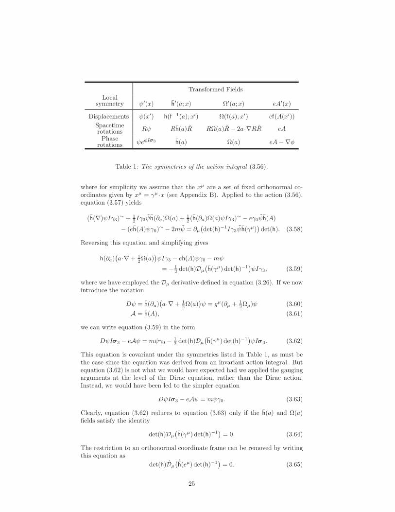
The action (3.56) is invariant under the symmetry transformations listed inTable 1.

3.4 The coupled Dirac equation

Having arrived at the action (3.56) we now derive the coupled Dirac equationby extremising with respect to ψ, treating all other fields as external. Whenapplying the Euler–Lagrange equations to the action (3.56) the ψ and ψ fieldsare not treated as independent, as they often are in quantum theory. Instead,we just apply the rules for the multivector derivative discussed in Section 2.2and Appendix B. The Euler–Lagrange equations can be written in the form

∂ψL = ∂µ(∂ψ,µL) (3.57)

24

Transformed Fields

Localsymmetry ψ′(x) h

′(a;x) Ω′(a;x) eA′(x)

Displacements ψ(x′) h(f−1(a);x′) Ω(f(a);x′) ef(A(x′))

Spacetimerotations Rψ Rh(a)R RΩ(a)R− 2a·∇RR eA

Phaserotations ψeφIσ3 h(a) Ω(a) eA−∇φ

Table 1: The symmetries of the action integral (3.56).

where for simplicity we assume that the xµ are a set of fixed orthonormal co-ordinates given by xµ = γµ ·x (see Appendix B). Applied to the action (3.56),equation (3.57) yields

(h(∇)ψIγ3)∼ + 1

2Iγ3ψh(∂a)Ω(a) + 12 (h(∂a)Ω(a)ψIγ3)

∼ − eγ0ψh(A)

− (eh(A)ψγ0)∼ − 2mψ = ∂µ

(

det(h)−1Iγ3ψh(γµ))

det(h). (3.58)

Reversing this equation and simplifying gives

h(∂a)(

a·∇ + 12Ω(a)

)

ψIγ3 − eh(A)ψγ0 −mψ

= − 12 det(h)Dµ

(

h(γµ) det(h)−1)

ψIγ3, (3.59)

where we have employed the Dµ derivative defined in equation (3.26). If we nowintroduce the notation

Dψ = h(∂a)(

a·∇ + 12Ω(a)

)

ψ = gµ(∂µ + 12Ωµ)ψ (3.60)

A = h(A), (3.61)

we can write equation (3.59) in the form

DψIσ3 − eAψ = mψγ0 − 12 det(h)Dµ

(

h(γµ) det(h)−1)

ψIσ3. (3.62)

This equation is covariant under the symmetries listed in Table 1, as must bethe case since the equation was derived from an invariant action integral. Butequation (3.62) is not what we would have expected had we applied the gaugingarguments at the level of the Dirac equation, rather than the Dirac action.Instead, we would have been led to the simpler equation

DψIσ3 − eAψ = mψγ0. (3.63)

Clearly, equation (3.62) reduces to equation (3.63) only if the h(a) and Ω(a)fields satisfy the identity

det(h)Dµ(

h(γµ) det(h)−1)

= 0. (3.64)

The restriction to an orthonormal coordinate frame can be removed by writingthis equation as

det(h)Dµ( ˙h(eµ) det(h)−1

)

= 0. (3.65)

25

(It is not hard to show that the left-hand side of equation (3.65) is a covari-ant vector; later it will be identified as a contraction of the ‘torsion’ tensor).There are good reasons for expecting equation (3.65) to hold. Otherwise, theminimally-coupled Dirac action would not yield the minimally-coupled equation,which would pose problems for our use of action principles to derive the gaugedfield equations. We will see shortly that the demand that equation (3.65) holdsplaces a strong restriction on the form that the gravitational action can take.

Some further comments about the derivation of (3.62) are now in order. Thederivation employed only the rules of vector and multivector calculus applied toa ‘flat-space’ action integral. The derivation is therefore a rigorous application ofthe variational principle. This same level of rigour is not always applied whenderiving field equations from action integrals involving spinors. Instead, thederivations are often heuristic — |ψ〉 and 〈ψ| are treated as independent variablesand the 〈ψ| is just ‘knocked off’ the Lagrangian density to leave the desiredequation. Furthermore, the action integral given by many authors for the Diracequation in a gravitational background has an imaginary component [44, 45], inwhich case the status of the variational principle is unclear. To our knowledge,only Hehl & Datta [9] have produced a derivation that in any way matchesthe derivation produced here. Hehl & Datta also found an equation similarto (3.65), but they were not working within a gauge theory setup and so did notcomment on the consistency (or otherwise) of the minimal-coupling procedure.

3.5 Observables and covariant derivatives

As well as keeping everything within the real spacetime algebra , representingDirac spinors by elements of the even subalgebra offers many advantages whenforming observables. As described in Appendix A, observables are formed by thedouble-sided application of a Dirac spinor ψ to some combination of the fixedγµ frame vectors. So, for example, the charge current is given by J = ψγ0ψand the spin current by s = ψγ3ψ. In general, an observable is of the form

M = ψΓψ, (3.66)

where Γ is a constant multivector formed from the γµ. All observables areinvariant under phase rotations, so Γ must be invariant under rotations in theIσ3 plane. Hence Γ can consist only of combinations of γ0, γ3, Iσ3 and theirduals (formed by multiplying by I). An important point is that, in forming theobservable M , the Γ multivector is completely ‘shielded’ from rotations. This iswhy the appearance of the γ0 and γ3 vectors on the right-hand side of the spinorψ in the Dirac action (3.56) does not compromise Lorentz invariance, and doesnot pick out a preferred direction in space [21]. All observables are unchangedby rotating the γµ frame vectors to R0γµR0 and transforming ψ to ψR0. (Inthe matrix theory this corresponds to a change of representation.)

Under translations and rotations the observables formed in the above man-ner (3.66) inherit the transformation properties of the spinor ψ. Under transla-tions the observable M = ψΓψ therefore transforms from M(x) to M(x′), andunder rotations M transforms to RψΓψR = RMR. The observable M is there-fore covariant. These Dirac observables are the first examples of quantities thattransform covariantly under rotations, but do not inherit this transformationlaw from the h-field. In contrast, all covariant forms of classical fields, such as

26

F or the covariant velocity along a worldline h−1(x), transform under rotations

in a manner that that is dictated by their coupling to the h-field. Classicalgeneral relativity in fact removes any reference to the rotation gauge from mostaspects of the theory. Quantum theory, however, demands that the rotationgauge be kept in explicitly and, as we shall show in Section 8, Dirac fields probethe structure of the gravitational fields at a deeper level than classical fields.Furthermore, it is only through consideration of the quantum theory that onereally discovers the need for the rotation-gauge field.

One might wonder why the observables are invariant under phase rotations,but only covariant under spatial rotations. In fact, the h-field enables us to formquantities like h(M), which are invariant under spatial rotations. This gives analternative insight into the role of the h-field. We will find that both covariantobservables (M) and their rotationally-invariant forms (h(M) and h

−1(M)) playimportant roles in the theory constructed here.

If we next consider the directional derivative of M , we find that it can bewritten as

∂µM = (∂µψ)Γψ + ψΓ(∂µψ)∼. (3.67)

This immediately tells us how to turn the directional derivative ∂µM into a co-variant derivative: simply replace the spinor directional derivatives by covariantderivatives. Hence we form

(Dµψ)Γψ + ψΓ(Dµψ)∼ = (∂µψ)Γψ + ψΓ(∂µψ)∼ + 12ΩµψΓψ − 1

2ψΓψΩµ

= ∂µ(ψΓψ) + Ωµ×(ψΓψ). (3.68)

We therefore recover the covariant derivative for observables:

DµM = ∂µM + Ωµ×M. (3.69)

This derivation shows that many features of the ‘classical’ derivation of gravi-tational gauge fields can be viewed as arising from more basic quantum trans-formation laws.

Throughout this section we have introduced a number of distinct gravita-tional covariant derivatives. We finish this section by discussing some of theirmain features and summarising our conventions. The operator Dµ acts on anycovariant multivector and has the important property of being a derivation, thatis it acts as a scalar differential operator,

Dµ(AB) = (DµA)B +A(DµB). (3.70)

This follows from Leibniz’ rule and the identity

Ωµ×(AB) = Ωµ×AB +AΩµ×B. (3.71)

Neither Dµ or Dµ are fully covariant, however, since they both contain the Ωµfield, which picks up a term in f under displacements (3.33). It is important inthe applications to follow that we work with objects that are covariant underdisplacements, and to this end we define

ω(a) = Ω(h(a)) = a·gµΩµ. (3.72)

27

Gauge fieldsDisplacements: h(a)

Rotations: Ω(a), ω(a) = Ω(h(a))

Spinor derivativesDµψ = ∂µψ + 1

2Ωµψ

a·Dψ = a·h(∇)ψ + 12ω(a)ψ

Observables derivatives

DµM = ∂µM + Ωµ×Ma·DM = a·h(∇)M + ω(a)×MDM = ∂aa·DM = D·M + D∧M

Vector derivative ∇ = eµ∂

∂xµ

Multivector derivative ∂X =∑

i<···<j

ei∧· · ·∧ej (ej∧· · ·∧ei)∗∂X

Table 2: Definitions and conventions

We also define the full covariant directional derivatives a·D and a·D by

a·Dψ = a·h(∇)ψ + 12ω(a)ψ (3.73)

a·DM = a·h(∇)M + ω(a)×M. (3.74)

Note that these conventions imply that Dµ = gµ·D, with a similar result holdingfor Dµ.

For the a·D operator we can further define the covariant vector derivative

DM = ∂a a·DM = gµDµM. (3.75)

The covariant vector derivative contains a grade-raising and a grade-loweringcomponent, so that

DA = D·A+ D∧A, (3.76)

where

D·A = ∂a ·(a·DA) = gµ ·(DµA) (3.77)

D∧A = ∂a∧(a·DA) = gµ∧(DµA). (3.78)

As with the vector derivative, D inherits the algebraic properties of a vector.A summary of our definitions and conventions is contained in Table 2. We

have endeavoured to keep these conventions as simple and natural as possible,but a word is in order on our choices. It should be clear that it is a goodidea to use a separate symbol for the spacetime vector derivative (∇), as op-posed to writing it as ∂x. This maintains a clear distinction between spacetimederivatives, and operations on linear functions such as ‘contraction’ (∂a·) and‘protraction’ (∂a∧). It is also useful to distinguish between spinor and vector

28

covariant derivatives, which is why we have introduced separate D and D sym-bols. We have avoided use of the d symbol, which already has a very specificmeaning in the language of differential forms. It is necessary to distinguish be-tween rotation-gauge derivatives (Dµ) and the full covariant derivative with theh-field included (a·D). Using Dµ and a·D for these achieves this separation inthe simplest possible manner. Throughout this paper we will switch betweenusing coordinate frames (as in Dµ) and the frame-free notation (such as ω(a)).Seeing which notation is appropriate for a given problem is something of an art,though we hope to convey some of the basic rules in what follows.

4 The field equations

Having introduced the h and Ω-fields, we now look to construct an invariantaction integral that will provide a set of gravitational field equations. We startby defining the field-strength via

[Dµ, Dν ]ψ = 12Rµνψ, (4.1)

so thatRµν = ∂µΩν − ∂νΩµ + Ωµ×Ων . (4.2)

It follows that we also have

[Dµ,Dν ]M = Rµν×M. (4.3)

A frame-free notation is introduced by writing

Rµν = R(eµ∧eν). (4.4)

The field R(a ∧ b) is a bivector-valued linear function of its bivector argumenta ∧ b. Its action on bivectors extends by linearity to the function R(B), whereB is an arbitrary bivector and therefore, in four dimensions, not necessarily apure ‘blade’ a∧ b. Where required, the position dependence is made explicit bywriting R(B;x).

Under an arbitrary rotation, the definition (4.2) ensures that R(B) trans-forms as

R(B) 7→ R′(B) = RR(B)R. (4.5)

Under local displacements we find that

R′(eµ∧eν) = ∂µΩ

′(eν) − ∂νΩ′(eµ) + Ω′(eν)×Ω′(eµ)

= f(eµ)·∇x′Ω(

f(eν);x′)

− f(eν)·∇x′Ω(

f(eµ);x′)

+ Ω′(eµ)×Ω′(eν)

+ Ω(

∂µf(eν) − ∂ν f(eµ);x′)

= R(

f(eµ∧eν);x′)

+ Ω(

∂µf(eν) − ∂ν f(eµ);x′)

. (4.6)

But we know that

∂µf(eν) − ∂ν f(eµ) = ∂µ∂νf(x) − ∂ν∂µf(x) = 0, (4.7)

so the field strength has the simple displacement transformation law

R(B) 7→ R′(B) = R

(

f(B);x′)

. (4.8)

29

A covariant quantity can therefore be constructed by defining

R(B) = R(h(B)). (4.9)

Under arbitrary displacements and local rotations, R(B) has the following trans-formation laws:

Translations: R′(B;x) = R(B;x′)

Rotations: R′(B) = RR(RBR) R.(4.10)

We refer to any linear function with transformation laws of this type as a co-variant tensor. R(B) is our gauge theory analogue of the Riemann tensor. Wehave started to employ a notation that is very helpful for the theory developedhere. Certain covariant quantities, such as R(B) and D, are written with cal-ligraphic symbols. This helps keep track of the covariant quantities and oftenenables a simple check that a given equation is gauge covariant. It is not nec-essary to write all covariant objects with calligraphic symbols, but it is helpfulfor common objects such as R(B) and D.

From R(B) we define the following contractions:

Ricci Tensor: R(b) = ∂a ·R(a∧b) (4.11)

Ricci Scalar: R = ∂a ·R(a) (4.12)

Einstein Tensor: G(a) = R(a) − 12aR. (4.13)

The argument of R determines whether it represents the Riemann or Riccitensors or the Ricci scalar. Furthermore, we never apply the extension notationof equation (2.50) to R(a), so R(a ∧ b) unambiguously denotes the Riemanntensor. Both R(a) and G(a) are also covariant tensors, since they inherit thetransformation properties of R(B).

The Ricci scalar is invariant under rotations, making it our first candidatefor a Lagrangian for the gravitational gauge fields. We therefore suppose thatthe overall action integral is of the form

S =

∫

|d4x| det(h)−1(12R− κLm), (4.14)

where Lm describes the matter content and κ = 8πG. The independent dynam-ical variables are h(a) and Ω(a), and in terms of these

R =⟨

h(∂b∧∂a)(

a·∇Ω(b) − b·∇Ω(a) + Ω(a)×Ω(b))⟩

. (4.15)

We also assume that Lm contains no second-order derivatives, so that h(a) andΩ(a) appear undifferentiated in the matter Lagrangian.

4.1 The h-equation

The h-field is undifferentiated in the entire action, so its Euler–Lagrange equa-tion is simply

∂h(a)(det(h)−1(R/2 − κLm)) = 0. (4.16)

Employing some results from Appendix B, we find that

∂h(a) det(h)−1 = − det(h)−1h−1(a) (4.17)

30

and

∂h(a)R = ∂

h(a)〈h(∂c∧∂b)R(b∧c)〉= 2h(∂b)·R(b∧a), (4.18)

so that∂h(a)(Rdet(h)−1) = 2G(h−1(a)) det(h)−1. (4.19)

If we now define the covariant matter stress-energy tensor T (a) by

det(h)∂h(a)(Lm det(h)−1) = T (h−1(a)), (4.20)

we arrive at the equationG(a) = κT (a). (4.21)

This is the gauge theory statement of Einstein’s equation. Note, however, thatas yet nothing should be assumed about the symmetry of G(a) or T (a). Inthis derivation only the gauge fields have been varied, and not the propertiesof spacetime. Therefore, despite the formal similarity with the Einstein equa-tions of general relativity, there is no doubt that we are still working in a flatspacetime.

4.2 The Ω-equation

The Euler–Lagrange field equation from Ω(a) is, after multiplying through bydet(h),

∂Ω(a)R− det(h)∂b ·∇(

∂Ω(a),bRdet(h)−1

)

= 2κ∂Ω(a)Lm, (4.22)

where we have made use of the assumption that Ω(a) does not contain anycoupling to matter through its derivatives. The derivatives ∂Ω(a) and ∂Ω(a),b

aredefined in Appendix B. The only properties required for this derivation are thefollowing:

∂Ω(a)〈Ω(b)M〉 = a·b〈M〉2 (4.23)

∂Ω(b),a〈c·∇Ω(d)M〉 = a·c b·d〈M〉2. (4.24)

From these we derive

∂Ω(a)〈h(∂d∧∂c)Ω(c)×Ω(d)〉 = Ω(d)×h(∂d∧a) + h(a∧∂c)×Ω(c)

= 2Ω(b)×h(∂b∧a) (4.25)

and

∂Ω(a),b

⟨

h(∂d∧∂c)(

c·∇Ω(d) − d·∇Ω(c))⟩

= h(a∧b) − h(b∧a)= 2h(a∧b). (4.26)

The right-hand side of (4.22) defines the ‘spin’ of the matter,

S(a) = ∂Ω(a)Lm, (4.27)

where S(a) is a bivector-valued linear function of a. Combining (4.22), (4.25)and (4.26) yields

h(∇)∧h(a) + det(h)∂b ·∇(

h(b) det(h)−1)

∧h(a)

+ Ω(∂b)×h(b∧a) = κS(a). (4.28)

31

Recall that in an expression such as this, the vectors a and b are viewed as beingindependent of position.

To make further progress we contract equation (4.28) with h−1(∂a). To

simplify this we require the result

〈b·∇h(a)h−1(∂a)〉 = det(h)−1〈b·∇h(∂a) ∂h(a) det(h)〉= det(h)−1b·∇det(h). (4.29)

We then obtain

−2 det(h)∂b ·∇(

h(b) det(h)−1)

− 2Ω(∂b)·h(b) = κh−1(∂a)·S(a). (4.30)

To convert this into its manifestly covariant form we first define the covariantspin tensor S(a) by

S(a) = S(

h−1(a)

)

. (4.31)

We can now write

det(h)Dµ( ˙h(eµ) det(h)−1

)

= − 12κ∂a ·S(a). (4.32)

In Section 3.3 we found that the minimally-coupled Dirac action gave rise tothe minimally-coupled Dirac equation only when the term on the left of thisequation was zero. We now see that this requirement amounts to the conditionthat the spin tensor has zero contraction. But, if we assume that the Ω(a) fieldonly couples to a Dirac fermion field, then the coupled Dirac action (3.56) gives

S(a) = S·a, (4.33)

where S is the spin trivector

S = 12ψIγ3ψ. (4.34)

In this case the contraction of the spin tensor does vanish:

∂a ·(S·a) = (∂a∧a)·S = 0. (4.35)

There is a remarkable consistency loop at work here. The Dirac action givesrise to a spin tensor of just the right type to ensure that the minimally-coupledaction produces the minimally-coupled equation. But this is only true if thegravitational action is given by the Ricci scalar ! No higher-order gravitationalaction is consistent in this way. So, if we demand that the minimally-coupledfield equations should be derivable from an action principle, we are led to ahighly constrained theory. This rules out, for example, the type of ‘R + R2’Lagrangian often considered in the context of Poincare gauge theory [46, 47,48]. In addition, the spin sector is also tightly constrained. Satisfyingly, theseconstraints force us to a theory that is first-order in the derivatives of the fields,keeping the theory on a similar footing to the Dirac and Maxwell theories.

The only freedom in the action for the gravitational fields is the possible in-clusion of a cosmological constant Λ. This just enters the action integral (4.14)as the term −Λ det(h)−1. The presence of such a term does not alter equa-tion (4.28), but changes (4.21) to

G(a) − Λa = κT (a). (4.36)

32

The presence of a cosmological constant cannot be ruled out on theoreticalgrounds alone, and this constant will be included when we consider applicationsto cosmology.

Given that the spin is entirely of Dirac type, equation (4.28) now takes theform

D∧h(a) = ∂b∧(b·Dh(a)) = κS·h(a). (4.37)

This is the second of our gravitational field equations. Between them, equa-tions (4.21) and (4.37) define a set of 40 scalar equations for the 40 unknownsin h(a) and Ω(a). Both equations are manifestly covariant. In the spin-torsionextension of general relativity (the Einstein–Cartan–Sciama–Kibble theory),D ∧ h(a) would be identified as the gravitational torsion, and equation (4.37)would be viewed as identifying the torsion with the matter spin density. Ofcourse, in GTG torsion is not a property of the underlying spacetime, it simplyrepresents a feature of the gravitational gauge fields. Equation (4.37) generalisesto the case of an arbitrary vector a = a(x) as follows:

D∧h(a) = h(∇∧a) + κS·h(a). (4.38)

Of particular use is the case where a is the coordinate frame vector eµ, so thatwe can write

D∧gµ = κS·gµ. (4.39)

4.3 Covariant forms of the field equations

For all the applications considered in this paper the gravitational fields aregenerated by matter fields with vanishing spin. So, to simplify matters, wehenceforth set S to zero and work with the second of the field equations in theform

D∧h(a) = h(∇∧a). (4.40)

It is not hard to make the necessary generalisations in the presence of spin.Indeed, even if the spin-torsion sector is significant, one can introduce a newfield [49]

ω′(a) = ω(a) − 12κa·S (4.41)

and then the modified covariant derivative with ω(a) replaced by ω′(a) stillsatisfies equation (4.40).

The approach we adopt in this paper is to concentrate on the quantitiesthat are covariant under displacements. Since both h(∇) and ω(a) satisfy thisrequirement, these are the quantities with which we would like to express thefield equations. To this end we define the operator

La = a·h(∇) (4.42)

and, for the remainder of this section, the vectors a, b etc. are assumed to bearbitrary functions of position. From equation (4.40) we write

h(∇)∧ ˙h(c) = −∂d∧

(

ω(d)·h(c))

=⇒ 〈b∧a h(∇)∧ ˙h(c)〉 = −

⟨

b∧a ∂d∧(

ω(d)·h(c))⟩

=⇒(

Lah(b) − Lbh(a))

·c =(

a·ω(b)− b·ω(a))

·h(c) (4.43)

33

where, as usual, the overdots determine the scope of a differential operator. Itfollows that the commutator of La and Lb is

[La, Lb] =(

Lah(b) − Lbh(a))

·∇=(

Lah(b) − Lbh(a))

·∇ + (Lab − Lba)·h(∇)

=(

a·ω(b) − b·ω(a) + Lab− Lba)

·h(∇). (4.44)

We can therefore write[La, Lb] = Lc, (4.45)

wherec = a·ω(b) − b·ω(a) + Lab− Lba = a·Db− b·Da. (4.46)

This ‘bracket’ structure summarises the intrinsic content of (4.37).The general technique we use for studying the field equations is to let ω(a)

contain a set of arbitrary functions, and then use (4.46) to find relations betweenthem. Fundamental to this approach is the construction of the Riemann tensorR(B), which contains a great deal of covariant information. From the definitionof the Riemann tensor (4.2) we find that

R(a∧b) = LaΩ(h(b)) − LbΩ(h(a)) + ω(a)×ω(b)

= Laω(b) − Lbω(a) + ω(a)×ω(b)− Ω(Lah(b) − Lbh(a)), (4.47)

henceR(a∧b) = Laω(b) − Lbω(a) + ω(a)×ω(b)− ω(c), (4.48)

where c is given by equation (4.46). Equation (4.48) now enables R(B) to becalculated in terms of position-gauge covariant variables.

Solution of the ‘wedge’ equation

Equation (4.40) can be solved to obtain ω(a) as a function of h and its deriva-tives. We define

H(a) = h(∇∧ ˙h−1(a)) = −h(∇)∧ ˙

h h−1(a), (4.49)

so that equation (4.40) becomes

∂b∧(ω(b)·a) = H(a). (4.50)

We solve this by first ‘protracting’ with ∂a to give

∂a∧∂b∧(ω(b)·a) = 2∂b∧ω(b) = ∂b∧H(b). (4.51)

Now, taking the inner product with a again, we obtain

ω(a) − ∂b∧(a·ω(b)) = 12a·(∂b∧H(b)). (4.52)

Hence, using equation (4.50) again, we find that

ω(a) = −H(a) + 12a·(∂b∧H(b)). (4.53)

In the presence of spin the term 12κa·S is added to the right-hand side.

34

4.4 Point-particle trajectories

The dynamics of a fermion in a gravitational background are described by theDirac equation (3.63) together with the quantum-mechanical rules for construct-ing observables. For many applications, however, it is useful to work with clas-sical and semi-classical approximations to the full quantum theory. The fullderivation of the semi-classical approximation is described in [34], but the es-sential idea is to specialise to motion along a single streamline defined by theDirac current ψγ0ψ. Thus the particle is described by a trajectory x(λ), to-gether with a spinor ψ(λ) which contains information about the velocity andspin of the particle. The covariant velocity is h

−1(x′) where, for this and thefollowing subsection, dashes are used to denote the derivative with respect to λ.The covariant velocity is identified with ψγ0ψ and the Lagrange multiplier p isincluded in the action integral to enforce this identification. Finally, an einbeine is introduced to ensure reparameterisation invariance. The resultant action is

S =

∫

dλ 〈ψ′Iσ3ψ + 12Ω(x′)ψIσ3ψ + p(v −meψγ0ψ) +m2e〉, (4.54)

wherev = h

−1(x′). (4.55)

The equations of motion arising from (4.54) are discussed elsewhere [34]. (Aneffect worth noting is that, due to the spin of the particle, the velocity v andmomentum p are not collinear.)

We can make a full classical approximation by neglecting the spin (droppingall the terms containing ψ) and replacing ψγ0ψ by p/m. This process leads tothe action

S =

∫

dλ(

p·h−1(x′) − 12e(p

2 −m2))

. (4.56)

The equations of motion derived from (4.56) are

v = ep (4.57)

p2 = m2 (4.58)

∂λh−1(p) = ∇p·h−1(x′). (4.59)

The final equation yields

∂λp = h(∇) p·h−1(x′) − x′ ·∇ h( ˙h−1(p)

)

= h(

(∇∧ ˙h−1(p))·h(v)

)

= H(p)·v (4.60)

where H(a) is defined by equation (4.49) and we have used equation (2.52).From equation (4.53) we see that a·ω(a) = −a·H(a), hence

e∂λ(v/e) = −ω(v)·v. (4.61)

This is the classical equation for a point-particle trajectory. It takes its simplestform when λ is the proper time τ along the trajectory. In this case e = 1/mand the equation becomes

∂v

∂τ= −ω(v)·v, (4.62)

35

or, in manifestly covariant form,

v ·D v = 0. (4.63)

This equation applies equally for massive particles (v2 = 1) and photons (v2 =0). Since equation (4.63) incorporates only gravitational effects, any deviationof v ·D v from zero can be viewed as the particle’s acceleration and must resultfrom additional external forces.

Equation (4.63) is usually derived from the action

S = m

∫

dλ√

h−1(x′)2 = m

∫

dλ

(

gµν∂xµ

∂λ

∂xν

∂λ

)1/2

, (4.64)

which is obtained from (4.56) by eliminating p and e with their respective equa-tions of motion. A Hamiltonian form such as (4.56) is rarely seen in conventionalgeneral relativity, since its analogue would require the introduction of a vier-bein. Despite this, the action (4.56) has many useful features, especially when itcomes to extracting conservation laws. For example, contracting equation (4.59)with a constant vector a yields

∂λ(

a·h−1(p))

= a·∇ p·h−1(x′). (4.65)

It follows that, if the h-field is invariant under translations in the direction a,then the quantity a · h−1(p) is conserved. In Section 5.5 we show that this resultextends to the case where h

−1(a) is a Killing vector.

4.5 The equivalence principle and the Newtonian limit

In the preceeding section we derived the equation v ·D v = 0 from the classicallimit of the Dirac action. This equation is the GTG analogue of the geodesicequation (see Appendix C). Arriving at such an equation shows that GTGembodies the weak equivalence principle — the motion of a test particle in agravitational field is independent of its mass. The derivation also shows thelimitations of this result, which only applies in the classical, spinless approxi-mation to quantum theory. The strong equivalence principle, that the laws ofphysics in a freely-falling frame are (locally) the same as those of special relativ-ity, is also embodied in GTG through the application of the minimal couplingprocedure. Indeed, it is clear that both of these ‘principles’ are the result ofthe minimal coupling procedure. Minimal coupling ensures, through the Diracequation, that point-particle trajectories are independent of particle mass in theabsence of other forces. It also tells us how the gravitational fields couple to anymatter field. As we have seen, this principle, coupled with the requirement ofconsistency with an action principle, is sufficient to specify the theory uniquely(up to an unspecified cosmological constant).

The relationship between the minimal coupling procedure (the gauge princi-ple) and the equivalence principle has been widely discussed previously. Feyn-man [50], for example, argues that a more exact version of the equivalencebetween linear acceleration and a gravitational field requires an equation of theform

gravity′ = gravity + acceleration, (4.66)

36

which clearly resembles a gauge transformation. What is not often stressed isthe viewpoint presented here, which is that if gravity is constructed entirelyas a gauge theory, there is no need to invoke the equivalence principle; thephysical effects embodied in the principle are simply consequences of the gaugetheory approach. This further illustrates the different conceptual foundationsof GTG and general relativity. Similarly, there is no need for the principleof general covariance in GTG, which is replaced by the requirement that allphysical predictions be gauge-invariant. It is often argued that the principleof general covariance is empty, because any physical theory can be written ina covariant form. This objection cannot be levelled at the statement that allphysical predictions must be gauge invariant, which has clear mathematical andphysical content.

The simplest, classical measurements in GTG are modelled by assumingthat observers can be treated as frames attached to a single worldline. If thisworldline is written as x(λ), then the covariant velocity is v = h

−1(x′), andthe affine parameter for the trajectory is that which ensures that v2 = 1. Theaffine parameter models the clock time for an observer on this trajectory. Ofcourse, there are many hidden assumptions in adopting this as a realistic model— quantum effects are ignored, as is the physical extent of the observer — butis is certainly a good model in weak fields. In strong fields a more satisfactorymodel would involve solving the Dirac equation to find the energy levels of anatom in the gravitational background and use this to model an atomic clock.

Equation (4.63) enables us to make classical predictions for freely-falling tra-jectories in GTG, and the photon case (v2 = 0) can be used to model signallingbetween observers. As an example, consider the formula for the redshift inducedby the gravitational fields. Suppose that a source of radiation follows a world-line x1(τ1), with covariant velocity v1 = h

−1(x′1). The radiation emitted followsa null trajectory with covariant velocity u (u2 = 0). This radiation is receivedby an observer with a worldline x2(τ2) and covariant velocity v2 = h

−1(x′2).The spectral shift z is determined by the ratio of the frequency observed at thesource, u(x1)·v1, and the frequency observed at the receiver, u(x2)·v2, by

1 + z =u(x1)·v1u(x2)·v2

. (4.67)

This quantity is physically observable since the right-hand side is a gauge-invariant quantity. This is because each of the four vectors appearing in (4.67)is covariant, which eliminates any dependence on position gauge, and taking thedot product between pairs of vectors eliminates any dependence on the rotationgauge.

A final point to address regarding the foundations of GTG is the recoveryof the Newtonian limit. Derivations of this are easily produced by adapting thestandard works in general relativity . Furthermore, in Section 6.3 we show thatthe description of the gravitational fields outside a static, spherically symmetricstar is precisely the same as in general relativity. The trajectories defined byequation (4.63) are those predicted by general relativity, so all of the predictionsfor planetary orbits (including those for binary pulsars) are unchanged. Simi-larly, the results for the bending of light are the same as in general relativity. Aswe show in the applications, any differences between GTG and general relativityemerge through the relationship with quantum theory, and through the globalnature of the gauge fields in GTG. These differences have no consequences for

37

classical tests of general relativity, though they are potentially testable throughthe interaction with quantum spin, and are certainly significant for discussingmore fundamental aspects of gravitational physics.

5 Symmetries, invariants and conservation laws

Having determined the gravitational gauge fields and their field equations, wenow establish some general results which are applied in the sections that follow.Again, we restrict to the case of vanishing torsion. The approach we adopt insolving the field equations is to let ω(a) be an arbitrary function, and then workwith a set of abstract first-order equations for the terms that comprise ω(a).However, in letting ω(a) be an arbitrary function, we lose some of the informa-tion contained in the ‘wedge’ equation (4.40). This information is recovered byenforcing various properties that the fields must satisfy, including the symmetryproperties of R(B) and the Bianchi identities. In addition, it is often necessaryto enforce some gauge-fixing conditions. For the rotation gauge these conditionsare applied by studying R(B), so it is important to analyse its general structure.

We start with the result that, for an arbitrary multivector A(x),

D∧(D∧A) = D∧(

h(∇∧h−1(A))

)

= h(∇∧∇∧h−1(A)) = 0, (5.1)

where we have made use of equation (4.40). It then follows from the result

gµ∧(

Dµ(gν∧(DνA)))

= gµ∧gν∧(DµDνA)

= 12 h(eµ)∧h(eν)∧(R(eµ∧eν)×A), (5.2)

that, for any multivector A,

∂a∧∂b∧(R(a∧b)×A) = 0. (5.3)

This derivation illustrates a useful point. Many derivations can be performedmost efficiently by working with the Dµ, since these contain commuting partialderivatives. However, the final expressions take their most transparent formwhen the h-field is included so that only fully covariant quantities are employed.

If we now set A in equation (5.3) equal to a vector c, and protract with ∂c,we find that

∂c∧∂a∧∂b∧(R(a∧b)×c) = −2∂a∧∂b∧R(a∧b) = 0. (5.4)

Taking the inner product of the term on the right-hand side with c we obtain

c·(

∂a∧∂b∧R(a∧b))

= ∂b∧R(c∧b) − ∂a∧R(a∧c) − ∂a∧∂b∧(R(a∧b)×c), (5.5)

in which both the left-hand side and the final term on the right-hand side vanish.We are therefore left with the simple expression

∂a∧R(a∧b) = 0, (5.6)

which summarises all the symmetries of R(B). This equation says that thetrivector ∂a ∧ R(a ∧ b) vanishes for all values of the vector b, so gives a setof 4 × 4 = 16 equations. These reduce the number of independent degrees offreedom in R(B) from 36 to the expected 20. It should be clear from the easewith which the degrees of freedom are calculated that the present geometricalgebra formulation has many advantages over traditional tensor calculus.

38

5.1 The Weyl tensor

A good example of the power of the present approach is provided by an analysisof the Riemann and Weyl tensors. To illustrate this point a number of examplesof R(B) for physical systems are included in this section. (These are stated herewithout derivation.) The first application of geometric algebra to the analysis ofthe Riemann tensor in classical differential geometry was given by Hestenes &Sobczyk [11, 15]. Here the formalism is developed and extended for applicationsrelevant to our gauge theory of gravity.

Six of the degrees of freedom in R(B) can be removed by arbitrary gaugerotations. It follows that R(B) can contain only 14 physical degrees of freedom.To see how these are encoded in R(B) we decompose it into Weyl and ‘matter’terms. Since the contraction of R(a ∧ b) results in the Ricci tensor R(a), weexpect that R(a∧b) will contain a term in R(a)∧b. This must be matched witha term in a∧R(b), since it is only the sum of these that is a function of a∧b.Contracting this sum we obtain

∂a ·(R(a)∧b+ a∧R(b)) = bR−R(b) + 4R(b) −R(b)

= 2R(b) + bR, (5.7)

and it follows that

∂a ·(

12 (R(a)∧b + a∧R(b)) − 1

6a∧bR)

= R(b). (5.8)

We can therefore write

R(a∧b) = W(a∧b) + 12

(

R(a)∧b + a∧R(b))

− 16a∧bR, (5.9)

where W(B) is the Weyl tensor, and must satisfy

∂a ·W(a∧b) = 0. (5.10)

Returning to equation (5.6) and contracting, we obtain

∂b ·(

∂a∧R(a∧b))

= ∂a∧R(a) = 0, (5.11)

which shows that the Ricci tensor R(a) is symmetric. It follows that

∂a∧(

12 (R(a)∧b+ a∧R(b)) − 1

6a∧bR)

= 0 (5.12)

and hence that∂a∧W(a∧b) = 0. (5.13)

Equations (5.10) and (5.13) combine to give the single equation

∂aW(a∧b) = 0. (5.14)

Since the ∂a· operation is called the ‘contraction’, and ∂a∧ the ‘protraction’,Hestenes & Sobczyk [11] have suggested that the sum of these be termed the‘traction’. Equation (5.9) thus decomposes R(B) into a ‘tractionless’ termW(B) and a term specified solely by the matter stress-energy tensor (whichdetermines R(a) through the Einstein tensor G(a)). There is no generally ac-cepted name for the part of R(B) that is not given by the Weyl tensor so, as itis entirely determined by the matter stress-energy tensor, we refer to it as thematter term.

39

5.2 Duality of the Weyl tensor

To study the consequences of equation (5.14) it is useful to employ the fixedγµ frame, so that equation (5.14) produces the four equations

σ1W(σ1) + σ2W(σ2) + σ3W(σ3) = 0 (5.15)

σ1W(σ1) − Iσ2W(Iσ2) − Iσ3W(Iσ3) = 0 (5.16)

−Iσ1W(Iσ1) + σ2W(σ2) − Iσ3W(Iσ3) = 0 (5.17)

−Iσ1W(Iσ1) − Iσ2W(Iσ2) + σ3W(σ3) = 0. (5.18)

Summing the final three equations, and using the first, produces

IσkW(Iσk) = 0 (5.19)

and substituting this into each of the final three equations produces

W(Iσk) = IW(σk). (5.20)

It follows that the Weyl tensor satisfies

W(IB) = IW(B), (5.21)

and so is ‘self-dual’. This use of the term ‘self-dual’ differs slightly from its usein the 2-spinor formalism of Penrose & Rindler [51]. However, the spacetimealgebra pseudoscalar I a similar role to the Hodge star operation (the dualitytransformation) in differential form theory, so ‘self-duality’ is clearly an appro-priate name for the relation expressed by equation (5.21).

The fact that tractionless linear functions mapping bivectors to bivectorsin spacetime satisfy equation (5.21) was first noted in [11]. Equation (5.21)means that W(B) can be analysed as a linear function on a three-dimensionalcomplex space rather as a function on a real six-dimensional space. This is whycomplex formalisms, such as the Newman–Penrose formalism, are so successfulfor studying vacuum solutions. The unit imaginary employed in the Newman–Penrose formalism is a disguised version of the spacetime pseudoscalar [33].Geometric algebra reveals the geometric origin of this ‘imaginary’ unit, andenables us to employ results from complex analysis without the need for formalcomplexification. Furthermore, the complex structure only arises in situationswhere it is geometrically significant, instead of being formally present in allcalculations.

Given the self-duality of the Weyl tensor, the remaining content of equations(5.15)–(5.18) is summarised by the relation

σkW(σk) = 0. (5.22)

This equation says that, viewed as a three-dimensional complex linear function,W(B) is symmetric and traceless. This gives W(B) five complex, or ten realdegrees of freedom. (Since we frequently encounter combinations of the formscalar + pseudoscalar, we refer to these loosely as ‘complex’ scalars.) The gauge-invariant information in W(B) is held in its complex eigenvalues and, since thesum of these is zero, only two are independent. This leaves a set of four realintrinsic scalar quantities.

40

Overall, R(B) has 20 degrees of freedom, 6 of which are contained in thefreedom to perform arbitrary local rotations. Of the remaining 14 physicaldegrees of freedom, four are contained in the two complex eigenvalues of W(B),and a further four in the real eigenvalues of the matter stress-energy tensor.The six remaining physical degrees of freedom determine the rotation betweenthe frame that diagonalises G(a) and the frame that diagonalises W(B). Thisidentification of the physical degrees of freedom contained in R(B) appears tobe new, and is potentially very significant.

5.3 The Petrov classification

The algebraic properties of the Weyl tensor are traditionally encoded in itsPetrov type. Here we present geometric algebra expressions for the main Petrovtypes (following the conventions of Kramer et al. [52]). The Petrov classificationis based on the solutions of the eigenvalue equation

W(B) = αB, (5.23)

in which B is a bivector (the ‘eigenbivector’) and α is a complex scalar. Thereare five Petrov types: I, II, III, D and N. Type I are the most general, with twoindependent eigenvalues and three linearly-independent orthogonal eigenbivec-tors. Such tensors have the general form

W(B) = 12α1(B + 3F1BF1) + 1

2α2(B + 3F2BF2) (5.24)

where α1 and α2 are complex scalars and F1 and F2 are orthogonal unit bivec-tors (F 2

1 = F 22 = 1). The eigenbivectors are F1, F2 and F3 = F1F2, and the

corresponding eigenvalues are (2α1 − α2), (2α2 − α1) and −(α1 + α2).Type D (degenerate) are a special case of type I tensors in which two of the

eigenvalues are the same. Physical examples are provided by the Schwarzschildand Kerr solutions. The region outside a spherically-symmetric source of massM has

R(B) = W(B) = − M

2r3(B + 3σrBσr) (5.25)

where σr is the unit radial bivector. The eigenbivectors of this function are σr,with eigenvalue −2M/r3, and any two bivectors perpendicular to σr, with eigen-value M/r3. Similarly, R(B) for a stationary axisymmetric source described bythe Kerr solution is [34, 53]

R(B) = W(B) = − M

2(r − IL cosθ)3(B + 3σrBσr). (5.26)

This differs from the radially-symmetric case (5.25) only in that its eigenvaluescontain an imaginary term governed by the angular momentum L. Verifyingthat (5.25) and (5.26) are tractionless is simple, requiring only the result that,for an arbitrary bivector B,

∂aFa∧b = ∂aF (ab− a·b) = −bF, (5.27)

which employs equation (2.40) from Section 2.2.The fact that the Riemann tensor for the Kerr solution is obtained from

that for the Schwarzschild solution by replacing r by r − IL cosθ is reminiscent

41

of a ‘trick’ used to derive the Kerr solution in the null tetrad formalism [54].This is particularly suggestive given that the unit imaginary employed in theNewman–Penrose formalism is a disguised version of the spacetime pseudoscalarI. The significance of these observations is discussed further in [55, 34].

For tensors of Petrov type other than I, null bivectors play a significantrole. Type II tensors have eigenvalues α1, −α1 and 0 and two independenteigenbivectors, one timelike and one null. Type III and type N have all threeeigenvalues zero, and satisfy

type III : W3(B) = 0, W2(B) 6= 0 (5.28)

type N : W2(B) = 0. (5.29)

An example of a type N tensor is provided by gravitational radiation. For aplane-polarised gravitational wave travelling in the γ3 direction R(B) is givenby

R+(B) = W+(B) = 14f(t− z) γ+(γ1Bγ1 − γ2Bγ2)γ+ (5.30)

for waves polarised in the direction of the γ1 and γ2 axes, and

R×(B) = W×(B) = 14f(t− z) γ+(γ1Bγ2 + γ2Bγ1)γ+ (5.31)

for waves polarised at 45 to the axes. In both cases f(t−z) is a scalar function,and γ+ is the null vector

γ+ = γ0 + γ3. (5.32)

The direct appearance of the null vector γ+ in W(B) shows that W2(B) = 0,and is physically very suggestive. Expressions of the type γ+Bγ+ project thebivector B down the null vector γ+, and such a structure is exhibited in theradiation field generated by an accelerating point charge [12].

These examples illustrate the uniquely compact forms for the Riemann ten-sor afforded by geometric algebra. In terms of both clarity and physical in-sight these expressions are far superior to any afforded by tensor algebra, theNewman–Penrose formalism or differential forms. Only Wahlquist and Es-tabrook’s (3+1) dyadic notation [56, 57] achieves expressions of comparablecompactness, although their formalism is of limited applicability.

5.4 The Bianchi identities

Further information from the wedge equation (4.40) is contained in the Bianchiidentity. One form of this follows from a simple application of the Jacobi iden-tity:

[Dα, [Dβ,Dγ ]]A+ cyclic permutations = 0 (5.33)

which implies that

DαR(eβ∧eγ) + cyclic permutations = 0. (5.34)

Again, use of the Dµ derivatives makes this identity straightforward, but morework is required to achieve a fully covariant relation.

We start by forming the adjoint relation to (5.34), which we can write as

∂a∧∂b∧∂c〈(

a·∇R(b∧c) + Ω(a)×R(b∧c))

B〉 = 0, (5.35)

42

where B is a constant bivector. We next need to establish the result that

B1 ·R(B2) = B2 ·R(B1). (5.36)

This follows by contracting equation (5.6) with an arbitrary vector and an ar-bitrary bivector to obtain the equations

∂c∧(a·R(c∧b)) = R(a∧b) (5.37)

(B ·∂a)·R(a∧b) = −∂aB ·R(a∧b). (5.38)

Protracting the second of these equations with ∂b and using the first, we obtain

∂b∧(

(B ·∂a)·R(a∧b))

= −2R(B) = −∂b∧∂aB ·R(a∧b). (5.39)

Taking the scalar product with a second bivector now gives equation (5.36).Using this result in equation (5.35), we now obtain

∇∧(

h−1(R(B))

)

− ∂a∧h−1(R(Ω(a)×B)) = 0. (5.40)

Finally, acting on this equation with h and using equation (4.40), we establishthe covariant result

D∧R(B) − ∂a∧R(ω(a)×B) = 0. (5.41)

This result takes a more natural form when B becomes an arbitrary function ofposition, and we write the Bianchi identity as

∂a∧(

a·DR(B) −R(a·DB))

= 0. (5.42)

We can extend the overdot notation of Section (2.2) in the obvious manner towrite equation (5.42) as

D∧R(B) = 0, (5.43)

which is very compact, but somewhat symbolic and hard to apply withoutunwrapping into the form of equation (5.42).

The self-duality of the Weyl tensor implies that

D∧W(I B) = −ID·W(B), (5.44)

so, in situations where the matter vanishes and W(B) is the only contributionto R(B), the Bianchi identities reduce to

DW(B) = 0. (5.45)

The properties of a first-order equation such as this are discussed in more detailin Section 7.1.

The contracted Bianchi identities are obtained from

(∂a∧∂b)·(

D∧R(a∧b))

= ∂a ·(

R(a∧D) + DR(a))

= 2R(D) −DR, (5.46)

from which we can writeG(D) = 0. (5.47)

An alternative form of this equation is obtained by taking the scalar productwith an arbitrary vector, and using the symmetry of G(a) to write

D·G(a) = 0. (5.48)

Written out in full, this equation takes the form

∂a ·(

LaG(b) − G(Lab) + ω(a)×G(b) − G(ω(a)×b))

= 0. (5.49)

43

5.5 Symmetries and conservation laws

We end this section with some comments on symmetries and conservation laws.These comments are not all directly relevant to the applications discussed inthis paper, but concern the general structure of GTG.

The first significant point is that the theory is founded on an action principlein a ‘flat’ vector space. It follows that all the familiar equations relating sym-metries of the action to conserved quantities hold without modification. (Thegeometric algebra approach to Lagrangian field theory is developed in [31, 34].)Any symmetry transformation of the total action integral that is parameterisedby a continuous scalar will result in a vector that is conserved with respect tothe vector derivative ∇. To every such vector there corresponds a covariantequivalent, as is seen from the simple rearrangement

D·J = ID∧(IJ )

= det(h)I∇∧(h−1(IJ ))

= det(h)∇·(h(J ) det(h)−1). (5.50)

So, if J satisfies ∇·J = 0, then the covariant equivalent

J = h−1(J) det(h) (5.51)

satisfies the covariant equation D·J = 0. (This explains the definition of Jin Section 3.2.) Note that if we attempt to form the canonical stress-energytensor conjugate to translations we obtain the quantity G(a)−κT (a), which thefield equations set to zero. The overall stress-energy tensor is therefore clearlyconserved, but this does not yield any new information.

A second feature of our use of flat background spacetime is that all differ-ential equations can be recast in integral form. The integral equation form isnot always useful, since it often forces one to deal with non-covariant quantities.But integral equations are particularly well-suited to handling singularities inthe gravitational fields. Just as Gauss’ theorem in electromagnetism can be usedto determine the structure of an electric field source, so integral equations canbe used to uncover the structure of the matter sources of gravitational fields.An example of this is provided in Section 6.4 where the Schwarzschild solution isshown to arise from a matter stress-energy tensor containing a single δ-functionsource of strength M . A less obvious example is contained in [55, 58], where itis shown that the matter generating the Kerr solution takes the form of a ringrotating at the speed of light, supported by a disk of tension. Such notions arequite different from classical general relativity.

Killing vectors have played a significant role in the analysis of symmetriesand conserved quantities in general relativity, and their properties are largelyunchanged in GTG. The simplest covariant form of Killing’s equation for aKilling vector K is that

a·(b·DK) + b·(a·DK) = 0 (5.52)

for any two vector fields a and b. Contracting with ∂a · ∂b immediately yieldsthe result that K is divergenceless:

D·K = 0. (5.53)

44

Killing vectors are frequently obtained when, in some coordinate system, themetric is independent of one of the coordinates. Suppose that gµν = gµ · gν isindependent of the x0 coordinate. It follows that

∂

∂x0gµν = gµ ·(g0 ·Dgν) + gν ·(g0 ·Dgµ) = 0. (5.54)

But, for a coordinate frame,

gµ ·Dgν − gν ·Dgµ = h−1(∂µeν − ∂νeµ) = 0 (5.55)

and using this in equation (5.54) we find that

gµ ·(gν ·DK) + gν ·(gµ ·DK) = 0, (5.56)

where K = g0. Equation (5.56) is entirely equivalent to the frame-free equa-tion (5.52).

A further consequence of equation (5.52) is that, for any vector a,

a·(a·DK) = 0. (5.57)

So, for a particle satisfying the geodesic equation v ·D v = 0 (4.63), we see that

∂τ (v ·K) = v ·D(v ·K) = K ·(v ·Dv) + v ·(v ·DK) = 0. (5.58)

It follows that the quantity v ·K is conserved along the worldline of a freely-falling particle.

45

Part II — Applications

46

6 Spherically-symmetric systems

The first full application of our formalism is to time-dependent spherically-symmetric fields. For simplicity, we consider only the case where the matteris described by a perfect fluid. The equations derived here are applicable tostatic and collapsing stars, radially-symmetric black holes and many aspects ofcosmology, including inflation. Furthermore, in a suitable gauge the relevantequations are essentially Newtonian in form, making their physical interpreta-tion quite transparent. Applications discussed here include an analytic solutionto the equations governing collapsing dust, and the new understanding of hori-zons forced by our gauge theory. This section includes an extended version ofthe work presented in [59].

6.1 The ‘intrinsic’ method

The traditional approach to solving the gravitational field equations is to startwith the metric gµν , which is usually encoded as a line element

ds2 = gµν dxµ dxν . (6.1)

The analogous quantity in GTG is derived from the h-function via

gµν = h−1(eµ)·h−1(eν), (6.2)

where the eµ comprise a coordinate frame (see also Appendix C). For a givenmatter stress-energy tensor, the field equations then yield a set of non-linear,second-order differential equations for the terms in gµν . These equations arenotoriously hard to solve. On the other hand, any metric is potentially a solu-tion to the Einstein equations — one where the matter stress-energy tensor isdetermined by the corresponding Einstein tensor. This approach, in which thetail wags the dog, has recently probably been more popular! Here we present anew approach to solving the gravitational field equations. The method is closelytied to our gauge-theoretic understanding of gravity, but can always be used togenerate a metric which solves the Einstein equations. So, even if one rejectsour gauge-theory description of gravity, the techniques developed below can stillbe viewed as providing a new method for studying the Einstein equations.

Under a local rotation the vector h−1(a) transforms as

h−1(a) 7→ Rh

−1(a)R. (6.3)

It follows that the metric gµν (6.2) is invariant under rotation-gauge transforma-tions. This is in keeping with our earlier observation that, at the classical level,it is possible to work with a set of equations that are invariant under rotation-gauge transformations, and this is precisely what general relativity does. Thisapproach has the advantage of removing a number of degrees of freedom fromthe theory, but one pays a heavy price for this: the equations become second-order and one has to deal with complicated non-linear terms. The approach wedevelop here is quite different. We keep the rotation-gauge field explicit, andwork entirely with quantities that transform covariantly under position-gaugetransformations. Such quantities include h(∇), ω(a) and R(B). We thereforework with directional derivatives of the form La = a · h(∇), and treat ω(a) as

47

an arbitrary field. The relationship between h(a) and ω(a) is then encoded inthe commutation relations of the La. This setup is achieved by initially makinga suitably general ansatz for the h-function. This trial form is then substi-tuted into equation (4.53) to find the general form of ω(a). An arbitrary ω(a)field consistent with this general form is then introduced, resulting in a set ofequations relating commutators of the La derivatives to the variables in ω(a).

Next, the Riemann tensor R(B) is constructed in terms of abstract first-order derivatives of the ω(a) and additional quadratic terms. The rotation-gauge freedom is then removed by specifying the precise form that R(B) takes.For example, one can arrange that W(B) is diagonal in a suitable frame. Thisgauge fixing is crucial in order to arrive at a set of equations that are notunder-constrained. With R(B) suitably fixed, one arrives at a set of relationsbetween first-order abstract derivatives of the ω(a), quadratic terms in ω(a),and matter terms. The final step is to impose the Bianchi identities, whichensure overall consistency of the equations with the bracket structure. Once allthis is achieved, one arrives at a fully ‘intrinsic’ set of equations. Solving theseequations usually involves searching for natural ‘integrating factors’. These in-tegrating factors provide ‘intrinsic’ coordinates, and many of the fields can beexpressed as functions of these coordinates alone. The final step is to ‘coordi-natise’ the solution by making an explicit (gauge) choice of the h-function. Thenatural way to do this is to ensure that the coordinates used in parameterisingh(a) match the intrinsic coordinates defined by the integrating factors.

The method outlined above is quite general and can be applied to a widerange of problems [34, 60, 61]. Here we employ it in the analysis of time-dependent spherically-symmetric systems.

6.2 The intrinsic field equations

We start by introducing a set of spherical polar coordinates. In terms of thefixed γµ frame we define:

t = x·γ0 cosθ = x·γ3/r

r =√

(x∧γ0)2 tanφ = (x·γ2)/(x·γ1).(6.4)

The associated coordinate frame is

et = γ0

er = x∧γ0 γ0/r

eθ = r cosθ(cosφγ1 + sinφγ2) − r sinθ γ3

eφ = r sinθ(− sinφγ1 + cosφγ2)

(6.5)

and the dual-frame vectors are denoted by et, er, eθ, eφ. We will also frequently

employ the unit vectors θ and φ defined by

θ = eθ/r, φ = eφ/(r sinθ). (6.6)

Associated with these unit vectors are the unit timelike bivectors

σr = eret, σθ = θet, σφ = φet, (6.7)

which satisfyσrσθσφ = eter θφ = I. (6.8)

48

The dual spatial bivectors are given by

Iσr = −θφ, Iσθ = erφ, Iσφ = −erθ. (6.9)

Throughout we use the abbreviations

∂r =∂

∂r, ∂t =

∂

∂t. (6.10)

The h-function

Our first step towards a solution is to decide on a general form of the h-functionthat is consistent with spherical symmetry. Suppose that B is a constant spatialbivector (et ·B = 0), and define

R = eB/2 (6.11)

x′ = RxR. (6.12)

Then, in analogy with electromagnetism, the gravitational fields will be spheri-cally symmetric if rotating h(a) to Rh(a)R and displacing it to the back-rotatedposition x′ leaves h(a) unchanged. Hence rotational symmetry is enforcedthrough the requirement that

Rhx′(RaR)R = h(a). (6.13)

This symmetry immediately implies that the er, et and eθ, eφ pairs decouple

from each other, and the action of h(a) on the θ and φ vectors is further restrictedto the form

h(θ) = αθ + βφ

h(φ) = αφ− βθ.(6.14)

However, the skew-symmetric term parameterised by β can always be removedby a rotation in the Iσr plane, so we can assume that h(a) is diagonal oneθ, eφ. No such assumption can be made for the er, et vectors, so we takeh(a) as having the general form

h(et) = f1et + f2e

r

h(er) = g1er + g2e

t

h(eθ) = αeθ

h(eφ) = αeφ,

(6.15)

where f1, f2, g1, g2 and α are all functions of t and r only. We retain the gaugefreedom to perform a boost in the σr direction, and this freedom is employedlater to simplify the equations. Our remaining position-gauge freedom lies inthe freedom to reparameterise t and r, which does not affect the general formof (6.15). A natural parameterisation will emerge once the ‘intrinsic’ variableshave been identified.

The ω-function

To find a general form ω(a) consistent with (6.15) we substitute equation (6.15)into equation (4.53) for ω(a) as a function of h(a). Where the coefficients contain

49

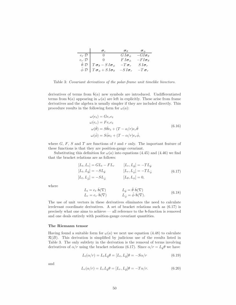
σr σθ σφ

et ·D 0 GIσφ −GIσθer ·D 0 F Iσφ −FIσθθ ·D T σθ − S Iσφ −T σr S Iσrφ·D T σφ + S Iσθ −S Iσr −T σr

Table 3: Covariant derivatives of the polar-frame unit timelike bivectors.

derivatives of terms from h(a) new symbols are introduced. Undifferentiatedterms from h(a) appearing in ω(a) are left in explicitly. These arise from framederivatives and the algebra is usually simpler if they are included directly. Thisprocedure results in the following form for ω(a):

ω(et) = Geret

ω(er) = Feret

ω(θ) = Sθet + (T − α/r)er θ

ω(φ) = Sφet + (T − α/r)erφ,

(6.16)

where G, F , S and T are functions of t and r only. The important feature ofthese functions is that they are position-gauge covariant.

Substituting this definition for ω(a) into equations (4.45) and (4.46) we findthat the bracket relations are as follows:

[Lt, Lr] = GLt − FLr [Lr, Lθ] = −TLθ[Lt, Lθ] = −SLθ [Lr, Lφ] = −TLφ[Lt, Lφ] = −SLφ [Lθ, Lφ] = 0,

(6.17)

whereLt = et ·h(∇) Lθ = θ ·h(∇)

Lr = er ·h(∇) Lφ = φ·h(∇).(6.18)

The use of unit vectors in these derivatives eliminates the need to calculateirrelevant coordinate derivatives. A set of bracket relations such as (6.17) isprecisely what one aims to achieve — all reference to the h-function is removedand one deals entirely with position-gauge covariant quantities.

The Riemann tensor

Having found a suitable form for ω(a) we next use equation (4.48) to calculateR(B). This derivation is simplified by judicious use of the results listed inTable 3. The only subtlety in the derivation is the removal of terms involvingderivatives of α/r using the bracket relations (6.17). Since α/r = Lθθ we have

Lt(α/r) = LtLθθ = [Lt, Lθ]θ = −Sα/r (6.19)

andLr(α/r) = LrLθθ = [Lr, Lθ]θ = −Tα/r. (6.20)

50

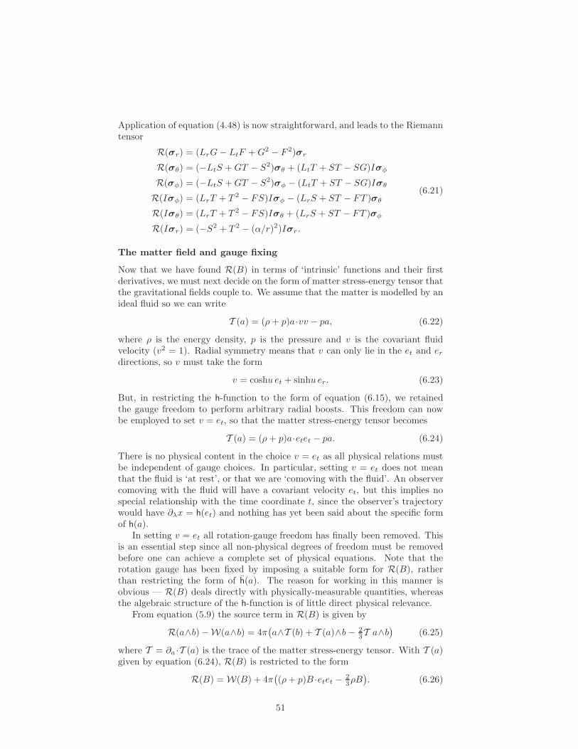
Application of equation (4.48) is now straightforward, and leads to the Riemanntensor

R(σr) = (LrG− LtF +G2 − F 2)σr

R(σθ) = (−LtS +GT − S2)σθ + (LtT + ST − SG)Iσφ

R(σφ) = (−LtS +GT − S2)σφ − (LtT + ST − SG)Iσθ

R(Iσφ) = (LrT + T 2 − FS)Iσφ − (LrS + ST − FT )σθ

R(Iσθ) = (LrT + T 2 − FS)Iσθ + (LrS + ST − FT )σφ

R(Iσr) = (−S2 + T 2 − (α/r)2)Iσr.

(6.21)

The matter field and gauge fixing

Now that we have found R(B) in terms of ‘intrinsic’ functions and their firstderivatives, we must next decide on the form of matter stress-energy tensor thatthe gravitational fields couple to. We assume that the matter is modelled by anideal fluid so we can write

T (a) = (ρ+ p)a·vv − pa, (6.22)

where ρ is the energy density, p is the pressure and v is the covariant fluidvelocity (v2 = 1). Radial symmetry means that v can only lie in the et and erdirections, so v must take the form

v = coshu et + sinhu er. (6.23)

But, in restricting the h-function to the form of equation (6.15), we retainedthe gauge freedom to perform arbitrary radial boosts. This freedom can nowbe employed to set v = et, so that the matter stress-energy tensor becomes

T (a) = (ρ+ p)a·etet − pa. (6.24)

There is no physical content in the choice v = et as all physical relations mustbe independent of gauge choices. In particular, setting v = et does not meanthat the fluid is ‘at rest’, or that we are ‘comoving with the fluid’. An observercomoving with the fluid will have a covariant velocity et, but this implies nospecial relationship with the time coordinate t, since the observer’s trajectorywould have ∂λx = h(et) and nothing has yet been said about the specific formof h(a).

In setting v = et all rotation-gauge freedom has finally been removed. Thisis an essential step since all non-physical degrees of freedom must be removedbefore one can achieve a complete set of physical equations. Note that therotation gauge has been fixed by imposing a suitable form for R(B), ratherthan restricting the form of h(a). The reason for working in this manner isobvious — R(B) deals directly with physically-measurable quantities, whereasthe algebraic structure of the h-function is of little direct physical relevance.

From equation (5.9) the source term in R(B) is given by

R(a∧b) −W(a∧b) = 4π(

a∧T (b) + T (a)∧b− 23T a∧b

)

(6.25)

where T = ∂a ·T (a) is the trace of the matter stress-energy tensor. With T (a)given by equation (6.24), R(B) is restricted to the form

R(B) = W(B) + 4π(

(ρ+ p)B ·etet − 23ρB

)

. (6.26)

51

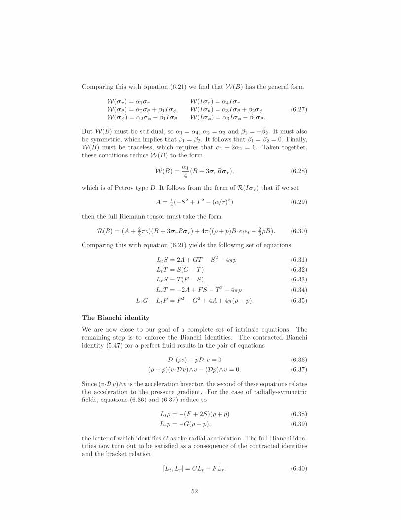
Comparing this with equation (6.21) we find that W(B) has the general form

W(σr) = α1σr W(Iσr) = α4IσrW(σθ) = α2σθ + β1Iσφ W(Iσθ) = α3Iσθ + β2σφ

W(σφ) = α2σφ − β1Iσθ W(Iσφ) = α3Iσφ − β2σθ.(6.27)

But W(B) must be self-dual, so α1 = α4, α2 = α3 and β1 = −β2. It must alsobe symmetric, which implies that β1 = β2. It follows that β1 = β2 = 0. Finally,W(B) must be traceless, which requires that α1 + 2α2 = 0. Taken together,these conditions reduce W(B) to the form

W(B) =α1

4(B + 3σrBσr), (6.28)

which is of Petrov type D. It follows from the form of R(Iσr) that if we set

A = 14 (−S2 + T 2 − (α/r)2) (6.29)

then the full Riemann tensor must take the form

R(B) = (A+ 23πρ)(B + 3σrBσr) + 4π

(

(ρ+ p)B ·etet − 23ρB

)

. (6.30)

Comparing this with equation (6.21) yields the following set of equations:

LtS = 2A+GT − S2 − 4πp (6.31)

LtT = S(G− T ) (6.32)

LrS = T (F − S) (6.33)

LrT = −2A+ FS − T 2 − 4πρ (6.34)

LrG− LtF = F 2 −G2 + 4A+ 4π(ρ+ p). (6.35)

The Bianchi identity

We are now close to our goal of a complete set of intrinsic equations. Theremaining step is to enforce the Bianchi identities. The contracted Bianchiidentity (5.47) for a perfect fluid results in the pair of equations

D·(ρv) + pD·v = 0 (6.36)

(ρ+ p)(v ·D v)∧v − (Dp)∧v = 0. (6.37)

Since (v·D v)∧v is the acceleration bivector, the second of these equations relatesthe acceleration to the pressure gradient. For the case of radially-symmetricfields, equations (6.36) and (6.37) reduce to

Ltρ = −(F + 2S)(ρ+ p) (6.38)

Lrp = −G(ρ+ p), (6.39)

the latter of which identifies G as the radial acceleration. The full Bianchi iden-tities now turn out to be satisfied as a consequence of the contracted identitiesand the bracket relation

[Lt, Lr] = GLt − FLr. (6.40)

52

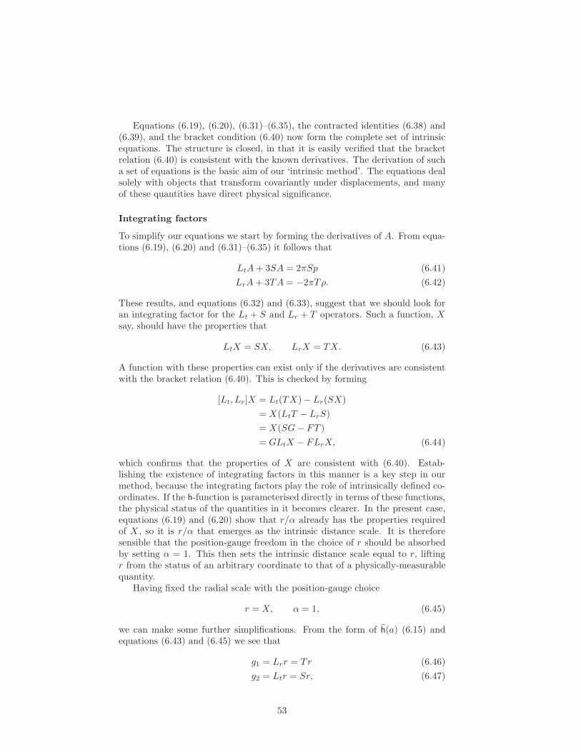
Equations (6.19), (6.20), (6.31)–(6.35), the contracted identities (6.38) and(6.39), and the bracket condition (6.40) now form the complete set of intrinsicequations. The structure is closed, in that it is easily verified that the bracketrelation (6.40) is consistent with the known derivatives. The derivation of sucha set of equations is the basic aim of our ‘intrinsic method’. The equations dealsolely with objects that transform covariantly under displacements, and manyof these quantities have direct physical significance.

Integrating factors

To simplify our equations we start by forming the derivatives of A. From equa-tions (6.19), (6.20) and (6.31)–(6.35) it follows that

LtA+ 3SA = 2πSp (6.41)

LrA+ 3TA = −2πTρ. (6.42)

These results, and equations (6.32) and (6.33), suggest that we should look foran integrating factor for the Lt + S and Lr + T operators. Such a function, Xsay, should have the properties that

LtX = SX, LrX = TX. (6.43)

A function with these properties can exist only if the derivatives are consistentwith the bracket relation (6.40). This is checked by forming

[Lt, Lr]X = Lt(TX)− Lr(SX)

= X(LtT − LrS)

= X(SG− FT )

= GLtX − FLrX, (6.44)

which confirms that the properties of X are consistent with (6.40). Estab-lishing the existence of integrating factors in this manner is a key step in ourmethod, because the integrating factors play the role of intrinsically defined co-ordinates. If the h-function is parameterised directly in terms of these functions,the physical status of the quantities in it becomes clearer. In the present case,equations (6.19) and (6.20) show that r/α already has the properties requiredof X , so it is r/α that emerges as the intrinsic distance scale. It is thereforesensible that the position-gauge freedom in the choice of r should be absorbedby setting α = 1. This then sets the intrinsic distance scale equal to r, liftingr from the status of an arbitrary coordinate to that of a physically-measurablequantity.

Having fixed the radial scale with the position-gauge choice

r = X, α = 1, (6.45)

we can make some further simplifications. From the form of h(a) (6.15) andequations (6.43) and (6.45) we see that

g1 = Lrr = Tr (6.46)

g2 = Ltr = Sr, (6.47)

53

which gives two of the functions in h(a). We also define

M = −2r3A = 12r(g2

2 − g12 + 1), (6.48)

which satisfiesLtM = −4πr2g2p (6.49)

andLrM = 4πr2g1ρ. (6.50)

The latter shows that M plays the role of an intrinsic mass.

The ‘Newtonian’ gauge

So far a natural distance scale has been identified, but no natural time coordinatehas emerged. To complete the solution it is necessary to make a choice for thet coordinate, so we now look for additional criteria to motivate this choice. Weare currently free to perform an arbitrary r and t-dependent displacement alongthe et direction. This gives us complete freedom in the choice of f2 function. Anindication of how this choice should be made is obtained from equations (6.49)and (6.50) for the derivatives of M (6.49), which invert to yield

∂M

∂t=

−4πg1g2r2(ρ+ p)

f1g1 − f2g2(6.51)

∂M

∂r=

4πr2(f1g1ρ+ f2g2p)

f1g1 − f2g2. (6.52)

The second equation reduces to a simple classical relation if we choose f2 = 0,as we then obtain

∂rM = 4πr2ρ, (6.53)

which says that M(r, t) is determined by the amount of mass-energy in a sphereof radius r. There are other reasons for choosing the time variable such thatf2 = 0. For example, we can then use the bracket structure to solve for f1.With f2 = 0 we have

Lt = f1∂t + g2∂r (6.54)

Lr = g1∂r, (6.55)

and the bracket relation (6.40) implies that

Lrf1 = −Gf1. (6.56)

It follows that

f1 = ǫ(t) exp

(

−∫ r

G/g1 dr

)

. (6.57)

The function ǫ(t) can be absorbed by a further t-dependent rescaling along et(which does not change f2), so with f2 = 0 we can reduce to a system in which

f1 = exp

(

−∫ r

G/g1 dr

)

. (6.58)

Another reason why f2 = 0 is a natural gauge choice is seen when the pressureis zero. In this case equation (6.39) forces G to be zero, and equation (6.58)

54

then forces f1 = 1. A free-falling particle with v = et (i.e. comoving with thefluid) then has

tet + rer = et + g2 er, (6.59)

where henceforth the dots denote differentiation with respect to the propertime. Since t = 1 the time coordinate t matches the proper time of all observerscomoving with the fluid. So, in the absence of pressure, we are able to recover aglobal ‘Newtonian’ time on which all observers can agree (provided all clocks arecorrelated initially). Furthermore it is also clear from (6.59) that g2 representsthe velocity of the particle. Hence equation (6.51), which reduces to

∂tM = −4πr2g2ρ (6.60)

in the absence of pressure, has a simple Newtonian interpretation — it equatesthe work with the rate of flow of energy density. Equation (6.48), written in theform

g22

2− M

r=g1

2 − 1

2, (6.61)

is also now familiar from Newtonian physics — it is a Bernoulli equation forzero pressure and total (non-relativistic) energy (g1

2 − 1)/2.For these reasons we refer to f2 = 0 as defining the ‘Newtonian’ gauge. The

applications discussed in the following sections vindicate our claim that thisis the natural gauge for radially-symmetric systems. The full set of equationsin the Newtonian gauge are summarised in Table 4. They underlie a widerange of phenomena in relativistic astrophysics and cosmology. The closestanalogue of the Newtonian gauge description of a spherically-symmetric systemis provided by Gautreau’s ‘curvature coordinates’ [62] (see also [63, 64]). Thisdescription employs a set of geodesic clocks in radial freefall, comoving withthe fluid. However, such a description can only be applied if the pressure isindependent of radius, whereas the Newtonian gauge description is quite general.

One aspect of the equations in Table 4 is immediately apparent. Given anequation of state p = p(ρ), and initial data in the form of the density ρ(r, t0)and the velocity g2(r, t0), the future evolution of the system is fully determined.This is because ρ determines p and M on a time slice, and the definition of Mthen determines g1. The equations for Lrp, Lrg1 and Lrg2 then determine theremaining information on the time slice. Finally, the LtM and Ltg2 equationscan be used to update the information to the next time slice, and the processcan then start again. The equations can thus be implemented numerically asa simple set of first-order update equations. This fact considerably simplifiesthe study of collapsing matter, and should be particularly significant in cur-rent studies of the critical phenomena associated with horizon and singularityformation [65, 66].

6.3 Static matter distributions

As a simple first application we consider a static, radially-symmetric matterdistribution. In this case ρ and p are functions of r only. Since M(r, t) is nowgiven by

M(r) =

∫ r

0

4πr′2ρ(r′) dr′ (6.62)

55

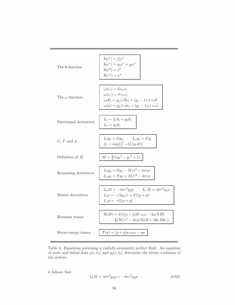
The h-function

h(et) = f1et

h(er) = g1er + g2e

t

h(eθ) = eθ

h(eφ) = eφ

The ω function

ω(et) = Geret

ω(er) = Feret

ω(θ) = g2/r θet + (g1 − 1)/r erθ

ω(φ) = g2/r φet + (g1 − 1)/r erφ

Directional derivativesLt = f1∂t + g2∂r

Lr = g1∂r

G, F and f1Ltg1 = Gg2, Lrg2 = Fg1

f1 = exp(∫ r −G/g1 dr

)

Definition of M M = 12r(g2

2 − g12 + 1)

Remaining derivativesLtg2 = Gg1 −M/r2 − 4πrp

Lrg1 = Fg2 +M/r2 − 4πrρ

Matter derivatives

LtM = −4πr2g2p, LrM = 4πr2g1ρ

Ltρ = −(2g2/r + F )(ρ+ p)

Lrp = −G(ρ+ p)

Riemann tensorR(B) = 4π

(

(ρ+ p)B ·etet − 2ρ/3B)

− 12 (M/r3 − 4πρ/3)(B + 3σrBσr)

Stress-energy tensor T (a) = (ρ+ p)a·etet − pa

Table 4: Equations governing a radially-symmetric perfect fluid. An equationof state and initial data ρ(r, t0) and g2(r, t0) determine the future evolution ofthe system.

it follows thatLtM = 4πr2g2ρ = −4πr2g2p. (6.63)

56

For any physical matter distribution ρ and p must both be positive, in whichcase equation (6.63) can be satisfied only if

g2 = F = 0. (6.64)

Since g2 = 0 we see that g1 is given simply in terms of M(r) by

g12 = 1 − 2M(r)/r, (6.65)

which recovers contact with the standard line element for a static, radially-symmetric field. It is immediately clear that a solution exists only if 2M(r) < rfor all r. This is equivalent to the condition that a horizon has not formed.

The remaining equation of use is that for Ltg2, which now gives

Gg1 = M(r)/r2 + 4πrp. (6.66)

Equations (6.65) and (6.66) combine with that for Lrp to give the famousOppenheimer–Volkov equation

∂p

∂r= − (ρ+ p)(M(r) + 4πr3p)

r(r − 2M(r)). (6.67)

At this point we have successfully recovered all the usual equations governinga non-rotating star, and the description is therefore unchanged from that ofstandard general relativity. The work involved in recovering these equationsfrom the full time-dependent case is minimal, and the final form of h(a) is verysimple (it is a diagonal function). Furthermore, the meaning of the t and rcoordinates is clear, since they have been defined operationally.

The solution extends straightforwardly to the region outside the star. Wenow have M constant, and

f1 = 1/g1 = (1 − 2M/r)−1/2, (6.68)

which recovers the Schwarzschild line element. It follows that all predictions forthe behaviour of matter in the star’s gravitational field, including those for thebending of light and the perihelion precession of Mercury, are unchanged.

6.4 Point source solutions — black holes

The next solution of interest is obtained when the matter is concentrated at asingle point (r = 0). For such a solution, ρ = p = 0 everywhere away from thesource, and the matter equations reduce to

LtM = 0LrM = 0

=⇒ M = constant. (6.69)

Retaining the symbol M for this constant we find that the equations reduce to

Ltg1 = Gg2 (6.70)

Lrg2 = Fg1 (6.71)

and

g12 − g2

2 = 1 − 2M/r. (6.72)

57

No further equations yield new information, so we have an under-determinedsystem of equations and some additional gauge fixing is needed to choose anexplicit form of h(a). The reason for this is that in the vacuum region theRiemann tensor reduces to

R(B) = − M

2r3(B + 3σrBσr). (6.73)

This tensor is now invariant under boosts in the σr plane, whereas previously thepresence of the fluid velocity in the Riemann tensor vector broke this symmetry.The appearance of this new symmetry in the matter-free case manifests itselfas a new freedom in the choice of h-function.

Given this new freedom, we should look for a choice of g1 and g2 that sim-plifies the equations. If we attempt to reproduce the Schwarzschild solution wehave to set g2 = 0, but then we immediately run into difficulties with g1, whichis not defined for r < 2M . We must therefore look for an alternative gaugechoice. We show in the following section that, when p = 0, g1 controls the en-ergy of infalling matter, with particles starting at rest at r = ∞ correspondingto g1 = 1. A sensible gauge choice is therefore to set

g1 = 1 (6.74)

so that

g2 = −√

2M/r (6.75)

G = 0 (6.76)

F = −M/(g2r2) (6.77)

and

f1 = 1. (6.78)

In this gauge the h-function takes the remarkably simple form

h(a) = a−√

2M/r a·er et, (6.79)

which only differs from the identity through a single term. From the results ofSection 2.3 the extension to the action of h on an arbitrary multivector A isstraightforward:

h(A) = A−√

2M/r(A·er)∧et. (6.80)

It follows that det(h) = 1 and the inverse of the adjoint function, as definedby (2.53), is given by

h−1(A) = A+

√

2M/r(A·et)∧er. (6.81)

Point-particle trajectories

To study the properties of the solution (6.79) we consider the equation of motionfor infalling matter. For a particle following the trajectory x(τ), with τ theproper time, we have

v = t et + (t√

2M/r + r)er + θeθ + φeφ, (6.82)

58

where dots denote the derivative with respect to τ . Since the h-function isindependent of t we have, from equation (4.65),

h−1(et)·v = (1 − 2M/r)t− r

√

2M/r = constant, (6.83)

and, for particles moving forwards in time (t > 0 for r → ∞), we can write

(1 − 2M/r)t = α+ r√

2M/r, (6.84)

where the constant α satisfies α > 0. The r equation is found from the constraintthat v2 = 1, which gives

r2 = α2 − (1 − 2M/r)(1 + r2(θ2 + sin2θ φ2)). (6.85)

The horizon lies at r = 2M since, for r < 2M , the velocity r must be negative.It might appear that an attempt to integrate equation (6.84) will run into diffi-culties with the pole at horizon, but this not the case. At r = 2M we find thatr = −α and this cancels the pole. All particles therefore cross the horizon andreach the singularity in a finite coordinate time.

Specialising to the case of radial infall, we see from equation (6.85) that theconstant α2 − 1 can be identified with twice the particle’s initial energy (fora unit mass particle). Furthermore, equation (6.85) shows immediately that rsatisfies

r = −M/r2, (6.86)

a feature of motion in a spherically-symmetric gravitational field that is rarelyemphasised in general relativity texts. Some possible matter and photon tra-jectories are illustrated in Figure 1. In the case where the particle is droppedfrom rest at r = ∞ equations (6.84) and (6.85) reduce to

r = −√

2M/r, t = 1, (6.87)

and we recover an entirely Newtonian description of the motion. The propertiesof a black hole are so simple in the gauge defined by (6.79) that it is astonish-ing that this gauge is almost never seen in the literature (see [67, 64] for someexceptions). Presumably, this is because the line element associated with (6.79)does not look as natural as the h-function itself and hides the underlying sim-plicity of the system. Part of the reason for this is that the line element is notdiagonal, and relativists usually prefer to find a coordinate system which diag-onalises gµν . Even when the freefall time coordinate t is employed, a differentradial coordinate is usually found to keep the metric diagonal [68, 69].

Since the gauge defined by g1 = 1 and g2 = −√

2M/r extends our aim ofkeeping the equations in a simple Newtonian form, we refer to this solutionas defining the ‘Newtonian gauge’ vacuum solution. We show in Section 6.5that this gauge arises naturally from the description of collapsing dust. Inthe Newtonian gauge one hardly needs to modify classical reasoning at all tounderstand the processes involved — all particles just cross the horizon andfall into the singularity in a finite coordinate time. And the horizon is locatedat r = 2M precisely because we can apply Newtonian arguments! The onlydepartures from Newtonian physics lie in relativistic corrections to the propertime taken for infall, and in modifications to the equations for angular motionwhich lead to the familiar results for orbital precession.

59

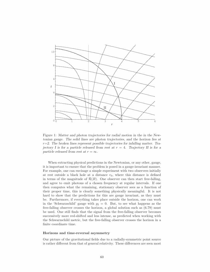
0

2

4

6

8

10

0 1 2 3 4 5 6r

tI

II

Figure 1: Matter and photon trajectories for radial motion in the in the New-tonian gauge. The solid lines are photon trajectories, and the horizon lies atr=2. The broken lines represent possible trajectories for infalling matter. Tra-jectory I is for a particle released from rest at r = 4. Trajectory II is for aparticle released from rest at r = ∞.

When extracting physical predictions in the Newtonian, or any other, gauge,it is important to ensure that the problem is posed in a gauge-invariant manner.For example, one can envisage a simple experiment with two observers initiallyat rest outside a black hole at a distance r0, where this distance is definedin terms of the magnitude of R(B). One observer can then start free-falling,and agree to emit photons of a chosen frequency at regular intervals. If onethen computes what the remaining, stationary observer sees as a function oftheir proper time, this is clearly something physically meaningful. It is nothard to show that the predictions for this are gauge invariant, as they mustbe. Furthermore, if everything takes place outside the horizon, one can workin the ‘Schwarzschild’ gauge with g2 = 0. But, to see what happens as thefree-falling observer crosses the horizon, a global solution such as (6.79) mustbe used. One still finds that the signal from the free-falling observer becomessuccessively more red-shifted and less intense, as predicted when working withthe Schwarzschild metric, but the free-falling observer crosses the horizon in afinite coordinate time.

Horizons and time-reversal asymmetry

Our picture of the gravitational fields due to a radially-symmetric point sourceis rather different from that of general relativity. These differences are seen most

60

clearly in the effects of time reversal. Time reversal is achieved by combiningthe displacement

f(x) = −etxet = x′ (6.88)

with the reflectionh′(a) = −eth(a)et, (6.89)

resulting in the the time-reversed solution

h∗(a) = ethx′(etaet)et. (6.90)

As an example, the identity function h(a) = a is time-reverse symmetric — as itshould be. The displacement (6.88) is a gauge transformation and cannot haveany physical consequences. The reflection (6.89) is not a gauge transformation,however, and can be used to transform between physically distinct gauge sectors.The reflection (6.89) is lost when the metric is formed, so general relativitycannot handle time-reversal in the same manner as GTG.

With the h-function described by equation (6.15), and with the fi andgi functions of r only, the effect of (6.90) is simply to change the sign of theoff-diagonal elements f2 and g2. For example, applied to the solution (6.79),the transformation (6.90) produces the time-reversed solution

h∗(a) = a+

√

2M/r a·er et. (6.91)

The result is a solution in which particles inside the horizon are swept out. Onceoutside, the force on a particle is still attractive but particles cannot re-enterthrough the horizon.

This lack of time-reversal symmetry is not a feature of the various gaugechoices made in arriving at (6.79); it is an inevitable result of the presence ofa horizon. To see why, we return to the equations in the form prior to therestriction to the Newtonian gauge. The h-field is as defined by equation (6.15)with α = 1 and the fi and gi functions of r only. The general set oftime-independent vacuum equations still have M constant and

g12 − g2

2 = 1 − 2M/r (6.92)

with∂rg1 = G, ∂rg2 = F. (6.93)

The bracket relation (6.40) now gives

g2∂rf2 − g1∂rf1 = Gf1 − Ff2 (6.94)

from which it follows that

∂r(f1g1 − f2g2) = ∂r det(h) = 0. (6.95)

Hence det(h) is a constant, with its value dependent on the choice of positiongauge. Since R(B) tends to zero at large r, we can always choose the gaugesuch that h(a) tends to the identity as r → ∞. In this case det(h) must be one,so we can write

f1g1 − f2g2 = 1. (6.96)

61

If we form the line element derived from our general h-function we obtain

ds2 = (1 − 2M/r) dt2 + 2(f1g2 − f2g1) dt dr − (f12 − f2

2) dr2

− r2(dθ2 + sin2θ dφ2). (6.97)

The off-diagonal term here is the one that breaks time-reversal symmetry. Butwe must have g1 = ±g2 at the horizon, and we know that f1g1 − f2g2 = 1globally. It follows that

f1g2 − f2g1 = ±1 at r = 2M, (6.98)

so the line element (6.97) must break time reversal symmetry at the horizon [43].In fact, the asymmetry is even more pronounced. Once inside the horizon,equation (6.92) forces a non-zero g2, so the h-function cannot be time-reversesymmetric anywhere inside the horizon. This link between the existence of ahorizon and the onset of time-reversal asymmetry is one of the most satisfyingaspects of GTG. Furthermore, the requirement that a sign be chosen for f1g2 −f2g1 at the horizon shows that a black hole has more memory about its formationthan simply its mass M — it also remembers that it was formed in a particulartime direction. We will see an example of this in the following section.

At the level of the metric the discussion of time-reversal is much less clear.For example, inside the horizon a valid h-function is obtained by setting f1 andg1 to zero. Since f2 and g2 are non-zero, this h-function is manifestly not time-reverse symmetric. However, the line element generated by this h-function isjust the Schwarzschild line element

ds2 = (1 − 2M/r) dt2 − (1 − 2M/r)−1 dr2 − r2(dθ2 + sin2 θ dφ2), (6.99)

which is usually thought of as being time-reverse symmetric. Clearly, our gaugetheory probes questions related to time-reversal symmetry at a deeper level thangeneral relativity. The consequences of our new understanding of time-reversalwill be met again in Section 8, where we study the Dirac equation in a black-holebackground.

In general relativity one of the most important results for studying radially-symmetric fields is Birkhoff’s theorem. This can be stated in various ways,though the most usual statement is that the line element outside a radially-symmetric body can always be brought to the form of (6.99). As we haveseen, this statement of Birkhoff’s theorem is correct in GTG only if no hori-zon is present. However, the more general statement, that the fields outside aspherically-symmetric source can always be made stationary, does remain valid.

The Kruskal extension and geodesic completeness

In modern general relativity, the line element (6.99) is not viewed as representingthe final form of the metric for a radially-symmetric black hole. The full ‘maxi-mal’ solution was obtained by Kruskal [70], who employed a series of coordinatetransformations that mixed advanced and retarded Eddington–Finkelstein co-ordinates. The Kruskal extension describes a spacetime that contains horizonsand is time-reverse symmetric, so can have no counterpart in GTG. Further-more, the Kruskal solution has two distinct regions for each value of r [16] andso is, topologically, quite distinct from the solutions admitted in GTG. This is

62

because any solution of our equations must consist of h(a) expressed as a func-tion of position x. The form of this position dependence is arbitrary, but it mustbe present. So, when the coordinate r is employed in defining the h-function,this always represents a particular function of the vector x. The point r = 0 is,by definition, a single point in space (an unbroken line in spacetime). No fieldscan alter this fact. The Kruskal solution contains two separate regions with thelabel r = 0, so immediately fails in GTG. Instead of the full Kruskal extensionwith 4 sectors (usually denoted I, II, I′ and II′ [16]), GTG admits two distinctsolutions, one containing the sectors I and II, and the other containing I′ andII′. These solutions are related by the discrete operation of time reversal, whichis not a gauge transformation. This splitting of a single time-reverse symmet-ric solution into two asymmetric solutions is typical of the transition from asecond-order to a first-order theory. Similar comments apply to the maximalextensions of the Reissner–Nordstrom and Kerr solutions. The infinite chainof ‘universes’ general relativity admits as solutions have no counterpart in ourtheory. Instead, we use integral equations to determine the nature of the mattersingularities, precisely as one would do in electromagnetism [55]

In general relativity the Kruskal solution is the unique maximal continuationof the Schwarzschild metric. The fact that it has no analogue in GTG meansthat our allowed solutions are not ‘maximal’ and forces us to address the issueof geodesic incompleteness. For the solution (6.79) geodesics exist that cannotbe extended into the past for all values of their affine parameter. But we havealready seen that the presence of a horizon commits us to a choice of timedirection, and in the following section we show how this choice is fixed by thecollapse process. So, if we adopt the view that black holes arise solely as theendpoint of a collapse process, then there must have been a time before whichthe horizon did not exist. All geodesics from the past must therefore havecome from a period before the horizon formed, so there is no question of thegeodesics being incomplete. We therefore arrive at a consistent picture in whichblack holes represent the endpoint of a collapse process and the formation ofthe horizon captures information about the direction of time in which collapseoccurred. This picture is in stark contrast with general relativity, which admitseternal, time-reverse symmetric black-hole solutions.

Coordinate transformations and displacements

The coordinate transformations employed in general relativity have two distinctcounterparts in GTG: as passive re-labellings of the coordinates employed in asolution, such as changes of variables used for solving differential equations; andas disguised forms of position-gauge transformations. An example of the lat-ter is the transformation between the Schwarzschild and advanced Eddington–Finkelstein forms of the spherically-symmetric line element. This is achievedwith the coordinate transformations

t′ − r′ = t− (r + 2M ln(r − 2M)) (6.100)

r′ = r, (6.101)

which can be viewed as the result of the displacement defined by

f(x) = x′ = x− 2M ln(r − 2M)et. (6.102)

63

This displacement is to be applied to the solution

h(a) = ∆−1/2a·et et + ∆1/2a·er er + a∧σr σr (6.103)

where∆ = 1 − 2M/r. (6.104)

Clearly the gravitational fields are defined only outside the horizon, and the aimis to achieve a form of h(a) that is globally valid.

Differentiating the definition (6.102) we find that

f(a) = a+2M

r − 2Ma·er et (6.105)

and hence

f−1(a) = a− 2M

r − 2Ma·et er. (6.106)

Now, the function (6.103) is independent of t, so h(a;x′) = h(a;x). It followsthat the transformed function h

′(a) is given by

h′(a) = h f

−1(a) = h(a) − 2M

r∆−1/2a·et er. (6.107)

This new solution is not yet well-defined for all r, but if we now apply the boostdefined by the rotor

R = exp(σrχ/2), (6.108)

wheresinhχ = 1

2 (∆−1/2 − ∆1/2), (6.109)

we obtain the solution

h′′(a) = a+

M

ra·e− e−, (6.110)

wheree− = et − er. (6.111)

The solution (6.110) is now globally defined. It is the GTG equivalent of theKerr-Schild form of the Schwarzschild solution, and has the property that in-falling null geodesics are represented by straight lines on a t–r plot. It is nothard to find a transformation between (6.110) and the Newtonian gauge solu-tion (6.79). This transformation consists of a displacement and a rotation, bothof which are globally well-defined. On the other hand, if one starts with thesolution (6.110) and tries to recover a version of the Schwarzschild solution byworking in reverse, it is clear that the process fails. The boost needed is infi-nite at the horizon and ill-defined for r < 2M , as is the required displacement.Such transformations fail to meet our requirement that gauge transformationsbe well-defined over the whole region of physical interest.

Integral equations and the singularity

The Riemann tensor R(B) contains derivatives of terms from ω(a) which falloff as 1/r2. When differentiating such terms, one must take account of the factthat

∇·(x/r3) = 4πδ(x), (6.112)

64

where x = x∧ et. This fact will not affect the fields away from the origin,but will show up in the results of integrals enclosing the origin. To see how,we again return to the setup before the Newtonian gauge was chosen. Fromequation (6.34) we see that

et ·G(et) = 8πρ = 2(−LrT − T 2 + FS) − 4A (6.113)

and, using equations (6.46) and (6.93), this gives

4πρ = −(g1∂rg1 − g2∂rg2)/r +M/r3

= ∂r(M/r)/r +M/r3

= (σr/r)·∇(M/r) + (M/r)∇·(σr/r)= ∇·(Mx/r3). (6.114)

It follows that ρ = Mδ(x), so the singularity generating the radially-symmetricfields is a simple δ-function, of precisely the same kind as the source of theCoulomb field in electrostatics.

The presence of the δ-function source at the origin is most easily seen whenthe solution is analysed in the gauge defined by (6.110). Solutions of this typeare analysed in [55], and we restrict ourselves here to a few basic observations.For the solution (6.110), R(B) is given by

R(a + Ib) = M(

a·∇(x/r3) + I∇·(b∧x/r3))

(6.115)

and it is simple to see that, away from the origin, (6.115) reduces to (6.73). Inthis section we adopt the convention that, when all symbols are in bold face,the inner and outer products drop down to their three-dimensional definitions.The significance of (6.115) is that it allows us to compute the integral of theRiemann tensor over a region enclosing the origin simply by converting thevolume integral to a surface integral. Taking the region of integration to be asphere of radius r0 centred on the origin, we find that

∫

r≤ro

d3xR(a) = M

∫ 2π

0

dφ

∫ π

0

dθ sinθ a·σr σr =4πM

3a, (6.116)

and

∫

r≤ro

d3xR(Ib) =

∫ 2π

0

dφ

∫ π

0

dθ sinθ I σr ·(b∧σr) = −8πM

3Ib. (6.117)

These results are independent of the radius of the spherical shell, reflecting thespherical symmetry of the solution. The above results combine to give

∫

r≤ro

d3xR(B) =4πM

3B − 4πMB∧et et = −2πM

3(B + 3etBet), (6.118)

which makes it clear what has happened. The angular integral of the Weylcomponent of R(B) has vanished, because

∫ 2π

0

dφ

∫ π

0

dθ sinθ(B + 3σBσr) = 0, (6.119)

65

and what remains is the contribution from the stress-energy tensor, which isentirely concentrated at the origin. On contracting we find that

∫

d3xR(a) = 4πMetaet∫

d3xR = −8πM (6.120)

∫

d3xG(a) = 8πMa·et et

and, since R(a) = 0 everywhere except for the origin, the integrals in (6.120)can be taken over any region of space enclosing the origin. It is now apparentthat the solution represents a point source of matter, and we can therefore write

T (a) = Mδ(x)a·et et (6.121)

for the matter stress-energy tensor. This is consistent with the definition of Mas the integral of the density for a static system (6.62).

Analysing singularities in the gravitational fields by means of integral equa-tions turns out to be very powerful in GTG. While the above application doesnot contain any major surprises, we show in [55] that the same techniques ap-plied to axisymmetric fields reveal that the Kerr solution describes a ring ofrotating matter held together by a disk of isotropic tension — a quite differentpicture to that arrived at in general relativity. This clearly has implications forthe ultimate fate of matter falling onto the singularity, and could yield testabledifferences between GTG and general relativity.

6.5 Collapsing dust

The equations in Table 4 can be used to determine the future evolution of asystem given an equation of state and the initial ρ and g2 distributions. Theyare therefore well-suited to the description of radial collapse and the forma-tion of horizons and singularities. The simplest model, in which the pres-sure is set to zero, describes collapsing dust. This situation was first studiedby Oppenheimer & Snyder [71] and has been considered since by many au-thors [63, 72, 73, 74]. A feature of these studies is the appearance of formulaewhich have a suggestively Newtonian form. This is usually dismissed as a ‘coin-cidence’ [73, Section 32.4]. Here we study the collapse process in the Newtoniangauge and show that, far from being coincidental, the Newtonian form of theresults is a natural consequence of the equations. The distinguishing feature ofthe Newtonian gauge approach is that the associated line element is not diag-onal. This manifestly breaks time-reversal symmetry, as is appropriate for thedescription of collapsing matter. Working in this gauge enables us to keep allfields globally defined, so the horizon is easily dealt with and the matching ontoan exterior vacuum region is automatically incorporated. This is quite differentfrom previous work [71, 72, 73], which usually employs two distinct diagonalmetrics, one for the matter region and one for the vacuum. Finding the cor-rect matching conditions between these metrics is awkward, and difficulties areencountered once the horizon has formed.

If p = 0 it follows immediately that G = 0 and hence f1 = 1. This ensuresthat the global time coordinate t agrees with the time measured by observers

66

comoving with the fluid. Since v ·D v = 0 in the absence of pressure, suchobservers are also freely falling. The function g2 defines a velocity since, for aparticle comoving with the fluid, g2 is the rate of change of r (which is definedby the Weyl tensor) with proper time t. To emphasise its role as a velocity wereplace g2 with the symbol u for this section. The equations of Table 4 nowreduce to

F = ∂ru (6.122)

M(r, t) =

∫ r

0

4πr′2ρ(r′, t) dr′, (6.123)

which define F and M on a time slice, together with the update equations

∂tu+ u∂ru = −M/r2 (6.124)

∂tM + u∂rM = 0. (6.125)

Equations (6.124) and (6.125) afford an entirely Newtonian description of thefluid. Equation (6.124) is the Euler equation with an inverse-square gravi-tational force, and (6.125) is the equation for conservation of mass. The Ltderivative plays the role of the ‘matter’ or ‘comoving’ derivative for the fluidsince, when acting on a scalar, v ·D = Lt.

The fact that LtM = 0 in the absence of pressure (6.125) is a special caseof a more general result. Consider the integral

I(r, t) =

∫ r

0

4πs2ρ(s, t)f(s, t) ds (6.126)

where f(r, t) is some arbitrary function that is conserved along fluid streamlines,that is, it obeys

Ltf = 0. (6.127)

If we now construct LtI we find that

LtI = u4πr2ρf +

∫ r

0

4πs2(

ρ∂tf + f∂tρ)

ds. (6.128)

But, fromLtρ = −(2u/r + F )ρ (6.129)

and equation (6.122), we have

∂t(r2ρ) = −∂r(ur2ρ). (6.130)

Similarly, from equation (6.127), we see that

∂tf = −u∂rf, (6.131)

so it follows that

LtI = u4πr2ρf −∫ r

0

4π(

us2ρ∂sf + f∂s(us2ρ))

ds = 0. (6.132)

Any integral of the type defined by I leads to a quantity that is conservedalong the fluid streamlines. The integral for M(r, t) (6.123) is one such example,

67

with f set to 1. It is clear from its appearance in the Riemann tensor that Mrepresents the ‘gravitating energy’ of the region enclosed inside r.

Since G = 0, we haveLtg1 = 0 (6.133)

and an alternative conserved quantity is therefore defined by

µ(r, t) =

∫ r

0

4πs2ρ(s, t)ds

g1. (6.134)

This is the covariant integral of the density, so is also a covariant scalar quantity;it is simply the total rest-mass energy within r (see Box 23.1 of ‘Gravitation’ [73]for a discussion of this point in the static case). The relationship between therest-mass energy µ and the gravitating energy M can be seen more clearly byrecalling that

g12 = 1 − 2M/r + u2. (6.135)

Since

M(r, t) − µ(r, t) =

∫ r

0

4πs2ρ(s, t)(g1 − 1)ds

g1, (6.136)

the difference between the rest energy µ and the total energy M is governed byg1 − 1. This is then multiplied by the term 4πr2ρ dr/g1, which is the rest massof a shell of width dr. For |2M/r− u2| ≪ 1 we can approximate (6.135) to give

g1 − 1 ≈ −M/r + 12u

2 (6.137)

which explicitly shows the decomposition of the energy difference into the sum ofthe Newtonian gravitational potential energy (always negative) and the energydue to the bulk kinetic motion (always positive). It is clear that for a shell ofmaterial to escape it must have g1−1 > 0 so, with no approximation necessary,we recover the Newtonian escape velocity u2 = 2M/r.

As a further example of the insight provided by the Newtonian gauge, con-sider the case where the interior of the shell is empty. In this case M = 0,so

g1 = (1 + u2)1/2, (6.138)

which shows that g1 can be interpreted as a relativistic γ-factor associated u.This identification is justified if we put u = sinhα, which is reasonable sincewe know that u can be greater than 1. It is the presence of this additionalboost factor in the formula for M compared to µ that, in this case, makes thetotal gravitating energy greater than the rest mass energy. These results shoulddemonstrate that the physical picture of gravitational collapse in the absenceof pressure is really no different from that afforded by Newtonian physics andspecial relativity. It is therefore no surprise that many of the results agree withthose of Newtonian physics. Furthermore, abandoning a description in terms ofdistorted volume elements and spacetime geometry has allowed us to recover aclear physical picture of the processes involved.

Analytical solutions

A useful property of the system of equations obtained when p = 0 is that itis easy to construct analytical solutions [75, 76]. To see this in the Newtonian

68

gauge we write equation (6.125) in the form

(

∂M

∂t

)

r

+ u

(

∂M

∂r

)

t

= 0. (6.139)

Since M is a function of r and t only we can employ the reciprocity relation

(

∂M

∂t

)

r

(

∂t

∂r

)

M

(

∂r

∂M

)

t

= −1 (6.140)

to deduce that(

∂t

∂r

)

M

=1

u. (6.141)

But we know that u is determined by equation (6.135), and we also know thatboth M and g1 are conserved along the fluid streamlines. We can thereforewrite g1 = g1(M), and equation (6.141) can be integrated straightforwardly togive t as a function of r and M .

To perform the integration it is necessary to make a choice for the sign ofu. For collapsing matter we clearly require u < 0, while for cosmology it turnsout that u > 0 is the appropriate choice [77]. For this section we can thereforewrite

(

∂t

∂r

)

M

= −(

g1(M)2 − 1 + 2M/r)−1/2

. (6.142)

Finally, we need to choose a form for g1. This amounts to making an initialchoice of u, since u and g1 are related via equation (6.135). For this section wesimplify to the case in which the matter is initially at rest. This might providea reasonable model for a star at the onset of a supernova, in which there is acatastrophic loss of pressure due to vast amounts of neutrino production, andthe central core is suddenly left with no supporting pressure. With u(r, 0) = 0we can write

g12 = 1 − 2M(r0)/r0 (6.143)

where r0 labels the initial r coordinate. We can view the value of r0 as carriedalong the streamline defined by it at t = 0, so can write r0 = r0(t, r) and treatM and g1 as functions of r0 only. Equation (6.142) now becomes

(

∂t

∂r

)

r0

= −(

2M

r− 2M

r0

)−1/2

(6.144)

which integrates to give

t =

(

r03

2M

)1/2(

π/2 − sin−1(r/r0)1/2 + (r/r0)

1/2(1 − r/r0)1/2)

(6.145)

where we have chosen the initial conditions to correspond to t = 0.Equation (6.145) determines a streamline for each initial value r0, and can

therefore be treated as implicitly determining the function r0(r, t). Since M(r0)and g1(r0) are known, the future evolution of the system is completely deter-mined. Furthermore, quantities such as ρ or ∂ru can be found directly oncer0(r, t) is known. The above approach is easily extended to deal with initialconditions other than particles starting from rest since, once M(r0) and g1(r0)

69

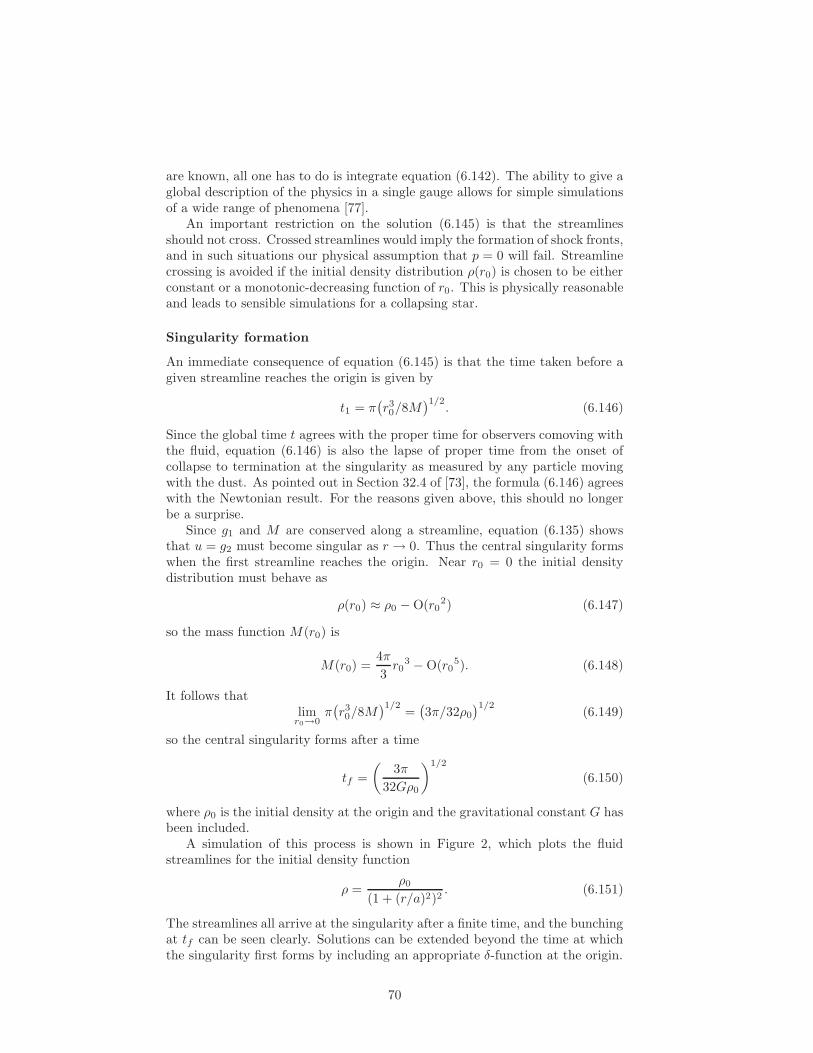
are known, all one has to do is integrate equation (6.142). The ability to give aglobal description of the physics in a single gauge allows for simple simulationsof a wide range of phenomena [77].

An important restriction on the solution (6.145) is that the streamlinesshould not cross. Crossed streamlines would imply the formation of shock fronts,and in such situations our physical assumption that p = 0 will fail. Streamlinecrossing is avoided if the initial density distribution ρ(r0) is chosen to be eitherconstant or a monotonic-decreasing function of r0. This is physically reasonableand leads to sensible simulations for a collapsing star.

Singularity formation

An immediate consequence of equation (6.145) is that the time taken before agiven streamline reaches the origin is given by

t1 = π(

r30/8M)1/2

. (6.146)

Since the global time t agrees with the proper time for observers comoving withthe fluid, equation (6.146) is also the lapse of proper time from the onset ofcollapse to termination at the singularity as measured by any particle movingwith the dust. As pointed out in Section 32.4 of [73], the formula (6.146) agreeswith the Newtonian result. For the reasons given above, this should no longerbe a surprise.

Since g1 and M are conserved along a streamline, equation (6.135) showsthat u = g2 must become singular as r → 0. Thus the central singularity formswhen the first streamline reaches the origin. Near r0 = 0 the initial densitydistribution must behave as

ρ(r0) ≈ ρ0 − O(r02) (6.147)

so the mass function M(r0) is

M(r0) =4π

3r0

3 − O(r05). (6.148)

It follows thatlimr0→0

π(

r30/8M)1/2

=(

3π/32ρ0

)1/2(6.149)

so the central singularity forms after a time

tf =

(

3π

32Gρ0

)1/2

(6.150)

where ρ0 is the initial density at the origin and the gravitational constant G hasbeen included.

A simulation of this process is shown in Figure 2, which plots the fluidstreamlines for the initial density function

ρ =ρ0

(1 + (r/a)2)2. (6.151)

The streamlines all arrive at the singularity after a finite time, and the bunchingat tf can be seen clearly. Solutions can be extended beyond the time at whichthe singularity first forms by including an appropriate δ-function at the origin.

70

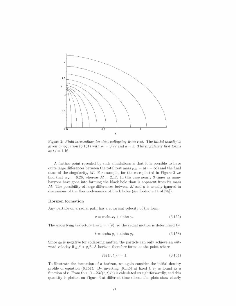
0

0.5

1

1.5

2

0 0.5 1

r

t

Figure 2: Fluid streamlines for dust collapsing from rest. The initial density isgiven by equation (6.151) with ρ0 = 0.22 and a = 1. The singularity first formsat tf = 1.16.

A further point revealed by such simulations is that it is possible to havequite large differences between the total rest mass µ∞ = µ(r = ∞) and the finalmass of the singularity, M . For example, for the case plotted in Figure 2 wefind that µ∞ = 6.26, whereas M = 2.17. In this case nearly 3 times as manybaryons have gone into forming the black hole than is apparent from its massM . The possibility of large differences between M and µ is usually ignored indiscussions of the thermodynamics of black holes (see footnote 14 of [78]).

Horizon formation

Any particle on a radial path has a covariant velocity of the form

v = coshu et + sinhu er. (6.152)

The underlying trajectory has x = h(v), so the radial motion is determined by

r = coshu g2 + sinhu g1. (6.153)

Since g2 is negative for collapsing matter, the particle can only achieve an out-ward velocity if g1

2 > g22. A horizon therefore forms at the point where

2M(r, t)/r = 1. (6.154)

To illustrate the formation of a horizon, we again consider the initial densityprofile of equation (6.151). By inverting (6.145) at fixed t, r0 is found as afunction of r. From this, (1−2M(r, t)/r) is calculated straightforwardly, and thisquantity is plotted on Figure 3 at different time slices. The plots show clearly

71

1−

2M/r

x

Figure 3: Simulation of collapsing dust in the Newtonian gauge. Successive timeslices for the horizon function (1− 2M(r, t)/r) versus x are shown, with the topcurve corresponding to t = 0 and lower curves to successively later times. Theinitial velocity is zero, and the initial density profile is given by equation (6.151)with ρ0 = 0.22 and a = 1. There is no horizon present initially, but a trappedregion quickly forms, since in regions where 1 − 2M/r < 0 photons can onlymove inwards.

that the horizon forms at a finite distance from the origin. It is conventional toextend the horizon back in time along the past light-cone to the origin (r = 0),since any particle inside this surface could not have reached the point at which1 − 2M/r first drops to zero, and hence is also trapped [79]. The ease withwhich horizon formation is treated again illustrates the advantages of workingin a non-diagonal gauge. Such considerations will clearly be important whenperforming numerical studies of more realistic collapse scenarios.

A final point is that, since u is negative, it follows that f1g2−f2g1 = u mustalso be negative. This tells us that the fields that remain after the collapseprocess has finished are in the class defined by f1g2 − f2g1 = −1 at the horizon.This time direction is then frozen into the fields, as discussed in Section 6.4.

6.6 Cosmology

The equations of Table 4 are sufficiently general to deal with cosmology as wellas astrophysics. In recent years, however, it has once more become fashionableto include a cosmological constant in the field equations. The derivation ofSection 6.2 is largely unaffected by the inclusion of the cosmological term, andonly a few modifications to Table 4 are required. The full set of equations with

72

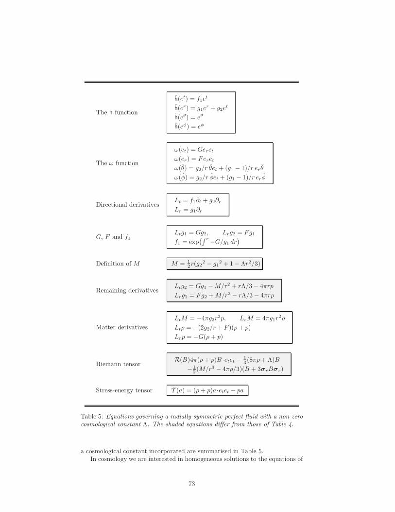
The h-function

h(et) = f1et

h(er) = g1er + g2e

t

h(eθ) = eθ

h(eφ) = eφ

The ω function

ω(et) = Geret

ω(er) = Feret

ω(θ) = g2/r θet + (g1 − 1)/r erθ

ω(φ) = g2/r φet + (g1 − 1)/r erφ

Directional derivativesLt = f1∂t + g2∂r

Lr = g1∂r

G, F and f1Ltg1 = Gg2, Lrg2 = Fg1

f1 = exp(∫ r −G/g1 dr

)

Definition of M M = 12r(g2

2 − g12 + 1 − Λr2/3)

Remaining derivativesLtg2 = Gg1 −M/r2 + rΛ/3 − 4πrp

Lrg1 = Fg2 +M/r2 − rΛ/3 − 4πrρ

Matter derivatives

LtM = −4πg2r2p, LrM = 4πg1r

2ρ

Ltρ = −(2g2/r + F )(ρ+ p)

Lrp = −G(ρ+ p)

Riemann tensorR(B)4π(ρ + p)B ·etet − 1

3 (8πρ+ Λ)B

− 12 (M/r3 − 4πρ/3)(B + 3σrBσr)

Stress-energy tensor T (a) = (ρ+ p)a·etet − pa

Table 5: Equations governing a radially-symmetric perfect fluid with a non-zerocosmological constant Λ. The shaded equations differ from those of Table 4.

a cosmological constant incorporated are summarised in Table 5.In cosmology we are interested in homogeneous solutions to the equations of

73

Table 5. Such solutions are found by setting ρ and p to functions of t only, andit follows immediately from the Lrp equation that

G = 0, and f1 = 1. (6.155)

For homogeneous fields the Weyl component of the Riemann tensor must vanish,since this contains directional information through the er vector. The vanishingof this term requires that

M(r, t) =4

3πr3ρ, (6.156)

which is consistent with the LrM equation. The LtM and Ltρ equations nowreduce to

F = g2/r (6.157)

andρ = −3g2(ρ+ p)/r. (6.158)

But we know that Lrg2 = Fg1, which can only be consistent with (6.157) if

F = H(t), g2(r, t) = rH(t). (6.159)

The Ltg2 equation now reduces to a simple equation for H ,

H +H2 − Λ/3 = −4π

3(ρ+ 3p). (6.160)

Finally, we are left with the following pair of equations for g1:

Ltg1 = 0 (6.161)

Lrg1 = (g12 − 1)/r. (6.162)

The latter equation yields g12 = 1 + r2φ(t) and the former reduces to

φ = −2H(t)φ. (6.163)

Hence g1 is given by

g12 = 1 − kr2 exp

(

−2

∫ t

H(t′) dt′)

, (6.164)

where k is an arbitrary constant of integration. It is straightforward to checkthat (6.164) is consistent with the equations for H and ρ. The full set of equa-tions describing a homogeneous perfect fluid are summarised in Table 6.

At first sight, the equations of Table 6 do not resemble the usual Friedmannequations. The Friedmann equations are recovered straightforwardly, however,by setting

H(t) =S(t)

S(t). (6.165)

With this substitution we find that

g12 = 1 − kr2/S2 (6.166)

74

The h-functionh(a) = a+ a·er

(

(g1 − 1)er +H(t)ret)

g12 = 1 − kr2 exp

(

−2∫ tH(t′) dt′

)

The ω function ω(a) = H(t)a∧et − (g1 − 1)/r a∧(eret)et

The density 8πρ/3 = H(t)2 − Λ/3 + k exp(

−2∫ tH(t′) dt′

)

Dynamical

equations

H +H2 − Λ/3 = −4π/3 (ρ+ 3p)

ρ = −3H(t)(ρ+ p)

Table 6: Equations governing a homogeneous perfect fluid.

and that the H and density equations become

S

S− Λ

3= −4π

3(ρ+ 3p) (6.167)

and

S2 + k

S2− Λ

3=

8π

3ρ, (6.168)

recovering the Friedmann equations in their standard form [80]. The intrinsictreatment has therefore led us to work directly with the ‘Hubble velocity’ H(t),rather than the ‘distance’ scale S(t). There is a good reason for this. Once theWeyl tensor is set to zero, the Riemann tensor reduces to

R(B) = 4π(ρ+ p)B ·etet − 13 (8πρ+ Λ)B, (6.169)

and we have now lost contact with an intrinsically-defined distance scale. Wecan therefore rescale the radius variable r with an arbitrary function of t (or r)without altering the Riemann tensor. The Hubble velocity, on the other hand,is intrinsic and it is therefore not surprising that our treatment has led directlyto equations for this.

Among the class of radial rescalings a particularly useful one is to rescale rto r′ = S(t)r. This is achieved with the transformation

f(x) = x·et et + Sx∧et et, (6.170)

so that, on applying equation (3.9), the transformed h-function is

h′(a) = a·et et +

1

S

(

(1 − kr2)1/2a·er er + a∧σr σr)

. (6.171)

The function (6.171) reproduces the standard line element used in cosmology.We can therefore use the transformation (6.170) to move between the ‘Newto-nian’ gauge developed here and the gauge of (6.171). This is useful for later

75

sections, where the Maxwell and Dirac equations are solved in a cosmologicalbackground described by (6.171). The differences between these gauges canbe understood by considering geodesic motion. A particle at rest with respectto the cosmological frame (defined by the cosmic microwave background) hasv = et. In the gauge of (6.171) such a particle is not moving in the flatspacebackground (the distance variable r is equated with the comoving coordinate).In the Newtonian gauge, on the other hand, comoving particles are moving out-wards radially at a velocity r = H(t)r, though this expansion centre is not anintrinsic feature. Of course, attempting to distinguish these pictures is a point-less exercise, since all observables must be gauge-invariant. All that is of physicalrelevance is that, if two particles are at rest with respect to the cosmologicalframe (defined by the cosmic microwave background), then the light-travel timebetween these particles is an increasing function of time and light is redshiftedas it travels between them.

Dust models

The utility of the Newtonian gauge in cosmology has been independently dis-covered by other authors [62, 81]. Here we illustrate its advantages for dustmodels (p = 0). Setting p to zero implies that

H(t) = −ρ/3ρ, (6.172)

sog1

2 = 1 − kr2ρ2/3 (6.173)

and

H(t) =

(

8π

3ρ− kρ2/3 +

Λ

3

)1/2

. (6.174)

We are therefore left with a single first-order differential equation for ρ. Explicitsolutions of this equations are often not needed, as we can usually parameterisetime by the density ρ(t).

If we now look at the trajectories defined by the fluid, these have v = etwhich implies that

x = et + rH(t)er. (6.175)

It follows thatr/r = H(t) = −ρ/3ρ (6.176)

and hence thatr/r0 = (ρ/ρ0)

−1/3. (6.177)

The fluid streamlines form a family of spacetime curves spreading out from theorigin at the initial singularity (when ρ = ∞). The Newtonian gauge thereforedescribes an expanding universe in a very simple, almost naive manner. Since allpoints in a homogeneous cosmology are equivalent, we can consider ourselves tobe located at r = 0. The Newtonian gauge then pictures our observable universeas a ball of dust expanding outwards radially from us.

While the picture provided by the Newtonian gauge has no physical realityof its own, it does have some heuristic merit and can provide a useful aid toone’s physical intuition. For example, consider the familiar relationship betweenangular size and redshift. An initially surprising feature of this relationship is

76

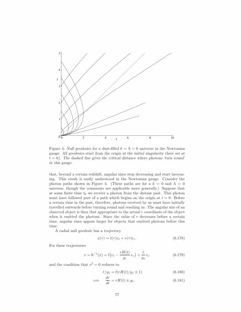
0

1

2

3

4

5

0 2 4 6 8 10r

t

Figure 4: Null geodesics for a dust-filled k = Λ = 0 universe in the Newtoniangauge. All geodesics start from the origin at the initial singularity (here set att = 0). The dashed line gives the critical distance where photons ‘turn round’in this gauge.

that, beyond a certain redshift, angular sizes stop decreasing and start increas-ing. This result is easily understood in the Newtonian gauge. Consider thephoton paths shown in Figure 4. (These paths are for a k = 0 and Λ = 0universe, though the comments are applicable more generally.) Suppose thatat some finite time t0 we receive a photon from the distant past. This photonmust have followed part of a path which begins on the origin at t = 0. Beforea certain time in the past, therefore, photons received by us must have initiallytravelled outwards before turning round and reaching us. The angular size of anobserved object is then that appropriate to the actual r coordinate of the objectwhen it emitted the photons. Since the value of r decreases before a certaintime, angular sizes appear larger for objects that emitted photons before thistime.

A radial null geodesic has a trajectory

x(τ) = t(τ)et + r(τ)er . (6.178)

For these trajectories

v = h−1(x) = t

(

et −rH(t)

g1er)

+r

g1er (6.179)

and the condition that v2 = 0 reduces to

r/g1 = t(rH(t)/g1 ± 1) (6.180)

=⇒ dr

dt= rH(t) ± g1. (6.181)

77

Since H(t) is positive in a cooling universe, the distance at which photons ‘turnround’ is defined by

rc =g1H(t)

=

(

8πρ

3+

Λ

3

)−1/2

. (6.182)

(In [59] we mistakenly referred to this distance as a particle horizon.) Fork = Λ = 0 it is simple to show that this distance corresponds to a redshift of1.25. This result relates physically measurable quantities, so is gauge invariant.

Closed universe models

The Newtonian gauge presents a particularly simple picture for a closed universe(k > 0). For k > 0 the requirement that 1 − kr2ρ2/3 is positive means that

r3ρ > k−3/2. (6.183)

This places a limit on the speed with which the dust can expand, so the solutiondescribes a finite ball of dust expanding into a vacuum. This ball expands outto some fixed radius before turning round and contracting back to the origin.The turning point is achieved where H(t) = 0 so, for Λ = 0, this occurs when

ρ = (3k/8π)3. (6.184)

The maximum radius is therefore

rmax =8π

3k3/2. (6.185)

The time taken to reach the future singularity is given by (6.150), since thiscosmological model is a special case of spherical collapse in which the densityis uniform. This picture of a model for a closed universe is both simple andappealing. It allows us to apply Newtonian reasoning while ensuring consistencywith the full relativistic theory.

The finite ball model for a k > 0 cosmology is clearly useful when consideringexperiments with particles carried out near the origin, but globally one mustconsider the boundary properties of the ball. A crucial question is whether theparticle horizon (the largest region of the universe with which an observer atthe origin is in causal contact) extends past the edge of the ball or not. It canbe shown that this horizon always lies inside the radius at which g1 becomesimaginary, except at the turnaround point (the point at which the ball reachesits maximum radius), where the two radii coincide. A suitable choice of cutoffradius is therefore available in either the expanding or contracting phase sep-arately, but what happens at the turnaround point is potentially ambiguous.When discussing field theory, however, the finite ball model is inadequate. Onemust instead use a global gauge so, in Section 7.4, we introduce the ‘stereo-graphic projection gauge’. This provides a global solution which can be shownto be spatially closed. This solution is used in the study of electromagnetism(Section 7.4) and the Dirac equation (Section 8.3) in a cosmological background.It is possible to treat the stereographic projection gauge solution in a form ofthe Newtonian gauge, though this possibility is not explored here.

78

7 Electromagnetism in a gravitational

background

In Section 4 we derived field equations for the gravitational and Dirac fields.We now turn to the derivation of the Maxwell equations in a gravitationalbackground. A number of applications of these equations are then discussed,including a simple derivation of the characteristic surfaces for both the Maxwelland Dirac equations.

The basic dynamical variable is the electromagnetic vector potential A, forwhich the coupling to spinor fields was derived in Section 3.3. Under phaserotations of the spinor field, A transforms as

eA 7→ eA−∇φ. (7.1)

It follows that, under a displacement, A must transform in the same way as ∇φ,that is,

A(x) 7→ f(A(x′)). (7.2)

The covariant form of the vector potential is therefore

A = h(A), (7.3)

which is the term that appeared in the Dirac equation (3.63).From A, the Faraday bivector F is defined by

F = ∇∧A. (7.4)

This definition implies that, under displacements, F (x) is transformed to F ′(x),where

F ′(x) = ∇∧ fA(x′)

= f(∇x′∧A(x′))

= fF (x′). (7.5)

It follows that the covariant analogue of F is defined by

F = h(F ), (7.6)

which is covariant under position and rotation-gauge transformations, and isinvariant under phase changes.

The same covariant quantity F is obtained if one follows the route used forthe construction of R(a ∧ b) at (4.2). In particular, the contracted commutatorof two covariant derivatives gives (in the absence of torsion)

h(eν)∧h(eµ)[Dµ, Dν ]ψ = 12 h(∂b)h(∂a)R(a∧b)ψ

= 12Rψ. (7.7)

The analogous construction for the ‘internal’ covariant derivative

DIaψ = a·∇ψ − ea·AψIσ3 (7.8)

79

gives

h(eν)∧h(eµ)[DIµ, D

Iν ]ψ = eh(∂b)∧h(∂a)(a∧b)·FψIσ3

= 2eFψIσ3, (7.9)

which clearly identifies F as a covariant quantity. Unlike R, however, F is abivector and equation (7.9) exhibits a curious interaction between this bivectoron the left of ψ, and the fixed bivector Iσ3 on the right.

Having defined the covariant bivector F , it is clear that the appropriategeneralisation of the electromagnetic action to include gravitational interactionsis

S =

∫

|d4x| det(h)−1 (12F ·F −A·J ), (7.10)

where here J is the covariant charge current. Unlike the Dirac action, therotation-gauge field Ω(a) does not appear in this action. It follows that theelectromagnetic field does not act as a source of spin. The action (7.10) isvaried with respect to A, with h(a) and J treated as external fields. The resultof this is the equation

∇·G = J, (7.11)

where

G = h h(F ) det(h)−1 (7.12)

and

J = h(J ) det(h)−1. (7.13)

Equation (7.11) combines with the identity

∇∧F = 0 (7.14)

to form the full set of Maxwell equations in a gravitational background. Weagain see that the classical field equations can be expressed in a form fromwhich all reference to the rotation gauge has been removed.

Some insight into the equations (7.11) and (7.14) is obtained by performinga space-time split (see Section 2.1) and writing

F = E + IB (7.15)

G = D + IH (7.16)

Jγ0 = ρ+ J . (7.17)

In terms of these variables Maxwell’s equations in a gravitational backgroundtake the familiar form

∇·B = 0 ∇·D = ρ

∇×E = −∂B

∂t∇×H = J +

∂D

∂t

(7.18)

where ∇ = γ0 ∧∇ = σi∂xi is the 3D vector derivative, and the bold cross × isthe traditional vector cross product:

a×b = −I a×b. (7.19)

80

Equation (7.18) shows that the h-field defines the dielectric properties of thespace through which the electromagnetic fields propagate, with det(h)−1

h h de-termining the generalized permittivity/permeability tensor. Many phenomena,including the bending of light, can be understood easily in terms of the proper-ties of the dielectric defined by the h-field.

Covariant form of the Maxwell equations

So far we have failed to achieve a manifestly covariant form of the Maxwellequations. We have, furthermore, failed to unite the separate equations into asingle equation. In the absence of gravitational effects the equations ∇·F = Jand ∇∧F = 0 combine into the single equation

∇F = J. (7.20)

The significance of this equation is that the ∇ operator is invertible, whereasthe separate ∇· and ∇∧ operators are not [11, 26]. Clearly, we expect thatsuch a unification should remain possible after the gravitational gauge fieldshave been introduced. To find a covariant equation, we first extend the ‘wedge’equation (4.37) to include higher-grade terms. To make the derivation generalwe include the spin term, in which case we find that

D∧ ˙h(a∧b) = (D∧ ˙

h(a))∧h(b) − h(a)∧(D∧ ˙h(b))

= κ(h(a)·S)∧h(b) − κh(a)∧(h(b)·S)

= κS×h(a∧b) (7.21)

and, more generally, we can write

D∧h(Ar) = h(∇∧Ar) + κ〈Sh(Ar)〉r+1. (7.22)

We can therefore replace equation (7.14) by

D∧F − κS×F = 0. (7.23)

We next use the rearrangement

∇·(h(F) det(h)−1) = I∇∧(Ih(F) det(h)−1)

= I∇∧(h−1(IF))

= I h−1(

D∧(IF) + κ(IF)×S)

(7.24)

to write equation (7.11) as

D·F − κS·F = I h(JI) = J . (7.25)

Equations (7.23) and (7.25) now combine into the single equation

DF − κSF = J , (7.26)

which achieves our objective. Equation (7.26) is manifestly covariant and theappearance of the DF term is precisely what one might expect on ‘minimal-coupling’ grounds. The appearance of the spin term is a surprise, however.Gauge arguments alone would not have discovered this term and it is only

81

through the construction of a gauge-invariant action integral that the term isfound. Equation (7.26) should be particularly useful when considering electro-magnetic effects in regions of high spin density, such as neutron stars.

To complete the description of electromagnetism in a gravitational back-ground we need a formula for the free-field stress-energy tensor. Applying thedefinition (4.20) we construct

Tem(h−1(a)) = 12 det(h) ∂h(a)

⟨

h(F )h(F ) det(h)−1⟩

= h(a·F )·F − 12h

−1(a)F ·F . (7.27)

Hence,

Tem(a) = h(h(a)·F )·F − 12aF ·F

= (a·F)·F − 12aF ·F

= − 12FaF , (7.28)

which is the natural covariant extension of the gravitation-free form −FaF/2.The tensor (7.28) is symmetric, as one expects for fields with vanishing spindensity.

7.1 Characteristic surfaces

In their spacetime algebra form the Maxwell and Dirac equations are both first-order differential equations involving the vector derivative ∇. For electromag-netism, this first-order form of the equations offers many advantages over theequivalent second-order theory [14, 26]. We have now seen that gravitational in-teractions modify both these equations in such a way that the vector derivative∇ is replaced by the position-gauge covariant derivative h(∇). As an illustrationof the utility of first-order equations, both without and with gravitational effects,we now give a simple derivation of the properties of characteristic surfaces.

Consider, initially, a generic equation of the type

∇ψ = f(ψ, x) (7.29)

where ψ is some arbitrary field, and f is some known function. Suppose that aninitial set of data is given over some three-dimensional surface in spacetime, andwe wish to propagate this information off the surface into the adjoining region.We pick three vectors, a, b and c, which are tangent to the surface. From ourinitial data we can construct a·∇ψ, b·∇ψ and c·∇ψ. Now define

n = I a∧b∧c (7.30)

and use n∇ = n·∇+ n∧∇ to decompose (7.29) into

n·∇ψ = −n∧∇ψ + nf(ψ). (7.31)

The right-hand side of (7.31) contains the term

n∧∇ψ = I(a∧b∧c)·∇ψ= I(a∧b c·∇ψ − a∧c b·∇ψ+ b∧c a·∇ψ), (7.32)

82

which is therefore known. It follows that we know all the terms on the right-hand side of equation (7.31) and can therefore construct n·∇ψ. This gives us thederivative required to propagate off the surface. The only situation for whichpropagation is impossible is when n remains in the surface. This occurs when

n∧(a∧b∧c) = 0

=⇒ n∧(nI) = 0

=⇒ n·n = 0. (7.33)

It follows that the characteristic surfaces for any first-order equation of the typedefined by (7.29) are null surfaces. These considerations automatically includethe Maxwell and Dirac equations. It is notable how this result follows frompurely algebraic considerations.

The generalisation to a gravitational background is straightforward. Equa-tion (7.26) is generalised to

h(∇)ψ = f(ψ), (7.34)

and we assume that a gauge choice has been made so that all the fields (apartfrom ψ) are known functions of x. Again, we assume that the initial data consistof values for ψ over some three-dimensional surface, so we can still determinea·∇ψ etc. Since

a·∇ = h−1(a)·h(∇) (7.35)

it follows that the vector of interest is now

Ih−1(a)∧h−1(b)∧h

−1(c) = Ih−1(nI) = h(n) det(h)−1. (7.36)

This time we multiply equation (7.34) by h(n) and find that h(n) · h(∇)ψ canbe constructed entirely from known quantities. We can therefore propagate inthe h h(n) direction, so we now require that this vector does not lie in the initialsurface. The analogue of (7.33) is therefore

h h(n)·n = 0, or h(n)2 = 0, (7.37)

and the characteristic surfaces are now those for which h(n) is null. This is theobvious covariant extension of n being a null vector.

7.2 Point charge in a black-hole background

The problem of interest here is to find the fields generated by a point source heldat rest outside the horizon of a radially-symmetric black hole. The h-function inthis case can be taken as that of equation (6.79). The solution to this problemcan be found by adapting the work of Copson [82] and Linet [83] to the presentgauge choices. Assuming, for simplicity, that the charge is placed on the z-axisa distance a from the origin (a > 2M), the vector potential can be written interms of a single scalar potential V (r, θ) as

A = V (r, θ)

(

et +

√2Mr

r − 2Mer

)

. (7.38)

83

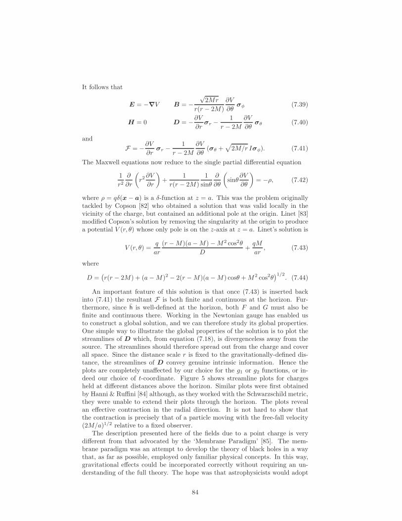
It follows that

E = −∇V B = −√

2Mr

r(r − 2M)

∂V

∂θσφ (7.39)

H = 0 D = −∂V∂r

σr −1

r − 2M

∂V

∂θσθ (7.40)

and

F = −∂V∂r

σr −1

r − 2M

∂V

∂θ(σθ +

√

2M/r Iσφ). (7.41)

The Maxwell equations now reduce to the single partial differential equation

1

r2∂

∂r

(

r2∂V

∂r

)

+1

r(r − 2M)

1

sinθ

∂

∂θ

(

sinθ∂V

∂θ

)

= −ρ, (7.42)

where ρ = qδ(x − a) is a δ-function at z = a. This was the problem originallytackled by Copson [82] who obtained a solution that was valid locally in thevicinity of the charge, but contained an additional pole at the origin. Linet [83]modified Copson’s solution by removing the singularity at the origin to producea potential V (r, θ) whose only pole is on the z-axis at z = a. Linet’s solution is

V (r, θ) =q

ar

(r −M)(a−M) −M2 cos2θ

D+qM

ar, (7.43)

where

D =(

r(r − 2M) + (a−M)2 − 2(r −M)(a−M) cosθ +M2 cos2θ)1/2

. (7.44)

An important feature of this solution is that once (7.43) is inserted backinto (7.41) the resultant F is both finite and continuous at the horizon. Fur-thermore, since h is well-defined at the horizon, both F and G must also befinite and continuous there. Working in the Newtonian gauge has enabled usto construct a global solution, and we can therefore study its global properties.One simple way to illustrate the global properties of the solution is to plot thestreamlines of D which, from equation (7.18), is divergenceless away from thesource. The streamlines should therefore spread out from the charge and coverall space. Since the distance scale r is fixed to the gravitationally-defined dis-tance, the streamlines of D convey genuine intrinsic information. Hence theplots are completely unaffected by our choice for the g1 or g2 functions, or in-deed our choice of t-coordinate. Figure 5 shows streamline plots for chargesheld at different distances above the horizon. Similar plots were first obtainedby Hanni & Ruffini [84] although, as they worked with the Schwarzschild metric,they were unable to extend their plots through the horizon. The plots revealan effective contraction in the radial direction. It is not hard to show thatthe contraction is precisely that of a particle moving with the free-fall velocity(2M/a)1/2 relative to a fixed observer.

The description presented here of the fields due to a point charge is verydifferent from that advocated by the ‘Membrane Paradigm’ [85]. The mem-brane paradigm was an attempt to develop the theory of black holes in a waythat, as far as possible, employed only familiar physical concepts. In this way,gravitational effects could be incorporated correctly without requiring an un-derstanding of the full theory. The hope was that astrophysicists would adopt

84

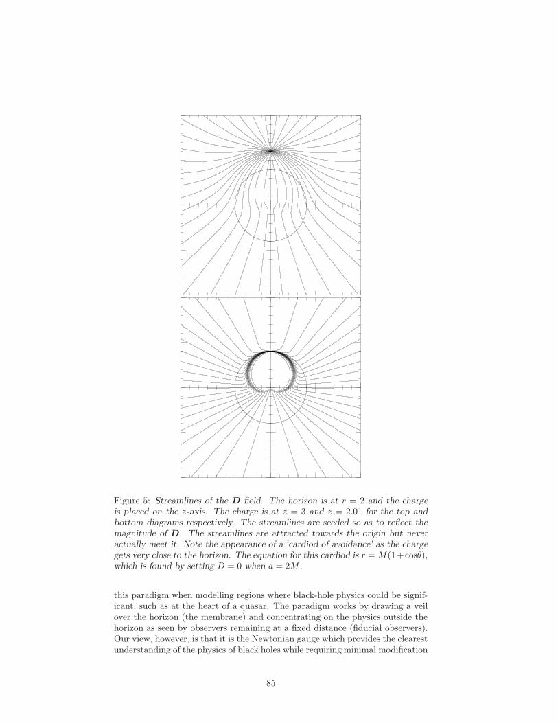
Figure 5: Streamlines of the D field. The horizon is at r = 2 and the chargeis placed on the z-axis. The charge is at z = 3 and z = 2.01 for the top andbottom diagrams respectively. The streamlines are seeded so as to reflect themagnitude of D. The streamlines are attracted towards the origin but neveractually meet it. Note the appearance of a ‘cardiod of avoidance’ as the chargegets very close to the horizon. The equation for this cardiod is r = M(1+cosθ),which is found by setting D = 0 when a = 2M .

this paradigm when modelling regions where black-hole physics could be signif-icant, such as at the heart of a quasar. The paradigm works by drawing a veilover the horizon (the membrane) and concentrating on the physics outside thehorizon as seen by observers remaining at a fixed distance (fiducial observers).Our view, however, is that it is the Newtonian gauge which provides the clearestunderstanding of the physics of black holes while requiring minimal modification

85

to Newtonian and special-relativistic ideas. Furthermore, writing the Maxwellequations in the form (7.18) removes any difficulties in applying conventionalreasoning to the study electromagnetism in a gravitational background.

There are other ways that our approach offers advantages over the mem-brane paradigm. When applying the membrane paradigm one has to work withquantities which are singular at the horizon, and this is hardly a recipe for ap-plying traditional intuition! As we have seen, once formulated in the Newtoniangauge (or any other gauge admissible in GTG) all physical quantities are finite.The membrane paradigm also warns physicists against producing plots such asFigure 5, because such plots depend on the choice of radial coordinate. Butour intrinsic approach makes it clear that such plots are meaningful, becauser is determined uniquely by the Riemann tensor. Presenting the plots in theform of Figure 5 enables direct physical information to be read off. In short,the simple physical picture provided by our intrinsic method and Newtonian-gauge solution disposes of any need to adopt the artificial ideas advocated bythe membrane paradigm.

7.3 Polarisation repulsion

An interesting feature of the above solution (7.43) is the existence of a repulsive‘polarisation’ force [86], one effect of which is that a smaller force is neededto keep a charged particle at rest outside a black hole than an uncharged one.In their derivation of this force, Smith & Will [86] employed a complicatedenergy argument that involved renormalising various divergent integrals. Herewe show that the same force can be derived from a simple argument based on thepolarisation effects of the dielectric described by a black hole. First, however,we must be clear how force is defined. In the presence of an electromagneticfield the equation of motion for a point particle (4.63) is modified to

mv = (qF −mω(v))·v. (7.45)

We therefore expect that any additional force should also be described by acovariant bivector which couples to the velocity the same way that F does. So,if we denote the externally applied force as W , the equation of motion for aneutral test particle becomes

mv = (W −mω(v))·v. (7.46)

Now, suppose that W is chosen so that the particle remains at a fixed distancea outside the horizon of a black hole. The equation for the trajectory is

x(τ) = t(τ)et + aer(θ0, φ0), (7.47)

where the constants θ0 and φ0 specify the angular position of the particle. Thecovariant velocity is

v = th−1(et), (7.48)

and the condition that v2 = 1 forces

t2(1 − 2M/a) = 1, (7.49)

86

so that t, and hence v, are constant. Equation (7.46) now reduces to

W −mω(v) = 0 (7.50)

=⇒ W = mtΩ(et) =Mm

a2

(

1 − 2M

a

)−1/2

σa, (7.51)

where σa is the unit outward spatial vector from the source to the particle. Themagnitude of the force is therefore

|W | =Mm

a2

(

1 − 2M

a

)−1/2

(7.52)

and it is not hard to check that this result is gauge-invariant. Equation (7.52)reduces to the Newtonian formula at large distances and becomes singular asthe horizon is approached, where an infinite force is required to remain at rest.

We now want to see how this expression for the force is modified if the particleis charged and feels a force due to its own polarisation field. From (7.45) theextra term in the force is simply F , and only the radial term contributes. Fromequation (7.41) this is just −∂rV σr. Since the charge lies on the z axis, weneed only look at V along this axis, for which

V (z) =q

|z − a| −qM

|z − a|

(

1

a+

1

z

)

+qM

az. (7.53)

The singular terms must be due to the particle’s own Coulomb field, and sodo not generate a polarisation force. The only term that generates a force istherefore the final one, which is precisely the term that Linet added to Copson’soriginal formula! This term produces an outward-directed force on the charge,of magnitude q2M/a3. The applied force is therefore now

W =

(

Mm

a2

(

1 − 2M

a

)−1/2

− Mq2

a3

)

σa, (7.54)

so a smaller force is needed to keep the particle at rest outside the horizon. Thisresult agrees with that found in [86], though our derivation avoids the need forinfinite mass renormalisation and is considerably simpler. This result is a goodexample of the importance of finding global solutions. The polarisation force isfelt outside the horizon, yet the correction term that led to it was motivated bythe properties of the field at the origin.

7.4 Point charge in a k > 0 cosmology

We saw in Section 6.6 that one form of the h-function for a homogeneous cos-mology is defined by (6.171)

h(a) = a·et et + α(

(1 − kr2)1/2a·er er + a∧σr σr)

, (7.55)

where α = 1/S. When k is positive, however, the function (7.55) is undefinedfor r > k−1/2 and so fails to define a global solution. A globally-valid solutionis obtained with the displacement

f(x) = x·et et +r

1 + kr2/4er, (7.56)

87

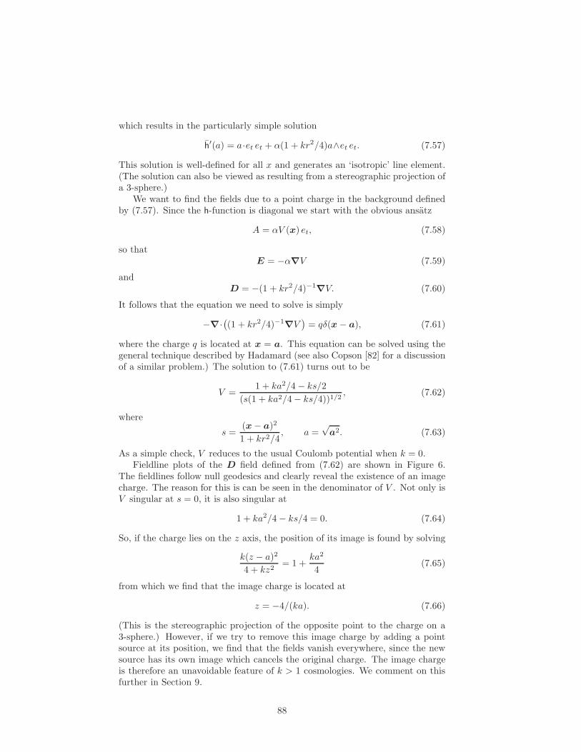
which results in the particularly simple solution

h′(a) = a·et et + α(1 + kr2/4)a∧et et. (7.57)

This solution is well-defined for all x and generates an ‘isotropic’ line element.(The solution can also be viewed as resulting from a stereographic projection ofa 3-sphere.)

We want to find the fields due to a point charge in the background definedby (7.57). Since the h-function is diagonal we start with the obvious ansatz

A = αV (x) et, (7.58)

so thatE = −α∇V (7.59)

andD = −(1 + kr2/4)−1∇V. (7.60)

It follows that the equation we need to solve is simply

−∇·(

(1 + kr2/4)−1∇V)

= qδ(x − a), (7.61)

where the charge q is located at x = a. This equation can be solved using thegeneral technique described by Hadamard (see also Copson [82] for a discussionof a similar problem.) The solution to (7.61) turns out to be

V =1 + ka2/4 − ks/2

(s(1 + ka2/4 − ks/4))1/2, (7.62)

where

s =(x − a)2

1 + kr2/4, a =

√a2. (7.63)

As a simple check, V reduces to the usual Coulomb potential when k = 0.Fieldline plots of the D field defined from (7.62) are shown in Figure 6.

The fieldlines follow null geodesics and clearly reveal the existence of an imagecharge. The reason for this is can be seen in the denominator of V . Not only isV singular at s = 0, it is also singular at

1 + ka2/4 − ks/4 = 0. (7.64)

So, if the charge lies on the z axis, the position of its image is found by solving

k(z − a)2

4 + kz2= 1 +

ka2

4(7.65)

from which we find that the image charge is located at

z = −4/(ka). (7.66)

(This is the stereographic projection of the opposite point to the charge on a3-sphere.) However, if we try to remove this image charge by adding a pointsource at its position, we find that the fields vanish everywhere, since the newsource has its own image which cancels the original charge. The image chargeis therefore an unavoidable feature of k > 1 cosmologies. We comment on thisfurther in Section 9.

88

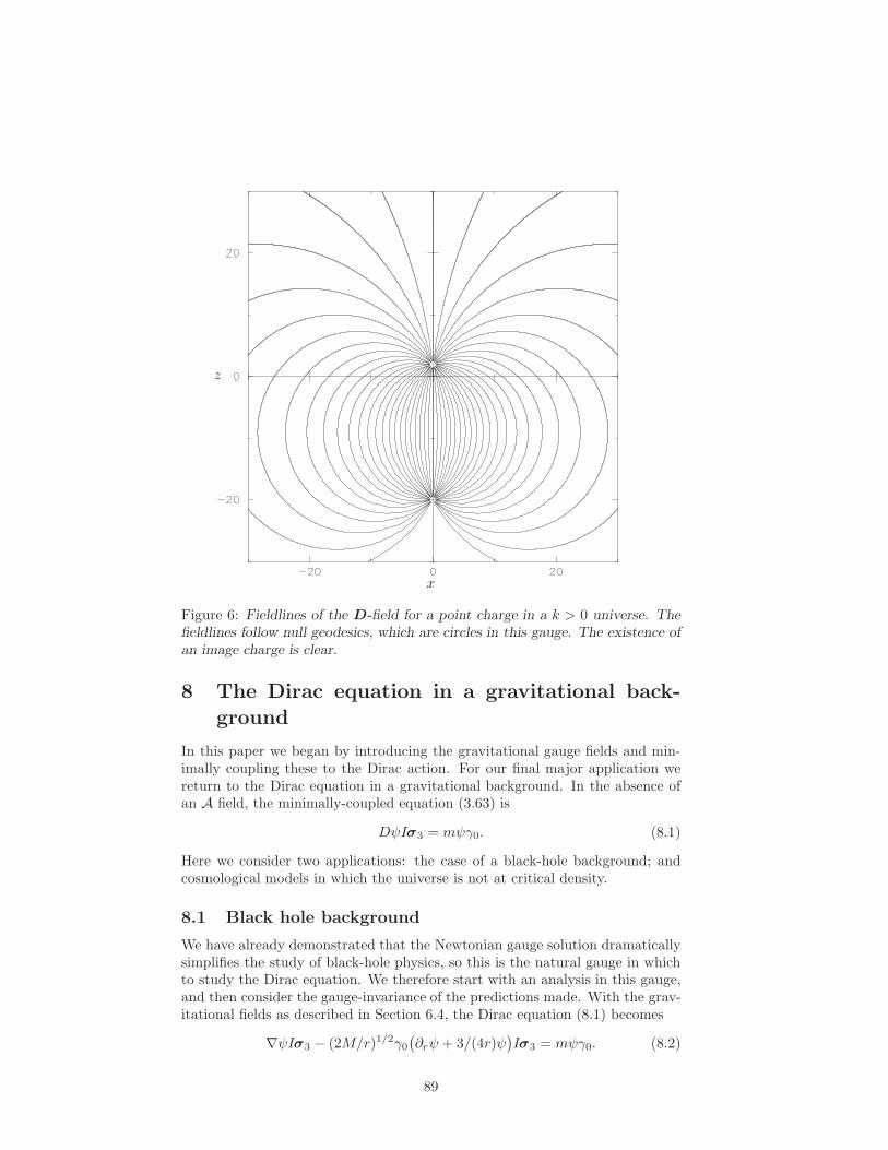
x

z

Figure 6: Fieldlines of the D-field for a point charge in a k > 0 universe. Thefieldlines follow null geodesics, which are circles in this gauge. The existence ofan image charge is clear.

8 The Dirac equation in a gravitational back-

ground

In this paper we began by introducing the gravitational gauge fields and min-imally coupling these to the Dirac action. For our final major application wereturn to the Dirac equation in a gravitational background. In the absence ofan A field, the minimally-coupled equation (3.63) is

DψIσ3 = mψγ0. (8.1)

Here we consider two applications: the case of a black-hole background; andcosmological models in which the universe is not at critical density.

8.1 Black hole background

We have already demonstrated that the Newtonian gauge solution dramaticallysimplifies the study of black-hole physics, so this is the natural gauge in whichto study the Dirac equation. We therefore start with an analysis in this gauge,and then consider the gauge-invariance of the predictions made. With the grav-itational fields as described in Section 6.4, the Dirac equation (8.1) becomes

∇ψIσ3 − (2M/r)1/2γ0

(

∂rψ + 3/(4r)ψ)

Iσ3 = mψγ0. (8.2)

89

If we pre-multiply by γ0 and introduce the symbol i to represent right-sidedmultiplication by Iσ3, so that iψ = ψIσ3, then equation (8.2) becomes

i∂tψ = −i∇ψ + i(2M/r)1/2r−3/4∂r(

r3/4ψ)

+mψ, (8.3)

where ψ = γ0ψγ0. One feature that emerges immediately is that the Newtoniangauge has recovered a Hamiltonian form of the Dirac equation (see [27] for adiscussion of operators, Hamiltonians and Hermiticity in the spacetime algebraapproach to Dirac theory). Since the Newtonian gauge involves the notion ofa global time, it might have been expected that this gauge would lend itselfnaturally to a Hamiltonian formulation. An open question of some interest iswhether it is always possible to make such a gauge choice (see [87, 34] for anextension to the Kerr solution).

The Hamiltonian (8.3) contains a subtlety: it is Hermitian only away fromthe origin. To see why, consider the interaction term

HI(ψ) = i(2M/r)1/2r−3/4∂r(

r3/4ψ)

. (8.4)

For this we find that∫

d3x 〈φ†HI(ψ)〉S =√

2M

∫

dΩ

∫ ∞

0

r2 dr r−5/4〈φ†∂r(r3/4ψ)Iσ3〉S

=√

2M

∫

dΩ

∫ ∞

0

dr 〈r3/4φ†∂r(r3/4ψ)Iσ3〉S

=

∫

d3x 〈(HI(φ)†ψ〉S +√

2M

∫

dΩ[

r3/2〈φ†ψIσ3〉S]∞

0,

(8.5)

where 〈 〉S denotes the projection onto the ‘complex’ 1 and Iσ3 terms and φ† =γ0φγ0 (see Appendix A and [27]). For all normalised states the final term in (8.5)tends to zero as r → ∞. But it can be shown from (8.3) that wavefunctionstend to the origin as r−3/4, so the lower limit is finite and HI is therefore nota Hermitian operator. This immediately rules out the existence of normalisablestationary states with constant real energy [88].

Equation (8.3) can be used to propagate a spinor defined over some initialspatial surface, and numerical simulations based on this equation give a goodpicture of the scattering induced by a black hole. Here, however, we wish tofocus on an analytical approach. A result that follows immediately from theHamiltonian form of the Dirac equation is that (8.3) is manifestly separable, sothat we can write

ψ(x) = ψ(x)α(t). (8.6)

As usual, the solution of the t-equation is

α(t) = exp(−Iσ3 Et), (8.7)

where E is the separation constant. The non-Hermiticity of HI means that Ecannot be purely real if ψ is normalisable. The imaginary part of E is determinedby equation (8.5) and, for suitably normalised states, we find that

Im(E) = − limr→0

2π√

2M〈ψ†ψ〉r3/2. (8.8)

90

This equation shows that the imaginary part of E is necessarily negative, sothe wavefunction decays with time. This is consistent with the fact that thestreamlines generated by the conserved current ψγ0ψ are timelike curves and,once inside the horizon, must ultimately terminate on the origin.

With the t-dependence separated out, equation (8.3) reduces to

∇ψ − (2M/r)1/2r−3/4∂r(

r3/4ψ)

= iEψ − imψ. (8.9)

To solve this equation we next separate out the angular dependence. Thisis achieved using the spherical monogenics, which are the spacetime algebraequivalent of the χjlm Pauli spinors. These are described in detail in [27] andhere we quote the necessary formulae. The unnormalised monogenic ψml isdefined by

ψml =(

(l +m+ 1)Pml (cosθ) − Pm+1l (cosθ)Iσφ

)

emφIσ3 , (8.10)

where l ≥ 0, −(l+1) ≤ m ≤ l, and Pml are the associated Legendre polynomials.The two properties of the ψml relevant here are

∇ψml = −(l/r)σrψml (8.11)

and

∇(

σrψml

)

= (l + 2)/r ψml . (8.12)

Now, the operator K(ψ) = γ0(1 − x∧∇)ψγ0 commutes with the Hamiltoniandefined by (8.3). Constructing eigenstates of this operator with eigenvalue κ,leads to solutions of the form

ψ(x, κ) =

ψml u(r) + σrψml v(r)Iσ3 κ = l+ 1

σrψml u(r)σ3 + ψml Iv(r) κ = −(l+ 1),

(8.13)

where κ is a non-zero integer and u(r) and v(r) are complex functions of r (i.e.sums of a scalar and an Iσ3 term). Substituting (8.13) into equation (8.9), andusing the properties of the spherical monogenics, we arrive at the coupled radialequations

(

1 −(2M/r)1/2

−(2M/r)1/2 1

)(

u′1u′2

)

= A

(

u1

u2

)

(8.14)

where

A =

(

κ/r i(E +m) − (2M/r)1/2(4r)−1

i(E −m) − (2M/r)1/2(4r)−1 −κ/r

)

, (8.15)

u1 and u2 are the reduced functions defined by

u1 = ru u2 = irv, (8.16)

and the primes denote differentiation with respect to r. (We continue to employthe abbreviation i for Iσ3.)

To analyse (8.14) we first rewrite it in the equivalent form

(

1 − 2M/r)

(

u′1u′2

)

=

(

1 (2M/r)1/2

(2M/r)1/2 1

)

A

(

u1

u2

)

. (8.17)

91

This makes it clear that the equations have regular singular points at the originand horizon (r = 2M), as well as an irregular singular point at r = ∞. Toour knowledge, the special function theory required to deal with such equationshas not been developed. Without it we either attempt a numerical solution, orlook for power series with a limited radius of convergence. Here we consider thelatter approach, and look for power-series solutions around the horizon. To thisend we introduce the series

u1 = ηs∞∑

k=0

akηk, u2 = ηs

∞∑

k=0

bkηk, (8.18)

where η = r − 2M . The index s controls the radial dependence of ψ at thehorizon, so represents a physical quantity. To find the values that s can take,we substitute equation (8.18) into (8.17) and set η = 0. This results in theequation

s

2M

(

a0

b0

)

=

(

1 11 1

)(

κ/(2M) i(E +m) − (8M)−1

i(E −m) − (8M)−1 −κ/(2M)

)(

a0

b0

)

(8.19)Rewriting this in terms of a single matrix and setting its determinant to zeroyields the two indicial roots

s = 0 and s = − 12 + 4iME. (8.20)

The s = 0 solution is entirely sensible — the power series is analytic, andnothing peculiar happens at the horizon. The existence of this root agreeswith our earlier observation that one can evolve the time-dependent equationswithout encountering any difficulties at the horizon. The second root is moreproblematic, as it leads to solutions that are ill-defined at the horizon. Beforeassessing the physical content of these roots, however, we must first check thatthey are gauge invariant.

If, instead of working in the Newtonian gauge, we keep the gauge unspecifiedthen, after separating out the angular dependence, the equations reduce to

(

Lr LtLt Lr

)(

u1

u2

)

=

(

κ/r −G/2 im− F/2−im− F/2 −κ/r −G/2

)(

u1

u2

)

. (8.21)

We can still assume that the t-dependence is of the form exp(−iEt), so thatequation (8.21) becomes

(

g1 g2g2 g1

)(

u′1u′2

)

= B

(

u1

u2

)

(8.22)

where

B =

(

κ/r −G/2 + if2E i(m+ f1E) − F/2−i(m− f1E) − F/2 −κ/r −G/2 + if2E

)

. (8.23)

Now, since g12 − g2

2 = 1 − 2M/r holds in all gauges, we obtain

(

1 − 2M/r)

(

u′1u′2

)

=

(

g1 −g2−g2 g1

)

B

(

u1

u2

)

, (8.24)

92

and substituting in the power series (8.18) and setting η = 0 produces theindicial equation

det

[(

g1 −g2−g2 g1

)

B − s

rI

]

r=2M

= 0, (8.25)

where I is the identity matrix. Employing the result that

g1G− g2F = 12∂r(g1

2 − g22) = M/r2 (8.26)

we find that the solutions to the indicial equation are now

s = 0 and s = − 12 + 4iME(g1f2 − g2f1). (8.27)

But in Section 6.4 we established that g1f2 − g2f1 = +1 at the horizon forall solutions with a forward time direction. This demonstrates that the indicesare indeed intrinsic, with the sign of the imaginary term for the singular rootpicking up information about the time direction implicit in the presence of thehorizon.

The fact that s = 0 is always a solution of the indicial equation means thatsolutions always exist that are analytic at the horizon. Determining the splitbetween ingoing and outgoing states of these solutions enables one to calculatereflection coefficients and scattering amplitudes [34]. The question we wish toconsider is whether the second, singular, root can be physically significant. Toaddress this we look at the current. The covariant current J is given by ψγ0ψ,and satisfies D·J = 0. The corresponding non-covariant quantity is therefore

J = h(ψγ0ψ) det(h)−1 (8.28)

which satisfies the flatspace conservation equation ∇·J = 0. It is the stream-lines of J that are plotted as functions of x and determine the flow of density.The crucial terms in J are the time component and radial component, which(ignoring the overall exponential decay term) are given by

γ0 ·J =1

r2(

f1(u1u1 + u2u2) + f2(u1u2 + u1u2))

ψml ψml (8.29)

and

er ·J =1

r2(

g1(u1u2 + u1u2) + g2(u1u1 + u2u2))

ψml ψml . (8.30)

The fi and gi are finite for all admissible solutions so, for the s = 0 solution,the components of J are well-defined at the horizon. Furthermore, it is easilyshown that for s = 0 the radial flux at the horizon always points inwards. Thes = 0 root therefore describes the case where the flux crosses the horizon andcontinues onto the singularity.

For the singular root we must first decide on a branch for the solution so thatψ is fully specified on both sides of the horizon. We can then assess whetherthe discontinuity in ψ, and the discontinuity in the current generated by it, arephysically acceptable. To do this, we first write ηs as

ηs = exp(

(− 12 + 4iME) ln(r − 2M)

)

. (8.31)

93

We can now write

ln(r − 2M) = ln |r − 2M |+ i arg(r − 2M), (8.32)

and for the choice of argument we take

arg(r − 2M) =

0 r > 2M

−π r < 2M.(8.33)

(The choice of sign will be discussed further below.) If we now take the limitr → 2M from above and below we find that the γ0 component of J is given by

γ0 ·J = A(θ, φ)e−2ǫt|r − 2M |−1 + 8Mǫ ×

1 r > 2M

exp(8πMEr) r < 2M(8.34)

where A(θ, φ) is a positive-definite, finite term and we have split E into real andimaginary parts as

E = Er − iǫ. (8.35)

Equation (8.34) is valid in all gauges for which g1f2− g2f1 = +1 at the horizon.While the density γ0 ·J is singular at the horizon, the presence of the positiveterm 8Mǫ ensures that any integral over the horizon is finite and the solution istherefore normalisable. This link between the properties of ψ at the horizon andat the origin (where ǫ is determined) provides another example of the importanceof finding global solutions to the field equations. The radial current now turnsout to be

er ·J =A(θ, φ)

4Me−2ǫt|r − 2M |8Mǫ ×

1 r > 2M

− exp(8πMEr) r < 2M(8.36)

and is therefore zero at the horizon, and inward-pointing everywhere inside thehorizon. It appears that the existence of the imaginary contribution to E doesensure that that the singular solutions have sensible physical properties, and thesingularity in ψ at the horizon is no worse than that encountered in the groundstate of the hydrogen atom [89]. What is less clear, however, is the extentto which the properties of ψ at the horizon are compatible with the originalequation (8.1). In particular, since ψ is both singular and non-differentiable atthe horizon, it does not appear that the singular root can be viewed as defininga solution of (8.1) over all space.

8.2 The Hawking temperature

A number of authors have attempted to give derivations of the Hawking tem-perature and particle flux due to a black hole from an analysis of first-quantisedtheory, i.e. from the properties of wave equations alone [90, 91, 92]. Thiswork has generated some controversy [93], so it is interesting to assess how theideas stand up in GTG. These derivations focus on the singular solutions tothe wave equation (either Klein–Gordon or Dirac), and study the properties ofthese solutions under the assumption that the energy is real. If one ignores theproblems that ǫ = 0 introduces for the normalisability of ψ and presses ahead,

94

then from (8.36) there is now a non-zero current at the horizon and, further-more, there is a net creation of flux there. The ratio of the outward flux to thetotal flux is simply

er ·J+

er ·J+ − er ·J−=

1

e8πME + 1(8.37)

which defines a Fermi–Dirac distribution with temperature

T =1

8πMkB. (8.38)

Remarkably, this is the temperature found by Hawking [94]. The fact that boththe correct Fermi–Dirac statistics and Hawking temperature can be derived inthis manner is astonishing, since both are thought to be the result of quantumfield theory. But what can we really make of this derivation? The first prob-lem is that setting ǫ to zero means that the density is no longer normalisableat the horizon — any integral of the density over the horizon region divergeslogarithmically, which is clearly unphysical. A further problem relates to thechoice of branch (8.33). Had the opposite branch been chosen we would not haveobtained (8.37) and, as pointed out in [93], there is no a priori justification forthe choice made in (8.33).

For the above reasons, the ‘derivation’ of (8.37) cannot be viewed as beingsound. The remarkable thing is that the same techniques can be used to ‘de-rive’ the correct temperatures for the Reissner–Nordstrom and Rindler cases, aswell as the Schwinger production rate in a constant electric field. This will bediscussed elsewhere. These further analyses contain another surprise: the tem-perature at the interior horizon of a Reissner–Nordstrom black hole is necessarilynegative! However, while these analyses are both interesting and suggestive, it isonly through a study of the full quantum field theory in a black hole backgroundthat one can be sure about particle production rates.

A final point in this section is that all our analyses have been based on work-ing with the correct time-asymmetric solutions admitted in GTG. On attempt-ing to force through the analysis in the ‘Schwarzschild’ gauge (g2 = f2 = 0),one discovers that the indices are now given by

s = − 12 ± 4iME. (8.39)

In this case no analytic solution is possible, and even the presence of an expo-nential damping factor does not produce a normalisable current at the horizon.This only serves to reinforce the importance of working with global solutions,since there is no doubt that the presence of non-singular, normalisable solutionsis an intrinsic feature of horizons.

8.3 The Dirac equation in a cosmological background

As a second application we consider the Dirac equation in a cosmological back-ground. We have a choice of form of h-function to use, of which the simplest isthat defined by (6.171),

h′(a) = a·etet +

1

S

(

(1 − kr2)1/2a·er er + a∧σr σr)

. (8.40)

95

The Dirac equation in this background takes the form

(

et∂t +1

S

(

(1 − kr2)1/2er∂r + eθ∂θ + eφ∂φ)

)

ψIσ3

+

(

3

2H(t)et −

1

rS

(

(1 − kr2)1/2 − 1)

er

)

ψIσ3 = mψγ0, (8.41)

where the various functions are as defined in Section 6.6. Our question is this:can we find solutions to (8.41) such that the observables are homogeneous?There is clearly no difficulty if k = 0 since, with p = 0, equation (8.41) is solvedby

ψ = ρ1/2e−Iσ3mt (8.42)

and the observables are fixed vectors which scale as ρ(t) in magnitude [95].But what happens when k 6= 0? It turns out that the solution (8.42) must bemodified to [95]

ψ =ρ1/2

1 +√

1 − kr2e−Iσ3mt. (8.43)

For the case of k > 0 both h(a) and ψ are only defined for r < k−1/2. Thisproblem is overcome by using the displacement (7.56) to transform to the globalsolution of equation (7.57). In this case ψ is given by

ψ = 12 (1 + kr2/4)ρ1/2e−Iσ3mt, (8.44)

which diverges as r → ∞.In both the k > 0 and k < 0 cases, ψ contains additional r-dependence and

so is not homogeneous. Furthermore, the observables obtained from ψ are alsoinhomogeneous. In principle one could therefore determine the origin of thisspace from measurements of the current density. This clearly violates the prin-ciple of homogeneity, though it is not necessarily inconsistent with experiment.The implications for cosmology of this fact are discussed in the following section.(Some consequences for self-consistent solutions of the Einstein–Dirac equationsare discussed in [95, 96] and, in the context of general relativity, in [97].)

The fact that quantum fields see this ‘preferred’ direction in k 6= 0 models,whereas classical phenomena do not, reflects the gauge structure of the theory.Dirac spinors are the only fields whose action couples them directly to the ω(a)-function. All other matter fields couple to the gravitational field through theh-field only. Dirac spinors therefore probe the structure of the gravitationalfields directly at level of the ω-field, which is inhomogeneous for k 6= 0 models.On the other hand, classical fields only interact via the covariant quantitiesobtained from the gravitational fields, which are homogeneous for all values ofk. This conclusion is reinforced by the fact that the Klein–Gordon equation,for which the action does not contain the ω(a)-field, does have homogenoussolutions in a k 6= 0 universe.

9 Implications for cosmology

In Section 6.6 we discussed some aspects of cosmology as examples of the gen-eral treatment of time-varying spherically-symmetric systems. There we drew

96

attention to the utility of the Newtonian gauge as a tool for tackling problemsin cosmology. In addition, in Sections 7.4 and 8.3 we studied the Maxwell andDirac equations in various cosmological backgrounds. In this section we drawtogether some of our conclusions from these sections. Specifically, we discussredshifts, difficulties with k 6= 0 models, and the definitions of mass and energyfor cosmological models.

9.1 Cosmological redshifts

As a final demonstration of the use of the Newtonian gauge, consider a photonfollowing a null path in the θ = π/2 plane. In this case the photon’s momentumcan be written as

P = ΦR(γ0 + γ1)R, (9.1)

where

R = eα/2 Iσ3 (9.2)

and Φ is the frequency measured by observers comoving with the fluid. Werestrict to the pressureless case, so G = 0 and f1 = 1, but will allow ρ to ber-dependent. A simple application of equation (4.63) produces

∂τΦ = −Φ2(g2r

sin2 χ+ ∂rg2 cos2 χ)

, (9.3)

where χ = φ+ α. But, since f1 = 1, we find that ∂τ t = Φ, so

dΦ

dt= −Φ

(g2r

sin2 χ+ ∂rg2 cos2 χ)

, (9.4)

which holds in any spherically-symmetric pressureless fluid.For the case of a cosmological background we have g2 = H(t)r, so the angular

terms drop out of equation (9.4), and we are left with the simple equation

dΦ

dt= −H(t)Φ =

ρ

3ρΦ, (9.5)

which integrates to give the familiar redshift versus density relation

1 + z = (ρ1/ρ0)1/3. (9.6)

Other standard cosmological relations, such as the luminosity distance and an-gular diameter versus redshift formulae, can be easily derived in this gauge (seealso Section 6.6).

In [95] equation (9.6) was derived in the gauge of equation (6.171), in whichall particles comoving with the cosmological fluid are at rest in the backgroundspacetime. In this gauge the redshift can be attributed to a loss of energyto the gravitational field, although this is a gauge-dependent viewpoint — theonly physical statement that one can make is embodied in equation (9.6). Theexplanation of cosmological redshifts in our theory has nothing to do with ‘tiredlight’, or spacetime playing a dynamic role by expanding, or even anything to dowith Doppler shifts. The redshift is simply a consequence of the assumption ofhomogeneity. Ultimately, all physical predictions are independent of the gaugein which they are made, although certain gauges may have useful computationalor heuristic value.

97

9.2 k 6= 0 cosmologies

At the level of classical (i.e. non-quantum) physics, there is no doubt that k 6= 0cosmologies are homogeneous. This is true in both general relativity and GTG.No prediction derived for classical systems of point particles or for electromag-netic fields can reveal a preferred spatial direction in these models. However,we saw in Section 8.3 that it is impossible to find homogeneous solutions of theDirac equation in a k 6= 0 universe. The consequences of this are, in princi-ple, observable, since the local density gradient will reveal a preferred radialdirection. It has already been pointed out that it is impossible to find a self-consistent solution of the combined system of Einstein–Dirac equations for anycase other than a spatially flat cosmology [95, 97]. We believe that this is thefirst time that it has been pointed out that even a non-self-consistent Dirac fieldwould be observably inhomogeneous. This is a more damaging result for k 6= 0cosmologies, since it reveals inhomogeneity without assuming that spin-torsioneffects have anything to do with the dynamics of the universe.

While the properties of Dirac fields pose theoretical difficulties for k 6= 0models, there is no contradiction with present observations. Furthermore, onecould question the validity of inferences drawn in extrapolating the Dirac equa-tion to cosmological scales. There is, however, a purely classical effect that doeslead one to question the validity of k > 0 models. As we have seen, when lookingat the properties of fields in a k > 0 background it is necessary to work in aglobally-defined gauge, such as that of equation (7.57). In this case the Maxwellequations show that each point charge must have an image charge present in aremote region of the universe. This is a consequence of a closed universe thatwe have not seen discussed, although it has doubtless been pointed out before.The necessity for this image charge raises many problems in attempting to takesuch a universe seriously.

9.3 Mass and energy in cosmological models

Setting aside the problems with k 6= 0 models, a further issue on which ourtheory sheds some light is discussions of the total matter and energy contentof the universe. In Section 6.5 we discussed the distinction between the rest-mass energy and the total gravitating energy inside a sphere of radius r. Sincecosmological models are a special case of the general theory outlined in Section 6,this same distinction should be significant in cosmology.

In Section 6.5 we identified the total gravitating energy of a sphere of radiusr with the function M(r, t). For all cosmological models, this is given by (6.156)

M(r, t) =4

3πr3ρ(t). (9.7)

In strictly homogeneous models the Weyl tensor vanishes, and we lose an intrin-sically-defined distance scale. But, if we consider cosmological models as thelimiting case of spherically-symmetric systems, then there seems little doubtthat (9.7) is still the correct expression for the gravitating energy within asphere of radius r surrounding the origin. Moreover, attempts to discover thegravitating content of a region rely on perturbations away from ideal uniformity.In these cases an intrinsic distance scale is well defined, since a Weyl tensor isagain present. (Determining the gravitating content of a region is important

98

in, for example, determinations of Ω — the ratio of the actual density of theuniverse to the critical density.) On the other hand, the total rest mass energywithin a sphere of radius r centred on the origin must still be given by (6.134)

µ(r, t) =

∫ r

0

4πs2ρ(t)ds

g1. (9.8)

This remains a covariant scalar quantity, and is just ρ(t) multiplied by thecovariant volume integral (this is the volume one would measure locally usinglight paths or fixed rods).

We have now defined two covariant scalar quantities, M(r, t) and µ(r, t),both of which are conserved along fluid streamlines in the absence of pressure.If the identifications made in the spherically-symmetric case remain valid in thehomogeneous case, then the difference between these should give the additionalcontribution to the total energy beyond the rest-mass energy. For spatially-flatuniverses we have g1 = 1 so there is no difference. (In terms of the Newtonian-gauge description of Section 6.5, the gravitational potential energy cancels thekinetic energy.) But, for k 6= 0 models, there is a difference because µ(r, t) isnow given by

µ(r) =

∫ r

0

4πs2ρ(s)

(1 − ks2ρ2/3)1/2ds. (9.9)

An interesting place to study the difference between M and µ is in a k > 0universe at its ‘turnaround’ point, as described in Section 6.6. There one findsthat, to lowest order in r, the difference is given by

M(r) − µ(r) ≈ −3M(r)2

5r, (9.10)

which is precisely the Newtonian formula for the self-potential of a uniformsphere of mass M(r). This is what we would have expected since, at theturnaround point, the kinetic energy vanishes.

The above should only be viewed as suggestive, but one idea that it appearsto rule out is the popular suggestion that the total energy density of the universeshould be zero [98, 99]. If the above analysis is correct then there is no possibilityof the total energy density M(r, t) ever being zero. Furthermore, for spatially-flat models — which we consider the most likely — the total energy densityresides entirely in the rest-mass energies of the particles in the universe andcannot be cancelled by a negative gravitational contribution.

10 Conclusions

In this paper we developed a theory of gravity consisting of gauge fields definedin a flat background spacetime. The theory is conceptually simple, and therole of the gauge fields is clearly understood — they ensure invariance underarbitrary displacements and rotations. While it is possible to maintain a classicalpicture of the rotation gauge group, a full understanding of its role is onlyachieved once the Dirac action is considered. The result is a theory which offers aradically different interpretation of gravitational interactions from that providedby general relativity. Despite this, the two theories agree in their predictionsfor a wide range of phenomena. Differences only begin to emerge over issues

99

such as the role of topology, our insistence on the use of global solutions, andin the interaction with quantum theory. Furthermore, the separation of thegauge fields into one for displacements and one for local rotations is suggestiveof physical effects being separated into an inertia field and a force field. Indeed,there is good reason to believe that mass should enter relativistic multiparticlewave equations in the manner of the h-field [27]. It is possible that, in thedevelopment of a multiparticle theory, the h and Ω fields will be extended inquite distinct ways. Such possibilities do not appear to be open to a theory suchas general relativity, with its reliance on the metric as the ‘foundation of all’ [73].Probably the closest approach to the theory developed here is the spin-2 fieldtheory discussed by many authors (see Box 17.2 of [73] and [50]). This theoryis usually viewed as reproducing general relativity exactly, albeit in a somewhatugly form due to the existence of a background spacetime and the reliance oninfinite series of the field variable. By contrast, we hope to have demonstratedthat GTG has an internal attractiveness of its own, as well as simplicity due toits first-order nature.

A crucial question to address is whether any experimental tests are likely todistinguish between general relativity and GTG in the immediate future. Thebiggest differences between general relativity and GTG to emerge to date lie inthe treatment of black hole singularities [55, 58], but these are unlikely to betestable for some considerable time! A more promising area is the link betweengravity and quantum spin. GTG makes a clear prediction for the type andmagnitude of this interaction, whereas it is not uniquely picked out in generalspin-torsion theories, or in more general Poincare gauge theory. Any experimentmeasuring this interaction would therefore provide a clear test of GTG. A partialexploration of the effects of spin interactions in GTG is contained in [49].

The techniques developed here reveal some remarkable properties of spher-ically-symmetric systems. It has been known since the 1930’s [100] that, in theabsence of pressure, the dynamical equations of cosmology can be cast in a New-tonian form. We have now shown that a single, unified, Newtonian treatmentcan be given for all spherically-symmetric pressureless fluids, whether homoge-neous or not. Furthermore, effects that have hitherto been viewed as the resultof spacetime curvature can now be understood in a simple alternative fashion.The result is a physical picture in which the background spacetime has no effecton either dynamics or kinematics. This, we believe, is both new and poten-tially very useful. For example, simulations of black hole formation, and studiesof the behaviour of the universe as a whole, can be carried out in exactly thesame framework. All previous studies have relied on cutting and pasting variousmetrics together, with the result that no clear, global view of the underlyingphysics can be achieved. These advantages are exploited in [77] to model thegrowth of a spherically-symmetric perturbation in a homogeneous backgroundcosmology, and to study the effect of the perturbation on the cosmic microwavebackground.

The intrinsic method described here, and used to study spherically-symmet-ric systems, is quite general and can be applied to a wide range of problems.In [61] the method is applied to a restricted class of cylindrically-symmetricsystems, and elsewhere we have presented treatments of axisymmetric sys-tems [60, 34]. In all cases studied to date, the intrinsic method has broughtconsiderable clarity to what would otherwise be a largely mysterious mess of al-gebra. This is achieved by removing the dependence on an arbitrary coordinate

100

system, and instead working directly with physical quantities. The same tech-nique also looks well suited to the study of cosmological perturbation theory,about which there has been considerable recent debate [101].

The interaction between Dirac theory and the gauge theory developed hererevealed a number of surprises. The first was that consistency of the actionprinciple with the minimal-coupling procedure restricted us to a theory thatis unique up to the possible inclusion of a cosmological constant. The secondwas that spatially flat cosmologies are the only ones that are consistent withhomogeneity at the level of the single-particle Dirac equation. The final surprisewas provided by a study of the Dirac equation in a black hole background,which revealed a remarkable link with the Hawking temperature and quantumfield theory. Much work remains to settle the issues raised by this final point,however.

As a final remark, we also hope to have demonstrated the power of geometricalgebra in analysing many physical problems. Many of the derivations performedin this paper would have been far more cumbersome in any other language, andnone are capable of the compact expressions provided by geometric algebrafor, say, the Riemann tensor. In addition, use of geometric algebra enabled usto remove all reference to coordinate frames from the fundamental equations.This is a real aid to providing a clear physical understanding of the mathematicsinvolved. We would encourage anyone interested in studying the consequencesof our theory to take time to master the techniques of geometric algebra.

Acknowledgements

We thank Anton Garrett for his careful reading of this manuscript and hismany suggestions for improvements. We also thank David Hestenes for manyenjoyable and thought-provoking discussions, and George Ellis for a number ofhelpful suggestions.

A The Dirac operator algebra

In the Dirac–Pauli representation the γ-matrices are defined as

γ0 =

(

I 00 −I

)

, γk =

(

0 −σk

σk 0

)

, (A.1)

where the σk are the standard Pauli matrices [89, 102]. The Dirac γ-matricesact on spinors, which are four-component complex column vectors. A spinor|ψ〉 is placed in one-to-one correspondence with an 8-component even elementof the spacetime algebra via [21, 103]

|ψ〉 =

a0 + ia3

−a2 + ia1

−b3 + ib0

−b1 − ib2

↔ ψ = a0 + akIσk + I(b0 + bkIσk). (A.2)

The action of the γµ, i and γ5 = −iγ0γ1γ2γ3 operators maps to

γµ|ψ〉 ↔ γµψγ0

i|ψ〉 ↔ ψIσ3

γ5|ψ〉 ↔ ψσ3.(A.3)

101

The Dirac equation,γµ(i∂µ − eAµ)|ψ〉 = m|ψ〉, (A.4)

now takes the spacetime algebra form

γµ(∂µψIσ3 − eAµψ)γ0 = mψ. (A.5)

Recombining to form the vectors ∇ = γµ∂µ and A = γµAµ, and postmultiplyingby γ0, we arrive at the Dirac equation in the form

∇ψIσ3 − eAψ = mψγ0. (A.6)

Under Lorentz transformations the spinor ψ transforms single-sidedly to Rψ,hence the presence of the fixed γ0 and γ3 vectors on the right-hand side of ψdoes not break Lorentz invariance.

The role of the Dirac adjoint is played by the geometric operation of re-version, and the quantum inner product projects out the 1, Iσ3 componentsfrom a general multivector. So, for example, the real part of the inner product〈ψ1|ψ2〉 is given in the spacetime algebra by 〈ψ1ψ2〉 and the imaginary part by−〈ψ1ψ2Iσ3〉. The Dirac current Jµ = 〈ψ|γµ|ψ〉 is now replaced by the set ofcomponents

〈ψγµψγ0〉 = γµ ·(ψγ0ψ). (A.7)

These are simply the components of the vector ψγ0ψ, decomposed in the γµframe. Reference to the frame is removed from the vector by defining the currentas

J = ψγ0ψ. (A.8)

Similarly, the role of the spin current is played by the vector

s = ψγ3ψ, (A.9)

and the spin trivector is simply Is. The Dirac Lagrangian has the equivalentform

〈ψ|(γµ(i∂µ − eAµ) −m)|ψ〉 ↔ 〈∇ψIγ3ψ − eAψγ0ψ −mψψ〉, (A.10)

which is the form used in the main text. A more detailed discussion of thespacetime algebra formulation of Dirac theory is contained in [27].

B Some results in multivector calculus

We begin with a set of results for the derivative with respect to the vector a inan n-dimensional space [11]:

∂aa·b = b ∂aa2 = 2a

∂a ·a = n ∂aa·Ar = rAr

∂a∧a = 0 ∂aa∧Ar = (n− r)Ar

∂aa = n ∂aAra = (−1)r(n− 2r)Ar .

(B.1)

The results needed for the multivector derivative in this paper are:

∂X〈XA〉 = PX(A)

∂X〈XA〉 = PX(A),(B.2)

102

where PX(A) is the projection of A onto the grades contained in X . Theseresults are combined using Leibniz’ rule; for example,

∂ψ〈ψψ〉 = ∂ψ〈ψψ〉 + ∂ψ〈ψ ˙ψ〉 = 2ψ. (B.3)

For the action principle we also require results for the multivector derivativewith respect to the directional derivatives of a field ψ. The aim is again torefine the calculus so that it becomes possible to work in a frame-free manner.(The derivations presented here supersede those given previously in [31].) Wefirst introduce a fixed orthonormal frame ej, with reciprocal ek, so thatej ·ek = δjk. The partial derivative of ψ with respect to the coordinate xj = ej ·xis abbreviated to ψ,j so that

ψ,j = ej ·∇ψ. (B.4)

We can now define the frame-free derivative

∂ψ,a= a·ej ∂ψ,j

. (B.5)

The operator ∂ψ,ais the multivector derivative with respect to the a-derivative

of ψ. The fundamental property of ∂ψ,ais that

∂ψ,a〈b·∇ψM〉 = a·bPψ(M). (B.6)

Again, more complicated results are built up by applying Leibniz’ rule. TheEuler–Lagrange equations for the Lagrangian density L = L(ψ, a·∇ψ) can nowbe given in the form

∂ψL = ∂a ·∇(∂ψ,aL), (B.7)

which is the form applied in the main text of this paper.We also need a formalism for the derivative with respect to a linear function.

Given the linear function h(a) and the fixed frame ei, we define the scalarcoefficients

hij = ei ·h(ej). (B.8)

The individual partial derivatives ∂hijare assembled into a frame-free derivative

by defining∂h(a) = a·ejei∂hij

. (B.9)

The fundamental property of ∂h(a) is that

∂h(a)h(b)·c = a·ejei∂hij(hlkb

kcl)

= a·ej eicibj

= a·b c (B.10)

which, together with Leibniz’ rule, is sufficient to derive all the required prop-erties of the ∂h(a) operator. For example, if B is a fixed bivector,

∂h(a)〈h(b∧c)B〉 = ∂h(a)〈h(b)h(c)B〉 − ∂h(a)〈h(c)h(b)B〉= a·b h(c)·B − a·c h(b)·B= h(a·(b∧c))·B. (B.11)

103

This result extends immediately to give

∂h(a)〈h(Ar)Br〉 = 〈h(a·Ar)Br〉1. (B.12)

In particular,

∂h(a) det(h) = ∂h(a)〈h(I)I−1〉= h(a·I)I−1

= det(h) h−1(a), (B.13)

where the definition of the inverse (2.53) has been employed. The derivationof (B.13) affords a remarkably direct proof of the formula for the derivative ofthe determinant of a linear function.

The above results hold equally if h is replaced throughout by its adjointh, which is the form of the derivative used throughout the main text. Note,however, that

∂h(a)h(b) = ∂h(a)〈h(c)b〉∂c= a·c b∂c= ba. (B.14)

Thus the derivatives of h(b) and h(b) give different results, regardless of anysymmetry properties of h. This has immediate implications for the symmetry(or lack of symmetry) of the functional stress-energy tensors for certain fields.

We finally need some results for derivatives with respect to the bivector-valued linear function Ω(a). The extensions are straightforward, and we justgive the required results:

∂Ω(a)〈Ω(b)M〉 = a·b〈M〉2 (B.15)

∂Ω(b),a〈c·∇Ω(d)M〉 = a·c b·d 〈M〉2. (B.16)

C The translation of tensor calculus

The reformulation of the gauge theory presented in this paper in terms of con-ventional tensor calculus proceeds as follows. A choice of gauge is made anda set of scalar coordinates xµ is introduced. We define the coordinate frameeµ,

eµ =∂x

∂xµ, (C.1)

with the reciprocal frame denoted eµ. In terms of this the vector derivativeis

∇ = eµ∂

∂xµ. (C.2)

From the frame vectors we construct the vectors

gµ = h−1(eµ), gµ = h(eµ). (C.3)

The metric is then given by the 4 × 4 matrix

gµν = gµ ·gν. (C.4)

104

If the x-dependence in gµν is replaced by dependence solely on the coordinatesxµ then we recover Riemann–Cartan geometry, where all relations are betweencoordinates and the concept of a point as a vector is lost.

The connection is defined by (following the conventions of [9, 44])

Dµgν = Γαµνgα, (C.5)

where Dµ = gµ ·D = ∂µ + ω(gµ)× . We can therefore write

Γλµν = gλ ·(Dµgν). (C.6)

Since∂µgνλ = (Dµgν)·gλ + gν ·(Dµgλ), (C.7)

we find that∂µgνλ = Γαµνgαλ + Γαµλgαν , (C.8)

which recovers ‘metric compatibility’ of the connection. This is nothing morethan the statement that the Dµ operator satisfies Leibniz’ rule. Equation (C.8)can be inverted to show that the connection contains a component given by thestandard Christoffel symbol. The connection can then be written

Γνλµ =

νλµ

−Kλµν , (C.9)

where Kλµν is the contorsion tensor and is given by

Kλµν = −Sλµν + Sλ

νµ − Sνλµ. (C.10)

Here Sλµν is the torsion tensor, equal to the antisymmetric part of the connec-

tion:

Sλµν = 1

2 (Γνλµ − Γνµλ)

= 12gν ·(Dλgµ −Dµgλ)

= − 12

(

gµ ·(Dλgν) − gλ ·(Dµgν))

= − 12 (gµ∧gλ)·(D∧gν)

= 12 (gλ∧gµ)·S(gν), (C.11)

where S(a) is the torsion bivector. The contorsion is formed from S(a) by

Kλµν = − 12 (gλ∧gµ)·S(gν) + 1

2 (gµ∧gν)·S(gλ) − 12 (gν∧gλ)·S(gµ)

= 12 (gµ∧gν)·S(gλ) − 1

2gλ ·(gµ ·S(gν) − gν ·S(gµ))

= (gµ∧gν)·(

S(gλ) − 12gλ ·(∂a∧S(a))

)

. (C.12)

For our gauge theory of gravity, the torsion is exclusively of the type S(a) = a·S,where S is the spin trivector, in which case

Kλµν = −Sλµν = − 12 (gλ∧gµ∧gν)·S. (C.13)

If we now consider the covariant derivative of a covariant vector A = Aαgα =Aαg

α, we find that

DµA = Dµ(Aαgα)

= (∂µAα)gα +AαΓβµαgβ

= (∂µAα + ΓαµβA

β)gα, (C.14)

105

so that the components of the vector DµA are those expected for tensor calculus.Obviously the fact that Aαgα = Aαg

α implies that Aµ = Aαgαµ, so indices areraised and lowered in the expected manner.

For covariant quantities such as the Riemann tensor the translation to tensorcalculus is straightforward:

Rµνρσ = (gµ∧gν)·R(gσ∧gρ). (C.15)

The general scheme is that any covariant quantity in GTG can be decomposedinto tensor components by applying either the gµ or gµ, or a mixture ofboth, to yield a tensor with the appropriate number of upstairs and downstairsindices. So, for example, F can be decomposed to Fµν = F · (gµ∧gν), Fµν =F · (gµ∧gν) or Fµν = F · (gµ∧gν). Tensor calculus is poor at revealing which,if any, of the components represent a physical observable. Such issues are muchclearer in GTG, which focuses attention on the single entity F .

A vierbein eµi (essentially an orthonormal tetrad) is given by

eµi = gµ ·γi (C.16)

eµi = gµ ·γi (C.17)

where γi is a fixed orthonormal frame. Any position dependence in the γiis eliminated with a suitable rotor transformation. When matrix operators γiare required these are replaced by the γi frame vectors using the methoddescribed in Appendix A. In this way frame-free vectors can be assembled. Forexample, the Dirac operator [45, Chapter 11]

6D|ψ〉 = eµi γi

(

∂

∂xµ+ 1

4ωjkµγj γk)

|ψ〉 (C.18)

has the spacetime algebra equivalent

gµ ·γi γi(

∂

∂xµ+ 1

4ω(gµ)·(γk∧γj)γjγk)

ψγ0 = h(∇)ψγ0 + 12gµω(gµ)ψγ0

= Dψγ0. (C.19)

The above relations enable many results from Riemann–Cartan geometry tobe carried over into our formalism, though the theory of gravity presented hereis restricted in the structures from Riemann–Cartan geometry that it admits(the torsion is of trivector type, for example).

A similar translation scheme is easily set up for the language of differentialforms, which is much closer to the spirit of geometric algebra than tensor cal-culus. Differential forms are scalar-valued functions of an antisymmetrised setof vectors. They can easily be mapped to an equivalent multivector, and a fulltranslation into geometric algebra is quite straightforward [11]. Here we notein passing the geometric algebra equivalent of the Hodge dual of a differentialform, which is

∗αr 7→ − det(h)−1hh(Ar)i (C.20)

where Ar is the multivector equivalent of αr.

106

References

[1] R. Utiyama. Invariant theoretical interpretation of interaction. Phys.Rev., 101(5):1597, 1956.

[2] T.W.B. Kibble. Lorentz invariance and the gravitational field. J. Math.Phys., 2(3):212, 1961.

[3] D. Ivanenko and G. Sardanashvily. The gauge treatment of gravity. Phys.Rep., 94(1):1, 1983.

[4] E. Cartan. Sur un generalisation de la notion de courbure de Riemann etles espaces a torsion. C. R. Acad. Sci. (Paris), 174:593, 1922.

[5] H. Weyl. A remark on the coupling of gravitation and electron. Phys.Rev., 77(5):699, 1950.

[6] D. Sciama. The physical structure of general relativity. Rev. Mod. Phys.,36:463 and 1103, 1964.

[7] J. Weyssenhoff and A. Raabe. Relativistic dynamics of spin-fluids andspin-particles. Acta Phys. Pol., 9:7, 1947.

[8] O. Costa de Beauregard. Translational inertial spin effect. Phys. Rev.,129(1):466, 1963.

[9] F.W. Hehl, P. von der Heyde, G.D. Kerlick, and J.M. Nester. Generalrelativity with spin and torsion: Foundations and prospects. Rev. Mod.Phys., 48:393, 1976.

[10] T. Eguchi, P.B. Gilkey, and A.J. Hanson. Gravitation, gauge theories anddifferential geometry. Phys. Rep., 66(6):213, 1980.

[11] D. Hestenes and G. Sobczyk. Clifford Algebra to Geometric Calculus.Reidel, Dordrecht, 1984.

[12] S.F. Gull, A.N. Lasenby, and C.J.L. Doran. Imaginary numbers are notreal — the geometric algebra of spacetime. Found. Phys., 23(9):1175,1993.

[13] D. Hestenes. Curvature calculations with spacetime algebra. Int. J. Theor.Phys., 25(6):581, 1986.

[14] D. Hestenes. Space-Time Algebra. Gordon and Breach, New York, 1966.

[15] G. Sobczyk. Space-time approach to curvature. J. Math. Phys., 22(2):333,1981.

[16] S.W. Hawking and G.F.R. Ellis. The Large Scale Structure of Space-Time.Cambridge University Press, 1973.

[17] R. d’Inverno. Introducing Einstein’s Relativity. Oxford University Press,1992.

[18] W.J. Kaufmann. The Cosmic Frontiers of General Relativity. PenguinBooks, 1979.

107

[19] S.W. Hawking. Black Holes and Baby Universes and Other Essays. Ban-tam Books, London, 1993.

[20] D. Hestenes. Observables, operators, and complex numbers in the Diractheory. J. Math. Phys., 16(3):556, 1975.

[21] C.J.L. Doran, A.N. Lasenby, and S.F. Gull. States and operators in thespacetime algebra. Found. Phys., 23(9):1239, 1993.

[22] D. Hestenes. New Foundations for Classical Mechanics (Second Edition).Kluwer Academic Publishers, Dordrecht, 1999.

[23] D. Hestenes. Proper particle mechanics. J. Math. Phys., 15(10):1768,1974.

[24] T.G. Vold. An introduction to geometric algebra with an application torigid body mechanics. Am. J. Phys., 61(6):491, 1993.

[25] D. Hestenes. Proper dynamics of a rigid point particle. J. Math. Phys.,15(10):1778, 1974.

[26] S.F. Gull, A.N. Lasenby, and C.J.L. Doran. Electron paths, tunnelling anddiffraction in the spacetime algebra. Found. Phys., 23(10):1329, 1993.

[27] C.J.L Doran, A.N. Lasenby, S.F. Gull, S.S. Somaroo, and A.D. Challinor.Spacetime algebra and electron physics. Adv. Imag. & Elect. Phys., 95:271,1996.

[28] T.G. Vold. An introduction to geometric calculus and its application toelectrodynamics. Am. J. Phys., 61(6):505, 1993.

[29] A.N. Lasenby, C.J.L. Doran, and S.F. Gull. Grassmann calculus, pseu-doclassical mechanics and geometric algebra. J. Math. Phys., 34(8):3683,1993.

[30] C.J.L. Doran, D. Hestenes, F. Sommen, and N. van Acker. Lie groups asspin groups. J. Math. Phys., 34(8):3642, 1993.

[31] A.N. Lasenby, C.J.L. Doran, and S.F. Gull. A multivector derivativeapproach to Lagrangian field theory. Found. Phys., 23(10):1295, 1993.

[32] C.J.L. Doran, A.N. Lasenby, and S.F. Gull. Grassmann mechanics, mul-tivector derivatives and geometric algebra. In Z. Oziewicz, B. Jancewicz,and A. Borowiec, editors, Spinors, Twistors, Clifford Algebras and Quan-tum Deformations, page 215. Kluwer Academic, Dordrecht, 1993.

[33] A.N. Lasenby, C.J.L. Doran, and S.F. Gull. 2-spinors, twistors and su-persymmetry in the spacetime algebra. In Z. Oziewicz, B. Jancewicz, andA. Borowiec, editors, Spinors, Twistors, Clifford Algebras and QuantumDeformations, page 233. Kluwer Academic, Dordrecht, 1993.

[34] C.J.L Doran and A.N. Lasenby. Geometric Algebra for Physicists. Cam-bridge University Press, 2003.

108

[35] D. Hestenes. A unified language for mathematics and physics. In J.S.R.Chisholm and A.K. Common, editors, Clifford Algebras and their Appli-cations in Mathematical Physics (1985), page 1. Reidel, Dordrecht, 1986.

[36] D. Hestenes. The design of linear algebra and geometry. Acta Appl. Math.,23:65, 1991.

[37] C.J.L. Doran and A.N. Lasenby. Physical Applications of Geometric Al-gebra. Cambridge Univesity lecture course. Lecture notes available fromhttp://www.mrao.cam.ac.uk/∼clifford.

[38] J.S.R. Chisholm and A.K. Common, eds. Clifford Algebras and their Ap-plications in Mathematical Physics (1985). Reidel, Dordrecht, 1986.

[39] A. Micali, R. Boudet and J. Helmstetter, eds. Clifford Algebras and theirApplications in Mathematical Physics (1989). Kluwer Academic, Dor-drecht, 1991.

[40] F. Brackx and R. Delanghe and H. Serras, eds. Clifford Algebras andtheir Applications in Mathematical Physics (1993). Kluwer Academic,Dordrecht, 1993.

[41] W.K. Clifford. Applications of Grassmann’s extensive algebra. Am. J.Math., 1:350, 1878.

[42] H. Grassmann. Der ort der Hamilton’schen quaternionen in der Aus-dehnungslehre. Math. Ann., 12:375, 1877.

[43] C.J.L. Doran, A.N. Lasenby, and S.F. Gull. Gravity as a gauge theory inthe spacetime algebra. In F. Brackx, R. Delanghe, and H. Serras, editors,Clifford Algebras and their Applications in Mathematical Physics (1993),page 375. Kluwer Academic, Dordrecht, 1993.

[44] M. Nakahara. Geometry, Topology and Physics. Adam Hilger, Bristol,1990.

[45] M. Gockeler and T. Schucker. Differential Geometry, Gauge Theories,and Gravity. Cambridge University Press, 1987.

[46] R.T. Rauch. Equivalence of an R + R2 theory of gravity to Einstein–Cartan–Sciama–Kibble theory in the presence of matter. Phys. Rev. D,26(4):931, 1982.

[47] R.D. Hecht, J. Lemke, and R.P. Wallner. Can Poincare gauge theory besaved? Phys. Rev. D, 44(8):2442, 1991.

[48] A.V. Khodunov and V.V. Zhytnikov. Gravitational equations in space-time with torsion. J. Math. Phys., 33(10):3509, 1992.

[49] C.J.L Doran, A.N. Lasenby, A.D. Challinor, and S.F Gull. Effects of spin-torsion in gauge theory gravity. J. Math. Phys., 39(6):3303–3321, 1998.

[50] R.P. Feynman, F.B. Morinigo, and W.G. Wagner. Feynman Lectures onGravitation. Addison–Wesley, Reading MA, 1995.

109

[51] R. Penrose and W. Rindler. Spinors and space-time, Volume I: two-spinorcalculus and relativistic fields. Cambridge University Press, 1984.

[52] D. Kramer, H. Stephani, M. MacCallum, and E. Herlt. Exact Solutionsof Einstein’s Field Equations. Cambridge University Press, 1980.

[53] C.J.L. Doran. Geometric Algebra and its Application to MathematicalPhysics. PhD thesis, Cambridge University, 1994.

[54] E.T. Newman and A.I. Janis. Note on the Kerr spinning-particle metric.J. Math. Phys., 6(4):915, 1965.

[55] C.J.L. Doran and A.N. Lasenby. Integral equations, Kerr–Schild fieldsand gravitational sources gr-qc/0404081, 2004.

[56] F.B. Estabrook and H.D. Wahlquist. Dyadic analysis of spacetime con-gruences. J. Math. Phys., 5:1629, 1965.

[57] H.D. Wahlquist. The problem of exact interior solutions for rotating rigidbodies in general relativity. J. Math. Phys., 33(1):304, 1992.

[58] A.N. Lasenby, C.J.L. Doran, Y. Dabrowski, and A.D. Challinor. Rotat-ing astrophysical systems and a gauge theory approach to gravity. InN. Sanchez and A. Zichichi, editors, Current Topics in AstrofundamentalPhysics, Erice 1996, page 380. World Scientific, Singapore, 1997.

[59] A.N. Lasenby, C.J.L. Doran, and S.F. Gull. Astrophysical and cosmo-logical consequences of a gauge theory of gravity. In N. Sanchez andA. Zichichi, editors, Advances in Astrofundamental Physics, Erice 1994,page 359. World Scientific, Singapore, 1995.

[60] C.J.L. Doran and A.N. Lasenby. New techniques for analysing axisym-metric gravitational systems I. Vacuum fields. Class. Quant. Gravity,,20(6):1077–1101, 2003.

[61] C.J.L. Doran, A.N. Lasenby, and S.F. Gull. Physics of rotating cylindricalstrings. Phys. Rev. D, 54(10):6021, 1996.

[62] R. Gautreau. Curvature coordinates in cosmology. Phys. Rev. D,29(2):186, 1984.

[63] R. Gautreau and J.M. Cohen. Gravitational collapse in a single coordinatesystem. Am. J. Phys., 63(11):991, 1995.

[64] K. Martel and E. Poisson. Regular coordinate systems for Schwarzschildand other spherical spacetimes. Am. J. Phys., 69(4):476, 2001.

[65] M.W. Choptuik. Universality and scaling in gravitational collapse of amassless scalar field. Phys. Rev. Lett., 70(1):9, 1993.

[66] A.M. Abrahams and C.R. Evans. Critical behaviour and scaling in vacuumaxisymmetric gravitational collapse. Phys. Rev. Lett., 70(20):2980, 1993.

[67] R. Gautreau. Light cones inside the Schwarzschild radius. Am. J. Phys.,63(5):431, 1995.

110

[68] H. Stephani. General Relativity. Cambridge University Press, 1982.

[69] G. Lemaitre. Spherical condensations in the expanding universe. Acad.Sci., Paris, Comptes Rend., 196:903, 1933.

[70] M.D. Kruskal. Maximal extension of the Schwarzschild metric. Phys.Rev., 119:1743, 1960.

[71] J.R. Oppenheimer and H. Snyder. On continued gravitational contraction.Phys. Rev., 56:455, 1939.

[72] C.W. Misner and D.H. Sharp. Relativistic equations for adiabatic, spher-ically symmetric gravitational collapse. Phys. Rev., 136(2B):571, 1964.

[73] C.W. Misner, K.S. Thorne, and J.A. Wheeler. Gravitation. W.H. Freemanand Company, San Francisco, 1973.

[74] M. Panek. Cosmic background radiation anisotropies from cosmic struc-tures: Models based on the Tolman solution. Ap.J., 388:225, 1992.

[75] R.C. Tolman. Effect of inhomogeneity on cosmological models. Proc. Nat.Acad. Sci. U.S., 20:169, 1934.

[76] H. Bondi. Spherically symmetrical models in general relativity. Mon. Not.R. Astron. Soc., 107:410, 1947.

[77] A.N. Lasenby, C.J.L Doran, M.P. Hobson, Y. Dabrowski, and A.D. Challi-nor. Microwave background anisotropies and nonlinear structures I. Im-proved theoretical models. Mon. Not. R. Astron. Soc., 302:748, 1999.

[78] J. D. Bekenstein. Generalized second law of thermodynamics in black-holephysics. Phys. Rev. D, 9(12):3292, 1974.

[79] I.D. Novikov and V.P. Frolov. Physics of Black Holes. Kluwer Academic,Dordrecht, 1989.

[80] J.V. Narlikar. Introduction to Cosmology. Cambridge University Press,1993.

[81] G.F.R. Ellis and T. Rothman. Lost horizons. Am. J. Phys., 61(10):883,1993.

[82] E.T. Copson. On electrostatics in a gravitational field. Proc. R. Soc. A,118:184, 1928.

[83] B. Linet. Electrostatics and magnetostatics in the Schwarzschild metric.J. Phys. A, 9(7):1081, 1976.

[84] R. S. Hanni and R. Ruffini. Lines of force of a point charge near a Schwarz-schild black hole. Phys. Rev. D., 8(10):3259, 1973.

[85] K.S. Thorne, R.H. Price, and D.A. Macdonald. Black Holes: The Mem-brane Paradigm. Yale University Press, 1986.

[86] A.G. Smith and C.M. Will. Force on a static charge outside a Schwarz-schild black hole. Phys. Rev. D, 22(6):1276, 1980.

111

[87] C.J.L. Doran. New form of the Kerr solution. Phys. Rev. D, 61(6):067503,2000.

[88] A.N. Lasenby et al. Bound states and decay times of fermions in a Schwarz-schild black hole background. gr-qc/0209090, 2002.

[89] J.D. Bjorken and S.D. Drell. Relativistic Quantum Mechanics, vol 1.McGraw-Hill, New York, 1964.

[90] T. Damour and R. Ruffini. Black-hole evaporation in the Klein-Sauter-Heisenberg-Euler formalism. Phys. Rev. D, 14(2):332, 1976.

[91] Zhao Zheng, Guei Yuan-xing, and Liu Liao. Hawking evaporation of Diracparticles. Chin. Phys., 1(4):934, 1981.

[92] Zhao Zheng, Guei Yuan-xing, and Liu Liao. On the Hawking evaporationof Dirac particles in Kerr–Newman space-time. Chin. Phys., 2(2):386,1982.

[93] M. Martellini and A. Treves. Comment on the Damour-Ruffini treatmentof black-hole evaporation. Phys. Rev. D, 15(8):2415, 1977.

[94] S. W. Hawking. Black hole explosion? Nature, 248:30, 1974.

[95] A.N. Lasenby, C.J.L. Doran, and S.F. Gull. Cosmological consequences ofa flat-space theory of gravity. In F. Brackx, R. Delanghe, and H. Serras,editors, Clifford Algebras and their Applications in Mathematical Physics(1993), page 387. Kluwer Academic, Dordrecht, 1993.

[96] A.D. Challinor, A.N. Lasenby, C.J.L Doran, and S.F Gull. Massive, non-ghost solutions for the Dirac field coupled self-consistently to gravity. Gen-eral Rel. Grav., 29:1527, 1997.

[97] C.J. Isham and J.E. Nelson. Quantization of a coupled Fermi field andRobertson-Walker metric. Phys. Rev. D, 10(10):3226, 1974.

[98] E.P. Tryon. Is the Universe a vacuum fluctuation? Nature, 246:396, 1973.

[99] E.P. Tryon. What made the world? New Sci., 8 March:14, 1984.

[100] E.A. Milne and W.H. McCrea. Newtonian Universes and the curvature ofspace. Q. J. Maths., 5:73, 1934.

[101] G.F.R. Ellis. The covariant and gauge invariant approach to perturbationsin cosmology. In N. Sanchez and A. Zichichi, editors, Current Topics inAstrofundamental Physics: The Early Universe, page 1. Kluwer Academic,Dordrecht, 1995.

[102] C. Itzykson and J-B. Zuber. Quantum Field Theory. McGraw–Hill, NewYork, 1980.

[103] S.F. Gull. Charged particles at potential steps. In A. Weingartshofer andD. Hestenes, editors, The Electron, page 37. Kluwer Academic, Dordrecht,1991.

112