


Languages
Pages
Legal

RPT-2016-031, Rev. 0
Geophysical Survey of the Los Angeles Landfill,
Albuquerque NM
N. Crook, Ph.D.
M. Levitt
M. McNeill
2302 N. Forbes Blvd, Tucson, AZ 85745 USA
Date Published
January 2017
Prepared for:
City of Albuquerque

Geophysical Survey of Los Angeles Landfill, Albuquerque NM RPT-2016-031, Rev. 0
www.hgiworld.com ii September, 2016
2302 N. Forbes Blvd. Tucson, AZ 85745 USA tel: 520.647.3315
TABLE OF CONTENTS
1.0 INTRODUCTION ........................................................................................................................... 1
1.1 PROJECT DESCRIPTION ........................................................................................................... 1
1.2 SCOPE .......................................................................................................................................... 1
1.3 OBJECTIVE ................................................................................................................................. 1
2.0 BACKGROUND ............................................................................................................................. 2
2.1 SITE LOCATION ......................................................................................................................... 2
3.0 METHODOLOGY ......................................................................................................................... 3
3.1 SURVEY AREA AND LOGISTICS ............................................................................................ 3
3.2 EQUIPMENT ............................................................................................................................... 5
3.2.1 G.O. Cart ............................................................................................................................... 5
3.2.1.1 Magnetic Gradiometry .................................................................................................. 6
3.2.1.2 Electromagnetic Induction ............................................................................................ 6
3.2.1.3 G.O. Cart GPS ............................................................................................................... 7
3.2.2 Resistivity ............................................................................................................................. 7
3.2.2.1 Handheld GPS ............................................................................................................... 8
3.3 DATA CONTROL AND PROCESSING ..................................................................................... 8
3.3.1 Quality Control ..................................................................................................................... 8
3.3.2 G.O Cart Data Processing ..................................................................................................... 8
3.3.2.1 Magnetic Gradiometry .................................................................................................. 8
3.3.2.2 Electromagnetic Induction ............................................................................................ 9
3.3.2.3 EM & Mag Plotting ....................................................................................................... 9
3.3.3 Resistivity Data Processing ................................................................................................... 9
3.3.3.1 2D Resistivity Inversion .............................................................................................. 10
3.3.3.2 2D Resistivity Plotting ................................................................................................ 10
4.0 RESULTS ...................................................................................................................................... 11
4.1 GENERAL DISCUSSION ......................................................................................................... 11
4.1.1 Line 1 Combined Method Results ...................................................................................... 19
4.1.2 Line 2 Combined Method Results ...................................................................................... 22
4.1.3 Line 3 Combined Method Results ...................................................................................... 25
4.1.4 Line 4 Combined Method Results ...................................................................................... 27
4.1.5 Line 5 Combined Method Results ...................................................................................... 29
4.1.6 Line 6 Combined Method Results ...................................................................................... 32
4.1.7 Line 7 Combined Method Results ...................................................................................... 35
5.0 CONCLUSIONS ........................................................................................................................... 37
6.0 REFERENCES .............................................................................................................................. 39
7.0 DESCRIPTION OF ELECTRICAL RESISTIVITY .............................................................. A-2
8.0 DESCRIPTION OF EM & Mag ................................................................................................ B-2
8.1 Magnetometry ........................................................................................................................... B-2
8.2 Electromagnetic Induction ........................................................................................................ B-3

Geophysical Survey of Los Angeles Landfill, Albuquerque NM RPT-2016-031, Rev. 0
www.hgiworld.com iii September, 2016
2302 N. Forbes Blvd. Tucson, AZ 85745 USA tel: 520.647.3315
LIST OF FIGURES
Figure 1. General Survey Location .......................................................................................... 2
Figure 2. Detailed Survey Coverage Map. ............................................................................... 4 Figure 3. Geophysical Operations (G.O.) Cart. ........................................................................ 5 Figure 4. Contoured Electromagnetics and Magnetics Map .................................................. 13 Figure 5. Magnetic Vertical Gradient Contour Map .............................................................. 14 Figure 6. Electromagnetic Conductivity Contour Map .......................................................... 15
Figure 7. Electromagnetic In-phase Contour Map ................................................................. 16 Figure 8. Landfill Gas Flux Contour Map (Provided by City of Albuquerque). ................... 18
Figure 9. Line 1 Electrical Resistivity Comparison with EM & Mag Slices. ........................ 21 Figure 10. Line 2 Electrical Resistivity Comparison with EM & Mag Slices. ........................ 24 Figure 11. Line 3 Electrical Resistivity Comparison with EM & Mag Slices. ........................ 26 Figure 12. Line 4 Electrical Resistivity Comparison with EM & Mag Slices. ........................ 28 Figure 13. Line 5 Electrical Resistivity Comparison with EM & Mag Slices. ........................ 31
Figure 14. Line 6 Electrical Resistivity Comparison with EM & Mag Slices. ........................ 34
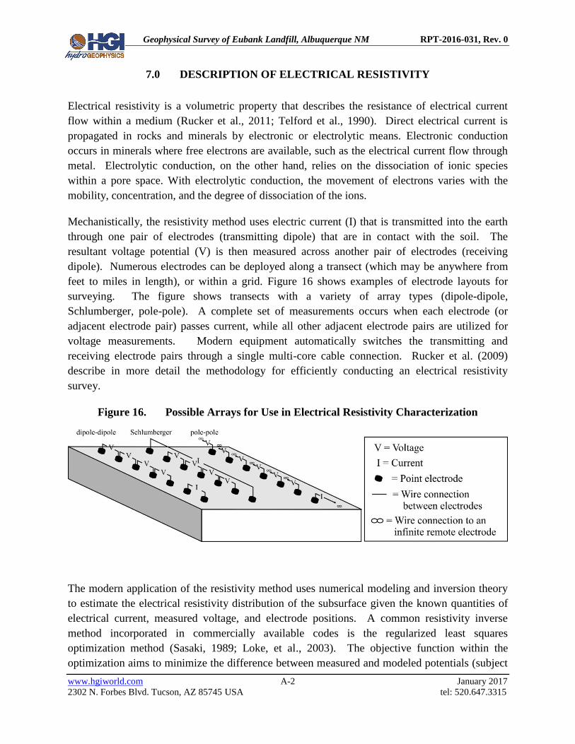
Figure 15. Line 7 Electrical Resistivity Comparison with EM & Mag Slices. ........................ 36 Figure 16. Possible Arrays for Use in Electrical Resistivity Characterization ...................... A-2

Geophysical Survey of Los Angeles Landfill, Albuquerque NM RPT-2016-031, Rev. 0
www.hgiworld.com 1 January, 2017
2302 N. Forbes Blvd. Tucson, AZ 85745 USA tel: 520.647.3315
1.0 INTRODUCTION
1.1 PROJECT DESCRIPTION
In November and December 2016, hydroGEOPHYSICS, Inc. (HGI) performed a multi-method
geophysical survey at a closed landfill in Albuquerque, New Mexico. This survey effort was
completed to determine the lateral extents and thickness of buried waste and the depth of cover
material over the waste at the location of the former Los Angeles Landfill. A combined
electromagnetic (EM) and magnetic (Mag) survey over the entire accessible landfill area, as well
as seven lines of two-dimensional (2D) Electrical Resistivity Tomography (ERT) were
completed. This report documents results from data acquired at the Los Angeles Landfill (LA
Landfill), one of four landfill sites surveyed using these combined geophysical methods.
1.2 SCOPE
The scope of this project includes using EM, Mag, and ERT to characterize the subsurface at the
survey site. The ground conductivity portion of the EM measurement provides a good indication
of the lateral limits of covered or closed landfill, presented in a georeferenced 2D plan view of
the electrical properties of the subsurface. The magnetic measurements are highly sensitive to
ferrous metals in the landfill, providing a high-resolution plan view map of the distribution of
ferrous metallic wastes within the landfills. The electrical resistivity imaging method results in
2D cross sections of the electrical properties of the subsurface materials, allowing the depth,
thickness, and lateral limits of the conductive wastes to be estimated, together with an estimate
of the thickness of the cover material.
1.3 OBJECTIVE
The objective of this multi-method geophysical survey was to non-invasively determine the
extent and thickness of buried waste and the depth of cover material over the waste by mapping
the electrical properties of the subsurface. This is based on the theory that generally, the
products of the decomposition of municipal solid waste are conductive, and as these mix with
precipitation and/or groundwater flow, the resulting bulk electrical properties of the wastes are
likely to be highly conductive compared to typical background bedrock geological materials.
The landfill is also expected to contain metallic debris which when imaged using magnetic
gradiometry should display contrast to undisturbed materials outside the landfill boundaries.

Geophysical Survey of Los Angeles Landfill, Albuquerque NM RPT-2016-031, Rev. 0
www.hgiworld.com 2 January, 2017
2302 N. Forbes Blvd. Tucson, AZ 85745 USA tel: 520.647.3315
2.0 BACKGROUND
2.1 SITE LOCATION
The Los Angeles landfill is located in the city of Albuquerque, New Mexico, USA. Figure 1
shows the general location of the geophysical survey site.
The Los Angeles Landfill is located at 4300 Alameda Blvd. NE. The landfill operated during the
years 1978-1983, with a total estimated waste tonnage of 2 million tons. The landfill has a
gravel parking lot, as well as some natural vegetation as cover. The site is known to contain
subsurface/surface utilities and some amount of infrastructure.
There are no available historical references for boundary and construction geometry for the Los
Angeles landfill and cover; however, tribal knowledge of the site estimates an average cover
thickness of 3 feet, and average waste depth of 35 feet. These values may vary across the site.
The total area covered by the Los Angeles landfill is approximately 77 acres.
Figure 1. General Survey Location
Aerial imagery © Google Earth 2016

Geophysical Survey of Los Angeles Landfill, Albuquerque NM RPT-2016-031, Rev. 0
www.hgiworld.com 3 January, 2017
2302 N. Forbes Blvd. Tucson, AZ 85745 USA tel: 520.647.3315
3.0 METHODOLOGY
3.1 SURVEY AREA AND LOGISTICS
EM & Mag data were acquired between 10/31/16 and 11/3/16 at high-resolution sampling with
rapid acquisition using the HGI Geophysical Operations (G.O.) Cart (Section 3.2.1). Data were
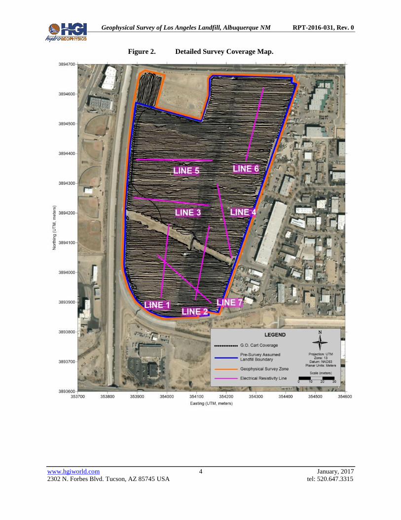
recorded continuously along survey lines to produce the coverage shown in Figure 2. The total
area covered was approximately 77 acres. The survey area had little topography and vegetation
as most of the area had been converted to a RV parking lot for the Balloon Festival. Some of the
RV parking areas contained surface and subsurface utilities and infrastructure that were likely
contributed to geophysical responses in their vicinity. The vegetation that was present on the site
was sparse could be driven over with the G.O. Cart and ATV. The only area that was unable to
be surveyed was a runoff ditch that was fenced off. The boundaries of this survey were enclosed
by a chain link fence, so we were unable to survey much beyond the landfill fenced area.
Resistivity data consisted of seven lines of data approximately 817 feet long each, totaling
approximately 5,719 feet of total line coverage. The locations of the survey lines are shown in
Figure 2 (pink lines). Table 1 lists specific parameters for the resistivity survey lines.
Prior to commencement of the geophysical survey, a general assumption existed on the location
of the boundary of the landfill. This information is posted on Figure 2 as a blue boundary line,
with extents as provided by the City of Albuquerque.
Table 1. Resistivity Line Parameters.
Line
#
Date of
Acquisition
Electrode
Spacing
(feet)
Length
(feet)
Line
Orientation
Start Position
(Easting, Northing)
UTM - meters
End Position
(Easting, Northing)
UTM - meters
1 12/5/16 10 817 S-N 353979, 3893916 354006, 3894162
2 12/7/16 10 817 S-N 354095, 3893910 354142, 3894156
3 12/6/16 10 817 W-E 353889, 3894245 354141, 3894226
4 12/7/16 10 817 S-N 354217, 3894051 354170, 3894296
5 12/6/16 10 817 W-E 353902, 3894381 354151, 3894377
6 12/8/16 10 817 S-N 354266, 3894377 354325, 3894621
7 12/8/16 10 817 NW-SE 353969, 3894058 354149, 3893898
Geophysical Survey of Los Angeles Landfill, Albuquerque NM RPT-2016-031, Rev. 0
www.hgiworld.com 4 January, 2017
2302 N. Forbes Blvd. Tucson, AZ 85745 USA tel: 520.647.3315
Figure 2. Detailed Survey Coverage Map.
Geophysical Survey of Los Angeles Landfill, Albuquerque NM RPT-2016-031, Rev. 0
www.hgiworld.com 5 January, 2017
2302 N. Forbes Blvd. Tucson, AZ 85745 USA tel: 520.647.3315
3.2 EQUIPMENT
3.2.1 G.O. Cart
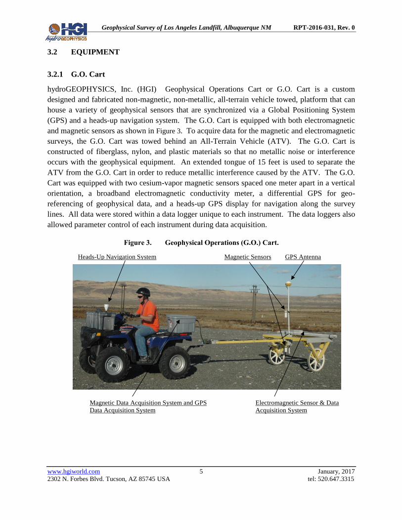
hydroGEOPHYSICS, Inc. (HGI) Geophysical Operations Cart or G.O. Cart is a custom
designed and fabricated non-magnetic, non-metallic, all-terrain vehicle towed, platform that can
house a variety of geophysical sensors that are synchronized via a Global Positioning System
(GPS) and a heads-up navigation system. The G.O. Cart is equipped with both electromagnetic
and magnetic sensors as shown in Figure 3. To acquire data for the magnetic and electromagnetic
surveys, the G.O. Cart was towed behind an All-Terrain Vehicle (ATV). The G.O. Cart is
constructed of fiberglass, nylon, and plastic materials so that no metallic noise or interference
occurs with the geophysical equipment. An extended tongue of 15 feet is used to separate the
ATV from the G.O. Cart in order to reduce metallic interference caused by the ATV. The G.O.
Cart was equipped with two cesium-vapor magnetic sensors spaced one meter apart in a vertical
orientation, a broadband electromagnetic conductivity meter, a differential GPS for geo-
referencing of geophysical data, and a heads-up GPS display for navigation along the survey
lines. All data were stored within a data logger unique to each instrument. The data loggers also
allowed parameter control of each instrument during data acquisition.
Figure 3. Geophysical Operations (G.O.) Cart.
Heads-Up Navigation System Magnetic Sensors GPS Antenna
Electromagnetic Sensor & Data
Acquisition System
Magnetic Data Acquisition System and GPS
Data Acquisition System

Geophysical Survey of Los Angeles Landfill, Albuquerque NM RPT-2016-031, Rev. 0
www.hgiworld.com 6 January, 2017
2302 N. Forbes Blvd. Tucson, AZ 85745 USA tel: 520.647.3315
3.2.1.1 Magnetic Gradiometry
A G-858G dual-sensor gradiometer (Geometrics, Inc., San Jose, CA) was used to provide
magnetic (Mag) data for the project. The instrument is commercially available and was designed
to provide detection of subsurface ferrous metals by mapping distortions to the measured
localized magnetic field. The gradiometer is easily adapted for use on the non-magnetic G.O
Cart. Dual-sensor magnetometers are called gradiometers and measure gradient of the magnetic
field; single-sensor magnetometers measure total field. The use of the two sensors on the
gradiometer allows for nulling of the earth’s magnetic field making the system highly sensitive
to subsurface ferrous metals. The gradient measurement, in this case a vertical gradient, is the
resulting difference between the top sensor and bottom sensor measurements.
The separation between the two sensors and the data acquisition and storage console is increased
using standard extension cables to cover the span between the cart and the ATV or operator. The
gradiometer console contains a serial input and necessary firmware that is used to interface with
and store GPS data. Interchangeable low voltage 12V dc gel cell batteries are used to power the
gradiometer console that is located on the ATV just behind the operator.
A daily inspection is completed by the qualified operator to ensure all components are in
satisfactory working condition. Quality assurance tests including a visual inspection, a function
test, a static response test, a vibration test, and a dynamic response test were performed daily.
3.2.1.2 Electromagnetic Induction
The GEM-2® electromagnetic instrument (Geophex Ltd, Raleigh, NC) was used to provide
electromagnetic (EM) data. The electromagnetic system is used to detect variations in
subsurface soil moisture, soil conductivity, and the presence of subsurface infrastructure
(utilities, pipes, tanks, etc.). The GEM-2 consists of a sensor housing (the “ski”), and the
electronics console. The console includes the data acquisition, rechargeable battery, and data
storage hardware. Accessories include a battery charger, carrying straps, a download cable, a
brief field guide, and manual. The console contains one DB9 serial connector for downloading
data to a PC using the manufacturer-supplied WinGEM software, and another DB9 serial
connector that accepts and records a GPS data stream. The GPS time and location are appended
to each electromagnetic data point. The instrument is commercially available and is widely used
within the geophysical arena.
The instrument was easily adapted for use on the non-magnetic G.O Cart. The instrument, which
contains a data acquisition console and an antenna ski, is lightweight and could be mounted as a
single unit on the back of the G.O. Cart. The large battery and memory capacity provided
increased field time.
® GEM-2 is a registered trademark of Geophex, Ltd.
Geophysical Survey of Los Angeles Landfill, Albuquerque NM RPT-2016-031, Rev. 0
www.hgiworld.com 7 January, 2017
2302 N. Forbes Blvd. Tucson, AZ 85745 USA tel: 520.647.3315
A daily inspection is completed by the qualified operator to ensure all components are in
satisfactory working condition. Quality assurance tests including a visual inspection, a function
test, a static response test, a vibration test, and a dynamic response test were performed daily.
3.2.1.3 G.O. Cart GPS
The Novatel Smart V1 GPS is used on the G.O. Cart for acquiring Global Positioning System
(GPS) data which are used to geo-reference (spatially locate) specific data points for the G.O.
Cart data. The exact location of the individual data points is important in order to correlate the
physical location of any interpreted anomalies that might need further investigation. The GPS
equipment used to interface with the G.O. Cart instruments provides a lateral accuracy of less
than 3.3 feet (1.0 meter) and a vertical accuracy less than approximately 6.6 feet (2.0 meters).
The geophysical instruments both require a real time GPS data stream that is stored directly
within the respective geophysical instruments. This process allows a common spatial reference
for multiple geophysical data sets. The G.O. Cart includes a GEM-2 electromagnetic instrument
and a G-858G dual-sensor gradiometer instrument. Both instruments are capable of interfacing
with a GPS instrument that provides an NMEA-compatible data stream. The G.O Cart travels at
approximately 3 to 4 miles per hour, which requires a GPS sampling and output rate of 1 Hz
(1 second). The line spacing varied between 7 and 10 feet and was influenced by site conditions
at the time of the survey such as vegetation, extreme topography or debris fields. Elevation data
are not currently used for processing electromagnetics or magnetics data; therefore, no accuracy
requirements exist. The magnetic instrument is sensitive to ferrous and/or magnetic material.
Therefore, a GPS that has the smallest magnetic footprint is advantageous as it reduces
environment noise. Geometrics, Inc., the manufacturer of the selected gradiometer, performed
rigorous testing with the Novatel Smart V1 GPS. The system provides the smallest magnetic
footprint as tested by Geometrics. The Smart V1 GPS provides the necessary accuracy without
any post processing or the need for a base-station GPS. A GPS positional check is completed at
the beginning of each day to ensure the GPS unit has no or minimal drift of data and is within 5
feet of the original calibration.
3.2.2 Resistivity
Data were collected using a Supersting™ R8 multichannel electrical resistivity system
(Advanced Geosciences, Inc. (AGI), Austin, TX) and associated cables, electrodes, and battery
power supply. The Supersting™ R8 meter is commonly used in surface geophysical projects and
has proven itself to be reliable for long-term, continuous acquisition. The stainless steel
electrodes were laid out along lines with a constant electrode spacing of approximately 10 feet (3
meters). Multi-electrode systems allow for automatic switching through preprogrammed
combinations of seven electrode measurements.
Geophysical Survey of Los Angeles Landfill, Albuquerque NM RPT-2016-031, Rev. 0
www.hgiworld.com 8 January, 2017
2302 N. Forbes Blvd. Tucson, AZ 85745 USA tel: 520.647.3315
3.2.2.1 Handheld GPS
Positional data for the resistivity lines were acquired via a handheld Garmin GPS unit.
Topographical data were incorporated into the 2D resistivity inversion modeling routines.
3.3 DATA CONTROL AND PROCESSING
3.3.1 Quality Control
All data were given a preliminary assessment for quality control (QC) in the field to assure
quality of data before progressing the survey. Following onsite QC, all data were transferred to
the HGI server for storage and detailed data processing and analysis. Each line or sequence of
acquisition was recorded with a separate file name. Data quality was inspected and data files
were saved to designated folders on the server. Raw data files were retained in an unaltered
format as data editing and processing was initiated. Daily notes on survey configuration,
location, equipment used, environmental conditions, proximal infrastructure or other obstacles,
and any other useful information were recorded during data acquisition and were saved to the
HGI Tucson server. The server was backed up nightly and backup tapes were stored at an offsite
location on a weekly and monthly basis.
3.3.2 G.O Cart Data Processing
Appropriately sized grids were established within the area of concern in accordance with maps of
the area. At the end of each day, data were downloaded and processed to a preliminary level in
order to assure data quality.
3.3.2.1 Magnetic Gradiometry
Time, date, and magnetic data were stored within a data logger and downloaded to a laptop PC
for processing. Magnetic data were processed using MAGMAPPER software. The raw data are
downloaded to a computer and then the GPS data are integrated with the magnetic data to
provide sub-meter accuracy. There are several options that are employed to remove any spikes
in the data set from anomalous data points. In addition, data are corrected for diurnal changes by
normalizing to a local base magnetometer. Data are reviewed on a daily basis with emphasis on
making sure the data quality is good. As the survey progressed, each new day was added into the
existing data base to ensure coherency among the whole dataset. There are typical offsets from
one day to the next and to ensure that the whole dataset was on the same datum we collected
calibration lines at several times during the day; in the morning, and at about every 3 hours when
there was a battery change. Each dataset collected was corrected to the first day’s calibration
line using a calculated correction factor.
Geophysical Survey of Los Angeles Landfill, Albuquerque NM RPT-2016-031, Rev. 0
www.hgiworld.com 9 January, 2017
2302 N. Forbes Blvd. Tucson, AZ 85745 USA tel: 520.647.3315
3.3.2.2 Electromagnetic Induction
Multiple frequencies were acquired for the electromagnetic data and each were processed and
analyzed. Both in-phase and quadrature data were acquired at 3 frequencies ranging from 5 kHz
to 20 kHz. These electromagnetic data were processed using the WinGEM Software as provided
by the manufacturer and an electrical conductivity value was calculated. The EM conductivity
and EM in-phase data were selected for final processing and presentation. The EM conductivity
data is more sensitive to soil conductivity (electrical properties) changes, while the EM in-phase
data is more sensitive to metal in the subsurface. For the purposes of this survey, all frequencies
were reviewed and there was virtually no difference in the interpretation of the datasets, so only
the 10 kHz data are presented. A similar process to the mag dataset is used to integrate the GPS
and correct each dataset against the calibration line.
3.3.2.3 EM & Mag Plotting
The EM and Mag data were gridded and color contoured in Surfer (Golden Software, Inc.). The
combined EM and Mag datasets, after being compensated for the calibration set, were combined
into one master file with approximately 1 million data points in each file. The Kriging gridding
algorithm was used within the Surfer software. This algorithm is good for large datasets and
honors the actual raw data very well without adding in artificial character to the datasets.
3.3.3 Resistivity Data Processing
The geophysical data for the resistivity survey, including measured voltage, current,
measurement (repeat) error, and electrode position, were recorded digitally with the AGI
SuperSting R8 resistivity meter. Quality control both in-field and in-office was performed
throughout the survey to ensure acceptable data quality. Data were assessed and data removal
was performed based on quality standards and degree of noise/other erroneous data. Edited data
were inverted and the results plotted for final presentation and analysis.
The raw data were evaluated for measurement noise. Those data that appeared to be extremely
noisy and fell outside the normal range of accepted conditions were manually removed within an
initial Excel spreadsheet analysis. Examples of conditions that would cause data to be removed
include, negative or very low voltages, high-calculated apparent resistivity, extremely low
current, and high repeat measurement error. Secondary data removal occurred for some of the
lines via the RMS error filter built in to the RES2DINVx64 software. RMS error filter runs were
performed removing no greater than 5% of the data, and were initiated to bring the final RMS
value down to 5% or below based on model convergence standards (see section 3.3.3.1 for more
details).

Geophysical Survey of Los Angeles Landfill, Albuquerque NM RPT-2016-031, Rev. 0
www.hgiworld.com 10 January, 2017
2302 N. Forbes Blvd. Tucson, AZ 85745 USA tel: 520.647.3315
3.3.3.1 2D Resistivity Inversion
RES2DINVx64 software (Geotomo, Inc.) was used for inverting individual lines in two
dimensions. RES2DINV is a commercial resistivity inversion software package available to the
public from www.geoelectrical.com. An input file was created from the initial edited resistivity
data and inversion parameters were chosen to maximize the likelihood of convergence. It is
important to note that up to this point, no resistivity data values had been manipulated or
changed, such as smoothing routines or box filters. Noisy data had only been removed from the
general population.
The inversion process followed a set of stages that utilized consistent inversion parameters to
maintain consistency between each model. Inversion parameter choices included the starting
model, the inversion routine (robust or smooth), the constraint defining the value of smoothing
and various routine halting criteria that automatically determined when an inversion was
complete. Convergence of the inversion was judged whether the model achieved an RMS of less
than 5% within three to five iterations.
Additional data editing was performed for some of the lines using the RMS error filter with
RES2DINVx64. This option provides a secondary means of removing bad data points from the
data set; the RES2D program displays the distribution of the percentage difference between the
logarithms of the observed and calculated apparent resistivity values in the form of a bar chart. It
is expected the “bad” data points will have relatively large “errors”, for example above 100
percent. Points with large errors can be removed and a new input file is created omitting these
points based on the cut-off error limit selected. The data are then re-run through the inversion
routine, and named with the naming convention (_i, _ii) to denote the filter trial number.
3.3.3.2 2D Resistivity Plotting
The inverted data were output from RES2DINV into a .XYZ data file and were gridded and
color contoured in Surfer (Golden Software, Inc.). Where relevant, intersecting features were
plotted on the resistivity section to assist in data analysis. Qualified in-house inversion experts
subjected each profile to a final review.
Geophysical Survey of Los Angeles Landfill, Albuquerque NM RPT-2016-031, Rev. 0
www.hgiworld.com 11 January, 2017
2302 N. Forbes Blvd. Tucson, AZ 85745 USA tel: 520.647.3315
4.0 RESULTS
4.1 GENERAL DISCUSSION
The analysis of the EM & Mag results is based on the anticipated contrast in electrical properties
between the conductive (low resistivity) landfill materials and the more resistive natural
background materials. Generally, the products of the decomposition of waste are conductive,
and as these mix with precipitation and/or groundwater flow, the resulting bulk electrical
properties of the wastes are likely to be highly conductive compared to typical natural
background materials. Metal waste within the landfill will also be electrically conductive. The
electromagnetic and magnetic survey methods via the G.O. Cart result in high-resolution 2D plan
view maps of the electrical properties of the subsurface materials, allowing the lateral limits of
the landfill to be estimated.
The magnetic measurements, and the EM in-phase measurements, are highly sensitive to bulk
metals in the landfill, ferrous and non-ferrous. This can provide a high-resolution map of the
distribution of metallic wastes within the landfills, for example 55-gallon steel drums that can
often contain hazardous wastes. The EM conductivity measurements would be expected to be
more susceptible to moisture content and other conductive materials (clays, leachate, etc.), with
the moisture in contact with waste materials of the landfill expected to be of increased
conductivity.
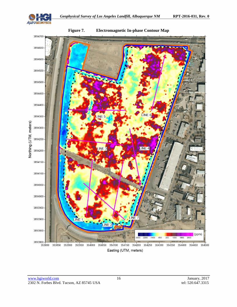
Figure 4 shows the results of the EM conductivity (sensitive to bulk conductivity changes), EM
in-phase (sensitive to bulk metal), and Mag (sensitive to ferrous metal only) survey for the whole
survey site. Magnetic data are plotted as magnetic field vertical gradient, measured in nanoteslas
per meter (nT/m). Red and purple hues indicate highest anomalous areas, while green hues are
more representative of background values. The data show heterogeneity throughout the survey
site, generally within the assumed landfill boundaries.
The results of the EM survey are plotted as 10 kHz in-phase data in parts per million (ppm) and
10 kHz conductivity data in millisiemens per meter (mS/m). In the EM conductivity results, tan
to orange hues indicate anomalous areas, green hues represent background values, and pink hues
represent lowest values that are least likely to contain high moisture. The EM in-phase results
display red to purple hues indicating anomalous areas, and blue hues representing background
values. The data show heterogeneity throughout the survey site, generally within the assumed
landfill boundaries.
Generally speaking, the magnetic response patterns are in congruence with the EM results. It is
important to note that the vertical gradient magnetic method is more sensitive to near surface
ferrous metal while the EM in-phase method is sensitive to bulk metal (ferrous and non-ferrous)
across a greater depth of investigation. As a result, EM in-phase data tend to group individual
Geophysical Survey of Los Angeles Landfill, Albuquerque NM RPT-2016-031, Rev. 0
www.hgiworld.com 12 January, 2017
2302 N. Forbes Blvd. Tucson, AZ 85745 USA tel: 520.647.3315
metal objects into larger and more diffuse bodies, whereas vertical gradient responses tend to
image smaller more individual metal objects. The two methods therefore, provide a crude means
of differentiating waste constituents. Data for the complete survey site, as well as the results of
the resistivity transects, are discussed in detail in the following sections.
The inverse model results for the electrical resistivity survey lines are presented as two-
dimensional (2D) profiles. Common color contouring scales are used for all of the lines to
provide the ability to compare anomalies from line to line. Electrically conductive (low
resistivity) subsurface regions are represented by cool hues (purple to blue) and electrically
resistive regions are represented by warm hues (orange to brown).
The objective of the survey is to geophysically characterize heterogeneities in the subsurface that
can indicate contrasts in electrical conductivity or metallic content. As such, within the
resistivity profiles, the zones of lower resistivity (higher conductivity) would be assumed to be
within the landfill, while contrasting higher resistivity would be expected to persist in the outer
undisturbed materials.
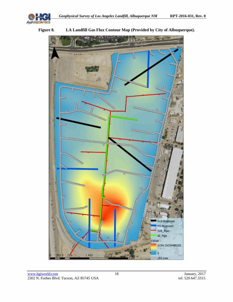
An additional objective at the LA Landfill site was to investigate any potential correlation
between the geophysical survey results and methane fluxes across the site. A number of the
electrical resistivity survey lines were located to target the area of elevated methane flux
associated with the southern portion of the landfill (Figure 8).

Geophysical Survey of Los Angeles Landfill, Albuquerque NM RPT-2016-031, Rev. 0
www.hgiworld.com 13 January, 2017
2302 N. Forbes Blvd. Tucson, AZ 85745 USA tel: 520.647.3315
Figure 4. Contoured Electromagnetics and Magnetics Map

Geophysical Survey of Los Angeles Landfill, Albuquerque NM RPT-2016-031, Rev. 0
www.hgiworld.com 14 January, 2017
2302 N. Forbes Blvd. Tucson, AZ 85745 USA tel: 520.647.3315
Figure 5. Magnetic Vertical Gradient Contour Map

Geophysical Survey of Los Angeles Landfill, Albuquerque NM RPT-2016-031, Rev. 0
www.hgiworld.com 15 January, 2017
2302 N. Forbes Blvd. Tucson, AZ 85745 USA tel: 520.647.3315
Figure 6. Electromagnetic Conductivity Contour Map
Geophysical Survey of Los Angeles Landfill, Albuquerque NM RPT-2016-031, Rev. 0
www.hgiworld.com 16 January, 2017
2302 N. Forbes Blvd. Tucson, AZ 85745 USA tel: 520.647.3315
Figure 7. Electromagnetic In-phase Contour Map
Geophysical Survey of Los Angeles Landfill, Albuquerque NM RPT-2016-031, Rev. 0
www.hgiworld.com 17 January, 2017
2302 N. Forbes Blvd. Tucson, AZ 85745 USA tel: 520.647.3315
The results of the EM and Mag surveys have been interpreted to provide a potential waste
boundary to delineate the spatial extent of the landfill, shown with a black dashed perimeter line
in Figure 4, and in greater detail in Figure 5, Figure 6, and Figure 7. This would move the
western landfill boundary to the east by approximately 82 and 131 feet (25 and 40 meters), at the
south and north ends of the landfill respectively. The southern landfill boundary would move on
average approximately 98 feet (30 meters) to the north. The eastern landfill boundary displays
an average shift of 49 feet (15 meters) to the west for the southern section of the landfill. The
northern section of the eastern landfill boundary appears to extend to pre-survey assumed landfill
boundary, which correlates to the boundary fence around the landfill property. Similarly, the top
section of the northern landfill boundary extends to the pre-survey assumed landfill boundary,
which correlates to the boundary fence around the landfill property. The section of the northern
boundary which borders the cemetery property would suggest the landfill boundary is shifted
approximately 49 feet (15 meters) to the east and south in this area.
As stated, the EM results are in general congruence with the Mag results, with high amplitude
anomalies in the EM conductivity correlating with high amplitude anomalies in the EM in-phase
results. These high amplitude anomalies tend to correlate to regions in the Mag results that
display greater heterogeneity; with a higher density of high amplitude positive and negative
anomalies. The Mag results display a number of linear high amplitude positive anomalies,
notably along the eastern edge of the landfill, trending roughly in an east-west orientation, which
are potentially a response to the landfill gas line infrastructure and RV connecting infrastructure
or utilities (Figure 5 and Figure 8).
A secondary objective of the LA Landfill geophysical mapping was related to landfill gas
production and flux across the site. There is significant infrastructure at LA Landfill related to
the capture and extraction of landfill gas and further understanding of the potential for gas
production and flux would benefit operations at the landfills. Several authors have published
research regarding a link between the electrical properties of municipal waste sites and landfill
gas concentrations and flux (Rosqvist et al, 2011; Dahlin et al, 2009). These studies tended to
indicate the landfill gas was associated with resistive regions of the surveyed areas or
correlations were observed between variations in resistivity during time-lapse monitoring and
landfill gas fluxes. It was acknowledge that there are additional factors controlling the resistivity
within the landfills and monitoring the landfills over time was likely to lead to the highest
correlations to gas flux. The EM conductivity and in-phase results do not appear to display any
correlation to the elevated landfill gas flux observed in Figure 8. This is likely based on the large
sampling volume of the EM instrument, which has the effect of averaging the electrical response
of the subsurface.
Geophysical Survey of Los Angeles Landfill, Albuquerque NM RPT-2016-031, Rev. 0
www.hgiworld.com 18 January, 2017
2302 N. Forbes Blvd. Tucson, AZ 85745 USA tel: 520.647.3315
Figure 8. LA Landfill Gas Flux Contour Map (Provided by City of Albuquerque).
Geophysical Survey of Los Angeles Landfill, Albuquerque NM RPT-2016-031, Rev. 0
www.hgiworld.com 19 January, 2017
2302 N. Forbes Blvd. Tucson, AZ 85745 USA tel: 520.647.3315
4.1.1 Line 1 Combined Method Results
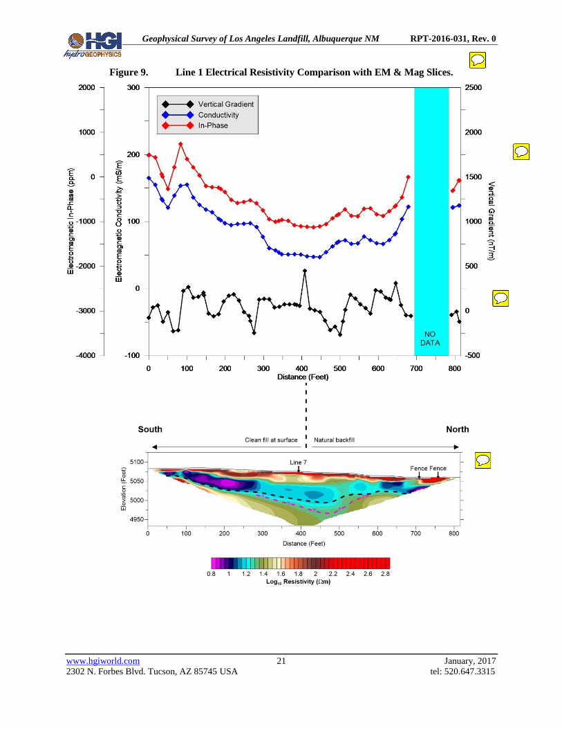
Figure 9 shows the resistivity profile for Line 1, which ran approximately south to north across
the southwest portion of the landfill, alongside Mag and EM data extracted at the location of the
resistivity line. Line 1 was collected entirely within the landfill boundary and its location was
selected by evaluating the EM and Mag results. We observe a significant level of variability in
the extracted EM and Mag readings over resistivity Line 1.
The landfill wastes typically present as a conductive target (purple and blue colors), therefore
between approximately 0 to 100 feet along the line the depth of the waste is estimated to be on
average approximately 24 feet (the base of the waste material is highlighted by the black dashed
line in Figure 9), and the thickness of the cover is around 6 to 7 feet based on the more resistive
near-surface layer (brown and red colors). Between approximately 100 to 550 feet along the line
the depth of the conductive waste feature appears to increases to approximately 88 feet, with the
cover thickness also increasing to what appears to be approximately 30 feet based on the
resistivity values. However, it is likely that a proportion of the conductive waste feature between
depths of 30 to 88 feet below ground surface (bgs) is a response to a conductive “plume” from
the waste material, which has migrated deeper within the NE survey zone (highlighted by the
magenta dashed line in Figure 9). The increase in cover material correlates well with
information communicated to HGI by the City of Albuquerque staff; which indicates that this
area has been subject to a degree of subsidence related to waste material decomposition. This
has resulted in the area being backfilled with additional cover material over the intervening
years, likely leading to the bowl shaped nature of the near-surface resistive layer. There is what
appears to be a thin more conductive layer (tan color) embedded within this increase in cover
material, between approximately 350 to 400 feet along the line and at a depth of approximately
10 feet. This may represent a perched water layer within the cover material or possibly different
fill material containing higher clay content, based on the conductive nature of the feature.
Alternatively, based on the location of this section of the survey line within the high landfill gas
flux region of the landfill, some of the apparent thickening of the cover layer is potentially a
response to the high landfill gas content of the near-surface layer. As mentioned in the previous
section a number of researchers have observed that landfill gas accumulations often appear as
resistive regions within the subsurface of solid waste sites. Therefore, a number of the more
resistive zones, located just below the near-surface highly resistive layer, along this section of the
survey line, notably 225, 270, 340, and 440 feet along the line, could be related to accumulations
or elevated flux of landfill gas. It is difficult to assign one particular interpretation to the
apparent thickening of the cover layer, either an actual thickening of the cover material based on
the subsidence and backfill or if the upper portion of the waste layer appears more resistive due
to the presence of landfill gas in this region. Indeed, this could also be a response to a
combination of the above reasons, with thicker cover layer and an elevated landfill gas
concentration and/or flux in the wastes.

Geophysical Survey of Los Angeles Landfill, Albuquerque NM RPT-2016-031, Rev. 0
www.hgiworld.com 20 January, 2017
2302 N. Forbes Blvd. Tucson, AZ 85745 USA tel: 520.647.3315
Beyond approximately 550 feet along the survey line, the depth of the conductive waste feature
decreases to approximately 40 feet, with the thickness of the cover also decreases to around 8 to
10 feet. This trend continues to the end of the coverage for this survey line, which ends just to
the north of the drainage ditch trending east-west across the landfill.
Geophysical Survey of Los Angeles Landfill, Albuquerque NM RPT-2016-031, Rev. 0
www.hgiworld.com 21 January, 2017
2302 N. Forbes Blvd. Tucson, AZ 85745 USA tel: 520.647.3315
Figure 9. Line 1 Electrical Resistivity Comparison with EM & Mag Slices.

Geophysical Survey of Los Angeles Landfill, Albuquerque NM RPT-2016-031, Rev. 0
www.hgiworld.com 22 January, 2017
2302 N. Forbes Blvd. Tucson, AZ 85745 USA tel: 520.647.3315
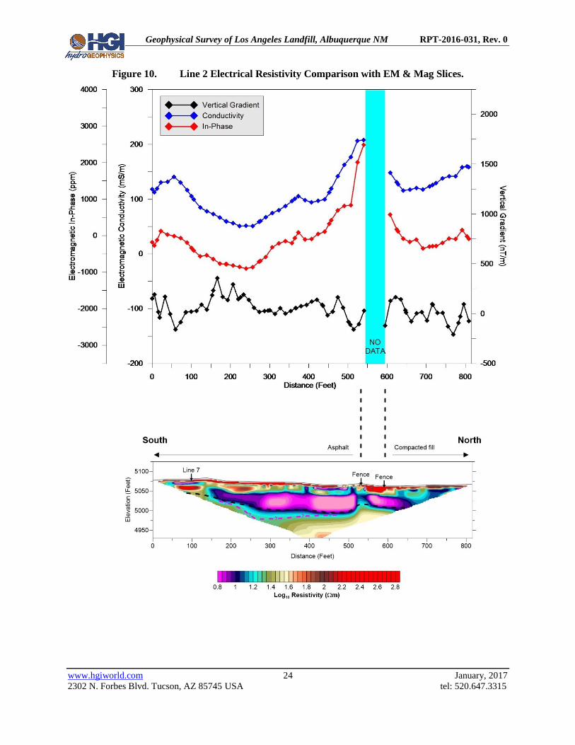
4.1.2 Line 2 Combined Method Results
Figure 10 shows the resistivity profile for Line 2, which ran approximately south to north across
the southeast portion of the landfill, alongside Mag and EM data extracted at the location of the
resistivity line. Line 2 was collected entirely within the landfill boundary, with the location
determined through evaluation of the EM and Mag results. We observe significant variability in
the extracted EM and Mag readings as expected for variable waste constituents.
Again the landfill wastes are represented by the highly conductive target along the length of the
survey line (the base of the waste material is highlighted by the black dashed line in Figure 10).
Between approximately 0 to 140 feet along the line there appears to be a thin approximately 5
feet thick cover material layer, overlying and a thin highly conductive layer approximately 5 feet
in thickness. The thin highly conductive layer may again be a response to a perched water layer
similar to that observed in Line 1. The model results then transitions to a highly resistive region
between approximately 16 to 30 feet depth (bgs). Due to the limited imaging depth and
resolution at the ends of the survey line the large contrasts of these two features may be biasing
the background resistivity of the surrounding regions. Therefore, the waste material may extend
below the resistive region but the bias from the resistive region is obscuring the return to more
conductive values. The resistive region could again be a response to elevated concentrations of
landfill gas within the wastes and cover material in the near-surface. Beyond 140 feet along the
line we observe a much better defined conductive layer, that extends to the end of the survey
line. The depth to the top of this layer remains fairly consistent, varying between 20 to 27 feet
(bgs), but the thickness of the layer increases from approximately 30 feet at 150 feet along the
line, to approximately 50 feet between 270 to 515 feet along the line. At approximately 520 feet
along the line it decreases to approximately 33 feet in thickness, and then remains fairly constant
until the end of the survey line. It is difficult to determine what portion of the response is landfill
waste and what portion is conductive leachate fluid (plume – one interpretation is highlighted by
the magenta dashed line in Figure 10).
Above the conductive layer, the upper 20 to 27 feet display a significant amount of
heterogeneity. The near-surface displays a thin resistive layer, approximately 5 feet in thickness,
which appears continuous across the length of the survey line. Between approximately 150 to
505 feet along the line we observe a similar bowl shaped, overall more resistive region to that
observe in Line 1. This could again be related to the subsidence and backfill operations within
the southern area of the landfill. Alternatively, a number of the more resistive zones, located just
below the near-surface highly resistive layer, along this section of the survey line, notably 195-
245, 295, 325, 350, 425, and 475 feet along the line, could be related to accumulations or
elevated flux of landfill gas. As mentioned in the previous section a number of researchers have
observed that landfill gas accumulations often appear as resistive regions within the subsurface
of solid waste sites. Therefore the elevated landfill gas concentrations may be increasing the
resistivity of the typically conductive wastes in these regions, explaining the heterogeneity of this
Geophysical Survey of Los Angeles Landfill, Albuquerque NM RPT-2016-031, Rev. 0
www.hgiworld.com 23 January, 2017
2302 N. Forbes Blvd. Tucson, AZ 85745 USA tel: 520.647.3315
layer. This is potentially supported by the more conductive upper layer between approximately
620 feet and the end of the survey line, where the landfill gas flux is much lower (Figure 8) and
the conductive wastes are dominating the resistivity value.
Another thin highly conductive layer, approximately 5 feet in thickness, is observed between
approximately 410 to 495 feet along the line. This layer, at a depth of approximately 10 feet
(bgs), may again be a response to a perched water layer similar to that observed at the beginning
of Line 2 and in Line 1. We also observe a highly resistive feature between approximately 545
to 595 feet along the line, extending from the ground surface to a depth of approximately 15 feet
(bgs). This corresponds to the location of the drainage ditch trending east-west across the
landfill and may be a response to the construction or materials used for this structure.
Geophysical Survey of Los Angeles Landfill, Albuquerque NM RPT-2016-031, Rev. 0
www.hgiworld.com 24 January, 2017
2302 N. Forbes Blvd. Tucson, AZ 85745 USA tel: 520.647.3315
Figure 10. Line 2 Electrical Resistivity Comparison with EM & Mag Slices.
Geophysical Survey of Los Angeles Landfill, Albuquerque NM RPT-2016-031, Rev. 0
www.hgiworld.com 25 January, 2017
2302 N. Forbes Blvd. Tucson, AZ 85745 USA tel: 520.647.3315
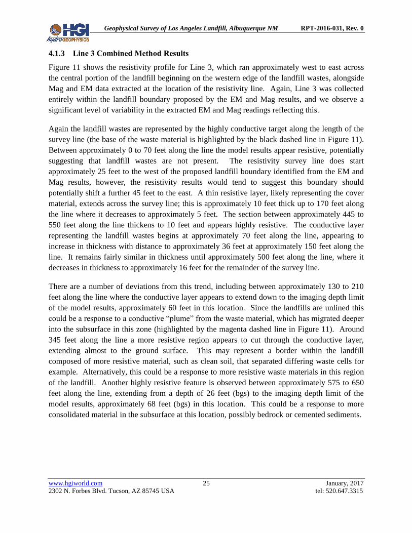
4.1.3 Line 3 Combined Method Results
Figure 11 shows the resistivity profile for Line 3, which ran approximately west to east across
the central portion of the landfill beginning on the western edge of the landfill wastes, alongside
Mag and EM data extracted at the location of the resistivity line. Again, Line 3 was collected
entirely within the landfill boundary proposed by the EM and Mag results, and we observe a
significant level of variability in the extracted EM and Mag readings reflecting this.
Again the landfill wastes are represented by the highly conductive target along the length of the
survey line (the base of the waste material is highlighted by the black dashed line in Figure 11).
Between approximately 0 to 70 feet along the line the model results appear resistive, potentially
suggesting that landfill wastes are not present. The resistivity survey line does start
approximately 25 feet to the west of the proposed landfill boundary identified from the EM and
Mag results, however, the resistivity results would tend to suggest this boundary should
potentially shift a further 45 feet to the east. A thin resistive layer, likely representing the cover
material, extends across the survey line; this is approximately 10 feet thick up to 170 feet along
the line where it decreases to approximately 5 feet. The section between approximately 445 to
550 feet along the line thickens to 10 feet and appears highly resistive. The conductive layer
representing the landfill wastes begins at approximately 70 feet along the line, appearing to
increase in thickness with distance to approximately 36 feet at approximately 150 feet along the
line. It remains fairly similar in thickness until approximately 500 feet along the line, where it
decreases in thickness to approximately 16 feet for the remainder of the survey line.
There are a number of deviations from this trend, including between approximately 130 to 210
feet along the line where the conductive layer appears to extend down to the imaging depth limit
of the model results, approximately 60 feet in this location. Since the landfills are unlined this
could be a response to a conductive “plume” from the waste material, which has migrated deeper
into the subsurface in this zone (highlighted by the magenta dashed line in Figure 11). Around
345 feet along the line a more resistive region appears to cut through the conductive layer,
extending almost to the ground surface. This may represent a border within the landfill
composed of more resistive material, such as clean soil, that separated differing waste cells for
example. Alternatively, this could be a response to more resistive waste materials in this region
of the landfill. Another highly resistive feature is observed between approximately 575 to 650
feet along the line, extending from a depth of 26 feet (bgs) to the imaging depth limit of the
model results, approximately 68 feet (bgs) in this location. This could be a response to more
consolidated material in the subsurface at this location, possibly bedrock or cemented sediments.
Geophysical Survey of Los Angeles Landfill, Albuquerque NM RPT-2016-031, Rev. 0
www.hgiworld.com 26 January, 2017
2302 N. Forbes Blvd. Tucson, AZ 85745 USA tel: 520.647.3315
Figure 11. Line 3 Electrical Resistivity Comparison with EM & Mag Slices.

Geophysical Survey of Los Angeles Landfill, Albuquerque NM RPT-2016-031, Rev. 0
www.hgiworld.com 27 January, 2017
2302 N. Forbes Blvd. Tucson, AZ 85745 USA tel: 520.647.3315
4.1.4 Line 4 Combined Method Results
Figure 12 shows the resistivity profile for Line 4, which ran approximately south to north across
the central portion of the landfill beginning on the eastern edge of the landfill wastes, alongside
Mag and EM data extracted at the location of the resistivity line. Again, Line 4 was collected
entirely within the landfill boundary proposed by the EM and Mag results, and we observe a
significant level of variability in the extracted EM and Mag readings reflecting this.
Again the landfill wastes are represented by the highly conductive target along the length of the
survey line (the base of the waste material is highlighted by the black dashed line in Figure 12).
A thin resistive layer, likely representing the cover material, extends across the survey line; this
is approximately 7 feet thick up to 165 feet along the line. Between 165 to 370 feet along the
line the cover material appears to increase to maximum of 17 feet thick, before decreasing back
to a thickness of approximately 7 feet for the remainder of the survey line. The conductive layer
representing the landfill wastes appears to increase in thickness between approximately 0 to 150
feet along the line, from approximately 10 to 22 feet thick. Between approximately 200 to 550
feet along the line the waste material thickness remains fairly similar, at approximately 30 feet.
There is a suggestion of a conductive plume from the waste material between approximately 370
to 490 feet along the line, appearing to extend down an additional 40 feet in depth (highlighted
by the magenta dashed line in Figure 12). After 550 feet along the line the thickness of the waste
material layer appears to decrease significantly, to approximately 12 feet by around 595 feet
along the line. It remains of a similar thickness until 755 feet along the line, where the
subsurface becomes more resistive potentially indicating no waste materials are present, or that
the materials change to more resistive types of waste.

Geophysical Survey of Los Angeles Landfill, Albuquerque NM RPT-2016-031, Rev. 0
www.hgiworld.com 28 January, 2017
2302 N. Forbes Blvd. Tucson, AZ 85745 USA tel: 520.647.3315
Figure 12. Line 4 Electrical Resistivity Comparison with EM & Mag Slices.

Geophysical Survey of Los Angeles Landfill, Albuquerque NM RPT-2016-031, Rev. 0
www.hgiworld.com 29 January, 2017
2302 N. Forbes Blvd. Tucson, AZ 85745 USA tel: 520.647.3315
4.1.5 Line 5 Combined Method Results
Figure 13 shows the resistivity profile for Line 5, which ran approximately west to east across
the northwest portion of the landfill, beginning on the western edge of the landfill wastes,
alongside Mag and EM data extracted at the location of the resistivity line. Again, Line 5 was
collected entirely within the landfill boundary proposed by the EM and Mag results, and we
observe a significant level of variability in the extracted EM and Mag readings reflecting this.
Again the landfill wastes are represented by the conductive target along the length of the survey
line. A thin resistive layer, likely representing the cover material, extends across the survey line;
this is approximately 8 feet thick across the length of the survey line. An obvious highly
conductive feature is observed between approximately 240 to 320 feet along the line (highlighted
by the gray cross-hatch region in Figure 13), extending from a depth of approximately 13 feet
(bgs) to the depth limit of the model (approximately 90 feet in this location). The location of this
feature also corresponds to significant responses in the EM-conductivity and EM-in-phase
profiles, both reflected as decreases in values. This is likely a response to metallic infrastructure
in the subsurface, possible a conductive pipeline or drain for example, that the resistivity survey
line crosses over. The EM-conductivity and EM-in-phase results presented in Figure 6 and
Figure 7 appear to indicate the significant decrease in values extends in a linear nature to the
north and south of the resistivity survey line, lending weight to the pipeline response. We
observe a number of highly resistive responses around this highly conductive feature in the
resistivity model results, which are likely to be artifacts of the inversion process (where the
model tries to accommodate the highly conductive response to the potential pipeline) making
interpretation problematic in this region.
The conductive layer representing the landfill wastes can be traced across the length of the
survey line (the base of the waste material is highlighted by the black dashed line in Figure 13),
though it is broken by a few smaller resistive bodies along the length. It appears to increase in
thickness between approximately 0 to 80 feet along the line, from approximately 10 to 20 feet
thick. Between approximately 80 to 615 feet along the line the waste material thickness remains
fairly similar, at approximately 25 feet. There is a suggestion of a conductive plume from the
waste material between approximately 425 to 585 feet along the line, appearing to extend down
an additional 20 feet in depth. After 615 feet along the line the thickness of the waste material
layer appears to decrease, to approximately 16 feet by around 650 feet along the line. It remains
of a similar thickness until the end of the survey line. Overall, the landfill wastes appear to be
less conductive, when compared to the previous resistivity survey lines, potentially suggesting a
difference in the wastes and/or their decomposition potential and/or decrease in overall moisture
content.
Outside of the region potentially affected by the highly conductive feature, there are a number of
resistive regions that deviate from the general conductive waste layer trend. This includes what

Geophysical Survey of Los Angeles Landfill, Albuquerque NM RPT-2016-031, Rev. 0
www.hgiworld.com 30 January, 2017
2302 N. Forbes Blvd. Tucson, AZ 85745 USA tel: 520.647.3315
appears to be a resistive break between approximately 380 to 415 feet along the line, and a
resistive region between approximately 500 to 550 feet along the line. The former may represent
a border within the landfill composed of more resistive material, such as clean soil, that
separated differing waste cells for example. Alternatively, this and the latter resistive region
could be a response to more resistive waste materials which were placed in this area of the
landfill that are more resistant to breaking down and forming conductive decomposition
products.

Geophysical Survey of Los Angeles Landfill, Albuquerque NM RPT-2016-031, Rev. 0
www.hgiworld.com 31 January, 2017
2302 N. Forbes Blvd. Tucson, AZ 85745 USA tel: 520.647.3315
Figure 13. Line 5 Electrical Resistivity Comparison with EM & Mag Slices.
Geophysical Survey of Los Angeles Landfill, Albuquerque NM RPT-2016-031, Rev. 0
www.hgiworld.com 32 January, 2017
2302 N. Forbes Blvd. Tucson, AZ 85745 USA tel: 520.647.3315
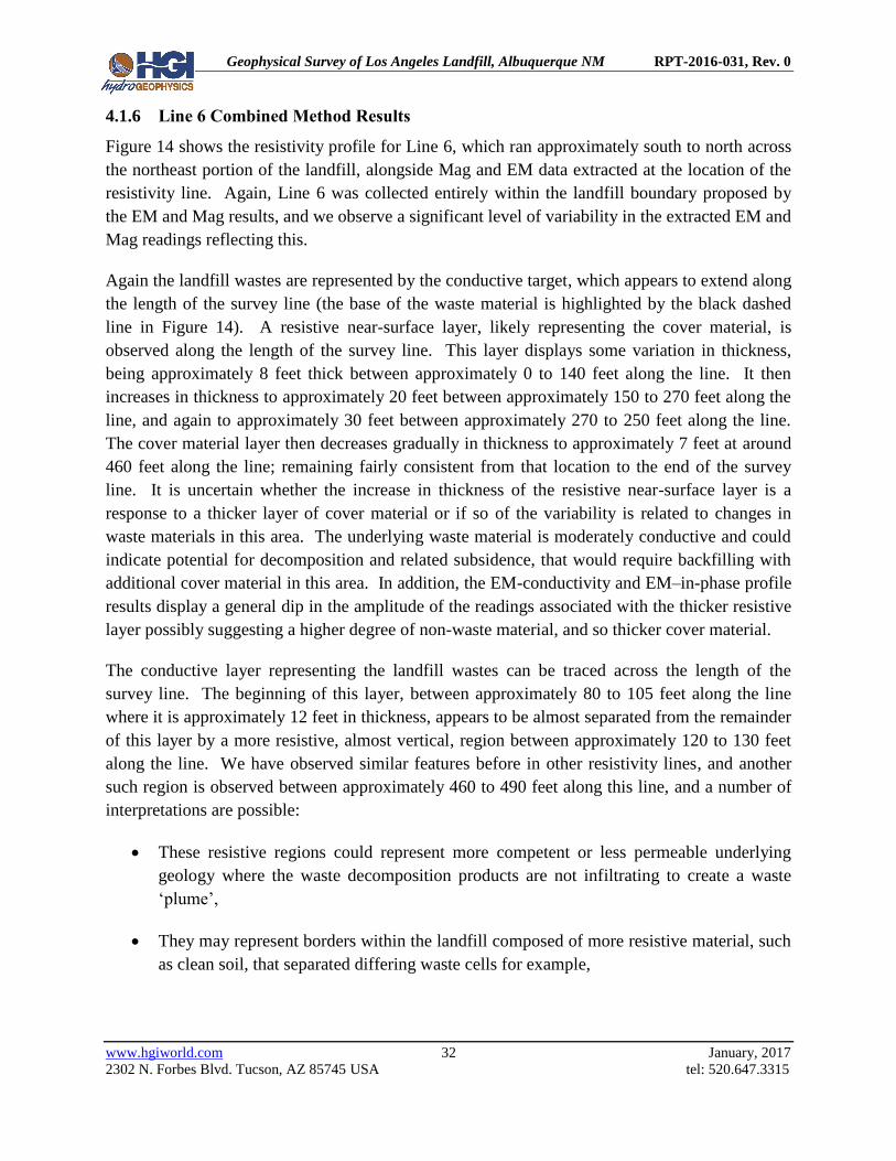
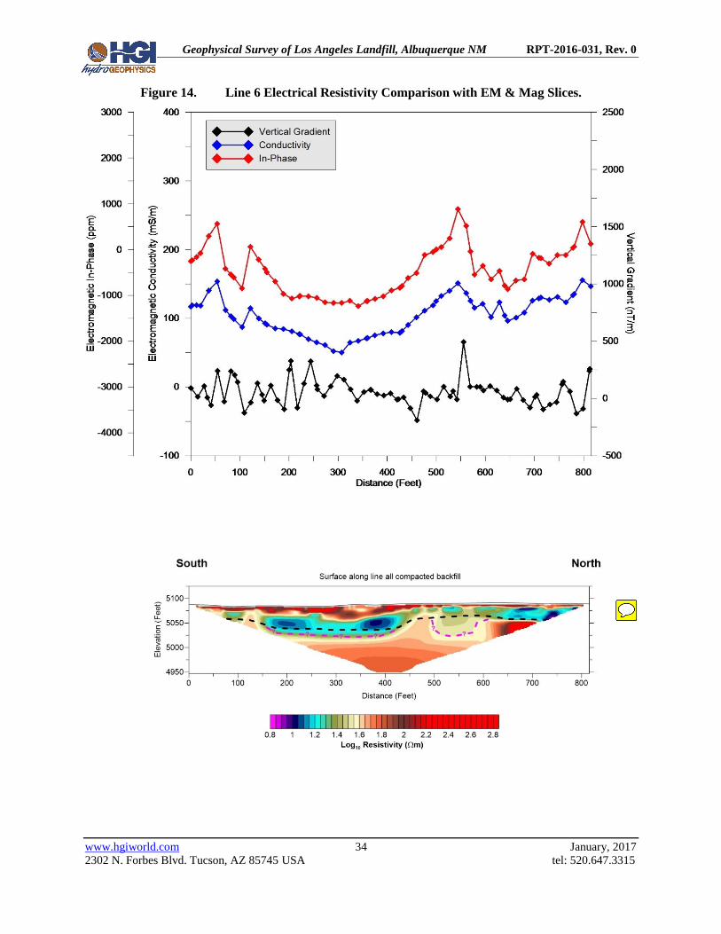
4.1.6 Line 6 Combined Method Results
Figure 14 shows the resistivity profile for Line 6, which ran approximately south to north across
the northeast portion of the landfill, alongside Mag and EM data extracted at the location of the
resistivity line. Again, Line 6 was collected entirely within the landfill boundary proposed by
the EM and Mag results, and we observe a significant level of variability in the extracted EM and
Mag readings reflecting this.
Again the landfill wastes are represented by the conductive target, which appears to extend along
the length of the survey line (the base of the waste material is highlighted by the black dashed
line in Figure 14). A resistive near-surface layer, likely representing the cover material, is
observed along the length of the survey line. This layer displays some variation in thickness,
being approximately 8 feet thick between approximately 0 to 140 feet along the line. It then
increases in thickness to approximately 20 feet between approximately 150 to 270 feet along the
line, and again to approximately 30 feet between approximately 270 to 250 feet along the line.
The cover material layer then decreases gradually in thickness to approximately 7 feet at around
460 feet along the line; remaining fairly consistent from that location to the end of the survey
line. It is uncertain whether the increase in thickness of the resistive near-surface layer is a
response to a thicker layer of cover material or if so of the variability is related to changes in
waste materials in this area. The underlying waste material is moderately conductive and could
indicate potential for decomposition and related subsidence, that would require backfilling with
additional cover material in this area. In addition, the EM-conductivity and EM–in-phase profile
results display a general dip in the amplitude of the readings associated with the thicker resistive
layer possibly suggesting a higher degree of non-waste material, and so thicker cover material.
The conductive layer representing the landfill wastes can be traced across the length of the
survey line. The beginning of this layer, between approximately 80 to 105 feet along the line
where it is approximately 12 feet in thickness, appears to be almost separated from the remainder
of this layer by a more resistive, almost vertical, region between approximately 120 to 130 feet
along the line. We have observed similar features before in other resistivity lines, and another
such region is observed between approximately 460 to 490 feet along this line, and a number of
interpretations are possible:
These resistive regions could represent more competent or less permeable underlying
geology where the waste decomposition products are not infiltrating to create a waste
‘plume’,
They may represent borders within the landfill composed of more resistive material, such
as clean soil, that separated differing waste cells for example,
Geophysical Survey of Los Angeles Landfill, Albuquerque NM RPT-2016-031, Rev. 0
www.hgiworld.com 33 January, 2017
2302 N. Forbes Blvd. Tucson, AZ 85745 USA tel: 520.647.3315
Alternatively, they could be a response to more resistive waste materials which were
placed in this area of the landfill that are more resistant to breaking down and forming
conductive decomposition products.
Without additional groundtruthing information from drilling and sampling, etc. it is difficult to
determine which interpretation is correct. For example, the conductive layer between
approximately 150 to 430 feet along the line is approximately 37 feet in thickness, but extends
almost 60 feet (bgs) due to the thick over material layer in this location. However, it may be that
the waste material is concentrated in the upper 20 feet of this layer, where we observe the highly
conductive values, with the lower remaining portion related to a conductive plume from the
decomposition products (highlighted by the magenta dashed line in Figure 14). In a similar
manner, the section of the conductive layer between approximately 450 feet along the line and
the end of the survey line is on average 20 feet in thickness, with the apparent thickening of this
layer between approximately 510 to 590 feet associated with a conductive plume.
Geophysical Survey of Los Angeles Landfill, Albuquerque NM RPT-2016-031, Rev. 0
www.hgiworld.com 34 January, 2017
2302 N. Forbes Blvd. Tucson, AZ 85745 USA tel: 520.647.3315
Figure 14. Line 6 Electrical Resistivity Comparison with EM & Mag Slices.

Geophysical Survey of Los Angeles Landfill, Albuquerque NM RPT-2016-031, Rev. 0
www.hgiworld.com 35 January, 2017
2302 N. Forbes Blvd. Tucson, AZ 85745 USA tel: 520.647.3315
4.1.7 Line 7 Combined Method Results
Figure 15 shows the resistivity profile for Line 7, which ran approximately northwest to
southeast across the southern portion of the landfill, alongside Mag and EM data extracted at the
location of the resistivity line. Again, Line 7 was collected entirely within the landfill boundary
proposed by the EM and Mag results, and we observe a significant level of variability in the
extracted EM and Mag readings reflecting this. This line was positioned to further investigate
the area of elevated landfill gas flux and the possible perched water observed in Line 2.
Line 7 crosses Line 1 around 100 feet along the line, and we observe a good agreement between
the two model results. Both display a near-surface resistive layer, approximately 30 feet in
thickness, likely representing the cover material, overlying the more conductive waste material.
We have a limited imaging depth at this location in Line 7 and so the model results only display
a small section of the conductive layer from the waste materials. However, as we progress
further along the line to the southwest, and the imaging depth increases, we observe the
conductive layer resolved much better (the base of the waste material is highlighted by the black
dashed line in Figure 15). We observe significant variation in the thickness of this layer;
approximately 46 feet thick between approximately 175 to 310 feet along the line, decreasing to
approximately 25 feet between approximately 315 to 375 feet along the line. Increasing
significantly to approximately 65 feet thick between approximately 385 to 545 feet along the
line, before decreasing to an average of 25 feet for the remainder of the line. Once again, these
significant increases are likely related to a conductive plume related to the decomposition
products extending into the underlying native strata, as is potentially reflected in the model
results of Lines 1 and 2 as well (highlighted by the magenta dashed line in Figure 15). The
southern portion of the landfill has been subjected to subsidence as the landfill wastes break
down, indicating the potential for decomposition products to be migrating in the subsurface.
Where Line 7 crosses Line 2, around 590 feet along the line, we again observe a good agreement
between the two model results. Line 7 also displays a thin highly conductive layer, just below
the resistive near-surface cover material layer, which may represent a perched water layer in this
location. A similar feature is also observed between approximately 420 to 480 feet along the
line, at the same depth, which could indicate another perched water layer. In addition, beneath
the highly conductive layer we also observed the resistive region, which again could be a
response to elevated concentrations of landfill gas within the wastes and cover material in the
near-surface. A number of additional resistive regions within the conductive layer are observed,
notably around 145 and 450 feet along the line, which possibly indicate areas where the landfill
gas is accumulating in this high flux area of the landfill.

Geophysical Survey of Los Angeles Landfill, Albuquerque NM RPT-2016-031, Rev. 0
www.hgiworld.com 36 January, 2017
2302 N. Forbes Blvd. Tucson, AZ 85745 USA tel: 520.647.3315
Figure 15. Line 7 Electrical Resistivity Comparison with EM & Mag Slices.
Geophysical Survey of Los Angeles Landfill, Albuquerque NM RPT-2016-031, Rev. 0
www.hgiworld.com 37 January, 2017
2302 N. Forbes Blvd. Tucson, AZ 85745 USA tel: 520.647.3315
5.0 CONCLUSIONS
A multi-method geophysical survey was performed at the LA Landfill in Albuquerque, New
Mexico, during November and December, 2016. The survey was performed to determine the
lateral extents and thickness of landfill waste and the thickness of the cover material. Combined
electromagnetic and magnetic surveys over the entire accessible landfill area, as well as seven
lines of 2D electrical resistivity were completed. The EM and Mag measurements provided an
indication of the lateral limits of covered landfill. The electrical resistivity imaging method
confirmed these boundary results and allowed the depth and thickness of the conductive wastes
and the thickness of the cover material to be estimated. A secondary objective at the LA Landfill
was to determine if the geophysical results displayed any correlation to landfill gas production
and flux across the site.
Based on the theory that the products of the decomposition of municipal solid waste will be
conductive compared to background geological materials, and that areas with metallic debris will
display increased magnetic gradient contrast to undisturbed materials outside the landfill
boundaries, the following observations have been made using the acquired geophysical data:
The EM and Mag data were acquired at high spatial resolution throughout the survey
site, and showed good agreement for distribution of anomalous data that would indicate
the presence of landfill waste material. The anomalous data for both methods mainly
occur within the boundary of the landfill that was assumed prior to geophysical
surveying. The data outside of this assumed boundary mostly show little anomalous
data, indicating background conditions have been mapped effectively. Combined
analysis of the EM, Mag, and Resistivity results would tend to suggest the western
assumed landfill boundary would recede by approximately 82 and 131 feet (25-40
meters), with the southern assumed landfill boundary receding by approximately 98 feet
(30 meters). The EM, Mag, and Resistivity results agreed with the majority of the
eastern and northern assumed boundaries, although these were bounded by the property
fence line in most cases. It did indicate that the southern half of the eastern assumed
boundary would recede by approximately 49 feet (15 meters).
The resistivity data provided additional imaging to support the lateral extents determined
using the EM and Mag data; with the resistivity results displaying a good alignment
where they crossed or approached the proposed landfill boundaries. The resistivity
profile results estimated the thickness of the waste to be approximately 20-25 feet (6-8
meters) at the locations of the resistivity survey lines, with cover thickness estimated on
average to be 8-10 feet (2.5-3 meters). This differs somewhat from the pre-survey
assumed values averaging 25 feet (8 meters) for waste thickness and 3 feet (1 meter) for
cover thickness. We observe some significant deviations from these averages, for
example portions of the southern area of the landfill indicated an increase in the cover
Geophysical Survey of Los Angeles Landfill, Albuquerque NM RPT-2016-031, Rev. 0
www.hgiworld.com 38 January, 2017
2302 N. Forbes Blvd. Tucson, AZ 85745 USA tel: 520.647.3315
thickness to 30 feet (9 meters) in places. This area has been subject to subsidence and
associated backfilling with additional cover material, which may explain this increase in
thickness. In addition, the conductive layer, which has been interpreted as representing
the waste materials, displays a number of increases in thickness above this average
across the majority of the survey lines. Since these landfills are not lined this could
indicate a “plume” of decomposition products that has migrated into the underlying
strata as the waste breaks down and interacts with moisture, etc.
We have identified a number of resistive regions that are generally located just below the
cover material layer within the conductive waste material. These could be related to
elevated landfill gas accumulations or flux within the waste materials, based on
relationships observed between electrical properties of these sites and landfill gas in the
literature. As the landfill gas is produce and migrates up through the waste materials, it
is assumed that it would accumulate in more porous parts of the waste or displace fluid
in the pore space, producing these more resistive regions. It is difficult to be certain
without more detailed information on these fluxes or concentrations of landfill gas in the
subsurface. One recommendation would be to repeat the resistivity measurements over
time in the areas of identified elevated landfill gas flux (like those observed in the
location of Lines 1 and 2). In this way the changes in landfill gas flux could be
correlated to changes seen in resistivity, since it is assumed other conditions controlling
the resistivity value would remain constant over time.

Geophysical Survey of Los Angeles Landfill, Albuquerque NM RPT-2016-031, Rev. 0
www.hgiworld.com 39 January, 2017
2302 N. Forbes Blvd. Tucson, AZ 85745 USA tel: 520.647.3315
6.0 REFERENCES
Constable, S. C., Parker, R. L., and Constable, C. G., 1987, Occam’s inversion: A practical
algorithm for generating smooth models from electromagnetic sounding data:
Geophysics,52, No. 3, 289-300.
Dahlin, T., Leroux, V., Rosqvist, H., Svensson, M., Lindsjo, M., Mansson, C.H., and Johansson,
S., 2009, Geoelectrical resistivity monitoring for localizing gas at landfills. Procs. Near
Surface 2009 15th
European Meeting of Environmental and Engineering Geophysics
Society, Dublin Ireland, 7-9 September.
Dey, A., and H.F. Morrison, 1979, Resistivity modeling for arbitrarily shaped three-dimensional
structures: Geophysics, 44, 753-780.
Ellis, R.G., and D.W. Oldenburg, 1994, Applied geophysical inversion: Geophysical Journal
International, 116, 5-11.
Loke, M.H., I. Acworth, and T. Dahlin, 2003, A comparison of smooth and blocky inversion
methods in 2D electrical imaging surveys: Exploration Geophysics, 34, 182-187.
Rosqvist, H., Leroux, V., Dahlin, T., Lindsjo, M., Mansson, C., and Johansson, S., 2011,
Mapping landfill gas migration using resistivity monitoring. Waste and Resource
Management, 164(1), 3-15.
Rucker, D.F., Levitt, M.T., Greenwood, W.J., 2009. Three-dimensional electrical resistivity
model of a nuclear waste disposal site. Journal of Applied Geophysics 69, 150-164.
Rucker, D.F., G.E. Noonan, and W.J. Greenwood, 2011. Electrical resistivity in support of
geologic mapping along the Panama Canal. Engineering Geology 117(1-2):121-133.
Sasaki, Y., 1989, Two-dimensional joint inversion of magnetotelluric and dipole-dipole
resistivity data: Geophysics, 54, 254-262.
Telford, W. M., Geldart, L. P., and Sherriff, R. E., 1990, Applied Geophysics (2nd
Edition),
Cambridge University Press.

Geophysical Survey of Eubank Landfill, Albuquerque NM RPT-2016-031, Rev. 0
www.hgiworld.com A-1 January 2017
2302 N. Forbes Blvd. Tucson, AZ 85745 USA tel: 520.647.3315
APPENDIX A
Description of Electrical Resistivity
Geophysical Survey of Eubank Landfill, Albuquerque NM RPT-2016-031, Rev. 0
www.hgiworld.com A-2 January 2017
2302 N. Forbes Blvd. Tucson, AZ 85745 USA tel: 520.647.3315
7.0 DESCRIPTION OF ELECTRICAL RESISTIVITY
Electrical resistivity is a volumetric property that describes the resistance of electrical current
flow within a medium (Rucker et al., 2011; Telford et al., 1990). Direct electrical current is
propagated in rocks and minerals by electronic or electrolytic means. Electronic conduction
occurs in minerals where free electrons are available, such as the electrical current flow through
metal. Electrolytic conduction, on the other hand, relies on the dissociation of ionic species
within a pore space. With electrolytic conduction, the movement of electrons varies with the
mobility, concentration, and the degree of dissociation of the ions.
Mechanistically, the resistivity method uses electric current (I) that is transmitted into the earth
through one pair of electrodes (transmitting dipole) that are in contact with the soil. The
resultant voltage potential (V) is then measured across another pair of electrodes (receiving
dipole). Numerous electrodes can be deployed along a transect (which may be anywhere from
feet to miles in length), or within a grid. Figure 16 shows examples of electrode layouts for
surveying. The figure shows transects with a variety of array types (dipole-dipole,
Schlumberger, pole-pole). A complete set of measurements occurs when each electrode (or
adjacent electrode pair) passes current, while all other adjacent electrode pairs are utilized for
voltage measurements. Modern equipment automatically switches the transmitting and
receiving electrode pairs through a single multi-core cable connection. Rucker et al. (2009)
describe in more detail the methodology for efficiently conducting an electrical resistivity
survey.
Figure 16. Possible Arrays for Use in Electrical Resistivity Characterization
The modern application of the resistivity method uses numerical modeling and inversion theory
to estimate the electrical resistivity distribution of the subsurface given the known quantities of
electrical current, measured voltage, and electrode positions. A common resistivity inverse
method incorporated in commercially available codes is the regularized least squares
optimization method (Sasaki, 1989; Loke, et al., 2003). The objective function within the
optimization aims to minimize the difference between measured and modeled potentials (subject
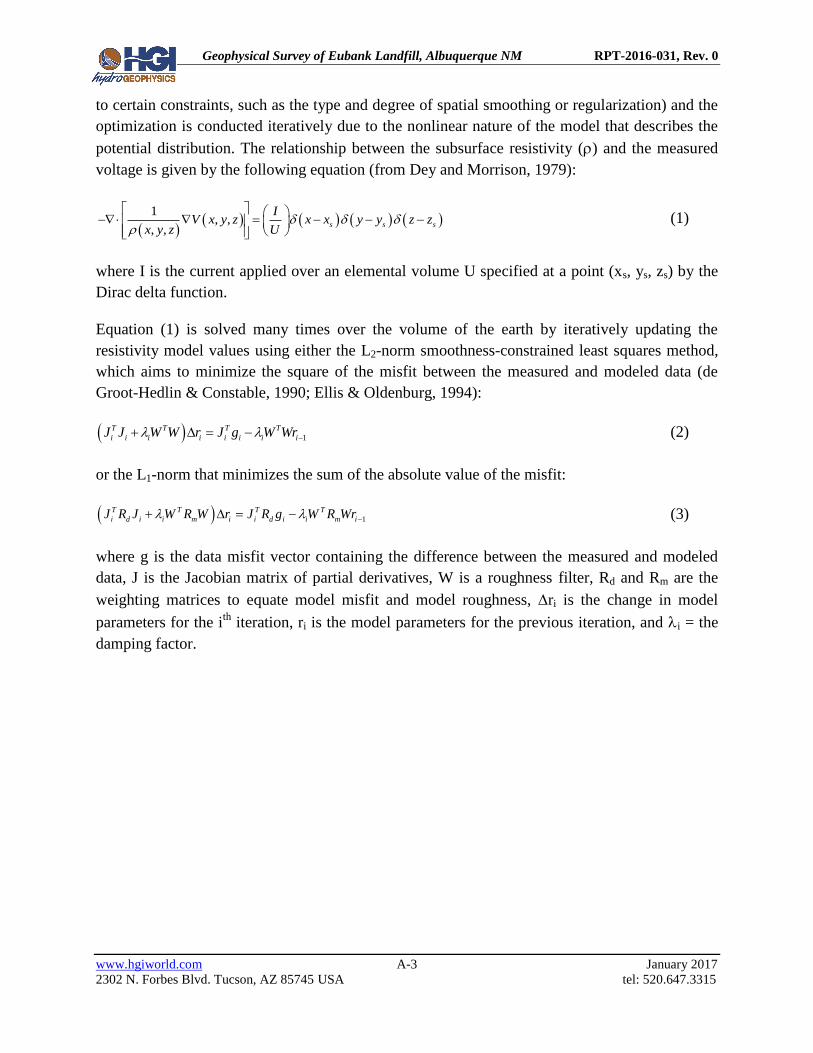
Geophysical Survey of Eubank Landfill, Albuquerque NM RPT-2016-031, Rev. 0
www.hgiworld.com A-3 January 2017
2302 N. Forbes Blvd. Tucson, AZ 85745 USA tel: 520.647.3315
to certain constraints, such as the type and degree of spatial smoothing or regularization) and the
optimization is conducted iteratively due to the nonlinear nature of the model that describes the
potential distribution. The relationship between the subsurface resistivity () and the measured
voltage is given by the following equation (from Dey and Morrison, 1979):
1, ,
, ,
s s s
IV x y z x x y y z z
x y z U (1)
where I is the current applied over an elemental volume U specified at a point (xs, ys, zs) by the
Dirac delta function.
Equation (1) is solved many times over the volume of the earth by iteratively updating the
resistivity model values using either the L2-norm smoothness-constrained least squares method,
which aims to minimize the square of the misfit between the measured and modeled data (de
Groot-Hedlin & Constable, 1990; Ellis & Oldenburg, 1994):
1
T T T T
i i i i i i i iJ J W W r J g W Wr (2)
or the L1-norm that minimizes the sum of the absolute value of the misfit:
1
T T T T
i d i i m i i d i i m iJ R J W R W r J R g W R Wr (3)
where g is the data misfit vector containing the difference between the measured and modeled
data, J is the Jacobian matrix of partial derivatives, W is a roughness filter, Rd and Rm are the
weighting matrices to equate model misfit and model roughness, ri is the change in model
parameters for the ith
iteration, ri is the model parameters for the previous iteration, and i = the
damping factor.
Geophysical Survey of Eubank Landfill, Albuquerque NM RPT-2016-031, Rev. 0
www.hgiworld.com B-1 January 2017
2302 N. Forbes Blvd. Tucson, AZ 85745 USA tel: 520.647.3315
APPENDIX B
Description of Electromagnetic Induction and Magnetic Gradiometry
Geophysical Survey of Eubank Landfill, Albuquerque NM RPT-2016-031, Rev. 0
www.hgiworld.com B-2 January 2017
2302 N. Forbes Blvd. Tucson, AZ 85745 USA tel: 520.647.3315
8.0 DESCRIPTION OF EM & MAG
8.1 MAGNETOMETRY
Magnetometry is the study of the Earth’s magnetic field and is the oldest branch of geophysics.
The Earth’s field is composed of three main parts:
1. Main field is internal (i.e., from a source within the Earth that varies slowly in time and
space)
2. Secondary field is external to the Earth and varies rapidly in time
3. Small internal fields constant in time and space are caused by local magnetic anomalies
in the near-surface crust.
Of interest to the geophysicist are the localized anomalies. These anomalies are either caused by
magnetic minerals, mainly magnetite or pyrrhotite, or buried steel and are the result of contrasts
in the magnetic susceptibility (k) with respect to the background sediments. The average values
for k are typically less than 1 for sedimentary formations and upwards to 20,000 for magnetite
minerals.
The magnetic field is measured with a magnetometer. Magnetometers permit rapid, non-contact
surveys to locate buried metallic objects and features. A one person portable field unit can be
used virtually anywhere a person can walk; although, they may be sensitive to local
interferences, such as fences and overhead wires. Airborne magnetometers are towed by aircraft
and are used to measure regional anomalies. Field-portable magnetometers maybe single- or
dual-sensor. Single-sensor magnetometers measure total field. Dual-sensor magnetometers are
called gradiometers and measure gradient of the magnetic field.
Magnetic surveys are typically conducted with two separate magnetometers. The first
magnetometer is used as a base station to record the Earth’s primary field and the diurnally
changing secondary field. The second magnetometer is used as a rover to measure the spatial
variation of the Earth’s field and may include various components (e.g., inclination, declination,
and total intensity). By removing the temporal variation and perhaps the static value of the base
station from that of the rover, one is left with a residual magnetic field that is the result of local
spatial variations only. The rover magnetometer is moved along a predetermined linear grid laid
out at the site. Readings are virtually continuous and results can be monitored in the field as the
survey proceeds.
The shortcoming with most magnetometers is that they only record the total magnetic field (F)
and not the separate components of the vector field. This shortcoming can make the
interpretation of magnetic anomalies difficult, especially since the strength of the field between
the magnetometer and target is reduced as a function of the inverse of distance between the
Geophysical Survey of Eubank Landfill, Albuquerque NM RPT-2016-031, Rev. 0
www.hgiworld.com B-3 January 2017
2302 N. Forbes Blvd. Tucson, AZ 85745 USA tel: 520.647.3315
magnetometer and target, cubed. Additional complications can include the inclination and
declination of the Earth’s field, the presence of any remnant magnetization associated with the
target, and the shape of the target.
8.2 ELECTROMAGNETIC INDUCTION
EM data is typically collected using portable ground conductivity instrumentation. Basically, a
transmitting coil induces an electromagnetic field and a receiving coil at a fixed separation
usually measures the amplitudes of the in-phase and quadrature components of the magnetic
field. Various instruments have different coil spacings and operating frequencies. Spacing and
frequency effect depth of signal penetration. Both single frequency and multi-frequency
instruments have been developed for commercial use.
Earth materials have the capacity to transmit electrical currents over a wide range. Earth
conductivity is a function of soil type, porosity, permeability, and dissolved salts. Terrain
conductivity methods seek to identify various Earth materials by measuring their electrical
characteristics and interpreting results in terms of those characteristics. EM techniques are used
to measure Earth conductivities of various soil, rock, and water components at individual survey
areas employing portable, rapid, non-invasive equipment operating at various frequencies
depending on range and depth desired.
The recorded electromagnetic field is separated into two sub-components: in-phase and
conductivity (also referred to as quadrature). The in-phase component is the most sensitive to
metallic objects and is measured in parts per million (ppm). The conductivity component is
sensitive to soil condition variations and is measured in log Siemens per meter (log S/m) using
the GEM-2 instrument.
The EM method was chosen due to the capability of mapping changes in soil conductivity that
are caused by changes in soil moisture, disruption, other conductivity changes caused by
physical property contrasts, the ability to detect metallic objects (i.e., ferrous and non-ferrous),
and the relatively rapid rate of data acquisition.
Top Related