


Languages
Pages
Legal

Generating Raster DEMfrom Mass Pointsvia TIN Streaming
Jack SnoeyinkUNC Chapel Hill
Jonathan ShewchukUC Berkeley
Tim ThirionUNC Chapel Hill
Martin IsenburgUC Berkeley
Yuanxin LiuUNC Chapel Hill
raster DEM LIDAR points
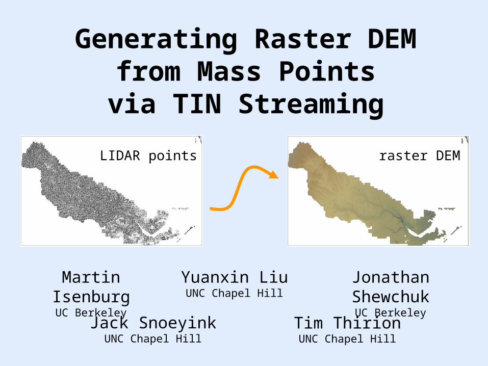
Generating DEMs from LIDAR
LIDAR points raster DEM
resampling
interpolatingtriangulating
temporary TIN
i
j
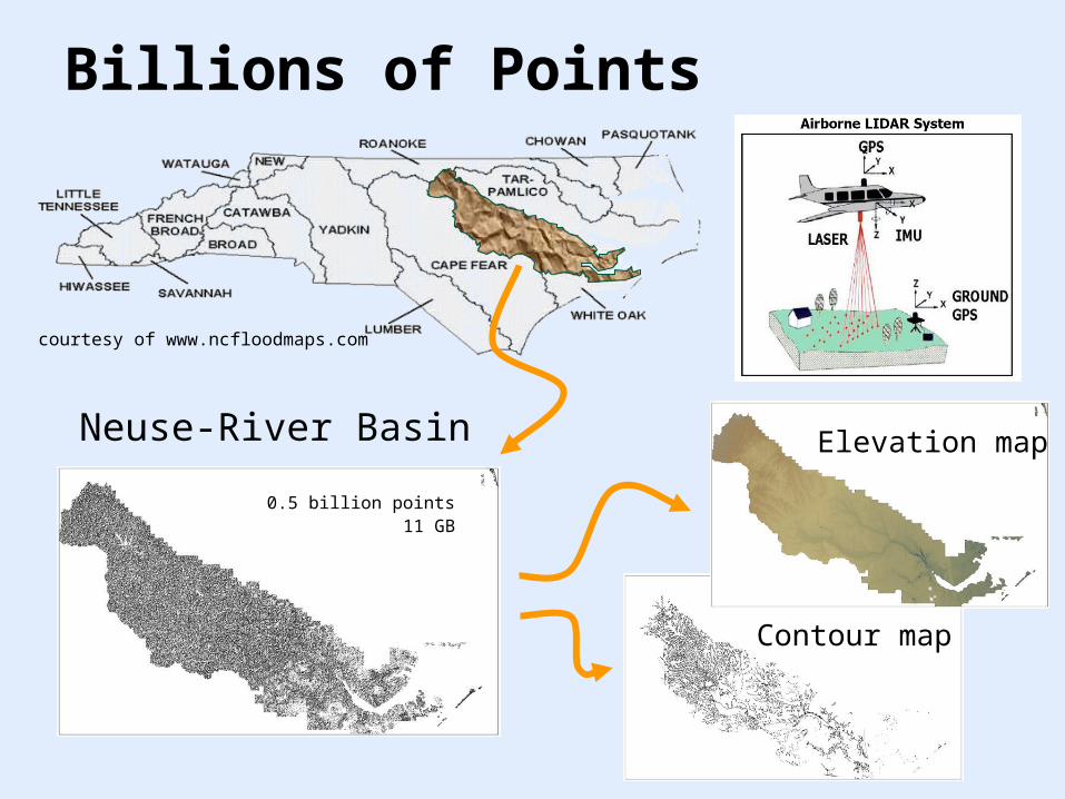
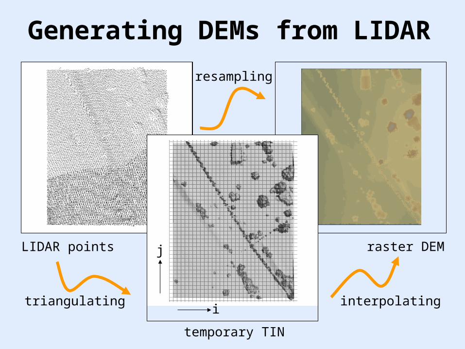
Billions of Points
courtesy of www.ncfloodmaps.com
0.5 billion points11 GB
Neuse-River Basin Elevation map
Contour map

StreamingTIN
output
output final DEMto disk
DEM Generation via TIN Streaming
small bufferin main memory
StreamingComputationof DelaunayTriangulation
read pointsfrom disk Immediate
Rasterizationof Streaming
TIN
store elevation rastersto temporary files(grouped by rows)
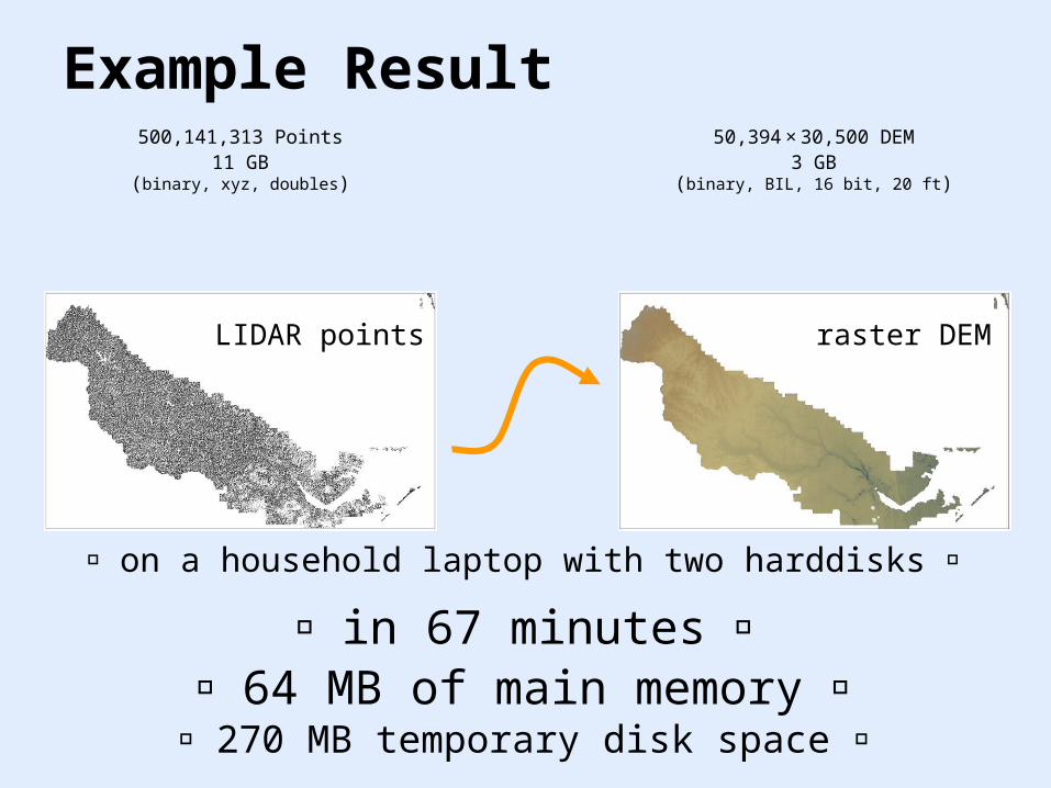
Example Result500,141,313 Points
11 GB(binary, xyz, doubles)
on a household laptop with two harddisks
50,394 × 30,500 DEM3 GB
(binary, BIL, 16 bit, 20 ft)
raster DEM LIDAR points
in 67 minutes 64 MB of main memory 270 MB temporary disk space

Related Work

• break data into (overlapping) tiles
• popular GIS packages – ArcGIS 9.1 (limit: ~ 25 million points, 1 GB)– QTModeller 4 (limit: ~ 50 million points, 1 GB)
– GRASS (limit: ~ 25 million points, 1 GB)
Rasterizing Billions of Points [Agarwal et al. ‘06]
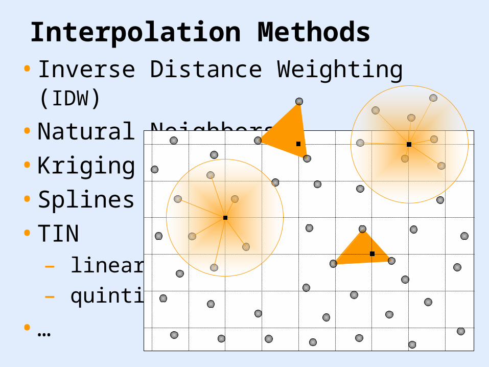
• Inverse Distance Weighting (IDW)
• Natural Neighbors
• Kriging
• Splines
• TIN– linear
– quintic
• …
Interpolation Methods

External Memory Quadtree
• rearrange points on disk into quadtree
From Point Cloud to Grid DEM: A Scalable Approach [Agarwal et al. ‘06]
• process cell– find its neighbors
– interpolate all (i,j)
– write rasters to temporary file
• sort temporary file on (i,j) & write DEM
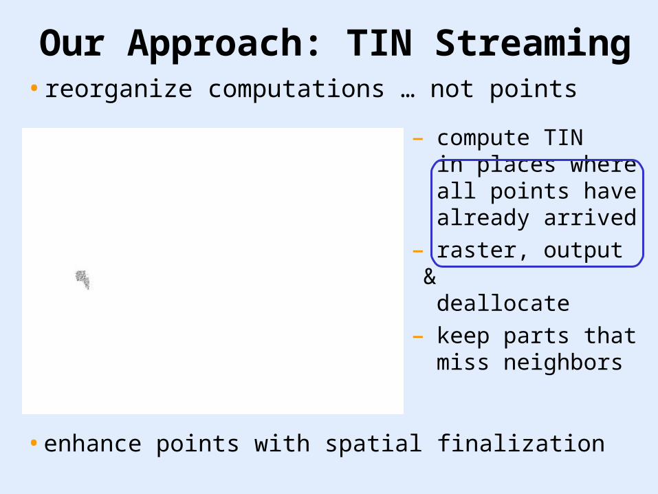
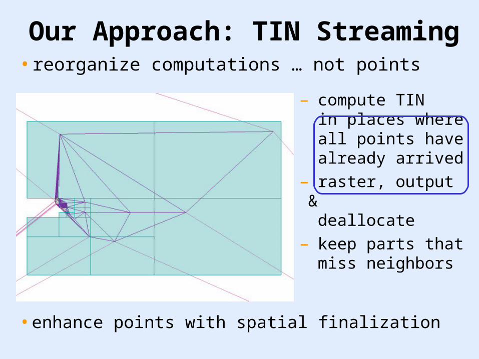
• reorganize computations … not points
Our Approach: TIN Streaming
– compute TIN in places where all points have already arrived
– raster, output & deallocate
– keep parts that miss neighbors
• enhance points with spatial finalization
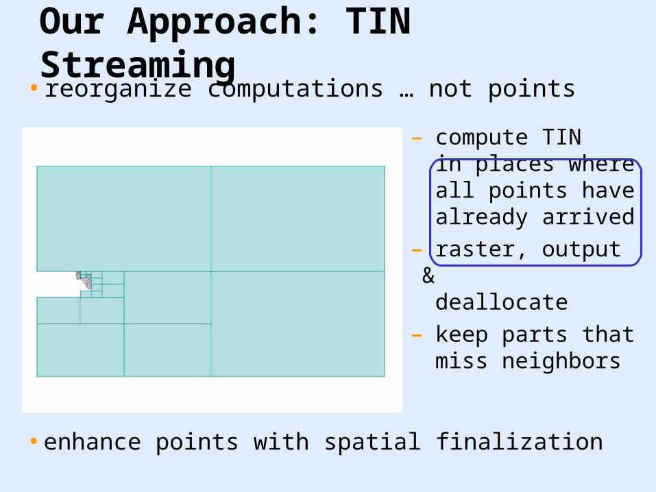
• reorganize computations … not points
Our Approach: TIN Streaming
• enhance points with spatial finalization
– compute TIN in places where all points have already arrived
– raster, output & deallocate
– keep parts that miss neighbors
• reorganize computations … not points
Our Approach: TIN Streaming
– compute TIN in places where all points have already arrived
– raster, output & deallocate
– keep parts that miss neighbors
• enhance points with spatial finalization
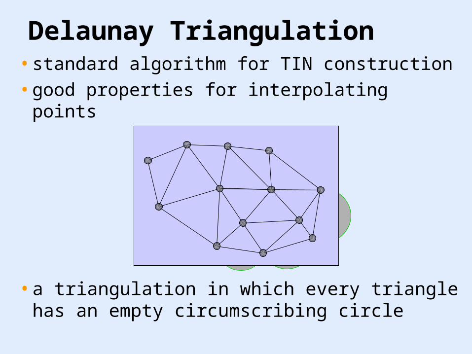
Delaunay Triangulation
• a triangulation in which every triangle has an empty circumscribing circle
• standard algorithm for TIN construction
• good properties for interpolating points
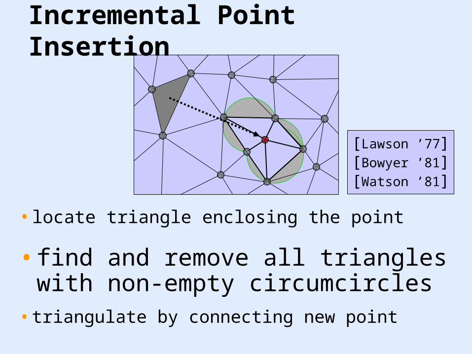
• locate triangle enclosing the point
Incremental Point Insertion
• find and remove all triangles with non-empty circumcircles
• triangulate by connecting new point
[Lawson ’77][Bowyer ’81][Watson ’81]
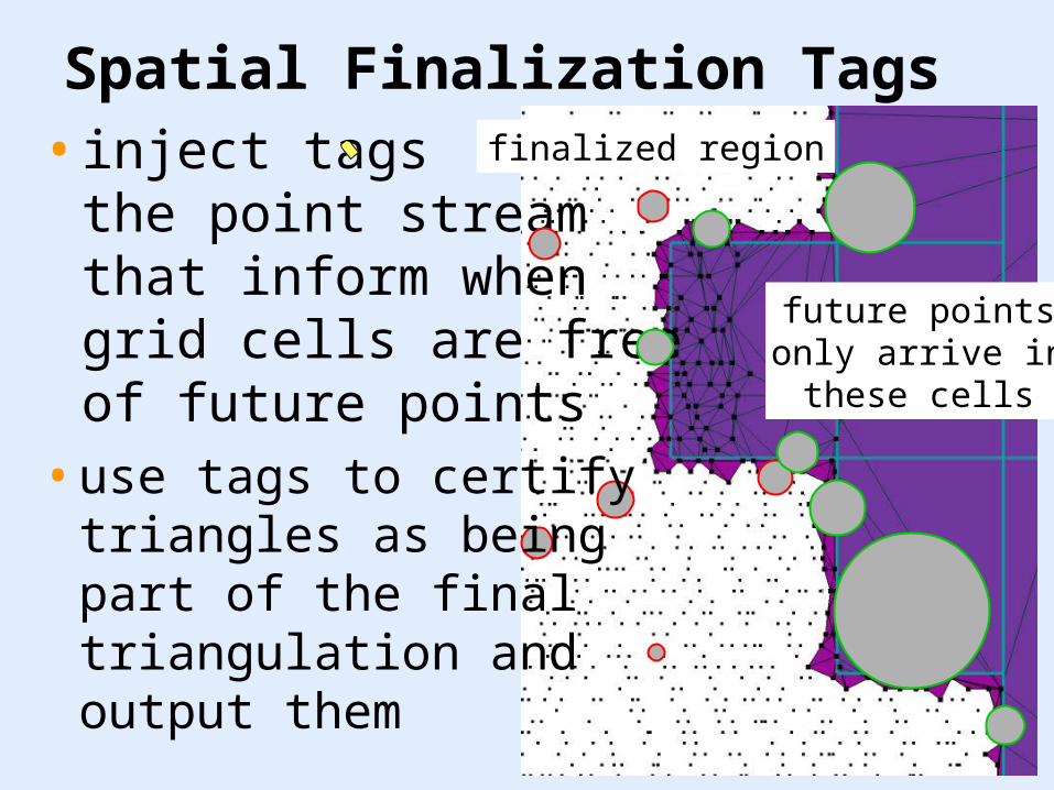
Spatial Finalization Tags• inject tags into
the point streamthat inform whengrid cells are freeof future points
finalized region
future pointsonly arrive in
these cells
• use tags to certify triangles as beingpart of the finaltriangulation andoutput them
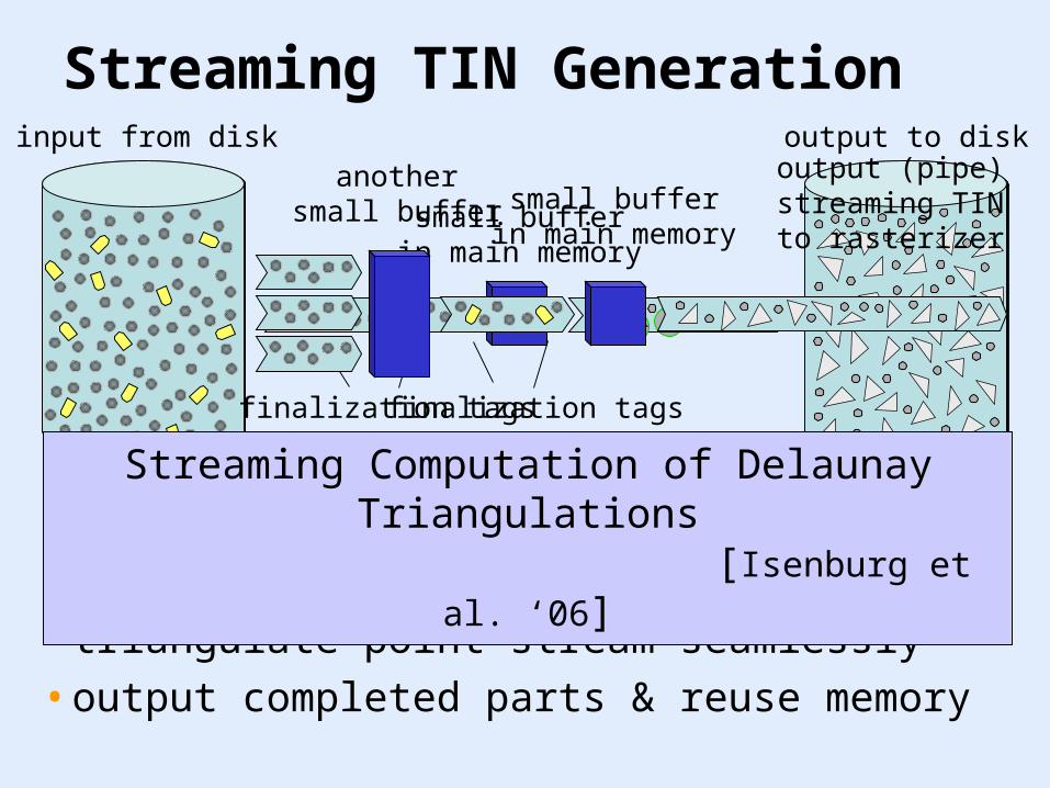
Streaming TIN Generationoutput to diskinput from disk
small bufferin main memory
• triangulate point stream seamlessly
• output completed parts & reuse memory
finalization tags
small bufferin main memory
anothersmall buffer
finalization tags
Streaming Computation of Delaunay Triangulations [Isenburg et al. ‘06]
output (pipe)streaming TINto rasterizer
input (pipe)streaming TIN
from triangulator
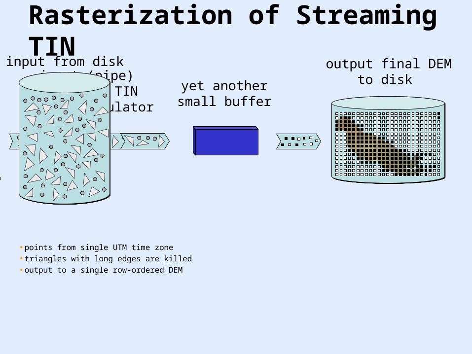
Rasterization of Streaming TINinput from disk
yet anothersmall buffer
output final DEMto disk
• points from single UTM time zone
• triangles with long edges are killed
• output to a single row-ordered DEM
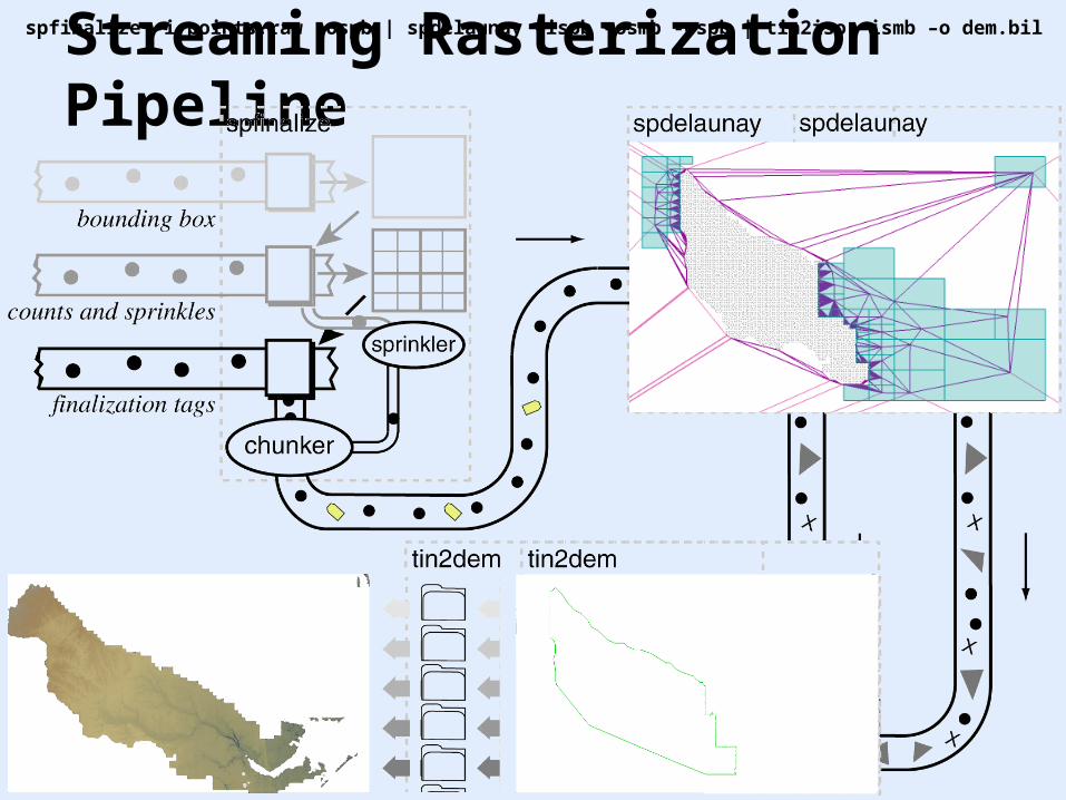
Streaming Rasterization Pipeline spfinalize -i points.raw -ospb | spdelaunay –ispb –osmb -ospb | tin2iso –ismb –o dem.bil

The Finalizer
(spfinalize)

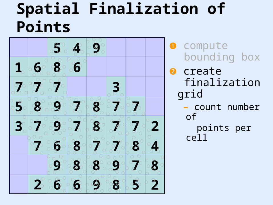
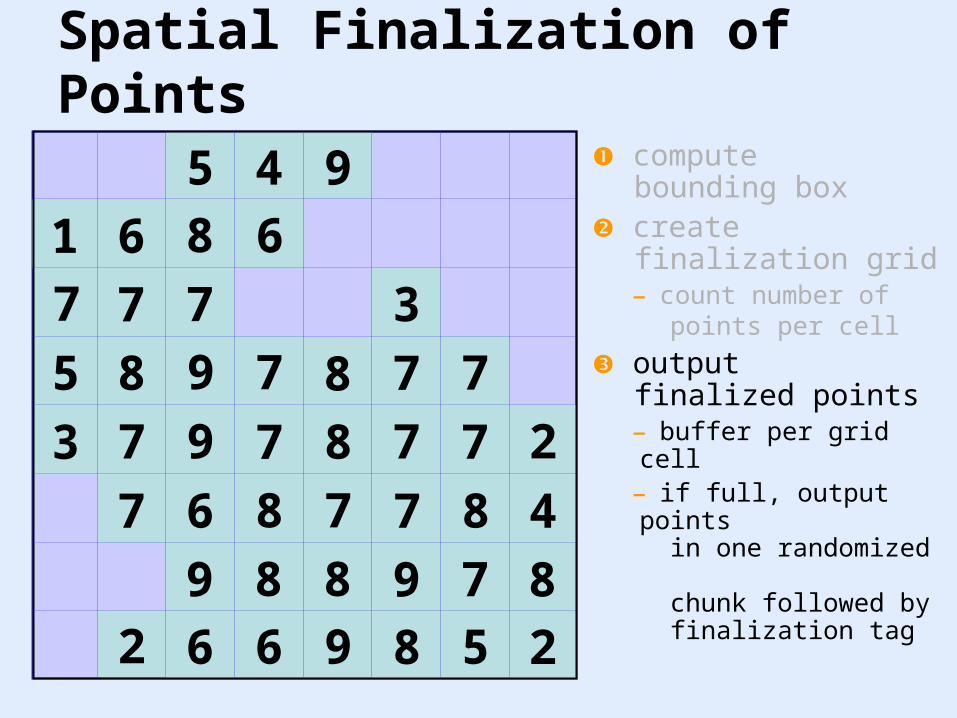
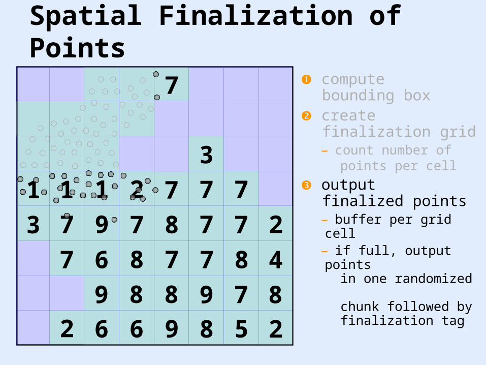
Spatial Finalization of Points
compute bounding box
2
1 13
4
5
5
1 2
6
1
8
4
7
5
5
7
1
74
1
9
7
6
4
Spatial Finalization of Points
8
9 7
9 8 5
4
8
2
7
78
86 77
73 97
889
662
7 2
7
3
75 8798
7
6
compute bounding box
create finalization grid– count number of points per cell
5
8
4
7
9
7
6
4
8
9 7
9 8 5
4
8
2
7
78
86 77
73 97
889
662
7 2
7
3
75 8798
7
61
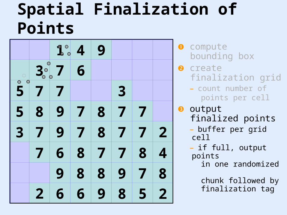
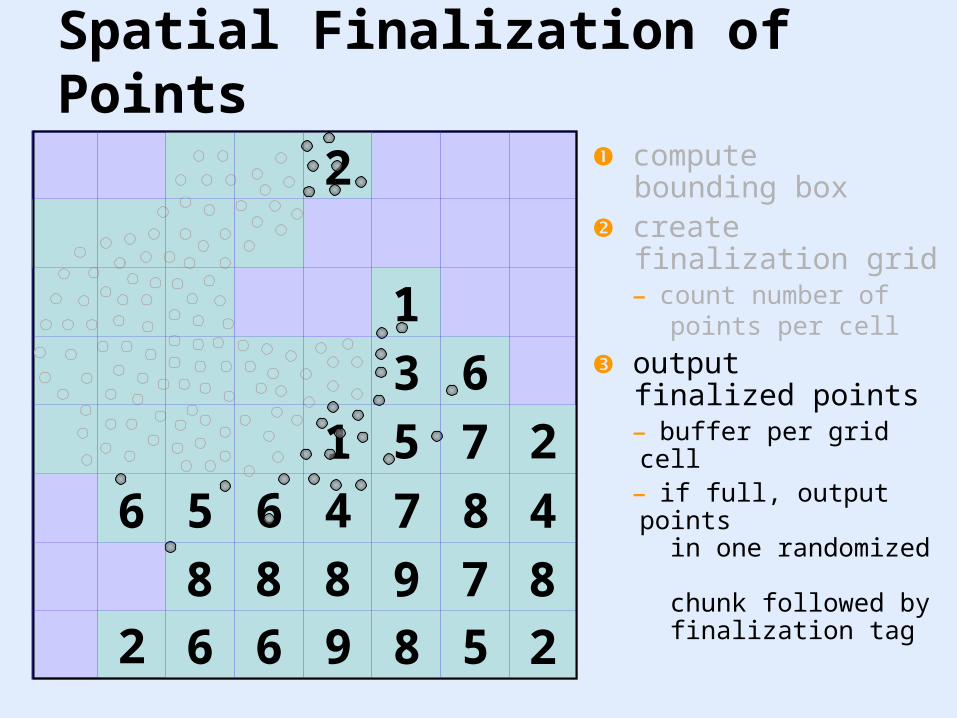
Spatial Finalization of Points
compute bounding box
create finalization grid– count number of points per cell
output finalized points – buffer per grid cell– if full, output points in one randomized
chunk followed by finalization tag
1
7
4
7
9
7
3
4
8
9 7
9 8 5
4
8
2
7
78
86 77
73 97
889
662
7 2
7
3
75 8798
5
60
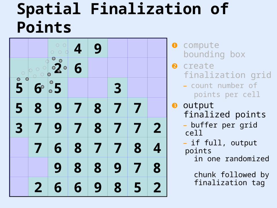
Spatial Finalization of Points
compute bounding box
create finalization grid– count number of points per cell
output finalized points – buffer per grid cell– if full, output points in one randomized
chunk followed by finalization tag
0
2
4
5
9
6
0
4
8
9 7
9 8 5
4
8
2
7
78
86 77
73 97
889
662
7 2
7
3
75 8798
5
61
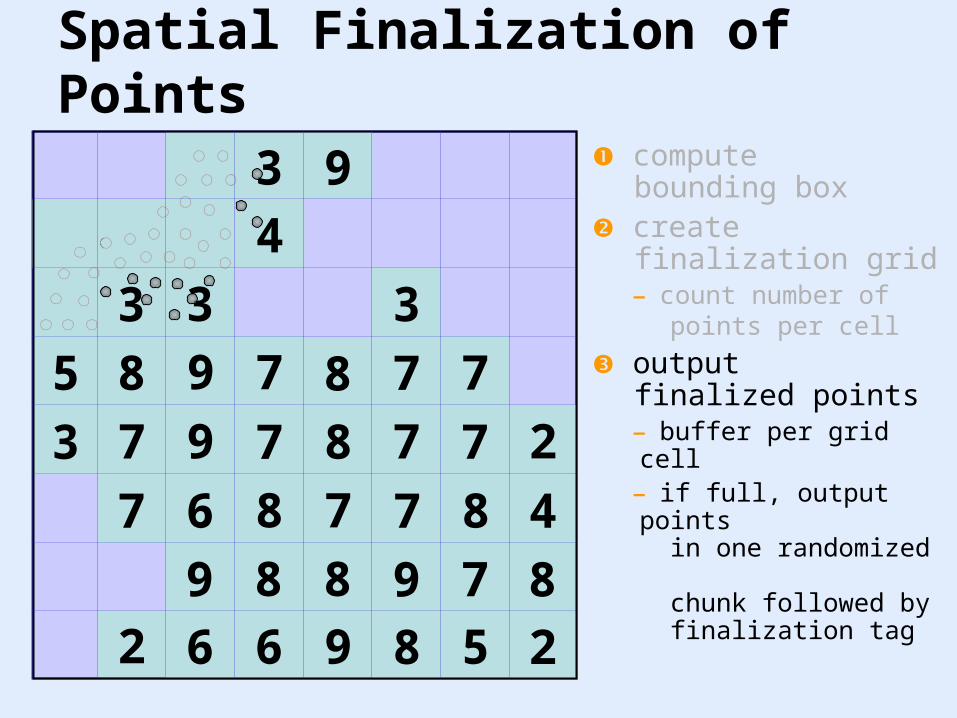
Spatial Finalization of Points
compute bounding box
create finalization grid– count number of points per cell
output finalized points – buffer per grid cell– if full, output points in one randomized
chunk followed by finalization tag
0
0
3
3
9
3
0
4
8
9 7
9 8 5
4
8
2
7
78
86 77
73 97
889
662
7 2
7
3
75 8798
0
41
Spatial Finalization of Points
compute bounding box
create finalization grid– count number of points per cell
output finalized points – buffer per grid cell– if full, output points in one randomized
chunk followed by finalization tag
0 7
0
4
8
9 7
9 8 5
4
8
2
7
78
86 77
73 97
889
662
7 2
7
3
71 7211
1
Spatial Finalization of Points
compute bounding box
create finalization grid– count number of points per cell
output finalized points – buffer per grid cell– if full, output points in one randomized
chunk followed by finalization tag
0 2
0
4
8
9 7
9 8 5
4
8
2
4
51
65 76
888
662
7 2
3
1
6
1
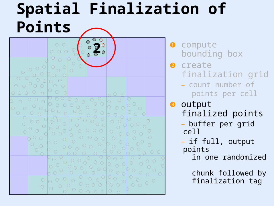
Spatial Finalization of Points
compute bounding box
create finalization grid– count number of points per cell
output finalized points – buffer per grid cell– if full, output points in one randomized
chunk followed by finalization tag

0 2
0
4
3 2
9 7 4
1
7
2
1
233
552
1
Spatial Finalization of Points
compute bounding box
create finalization grid– count number of points per cell
output finalized points – buffer per grid cell– if full, output points in one randomized
chunk followed by finalization tag
0 2
0
4
1
Spatial Finalization of Points
compute bounding box
create finalization grid– count number of points per cell
output finalized points – buffer per grid cell– if full, output points in one randomized
chunk followed by finalization tag
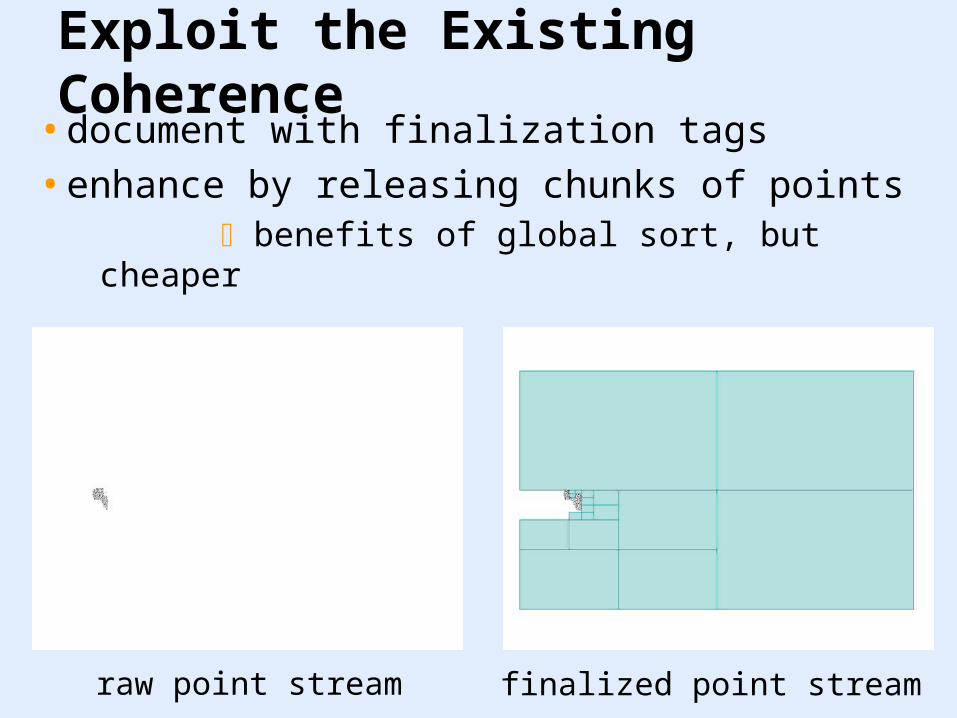
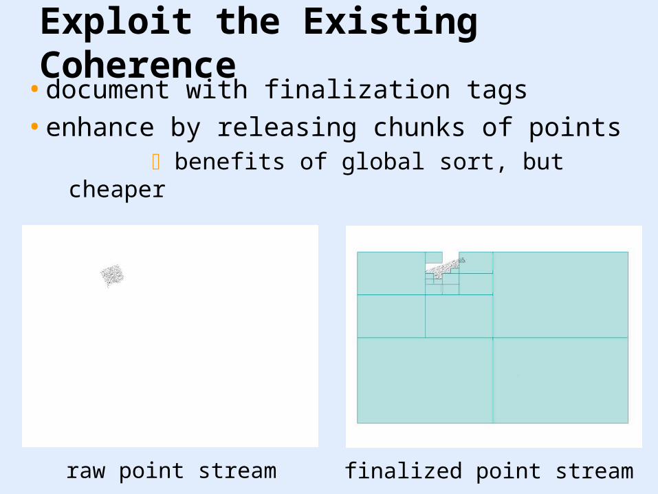
Exploit the Existing Coherence
raw point stream finalized point stream
• document with finalization tags
• enhance by releasing chunks of points benefits of global sort, but cheaper
Exploit the Existing Coherence• document with finalization tags
• enhance by releasing chunks of points benefits of global sort, but cheaper
raw point stream finalized point stream
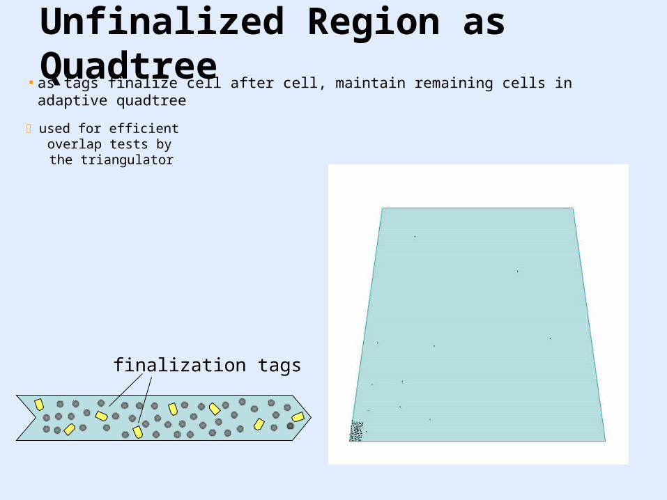
Unfinalized Region as Quadtree• as tags finalize cell after cell, maintain remaining cells in adaptive quadtree
used for efficient overlap tests by the triangulator
finalization tags

The Triangulator
(spdelaunay)
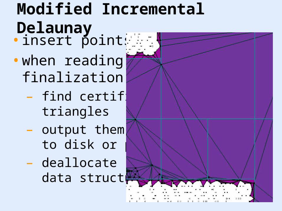
Modified Incremental Delaunay• insert points
• when reading afinalization tag– find certified
triangles
– output them to disk or pipe
– deallocate data structure

Modified Incremental Delaunay• insert points
• when reading afinalization tag– find certified
triangles
– output them to disk or pipe
– deallocate data structure

Modified Incremental Delaunay• insert points
• when reading afinalization tag– find certified
triangles
– output them to disk or pipe
– deallocate data structure
The Rasterizer
(tin2dem)
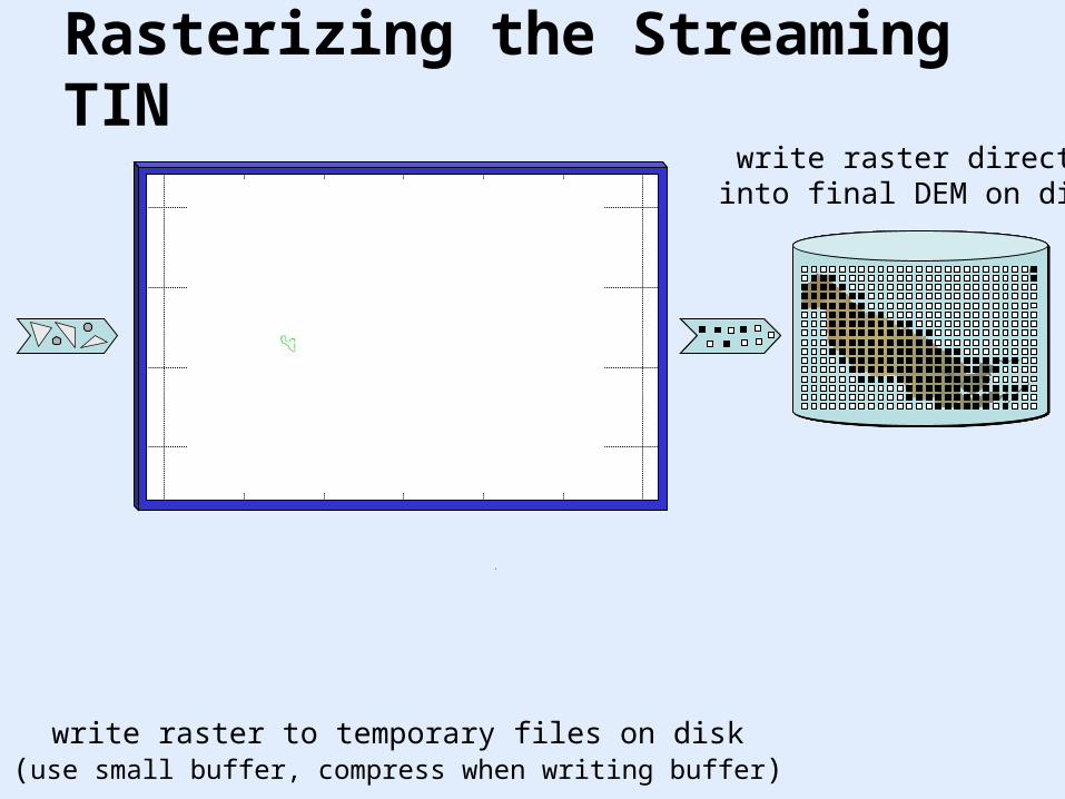
write raster directlyinto final DEM on disk
write raster to temporary files on disk(use small buffer, compress when writing buffer)
Rasterizing the Streaming TIN

Results
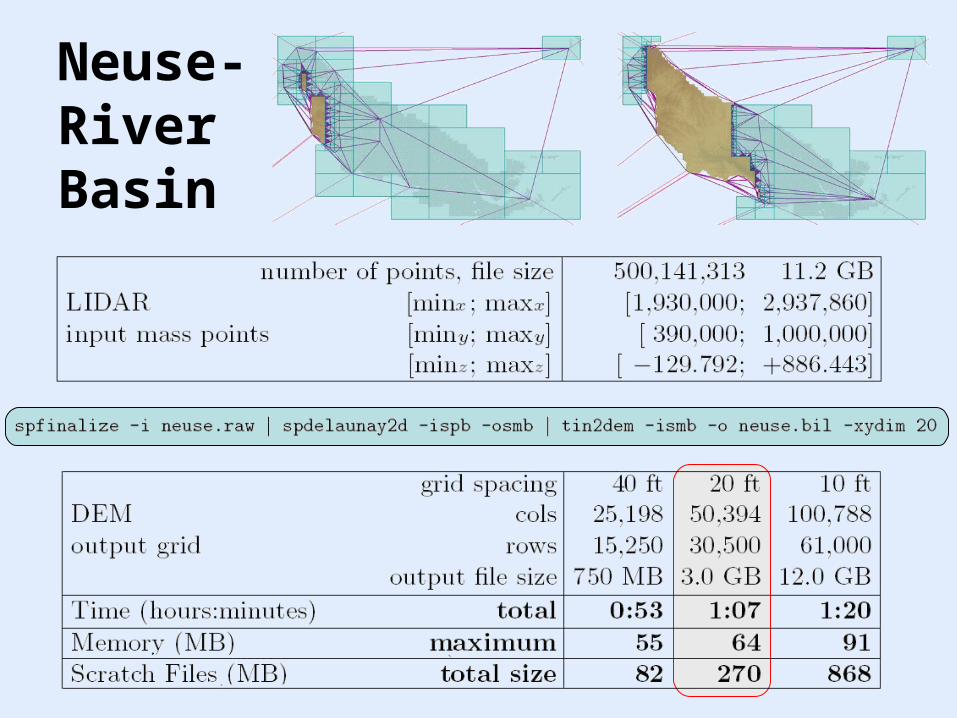
Neuse-RiverBasin

Pipeline Details for the 20 ft DEM
6 min
6 min5 MB
512 x 512 grid
10 MB60,388 triangles
19 MB444 million rasters
43 min 35 MB2,249,268 points
270 MB239 files
8 min
46 MB128 rows per file

• 53 hours– 3.4 GHz desktop
– 10,000 RPM disks
– scratch space:• quadtree: ~ 8 GB
• rasters: ~ 2.5 GB
Comparison to (20 ft)[Agarwal et al. ‘06]
• 67 minutes– 2.1 GHz laptop
– 5,400 RPM disks
– scratch space:• compressed
rasters: 270 MB• 86 % of CPU time for expensive RST– remaining 7.5 hours
• constructing quadtree: 1.1 hours
• finding cell neighbors: 5.6 hours

Demos & Discussion
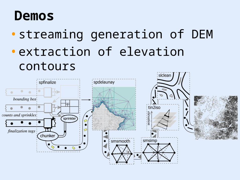
Demos • streaming generation of DEM
• extraction of elevation contours
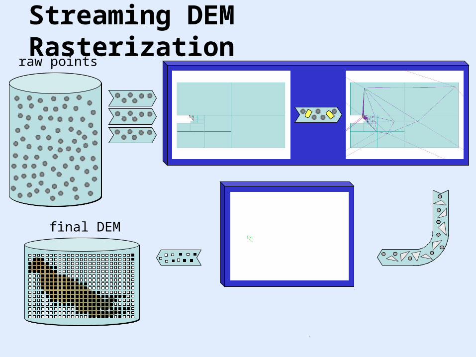
final DEM
Streaming DEM Rasterization raw points

• avoid temporary query structure on disk– data-driven, no gathering of neighbors
Main Features• order of magnitude faster than method
that uses external memory
• no global sort – don’t fight the data, use existing coherence
• interleave input & computation & output– 100% CPU usage while interpolating

• other interpolation methods– natural neighbors
– inverse distance weighting
Future Work• breaklines / barriers (e.g. rivers, roads)
– use Constraint Delaunay Triangulation
• stream other tasks– thinning of points
– compression of raw LIDAR data (useful?)
– hydrological enforcement (streamable?)

Acknowledgements• data
– Kevin Yi, Duke
• support– NSF grants 0429901 + 0430065
"Collaborative Research: Fundamentalsand Algorithms for Streaming Meshes."
– NGA award HM1582-05-2-0003
– Alfred P. Sloan Research Fellowship
Thank You
executables, video, slides, paper, and soon also source code:
http://www.cs.unc.edu/~isenburg/
Top Related