


Languages
Pages
Legal


Frequency-Type Interpretations of Probability
in Bayesian Inferences
July 21, 2017
Contents
1 Introduction 1
2 The Computational Challenge 4
3 Markov Chains Monte Carlo Algorithms 7
3.1 A Metropolis-Hastings Algorithm . . . . . . . . . . . . . . . 10
4 Frequency-Type Interpretations of Probability and MCMC algo-
rithms 13
5 Conclusion 15
1 Introduction
There are many interpretations of probabilities. Following Ian Hacking, we
can say that they fall into two broad categories: belief-type and frequency-
type interpretations. According to the belief-type interpretation, probabil-
1

ities ”are degrees to which someone believes or should believe” (Hacking
2001, p.132). On the other hand, a frenquency-type interpretation implies
that a probability describes a physical property (i.e., a relative frequency, a
propensity, or a disposition).
There is a vast philosophical literature on this topic (See Hajek 2012;
Gillies 2000; Hacking 2001; Eagle 2010) and some have come to believe that
there is no such thing as the correct interpretation:
Each interpretation that we have canvassed seems to capture
some crucial insight into a concept of it, yet falls short of doing
complete justice to this concept. Perhaps the full story about
probability is something of a patchwork, with partially over-
lapping pieces. In that sense, the above interpretations might
be regarded as complementary, although to be sure each may
need some further refinement (Hajek 2012).
In this paper, I aim to provide more support to this claim by pointing
out that we often combine various interpretations of probability when we
make scientific inferences. Of course, links between the two interpretations
have been made in the philosophical literature. They are usually to the
effect that knowing the stochastic properties of a physical system should
influence our degrees of beliefs about that system. Here is a classic exam-
ple:
Knowing the objective probability of getting heads with a par-
ticular coin should, it seems reasonable to believe, also tell you
how likely it is that the next toss of the coin will yield a head.
(Howson and Urbach 2006, p.15-16).
2

But here I want to underscore something totally different. I want to
show that a pluralist account of probability is desirable for its practical ben-
efits. The fact is that a probability density function f (x) that represents our
posterior belief about a parameter of interest within a Bayesian inferential
framework, can be very difficult to compute. Yet, if we give a frequentist
interpretation to that very same density f (x), then we can easily resolve
that computational problem.
In other words, I aim to support a pluralist interpretation of probabil-
ity by pointing out that a frequentist interpretation of probability is very
useful in order to proceed with purely Bayesian inferences. Both interpre-
tations complement each other in practice in a way that has not yet been
addressed by philosophers (tt will thus come as no surprise that I do not
reference many philosophical papers). This absence from the philosophical
literature can perhaps be attributed to a bias towards theoretical concerns
as opposed to the actual computational challenged involved in making sta-
tistical inferences.
This paper is divided into three main parts. In the first part, I will in-
troduce the basics of Bayesian inferences and the computational challenges
that it faces. In the second part, I explain how we can meet those challenges
with Markov Chains Monte Carlo (MCMC) algorithms. In the final part, I
will underscore that such algorithms rest on a frequency-type interpreta-
tion of probability and that they also illustrate the importance of computer
simulations in scientific inferences. They have received very little attention
in philosophy circles and it is time to catch up with the scientific practice.
3
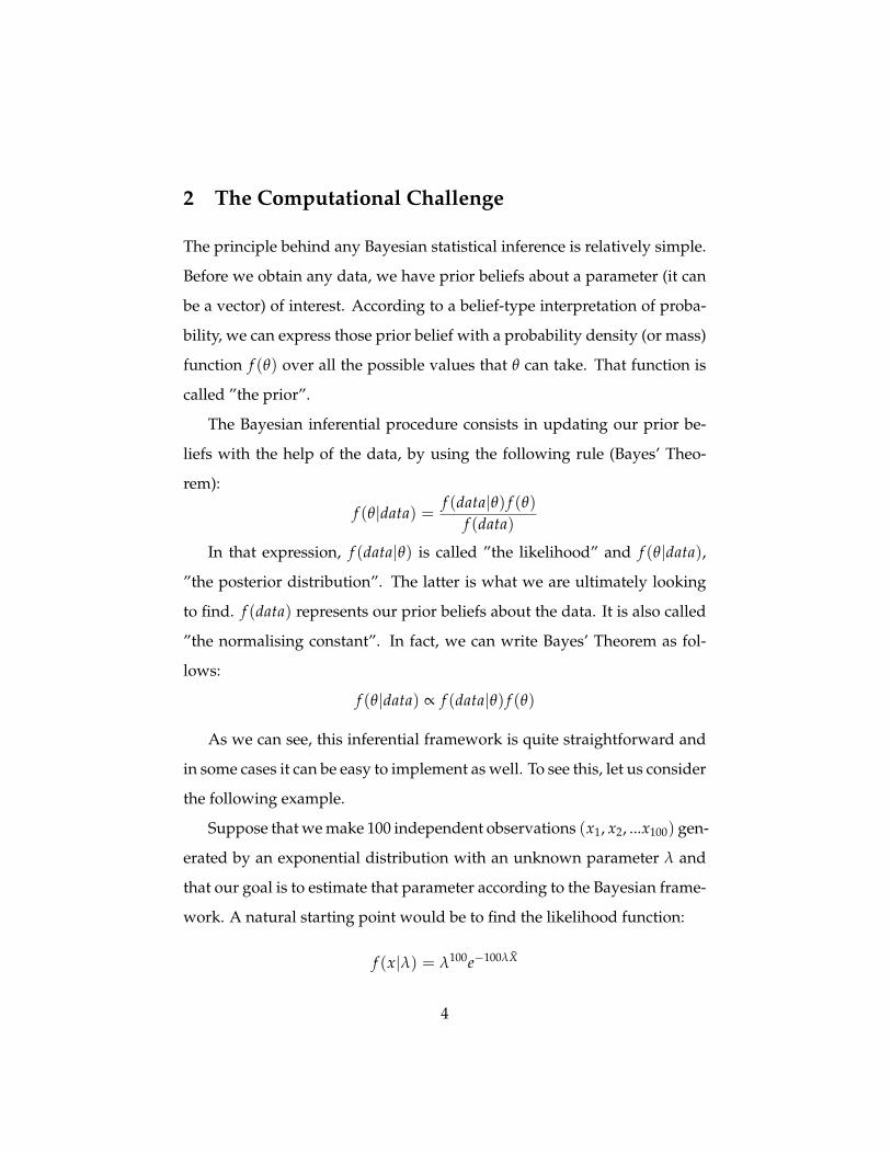
2 The Computational Challenge
The principle behind any Bayesian statistical inference is relatively simple.
Before we obtain any data, we have prior beliefs about a parameter (it can
be a vector) of interest. According to a belief-type interpretation of proba-
bility, we can express those prior belief with a probability density (or mass)
function f (θ) over all the possible values that θ can take. That function is
called ”the prior”.
The Bayesian inferential procedure consists in updating our prior be-
liefs with the help of the data, by using the following rule (Bayes’ Theo-
rem):
f (θ|data) =f (data|θ) f (θ)
f (data)
In that expression, f (data|θ) is called ”the likelihood” and f (θ|data),
”the posterior distribution”. The latter is what we are ultimately looking
to find. f (data) represents our prior beliefs about the data. It is also called
”the normalising constant”. In fact, we can write Bayes’ Theorem as fol-
lows:
f (θ|data) ∝ f (data|θ) f (θ)
As we can see, this inferential framework is quite straightforward and
in some cases it can be easy to implement as well. To see this, let us consider
the following example.
Suppose that we make 100 independent observations (x1, x2, ...x100) gen-
erated by an exponential distribution with an unknown parameter λ and
that our goal is to estimate that parameter according to the Bayesian frame-
work. A natural starting point would be to find the likelihood function:
f (x|λ) = λ100e−100λX̄
4

Next, we might want to choose a gamma distribution for a prior be-
cause it is the conjugate prior to the likelihood of an exponential distri-
bution. This means that the multiplication of a gamma distribution with
the likelihood of an exponential distribution will result in another gamma
distribution - a well known distribution. Conjugate priors are thus partic-
ularly useful because they allow us to determine a familiar posterior dis-
tribution without having to find the normalising constant. In the case at
hand, it implies that we do not need to compute the following integral:∫f (x|λ) f (λ)dλ
Indeed, given Bayes’ Theorem, we know that
f (λ|x) ∝ λ100e−100λX̄λα−1e−λβ
∝ λ(α+100)−1e−λ(100X̄+β)
Thus we can immediately see that the posterior distribution is a gamma
distribution with parameters (α + 100) and (100X̄ + β). In sum, if we wish
to make a Bayesian inference about λ, all we need to do is to specify the
parameters of the conjugate prior distribution (the hyperparameters) that
best correspond to our prior beliefs and simply update the parameters of
that conjugate prior in order to find the posterior distribution.
Unfortunately, we cannot always use this neat trick. It is not applica-
ble in every context. The appropriate posterior function does not always
have a familiar functional form. We thus eventually have to face the bur-
den of solving complex and high dimensional integrals in order to find the
normalising constant or posterior probabilities. In fact, Bayesian statistics
relies heavily on our capacity to integrate complex and high dimensional
5

functions for calculating marginal posterior distributions or posterior ex-
pectations as well (Brooks 1998, p.69).
When an explicit evaluation of those integrals is not possible, then we
need to use algorithms that allow us to make reasonable approximations.
MCMC algorithms are a family of algorithms that are used precisely for
that purpose. ”MCMC has proven to be extremely helpful for such Bayesian
estimates, and MCMC is now extremely widely used in the Bayesian sta-
tistical community” (Roberts et al. 2004, p.22).
According to some, those algorithms actually revolutionised the field of
Bayesian statistics:
Markov chain Monte Carlo (MCMC) techniques [...] have rev-
olutionized the field of Bayesian statistics. Prior to Gelfand
and Smith (1990) demonstrating the applicability of MCMC to
problems of Bayesian inference in 1990, Bayesian statistics had
been a largely academic, and somewhat controversial, pursuit.
Since that time, however, a great many applied scientists, in all
fields of research, have embraced the ideas behind the Bayesian
paradigm (Lunn et al. 2009, p.1).
Markov Chain Monte Carlo (MCMC) methods are probably the
most exciting development in statistics within the last ten years.
The techniques comprising MCMC are extraordinarily general,
and their use has dramatically reshaped the way applied statis-
ticians go about their work. Models long thought to be in the
”too hard” basket are now well within the reach of quantitative
researchers. In short, MCMC constitutes a revolution in statis-
tical practice, with effects just beginning to be felt within the
6

social sciences (Jackman 2000, p.375).
In the next section, I will explain the basic characteristics of such algo-
rithms and give an elementary example of a Metropolis-Hastings MCMC
algorithm. This will allow me to show how frequentist-type interpretation
of probabilities play a crucial role in the application Bayesian inferences in
science.
3 Markov Chains Monte Carlo Algorithms
MCMC algorithms rely on two basic ideas: Monte Carlo integrations and
Markov chains. Monte Carlo methods consist in using repeated random
sampling to estimate certain quantities. Their name is a reference to Monte
Carlo casinos. It was given by a group of scientists working on the Man-
hattan Project.
A Monte Carlo integration of a function is an approximation of the in-
tegration of that function. To use it, we need to follow two simple steps.
Firstly, we need to express the integration that we wish to estimate in the
form of an expected value with respect to a density g(x):
I =∫
f (x)dx =∫ f (x)
g(x)g(x)dx = Eg
[f (x)g(x)
].
Secondly, we use the following estimator for I:
1n
n
∑i=1
f (Xi)
g(Xi)
where (X1, X2, X3, ..., Xn) are independent variables that follow the distri-
bution g(x). The justification for this estimator is that the Strong Law of
7

Large Numbers implies that it will converge almost surely toward I as n
goes to infinity.
When the integral that we wish to estimate is a cumulative distribution
function, which is often the case in Bayesian scenarios, the estimator is even
more straightforward to obtain:
I* =∫ t
∞f (x)dx =
∫ ∞
−∞f (x)1]−∞,t](x)dx = E f [1]−∞,t]]
. Thus we are going to estimate this integral with the empirical cumulative
distribution1n
n
∑i=1
1]−∞,t](xi)
and a sample of independent variables that follow the distribution f (x)
(notice that the expected value here is with respect to f (x)).
In short, Monte Carlo estimators are very useful and they can be used in
a wide variety of contexts. But we need to be able to draw a sample of inde-
pendent and identically distributed variables that follow a specific density
in order to use them and this is not always an easy task. In a Bayesian con-
text for example, we might not even know the normalising constant of the
density that we are trying to integrate. This is where Markov chains come
in handy.
Markov chains describe a stochastic physical process. They describe
the movement of a point in space and in time. With appropriate random
number generators, Markov chains allow us to generate a sample from a
distribution that we want to estimate. With that sample we can use Monte
Carlo estimators and make inferences about the distribution of interest.
To understand this in more details, let Xt stand for the value of a ran-
dom variable at time t. Let t be a natural number (discrete time) and the
8

possible values of Xt, the real numbers (uncountable state space). Finally,
let us define a density K, which is a kernel of transition, such that
P(a < Xt+1 < b|Xt = xt, Xt−1 = xt−1, ..., X0 = x0)
=
P(a < Xt+1 < b|Xt = xt)
=∫ b
aK(Xt+1|Xt = xt)
We have thus defined a Markov chain on an un-countable state space that
can fully describe a random walk on that state space. Such a random walk
can be seen a point (a particle) that moves in time on the real line according
to the kernel of transition. In other words, the value of the variable X can
change at any given time according to K.
If it is possible to transition to any state from any state, then that chain
is said to be irreducible. Moreover, if for any state we can occupy that state
two consecutive times in a row, then that chain is said to be aperiodic and
positively recurrent. If a Markov chain is irreducible, aperiodic, and pos-
itively recurrent, then it has a unique stationary distribution. This means
that as time goes infinity, the sequence of random variables that define the
chain will tend to follow a unique probability distribution p(x).
Now the ”magic” of MCMC algorithms is to create a Markov chain such
that its stationary distribution is precisely the distribution from which we
want to obtain a sample in order to use Monte Carlo integrations. With
enough iteration of that chain, we will indeed obtain the appropriate sam-
9
ple that we need.
In simple terms, this means that if we are trying to compute a probabil-
ity density f (x) that represents a posterior distribution within a Bayesian
framework and that we can create a physical stochastic system such that its
stationary density is precisely f (x), then we can use a Monte Carlo integra-
tion in order to estimate f (x) by sampling many times from the stationary
distribution. Given that the Monte Carlo estimation of the stationary dis-
tribution is easier to find than to compute the posterior distribution, then
we will use the frequentist interpretation of f (x) in order to solve a com-
putational problem that stemmed from a subjective interpretation of f (x).
This interplay of interpretations in order to find convenient computa-
tional solutions to a given problem shows how both interpretations of prob-
ability are intertwined in the scientific practice. It is a vivid example of a
pluralistic interpretation of a concept at play in the scientific practice.
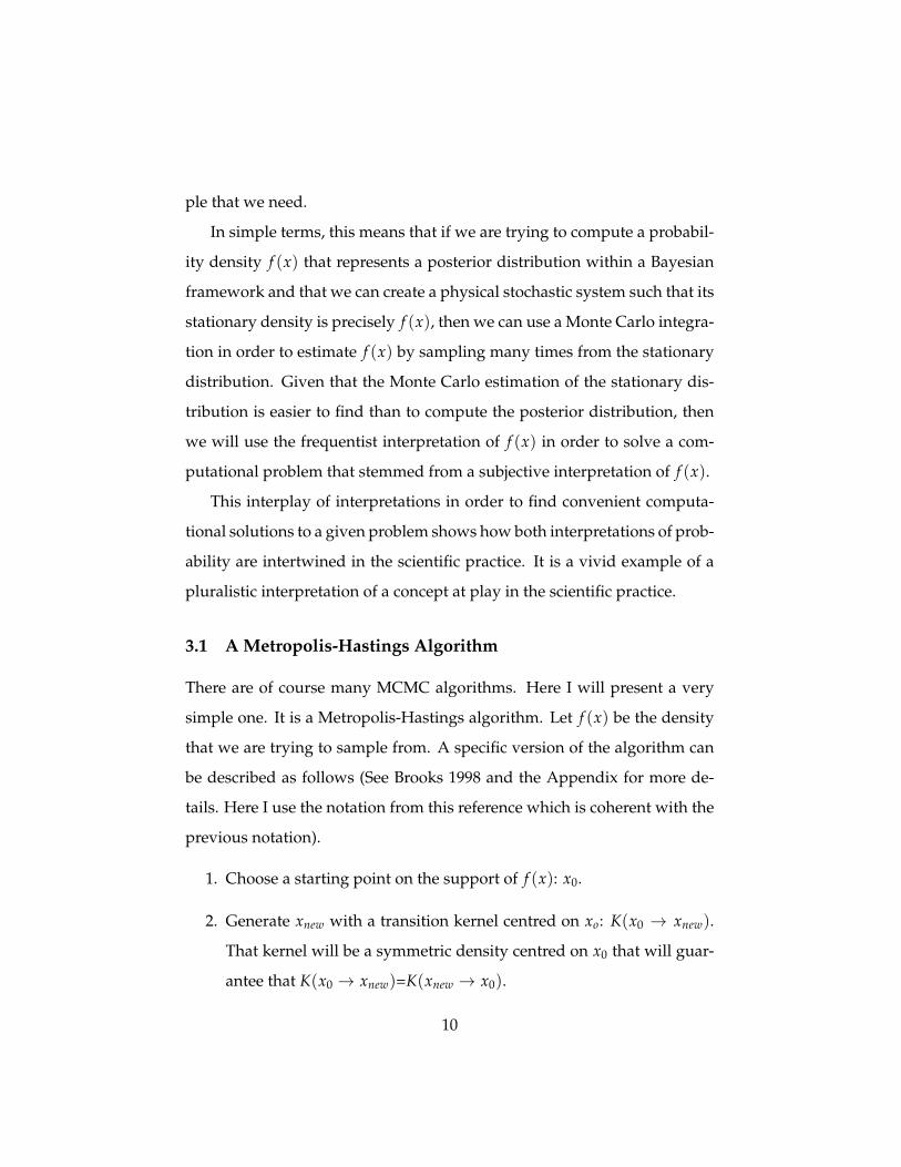
3.1 A Metropolis-Hastings Algorithm
There are of course many MCMC algorithms. Here I will present a very
simple one. It is a Metropolis-Hastings algorithm. Let f (x) be the density
that we are trying to sample from. A specific version of the algorithm can
be described as follows (See Brooks 1998 and the Appendix for more de-
tails. Here I use the notation from this reference which is coherent with the
previous notation).
1. Choose a starting point on the support of f (x): x0.
2. Generate xnew with a transition kernel centred on xo: K(x0 → xnew).
That kernel will be a symmetric density centred on x0 that will guar-
antee that K(x0 → xnew)=K(xnew → x0).
10

3. Compute the probability α of transitioning to the state xnew:
α = min[
1,f (xnew)K(x0 → xnew)
f (x0)K(xnew → x0)
]4. Draw a random number u from a uniform distribution on [0, 1]. If
u < α, then take xnew as the new starting point and start over again.
If not, then stay at xo and start over again.
Notice that the normalisation constant of f (x) will be cancelled by the di-
vision in step 3. So we never need to know it in the first place. Moreover,
we have just created a Markov chain with a unique stationary distribu-
tion. With the appropriate kernel of transition the state space of the Markov
chain will be the support of f (x); it will be possible to access any state from
any state; and it is possible to remain in any state from any state. Also, the
fact that stationary distribution is f (x) is guaranteed by the choice of the
kernel (See Tierney 1994).
To see this algorithm at work in a Bayesian context, let us apply it to the
problem presented in section 2. This will provide a tidy and vivid illustra-
tion. We can also easily make all the computations with the program R (See
the Appendix). Furthermore, we will be able to compare the results with
the true posterior distribution.
For the sake of this example, let us say that λ = 5. With this infor-
mation we will be able to generate a sample of a 100 independent obser-
vations from that exponential distribution and try to estimate λ. Once we
have completed this step, we then define the likelihood function and the
conjugate prior as we did before. We then choose the parameters for the
conjugate prior (the hyperparameters). This choice is determined by our
prior beliefs about λ. Let us agree on β = 0.5 and α = 2. Finally, we com-
pute a Metropolis-Hastings 100 000 times, with a starting value of 1 and a
11

Figure 1: An application of a Metropolis-Hastings algorithm to estimate the pa-
rameter of an exponential distribution
normal kernel of transition of variance equal to 1. It is important to let the
chain run for a long time in order to approximate the stationary distribu-
tion. The resulting random walk z1 can be visualised in Figure 1.
If we make an histogram of the resulting sample, we can see (Figure 2)
that we have a pretty good estimate of the true posterior distribution (rep-
resented in red) for the parameter λ. Even if our sample does not consist
of independent observations, the convergence toward the stationary dis-
tribution allows for the application of Monte Carlo integrations. We can
thus make various inferences about λ by using the empirical cumulative
distribution (See section 3). For example, we can estimate a 95% credibility
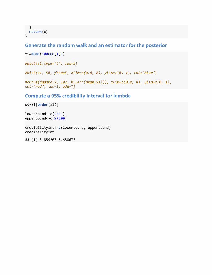
interval for λ (See Appendix):
CI = [3.859203; 5.688675]
12

Figure 2: An historgram estimate of the true posterior distribution (red line)
based on a sample obtained with a MCMC algorithm
This means that the probability that the true value for λ belongs to CI is
0.95.
4 Frequency-Type Interpretations of Probability and
MCMC algorithms
In sum, the goal of the previous algorithm is to estimate an unknown den-
sity that represents our posterior belief about λ. One of the things that we
know about that density is that we can also define it as the stationary den-
sity of a Markov chain. It is the exact same density! In other words, we
know that the density can describe our posterior belief about λ and that it
can also describe the long run behavior of a Markov chain.
13

Knowing about this dual description, we therefore create a physical sys-
tem, a Markov chain, that has the desired long run behavior. Consequently,
we start the simulation and we let it run for a long time. We then compute
appropriate Monte Carlo estimators with the resulting random walk. We fi-
nally end up estimating a density that describes the stationary distribution
of the Markov chain our posterior belief about λ at the same time.
What I want to underscore now is the use of random number genera-
tors in the MCMC algorithm. In order to create a sample from the posterior
distribution (which is also a stationary density), we first had to generate a
random sample that follows the density determined by the kernel of tran-
sition. This is the purpose of the R function ”rnorm” in the code presented
in the Appendix. It is used in order to complete step 2 of the algorithm. We
also had to generate a sample from a uniform distribution in step 4 of the
algorithm. This is why we used the R function ”runif” in the Appendix.
In other words, the validity of the MCMC algorithm and of the underlying
Bayesian inference crucially depended on our capacity to generate num-
bers that follow a very specific probability density (the kernel of transition
or the uniform distribution).
By definition random number generators are described by a frequency-
type interpretation of probability (otherwise they would not be random).
The theoretical foundation of a MCMC algorithms rests on genuine physi-
cal randomness. If the random walk did not objectively display the desired
physical stochastic behaviour of the stationary density, regardelss of our be-
liefs, then we would not be able to produce adequate estimates.
Of course, we only need physical processes that simulate genuine ran-
domness in order to obtain satisfactory results. The R functions that I have
used are only pseudo-random generators. But pseudo-random genera-
14

tors are useful insofar as they can approximate genuine physical random-
ness and genuine physical randomness only makes sense when we use a
frequency-type interpretation of probability.
5 Conclusion
At last, we are in a position to assess the different interpretations of proba-
bility that are at play when we use a MCMC algorithm, like the Metropolis-
Hastings algorithm, in a Bayesian context. Here is the main ”take-away”
argument in a nutshell:
• When a density f (x), representing our posterior beliefs about a parameter is
difficult to compute, we often create a stochastic physical process such that
its stationary density is precisely f (x). By using Monte Carlo integrations
based on samples from that stationary density we can relatively easily esti-
mate f (x). This shows how a frenquency-type interpretation of probability
can be used in some Bayesian inferences because the random walk created
by the Markov chain need to objectively display (or approximate) the desired
physical stochastic behaviour of the stationary density, regardelss of our be-
liefs, in order to produce adequate estimates.
Note that I am not arguing that the resulting Bayesian inferences are ac-
tually a frequentist inferences. I am pointing out that different interpreta-
tions of probability yield different methods to estimate functions such that
the same probability density f (x) can be estimated with more ease if we
use its alternative interpretation. Hence, a pluralist account of probability
is desirable for its practical benefits.
15
Some authors have already mentioned the possibility of a pluralist in-
terpretation of probability. I have argued that it is already implemented in
the scientific practice by shedding light on the importance of MCMC meth-
ods. This was missing from the philosophical literature.
This interplay of interpretation cannot be easily observed through the
usual theoretical study of the notions of probability that we often encounter
in the philosophical literature. It become apparent when we study the prac-
tical challenges of computing certain functions. This is is an aspect of statis-
tical inferences that has been ignored for too long in philosophy of science.
References
Albert, J. (2009). Bayesian computation with R. Springer Science & Business
Media.
Brooks, S. P. (1998). Markov chain monte carlo method and its application.
The statistician, 69–100.
Eagle, A. (2010). Philosophy of probability: contemporary readings. Routledge.
Gelfand, A. E. and A. F. Smith (1990). Sampling-based approaches to
calculating marginal densities. Journal of the American statistical associa-
tion 85(410), 398–409.
Gillies, D. (2000). Philosophical theories of probability. Psychology Press.
Hacking, I. (2001). An introduction to probability and inductive logic. Cam-
bridge University Press.
Hajek, A. (2012). Interpretations of probability. In E. N. Zalta (Ed.), The
Stanford Encyclopedia of Philosophy (Winter 2012 ed.).
16
Howson, C. and P. Urbach (2006). Scientific reasoning: the Bayesian approach.
Open Court Publishing.
Jackman, S. (2000). Estimation and inference via bayesian simulation: An
introduction to markov chain monte carlo. American Journal of Political
Science, 375–404.
Kochanski, G. (2005). Monte carlo simulation. U RL www. ugrad. cs. ubc. ca/˜
cs405/montecarlo. pdf .
Lunn, D. J., N. Best, and J. C. Whittaker (2009). Generic reversible jump
mcmc using graphical models. Statistics and Computing 19(4), 395–408.
Robert, C. and G. Casella (2011). A short history of markov chain monte
carlo: subjective recollections from incomplete data. Statistical Science,
102–115.
Roberts, G. O., J. S. Rosenthal, et al. (2004). General state space markov
chains and mcmc algorithms. Probability Surveys 1, 20–71.
Tierney, L. (1994). Markov chains for exploring posterior distributions. the
Annals of Statistics, 1701–1728.
17

Simple Example
I give a simple example of a MCMC algorithm to estimate the posterior distribution of the parameter (lambda) of an exponential distribution. I use the conjugate prior beta(2, 0.5).
For numerical stability, I use the log of the prior, of the likelihood, and of the posterior. Notice that I do not need to take any constant into account when I construct those functions.
Generate the sample from an exponential distribution (lambda=5)
set.seed(3934) n=100 x1<-rexp(n, 5)
Define the log-prior (conjugate), the log-likelihood, and the log-posterior
logprior<- function(bet, alph, lam){ log(lam)*(alph-1)-(lam*bet) } loglikelihood<-function(lam){ n*log(lam)-lam*n*mean(x1) } logposterior=function(lam){ loglikelihood(lam)+logprior(0.5, 2, lam) }
Define the MCMC algorithm with a normal kernel
MCMC <- function(niter, start, kernelsd){ x<-rep(0,niter) x[1]<-start for(i in 2:niter){ currentx<-x[i-1] proposedx<-rnorm(1,mean=currentx,sd=kernelsd) A<-logposterior(proposedx)-logposterior(currentx) if(log(runif(1))<A){ x[i]<-proposedx } else { x[i]<-currentx }
} return(x) }
Generate the random walk and an estimator for the posterior
z1=MCMC(100000,1,1) #plot(z1,type="l", col=3) #hist(z1, 50, freq=F, xlim=c(0.8, 8), ylim=c(0, 1), col="blue") #curve(dgamma(x, 102, 0.5+n*(mean(x1))), xlim=c(0.8, 8), ylim=c(0, 1), col="red", lwd=3, add=T)
Compute a 95% credibility interval for lambda
o<-z1[order(z1)] lowerbound<-o[2501] upperbound<-o[97500] credibilityint<-c(lowerbound, upperbound) credibilityint
## [1] 3.859203 5.688675
Top Related