


Languages
Pages
Legal


Forecasting Food Price Inflation in Developing Countries with Inflation Targeting Regimes: the Colombian Case
Eliana González Banco de la República
Cra. 7 No. 17-78, Bogotá, Colombia Phone: 571-343-0727
e-mail: [email protected]
Miguel I. Gómez Cornell University 148 Warren Hall
Phone: 607-255-8472 e-mail: [email protected]
Luis F. Melo
Banco de la República Cra. 7 No. 17-78, Bogotá, Colombia
Phone: 571-343-0398 e-mail: [email protected]
José L. Torres
Banco de la República Cra. 7 No. 17-78, Bogotá, Colombia
Phone: 571-343-0125 e-mail: [email protected]

2
Abstract
Many developing countries are adopting inflation targeting regimes to guide monetary policy
decisions. In such countries the share of food in the consumption basket is high and policy
makers often employ total inflation (as opposed to core inflation) to set inflationary targets.
Therefore, central banks need to develop reliable models to forecast food inflation. Our literature
review suggests that little has been done in the construction of models to forecast short-run food
inflation in developing countries. We develop a model to improve short-run food inflation
forecasts in Colombia. The model disaggregates food items according to economic theory and
employs Flexible Least Squares given the presence of structural changes in the inflation series.
We compare the performance of this new model to current models employed by the central bank.
Next, we apply econometric methods to combine forecasts from alternative models and test
whether such combination outperforms individual models. Our results indicate that forecasts can
be improved by classifying food basket items according to unprocessed, processed and food
away from home and by employing forecast combination techniques.
JEL: C22, E31, Q11
Keywords: Food Inflation, Time Series,

3
Forecasting Food Price Inflation in Developing Countries with Inflation Targeting
Regimes: the Colombian Case
Inflation targeting (IT) was first adopted by New Zealand’s central bank in 1990. Since then,
twenty one countries have adopted this regime to formulate monetary policy and others are
expected to follow in the future. According to Pétruson (2004), IT is gaining popularity
worldwide because it sets clear standards to evaluate whether central banks achieve their
inflationary goals, keeps them accountable and guarantees their independence (Kiruhara, 2005).
Various recent evaluations also attest for the success of inflation targeting (Bernanke et al., 1999;
Corbo and Schmidt-Hebbel, 2000; Mishkin, 2003).
Under inflation targeting central banks commit to a target level of inflation, usually over
a one-year horizon. However, there is no agreement regarding which measure of inflation to
target. Some countries employ core inflation (i.e., excluding items such as food and energy
which exhibit high short-run price volatility resulting from external shocks) while others focus
on total consumer price index (CPI). Using total CPI may be more appropriate in developing
countries with inflation targeting regimes for at least two reasons. First, the share of food
expenditures in household budgets in developing countries is much higher than in developed
countries. Second, food prices in developing countries tend to be more volatile than in their
developed counterparts because they have (1) higher prevalence of fresh over processed foods,
(2) lower share of food away from home in total food budget and (3) higher market
imperfections. Consequently the high share of food in household budget as well as its high price
volatility results in substantial impacts on total CPI.

4
We posit that developing countries that are inflation targeters should develop reliable
models to forecast food inflation that can be incorporated into models simulating the
transmission mechanism of monetary policy. Although in general monetary policy should not
respond to temporary supply shocks, as is the case of food inflation, large changes in food prices
may affect inflation expectations and thereby increase the permanence of the shock. Thus, food
inflation is relevant to the monetary authorities because inflation expectations are one of the four
channels through which monetary policy transmits to the economy. Lomax (2005) and Bernanke
(2004) discuss the importance of having reliable forecasts for the formulation of monetary
policy.
In this paper we present a model developed by the Colombian central bank to forecast
short-run food inflation (over one to twelve-month horizon) using monthly data from December
1988 to May 2006. Our model is based on the economic determinants of food prices established
by economic theory and incorporates various applied econometric issues such as: does
decomposing food inflation into its components outperform forecasts of aggregate food
inflation? Do forecasts that use fixed parameters (e.g. ordinary least squares) outperform models
that allow for parameters that change over time (e.g. flexible least squares)? Does combining
predictions obtained from different methodologies improve the forecast of food inflation? Our
work contributes to extant empirical literature because little has been done to systematically
address the links between food prices and monetary policy in the context of inflation targeting.
The paper is organized as follows. In Section 2 we review the literature focusing on the
IT framework, the role of food inflation forecasts within inflation targeting, and earlier models
developed to forecast food inflation. In Section 3 we briefly review the theoretical underpinnings
of our empirical model, we discuss the current strategies employed by the Colombian central

5
bank to forecast food inflation in the short and medium-run, and we point out the need to
improve food inflation forecasts to guide the central model. Section 4 explains our empirical
procedures; Section 5 presents the data used in our analysis; Section 6 discusses our results and
Section 7 concludes and proposes areas for future research.
Literature Review
In this section we describe the IT framework, we discuss the role of short term forecasts within
this framework focusing in particular on food inflation, we review earlier models discussed in
the literature to forecast food inflation, and we state the contribution of our study.
The inflation targeting framework
According to Walsh (2003), a targeting regime is a policy framework in which a central
bank is responsible for achieving a pre-specified objective. Such objective involves a quadratic
loss function measuring the deviation of a variable (or a set of variables) from its pre-specified
target levels. The role of a central bank under a targeting regime is therefore to implement policy
that minimizes the expected discounted value of the loss function. Among targeting regimes, the
most widely adopted by countries around the world is inflation targeting. Inflation targeting
involves the central bank announcing inflationary goals for a time horizon accompanied by an
aggressive strategy to communicate with the public about its monetary plans and objectives
(Bernanke et al. 1999). Economists often refer to inflation targeting as a one-step approach
because inflation rate is the direct object of monetary policy (Kurihara, 2005). This means that
inflation is the key variable in the loss function and is consequently assigned a higher weight
relative to other relevant variables such as output gap or money demand.

6
An IT regime makes explicit the importance of having low long-run inflation as one of
the pillars of sustained economic growth. Kurihara (2005) discusses reasons why many countries
have embraced inflation targeting: (1) it sets clear standards to evaluate whether or not central
banks achieve their inflationary goals and (2) it keeps central banks accountable while
guaranteeing their independence. Bernanke et al. (1999) posit that inflation targeting contributes
to stabilize expected inflation, a key variable in the design of monetary policy. In short, the keys
to success are transparency and credibility (Revankar and Yoshino, 1990).
A number of empirical studies demonstrate the ability of the framework to reduce
inflation in both developed and developing countries (e.g. Almeida and Goodhart, 1998;
Bernanke et al., 1999; Corbo and Schmidt-Hebbel, 2000; Mishkin, 2003). The main conclusion
of these assessments is that inflation targeting has largely been a success. The popularity of
inflation targeting is changing radically the way central banks are setting monetary policy in all
continents to the point that some argue that the framework is setting a new benchmark for the
formulation of monetary policy (Petursson, 2004).
The role of food inflation short-run forecasts in an inflation targeting regime
Under inflation targeting, central banks usually employ two types of models to evaluate
the effects of monetary policy decisions. One type of models focuses on estimating short-run
forecasts (one to twelve-month horizons), assumes constant interest rates (i.e. ignoring the
transmission mechanism of monetary policy), and includes various types of time series models.
The second type consists of a set of recursive equations describing the transmission mechanism
to simulate the impact of monetary policy decision. These models are complementary in the
sense that the short-run forecast models provide initial values for the transmission mechanism
model.

7
There is no consensus regarding whether total inflation or core inflation should be
employed to set inflationary targets. The difference is that core inflation often excludes items in
which prices respond to short-run supply shocks (e.g. food, oil) and items with regulated prices
(e.g. public services). In setting inflationary targets, some countries such as Brazil, Colombia,
Spain, Israel, Mexico, New Zealand, Poland, Sweden and Switzerland use total CPI; and others
such as Canada, Australia, Korea, Iceland and Thailand use core inflation (Debelle, 1997;
Mishlin and Schmidt-Hebbel, 2000; Aboal et al. 2004). The main argument in favor of using
total CPI is that economic agents and the general public create expectations and make decisions
based on total CPI. Moreover, economic agents and the general public are impacted by the whole
basket of consumption, not just by the core items (Minilla et al., 2004). Therefore, setting the
target based on total inflation increases the credibility of the central bank and makes the system
more transparent. On the other hand, proponents of employing core inflation argue total CPI is
influenced by factors beyond the control of the monetary authorities and the need of having a
measure that is less sensitive to temporary price changes and more reflective of the long-term
trends.
Many developing countries using inflation targeting set inflationary goals based on total
CPI. This makes sense for them since generally their share of food in household expenditures is
high and because most of the contracts are indexed to total CPI. Thus, total CPI is more
representative of the loss of the purchasing power of money than any measure of core inflation.1
In developing countries such as Colombia, focusing only on core inflation implies leaving out
food and items with administered prices, which account for about 30 and 10 percent of the
consumption basket, respectively. We note that, in Colombia, inflationary targets are set using

8
total CPI, but monetary policy decisions are based on core inflation, given that the former is
sensitive to short-run exogenous shocks beyond the control of the monetary authority.
Food price inflation models
A challenge for central banks in developing countries setting CPI targets is that their food
inflation tends to have a greater impact on total inflation than in their developed counterparts
because their share of food in household budget is higher and heir food prices tend to be more
volatile. For instance, in Colombia, during the period 1990-2005 food explains about 51 percent
of the CPI variability even though the share of food in total spending is only 30 percent. This
contrasts with an inflation targeting country such as New Zealand, where the share of food
expenditures is 13 percent and the price volatility of food is lower than in developing countries
(Lin, 2003). Given the importance of monitoring food prices in developing countries that have
embraced inflation targeting, a relevant question is: what has been done regarding models to
forecast food inflation? And, do efforts to forecast food inflation play a role in the
macroeconomic models that central banks use to make monetary policy decisions? To address
such questions it is necessary to make a distinction between developed and developing countries.
In developed countries food inflation received considerable attention from the economics
literature during the 1970s and the early 1980s, when food price shocks had substantial impacts
on the national economies (e.g. Lombra and Mehra, 1983). However, interest has decreased in
recent years because of the secular decrease of food in household budgets and because the price
volatility of aggregate food prices have decreased. For instance, the increasing share of food
away from home in total food spending makes that food prices depend more on such variables of
the service sector as real estate and wages. Laflèche (1997) and Bryan, Cecchetti and Wiggins
(1997), find that within the food group, food away from home is one of the least volatile

9
elements in the CPI in both the United States and Canada. Additionally, low volatility of food
prices is the result of technology improvements (e.g., biotechnology and storage).
The case of the United States illustrates uses and estimation methods of food price
inflation in developed countries. The U.S. Department of Agriculture is the only agency that
produces periodic forecasts of food inflation. Such forecasts contribute to define the president’s
annual budget for food and agricultural programs such as the Food Stamp Program (Joutz et al.
2000). Given that the price volatility of food is comparable to non-food inflation, the monetary
authorities do not consider this item in the formulation of macroeconomic models. A survey of
macroeconomic models in inflation targeting countries such as England, New Zealand, Australia,
Norway and Japan leads to the same conclusion: temporary supply shocks related to changes in
food prices are too small to produce policy responses from central banks using inflation
targeting.
Food inflation forecasts produced by the USDA employ a combination of expert
judgment, smoothing techniques and econometric methods. Joutz et al. (2000) conducts a
thorough evaluation of alternative models employed at USDA to forecast food inflation and
compare such models with univariate time-series models for twenty one components of the food
basket. The authors find that not a single method outperforms the others in all periods or models.
For example, univariate time series methods tend to outperform other methods in terms of
smaller RMSEs, but they fail to anticipate changes in trends which are critical in forecasting food
inflation. Consequently, the authors show that the use of techniques to combine predictions
generated by alternative models improves the accuracy of forecasts because they employ a larger
information set.
10
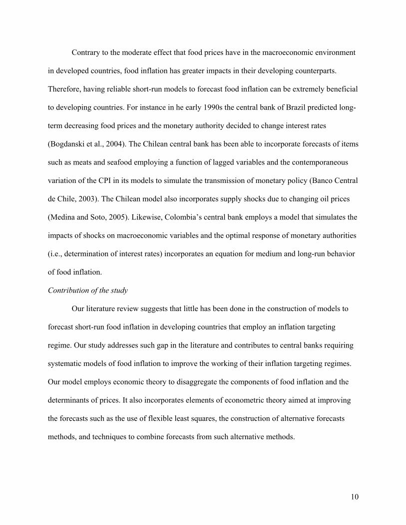
Contrary to the moderate effect that food prices have in the macroeconomic environment
in developed countries, food inflation has greater impacts in their developing counterparts.
Therefore, having reliable short-run models to forecast food inflation can be extremely beneficial
to developing countries. For instance in he early 1990s the central bank of Brazil predicted long-
term decreasing food prices and the monetary authority decided to change interest rates
(Bogdanski et al., 2004). The Chilean central bank has been able to incorporate forecasts of items
such as meats and seafood employing a function of lagged variables and the contemporaneous
variation of the CPI in its models to simulate the transmission of monetary policy (Banco Central
de Chile, 2003). The Chilean model also incorporates supply shocks due to changing oil prices
(Medina and Soto, 2005). Likewise, Colombia’s central bank employs a model that simulates the
impacts of shocks on macroeconomic variables and the optimal response of monetary authorities
(i.e., determination of interest rates) incorporates an equation for medium and long-run behavior
of food inflation.
Contribution of the study
Our literature review suggests that little has been done in the construction of models to
forecast short-run food inflation in developing countries that employ an inflation targeting
regime. Our study addresses such gap in the literature and contributes to central banks requiring
systematic models of food inflation to improve the working of their inflation targeting regimes.
Our model employs economic theory to disaggregate the components of food inflation and the
determinants of prices. It also incorporates elements of econometric theory aimed at improving
the forecasts such as the use of flexible least squares, the construction of alternative forecasts
methods, and techniques to combine forecasts from such alternative methods.

11
The Current Model as a Benchmark
Forecasting at Colombia’s Central Bank has a relative short history. The bank became
independent in 1991 and began announcing inflation targets combined with a crawling band for
the exchange rate as well as controlling the quantity of money. By 1998 the central bank
employed several models to forecast headline inflation and a quarterly Inflation Report was
published. According to Gómez, Uribe and Vargas (2002) these were steps toward a inflation
targeting regime, which the board of directors agreed with three conditions: (1) a true
independence of the central bank, (2) a reasonable ability to predict inflation and (3) a better
understanding of the monetary transmission mechanisms. In 1999 an IT regime was abruptly
forced in Colombia and in other emerging economies due to spillovers from the 1997 Asian
crisis and the 1998 Russian crisis.
In 2001 the central bank started using a transmission mechanisms model to elaborate the
Inflation Report and by that time the board of directors already trusted it to formulate monetary
policy. Most efforts were devoted to improve headline inflation forecasts but events at that time
pointed out the need of models for CPI components. For instance the monetary authority missed
the inflationary target (a total CPI of 6 percent) in 2002 due to an unexpected increase in
potatoes prices and a rapid devaluation in the second semester of that year (total inflation in 2002
was 7 percent but excluding potatoes the total CPI was 6.1 percent). Likewise, in 2003 the
central bank missed the target (5 to6 percent) due to transitory shocks in food supply higher
prices of services. In both years the shocks were unexpected and thereby should not affect in
monetary policy decisions. However, in Colombia a considerable number of prices and contracts
are indexed with the end of year CPI and the credibility of the central bank was at stake. The
bank’s response was twofold: to set targets with a 1% width and to improve forecasting models

12
of food inflation, tradable goods and non-tradable goods. In 2004 a new version of the
transmission mechanism model was implemented taking into account satellite models of tradable
and non-tradable goods as well as food inflation.
Nowadays the staff monitors four different monthly models for food inflation: ARIMA
with exogenous variables (ARIMAX), Group 6, Group 10 and a Neural Network:
1) ARIMAX Model – it forecasts prices for the aggregate food basket using rainfall as a transfer
variable (Based on Avella, 2001).
2) GROUP6 Model (G6) – it divides the food basket into six groups (beef, milk, potato,
vegetables, fruits and all others); uses an error correction model assuming a long-run
relationship between food inflation and non-food inflation; the final forecast is the weighted
average of the six individual forecasts. The model includes as explanatory variables livestock
slaughter, rainfall and an estimation of industrial output gap.
3) GROUP10 Model (G10) – it is similar to GROUP6 model, but divides the food basket into
10 subgroups (meat/eggs, dairy, edible oils, potato, foods away from home, cereals,
tubercles, vegetables, fruits and processed foods); it includes the same explanatory variables
as in GROUP6 model plus the exchange rate with respect to the US dollar and the
international prices of wheat and edible oils.
4) Neural Network Model (NN) – it employs a neural network technique to forecast aggregate
food price inflation from rainfall (measured as the deviation from the average level of rainfall
under normal conditions) and non-food inflation, following the methodology presented in
Torres ( 2006)
However, the forecasting performance of these models has been modest. The average
forecast error including the last 18 months forecasts of the best of these models for one month

13
ahead is 0.44 percent points, but it rapidly increases to 0.64 percent points for forecasts six
months ahead. When the simple average of these four models is considered, the results improve
only slightly. Therefore, the central bank does not consider them very reliable. Moreover, a naïve
model in which forecasts of food inflation are obtained as the weighted difference of the average
forecast for total inflation and non-food inflation outperforms the aforementioned models.
Nevertheless, these models have been useful in determining future trends of food prices and in
predicting the direction of the price changes. We argue that additional efforts are necessary to
improve forecasts of food inflation and that it is possible to improve such forecasts applying
alternative econometric techniques as well as using economic theory. We use the current model
as a benchmark to compare the empirical procedures that we describe in the following section.
Theoretical Underpinnings
The Colombian CPI includes 205 items, of which 59 are food items ranging from salt to fresh
meats to food consumed away from home. Prices of these items do not respond to the same
economic variables, neither follows the same dynamics. However, developing a model to
forecast each individual item may be inefficient because their aggregation incorporates the
forecast errors of each individual forecast. Therefore, it is convenient to employ an intermediate
strategy in which food items are assigned to groups so as to maximize intra-group similarities
and inter-group differences with regard to determinants of their prices. Additionally, it is
necessary to identify key demand and supply variables affecting prices that are readily available
with the frequency required for a monthly forecast model.
We follow the classification used by the U.S. Department of agriculture to forecast food
inflation (Loutz et al., 1997) and decompose the food basket into three main groups: food away

14
from home, processed food and unprocessed food. We argue that the factors determining price
movements across these groups are different. The price formation of food away from home items
relates to the economics of the service sector. That is, salient supply-side factors affecting prices
of these goods include the cost of inputs such as real estate, salaries and public services, among
others. On the other hand, such demand factors as income and demographic characteristics
(Mancino and Kinsey, 2004; Ma et al. 2006) influence food away from home prices, although
they are hard to incorporate in our model because most are fixed in the short-run.
Unprocessed food consists mostly of short-cycle crops and their prices are sensitive to
weather and own lagged prices (Tomek and Robinson, 2003). Other factors affecting planting
decisions in the short-run which impact consumer prices include input prices, expectations of
own prices and those of other commodities competing for the same resources, transportation
costs and credit. The demand for unprocessed foods tends to be price inelastic in the short run
and demand factors are unlikely to yield price volatility. Processed food items belong to the
industrial sector and, as such, the main determinants of prices are the industrial output gap and
the lagged inflation of tradable goods (most items included in processed foods are tradable).
In addition to disaggregating food inflation into its components based on economic
theory, various econometric techniques can contribute to improved forecasts of food inflation. In
particular, we hypothesize that techniques yielding parameter estimates that vary over time such
as flexible least squares (FLS) and applying methods to combine forecasts from different models
should improve the models’ predicting ability. The FLS methodology was first proposed by
Kalaba and Tesfatsion (1989, 1990) and it can be understood as a time-varying linear estimation.
FLS forecasts can capture structural changes and generally outperform forecasts based on
ordinary least squares. Following Kalaba and Tesfatson (1990), let ty be a dependent variable,

15
tX a k dimensional vector of exogenous variables and tb a vector of unknown coefficients. The
methodology is based on two assumptions: that the relationship between ty and tX is
approximately linear at each t (Measurement Relation) and that the vector tb exhibits small
changes over time (Dynamic Relation). In mathematical form,
(1) TtbXy ttt ,,10' L=∀≈− (Measurement Relation)
(2) Ttbb tt ,,101 L=∀≈−+ (Dynamic Relation).
The FLS estimator is defined as ( ) ( )( )2 2arg min ; ; ; 0M Db
r b T r b Tµ µ+ >
where ( ) [ ]2
1
2 ; ∑=
′−=T
ttttM bXyTbr and ( ) [ ] [ ]tt
T
tttD bbbbTbr −′−= +
−
=+∑ 1
1
11
2 ; are the sum of the
measure and dynamic quadratic deviations. The parameterµ captures the weights of the two
deviations on the objective function and it is estimated from the minimization problem. Note that
as µ approaches zero the objective function does not assign weight to the dynamic error. In
contrast, when µ →∞ , the objective function gives most of the weight to the dynamic error.
Thus the function is minimized if 2 0Dr = and the method is equivalent to OLS.
The procedures described above focus on improving forecasts by allowing the parameter
estimates to vary over time. Another way to achieve the same goal is to employ econometric
methods that combine information from various models. Thus, the second econometric technique
that we employ is the optimal combination of individual forecasts. Starting with pioneer work by
Bates and Grander (1969), extant literature shows that combined forecasts often outperform
individual forecasts in terms of smaller mean squared forecast errors (Clemen, 1989 ; Hendry

16
and Clements, 2004, and Elliott and Timmermann, 2004). We focus on combination methods
pertaining to two aspects that are relevant to food inflation in Colombia during the past two
decades: the series are integrated of order one and the occurrence of structural changes (Melo
and Misas, 1998, 2004).
We follow Hallman and Kamstra (1989) and Coulson and Robins (1993) combination
methodologies. Both studies assume that the forecasting series are non-stationary. Since there
may be structural changes during our period of analysis, we modify their methods using a state
space representation in which the intercept of the model follows a random walk process. Thus,
the intercept is allowed to change over time (Melo and Nunez, 2004). Consequently, let tY be the
forecasting series, ihttf −| be the thi forecast model (i=1,…, K), and ),...,,,( 210 ′kγγγγ be a
vector of estimating parameters. Hallman and Kamstra methodology for the h forecast horizon
is based on the following regression,
(3) 1 20 1 | 2 | |. . . k
t h h t t h h t t h k h t t h tY f f fγ γ γ γ ε− − −= + + + + + ,
subject to 1...21 =+++ kγγγ , where ( )2~ 0, 1,2, ,t iid t Tε σ = K . Then, the h-period ahead
forecast combination is given by
(4) 1 2| 0 1 | 2 | |
ˆ ˆ ˆ ˆ ˆ.. . kt h t h h t h t h t h t k h t h tY f f fγ γ γ γ+ + + += + + + + .
On the other hand, Coulson and Robins combination methodology is based on the
following linear model:
(5)
1 20 1 | 2 | |( ) ( ) ... ( )k
t h t h t ht t h h h t t h h t t h kh t t h tY Y f Y f Y f Yγ γ γ γ ε− − −− − − −− = + − + − + + − + ,
where the h-step ahead forecast combination is obtained as

17
(6) 1 2| 0 1 | 2 | |
ˆ ˆ ˆ ˆ ˆ( ) ( ) ... ( )kt h t t h h t h t t h t h t t k h t h t tY Y f Y f Y f Yγ γ γ γ+ + + += + + − + − + + − .
We note that the combined forecast is the weighted average of the individual forecasts
obtained from the individual models. We include an intercept if at least one of the individual
forecasts is biased. Additionally, the Coulson and Robins method equals the Hallman and
Kamstra method when the sum of all weights is restricted to one.
Data and Empirical Procedures
The data consist of monthly food price indexes for the period 12/1989 – 04/2006 for the fifty
nine food items that enter the CPI and the corresponding series of explanatory variables. We
employ the period 12/1989 – 09/2002 for estimation and we produce forecasts for the period
10/2002 – 04/2006. As explained earlier, these fifty-nine items are classified into three sub-
components: processed food, food away from home and unprocessed food (fresh fruits,
vegetables and tubercles), with shares in the food basket of 23, 19 and 58 percent, respectively.
In order to obtain stationary series, we first transform the data by applying logarithms and taking
first and seasonal differences. Then, we estimate a model to forecast the inflation of each of these
groups separately.
In Figure 1 we present the dynamics of total food inflation and its components. The
figure shows that unprocessed food is by far more volatile than the other components and than
the aggregate food inflation. Additionally, the figure suggests that all series exhibit a structural
change in 1999: before 1999, annual food inflation was nearly 20% and after the mid 1999 it
decreased rapidly to a one digit number. Such structural change is the result of several factors,
such as increasing free trade, changes in the structure of the consumption basket and recovery
from El Niño in 1998. We conducted a test of structural change using the ARIMAX model for

18
total food inflation including lags of the dependent variable and lags of precipitation. The test,
developed by Quandt (1960), is based on the F test proposed by Chow 1960)2 but taking the
supreme F-statistic among all possible break points in the series. We note that the critical values
on the Quandt test are not from the standard F distribution but from a non standard distribution
(Andrews, 1993; and Andrews and Ploberger, 1994). Figure 2 exhibits the F-statistics for each
point in time showing a break in the series after mid 1999 at 5% significance level.
[Insert Figure 1 here]
[Insert Figure 2 here]
The processed food inflation model includes lags of the dependent variable, of tradable
goods inflation (i.e. items which prices depend on exchange rate) and of output gap as
explanatory variables. Since processed food and tradable goods are both closely linked to the
behavior of the real exchange rate, we use tradable goods inflation as explanatory variable for the
prices of processed food. We did not include exchange rate, since there is not an accurate
forecast model for this variable. In order to obtain a smooth series, we estimate the output gap by
using the twelve-month moving average of the gap obtained with a Hodrick and Prescott filter
from the monthly industrial production index. In Figure 3 we present further details of the data
used in estimation. Figure 3a presents annual inflation of processed food along with tradable
goods inflation. Figure 3b shows that the deviations of the processed food inflation from the
tradable goods inflation are closely correlated to the output gap.
[Insert Figure 3 here]
The food away from home model incorporates as explanatory variables lags of the
dependent variable and of non-food inflation. In Figure 3c we present the annual inflation of both
series, showing that there is a close relationship between these series. This is mainly because

19
non-food inflation contains all services (e.g., electricity, rent and gas) that affect prices of food
away from home and because wages are correlated to CPI. This relationship is also implied by
the error correction models G6 and G10 that are currently used at the central bank.
The prices of unprocessed food exhibit a cobweb behavior, which is more pronounced in
developing countries where producers have financial restrictions hindering them to behave
against the cobweb cycle. Figure 3d presents the annual unprocessed food inflation, where this
pattern is clear. We employ a two step procedure where we first fitted a basic autoregressive
model to the series of unprocessed food and the unexpected component was calculated as the
residuals from this model. We in turn estimate the unprocessed food model using lags of the
dependent variable and lags of the unexpected estimated component of prices. We note that for
this particular case we work with OLS estimates because the forecasts obtained from the model
estimated by FLS did not outperform those obtained by estimating the model with OLS for
forecast horizons greater than four months. Additionally, the estimated parameter µ (which
measures whether or not the parameters are fixed over time) is large, suggesting that the
parameters do not change too much over time. Consequently, we estimate the model of
unprocessed food using OLS including lags of the dependant variable, a moving average
component and a dummy variable for “El Niño” weather phenomenon as explanatory variables.
We employed other explanatory variables for each food group, including factors that
affect demand and supply for those products such as livestock slaughter, rainfall, soil
temperature, cultivated area and international prices, among others. However, we found two
limitations that prevented us from incorporating such variables. First, for many of those variables
there is not available information up to date and with the periodicity required. Additionally, even
if we had the data, we would have to construct models for those variables so that we can use

20
those forecasts in the respective food group inflation. By doing so the forecasts errors increased
substantially.
The model for the three components of food basket yields:
tttt
tttt
GAPGAPTradProcProcProccProc
εγγβααα
+++∆∆+∆∆+∆∆+∆∆+=∆∆
−−
−−−
31111121
212310122112112
lnlnlnlnln
(7)
1214122112112 lnlnln −−− +++∆∆+∆∆=∆∆ ttttt ninoUnprocUnprocUnproc ηϕηλδδ (8)
tt
ttt
NonfoodAwayAwaycAway
ωγαα
+∆∆+∆∆+∆∆+=∆∆
−
−−
3121
12122112112
lnlnlnln
(9),
where LnProc, LnAway and LnNonfood are the logarithms of processed, food away-from-home
and nonfood CPI, respectively; LnTrad is the logarithm of tradable CPI , GAP is the output gap,
nino is a dummy corresponding to the El Niño phenomenon and η is the noise or unexpected
component of unprocessed food. The models for processed food and food away from home were
estimated with FLS while the model for unprocessed food was estimated by OLS. Next, the total
food CPI is constructed as the weighted average of the three indexes:
tttt UnprocAwayprocTotalfood 19.023.058.0 ++= (10)
The next step is to construct out of sample rolling forecasts from September 2002, from
one to six months ahead. That is, for each month the parameters of the model were re-estimated
after adding one new observation and a new set of forecasts were produced until the last
available observation was added (04/2006). Finally the forecasts for total food inflation were
constructed as the weighted sum of the forecasts from the three components in equation10.
We estimate this model (hereafter G3 model) together with the five models currently in
use by the central bank and described earlier: (1) ARIMAX model of aggregate food inflation;
(2) NN model; (3) G6 model; (4) G10 model; and (5) naïve model defined as the difference
between the forecasts of total CPI and nonfood inflation (hereafter Naïve model). These six

21
models are aggregated using a simple average (a naïve combination) and the econometric
forecast combination techniques as discussed in the empirical model. A comparison of such
aggregation methods would allow us to assess the contribution of econometric combination
techniques to improved forecasts.
Prior to combining individual forecasts, it is necessary to test for unbiasedness of the
individual forecasts (Holden and Peel, 1989). This test allows us to characterize the forecast
errors. In the case that the forecasts are biased then the combination equation must include a
constant term. Combination techniques also assume that there is no forecast encompassing
(Harvey, Leybourne and Newbold, 1998). That is, under the null hypothesis, the forecast
encompassing tests indicate that there is a forecast model that incorporates all the relevant
information contained in the other forecasts models. If the test indicates that there is not a
particular model that encompasses all the others then we proceed to combine the forecasts
following Melo and Nunez (2004). Subsequently we compare the combination forecasts with
those obtained from each of the six individual models and a simple average of them.
Findings
We first evaluate inflation forecasts measured as the twelve month-variation of food CPI. We
compare the forecasts from the new model (namely G3, equations 7-10) with those obtained
from the models currently in use at the central bank. We employ such standard measures of
forecast evaluation as mean forecast error (ME), root mean square forecast error (RMSE), root
mean square percent forecast error (RMSPE) and mean average percent forecast error (MAPE).
We also calculate the U-Theil to assess the performance of each model with respect to a random
walk. Table 1 shows that, based on the aforementioned evaluation measures, for forecast
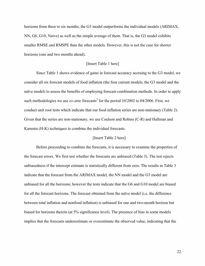
22
horizons from three to six months, the G3 model outperforms the individual models (ARIMAX,
NN, G6, G10, Naive) as well as the simple average of them. That is, the G3 model exhibits
smaller RMSE and RMSPE than the other models. However, this is not the case for shorter
horizons (one and two months ahead).
[Insert Table 1 here]
Since Table 1 shows evidence of gains in forecast accuracy accruing to the G3 model, we
consider all six forecast models of food inflation (the four current models, the G3 model and the
naïve model) to assess the benefits of employing forecast combination methods. In order to apply
such methodologies we use ex-ante forecasts3 for the period 10/2002 to 04/2006. First, we
conduct unit root tests which indicate that our food inflation series are non-stationary (Table 2).
Given that the series are non-stationary, we use Coulson and Robins (C-R) and Hallman and
Kamstra (H-K) techniques to combine the individual forecasts.
[Insert Table 2 here]
Before proceeding to combine the forecasts, it is necessary to examine the properties of
the forecast errors. We first test whether the forecasts are unbiased (Table 3). The test rejects
unbiasedness if the intercept estimate is statistically different from zero. The results in Table 3
indicate that the forecast from the ARIMAX model, the NN model and the G3 model are
unbiased for all the horizons; however the tests indicate that the G6 and G10 model are biased
for all the forecast horizons. The forecast obtained from the naïve model (i.e. the difference
between total inflation and nonfood inflation) is unbiased for one and two-month horizon but
biased for horizons therein (at 5% significance level). The presence of bias in some models
implies that the forecasts underestimate or overestimate the observed value, indicating that the

23
combination procedure must include an intercept in the combination equation in order to obtain
unbiased combination forecasts.
[Insert Table 3 here]
Table 4 shows the results of pair wise encompassing tests, the element located in row i
and column j corresponds to the p-value associated with the null hypothesis that forecasts of the
model i encompass the forecasts of model j. These results show that the G3 model encompasses
the other models for the five and six month forecast horizons. On the other hand, none of the
models encompasses all the others for forecast horizons from one to four months. This indicates
that the combination methodologies would improve the forecast for the first four months but
would not be useful for the five and six forecast horizon.
[Insert Table 4 here]
In Table 5 we show results from the combination techniques. We use the HK and CR
combination methodologies using a state space representation (SS) in which the intercept is
allowed to change over time. We also estimate the HK and CR models by using weigthed least
square method (WLS) which assigns different weights to each period observation, giving more
weight to recent observations. Both methods account for the structural change present in our
food inflation series. In the table we present the combination forecast method with the smaller
RMSE between the HK and the CR techniques, and between SS and WLS estimation methods.
The results allow us to compare the forecast obtained from the combination to the six individual
forecasts of food inflation as well as to the simple average. The main finding is that the
combined forecast outperforms all individual forecasts for all horizons and for all the forecast
errors measures. The only exception is that, for the one month ahead horizon, the MAE and

24
MAPE evaluation measures of the G6 model are smaller than those corresponding to the
combination forecast
[Insert Table 5 here]
We conducted an additional exercise to determine whether forecasting food inflation
from a single model for the aggregated series produces better results than forecasting the sub-
components and then aggregate those forecast to get the total food inflation forecast. We have
three models that estimate the total food inflation (NN, ARIMAX and the naïve model) and three
models where the food basket is divided into groups and the forecast of the total food inflation is
calculated as the aggregation of the components forecasts (G3, G6 and G10). The results in
Table 5 suggest no clear evidence of which strategy produces better forecasts, because not all the
models of one class outperforms the others. Nonetheless, the G3 model is the best in terms of
forecast accuracy (except for one and two-month ahead forecasts). Therefore, choosing between
forecasting aggregate food inflation or forecasting subcomponents and aggregating them depends
on the model, on the classification of items in the food basket and on the estimation
methodology. Our empirical evidence suggests that dividing the aggregate into components is
worth doing inasmuch as not too many groups are considered and these groups must be
heterogeneous among them, and homogeneous within them.
Summarizing our results indicate that the proposed model (G3) as well as the application
of combination techniques tend to yield benefits in terms of more accurate forecasts for some
horizons. The G3 model forecasts tend to encompass the current models for some horizons
indicating that this model contained most of the information of the benchmark and naïve models
in terms of forecasting. Nevertheless, the combined forecasts tend to outperform all individual

25
models for all horizons. We find no evidence to shed light on the issue whether forecasting the
aggregate is better than forecasting the components and then aggregating such forecasts.
Conclusions and Directions for Future Research
The objective of this study was to provide policy makers more reliable short run forecasts
models of food inflation. Our results provides evidence that such forecasts can be improved by
(i) disaggregating food items according to determinants of their prices (processed foods,
unprocessed foods and food away from home) and by (ii) employing econometric methods to
combine forecasts from alternative models. On the other hand, our study does not shed light on
the issue of whether forecasting an aggregate variable (i.e. total food inflation) is preferable than
forecasting its various components and subsequently aggregating such forecasts.
This study is valuable to central banks using an inflation targeting regime in developing
countries in particular because it sheds light on various issues related to the challenges of
producing reliable forecasts of food inflation in the short run. The extreme price variability
exhibited by food items in these countries as well as their large share in total household spending
warrant efforts to construct reliable models of short term food inflation. We hope that our study
attracts the interest of economists in central banks of developing countries so that more research
on the challenging issue of predicting changes in food prices receives more attention for the
literature. We are convinced that such efforts would yield benefits to policy makers in terms of
more appropriate monetary policies.
While we identified strategies to improve food inflation forecasts, we believe there are a
number of possible extensions of our study. First, future research efforts should focus on
developing models using alternative classifications of the food basket. For instance, one aspect to

26
consider is the cyclic behavior of meats and dairy prices, which suggests that one should to
separate them from the processed food group. Additionally, one can consider classifying food as
tradable foods, non tradable foods, food away from home and the cyclic items mentioned earlier
(Jaramillo, et al., 1995). Second, future research should focus on structural models for selected
items with high share in the food basket as well as high price volatility. Examples of such items
include food away from home (by far the fastest growing consumption good in the food basket in
many developing countries), short term crops such as potatoes (given its extreme month-to-
month price variability), meats and dairy, among others. Having these structural models is an
excellent complement of time series models because they can take the role of “expert opinion”
regarding the direction of price changes over longer time horizons (quarter, semi-annual or
annual). Thus, forecasts from the time series models can be adjusted using information from the
structural models.
Second, future research should address the following question discussed in recent
literature (Hendry and Hubrich, 2006): Is forecasting an aggregate variable such as food inflation
better than first forecasting the disaggregate models and then aggregating their forecasts? There
is no consensus in the literature about this issue and efforts to provide an answer could have
important impacts on the models employed by central banks that are inflation targeters. Third,
future research should try alternative econometric techniques such as Neural Networks for each
of the components of food inflation as well as simultaneous estimation of the components using
multivariate methodologies (e.g. prices of food away from home and processed food are affected
by the behavior of unprocessed food prices). Fourth, an interesting empirical question is whether
changing the data frequency from monthly to quarterly improve the forecasts to three, six, nine
and twelve-month horizons. It is possible that monthly data may be better to predict food price

27
changes in the very short run (defined as one to three-month horizon), but quarterly data may be
more appropriate to forecast between three and twelve months. Finally, data availability and
opportunity are an important constraint to econometric modeling in developing countries. Central
banks should make an effort to systematically (and timely) compile secondary data that are
relevant to food inflation forecasts.

28
References
Avella, R. 2001. “Efecto de las Sequias Sobre la Inflación en Colombia.” Borradores de
Economía No. 183, Banco de la República.
Bates, J., and C. Granger.1969. “The Combination of Forecasts,” Operational Research
Quarterly, 20: 451–468.
Bernanke, B.S., T. Laubach, F.S. Mishkin and A.S. Posen. 1999. Inflation Targeting: Lessons
from the International Experience. Princeton: Princeton University Press.
Bernanke, B.S. 2004. “The Logic of Monetary Policy.” Remarks by Governor Ben S. Bernanke
Before the National Economists Club, Washington, D.C. December 2, 2004.
Bogdanski, J., P. Springer de Freitas, I. Goldfajn, and A.A. Tombini. 2001. “Inflation Targeting
in Brazil: Shocks, Backward-looking Prices and IMF Conditionality.” Working Paper,
Series No. 24, Central Bank of Brazil, Sao Paulo.
Bryan M.F., S.G. Cecchetti, and R.L. Wiggins.1997. “Efficient Inflation Estimation.” Working
Paper No. 6183, National Bureau of Economic Research.
Chow, G.C. (1960). “Tests of Equality Between Sets of Coefficients in Two Linear
Regressions”. Econometrica, 28:3, pp 591-605.
Clemen, R.T.1989. “Combining Forecasts: A Review and an Annotated Bibliography.”
International Journal of Forecasting, 5: 559–583.
Coulson, N. and R. Robins.1993. “Forecast Combination in a Dynamic Setting.” Journal of
Forecasting, 12: 63-67.
Elliott, G., and A. Timmermann. 2004. “Optimal Forecast Combinations under General Loss
Functions and Forecast Error Distributions.” Journal of Econometrics, 122: 47–79.
29
Fraga, A., I. Goldfajn, and A. Minilla. 2003. “Inflation Targeting in Emerging Market
Economies.” NBER Working Paper No. 10019, National Bureau of Economic Research,
Inc,.
Gómez, J., J.D. Uribe, and H. Vargas. 2002. “The Implementation of Inflation Targeting in
Colombia.” Borradores semanales de economía No. 202, Banco de la República.
Hallman, J., and M. Kamstra. 1989. “Combining Algorithms Based on Robust Estimation
Techniques and Co-integrating Restrictions.” Journal of Forecasting, 8: 189-198.
Harvey, D., S. Leybourne, and P. Newbold. 1998. “Tests for Forecast Encompassing.”
Journal of Business and Economic Statistics. 16: 254-259.
Hendry, D.F., and M.P. Clements. 2004. “Pooling of Forecasts.” Econometrics Journal, 7: 1–31.
Hendry, D.F., and K. Hubrich. 2006. “Forecasting Economic Aggregates by Disaggregates.”
Discussion Paper No. 5485, Centre for Economic Policy Research.
Jaramillo, C. F., and Jaramillo, P. 1995. “Estructura del Indices de Precios al Consumidor:
Agunas Implicaciones para el Análisis de Inflación”. Borradores de Economía No 39.
Banco de la República.
Joutz, F.L. 1997. “Forecasting CPI Prices: An Assessment.” American Journal of Agricultural
Economics, 79: 1681-1685.
Holden, K. and D.A. Peel.1989. “Unbiasedness, Efficiency and the Combination of
Economic Forecast.” Journal of Forecasting, 8: 175-188.
Kalaba, R., and L. Tesfatsion. 1989. “Time-Varying Linear Regression via Flexible Least
Squares” Computers Math Applied, 17: 1215-1244.
Kalaba, R., and L. Tesfatsion.1990. “Flexible Least Squares for Approximately Linear Systems.”
IEEE Transactions on Systems, Man and Cybernetics, 20: 978-989.

30
Kurihara, Y. 2005. “Why do EU countries use inflation targeting?” Global Business and
Economics Review, 7: 74-84.
Laflèche, T. 1997. “Statistical Measures of Trend Rate of Inflation.” Bank of Canada Review,
Autumn: 29-47.
Lomax, R. 2005. “Inflation Targeting in Practice: Models, Forecasts and Hunches.” Bank of
England Quarterly Bulletin, 45: 237-246.
Lombra, R.E., and Y.P. Mehra.1983. “Aggregate Demand, Food Prices, and the Underlying Rate
of Inflation.” Journal of Macroeconomics 5: 383-98.
Ma, H., J. Huang, F. Fuller, and S. Rozelle. 2006. “Getting Rich and Eating Out: Consumption of
Food Away from Home in Urban China.” Canadian Journal of Agricultural Economics 54:
101-19.
Melo, L.F., and Misas, M.1998. “Análisis del Comportamiento de la Inflación Trimestral en
Colombia Bajo Cambios de Régimen: Una Evidencia a Través del Modelo Switching de
Hamilton.” Borradores semanales de economía No. 86, Banco de la República.
Melo, L.F., and Misas, M. 2004. “Modelos Estructurales de Inflación en Colombia: Estimación
a través de Mínimos Cuadrados Flexibles.” Borradores de Economía No. 283, Banco de la
República.
Melo, L.F., and Núñez H. 2004. “Combinación de Pronósticos para la Inflación en Presencia de
Cambios Estructurales”. Borradores de Economía No. 286, Banco de la República.
Juan Pablo Medina Claudio Soto. 2005. “Oil Shocks and Monetary Policy in an Estimated DSGE
Model for a Small Open Economy.” Working Paper No. 353, Central Bank of

31
Minella, A., P.S. de Freitas, I. Goldfajn, M.K. Muinhos. 2003. “Inflation Targeting in Brazil:
Constructing Credibility under Exchange Rate Volatility.” Journal of International Money
and Finance 22: 1015-1040.
Mishkin, F.S. 2004. “Can Inflation Targeting Work in Emerging Market Countries?” NBER
Working Paper No. 10646, National Bureau of Economic Research, Inc,.
Mishkin, F.S. 2000. “Inflation Targeting in Emerging Market Countries.” American Economic
Review, 90: 105-109.
Pétursson, T.G. 2005. “The effects of inflation targeting on macroeconomic performance.”
Working Papers No. 23, Central Bank of Iceland.
Quandt, R. (1960). “Tests of the Hypothesis That a Linear Regression SystemObeys Two
Separate Regimes.” Journal of the American Statistical Association 55, pp 324-330.
Revankar, N.S., and N. Yoshino. 1990 “An 'Expanded Equation' Approach to Weak-Exogeneity
Tests in Structural Systems and A Monetary Application." Review of Economics and
Statistics, 71: 173-177.
Stone, A., T. Wheatley, L. Wilkinson. 2005. “A Small Model of the Australian
Macroeconomy: An Update.” Research Discussion Paper, Economic Research Department,
Reserve Bank of Australia.
Tomek, W.G., and K.L. Robinson. 2003. Agricultural Product Prices, Fourth Edition, Ithaca:
Cornell University Press.
Torres, J,L. 2006. “Modelos para la Inflación Básica de Bienes Transables y No Transables en
Colombia”. Borradores de Economía No. 365, Banco de la República.
32
Urbanchuk, J.M. 1997. “Commodity Markets, Farm-Retail Spreads, and Macroeconomic
Condition Assumptions in Food Price Forecasting.” American Journal of Agricultural
Economics, 79: 1677-1680.
Walsh, C.E. 2003. Monetary Theory and Policy, Second Edition, MIT Press, Cambridge.
Young II, R.E., L. Wilcox, B. Willott, G. Adams, D.S. Brown. 1997. “Consumer Food Prices
from the Ground up.” American Journal of Agricultural Economics, 79: 1673-1676.

33
Figure 1: Food Inflation and its components
-30.00-20.00-10.00
0.0010.0020.0030.0040.0050.0060.00
Jan-
90
Jan-
91
Jan-
92
Jan-
93
Jan-
94
Jan-
95
Jan-
96
Jan-
97
Jan-
98
Jan-
99
Jan-
00
Jan-
01
Jan-
02
Jan-
03
Jan-
04
Jan-
05
Jan-
06
Food Inflation Processed food food away from home unprocessed fo

34
Figure 2: F Test for structural change of total food inflation

35
Figure 3: Dependent variables, 1990 – 2006
Figure 3a Figure 3b
Processed Food Annual Inflation and Tradable Goods Annual Inflation
0%
5%
10%
15%
20%
25%
30%
35%
40%
Abr-90
Abr-91
Abr-92
Abr-93
Abr-94
Abr-95
Abr-96
Abr-97
Abr-98
Abr-99
Abr-00
Abr-01
Abr-02
Abr-03
Abr-04
Abr-05
Abr-06
processed tradables
Processed Food Annual Inflation Minus Tradable Goods Annual Inflation and the Output Gap
-10%
-8%
-6%
-4%
-2%
0%
2%
4%
6%
8%
Abr-94
Abr-95
Abr-96
Abr-97
Abr-98
Abr-99
Abr-00
Abr-01
Abr-02
Abr-03
Abr-04
Abr-05
Abr-06
(processed - tradables) gap
Figure 3c Figure 3d
Annual Food Out of Home Inflation and Non-Food Inflation
0%
5%
10%
15%
20%
25%
30%
35%
40%
Abr-90
Abr-91
Abr-92
Abr-93
Abr-94
Abr-95
Abr-96
Abr-97
Abr-98
Abr-99
Abr-00
Abr-01
Abr-02
Abr-03
Abr-04
Abr-05
Abr-06
FOH Non-Food
Annual Primary Food Inflation
-30%
-20%
-10%
0%
10%
20%
30%
40%
50%
60%
Abr-90
Abr-91
Abr-92
Abr-93
Abr-94
Abr-95
Abr-96
Abr-97
Abr-98
Abr-99
Abr-00
Abr-01
Abr-02
Abr-03
Abr-04
Abr-05
Abr-06
Primary

36
Table 1: Forecast Evaluation (out-sample of 18 months)
Horizon Model ME RMSE RMSPE MAE MAPE U-THEIL1 month G6 -0.120 0.340 0.061 0.257 0.045 0.7301 month Naïve -0.044 0.406 0.067 0.329 0.054 0.8681 month G3 -0.052 0.452 0.075 0.373 0.062 0.9731 month NN -0.090 0.495 0.083 0.375 0.063 1.0641 month G10 -0.337 0.534 0.093 0.422 0.072 1.1481 month ARIMAX -0.061 0.590 0.099 0.468 0.079 1.269
Horizon Model ME RMSE RMSPE MAE MAPE U-THEIL2 months Naïve -0.149 0.715 0.113 0.598 0.097 0.9912 months G3 -0.129 0.768 0.121 0.589 0.095 1.0682 months G6 -0.412 0.718 0.126 0.617 0.106 0.9982 months NN -0.225 0.782 0.128 0.592 0.098 1.0872 months ARIMAX -0.158 1.002 0.156 0.785 0.127 1.3932 months G10 -0.693 1.000 0.170 0.844 0.143 1.390
Horizon Model ME RMSE RMSPE MAE MAPE U-THEIL3 months G3 -0.184 0.844 0.134 0.672 0.109 0.9403 months Naïve -0.273 0.871 0.143 0.717 0.119 0.9683 months ARIMAX -0.156 1.079 0.168 0.763 0.123 1.2013 months NN -0.402 1.050 0.180 0.789 0.134 1.1693 months G6 -0.708 1.049 0.180 0.908 0.154 1.1673 months G10 -1.074 1.400 0.233 1.241 0.207 1.558
Horizon Model ME RMSE RMSPE MAE MAPE U-THEIL4 months G3 -0.285 0.861 0.141 0.720 0.119 0.8574 months Naïve -0.446 0.933 0.154 0.835 0.138 0.9264 months ARIMAX -0.188 1.062 0.170 0.717 0.117 1.0584 months NN -0.723 1.210 0.207 0.995 0.167 1.2044 months G6 -1.066 1.369 0.228 1.285 0.215 1.3634 months G10 -1.325 1.588 0.261 1.448 0.240 1.581
Horizon Model ME RMSE RMSPE MAE MAPE U-THEIL5 months G3 -0.276 0.987 0.155 0.803 0.130 0.9595 months Naïve -0.517 0.997 0.156 0.891 0.142 0.8335 months ARIMAX -0.187 1.161 0.188 0.950 0.156 0.9725 months NN -0.717 1.147 0.196 0.973 0.164 0.9605 months G6 -1.308 1.476 0.250 1.379 0.231 1.2365 months G10 -1.523 1.757 0.293 1.643 0.273 1.471
Horizon Model ME RMSE RMSPE MAE MAPE U-THEIL6 months G3 -0.371 1.049 0.164 0.783 0.126 0.9366 months Naïve -0.711 1.121 0.175 0.931 0.148 0.8826 months NN -0.640 1.097 0.188 0.900 0.152 0.8646 months ARIMAX -0.295 1.234 0.200 1.104 0.181 0.9726 months G6 -1.403 1.597 0.269 1.455 0.242 1.2586 months G10 -1.571 1.869 0.316 1.693 0.283 1.472

37
Table 2: Unit Root Test for total food CPI
H0: Totalfoodt has unit root
t-Statistic Prob.*
-1,507383 0.5204Test critical values: 1% level -3,592462
5% level -2,93140410% level -2,603944
t-Statistic-1,291753
Test critical values: 1% level -2,6198515% level -1,94868610% level -1,612036
Augmented Dickey-Fuller test statistic
Elliott-Rothenberg-Stock DF-GLS test statistic
Table 3: Unbiasedness test
Horizon ARIMAX NN G6 G10 G3 Naïve1 Month MEAN -0.37 -1.11 -2.57 -3.69 -0.25 -1.40
P-VALUE 0.35 0.14 0.01 0.00 0.40 0.092 Months MEAN -0.25 -1.02 -4.03 -3.70 -0.13 -1.23
P-VALUE 0.40 0.16 0.00 0.00 0.45 0.113 Months MEAN -0.10 -0.72 -6.13 -4.25 0.09 -1.77
P-VALUE 0.46 0.24 0.00 0.00 0.47 0.044 Months MEAN -0.07 -0.30 -7.42 -5.00 0.28 -2.14
P-VALUE 0.47 0.38 0.00 0.00 0.39 0.025 Months MEAN -0.13 0.24 -8.43 -5.23 0.47 -2.54
P-VALUE 0.45 0.41 0.00 0.00 0.32 0.016 Months MEAN -0.47 0.63 -7.31 -4.66 0.29 -2.80
P-VALUE 0.32 0.27 0.00 0.00 0.39 0.00
0 : 0t tY Hα η α= + =

38
Table 4: Encompassing test
H0: Model i emcompasses model j
Horizon 1 Model j
Model i ARIMAX NN Naïve G6 G10 G3ARIMAX 0.000 0.004 0.002 0.002 0.003 0.001
NN 0.078 0.000 0.008 0.025 0.015 0.005Naïve 0.871 0.104 0.000 0.033 0.261 0.022
G6 0.054 0.093 0.057 0.000 0.133 0.033G10 0.024 0.003 0.002 0.029 0.000 0.001G3 0.988 0.185 0.121 0.016 0.112 0.000
Horizon 2 Model j
Model i ARIMAX NN Naïve G6 G10 G3ARIMAX 0.000 0.011 0.008 0.011 0.006 0.008
NN 0.089 0.000 0.023 0.030 0.029 0.006Naïve 0.966 0.045 0.000 0.037 0.055 0.074
G6 0.072 0.030 0.052 0.000 0.190 0.022G10 0.083 0.010 0.011 0.030 0.000 0.004G3 0.987 0.086 0.256 0.015 0.062 0.000
Horizon 3 Model j
Model i ARIMAX NN Naïve G6 G10 G3ARIMAX 0.000 0.024 0.020 0.033 0.020 0.019
NN 0.037 0.000 0.021 0.023 0.033 0.010Naïve 0.915 0.030 0.000 0.103 0.143 0.032
G6 0.021 0.010 0.007 0.000 0.255 0.007G10 0.038 0.020 0.017 0.024 0.000 0.012G3 0.942 0.129 0.183 0.041 0.099 0.000
Horizon 4 Model j
Model i ARIMAX NN Naïve G6 G10 G3ARIMAX 0.000 0.041 0.026 0.040 0.026 0.029
NN 0.008 0.000 0.022 0.039 0.044 0.007Naïve 0.847 0.059 0.000 0.093 0.203 0.065
G6 0.032 0.030 0.018 0.000 0.251 0.011G10 0.043 0.053 0.034 0.020 0.000 0.035G3 0.733 0.084 0.212 0.078 0.105 0.000
Horizon 5 Model j
Model i ARIMAX NN Naïve G6 G10 G3ARIMAX 0.000 0.048 0.045 0.049 0.037 0.040
NN 0.035 0.000 0.039 0.069 0.077 0.024Naïve 0.752 0.103 0.000 0.045 0.343 0.139
G6 0.042 0.041 0.023 0.000 0.357 0.014G10 0.038 0.072 0.033 0.029 0.000 0.045G3 0.440 0.105 0.202 0.102 0.135 0.000
Horizon 6 Model j
Model i ARIMAX NN Naïve G6 G10 G3ARIMAX 0.000 0.033 0.055 0.068 0.052 0.051
NN 0.027 0.000 0.047 0.077 0.080 0.040Naïve 0.613 0.119 0.000 0.162 0.795 0.138
G6 0.042 0.037 0.019 0.000 0.445 0.014G10 0.045 0.074 0.027 0.035 0.000 0.044G3 0.319 0.221 0.208 0.148 0.233 0.000

39
Table 5: Forecast Evaluation (out-sample 18 forecast)
Horizon Model ME RMSE RMSPE MAE MAPE U-THEIL1 month Combination -0.075 0.337 0.058 0.314 0.053 0.7261 month G6 -0.120 0.340 0.061 0.257 0.045 0.7301 month Naïve -0.044 0.406 0.067 0.329 0.054 0.8681 month simple average -0.152 0.406 0.069 0.312 0.053 0.8721 month G3 -0.052 0.452 0.075 0.373 0.062 0.9731 month NN -0.090 0.495 0.083 0.375 0.063 1.0641 month G10 -0.337 0.534 0.093 0.422 0.072 1.1481 month ARIMAX -0.061 0.590 0.099 0.468 0.079 1.269
Horizon Model ME RMSE RMSPE MAE MAPE U-THEIL2 months Combination 0.015 0.527 0.089 0.404 0.068 0.7192 months Naïve -0.149 0.715 0.113 0.598 0.097 0.9912 months simple average -0.372 0.724 0.118 0.597 0.099 1.0062 months G3 -0.129 0.768 0.121 0.589 0.095 1.0682 months G6 -0.412 0.718 0.126 0.617 0.106 0.9982 months NN -0.225 0.782 0.128 0.592 0.098 1.0872 months ARIMAX -0.158 1.002 0.156 0.785 0.127 1.3932 months G10 -0.693 1.000 0.170 0.844 0.143 1.390
Horizon Model ME RMSE RMSPE MAE MAPE U-THEIL3 months Combination 0.167 0.545 0.091 0.458 0.077 0.6473 months G3 -0.184 0.844 0.134 0.672 0.109 0.9403 months Naïve -0.273 0.871 0.143 0.717 0.119 0.9683 months simple average -0.585 0.912 0.149 0.692 0.115 1.0153 months ARIMAX -0.156 1.079 0.168 0.763 0.123 1.2013 months NN -0.402 1.050 0.180 0.789 0.134 1.1693 months G6 -0.708 1.049 0.180 0.908 0.154 1.1673 months G10 -1.074 1.400 0.233 1.241 0.207 1.558
Horizon Model ME RMSE RMSPE MAE MAPE U-THEIL4 months Combination 0.299 0.491 0.082 0.401 0.067 0.5074 months G3 -0.285 0.861 0.141 0.720 0.119 0.8574 months Naïve -0.446 0.933 0.154 0.835 0.138 0.9264 months ARIMAX -0.188 1.062 0.170 0.717 0.117 1.0584 months simple average -0.826 1.046 0.171 0.883 0.145 1.0414 months NN -0.723 1.210 0.207 0.995 0.167 1.2044 months G6 -1.066 1.369 0.228 1.285 0.215 1.3634 months G10 -1.325 1.588 0.261 1.448 0.240 1.581
Horizon Model ME RMSE RMSPE MAE MAPE U-THEIL5 months Combination 0.459 0.604 0.101 0.547 0.091 0.6155 months G3 -0.276 0.987 0.155 0.803 0.130 0.9595 months Naïve -0.517 0.997 0.156 0.891 0.142 0.8335 months simple average -0.934 1.086 0.177 0.957 0.156 0.9095 months ARIMAX -0.187 1.161 0.188 0.950 0.156 0.9725 months NN -0.717 1.147 0.196 0.973 0.164 0.9605 months G6 -1.308 1.476 0.250 1.379 0.231 1.2365 months G10 -1.523 1.757 0.293 1.643 0.273 1.471
Horizon Model ME RMSE RMSPE MAE MAPE U-THEIL6 months Combination 0.471 0.612 0.098 0.523 0.085 0.6446 months G3 -0.371 1.049 0.164 0.783 0.126 0.9366 months Naïve -0.711 1.121 0.175 0.931 0.148 0.8826 months simple average -0.977 1.123 0.185 1.042 0.172 0.8856 months NN -0.640 1.097 0.188 0.900 0.152 0.8646 months ARIMAX -0.295 1.234 0.200 1.104 0.181 0.9726 months G6 -1.403 1.597 0.269 1.455 0.242 1.2586 months G10 -1.571 1.869 0.316 1.693 0.283 1.472
40
Endnotes
1 On this regard a reporter from a major Colombian newspaper once commented “For those who
don’t eat or need transportation, the recent hike in inflation is not a problem” making fun of
comments from a member of the board of directors regarding core inflation stability.
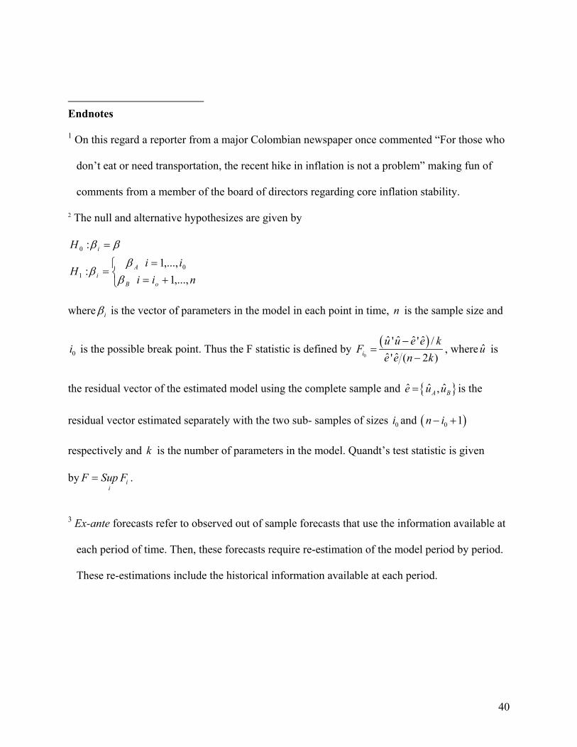
2 The null and alternative hypothesizes are given by
+==
=
=
niiii
H
H
oB
Ai
i
,...,1,...,1
:
:
01
0
ββ
β
ββ
where iβ is the vector of parameters in the model in each point in time, n is the sample size and
0i is the possible break point. Thus the F statistic is defined by ( )0
ˆ ˆ ˆ ˆ' ' /ˆ ˆ' ( 2 )i
u u e e kF
e e n k−
=−
, where u is
the residual vector of the estimated model using the complete sample and { }ˆ ˆ ˆ,A Be u u= is the
residual vector estimated separately with the two sub- samples of sizes 0i and ( )0 1n i− +
respectively and k is the number of parameters in the model. Quandt’s test statistic is given
by ii
F Sup F= .
3 Ex-ante forecasts refer to observed out of sample forecasts that use the information available at
each period of time. Then, these forecasts require re-estimation of the model period by period.
These re-estimations include the historical information available at each period.
Top Related