


Languages
Pages
Legal

ESPOO 2007 VTT WORKING PAPERS 66
0 2 4 6 8 100
1
2
3
4
5
Time (min)
Sm
oke
laye
r h
eig
ht
(m)
Image analysis
Experimental
FDS 20 cm grid
FDS 10 cm grid
0 10 20 300
20
40
60
80
100
120
Time (min)
Tem
per
atu
re (
°C)
)
Meas. E1Meas. E2FDS 20 cm gridFDS 10 cm grid
0 10 20 300
20
40
60
80
100
120
Time (min)
Tem
per
atu
re (
°C)
)
Meas. E1Meas. E2FDS 20 cm gridFDS 10 cm grid
0 5 10 15 20 25 300
50
100
150
200
250
300
350
400
Time (min)
CO
(p
pm
)
FDS 10 cm grid
Measured
FDS 20 cm grid
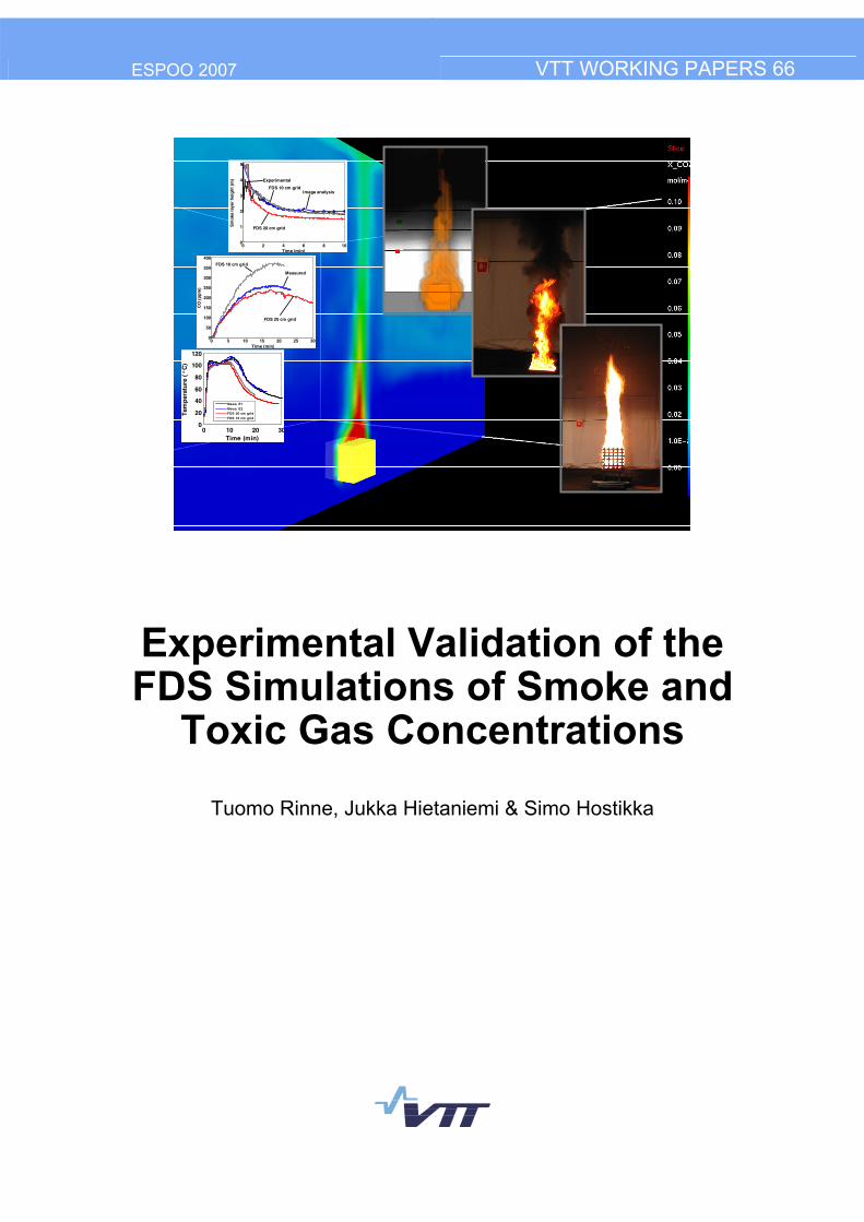
Experimental Validation of the FDS Simulations of Smoke and
Toxic Gas Concentrations
Tuomo Rinne, Jukka Hietaniemi & Simo Hostikka

ISBN 978-951-38-6617-4 (URL: http://www.vtt.fi/publications/index.jsp) ISSN 1459-7683 (URL: http://www.vtt.fi/publications/index.jsp Copyright © VTT 2007
JULKAISIJA � UTGIVARE � PUBLISHER
VTT, Vuorimiehentie 3, PL 1000, 02044 VTT puh. vaihde 020 722 111, faksi 020 722 4374
VTT, Bergsmansvägen 3, PB 1000, 02044 VTT tel. växel 020 722 111, fax 020 722 4374
VTT Technical Research Centre of Finland, Vuorimiehentie 3, P.O.Box 1000, FI-02044 VTT, Finland phone internat. +358 20 722 111, fax +358 20 722 4374
VTT, Betonimiehenkuja 5, PL 1000, 02044 VTT puh. vaihde 020 722 111, faksi 020 722 7027, 020 722 7066
VTT, Betongblandargränden 5, PB 1000, 02044 VTT tel. växel 020 722 111, fax 020 722 7027, 020 722 7066
VTT Technical Research Centre of Finland, Betonimiehenkuja 5, P.O. Box 1000, FI-02044 VTT, Finland phone internat. +358 20 722 111, fax +358 20 722 7027, +358 20 722 7066
Technical editing Anni Kääriäinen
3
Published by
Series title, number and report code of publication
VTT Working Papers 66 VTT�WORK�66
Author(s) Rinne, Tuomo, Hietaniemi, Jukka & Hostikka, Simo Title Experimental Validation of the FDS Simulations of Smoke and Toxic Gas Concentrations Abstract This publication presents an experimental validation of FDS simulations of PMMA, wood, heptane, and toluene fires in a test compartment. The numerical predictions of smoke and gases (CO, CO2 and O2) concentrations, vertical temperature profile, smoke layer height, and visibility are compared against experimental results. Simulations and visualizations were done using FDS and Smokeview version 4.0.5. The results showed that the simulations of CO2 and O2 concentrations and vertical temperature profiles were in good agreement with the measurements. The agreement of the CO concentrations was better in case of toluene and heptane than in case of PMMA and wood. In case of gas concentrations, strong dependency on the grid cell size was observed. For heptane and toluene fuels, the use of default values of Smokeview and FDS leads to good predictions of the view inside a fire compartment. For solid fuels (wood and PMMA) producing smoke that is more gray in colour, the necessary adjustments of the Gray Level visualization parameter are given in order to match the visualizations and video images of the exit sign obscuration. ISBN 978-951-38-6617-4 (URL: http://www.vtt.fi/publications/index.jsp)
Series title and ISSN VTT Working Papers 1459�7683 (URL: http://www.vtt.fi/publications/index.jsp)
Date Language Pages January 2007 English 37 p. + app. 9 p.
Name of project Commissioned by Tekes, the Finnish Funding Agency for
Technology and Innovation and VTT Technical Research Centre of Finland
Keywords Publisher chemical fires, emissions, toxic gases, smoke, simulation, PMMA, wood, heptane, toluene, experimental validation
VTT P.O. Box 1000, FI-02044 VTT, Finland Phone internat. +358 20 722 4404 Fax +358 20 722 4374

4
Preface The work has been carried out in the Fire Research group of VTT Technical Research Centre of Finland. It forms a part of a larger research project launched to develop new tools for fire simulation with the aim set at producing generally acceptable and valid science based tools to meet the needs of fire safety design and risk assessment within the industry and other stakeholders.
The project is funded by Tekes, the Finnish Funding Agency for Technology and Innovation and VTT Technical Research Centre of Finland.

5
Contents
Preface ...............................................................................................................................4
1. Introduction..................................................................................................................6
2. Experimental set up......................................................................................................7 2.1 Test compartment ...............................................................................................7 2.2 Fuels ...................................................................................................................7 2.3 Equipment for measurements and visual monitoring.........................................9
3. FDS simulations.........................................................................................................12
4. Data reduction............................................................................................................14 4.1 Determination of the smoke layer height .........................................................14 4.2 Factors characterising visibility in a smoky environment................................15
4.2.1 Extinction coefficient ...........................................................................15 4.2.2 Visibility...............................................................................................17
4.3 Determination of the visibility and the mean extinction coefficient from the experimental data .............................................................................................17 4.3.1 Method to determine the visibility .......................................................17 4.3.2 Methods to calculate the mean extinction coefficient of FDS and
experiments ..........................................................................................18
5. Results........................................................................................................................20 5.1 Heat release rates..............................................................................................20 5.2 Temperatures ....................................................................................................20 5.3 Gas concentrations............................................................................................26 5.4 Smoke layer height ...........................................................................................28 5.5 Soot density ......................................................................................................31 5.6 Visibility and mean extinction coefficient .......................................................32
6. Summary ....................................................................................................................35
Acknowledgements .........................................................................................................36
References .......................................................................................................................37
Appendices Appendix A: Data files of the FDS simulations Appendix B: Temperature distributions of the experiments
6
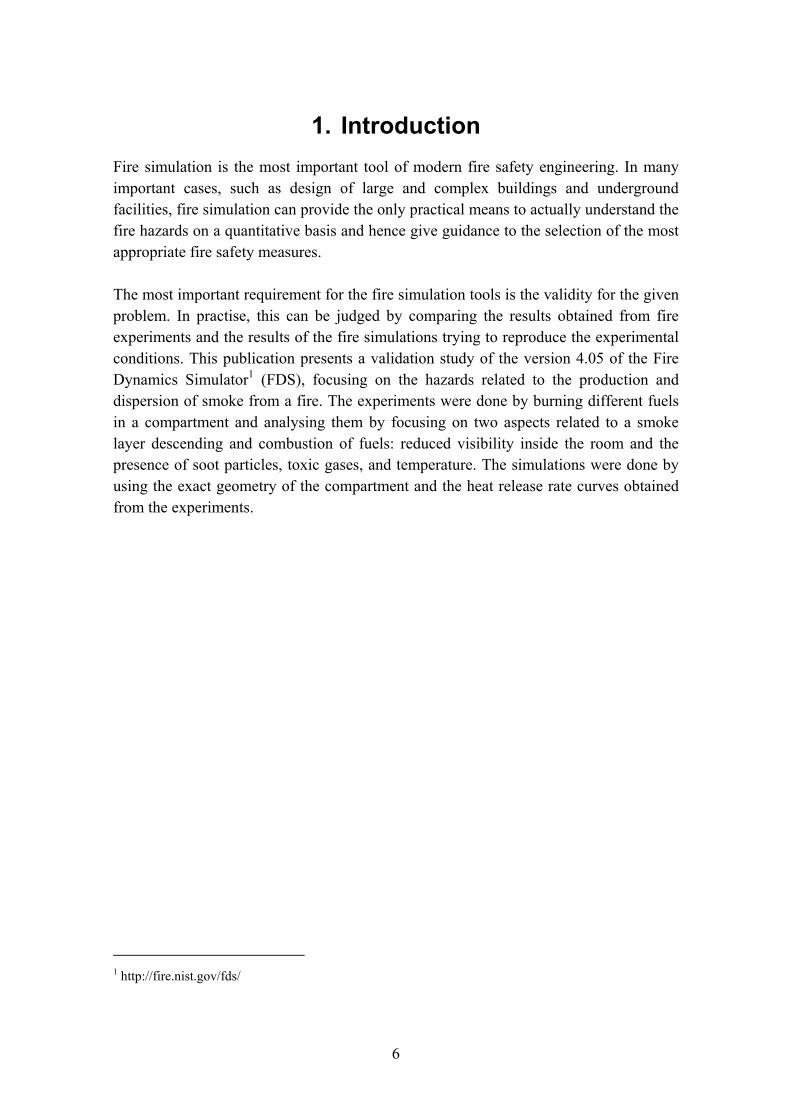
1. Introduction Fire simulation is the most important tool of modern fire safety engineering. In many important cases, such as design of large and complex buildings and underground facilities, fire simulation can provide the only practical means to actually understand the fire hazards on a quantitative basis and hence give guidance to the selection of the most appropriate fire safety measures.
The most important requirement for the fire simulation tools is the validity for the given problem. In practise, this can be judged by comparing the results obtained from fire experiments and the results of the fire simulations trying to reproduce the experimental conditions. This publication presents a validation study of the version 4.05 of the Fire Dynamics Simulator1 (FDS), focusing on the hazards related to the production and dispersion of smoke from a fire. The experiments were done by burning different fuels in a compartment and analysing them by focusing on two aspects related to a smoke layer descending and combustion of fuels: reduced visibility inside the room and the presence of soot particles, toxic gases, and temperature. The simulations were done by using the exact geometry of the compartment and the heat release rate curves obtained from the experiments.
1 http://fire.nist.gov/fds/

7
2. Experimental set up
2.1 Test compartment
The experiments were performed in a 500 m3 compartment, built inside the large fire-test facility of VTT. Figure 1 shows the test compartment lay out and dimensions. The walls of the test compartment were made of 2 mm thick steel with fibreglass insulation. Ceiling material was 2 mm thick steel without the insulation and the floor of the compartment was made of concrete. One ventilation opening of size 2 m × 2 m was left open during the experiments.
Vent 10 m
10 m
5 m2 m
2 m
0.5 m
Vent 10 m
10 m
5 m2 m
2 m
0.5 m
Figure 1. Test compartment used in the experiments.
2.2 Fuels
Four different fuels were used in the experiments. The fuels were selected on the basis of their form and smoke yield. The solid fuels were polymethyl-methacrylate (PMMA) and wood, and the liquid fuels were heptane and toluene. Table 1 shows the properties of the fuels. The experiments began with the first wood crib (notation �E1� in this study) continued with PMMA crib, heptane, toluene, and finally ended with the second wood crib (notation �E2� in this study). The construction of the PMMA and wood cribs are shown in Figures 2 and 3, respectively.

8
Table 1. The fuel properties.
Fuel Heat of
combustion (MJ/kg) a
Soot yield a (kg/kg)
HRRmax (kW)
Fuel geometry
Total mass b
wood c 17.9 0.015 E1: 622.6 E2: 658.8
wood crib (see Fig. 3)
wood: 20.7 kg, heptane: 0.3 kg d
PMMA 25.2 0.022 114.9
PMMA crib inside a
0.25 m2 pool (see Fig. 2)
PMMA: 5.4 kg, heptane: 0.3 kg d
heptane 44.6 0.037 144.7 0.1 m2 pool 4.9 kg toluene 39.7 0.178 149.9 0.1 m2 pool 4.1 kg
a Ref. Tewarson (2002). b Mass loss within 30 minutes except toluene. c Wood crib was used in two experiments. d Heptane was used to ignite the cribs.
Heptane
20 mm
360 mm
30 mm30 mm 30 mm30 mm
Figure 2. PMMA crib construction.
30 3039 100
560
500
30 3039 100
560
500 Figure 3. Wood crib construction. Length of the crib was 500 mm. Units are in mm.

9
2.3 Equipment for measurements and visual monitoring
The experiments were instrumented to measure • concentration of oxygen, carbon dioxide and carbon monoxide • fuel mass loss • gas temperatures • soot density.
Figure 4 shows the locations of the measurement devices.
The gas sampling probe was located inside the compartment at the height of 3.5 m. The gas samples were analysed using two analysers, one for carbon monoxide and carbon dioxide (Siemens, Ultramat 23) and the other for oxygen (Hartmann & Braun AG, Magnos 4G).
Fuel mass was determined by a continuous measurement using a data logging system (Mettler-Toledo AG, Mettler ID1 MultiRange and BalanceLink Ver 2.0). The mass loss rate (MLR) obtained by numerical differentiation of the mass data was used to estimate to heat release rate (HRR) by multiplying the MLR with the heat of combustion of the fuel, given in Table 1.
Temperatures were measured with two thermocouple trees inside the compartment. In each tree there were nine K-type thermocouples (0.5 mm in diameter) between heights 0.5 m�4.5 m above the floor (see Figure 4).
Local soot density was measured using an optical light transmission measurement system (MIREX). The wavelength range of the MIREX is 800�950 nm and the length of the optical path is 2 m. Smoke density measuring was at the height of 3.5 m.
Vent
Fire + mass loss
TCT1
TCT2 MIREX
2.5 m
2.5 m
10 m
10 m
Gas
Ceiling
Floor
0.5 m
thermocouple
Figure 4. Measuring units inside the test compartment (top view on the left). �TCT� stands for thermocouple tree. Side view of the thermocouple tree on the right.
10
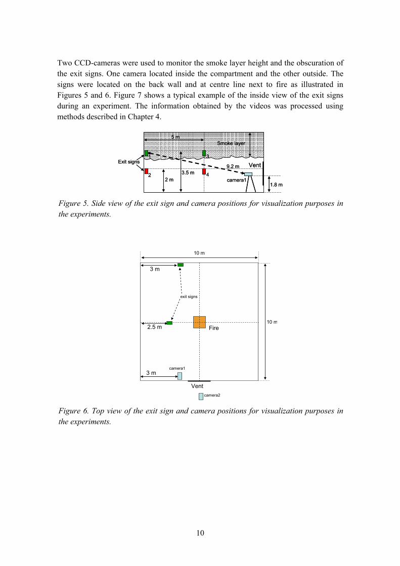
Two CCD-cameras were used to monitor the smoke layer height and the obscuration of the exit signs. One camera located inside the compartment and the other outside. The signs were located on the back wall and at centre line next to fire as illustrated in Figures 5 and 6. Figure 7 shows a typical example of the inside view of the exit signs during an experiment. The information obtained by the videos was processed using methods described in Chapter 4.
camera1
Exit signs
2 m3.5 m
Smoke layer
Vent
5 m
1
2
3
4
1.8 m
9.2 m
camera1
Exit signs
2 m3.5 m
Smoke layer
Vent
5 m
1
2
3
4
1.8 m
9.2 m
Figure 5. Side view of the exit sign and camera positions for visualization purposes in the experiments.
Vent
Fire10 m
10 m
3 m
2.5 m
camera1
exit signs
3 m
camera2 Figure 6. Top view of the exit sign and camera positions for visualization purposes in the experiments.

11
Smoke layer
Exit sign 1
Exit sign 2
Exit sign 4
Exit sign 3
z = 3 m
z = 2 m
z = 4 m
Smoke layer
Exit sign 1
Exit sign 2
Exit sign 4
Exit sign 3
z = 3 m
z = 2 m
z = 4 m
Figure 7. Still picture from CCD-camera inside the hall. White curtain over the back wall and black lines on it made easier to see the smoke layer. Exit signs 1 & 2 are at the back wall and signs 3 & 4 at the centre line next to fire.
12
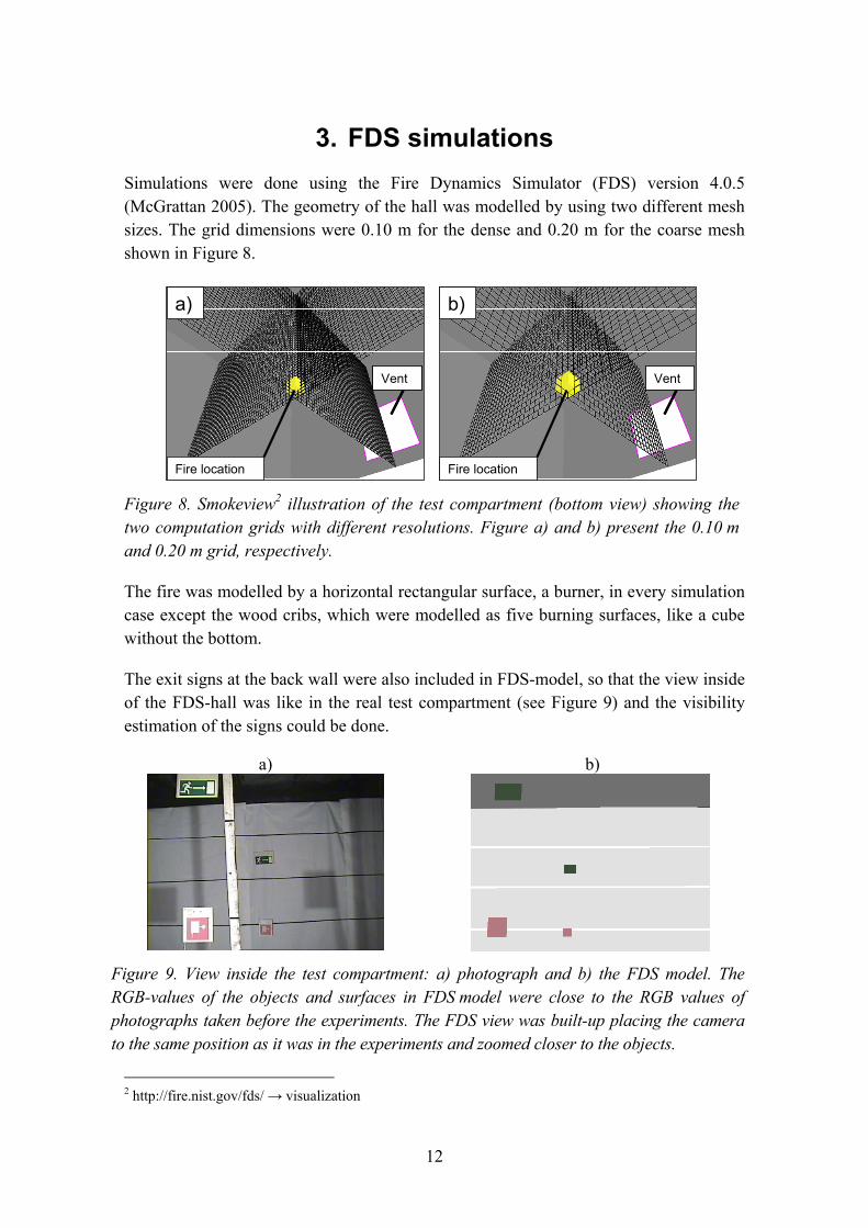
3. FDS simulations Simulations were done using the Fire Dynamics Simulator (FDS) version 4.0.5 (McGrattan 2005). The geometry of the hall was modelled by using two different mesh sizes. The grid dimensions were 0.10 m for the dense and 0.20 m for the coarse mesh shown in Figure 8.
a) b)
Fire locationFire location
VentVent VentVent
Figure 8. Smokeview2 illustration of the test compartment (bottom view) showing the two computation grids with different resolutions. Figure a) and b) present the 0.10 m and 0.20 m grid, respectively.
The fire was modelled by a horizontal rectangular surface, a burner, in every simulation case except the wood cribs, which were modelled as five burning surfaces, like a cube without the bottom.
The exit signs at the back wall were also included in FDS-model, so that the view inside of the FDS-hall was like in the real test compartment (see Figure 9) and the visibility estimation of the signs could be done.
a)
b)
Figure 9. View inside the test compartment: a) photograph and b) the FDS model. The RGB-values of the objects and surfaces in FDS model were close to the RGB values of photographs taken before the experiments. The FDS view was built-up placing the camera to the same position as it was in the experiments and zoomed closer to the objects.
2 http://fire.nist.gov/fds/ → visualization
13
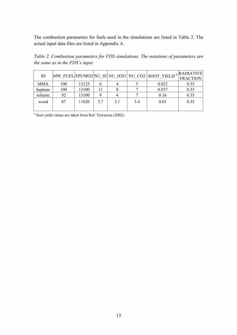
The combustion parameters for fuels used in the simulations are listed in Table 2. The actual input data files are listed in Appendix A.
Table 2. Combustion parameters for FDS simulations. The notations of parameters are the same as in the FDS�s input.
ID MW_FUEL EPUMO2 NU_02 NU_H2O NU_CO2 SOOT_YIELD a RADIATIVE FRACTION
MMA 100 13125 6 4 5 0.022 0.35 heptane 100 13100 11 8 7 0.037 0.35 toluene 92 13100 9 4 7 0.16 0.35 wood 87 11020 3.7 3.1 3.4 0.01 0.35
a Soot yield values are taken from Ref. Tewarson (2002).

14
4. Data reduction In this Chapter we present the methods used to extract information on the descent of the smoke layer and reduction of visibility due to the smoke from the data.
4.1 Determination of the smoke layer height
The analysis of the smoke layer interface height from the experiments is done by using two methods: visual analysis and analysis based on the vertical temperature profile.
Two variations of the visual analysis were used, image analysis and visual observations. The former method was used to analyse the experiments with liquid fuels (heptane and toluene) and the latter method for the experiments with solid fuels (PMMA and wood). The necessity to use different analysis methods is due to the differences in the contrasts between the background and the smoke: the smoke of the solid fuels appeared considerably whiter than the smoke of the hydro carbonaceous fuels and was hence harder to separate from the white background.
The image analysis method uses the formula
( )[ ],
maxmax k
n
IpkIpz
n
ii
im ⋅⋅=⋅⋅=∑
(1)
where zim [m] is the smoke layer height, Ii is a intensity value of a one pixel in one vertical pixel column i, maxI is the average of maximum intensity values in a whole analysing path of grey scaled image, p is the percentage value, and factor k [m] is for scaling purposes. Different p values were used for heptane and toluene. The analysing path was selected so that shadows or other effects in a picture were not disturbing the measuring. Performance of Eq. (1) is demonstrated in Figure 10.
smoke layer height
analysing path
Figure 10. Detecting the smoke layer height along the analysing path from grey scaled picture inside the hall by using Eq. (1) with p=0.55. Picture is taken 2 min after ignition. Fuel is toluene.

15
For visual observations we used the black lines drawn on the back wall of compartment (seen in Figures 10 and 7) to estimate the height of smoke layer.
Determination of the smoke-layer height from the temperature profile data is based on studies by He (1997) and He et al. (1998), where the continuous vertical temperature profile T = T(z) is defined in the region [0, H], where z = H is ceiling and z = 0 is floor. The smoke layer interface height zint is calculated by finding the height where the heat I1 integral,
( ) ( )∫ −⋅+⋅==H
ul zHTzTdzzTI0
intint1 (2)
and mass integral I2,
( ) ( )∫ −⋅+⋅==H
ul
zHT
zT
dzzT
I0
intint2111 (3)
are equal to ones resulting from the two layer approximation. In Eqs. (2) and (3) Tl is the lower layer temperature (lowest measurement point), and Tu is the upper layer temperature, respectively. Solving for zint from Eqs. (2) and (3) gives:
( )( )ll
l
HTIITHIITz212
2
221
int −+−
= . (4)
From FDS we get also estimation of the smoke layer height by using the layer height -quantity. The smoke layer height of FDS is solved using the same integral method shown in Eq. (4) (McGrattan & Forney 2005). The results of a smoke layer height of FDS in this study are presented as an average value of three points described in Appendix A.
4.2 Factors characterising visibility in a smoky environment
4.2.1 Extinction coefficient
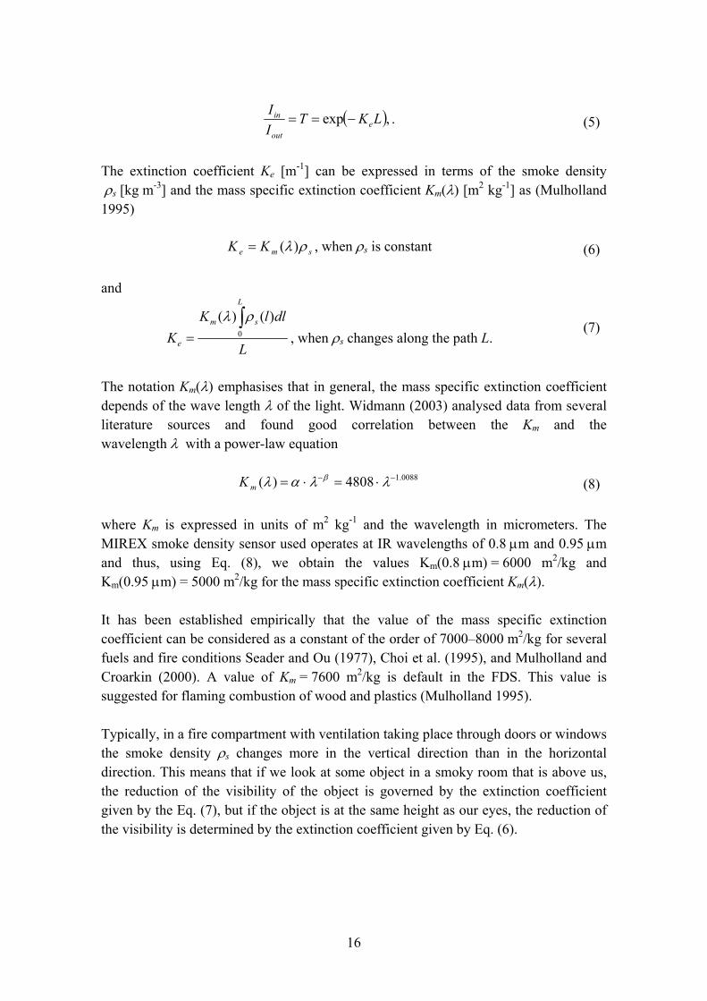
Transmission T of light through smoke is governed by the Lambert-Beer law (Hinds 1982) which states that when a light signal traverses a distance L [m], the ratio of incoming Iin and outgoing Iout signal decays exponentially as determined by the extinction coefficient Ke [m-1] characterising the transparency.
16
( ),exp LKTII
eout
in −== . (5)
The extinction coefficient Ke [m-1] can be expressed in terms of the smoke density ρs [kg m-3] and the mass specific extinction coefficient Km(λ) [m2 kg-1] as (Mulholland 1995)
sme KK ρλ)(= , when ρs is constant (6)
and
L
dllKK
L
sm
e
∫= 0
)()( ρλ, when ρs changes along the path L.
(7)
The notation Km(λ) emphasises that in general, the mass specific extinction coefficient depends of the wave length λ of the light. Widmann (2003) analysed data from several literature sources and found good correlation between the Km and the wavelength λ with a power-law equation
0088.14808)( −− ⋅=⋅= λλαλ βmK (8)
where Km is expressed in units of m2 kg-1 and the wavelength in micrometers. The MIREX smoke density sensor used operates at IR wavelengths of 0.8 µm and 0.95 µm and thus, using Eq. (8), we obtain the values Km(0.8 µm) = 6000 m2/kg and Km(0.95 µm) = 5000 m2/kg for the mass specific extinction coefficient Km(λ).
It has been established empirically that the value of the mass specific extinction coefficient can be considered as a constant of the order of 7000�8000 m2/kg for several fuels and fire conditions Seader and Ou (1977), Choi et al. (1995), and Mulholland and Croarkin (2000). A value of Km = 7600 m2/kg is default in the FDS. This value is suggested for flaming combustion of wood and plastics (Mulholland 1995).
Typically, in a fire compartment with ventilation taking place through doors or windows the smoke density ρs changes more in the vertical direction than in the horizontal direction. This means that if we look at some object in a smoky room that is above us, the reduction of the visibility of the object is governed by the extinction coefficient given by the Eq. (7), but if the object is at the same height as our eyes, the reduction of the visibility is determined by the extinction coefficient given by Eq. (6).

17
With the path length L and the mass specific extinction coefficient Km(λ) known, the soot density ρs can be obtained from experimentally determined transmission T using the Eqs. (5) and (6):
(9)
4.2.2 Visibility
Jin (1978) suggested a relation where the extinction coefficient Ke and visibility of an object V are inversely proportional. From the experiments he got a relation
3=VKe (10)
for light reflecting objects and a relation
8=VKe (11)
for light emitting objects. The FDS uses these relations for the estimation of the visibility through smoke.
4.3 Determination of the visibility and the mean extinction coefficient from the experimental data
4.3.1 Method to determine the visibility
The exit sign visibility was determined by using the grey scaled images (intensity images) extracted from the videos taken of the experiments. The fading of the exit sign into the smoke was controlled by adjusted intensity values of the grey-scale image so that when the sign was completely obscured by the smoke, the ratio rI of exit sign average intensity value sI within the whole exit sign area and the background average intensity value bI comes to 1. The average background intensity value was calculated from the area next to sign at the same height. Now, we can write the critical time tcrit to describe the exit sign fading to the smoke, Eq. (12).
(12)
The relative visibility I� (value varies between 0...1) of exit signs is calculated through Eq. (13),
( )11 ≈=⎟⎟⎠
⎞⎜⎜⎝
⎛≈= r
b
scrit It
IItt
.)(
)ln(LK
T
ms λ
ρ−
=

18
(13)
where critI (≈ 1) is the ratio of intensities at the time tcrit and Ir0 is the initial ratio of intensities (t = 0).
4.3.2 Methods to calculate the mean extinction coefficient of FDS and experiments
In Section 4.2 we discussed the reduction of visibility of light or an object in a vertical direction through the smoke. Here we describe the method used to determine the �mean� extinction coefficient from the visual data obtained in a test compartment along the path from the camera to the upper exit sign. The word �mean� is used to specify that the measured value represents a mean (or average) value over the visual path. Basically, we have available two experimental parameters: the smoke layer height zim (Eq. (1)) and the time tcrit defined in Eq. (12). The critical time tcrit gives us the visibility V in meters, which is the same as the path length, if whole path is along smoke layer. Otherwise we need information on the smoke layer height zim to calculate the length of smoky path. The path from camera to the exit sign and the analysis methods are illustrated in Figure 11.
camera
single detection point
exit sign
camera
exit sign
α
α
htot
hsmokeLtot
Lsmoke
Figure 11. The smoky path from camera to exit sing. Upper picture shows analysis used in FDS simulations and lower picture shows analysis used in the experiments.
From Figure 11 we get the relation
(14)
critr
critr
IIIII
−−
=0
'
smokee
smoke
e
smokesmoke
smoke
tot
tot
LCK
hKC
hV
hL
hL
=⇒===

19
where Ltot [m] is a distance between camera and exit sign, Lsmoke [m] is the smoky path length, same as the visibility V [m], C value is 3 (see Eq. (10)), and Ke is the extinction coefficient.
Equation (14) is used to analyse the experimental information and it is valid when the time tcrit is achieved. We also notice from Eq. (14) that if the hsmoke is equal to htot, the Ke becomes constant and does not give any further information as a function of time.
A different analysis method is used for the results from the FDS simulations as in that case have information on the local soot densities ρs(l) [kg/m3] along the smoky path L [m] from camera to the exit signs at the back wall. In this case we can calculate the extinction coefficient Ke [m-1] directly using Eq. (7) as
L
dll
L
dllKK
L
s
L
sm
e
∫∫ ⋅== 0
2
0
)(kgm 7600)()( ρρλ
. (15)
20
5. Results
5.1 Heat release rates
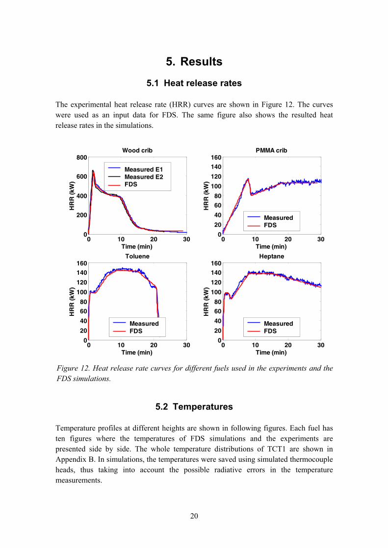
The experimental heat release rate (HRR) curves are shown in Figure 12. The curves were used as an input data for FDS. The same figure also shows the resulted heat release rates in the simulations.
0 10 20 300
200
400
600
800
Time (min)
HR
R (k
W)
Wood crib
Measured E1Measured E2FDS
0 10 20 300
20
40
60
80
100
120
140
160
Time (min)
HR
R (k
W)
PMMA crib
MeasuredFDS
0 10 20 300
20
40
60
80
100
120
140
160
Time (min)
HR
R (k
W)
Toluene
MeasuredFDS
0 10 20 300
20
40
60
80
100
120
140
160
Time (min)
HR
R (k
W)
Heptane
MeasuredFDS
Figure 12. Heat release rate curves for different fuels used in the experiments and the FDS simulations.
5.2 Temperatures
Temperature profiles at different heights are shown in following figures. Each fuel has ten figures where the temperatures of FDS simulations and the experiments are presented side by side. The whole temperature distributions of TCT1 are shown in Appendix B. In simulations, the temperatures were saved using simulated thermocouple heads, thus taking into account the possible radiative errors in the temperature measurements.
21
The temperatures of wood crib experiments E1, E2, and FDS simulations are shown in Figure 13. The simulated temperatures between heights 3.0�4.5 m seem to fit with the measured data up to 10 minutes when the cooling period starts. Just after 10 minutes the measured temperatures rise, while the same behaviour is not seen in the simulations. This may be related to the use of single value for the effective heat of combustion. In practice, the heat of combustion is much higher towards the end of the fire where the moisture of the wood has already been evaporated and the main burning solid is char. Simulated temperatures at the heights between 2.5�1.5 m differ most with the measured ones. This is probably due to the numerical diffusion associated with the prediction of smoke layer interface. The smoke layer height is not the same in experiments and simulations.
Figure 14 shows the measured and simulated temperatures during PMMA crib fire. Results are qualitatively better although the absolute temperature is not as high compared to wood crib experiments. Some differences can be seen again with the heights 2.0 m and 1.5 m where the smoke layer interface is located.
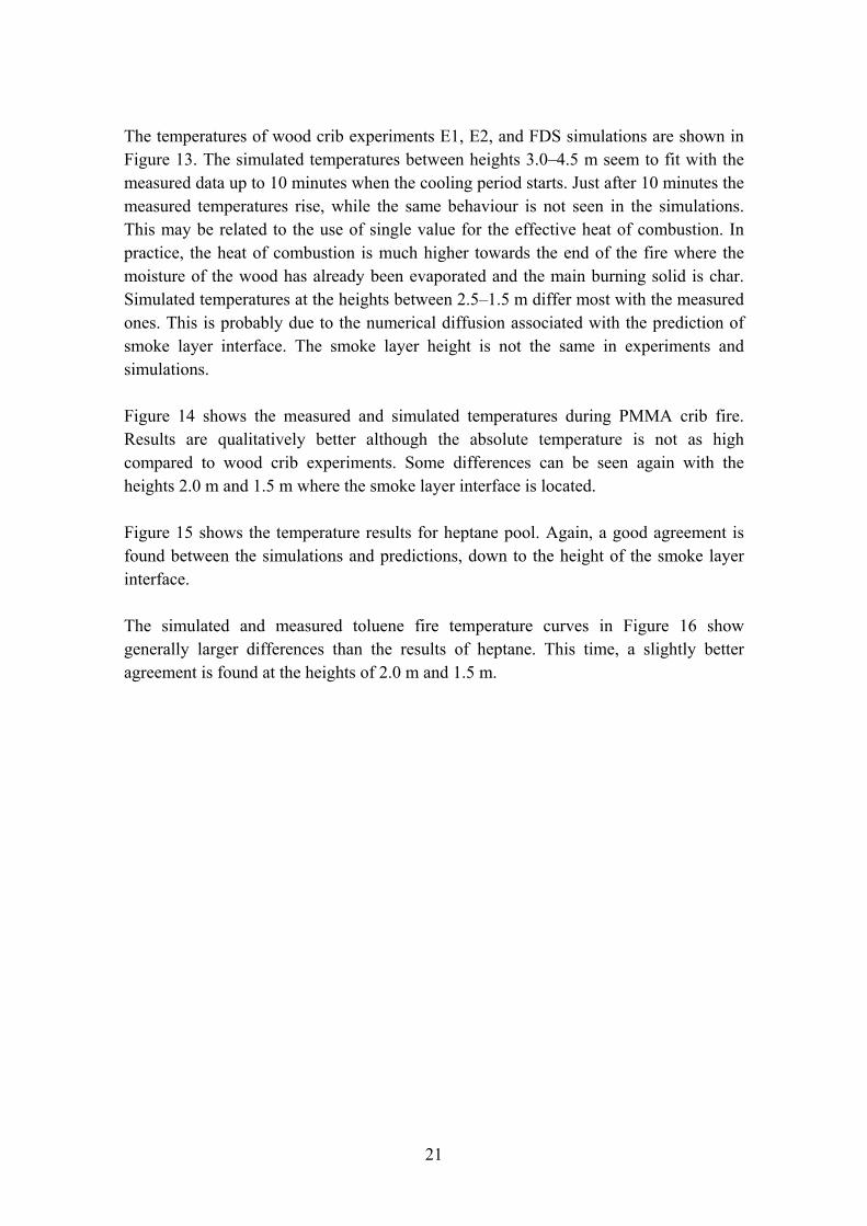
Figure 15 shows the temperature results for heptane pool. Again, a good agreement is found between the simulations and predictions, down to the height of the smoke layer interface.
The simulated and measured toluene fire temperature curves in Figure 16 show generally larger differences than the results of heptane. This time, a slightly better agreement is found at the heights of 2.0 m and 1.5 m.

22
0 10 20 300
20
40
60
80
100
120
140
Time (min)
Tem
per
atu
re (
°C)
a)
0 10 20 300
20
40
60
80
100
120
Time (min)T
emp
erat
ure
(°C
)
b)
0 10 20 300
20
40
60
80
100
120
Time (min)
Tem
per
atu
re (
°C)
c)
0 10 20 300
20
40
60
80
100
120
Time (min)
Tem
per
atu
re (
°C)
d)
0 10 20 300
20
40
60
80
100
120
Time (min)
Tem
per
atu
re (
°C)
e)
0 10 20 300
20
40
60
80
100
120
Time (min)T
emp
erat
ure
(°C
)
f)
0 10 20 300
20
40
60
Time (min)
Tem
per
atu
re (
°C)
g)
0 10 20 300
10
20
30
40
Time (min)
Tem
per
atu
re (
°C)
h)
0 10 20 300
10
20
30
40
Time (min)
Tem
per
atu
re (
°C)
i)
a) Temperature at the height of 4.5 m d) Temperature at the height of 3.0 m g) Temperature at the height of 1.5 m b) Temperature at the height of 4.0 m e) Temperature at the height of 2.5 m h) Temperature at the height of 1.0 m c) Temperature at the height of 3.5 m f) Temperature at the height of 2.0 m i) Temperature at the height of 0.5 m
TMeas. E1Meas. E2FDS 20 cm gridFDS 10 cm grid
Figure 13. Temperature profiles at different heights in the FDS simulations and the experiments. Fuel is wood. The solid and dotted lines present the temperature values obtained from TCT1 and TCT2, respectively.

23
0 10 20 300
20
40
60
Time (min)
Tem
per
atu
re (
°C)
a)
0 10 20 300
20
40
60
Time (min)T
emp
erat
ure
(°C
)
b)
0 10 20 300
20
40
60
Time (min)
Tem
per
atu
re (
°C)
c)
0 10 20 300
20
40
60
Time (min)
Tem
per
atu
re (
°C)
d)
0 10 20 300
20
40
60
Time (min)
Tem
per
atu
re (
°C)
e)
0 10 20 300
20
40
60
Time (min)T
emp
erat
ure
(°C
)
f)
0 10 20 300
10
20
30
40
Time (min)
Tem
per
atu
re (
°C)
g)
0 10 20 300
10
20
30
Time (min)
Tem
per
atu
re (
°C)
h)
0 10 20 300
10
20
30
Time (min)
Tem
per
atu
re (
°C)
i)
a) Temperature at the height of 4.5 m d) Temperature at the height of 3.0 m g) Temperature at the height of 1.5 m b) Temperature at the height of 4.0 m e) Temperature at the height of 2.5 m h) Temperature at the height of 1.0 m c) Temperature at the height of 3.5 m f) Temperature at the height of 2.0 m i) Temperature at the height of 0.5 m
M e a su r e dF D S 2 0 c m g r idF D S 1 0 c m g r id
Figure 14. Temperature profiles at different heights in the FDS simulations and the experiments. Fuel is PMMA. The solid and dotted lines present the temperature values obtained from TCT1 and TCT2, respectively.
24
0 10 20 300
20
40
60
80
Time (min)
Tem
per
atu
re (
°C)
a)
0 10 20 300
20
40
60
80
Time (min)T
emp
erat
ure
(°C
)
b)
0 10 20 300
20
40
60
80
Time (min)
Tem
per
atu
re (
°C)
c)
0 10 20 300
20
40
60
80
Time (min)
Tem
per
atu
re (
°C)
d)
0 10 20 300
20
40
60
80
Time (min)
Tem
per
atu
re (
°C)
e)
0 10 20 300
20
40
60
Time (min)T
emp
erat
ure
(°C
)
f)
0 10 20 300
10
20
30
40
Time (min)
Tem
per
atu
re (
°C)
g)
0 10 20 300
10
20
30
Time (min)
Tem
per
atu
re (
°C)
h)
0 10 20 300
10
20
30
Time (min)
Tem
per
atu
re (
°C)
i)
a) Temperature at the height of 4.5 m d) Temperature at the height of 3.0 m g) Temperature at the height of 1.5 m b) Temperature at the height of 4.0 m e) Temperature at the height of 2.5 m h) Temperature at the height of 1.0 m c) Temperature at the height of 3.5 m f) Temperature at the height of 2.0 m i) Temperature at the height of 0.5 m
M e a su r e dF D S 2 0 c m g r idF D S 1 0 c m g r id
Figure 15. Temperature profiles at different heights in the FDS simulations and the experiments. Fuel is heptane. The solid and dotted lines present the temperature values obtained from TCT1 and TCT2, respectively.

25
0 10 20 300
20
40
60
80
Time (min)
Tem
per
atu
re (
°C)
a)
0 10 20 300
20
40
60
80
Time (min)T
emp
erat
ure
(°C
)
b)
0 10 20 300
20
40
60
80
Time (min)
Tem
per
atu
re (
°C)
c)
0 10 20 300
20
40
60
80
Time (min)
Tem
per
atu
re (
°C)
d)
0 10 20 300
20
40
60
80
Time (min)
Tem
per
atu
re (
°C)
e)
0 10 20 300
20
40
60
Time (min)T
emp
erat
ure
(°C
)
f)
0 10 20 300
10
20
30
40
Time (min)
Tem
per
atu
re (
°C)
g)
0 10 20 300
10
20
30
Time (min)
Tem
per
atu
re (
°C)
h)
0 10 20 300
10
20
30
Time (min)
Tem
per
atu
re (
°C)
i)
a) Temperature at the height of 4.5 m d) Temperature at the height of 3.0 m g) Temperature at the height of 1.5 m b) Temperature at the height of 4.0 m e) Temperature at the height of 2.5 m h) Temperature at the height of 1.0 m c) Temperature at the height of 3.5 m f) Temperature at the height of 2.0 m i) Temperature at the height of 0.5 m
M e a su r e dF D S 2 0 c m g r idF D S 1 0 c m g r id
Figure 16. Temperature profiles at different heights in the FDS simulations and the experiments. Fuel is toluene. The solid and dotted lines present the temperature values obtained from TCT1 and TCT2, respectively.

26
5.3 Gas concentrations
The results of simulated and measured oxygen concentrations inside the hall are presented in Figure 17. She simulated results with 20 cm grid cells are in good agreement with results obtained with gas sampling. The results with 10 cm grid show lower oxygen values than the measured ones.
0 5 10 15 20 25 3017.5
18
18.5
19
19.5
20
20.5
21
Time (min)
O2 (
%)
Wood crib
Measured E2
Measured E1
FDS 10 cm grid
FDS 20 cm grid
0 5 10 15 20 25 30
19.5
20
20.5
21
Time (min)
O2 (
%)
PMMA crib
Measured
FDS 20 cm grid
FDS 10 cm grid
0 5 10 15 20 25 3019
19.5
20
20.5
21
Time (min)
O2 (
%)
Toluene
Measured
FDS 20 cm grid
FDS 10 cm grid
0 5 10 15 20 25 3019
19.5
20
20.5
21
Time (min)
O2 (
%)
Heptane
Measured
FDS 20 cm grid
FDS 10 cm grid
Figure 17. Oxygen concentrations in the experiments and FDS simulations.
The results of simulated and measured carbon dioxide concentrations inside the hall are presented in Figure 18. The results generally show a good agreement between the measurements and simulations with 20 cm grid. Results with toluene fuel show the simulated values being higher than the measured values. The behaviour is different with the other fuels. Comparing the two simulated values one can see the 10 cm grid values are about 0.20�0.40% higher than the values obtained from 20 cm grid.

27
0 5 10 15 20 25 300
0.5
1
1.5
2
2.5
Measured E1
Measured E2
FDS 20 cm grid
FDS 10 cm grid
Time (min)
CO
2 (%
)
Wood crib
0 5 10 15 20 25 30
0
0.2
0.4
0.6
0.8
1
Time (min)
CO
2 (%
)
PMMA crib
FDS 10 cm grid Measured
FDS 20 cm grid
0 5 10 15 20 25 300
0.2
0.4
0.6
0.8
1
1.2
Time (min)
CO
2 (%
)
Toluene
FDS 10 cm grid
Measured
FDS 20 cm grid
0 5 10 15 20 25 300
0.2
0.4
0.6
0.8
1
Time (min)
CO
2 (%
)
Heptane
FDS 10 cm grid
Measured
FDS 20 cm grid
Figure 18. Carbon dioxide concentrations in the experiments and FDS simulations.
The results of carbon monoxide concentrations are presented in Figure 19. The collapsing of wood crib in E1 occurred at the time of 14 min 20 s and in E2 at the time of 13 min 20 s. After these events the carbon monoxide yields of wood crib experiments begin to rise. Significant differences can be found between the simulated and measured values. Results with 10 cm grid are again higher than those of 20 cm grid. Carbon monoxide is a result of incomplete combustion and often difficult to model. FDS uses a correlation for carbon monoxide production, and it is linked to the soot yield input value. Here, the simulated CO-values for hydro carbonaceous fuels (toluene and heptane) are better predicted by FDS than the values of wood and PMMA. The reason might be that both wood and PMMA contain oxygen in their molecular structure and the combustion is more complete, thus yielding less carbon monoxide.

28
0 5 10 15 20 25 300
50
100
150
200
250
300
350
400Measured E1
Measured E2
FDS 20 cm grid
FDS 10 cm grid
Time (min)
CO
(p
pm
)
Wood crib
0 5 10 15 20 25 300
10
20
30
40
50
60
Measured
FDS 20 cm grid
FDS 10 cm grid
Time (min)
CO
(p
pm
)
PMMA crib
0 5 10 15 20 25 300
50
100
150
200
250
300
350
400
Time (min)
CO
(p
pm
)
Toluene
FDS 10 cm grid
Measured
FDS 20 cm grid
0 5 10 15 20 25 300
10
20
30
40
50
60
70
80
Time (min)
CO
(p
pm
)
Heptane
FDS 10 cm grid
Measured
FDS 20 cm grid
Figure 19. Carbon monoxide concentrations in the experiments and FDS simulations. CO-yield values [kg/kg] used by FDS: wood = 0.004, PMMA = 0.009, toluene = 0.060 and heptane = 0.015. The CO-yield values are taken from jobname.out file.
5.4 Smoke layer height
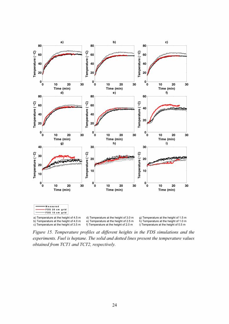
Smoke layer height in the experiments was measured by using three methods: visual observation, image analysis, and temperature profile analysis. These three methods were compared to simulated smoke layer values of FDS. The results are shown in Figure 20. From the results we can see that, in general, the smoke layer descending behaviour is very similar among the different fuels. The simulations with 20 cm grid show approximately 0.5 m lower layer heights than the values obtained from measurements. With 10 cm grid, the results are in good agreement with the measured ones. Also the two experimental curves, derived from different methods, falls to each other. From Figure 21 one can see the smoke layer does not descend lower than 2 meters during the experiments.
29
0 2 4 6 8 100
1
2
3
4
5
Experimental
FDS 20 cm grid
Visual observation
FDS 10 cm grid
Time (min)
Sm
oke
laye
r h
eig
ht
(m)
Wood crib E1
0 2 4 6 8 100
1
2
3
4
5
Time (min)
Sm
oke
laye
r h
eig
ht
(m)
Wood crib E2
Visual observation
Experimental
FDS 20 cm grid
FDS 10 cm grid
0 2 4 6 8 100
1
2
3
4
5
Time (min)
Sm
oke
laye
r h
eig
ht
(m)
PMMA crib
Experimental
Visual observation
FDS 10 cm grid
FDS 20 cm grid
0 2 4 6 8 100
1
2
3
4
5
Experimental
FDS 20 cm grid
Image analysis
FDS 10 cm grid
Time (min)
Sm
oke
laye
r h
eig
ht
(m)
Toluene
0 2 4 6 8 100
1
2
3
4
5
Time (min)
Sm
oke
laye
r h
eig
ht
(m)
Heptane
Image analysis
Experimental
FDS 20 cm grid
FDS 10 cm grid
Figure 20. Smoke layer height obtained in experiments and FDS simulations. Notation �Experimental� stands for method described in Eq. (4). The image analysis could not be used after 3 min for toluene and after 6 min for heptane and the following values are based on visual observation.

30
a) Wood crib, 10 min
b) PMMA crib, 22 min
c) Heptane pool, 10 min
d) Toluene pool, 6 min
Figure 21. Camera 2 view inside the test compartment. The red exit signs are at the height of 2 m at the level of the line shown in uppermost picture.
2 m line
31
5.5 Soot density
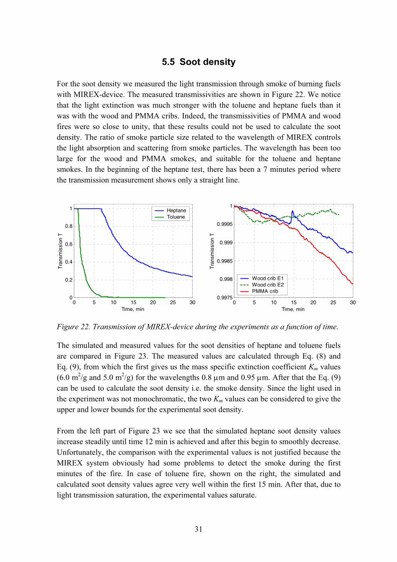
For the soot density we measured the light transmission through smoke of burning fuels with MIREX-device. The measured transmissivities are shown in Figure 22. We notice that the light extinction was much stronger with the toluene and heptane fuels than it was with the wood and PMMA cribs. Indeed, the transmissivities of PMMA and wood fires were so close to unity, that these results could not be used to calculate the soot density. The ratio of smoke particle size related to the wavelength of MIREX controls the light absorption and scattering from smoke particles. The wavelength has been too large for the wood and PMMA smokes, and suitable for the toluene and heptane smokes. In the beginning of the heptane test, there has been a 7 minutes period where the transmission measurement shows only a straight line.
0 5 10 15 20 25 300
0.2
0.4
0.6
0.8
1
Time, min
Tra
nsm
issi
on T
HeptaneToluene
0 5 10 15 20 25 300.9975
0.998
0.9985
0.999
0.9995
1
Time, min
Tra
nsm
issi
on T
Wood crib E1Wood crib E2PMMA crib
Figure 22. Transmission of MIREX-device during the experiments as a function of time.
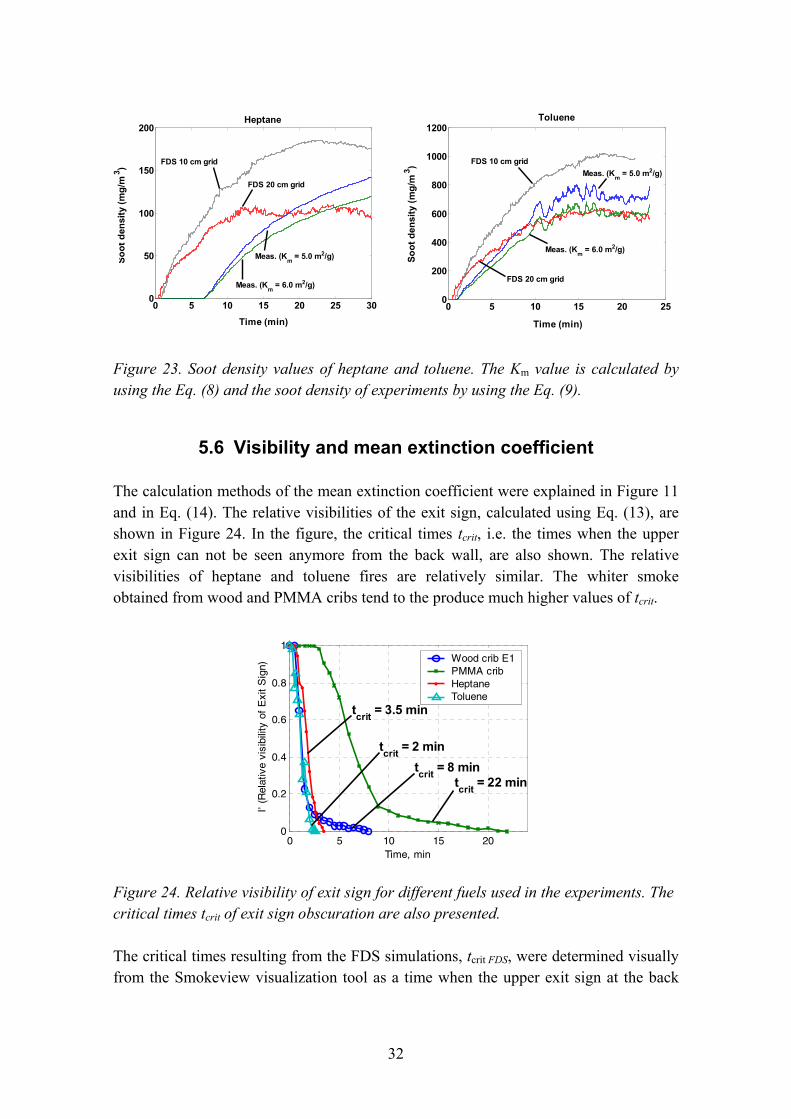
The simulated and measured values for the soot densities of heptane and toluene fuels are compared in Figure 23. The measured values are calculated through Eq. (8) and Eq. (9), from which the first gives us the mass specific extinction coefficient Km values (6.0 m2/g and 5.0 m2/g) for the wavelengths 0.8 µm and 0.95 µm. After that the Eq. (9) can be used to calculate the soot density i.e. the smoke density. Since the light used in the experiment was not monochromatic, the two Km values can be considered to give the upper and lower bounds for the experimental soot density.
From the left part of Figure 23 we see that the simulated heptane soot density values increase steadily until time 12 min is achieved and after this begin to smoothly decrease. Unfortunately, the comparison with the experimental values is not justified because the MIREX system obviously had some problems to detect the smoke during the first minutes of the fire. In case of toluene fire, shown on the right, the simulated and calculated soot density values agree very well within the first 15 min. After that, due to light transmission saturation, the experimental values saturate.
32
0 5 10 15 20 25 300
50
100
150
200So
ot d
ensi
ty (m
g/m
3 )
Time (min)
Heptane
FDS 10 cm grid
Meas. (Km = 5.0 m2/g)
Meas. (Km = 6.0 m2/g)
FDS 20 cm grid
0 5 10 15 20 25
0
200
400
600
800
1000
1200
Soot
den
sity
(mg/
m3 )
Time (min)
Toluene
Meas. (Km = 5.0 m2/g)
Meas. (Km = 6.0 m2/g)
FDS 20 cm grid
FDS 10 cm grid
Figure 23. Soot density values of heptane and toluene. The Km value is calculated by using the Eq. (8) and the soot density of experiments by using the Eq. (9).
5.6 Visibility and mean extinction coefficient
The calculation methods of the mean extinction coefficient were explained in Figure 11 and in Eq. (14). The relative visibilities of the exit sign, calculated using Eq. (13), are shown in Figure 24. In the figure, the critical times tcrit, i.e. the times when the upper exit sign can not be seen anymore from the back wall, are also shown. The relative visibilities of heptane and toluene fires are relatively similar. The whiter smoke obtained from wood and PMMA cribs tend to the produce much higher values of tcrit.
0 5 10 15 200
0.2
0.4
0.6
0.8
1
I' (R
elat
ive
visi
bilit
y of
Exi
t S
ign)
Time, min
Wood crib E1PMMA crib Heptane Toluene
tcrit = 22 min tcrit = 8 min
tcrit = 3.5 min
tcrit = 2 min
Figure 24. Relative visibility of exit sign for different fuels used in the experiments. The critical times tcrit of exit sign obscuration are also presented.
The critical times resulting from the FDS simulations, tcrit FDS, were determined visually from the Smokeview visualization tool as a time when the upper exit sign at the back

33
wall was faded. The experimental and simulation-based critical times are compared in Figure 25. For the heptane and toluene fuels, the simulated and measured times are in very close agreement, but for the wood and PMMA fuels, the simulated obscurations take place too early. For the practical applications, Smokeview provides two means to adjust the visual representation of the 3D smoke: Smoke Thickness and Gray Level. By changing the Gray Level parameter from the default value of 0 to a value 70 for the PMMA and to a value 140 for the wood, the simulation based critical times could be adjusted close to the measured values, as shown by the grey dots in Figure 25.
0
5
10
15
20
25
0 5 10 15 20 25
FDS tcrit FDS (min)
Mea
sure
d t cr
it (m
in)
PMMAHEPTANEWOODTOLUENEWOODPMMA
Figure 25. Comparison of the simulated (tcrit FDS) and measured (tcrit) obscuration times of upper exit sign at the back wall. The black dots were obtained by using the default Smoke3D parameters in Smokeview and the grey dots with adjusted parameters.
From the critical times and the experimental smoke layer heights (Chapter 5.4) we can estimate the mean extinction coefficient Ke along the optical path from the camera to the upper exit sign by using Eq. (14) for the experimental data and Eq. (15) for FDS results. In Figure 26, two sets of Ke values have been plotted from simulations using the 20 cm grid size. The first set, �the experimental-based approach� (open symbols), was derived by integrating the FDS soot density output at the experimental tcrit. The corresponding soot density data are shown as solid lines in Figure 27. The second data set called �Smokeview-based approach� (black symbols in Figure 26) is determined by integrating the FDS soot density data at the time of tcrit FDS. The corresponding soot density data are shown as dashed lines in Figure 27. Both data sets are plotted against the measured extinction coefficients. In the analysis of wood and PMMA results, we assumed that the smoke layer covered the whole path from the camera to the upper exit sign at the back wall (see Figure 11). As a result, these fuels have the same value of extinction coefficient. According to the results shown in Figure 26, the experimental and �Smokeview-based� simulated mean extinction coefficients are in satisfactory

34
agreement for all the fuel except toluene. In case of �experimental-based� approach, only heptane and toluene results are satisfactory.
0
0.2
0.4
0.6
0.8
1
1.2
1.4
0.0 0.2 0.4 0.6 0.8 1.0 1.2 1.4
FDS Ke (m-1)
Mea
sure
d K
e (m
-1)
PMMAPMMAHEPTANEHEPTANEWOODWOODTOLUENETOLUENE
Figure 26. Measured and simulated values of extinction coefficient Ke. Open symbols present the �experimental-based� approach and the black symbols the �Smokeview-based� approach, as explained in the text.
0 2 4 6 8 100
50
100
150
200
Path length from camera1 to exit sign, m
Soo
t de
nsity
, m
g/m
3
PMMA wood tolueneheptane
Figure 27. Soot density along the smoky path from camera to the upper exit sign in FDS simulations. The solid lines correspond to the time tcrit and the dashed lines to the time tcrit FDS.
35
6. Summary In this study we have validated experimentally the capability of Fire Dynamics Simulator (FDS version 4.0.5) to predict the smoke properties inside a test compartment for predefined burning rates of wood, PMMA, heptane, and toluene fuels. The studied smoke properties were soot and gas concentrations and vertical gas temperature profiles. The validation was performed by comparing the simulation results to the measured ones.
The simulated temperature profiles were generally in very good agreement with the experimental results. The highest deviations between the simulated and measured values were found at the height of the smoke layer interface. From the smoke layer height measurements we noticed that the simulated values with 20 cm grid size were about 0.5 m lower than the measured values. In this case, the error is about 10% of the total room height.
The simulated and measured concentrations of carbon dioxide and oxygen were also in good agreement. The results from carbon monoxide showed that the FDS�s correlation for CO production performed quite well in case of the hydro carbonaceous fuels (heptane and toluene) and rather poorly in case of the solid fuels (wood and PMMA).
The smoke production and the light extinction inside the compartment were monitored by cameras and by an optical instrument MIREX. The wavelength range 800�950 nm was found appropriate for the light transmission measurement for the hydro carbonaceous fuels. A good agreement was found between the measured and simulated soot density values in case of toluene fuel. For other fuels, the uncertainties of the optical measurements were too high to draw any conclusions.
In case of the hydrocarbonaceous fuels (heptane and toluene), the critical times of exit sign obscuration, determined from the Smokeview visualizations, were in good agreement with the values determined from the video images. For such fuels, the use of default values of Smokeview and FDS leads to good predictions of the view inside a fire compartment. For solid fuels (wood and PMMA) producing smoke that is more gray in colour, the necessary adjustments of the Gray Level visualization parameter were given in order to match the visualizations and video images of the exit sign obscuration. The analysis of the visually determined mean extinction coefficients showed that the visual representation of the FDS simulations is consistent with the physical output.

36
Acknowledgements Authors like to thank Mr. Konsta Taimisalo and Mr. Risto Latva for their skilled work of building up the experimental set up.

37
References Choi, M. Y., Mulholland, G. W., Hamins, A. and Kashiwagi, T. 1995. Comparisons of the Soot Volume Fraction Using Gravimetric and Light Extinction Techniques. Combustion and Flame, Vol. 102, pp. 161�169.
He, Y. 1997. On Experimental Data Reduction for Zone Model Validation. Journal of Fire Sciences, Vol. 15, pp. 144�161.
He, Y., Fernando, A. & Luo, M. 1998. Determination of interface height from measured parameter profile in enclosure fire experiment. Fire Safety Journal, Vol. 31, pp. 19�38.
Hinds, W. 1982. Aerosol technology: properties, behavior, and measurement of airborne particles. New York: John Wiley. 424 p.
Jin, T. 1978. Visibility Trough Fire Smoke. Journal of Fire & Flammability, Vol. 9, pp. 135�155.
McGrattan, K. 2005. Fire Dynamics Simulator (Version 4) � Technical Reference Guide. Special Publication 1018. Gaithersburg, MD: National Institute of Standards and Technology. 96 p.
McGrattan, K. & Forney, G. 2005. Fire Dynamics Simulator (Version 4) � User�s Guide. Special Publication 1019. Gaithersburg, MD: National Institute of Standards and Technology. 90 p.
Mulholland, G. 1995. Smoke production and properties. In: DiNenno, P. et al. (eds.). SFPE Handbook of Fire Protection Engineering. 2nd Ed. Quincy, MA: National Fire Protection Association. Pp. 2-217�2-227.
Mulholland, G. & Croarkin, C. 2000. Specific Extinction Coefficient of Flame Generated Smoke. Fire and Materials, Vol. 24, pp. 227�230.
Seader, J. & Ou, S. 1977. Correlation of the Smoking Tendency of Materials. Fire Research, Vol. 1, pp. 3�9.
Tewarson, A. 2002. Generation of Heat and Chemical Compounds in Fires. The SFPE Handbook of Fire Protection Engineering. 3rd ed. Section 3, Chapter 4. Quincy, MA: The National Fire Protection Association Press. Pp. 3-82�3-161.
Widmann, J. 2003. Evaluation of the Planck mean absorption coefficients for radiation transport through smoke. Combustion Science and Technology, Vol. 175, pp. 2299�2308.
A/1
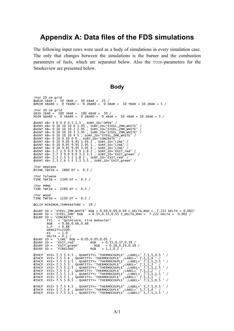
Appendix A: Data files of the FDS simulations The following input rows were used as a body of simulations in every simulation case. The only that changes between the simulations is the burner and the combustion parameters of fuels, which are separated below. Also the TOUR-parameters for the Smokeview are presented below.
Body
/For 20 cm grid &GRID IBAR = 50 JBAR = 50 KBAR = 25 / &PDIM XBAR0 = 0 YBAR0 = 0 ZBAR0 = 0 XBAR = 10 YBAR = 10 ZBAR = 5 / /For 10 cm grid GRID IBAR = 100 JBAR = 100 KBAR = 50 / PDIM XBAR0 = 0 YBAR0 = 0 ZBAR0 = 0 XBAR = 10 YBAR = 10 ZBAR = 5 / &VENT XB= 4 6 0 0 0.5 2.5 , SURF_ID='OPEN' / &VENT XB= 0 10 10 10 0 1.95 , SURF_ID='STEEL_2MM_WHITE' / &VENT XB= 0 10 10 10 2 2.95 , SURF_ID='STEEL_2MM_WHITE' / &VENT XB= 0 10 10 10 3 3.95 , SURF_ID='STEEL_2MM_WHITE' / &VENT XB= 0 10 10 10 4 5 , SURF_ID='STEEL_2MM_WHITE' / &VENT XB= 0 10 0 10 0 0 , SURF_ID='CONCRETE' / &VENT XB= 0 10 9.95 9.95 1.95 2 , SURF_ID='LINE' / &VENT XB= 0 10 9.95 9.95 2.95 3 , SURF_ID='LINE' / &VENT XB= 0 10 9.95 9.95 3.95 4 , SURF_ID='LINE' / &VENT XB= 2.7 2.9 9.9 9.9 1.8 2 , SURF_ID='EXIT_red' / &VENT XB= 2.7 3 9.9 9.9 3.3 3.5 , SURF_ID='EXIT_green' / &VENT XB= 2.3 2.5 5 5 1.8 2 , SURF_ID='EXIT_red' / &VENT XB= 2.3 2.6 5 5 3.3 3.5 , SURF_ID='EXIT_green' / /For Heptane &TIME TWFIN = 1860 DT = 0.5 / /For Toluene TIME TWFIN = 1349 DT = 0.5 / /For PMMA TIME TWFIN = 2160 DT = 0.5 / /For Wood TIME TWFIN = 1250 DT = 0.5 / &CLIP MINIMUM_TEMPERATURE = 19 / &SURF ID = 'STEEL_2MM_WHITE' RGB = 0.69,0.69,0.69 C_DELTA_RHO = 7.222 DELTA = 0.002/ &SURF ID = 'STEEL_2MM' RGB = 0.55,0.55,0.55 C_DELTA_RHO = 7.222 DELTA = 0.002 / &SURF ID = 'CONCRETE' FYI = 'Quintiere, Fire Behavior' RGB = 0.66,0.66,0.66 C_P = 0.88 DENSITY=2100. KS = 1.0 DELTA = 0.1 / &SURF ID = 'LINE' RGB = 0.05,0.05,0.05 / &SURF ID = 'EXIT_red' RGB = 0.55,0.37,0.39 / &SURF ID = 'EXIT_green' RGB = 0.18,0.24,0.18 / &SURF ID = 'FIRELOAD' RGB = 1,1,0.2 / &THCP XYZ= 7.5 5 4.5 , QUANTITY= 'THERMOCOUPLE' ,LABEL=' 7.5_5_4.5 ' / &THCP XYZ= 7.5 5 4 , QUANTITY= 'THERMOCOUPLE' ,LABEL=' 7.5_5_4 ' / &THCP XYZ= 7.5 5 3.5 , QUANTITY= 'THERMOCOUPLE' ,LABEL=' 7.5_5_3.5 ' / &THCP XYZ= 7.5 5 3 , QUANTITY= 'THERMOCOUPLE' ,LABEL=' 7.5_5_3 ' / &THCP XYZ= 7.5 5 2.5 , QUANTITY= 'THERMOCOUPLE' ,LABEL=' 7.5_5_2.5 ' / &THCP XYZ= 7.5 5 2 , QUANTITY= 'THERMOCOUPLE' ,LABEL=' 7.5_5_2 ' / &THCP XYZ= 7.5 5 1.5 , QUANTITY= 'THERMOCOUPLE' ,LABEL=' 7.5_5_1.5 ' / &THCP XYZ= 7.5 5 1 , QUANTITY= 'THERMOCOUPLE' ,LABEL=' 7.5_5_1 ' / &THCP XYZ= 7.5 5 0.5 , QUANTITY= 'THERMOCOUPLE' ,LABEL=' 7.5_5_0.5 ' / &THCP XYZ= 5 7.5 4.5 , QUANTITY= 'THERMOCOUPLE' ,LABEL=' 5_7.5_4.5 ' / &THCP XYZ= 5 7.5 4 , QUANTITY= 'THERMOCOUPLE' ,LABEL=' 5_7.5_4 ' / &THCP XYZ= 5 7.5 3.5 , QUANTITY= 'THERMOCOUPLE' ,LABEL=' 5_7.5_3.5 ' /
A/2
&THCP XYZ= 5 7.5 3 , QUANTITY= 'THERMOCOUPLE' ,LABEL=' 5_7.5_3 ' / &THCP XYZ= 5 7.5 2.5 , QUANTITY= 'THERMOCOUPLE' ,LABEL=' 5_7.5_2.5 ' / &THCP XYZ= 5 7.5 2 , QUANTITY= 'THERMOCOUPLE' ,LABEL=' 5_7.5_2 ' / &THCP XYZ= 5 7.5 1.5 , QUANTITY= 'THERMOCOUPLE' ,LABEL=' 5_7.5_1.5 ' / &THCP XYZ= 5 7.5 1 , QUANTITY= 'THERMOCOUPLE' ,LABEL=' 5_7.5_1 ' / &THCP XYZ= 5 7.5 0.5 , QUANTITY= 'THERMOCOUPLE' ,LABEL=' 5_7.5_0.5 ' / &THCP XYZ= 7.5 7.5 3.5 , QUANTITY= 'soot density' ,LABEL=' 7.5_7.5_3.5 ' / &THCP XYZ= 3 8 3.5 , QUANTITY= 'LAYER HEIGHT' ,LABEL=' 3_8_3.5 ' / &THCP XYZ= 3 8 3.5 , QUANTITY= 'LAYER HEIGHT' ,LABEL=' 5_8_3.5 ' / &THCP XYZ= 3 8 3.5 , QUANTITY= 'LAYER HEIGHT' ,LABEL=' 7.5_8_3.5 ' / &THCP XYZ= 3 1 1.8 , QUANTITY= 'soot density' ,LABEL=' 3_1_1.8 ' / &THCP XYZ= 3 1.5 1.89 , QUANTITY= 'soot density' ,LABEL=' 3_1.5_1.89 ' / &THCP XYZ= 3 2 1.99 , QUANTITY= 'soot density' ,LABEL=' 3_2_1.99 ' / &THCP XYZ= 3 2.5 2.08 , QUANTITY= 'soot density' ,LABEL=' 3_2.5_2.08 ' / &THCP XYZ= 3 3 2.18 , QUANTITY= 'soot density' ,LABEL=' 3_3_2.18 ' / &THCP XYZ= 3 3.5 2.27 , QUANTITY= 'soot density' ,LABEL=' 3_3.5_2.27 ' / &THCP XYZ= 3 4 2.37 , QUANTITY= 'soot density' ,LABEL=' 3_4_2.37 ' / &THCP XYZ= 3 4.5 2.46 , QUANTITY= 'soot density' ,LABEL=' 3_4.5_2.46 ' / &THCP XYZ= 3 5 2.56 , QUANTITY= 'soot density' ,LABEL=' 3_5_2.56 ' / &THCP XYZ= 3 5.5 2.65 , QUANTITY= 'soot density' ,LABEL=' 3_5.5_2.65 ' / &THCP XYZ= 3 6 2.74 , QUANTITY= 'soot density' ,LABEL=' 3_6_2.74 ' / &THCP XYZ= 3 6.5 2.84 , QUANTITY= 'soot density' ,LABEL=' 3_6.5_2.84 ' / &THCP XYZ= 3 7 2.93 , QUANTITY= 'soot density' ,LABEL=' 3_7_2.93 ' / &THCP XYZ= 3 7.5 3.03 , QUANTITY= 'soot density' ,LABEL=' 3_7.5_3.03 ' / &THCP XYZ= 3 8 3.12 , QUANTITY= 'soot density' ,LABEL=' 3_8_3.12 ' / &THCP XYZ= 3 8.5 3.22 , QUANTITY= 'soot density' ,LABEL=' 3_8.5_3.22 ' / &THCP XYZ= 3 9 3.31 , QUANTITY= 'soot density' ,LABEL=' 3_9_3.31 ' / &THCP XYZ= 3 9.5 3.41 , QUANTITY= 'soot density' ,LABEL=' 3_9.5_3.41 ' / &THCP XYZ= 3 10 3.5 , QUANTITY= 'soot density' ,LABEL=' 3_10_3.5 ' / &THCP XYZ= 9 7.5 3.5 , QUANTITY= 'oxygen' ,LABEL=' 9_7.5_3.5 ' / &THCP XYZ= 9 7.5 3.5 , QUANTITY= 'carbon dioxide' ,LABEL=' 9_7.5_3.5 ' / &THCP XYZ= 9 7.5 3.5 , QUANTITY= 'carbon monoxide' ,LABEL=' 9_7.5_3.5 ' /
PMMA
&REAC ID='MMA' FYI='MMA monomer, C_5 H_8 O_2' EPUMO2=13125. MW_FUEL=100. NU_O2=6. NU_H2O=4. NU_CO2=5. SOOT_YIELD=0.022 / &MISC REACTION='MMA' SMOKE3D = .TRUE. NFRAMES = 2160 SURF_DEFAULT= 'STEEL_2MM' / &RADI NUMBER_RADIATION_ANGLES = 50 / &SURF ID='BURNER' HRRPUA = 426.8 RAMP_Q = 'TR' TMPWAL = 300 RGB = 1,0.5,0 / &RAMP ID = 'TR' T = 60 ,F = 0 / &RAMP ID = 'TR' T = 528 ,F = 1.091 / &RAMP ID = 'TR' T = 588 ,F = 0.746/ &RAMP ID = 'TR' T = 1158 ,F = 1 / &RAMP ID = 'TR' T = 1860 ,F = 1 / &RAMP ID = 'TR' T = 2160 ,F = 0 / &OBST XB = 4.75 5.25 4.75 5.25 0.1 0.4 , SURF_ID='FIRELOAD' / &VENT XB = 4.75 5.25 4.75 5.25 0.4 0.4 ,IOR = 3 SURF_ID = 'BURNER' /

A/3
Wood
&REAC ID='WOOD' FYI='Ritchie, et al., 5th IAFSS, C_3.4 H_6.2 O_2.5' SOOT_YIELD = 0.01 NU_O2 = 3.7 NU_CO2 = 3.4 NU_H2O = 3.1 MW_FUEL = 87. EPUMO2 = 11020. / &MISC REACTION='WOOD' SMOKE3D = .TRUE. NFRAMES = 1250 SURF_DEFAULT= 'STEEL_2MM' / &RADI NUMBER_RADIATION_ANGLES = 50 / &SURF ID='BURNER' HRRPUA = 540 RAMP_Q = 'TR' TMPWAL = 300 RGB = 1,0.5,0 / &RAMP ID = 'TR' T = 60 ,F = 0 / &RAMP ID = 'TR' T = 155.4 ,F = 1 / &RAMP ID = 'TR' T = 187.2 ,F = 0.75/ &RAMP ID = 'TR' T = 394.2 ,F = 0.61 / &RAMP ID = 'TR' T = 658.2 ,F = 0.56 / &RAMP ID = 'TR' T = 846 ,F = 0.22 / &RAMP ID = 'TR' T = 954.6 ,F = 0.1 / &RAMP ID = 'TR' T = 1250.4 ,F = 4.44E-02 / &OBST XB = 4.75 5.25 4.75 5.25 0.3 0.8 , SURF_ID='FIRELOAD' / &VENT XB = 4.75 5.25 4.75 5.25 0.8 0.8 ,IOR = 3 SURF_ID = 'BURNER'/ &VENT XB = 4.75 4.75 4.75 5.25 0.3 0.8 ,IOR = -1 SURF_ID = 'BURNER'/ &VENT XB = 4.75 5.25 5.25 5.25 0.3 0.8 ,IOR = 2 SURF_ID = 'BURNER'/ &VENT XB = 5.25 5.25 4.75 5.25 0.3 0.8 ,IOR = 1 SURF_ID = 'BURNER'/ &VENT XB = 4.75 5.25 4.75 4.75 0.3 0.8 ,IOR = -2 SURF_ID = 'BURNER'/
Heptane
&REAC ID='HEPTANE' FYI='Heptane, C_7 H_16' MW_FUEL=100. NU_O2=11. NU_CO2=7. NU_H2O=8. SOOT_YIELD=0.037 / &MISC REACTION='HEPTANE' SMOKE3D = .TRUE. NFRAMES = 1860 SURF_DEFAULT= 'STEEL_2MM' / &RADI NUMBER_RADIATION_ANGLES = 50 / &SURF ID='BURNER' HRRPUA = 1548.8 RAMP_Q = 'TR' TMPWAL = 300 RGB = 1,0.5,0 / &RAMP ID = 'TR' T = 60 ,F = 0 / &RAMP ID = 'TR' T = 75 ,F = 0.50/ &RAMP ID = 'TR' T = 99 ,F = 0.70/ &RAMP ID = 'TR' T = 159 ,F = 0.70/ &RAMP ID = 'TR' T = 219 ,F = 0.60/ &RAMP ID = 'TR' T = 540 ,F = 1 / &RAMP ID = 'TR' T = 960 ,F = 1 / &RAMP ID = 'TR' T = 1860 ,F = 0.79/ &RAMP ID = 'TR' T = 1860 ,F = 0 / &OBST XB = 4.85 5.15 4.85 5.15 0.2 0.5 , SURF_ID='FIRELOAD' / &VENT XB = 4.85 5.15 4.85 5.15 0.5 0.5 ,IOR = 3 SURF_ID = 'BURNER'/
A/4
Toluene
&REAC ID='TOLUENE' FYI='Toluene, C_7 H_8' MW_FUEL=92. NU_O2=9. NU_CO2=7. NU_H2O=4. RADIATIVE_FRACTION=0.43 SOOT_YIELD=0.16 / &MISC REACTION='TOLUENE' SMOKE3D = .TRUE. NFRAMES = 1349 SURF_DEFAULT= 'STEEL_2MM' / &RADI NUMBER_RADIATION_ANGLES = 50 / &SURF ID='BURNER' HRRPUA = 1618.8 RAMP_Q = 'TR' TMPWAL = 300 RGB = 1,0.5,0 &RAMP ID = 'TR' T = 60 ,F = 0 / &RAMP ID = 'TR' T = 71.4 ,F = 0.617 / &RAMP ID = 'TR' T = 99 ,F = 0.673/ &RAMP ID = 'TR' T = 202.2 ,F = 0.673 / &RAMP ID = 'TR' T = 399 ,F = 0.915/ &RAMP ID = 'TR' T = 577.8 ,F = 1 / &RAMP ID = 'TR' T = 960 ,F = 0.988/ &RAMP ID = 'TR' T = 1309.2 ,F = 0.754 / &RAMP ID = 'TR' T = 1349.4 ,F = 0 / &OBST XB = 4.85 5.15 4.85 5.15 0.2 0.5 , SURF_ID='FIRELOAD' / &VENT XB = 4.85 5.15 4.85 5.15 0.5 0.5 ,IOR = 3 SURF_ID = 'BURNER'/
TOUR-parameters for the Smokeview
These parameters make camera position and the view of the Smokeview inside the hall similar whit the experiments in this study. Parameters must locate in jobname.ini -file.
Tour 2 2 1 0.000000 0.0 3.389927 1.043823 1.811231 0 37.779999 11.157625 0.0 0.0 0.0 0.0 2.411406 0 7680.0 11.0 11.0 2.5 0 0.0 0.0 0.0 0.0 0.0 0.0 1.0 0

B/1
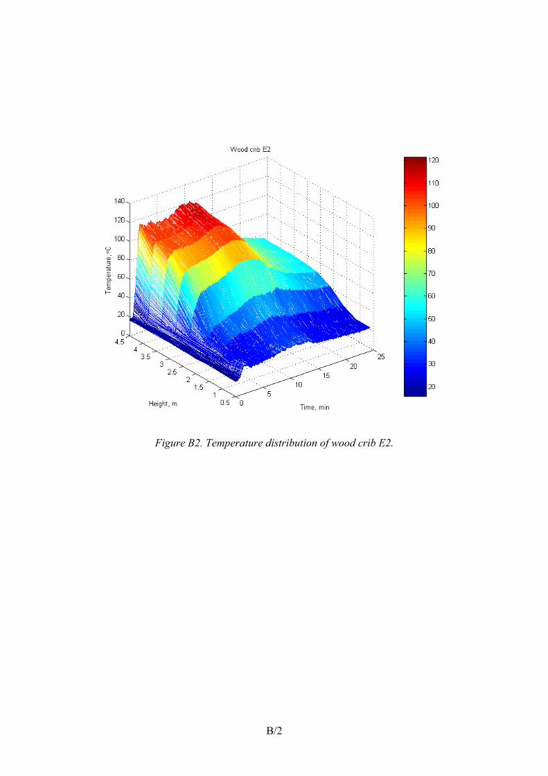
Appendix B: Temperature distributions of the experiments
Following figures (Figures B1�B5) present the temperature distributions during the experiments at the placement of first thermocouple tree (TCT1) as a function of time.
Figure B1. Temperature distribution of wood crib E1.
B/2
Figure B2. Temperature distribution of wood crib E2.

B/3
Figure B3. Temperature distribution of heptane.

B/4
Figure B4. Temperature distribution of toluene.

B/5
Figure B5. Temperature distribution of PMMA crib.

ISBN 978-951-38-6617-4 (URL: http://www.vtt.fi/publications/jsp) ISSN 1459-7683 (URL: http://www.vtt.fi/ publications/jsp)
VTT Working papers
43 Tsupari, Eemeli, Tormonen, Kauko, Monni, Suvi, Vahlman, Tuula, Kolsi, Aimo & Linna, Veli. Dityppioksidin (N2O) ja metaanin (CH4) päästökertoimia Suomen voimalaitoksille, lämpö�keskuksille ja pienpoltolle. 2006. 94 s. + liitt. 7 s.
44 Saarinen, Jani, Rilla, Nina, Loikkanen, Torsti, Oksanen, Juha & Alasaarela, Jaakko. Innovaatio�ympäristö tänään ja huomenna. 2006. 32 s.
45 Heinonen, Jaakko. Preliminary Study of Modelling Dynamic Properties of Magnetorheological Fluid Damper. 2006. 36 p.
46 Häkkinen, Kai & Salmela, Erno. Logistiikkapalveluyhtiömalleja Suomen metalliteollisuudessa. Havaintoja vuonna 2005. SERVIISI-projektin osaraportti. 2006. 17 s.
47 Kurtti, Reetta & Reiman, Teemu. Organisaatiokulttuuri logistiikkapalveluorganisaatiossa. Tutkimus viidessä palveluvarastossa. 2006. 30 s.
48 Soimakallio, Sampo, Perrels, Adriaan, Honkatukia, Juha, Moltmann, Sara & Höhne, Niklas. Analysis and Evaluation of Triptych 6. Case Finland. 2006. 70 p. + app. 8 p.
49 Saarinen, Jani, Rilla, Nina, Loikkanen, Torsti, Oksanen, Juha & Alasaarela, Jaakko. Innovation environment today and tomorrow. 2006. 32 p.
50 Törnqvist, Jouko & Talja, Asko. Suositus liikennetärinän arvioimiseksi maankäytön suunnit�telussa. 2006. 46 s. + liitt. 33 s.
51 Aikio, Sanna, Grönqvist, Stina, Hakola, Liisa, Hurme, Eero, Jussila, Salme, Kaukoniemi, Otto-Ville, Kopola, Harri, Känsäkoski, Markku, Leinonen, Marika, Lippo, Sari, Mahlberg, Riitta, Peltonen, Soili, Qvintus-Leino, Pia, Rajamäki, Tiina, Ritschkoff, Anne-Christine, Smolander, Maria, Vartiainen, Jari, Viikari, Liisa & Vilkman, Marja. Bioactive paper and fibre products. Patent and literary survey. 2006. 83 p.
52 Alanen, Raili & Hätönen, Hannu. Sähkön laadun ja jakelun luotettavuuden hallinta. State of art -selvitys. 2006. 84 s.
53 Pasonen, Markku & Hakkarainen, Toni. Kaukolämpölinjojen elinikä ja NDT. 2006. 27 s. 54 Hietaniemi, Jukka, Toratti, Tomi, Schnabl, Simon & Turk, Goran. Application of reliability analysis
and fire simulation to probabilistic assessment of fire endurance of wooden structures. 2006. 97 p. + app. 23 p.
55 Holttinen, Hannele. Tuulivoiman tuotantotilastot. Vuosiraportti 2005. 2006. 38 s. + liitt. 7 s. 56 Häkkinen, Kai, Hemilä, Jukka, Salmela, Erno & Happonen, Ari. Logistiikka Belgiassa.
Vierailukokemuksia keväältä 2006. 2006. 33 s. 57 Kulmala, Risto. Tiehallinto ja liikenteen tietopalvelut. Selvitysmiehen muistio. 2006. 29 s. + liitt. 3 s. 59 Graczykowski, Cezary & Heinonen, Jaakko. Adaptive Inflatable Structures for protecting wind
turbines against ship collisions. 2006. 86 p. + app. 39 p. 60 Känsäkoski, Markku, Kurkinen, Marika, von Weymarn, Niklas, Niemelä, Pentti, Neubauer, Peter,
Juuso, Esko, Eerikäinen, Tero, Turunen, Seppo, Aho, Sirkka & Suhonen, Pirkko. Process analytical technology (PAT) needs and applications in the bioprocess industry. Review. 2006. 99 p.
61 Välisalo, Tero, Räikkönen, Minna & Lehtinen, Erkki. Asset Management vesihuollossa. Kirjal�lisuustutkimus. 2006. 79 s. + liitt. 8 s.
62 Holt, Erika. Current trends in USA building research. 2006. 26 p. + app. 7 p. 64 Forsström, Juha. Ydinjätehuollon kustannusriskianalyysi. Esitutkimus. 2006. 51 p. 65 Talja, Asko, Törnqvist, Jouko, Kivikoski, Harri, Carpén, Leena & Nippala, Eero. Ruostumaton
teräs maa- ja vesirakentamisessa. 2006. 32 s. + liitt. 5 s. 66 Rinne, Tuomo, Hietaniemi, Jukka & Hostikka, Simo. Experimental Validation of the FDS
Simulations of Smoke and Toxic Gas Concentrations. 2007. 37 p. + app. 9 p.
Top Related