


Languages
Pages
Legal


Evaluation of Top-k Queries over Structured and
Semi-structured Data
Amelie Marian
Submitted in partial fulfillment of the
requirements for the degree
of Doctor of Philosophy
in the Graduate School of Arts and Sciences
COLUMBIA UNIVERSITY
2005

c©2005
Amelie Marian
All Rights Reserved
ABSTRACT
Evaluation of Top-k Queries over Structured and
Semi-structured Data
Amelie Marian
Traditionally, queries over structured (e.g., relational) and semi-structured (e.g., XML)
data identify the exact matches for the queries. This exact-match query model is not ap-
propriate for many database applications and scenarios where queries are inherently fuzzy
—often expressing user preferences and not hard Boolean constraints— and are best an-
swered with a ranked, or “top-k,” list of the best matching objects. The top-k query model
is widely used in web search engines and information retrieval systems over (relatively un-
structured) text data. This thesis addresses fundamental issues in defining and efficiently
processing top-k queries for a variety of scenarios, presenting different query processing
challenges. In all these scenarios, our query processing algorithms attempt to focus on the
objects that are most likely to be among the top-k matches for a given query, and discard
—as early as possible— objects that are guaranteed not to qualify for the top-k answer,
thus minimizing query processing time.
One important top-k query scenario that we study is web applications where the data
objects are only available through remote, autonomous web sources. During query pro-
cessing, these sources have to be queried repeatedly for a potentially large set of candidate
objects. Processing top-k queries efficiently in such a scenario is challenging, as web sources
exhibit diverse probing costs and access interfaces, as well as constraints on the degree of
concurrency that they support. By considering the peculiarities of the sources and poten-
tially designing object-specific query execution plans, our adaptive algorithms efficiently
prune non-top-k answers and produce significantly more efficient query executions than
previously existing algorithms, which select “global” query execution plans and do not fully
take advantage of source-access parallelism.

Another important scenario that we study is XML integration applications where XML
data originates in heterogeneous sources, and therefore may not share the same schema. In
this scenario, exact query matches are too rigid, so XML query answers are ranked based on
their “similarity” to the queries, in terms of both content and structure. Processing top-k
queries efficiently in such a scenario is challenging, as the number of candidate answers
increases dramatically with the query size. (XML path queries are, in effect, joins.) By
pruning irrelevant data fragments as early as possible, our algorithms minimize the number
of candidate answers considered during query evaluation.
As another contribution of this thesis, we extend our query processing algorithms to
handle natural variations of the basic top-k query model. Specifically, we develop algorithms
for queries that, in addition to fuzzy conditions, include some hard Boolean constraints (e.g.,
to allow the users to specify a more complex set of preferences). We also study extensions of
our algorithms to handle scenarios where individual objects can be combined through join
operations. Finally, while our algorithms return the exact k best matches to a query, we
may sometimes be interested in trading some quality in the top-k answers in exchange for
faster query execution times. We develop extensions of our algorithms for this approximate
top-k query model; our approximate algorithms exploit various tradeoffs between query
execution time and answer quality.
In summary, this thesis studies the general problem of processing top-k queries over
structured and semi-structured data. These queries are natural and abound in web appli-
cations. We present efficient top-k query processing algorithms that return, rather than a
possibly large set of objects, only those objects that are closest to the query specification.
Our algorithms efficiently prune the number of objects considered during query processing,
reducing the amount of information to consider to find valuable data.
Contents
1 Introduction 1
2 Processing Top-k Queries over Structured and Semi-structured Data 4
2.1 Query Model . . . . . . . . . . . . . . . . . . . . . . . . . . . . . . . . . . . 6
2.2 Top-k Query Processing . . . . . . . . . . . . . . . . . . . . . . . . . . . . . 10
2.2.1 Discarding Useless Objects . . . . . . . . . . . . . . . . . . . . . . . 10
2.2.2 The Upper Property . . . . . . . . . . . . . . . . . . . . . . . . . . . 12
3 Sequential Top-k Query Processing Strategies over Web-Accessible Struc-
tured Data 14
3.1 Data Model . . . . . . . . . . . . . . . . . . . . . . . . . . . . . . . . . . . . 16
3.2 An Existing Top-k Strategy . . . . . . . . . . . . . . . . . . . . . . . . . . . 18
3.2.1 The TA Algorithm . . . . . . . . . . . . . . . . . . . . . . . . . . . . 18
3.2.2 Optimizations over TA . . . . . . . . . . . . . . . . . . . . . . . . . . 20
3.3 The Sequential Upper Algorithm . . . . . . . . . . . . . . . . . . . . . . . . 22
3.3.1 Selecting the Best Source . . . . . . . . . . . . . . . . . . . . . . . . 22
3.3.2 Cost Analysis . . . . . . . . . . . . . . . . . . . . . . . . . . . . . . . 26
3.3.2.1 Counting Sorted Accesses . . . . . . . . . . . . . . . . . . . 26
3.3.2.2 Instance Optimality . . . . . . . . . . . . . . . . . . . . . . 28
3.4 Experimental Results . . . . . . . . . . . . . . . . . . . . . . . . . . . . . . . 28
3.4.1 Implementation . . . . . . . . . . . . . . . . . . . . . . . . . . . . . . 29
3.4.1.1 Techniques . . . . . . . . . . . . . . . . . . . . . . . . . . . 29
3.4.1.2 Supporting Data Structures . . . . . . . . . . . . . . . . . . 31
i

3.4.1.3 Local Sources . . . . . . . . . . . . . . . . . . . . . . . . . . 31
3.4.1.4 Real Web-Accessible Sources . . . . . . . . . . . . . . . . . 33
3.4.1.5 Evaluation Metrics and Other Experimental Settings . . . 35
3.4.2 Experiments over Local Data . . . . . . . . . . . . . . . . . . . . . . 36
3.4.2.1 Probing Time . . . . . . . . . . . . . . . . . . . . . . . . . 36
3.4.2.2 Local Processing Time . . . . . . . . . . . . . . . . . . . . 40
3.4.2.3 Using Data Distribution Statistics . . . . . . . . . . . . . . 42
3.4.3 Comparison with MPro . . . . . . . . . . . . . . . . . . . . . . . . . 43
3.4.4 Experiments over Real Web-Accessible Sources . . . . . . . . . . . . 47
3.5 Conclusions . . . . . . . . . . . . . . . . . . . . . . . . . . . . . . . . . . . . 48
4 Parallel Top-k Query Processing Strategies over Web-Accessible Struc-
tured Data 50
4.1 Parallel Data Model . . . . . . . . . . . . . . . . . . . . . . . . . . . . . . . 51
4.2 A Simple Parallelization Scheme . . . . . . . . . . . . . . . . . . . . . . . . 52
4.3 The Parallel pUpper Algorithm . . . . . . . . . . . . . . . . . . . . . . . . . 53
4.3.1 Relying on the Upper Property . . . . . . . . . . . . . . . . . . . . . 53
4.3.2 Taking Source Congestion into Account . . . . . . . . . . . . . . . . 54
4.3.3 Avoiding Redundant Computation . . . . . . . . . . . . . . . . . . . 55
4.4 Experimental Results . . . . . . . . . . . . . . . . . . . . . . . . . . . . . . . 58
4.4.1 Implementation . . . . . . . . . . . . . . . . . . . . . . . . . . . . . . 59
4.4.1.1 Techniques . . . . . . . . . . . . . . . . . . . . . . . . . . . 59
4.4.1.2 Parallelism . . . . . . . . . . . . . . . . . . . . . . . . . . . 60
4.4.2 Experiments over Local Data . . . . . . . . . . . . . . . . . . . . . . 61
4.4.2.1 Probing Time and Parallel Efficiency . . . . . . . . . . . . 61
4.4.2.2 Using Data Distribution Statistics . . . . . . . . . . . . . . 64
4.4.3 Comparison with Simple Parallelization Schemes . . . . . . . . . . . 65
4.4.4 Experiments over Real Web-Accessible Sources . . . . . . . . . . . . 66
4.5 Conclusions . . . . . . . . . . . . . . . . . . . . . . . . . . . . . . . . . . . . 68
ii

5 Top-k Query Processing Strategies over Semi-structured Data 69
5.1 Background . . . . . . . . . . . . . . . . . . . . . . . . . . . . . . . . . . . . 71
5.1.1 XML and Semi-structured Data . . . . . . . . . . . . . . . . . . . . 72
5.1.2 XML Relaxation . . . . . . . . . . . . . . . . . . . . . . . . . . . . . 72
5.2 XML Data Model . . . . . . . . . . . . . . . . . . . . . . . . . . . . . . . . . 75
5.3 The Whirlpool System . . . . . . . . . . . . . . . . . . . . . . . . . . . . . . 80
5.3.1 Architecture . . . . . . . . . . . . . . . . . . . . . . . . . . . . . . . 81
5.3.2 Prioritization Strategies . . . . . . . . . . . . . . . . . . . . . . . . . 87
5.3.3 Routing Strategies . . . . . . . . . . . . . . . . . . . . . . . . . . . . 88
5.3.4 Parallelism . . . . . . . . . . . . . . . . . . . . . . . . . . . . . . . . 89
5.4 Experimental Results . . . . . . . . . . . . . . . . . . . . . . . . . . . . . . . 89
5.4.1 Implementation . . . . . . . . . . . . . . . . . . . . . . . . . . . . . . 90
5.4.1.1 Techniques . . . . . . . . . . . . . . . . . . . . . . . . . . . 90
5.4.1.2 Data and Queries . . . . . . . . . . . . . . . . . . . . . . . 91
5.4.1.3 Evaluation Parameters . . . . . . . . . . . . . . . . . . . . 92
5.4.1.4 Evaluation Metrics . . . . . . . . . . . . . . . . . . . . . . . 93
5.4.2 Experiments . . . . . . . . . . . . . . . . . . . . . . . . . . . . . . . 93
5.4.2.1 Comparison of Adaptive Routing Strategies . . . . . . . . . 94
5.4.2.2 Adaptive vs. Static Routing Strategies . . . . . . . . . . . 96
5.4.2.3 Cost of Adaptivity . . . . . . . . . . . . . . . . . . . . . . . 97
5.4.2.4 Effect of Parallelism . . . . . . . . . . . . . . . . . . . . . . 98
5.4.2.5 Varying Evaluation Parameters . . . . . . . . . . . . . . . . 99
5.4.2.6 Scalability . . . . . . . . . . . . . . . . . . . . . . . . . . . 102
5.5 Conclusions . . . . . . . . . . . . . . . . . . . . . . . . . . . . . . . . . . . . 103
6 Extensions to the Top-k Query Model 104
6.1 Top-k Query Processing Strategies over Web Sources . . . . . . . . . . . . . 106
6.1.1 Filtering Conditions . . . . . . . . . . . . . . . . . . . . . . . . . . . 106
6.1.1.1 Sequential Algorithms . . . . . . . . . . . . . . . . . . . . . 107
iii

6.1.1.2 Parallel Algorithms . . . . . . . . . . . . . . . . . . . . . . 109
6.1.1.3 Experimental Results . . . . . . . . . . . . . . . . . . . . . 109
6.1.2 Joins . . . . . . . . . . . . . . . . . . . . . . . . . . . . . . . . . . . . 113
6.1.2.1 Sequential Algorithms . . . . . . . . . . . . . . . . . . . . . 115
6.1.2.2 Parallel Algorihms . . . . . . . . . . . . . . . . . . . . . . . 116
6.1.2.3 Experimental Results . . . . . . . . . . . . . . . . . . . . . 119
6.2 Approximate Evaluation of Top-k Queries . . . . . . . . . . . . . . . . . . . 124
6.2.1 Approximation Model and Metrics . . . . . . . . . . . . . . . . . . . 125
6.2.2 User-Defined Approximation . . . . . . . . . . . . . . . . . . . . . . 125
6.2.3 Online Approximation . . . . . . . . . . . . . . . . . . . . . . . . . . 126
6.2.4 Experimental Results . . . . . . . . . . . . . . . . . . . . . . . . . . 127
6.2.4.1 Implementation . . . . . . . . . . . . . . . . . . . . . . . . 127
6.2.4.2 User-Defined Approximation . . . . . . . . . . . . . . . . . 129
6.2.4.3 Online Approximation . . . . . . . . . . . . . . . . . . . . . 131
6.2.4.4 Visualization Interface . . . . . . . . . . . . . . . . . . . . . 135
6.3 Conclusions . . . . . . . . . . . . . . . . . . . . . . . . . . . . . . . . . . . . 137
7 Related Work 139
7.1 Top-k Query Evaluation . . . . . . . . . . . . . . . . . . . . . . . . . . . . . 139
7.2 Approximate Query Processing . . . . . . . . . . . . . . . . . . . . . . . . . 142
7.3 Adaptive Query Plans . . . . . . . . . . . . . . . . . . . . . . . . . . . . . . 143
7.4 XML Query Processing . . . . . . . . . . . . . . . . . . . . . . . . . . . . . 143
7.5 Information Retrieval . . . . . . . . . . . . . . . . . . . . . . . . . . . . . . 144
7.6 Integrating Databases and Information Retrieval . . . . . . . . . . . . . . . 145
8 Conclusions and Future Work 146
8.1 Conclusions . . . . . . . . . . . . . . . . . . . . . . . . . . . . . . . . . . . . 146
8.2 Future Work . . . . . . . . . . . . . . . . . . . . . . . . . . . . . . . . . . . 149
8.2.1 Multi-Goal Top-k Query Optimization . . . . . . . . . . . . . . . . . 149
iv

8.2.2 Multi-Query Optimization . . . . . . . . . . . . . . . . . . . . . . . . 150
8.2.3 Scoring Functions . . . . . . . . . . . . . . . . . . . . . . . . . . . . 150
Bibliography 151
v
List of Figures
2.1 A heterogeneous XML data collection about books. . . . . . . . . . . . . . . 5
2.2 Star schema representation of the restaurant recommendation example. . . 9
2.3 Snapshot of a top-3 query execution. . . . . . . . . . . . . . . . . . . . . . . 13
3.1 Algorithm TAz. . . . . . . . . . . . . . . . . . . . . . . . . . . . . . . . . . . 19
3.2 Algorithm TAz-EP. . . . . . . . . . . . . . . . . . . . . . . . . . . . . . . . 21
3.3 Algorithm Upper. . . . . . . . . . . . . . . . . . . . . . . . . . . . . . . . . . 23
3.4 Performance of the different strategies for the default setting of the experi-
ment parameters, and for alternate attribute-value distributions. . . . . . . 37
3.5 Performance of the different strategies for the default setting of the experi-
ment parameters, as a function of the number of objects requested k. . . . . 38
3.6 Performance of the different strategies for the Uniform data set, as a function
of the number of sources. . . . . . . . . . . . . . . . . . . . . . . . . . . . . 38
3.7 Performance of the different strategies for the Uniform data set, as a function
of the number of SR-Sources. . . . . . . . . . . . . . . . . . . . . . . . . . . 39
3.8 Performance of the different strategies for the Uniform data set, as a function
of the cardinality of Objects. . . . . . . . . . . . . . . . . . . . . . . . . . . 40
3.9 The local processing time for Upper, MPro-EP, and TAz-EP, as a function
of the number of objects. . . . . . . . . . . . . . . . . . . . . . . . . . . . . 41
3.10 The total processing time for Upper, MPro-EP, and TAz-EP, as a function
of the time unit f. . . . . . . . . . . . . . . . . . . . . . . . . . . . . . . . . . 41
vi

3.11 The performance of Upper improves when the expected scores are known in
advance. . . . . . . . . . . . . . . . . . . . . . . . . . . . . . . . . . . . . . . 44
3.12 Performance of Upper-Sample, Upper, MPro-EP, and MPro, when sampling
is available and for different data sets. . . . . . . . . . . . . . . . . . . . . . 45
3.13 Total processing time for Upper and MPro, as a function of the time unit f,
for the real-life Cover data set. . . . . . . . . . . . . . . . . . . . . . . . . . 45
3.14 Performance of Upper-H, Upper-Sample, Upper, MPro-EP, and MPro for
different expected score distributions. . . . . . . . . . . . . . . . . . . . . . . 47
3.15 Experimental results for the real web-accessible data sets relevant to our New
York City restaurant scenario. . . . . . . . . . . . . . . . . . . . . . . . . . . 48
4.1 Function SelectBestSubset. . . . . . . . . . . . . . . . . . . . . . . . . . . . . 53
4.2 An execution step of pUpper. . . . . . . . . . . . . . . . . . . . . . . . . . . 56
4.3 Algorithm pUpper. . . . . . . . . . . . . . . . . . . . . . . . . . . . . . . . . 57
4.4 Function GenerateQueues. . . . . . . . . . . . . . . . . . . . . . . . . . . . . 58
4.5 Effect of the attribute score distribution on performance. . . . . . . . . . . 61
4.6 Effect of the number of objects requested k on performance. . . . . . . . . . 62
4.7 Effect of the number of source objects |Objects| on performance. . . . . . . 63
4.8 Effect of the number of parallel accesses per source pR(Di) on performance. 63
4.9 Performance of pTA, pUpper, and PP-MPro-Constraints over different at-
tribute value distributions (one SR-Source). . . . . . . . . . . . . . . . . . . 64
4.10 Effect of the number of objects requested k (a) and the number of accesses
per source pR(Di) (b) on the performance of pTA, pUpper, and Upper over
real web sources. . . . . . . . . . . . . . . . . . . . . . . . . . . . . . . . . . 66
5.1 XML queries on the heterogeneous book collection. . . . . . . . . . . . . . . 70
5.2 A heterogeneous XML book collection. . . . . . . . . . . . . . . . . . . . . . 73
5.3 Relaxed XML queries. . . . . . . . . . . . . . . . . . . . . . . . . . . . . . . 74
5.4 The Whirlpool architecture for the top-k query of Figure 5.1(ii). . . . . . . . 81
vii
5.5 Function generateServerPredicates. . . . . . . . . . . . . . . . . . . . . . . . 84
5.6 Algorithm Whirlpool. . . . . . . . . . . . . . . . . . . . . . . . . . . . . . . . 86
5.7 Performance of Whirlpool-S and Whirlpool-M, for various adaptive routing
strategies. . . . . . . . . . . . . . . . . . . . . . . . . . . . . . . . . . . . . 94
5.8 Performance of LockStep-NoPrun, LockStep, Whirlpool-S and Whirlpool-M,
for static and adaptive routing strategies (linear scale). . . . . . . . . . . . 95
5.9 Number of server operations for LockStep, Whirlpool-S and Whirlpool-M, for
static and adaptive routing strategies (linear scale). . . . . . . . . . . . . . 95
5.10 Ratio of the query execution time of the different techniques over LockStep-
NoPrun’s best query execution time, for different join operation cost values. 97
5.11 Ratio of Whirlpool-M’s query execution time over Whirlpool-S’s query execu-
tion time. . . . . . . . . . . . . . . . . . . . . . . . . . . . . . . . . . . . . . 98
5.12 Performance of Whirlpool-S and Whirlpool-M, as a function of k and the
query size (logarithmic scale). . . . . . . . . . . . . . . . . . . . . . . . . . . 100
5.13 Performance of Whirlpool-S and Whirlpool-M, as a function of the document
and query sizes (logarithmic scale, k=15). . . . . . . . . . . . . . . . . . . 101
6.1 Performance of the sequential strategies for the default setting of the exper-
iment parameters, and for alternate attribute-value distributions. . . . . . . 110
6.2 Performance of the sequential strategies for the default setting of the exper-
iment parameters, as a function of the number of filtering attributes. . . . . 110
6.3 Performance of the parallel strategies for the default setting of the experiment
parameters, and for alternate attribute-value distributions. . . . . . . . . . 112
6.4 Performance of the parallel strategies for the default setting of the experiment
parameters, as a function of the number of filtering attributes. . . . . . . . 112
6.5 Constellation schema representation of the restaurant recommendation ex-
ample. . . . . . . . . . . . . . . . . . . . . . . . . . . . . . . . . . . . . . . . 113
6.6 Adaptation of the Upper algorithm for the join scenario. . . . . . . . . . . . 117
6.7 Adaptation of the TAz-EP algorithm for the join scenario. . . . . . . . . . . 118
viii

6.8 Adaptation of the SelectBestSubset function for the join scenario. . . . . . . 119
6.9 Performance of the sequential strategies for the default setting of the exper-
iment parameters, and for alternate attribute-value distributions. . . . . . . 120
6.10 Performance of the sequential strategies for the default setting of the exper-
iment parameters, as a function of the number of query objects (centralized
schema). . . . . . . . . . . . . . . . . . . . . . . . . . . . . . . . . . . . . . . 121
6.11 Performance of the sequential strategies for the default setting of the ex-
periment parameters, as a function of the number of query objects (chained
schema). . . . . . . . . . . . . . . . . . . . . . . . . . . . . . . . . . . . . . . 121
6.12 Performance of the sequential strategies for the default setting of the exper-
iment parameters, as a function of the join selectivity. . . . . . . . . . . . . 122
6.13 Performance of the parallel strategies for the default setting of the experiment
parameters, and for alternate attribute-value distributions. . . . . . . . . . 123
6.14 Performance of the parallel strategies for the default setting of the experiment
parameters, as a function of the number of query objects (centralized schema).124
6.15 Performance of the sequential strategies for the θ-approximation. . . . . . . 129
6.16 Performance of the parallel strategies for the θ-approximation. . . . . . . . 130
6.17 Answer precision for the θ-approximation. . . . . . . . . . . . . . . . . . . . 130
6.18 Answer precision of the sequential strategies for the online approximation as
a function of time spent in probes. . . . . . . . . . . . . . . . . . . . . . . . 132
6.19 Answer precision of the parallel strategies for the online approximation as a
function of time spent in probes. . . . . . . . . . . . . . . . . . . . . . . . . 132
6.20 Distance to solution of the sequential strategies for the online approximation
as a function of time spent in probes. . . . . . . . . . . . . . . . . . . . . . . 133
6.21 Distance to solution of the parallel strategies for the online approximation as
a function of time spent in probes. . . . . . . . . . . . . . . . . . . . . . . . 133
6.22 Number of candidates considered by the sequential strategies for the online
approximation as a function of time spent in probes. . . . . . . . . . . . . . 134
ix

6.23 Number of candidates considered by the parallel strategies for the online
approximation as a function of time spent in probes. . . . . . . . . . . . . . 135
6.24 Visualization interface screenshot. . . . . . . . . . . . . . . . . . . . . . . . 136
x

List of Tables
3.1 “Dimensions” to characterize sequential query processing algorithms. . . . . 30
3.2 Default parameter values for experiments over local data. . . . . . . . . . . 32
3.3 Real web-accessible sources used in the experimental evaluation. . . . . . . 33
5.1 A comparison of the extension of the tf.idf function to XML documents with
the original tf.idf function. . . . . . . . . . . . . . . . . . . . . . . . . . . . . 77
5.2 Evaluation parameters, with default values noted in boldface. . . . . . . . . 92
5.3 Percentage of objects created by Whirlpool-M, as a function of the maximum
possible number of objects, for different query and document sizes. . . . . . 102
xi

Acknowledgments
First, I would like to thank my advisor Luis Gravano for his patience and guidance. He
taught me a great deal about research and writing, and was always available for discussion.
His thoughtful and painstaking comments on every aspect of my writing style and research
methodology have tremendously helped me improve my work. He has been an amazing
advisor and I am grateful I had the chance to work with him.
I learned how exciting and fun research could be from Serge Abiteboul at I.N.R.I.A.,
Serge encouraged me to pursue a Ph.D. in the United States, and I am forever grateful for
that great advice.
Divesh Srivastava has been a wonderful mentor at AT&T, and helped me tremendously
through my job search earlier this year. During my internship at AT&T, I had the pleasure
to work with several outstanding researchers: Sihem Amer-Yahia, Nick Koudas (Chapter
5 is joint work with Sihem, Nick and Divesh), David Toman, and Yannis Kotidis. I truly
enjoyed our long brainstorming sessions.
In addition to my thesis work, I have had the pleasure to collaborate on research projects
with wonderful people. My first experience with research was in the VERSO team at
I.N.R.I.A., where I had the chance to interact with researchers from all around the world.
I had great fun collaborating with Jerome Simeon from I.B.M. Research (at the time at
Lucent). Finally, I worked with Surajit Chaudhuri from Microsoft Research, who has given
me great feedback on my work.
The members of the Columbia Database group gave me invaluable comments on my
presentation skills, and maybe more importantly were always available to discuss research
xii

and non-research issues. In particular, Ken Ross has always taken the time to give me
some advice on my work, and my career. His suggestions have always been most helpful.
Mihalis Yannakakis was kind enough to serve on my Ph.D. committee and to provide useful
comments on my work. Panos Ipeirotis patiently answered (and still does) my never-ending
questions on all possible aspects of academic life and administrative details. Over the
years, Eugene Agichtein, Nico Bruno, John Cieslewicz, Wisam Dakka, Alpa Jain, Julia
Stoyanovich and Jingren Zhou have been wonderful people with whom to share ideas and
tips. (Chapters 3 and 4 are joint work with Nico and Luis.) Other students of the 7th floor
in the CEPSR building have helped me keep my sanity: Pablo Duboue, Noemie Elhadad,
Elena Filatova, Smaranda Muresan, Michel Galley, and Ani Nenkova. I will miss seeing
them all every day.
My friends both in New York and in France have always been a great source of support,
and always were patient with me when I went MIA around deadlines. I am thankful I
can count on them. My brother, Alexandre, has always been there for me, and is a great
source of comfort. My parents have been a great inspiration in my life. Finally, and more
importantly, my husband Cyril has encouraged me all throughout my Ph.D., and was there
to support me when I was discouraged or just plain tired. I could not have done it without
him.
xiii
Chapter 1 1
Chapter 1
Introduction
A large amount of structured and semi-structured information is available through the Inter-
net, either through interfaces to web-accessible databases (e.g., MapQuest)1 or exchanged
between applications (e.g., XML messages in web services). This wealth of information
makes it difficult for users to identify relevant data for their (often relatively fuzzy) infor-
mation needs. This thesis focuses on query processing techniques to efficiently identify the
data that is most relevant to user queries, saving users from having to sort through a large
amount of information to find valuable data.
Traditionally, query processing techniques over structured (e.g., relational) and semi-
structured (e.g., XML) data identify the exact matches for the queries. This exact-match
query model is not appropriate for many database applications and scenarios where queries
are inherently fuzzy —often expressing user preferences and not hard Boolean constraints—
and are best answered with a ranked list of the “best” objects for the queries. A query
processing strategy for such a query then needs to identify k objects with the highest score
for the query, according to some scoring function. This “top-k” query model is widely used
in web search engines and information retrieval systems over (relatively unstructured) text
data. This thesis addresses fundamental issues in defining and efficiently processing top-k
queries for a variety of scenarios, presenting different query processing challenges.
1http://www.mapquest.com

CHAPTER 1. INTRODUCTION 2
Specifically, the main contributions of this thesis are as follows. In Chapter 2, we
present our top-k query model and general top-k query processing framework. In all the
web scenarios we study, our query processing algorithms attempt to focus on the objects
that are most likely to be among the top-k matches for a given query, and discard —as
early as possible— objects that are guaranteed not to qualify for the top-k answer, thus
minimizing query processing time.
In Chapters 3 and 4, we study a web application scenario where the data object at-
tributes are available only via remote web sources. Processing a top-k query in such a
scenario involves accessing a variety of autonomous, heterogeneous sources. During query
processing, these sources have to be queried repeatedly for a potentially large set of candi-
date objects. For example, if we want to return the top-k restaurant recommendations for
a specific user, we might consider the distance between the candidate restaurants and the
user. We could retrieve the distance information by repeatedly querying, say, a web site
such as MapQuest with the user address and the candidate restaurant addresses. Process-
ing top-k queries efficiently in such a scenario is challenging, as web sources exhibit diverse
probing costs and access interfaces, as well as constraints on the degree of concurrency
that they support. In Chapter 3, we present Upper, a sequential top-k query processing
algorithm for this web source scenario. By considering the peculiarities of the sources and
potentially designing object-specific query execution plans, Upper efficiently prunes non-
top-k answers and produces significantly more efficient query executions than previously
existing algorithms, which select “global” query execution plans. In Chapter 4, we present
pUpper, a parallelization of Upper that takes full advantage of the intrinsic parallel nature
of the web and accesses several web sources simultaneously, possibly sending several concur-
rent requests to each individual source as well. Like Upper, pUpper considers object-specific
query execution plans, and can thus consider intra-query source congestion when scheduling
source accesses.
In Chapter 5, we study an XML integration application scenario where XML data
originates in heterogeneous sources, and therefore may not share the same schema. In this
scenario, exact query matches are too rigid, so XML query answers are ranked based on
their “similarity” to the queries, in terms of both content and structure. Processing top-k

CHAPTER 1. INTRODUCTION 3
queries efficiently in such a scenario is challenging, as the number of candidate answers
increases dramatically with the query size. (XML path queries are, in effect, joins.) We
present Whirlpool, a family of algorithms for processing top-k queries over XML data. By
pruning irrelevant data fragments as early as possible, Whirlpool minimizes the number of
candidate answers considered during query evaluation.
In Chapter 6, we extend our query processing algorithms to handle natural variations
of the basic top-k query model. Specifically, we develop algorithms for queries that, in
addition to fuzzy conditions, include some hard Boolean constraints (e.g., to allow the users
to specify a more complex set of preferences). We also study extensions of our algorithms
to handle scenarios where individual objects can be combined through join operations.
Finally, while our algorithms return the exact k best matches to a query, we may sometimes
be interested in trading some quality in the top-k answers in exchange for faster query
execution times. We develop extensions of our algorithms for this approximate top-k query
model; our approximate algorithms exploit various tradeoffs between query execution time
and answer quality.
Finally, in Chapter 7 we discuss related work, while in Chapter 8 we present conclusions
and directions for future research.
Chapter 2 4
Chapter 2
Processing Top-k Queries over
Structured and Semi-structured
Data
Traditionally, query processing techniques over structured (e.g., relational) and semi-struc-
tured (e.g., XML) data identify the exact matches for the queries. This exact-match query
model is not appropriate for many database applications and scenarios where queries are
inherently fuzzy —often expressing user preferences and not hard Boolean constraints—
and are best answered with a ranked list of the “best” objects for the queries. A top-k
query in this context is then simply an assignment of target values to the attributes of the
query. In turn, a top-k query processing strategy for such a query then needs to identify k
objects with the highest score for the query, according to some scoring function. This top-k
query model is widely used in web search engines and information retrieval (IR) systems
over text data. This thesis addresses fundamental challenges in defining and efficiently
processing top-k queries for a variety of structured and semi-structured data scenarios that
are common in web applications.
The following two examples illustrate the two important top-k query scenarios on which
we focus in this thesis:
Example 1: Consider a relation with information about restaurants in the New York City

CHAPTER 2. PROCESSING TOP-K QUERIES 5
area. Each tuple (or object) in this relation has a number of attributes, including Address,
Rating, and Price, which indicate, respectively, the restaurant’s location, the overall food
rating for the restaurant, as determined by a restaurant review website and represented
by a grade between 1 and 30, and the average price for a dinner. A user who lives at
2590 Broadway and is interested in spending around $25 for a top-quality restaurant might
then ask a top-3 query with attributes “Address”=“2590 Broadway”, “Price”=$25, and
“Rating”=30. Expecting exact matches for this query is not appropriate: no restaurant is
usually awarded the top rating score of 30, and it is unlikely that a restaurant matching all
query attributes will be at the exact address specified in the query. The result to this query
should then be a list of the three restaurants that match the user’s specification the closest,
for some definition of proximity.
��� ��� ���� ��� �
����� ����������� ��� ���
����� ��� ���
��� � � � �� ��� �!�
� ��"#� ��$ ��% � ��& � ������� ���
��� ��� ����' �(���
�)��� ���*������� �������
� ��"��
��$���%�� ��& � � ����� ���
� �����
��� ��� ���� ��� �
�+��� ������� ��� ��� ���
� �,� ��� ������ � � � �� ��� �!�
� �-"#�
��$���%�� ��& � � ���������
� �����
��� ��� ���� ��� �
�+��� ������� ��� ��� ���
� �,� ��� ������ � � � �� ��� �!�
� �-"#�
��$���%�� ��& � � ���������
� ����� � �����
.0/21 .0321 .04)1
Figure 2.1: A heterogeneous XML data collection about books.
Example 2: Consider the heterogeneous XML data collection in Figure 2.1, with informa-
tion about books. This collection is derived from various sources that do not share the same
schema. A query for the top-3 “book” elements with children nodes “title”=“Great Expec-
tations”, “author”=“Dickens”, and “edition”=“paperback” (each child node represents an
attribute of the book object) will not result in any exact match from the example XML collec-
tion. However, intuitively all three data fragments (a), (b), and (c) are reasonable answers
to such a query, and should be returned as approximate query answers. The result to this
query should then be a list of the three books that match the query structure the closest, for
some definition of proximity to the query.

CHAPTER 2. PROCESSING TOP-K QUERIES 6
As the previous examples suggest, an answer to a top-k query is not anunordered set
of objects that matches the query exactly, but rather an ordered set of objects, where the
ordering is based on how closely each object matches the given query. Furthermore, the
answer to a top-k query does not include all objects that match the query to some degree,
but rather only the best k such objects. In this chapter, we define our top-k query model
in detail in Section 2.1, and then discuss the general issue of efficiently processing top-k
queries in Section 2.2.
2.1 Query Model
Consider a collection C of objects with attributes A1, . . . , An, plus perhaps some other
attributes not mentioned in our queries. A top-k query over collection C simply specifies
target values for each attribute Ai. Therefore, a top-k query is an assignment of values
{A1 = q1, . . . , An = qn} to the attributes of interest.
Example 1 (cont.): Consider our restaurant example. Our top-3 query in this example
assigns a target value to all three restaurant attributes: “2590 Broadway” for Address, $25
for Price, and 30 for Rating.
Example 2 (cont.): Consider our XML book collection example. Our top-3 query in
this example assigns a target value that represents the structural relationship required by
the query for the attribute. For all three attributes, “title”, “author”, and “edition”, this
target value is the “child” relationship (i.e., the target value is a structural child relationship
between the “book” node and each of the “title”, “author” and “edition” nodes).
In some scenarios, the target values of a query are always explicitly specified in the
query. For instance, the XML query in Example 2 specifies a target relationship for each
attribute. In some other scenarios, the target values of a query can be implicit, and some
attributes might always have the same “default” target value in every query. For example,
it is reasonable to assume that the Rating attribute in Example 1 might always have an
associated query value of 30. (It is unclear why a user would insist on a lesser-quality
restaurant, given the target price specification.)
CHAPTER 2. PROCESSING TOP-K QUERIES 7
In our query model, the answer to a top-k query q = {A1 = q1, . . . , An = qn} over a
collection of objects C and for a scoring function is a list of the k objects in the collection with
the highest score for the query. The score that each object t in C receives for q is generally
a function of a score for each individual attribute Ai of t, ScoreAi(qi, ti), where qi is the
target value of attribute Ai in the query and ti is the value of object t for Ai. Typically, the
scoring function ScoreAithat is associated with each attribute Ai is application-dependent,
as the following examples illustrate.
Example 1 (cont.): For a restaurant object r, we can define the scoring function for
the Address attribute so that it is inversely proportional to the distance (say, in miles)
between the query and object addresses. Similarly, the scoring function for the Price attribute
might be a function of the difference between the target price and the object’s price, perhaps
penalizing restaurants that exceed the target price more than restaurants that are below it.
The scoring function for the Rating attribute might simply be based on the object’s value for
this attribute.
Example 2 (cont.): For a book object b, we can define individual attribute scoring func-
tions so that they are determined by the structural relationship between the “book” node
of object b and the query attributes. For instance, the scoring function for “title”=“Great
Expectations” might be inversely proportional to the distance (in XML nodes) between the
“title” element and object b’s “book” element in the XML data tree, with a perfect score of
1 if “title” is a child of “book”, and a score of 0 if no “title” elements are present in the
data tree rooted at object b’s “book” node. Similar scoring functions can be used for scoring
the “author” and “edition” attributes.
We make the simplifying assumption that the scoring function for each individual at-
tribute returns scores between 0 and 1, with 1 denoting a perfect match. (Handling other
score ranges is straightforward.) To combine these individual attribute scores into a final
score for each object, each attribute Ai has an associated weight wi indicating its relative
importance in the query. Then, the final score for object t is defined as a weighted sum of

CHAPTER 2. PROCESSING TOP-K QUERIES 8
the individual scores:1
Score(q, t) = ScoreComb(s1, . . . , sn) =
n∑
i=1
wi · si
where si = ScoreAi(qi, ti). The result of a top-k query is a ranked list of k objects with
highest Score value, where we break ties arbitrarily. The algorithms presented in this thesis
apply to a broad range of top-k query scenarios, as long as the underlying scoring functions
are monotonic: Score(q, t) ≥ Score(q, t′) for every query q and pair of objects t, t′ such that
ScoreAi(qi, ti) ≥ ScoreAi
(qi, t′i), i = 1, . . . , n. It is easy to see that our weighted-sum scoring
function fits this requirement.
In principle, an answer to a top-k query can either consist of k objects that best match
the query along with their scores for the query, or just consist of the k objects without
their associated scores. In the first part of this thesis, namely in Chapters 3, 4, and 5,
we only consider techniques that return the top-k objects along with their scores, therefore
returning an ordered list of the k objects with the highest scores for the query. This choice is
consistent with most existing work on top-k query processing [BCG02, CK97, CK98, CH02,
CG96, CGM04, FLN01, IAE03]. Returning an unordered set of the k best matches to the
query as soon as they can be identified may help save query processing time because the
final score of an object that is guaranteed to be among the top-k objects might not need
to be fully computed during query processing. This approach has been explored by Fagin
et al. in the NRA algorithm [FLN01].
To further speed up query processing, we may allow for some approximation in the
query answer. Some approximation techniques have been suggested in [CH02, FLN01]. An
approximate answer to a top-k query consists of k objects that are good answers to the
query but that may not be the best k objects, along with some guarantees on the loss of
quality of the approximate top-k answer with respect to the exact top-k query answer. We
propose some approximation adaptations of our techniques in Chapter 6.
In Chapters 3 and 4, we focus on a simple data model where the data can be represented
as a single relational table. In this model, all attributes are associated with a single object.
1Our model and associated algorithms can be adapted to handle other scoring functions, which we believe
are less meaningful than weighted sums for the applications that we consider.

CHAPTER 2. PROCESSING TOP-K QUERIES 9
����������
���� �������
���
Figure 2.2: Star schema representation of the restaurant recommendation example.
This data schema can then be represented as a “star” schema [RG00], as shown in Figure 2.2.
A property of such a simple model is that the number of candidate answers is equal to the
number of objects in the data collection. In contrast, a more complex query model involving
joins on multiple objects may sometimes result in a larger number of candidate answers.
Previous work has studied such joins scenarios [NCS+01, IAE03] when sorted indexes on
individual attributes scores are available. We focus in data scenarios involving joins in
Chapters 5 and 6.
A naive brute-force top-k query processing strategy would consist of computing the
score for the query for every object to identify and return k objects with the best scores.
For instance, to answer the top-k query of Example 1, we would have to access every known
restaurant and establish its scores for the three query attributes. Similarly, for the top-3
query of Example 2, we would have to consider every “book” node in the collection and
check whether it has “title”, “author”, and “edition” descendants. For large collections of
objects, it is easy to see that this brute-force evaluation could be prohibitively expensive.
Fortunately, the top-k query model provides the opportunity for efficient query processing,
as only the best k objects need to be returned. Objects that are not part of the top-k
answer, therefore, might not need to be processed, as we will see. The challenge faced by
top-k query processing techniques is then to identify the top-k objects efficiently, to limit
the amount of processing done on non-top-k objects. In the next section, we discuss some
key observations that can be used by top-k query processing techniques to quickly identify
the best k objects, hence resulting in fast query executions.

CHAPTER 2. PROCESSING TOP-K QUERIES 10
2.2 Top-k Query Processing
As discussed above, a naive top-k query processing strategy would be to fully evaluate (i.e.,
compute all attribute scores of) every object to identify and return k objects with highest
scores. Such a strategy is unnecessarily expensive for top-k queries, as it does not take
advantage of the fact that only the k best objects are part of the query answer, and the
remaining objects do not need to be processed. An efficient top-k query processing strategy
must then focus on discarding useless objects as early as possible during query processing by
exploiting known object score information, as we will show in Section 2.2.1. To achieve this,
we can take advantage of a key property of object scores that we introduce in Section 2.2.2.
This property serves as the basis of the top-k query processing algorithms that we present
in this thesis.
2.2.1 Discarding Useless Objects
Objects that are not in the answer to a top-k query do not need to be evaluated to answer the
query, as long as they can somehow be safely discarded during query execution. In contrast,
top-k objects need to be fully processed, since their scores for the query are returned as
part of the query answer. An object can be discarded safely when the algorithm can
determine, with certainty, that the object cannot be part of the top-k answer. To make
such determination, our algorithms use the following object score information.
At a given point in time during the evaluation of a top-k query q, we might have partial
score information for an object, after having obtained some of the object’s attribute scores,
but not others:
• U(t), the score upper bound for an object t, is the maximum score that t might reach
for q, consistent with the information already available for t. U(t) is then the score
that t would get for q if t had the maximum possible score for every attribute Ai not
yet accessed for t. In addition, we define Uunseen as the score upper bound of any
object not yet discovered.
• L(t), the score lower bound for an object t, is the minimum score that t might reach
for q, consistent with the information already available for t. L(t) is then the score

CHAPTER 2. PROCESSING TOP-K QUERIES 11
that t would get for q if t had the minimum score of 0 for every attribute Ai not yet
accessed for t.
• E(t), the expected score of an object t, is the score that t would get for q if t had the
“expected” score for every attribute Ai not yet accessed for t. In absence of further
information, the expected score for Ai is assumed to be 0.5. Several techniques can
be used for estimating score distribution (e.g., sampling); we will address this issue in
Sections 3.4.2.3 and 4.4.2.2.
Example 1 (cont.): Consider once again our restaurant example. Assume that the
weights of the attributes in the scoring function are as follows: 2 for “Distance”, 1 for “Rat-
ing”, and 1 for “Price”. A restaurant object r for which we know that ScoreDistance(q, r) =
0.2 for a query q, but for which ScoreRating(q, r) and ScorePrice(q, r) are unknown, will have
a score upper bound U(r) = 2∗0.2+1∗1+1∗14 = 0.6, a score lower bound L(r) = 2∗0.2+1∗0+1∗0
4 =
0.1, and an expected score E(r) = 2∗0.2+1∗0.5+1∗0.54 = 0.35 (assuming no information on
score distribution is known).
Example 2 (cont.): Consider once again our XML collection example. Assume that the
weights of the attributes in the scoring function are all equal to 1. A “book” object b for
which we know that Score title(q, b) = 0.6 for a query q, but for which Score author(q, b) and
Scoreedition(q, b) are unknown, will have a score upper bound U(b) = 0.6+1+13 = 0.866, a
score lower bound L(b) = 0.6+0+03 = 0.2, and an expected score E(b) = 0.6+0.5+0.5
3 = 0.533
(assuming no information on score distribution is known).
Using this information on score bounds, we can define the following property:
Property 1: Consider a top-k query q and suppose that, at some point in time, we have
retrieved and partially evaluated a set of objects for the query. Assume further that the
score upper bound U(t) for an object t is strictly lower than the score lower bound L(ti) for
k different objects t1, . . . , tk ∈ T . Then t is guaranteed not to be one of the top-k objects for
q.
Example 1 (cont.): Consider our restaurant example, in which we are interested in the
top-3 restaurants for query q. Consider the three restaurants r1, r2, and r3. Restaurant r1

CHAPTER 2. PROCESSING TOP-K QUERIES 12
has a (known) final score of 0.99 (i.e., U(r1) = L(r1) = E(r1) = 0.99), restaurant r2 has
a (known) final score of 0.8 (i.e., U(r2) = L(r2) = E(r2) = 0.8), and restaurant r3 has a
score upper bound of 1, a score lower bound of 0.75, and an expected score of 0.875 (i.e.,
U(r3) = 1, L(r3) = 0.75, and E(r3) = 0.875). Then, a restaurant r with a score upper
bound U(r) = 0.6 is guaranteed not to be in the query result, as all three restaurants r1, r2,
and r3 are guaranteed to have higher scores than r.
Example 2 (cont.): Consider our XML collection example in which we are interested in
the top-3 restaurants for query q. Consider the three books b1, b2, and b3. Book b1 has a
(known) final score of 0.99 (i.e., U(b1) = L(b1) = E(b1) = 0.99), book b2 has a (known) final
score of 0.8 (i.e., U(b2) = L(b2) = E(b2) = 0.8), and book b3 has a score upper bound of 1,
a score lower bound of 0.66, and an expected score of 0.836 (i.e., U(b3) = 1, L(b3) = 0.66,
and E(b3) = 0.836). Then, a book b with a score upper bound U(b) = 0.866 cannot be safely
discarded, as its final score may be greater than the final score of book b3.
Our query processing algorithms then attempt to focus on the objects that are most
likely to be among the top-k matches for a given query, and to discard —as early as
possible— objects that are guaranteed not to qualify for the top-k answer, using the above
property to minimize query processing time.
2.2.2 The Upper Property
As mentioned in the previous section, top-k query processing techniques can prune some of
the query execution by discarding partially evaluated objects that are not going to be part
of the top-k solution. An efficient top-k query processing algorithm should then carefully
choose which object to process at any given time, to avoid doing unnecessary work. More
specifically, as we will see, our top-k query processing strategies will exploit the following
property to make their choice [BGM02, MBG04]:
Property 2: Consider a top-k query q. Suppose that at some point in time a top-k query
processing strategy has collected some partial score information for some objects. Consider
an object t whose score upper bound U(t) is strictly higher than that of every other object
CHAPTER 2. PROCESSING TOP-K QUERIES 13
score current top-k
x
x x
x x
x x
x x
x x
x : expected value
U
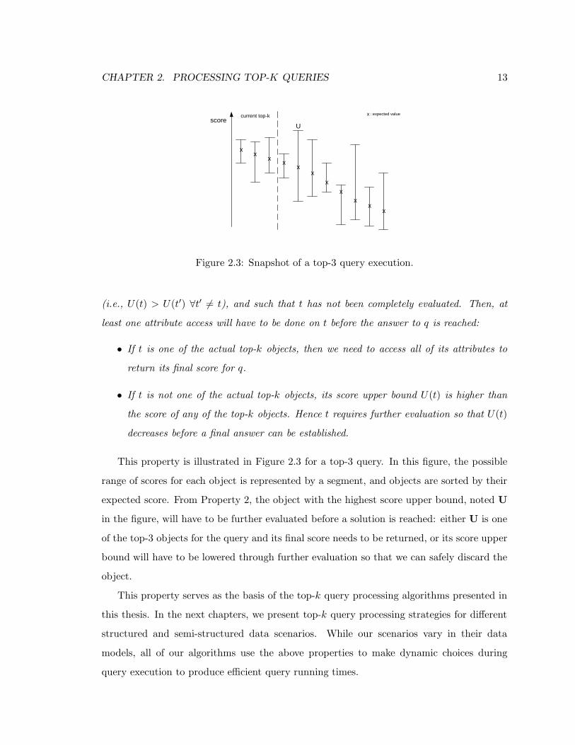
Figure 2.3: Snapshot of a top-3 query execution.
(i.e., U(t) > U(t′) ∀t′ 6= t), and such that t has not been completely evaluated. Then, at
least one attribute access will have to be done on t before the answer to q is reached:
• If t is one of the actual top-k objects, then we need to access all of its attributes to
return its final score for q.
• If t is not one of the actual top-k objects, its score upper bound U(t) is higher than
the score of any of the top-k objects. Hence t requires further evaluation so that U(t)
decreases before a final answer can be established.
This property is illustrated in Figure 2.3 for a top-3 query. In this figure, the possible
range of scores for each object is represented by a segment, and objects are sorted by their
expected score. From Property 2, the object with the highest score upper bound, noted U
in the figure, will have to be further evaluated before a solution is reached: either U is one
of the top-3 objects for the query and its final score needs to be returned, or its score upper
bound will have to be lowered through further evaluation so that we can safely discard the
object.
This property serves as the basis of the top-k query processing algorithms presented in
this thesis. In the next chapters, we present top-k query processing strategies for different
structured and semi-structured data scenarios. While our scenarios vary in their data
models, all of our algorithms use the above properties to make dynamic choices during
query execution to produce efficient query running times.
Chapter 3 14
Chapter 3
Sequential Top-k Query Processing
Strategies over Web-Accessible
Structured Data
In Chapter 2, we introduced our top-k query model, and presented object score properties
that we can exploit to produce efficient top-k query executions. In this chapter, we focus on
an important web application scenario and define efficient top-k query processing algorithms
for this scenario.
In our web application scenario, data objects are only available through remote, au-
tonomous web sources, exhibiting a variety of access interfaces and constraints as illustrated
in the example below.
Example 1 (cont.): Consider our restaurant example from Chapter 2. Each restaurant
attribute in this example might be available only through remote calls to external web sources:
the Rating attribute might be available through the Zagat-Review web site1, which, given an
individual restaurant name, returns its food rating as a number between 1 and 30 (“random
access”). This site might also return a list of all restaurants ordered by their food rating
(“sorted access”). Similarly, the Price attribute might be available through the New York
1http://www.zagat.com
CHAPTER 3. SEQUENTIAL TOP-K QUERY PROCESSING STRATEGIES 15
Times’s NYT-Review web site2. Finally, the scoring associated with the Address attribute
might be handled by the MapQuest web site, which returns the distance (in miles) between
the restaurant and the user addresses.
During query processing, the remote web sources have to be queried (or probed) repeat-
edly for a potentially large set of candidate objects. In our restaurant example, a possible
query processing strategy is to start with the Zagat-Review source, which supports sorted
access, to identify a set of candidate restaurants to explore further. This source returns a
rank of restaurants in decreasing order of food rating. To compute the final score for each
restaurant and identify the top-10 matches for our query, we then obtain the proximity be-
tween each restaurant and the user-specified address by querying MapQuest, and check the
average dinner price for each restaurant individually at the NYT-Review source. Hence, we
interact with three autonomous sources and repeatedly query them for a potentially large
set of candidate restaurants.
Processing top-k queries efficiently in such a scenario is challenging, as web sources ex-
hibit diverse probing costs and access interfaces. By considering the peculiarities of the
sources and potentially designing object-specific query execution plans, we design adap-
tive algorithms, based on the properties from Section 2.2, that efficiently prune useless
objects and produce significantly more efficient query executions than previously existing
algorithms, which select “global” query execution plans.
In this chapter, we make the following contributions:
• A data model that captures web source interfaces and probing costs.
• Some natural improvements to an existing top-k query processing strategy, TA [FLN01],
to decrease its query processing time.
• An efficient sequential top-k query processing algorithm that interleaves sorted and
random accesses during query processing and schedules random accesses at a fine-
granularity per-object level.
2http://www.nytoday.com

CHAPTER 3. SEQUENTIAL TOP-K QUERY PROCESSING STRATEGIES 16
• A thorough, extensive experimental evaluation of the new algorithms using real and
local data sets, and for a wide range of query parameters.
The rest of this chapter is organized as follows. First, we present our data model
in Section 3.1. Then, in Section 3.2, we discuss and improve on an existing top-k query
processing strategy. In Section 3.3, we present an efficient sequential top-k query processing
technique. In Section 3.4, we report on an extensive experimental evaluation of our strategy.
Finally, we conclude this chapter in Section 3.5. This chapter is based on work that has
been published in [BGM02, MBG04].
3.1 Data Model
In our web application scenario, data is accessed through probes to web sources, which
exhibit a variety of interfaces and access costs. In this section we refine the data and query
model of Chapter 2 and instantiate it to our web scenario. In this scenario, the object
attributes are handled and provided by autonomous sources accessible over the web with
a variety of interfaces. For instance, the Price attribute in Example 1 is provided by the
NYT-Review web site and can be accessed only by querying this site’s web interface3. We
distinguish between three types of sources based on their access interface:
Definition 1: [Source Types] Consider an attribute Ai and a top-k query q. Assume
further that Ai is handled by a source S. We say that S is an S-Source if we can obtain
from S a list of objects sorted in descending order of ScoreAiby (repeated) invocation of a
getNext(S, q) probe interface. Alternatively, assume that Ai is handled by a source R that
only returns scoring information when prompted about individual objects. In this case, we
say that R is an R-Source. R provides random access on Ai through a getScore(R, q, t)
probe interface, where t is a set of attribute values that identify an object in question. (As
a small variation, sometimes an R-Source will return the actual attribute Ai value for an
3Of course, in some cases we might be able to download all this remote information and cache it locally
with the query processor. However, this will not be possible for legal or technical reasons for some other
sources, or might lead to highly inaccurate or outdated information.

CHAPTER 3. SEQUENTIAL TOP-K QUERY PROCESSING STRATEGIES 17
object, rather than its associated score.) Finally, we say that a source that provides both
sorted and random access is an SR-Source.
Example 1 (cont.): In our restaurant example, attribute Rating is associated with the
Zagat-Review web site. This site provides both a list of restaurants sorted by their rating
(sorted access), and the rating of a specific restaurant given its name (random access).
Hence, Zagat-Review is an SR-Source. In contrast, Address is handled by the MapQuest
web site, which returns the distance between the restaurant address and the user-specified
address. Hence, MapQuest is an R-Source.
To define top-k query processing strategies over the three source types above, we need
to consider the cost that accessing such sources entails:
Definition 2: [Access Costs] Consider a source R that provides a random-access inter-
face, and a top-k query. We refer to the average time that it takes R to return the score
for a given object as tR(R). (tR stands for “random-access time.”) Similarly, consider a
source S that provides a sorted-access interface. We refer to the average time that it takes
S to return the top object for the query for the associated attribute as tS(S). (tS stands
for “sorted-access time.”) We make the simplifying assumption that successive invocations
of the getNext interface also take time tS(S) on average.
We make a number of assumptions in our presentation. The top-k evaluation strategies
that we consider do not allow for “wild guesses” [FLN01]: an object must be “discovered”
under sorted access before it can be probed using random access. Therefore, we need to
have at least one source with sorted access capabilities to discover new objects. We consider
nsr SR-Sources D1, . . ., Dnsr (nsr ≥ 1) and nr R-Sources Dnsr+1, . . ., Dn (nr ≥ 0), where
n = nsr + nr is the total number of sources. A scenario with several S-Sources (with no
random-access interface) is problematic: to return the top-k objects for a query together
with their scores, as required by our query model (Chapter 2), we might have to access all
objects in some of the S-Sources to retrieve the corresponding attribute scores for the top-k
objects. This can be extremely expensive in practice. Fagin et al. [FLN01] presented the
NRA algorithm to deal with multiple S-Sources; however, NRA only identifies the top-k
objects and does not compute their final scores.

CHAPTER 3. SEQUENTIAL TOP-K QUERY PROCESSING STRATEGIES 18
We refer to the set of all objects available through the sources as the Objects set. Addi-
tionally, we assume that all sources D1, . . . , Dn “know about” all objects in Objects. In other
words, given a query q and an object t ∈ Objects, we can obtain the score corresponding to q
and t for attribute Ai, for all i = 1, . . . , n. Of course, this is a simplifying assumption that is
likely not to hold in practice, where each source might be autonomous and not coordinated
in any way with the other sources. For instance, in our running example the NYT-Review
site might not have reviewed a specific restaurant, and hence it will not be able to return
a score for the Price attribute for such a restaurant. In this case, we simply use a default
value for t’s score for the missing attributes.
In this chapter, we focus on sequential top-k query processing strategies. In a sequential
setting, during query processing, we can have at most one outstanding (random- or sorted-
access) probe at any given time. When a probe completes, a sequential strategy chooses
either to perform sorted access on a source to potentially obtain unseen objects, or to pick
an already seen object, together with a source for which the object has not been probed,
and perform a random-access probe on the source to get the corresponding score for the
object.
3.2 An Existing Top-k Strategy
We now review and extend an existing algorithm to process top-k queries over sources
that provide sorted and random access interfaces. Specifically, in Section 3.2.1 we discuss
Fagin et al.’s TA algorithm [FLN01], and then propose improvements over this algorithm
in Section 3.2.2.
3.2.1 The TA Algorithm
Fagin et al. [FLN01] presented the TA algorithm for processing top-k queries over SR-Sources.
We adapted this algorithm in [BGM02] and introduced the TA-Adapt algorithm, which
handles one SR-Source and any number of R-Sources. Fagin et al. [FLN03] generalized
TA-Adapt to handle any number of SR-Sources and R-Sources. Their resulting algorithm,
TAz, is summarized in Figure 3.1.
CHAPTER 3. SEQUENTIAL TOP-K QUERY PROCESSING STRATEGIES 19
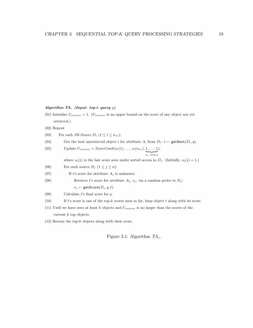
Algorithm TAz (Input: top-k query q)
(01) Initialize Uunseen = 1. (Uunseen is an upper bound on the score of any object not yet
retrieved.)
(02) Repeat
(03) For each SR-Source Di (1 ≤ i ≤ nsr):
(04) Get the best unretrieved object t for attribute Ai from Di: t← getNext(Di, q).
(05) Update Uunseen = ScoreComb(s`(1), . . . , s`(nsr), 1, . . . , 1| {z }
nr times
),
where s`(j) is the last score seen under sorted access in Dj . (Initially, s`(j) = 1.)
(06) For each source Dj (1 ≤ j ≤ n):
(07) If t’s score for attribute Aj is unknown:
(08) Retrieve t’s score for attribute Aj , sj , via a random probe to Dj :
sj ← getScore(Dj , q, t).
(09) Calculate t’s final score for q.
(10) If t’s score is one of the top-k scores seen so far, keep object t along with its score.
(11) Until we have seen at least k objects and Uunseen is no larger than the scores of the
current k top objects.
(12) Return the top-k objects along with their score.
Figure 3.1: Algorithm TAz.
CHAPTER 3. SEQUENTIAL TOP-K QUERY PROCESSING STRATEGIES 20
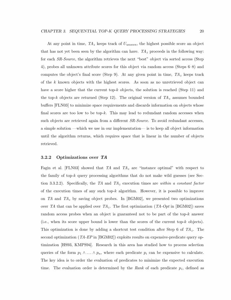
At any point in time, TAz keeps track of Uunseen, the highest possible score an object
that has not yet been seen by the algorithm can have. TAz proceeds in the following way:
for each SR-Source, the algorithm retrieves the next “best” object via sorted access (Step
4), probes all unknown attribute scores for this object via random access (Steps 6–8) and
computes the object’s final score (Step 9). At any given point in time, TAz keeps track
of the k known objects with the highest scores. As soon as no unretrieved object can
have a score higher that the current top-k objects, the solution is reached (Step 11) and
the top-k objects are returned (Step 12). The original version of TAz assumes bounded
buffers [FLN03] to minimize space requirements and discards information on objects whose
final scores are too low to be top-k. This may lead to redundant random accesses when
such objects are retrieved again from a different SR-Source. To avoid redundant accesses,
a simple solution —which we use in our implementation— is to keep all object information
until the algorithm returns, which requires space that is linear in the number of objects
retrieved.
3.2.2 Optimizations over TA
Fagin et al. [FLN03] showed that TA and TAz are “instance optimal” with respect to
the family of top-k query processing algorithms that do not make wild guesses (see Sec-
tion 3.3.2.2). Specifically, the TA and TAz execution times are within a constant factor
of the execution times of any such top-k algorithm. However, it is possible to improve
on TA and TAz by saving object probes. In [BGM02], we presented two optimizations
over TA that can be applied over TAz. The first optimization (TA-Opt in [BGM02]) saves
random access probes when an object is guaranteed not to be part of the top-k answer
(i.e., when its score upper bound is lower than the scores of the current top-k objects).
This optimization is done by adding a shortcut test condition after Step 6 of TAz. The
second optimization (TA-EP in [BGM02]) exploits results on expensive-predicate query op-
timization [HS93, KMPS94]. Research in this area has studied how to process selection
queries of the form p1 ∧ . . . ∧ pn, where each predicate pi can be expensive to calculate.
The key idea is to order the evaluation of predicates to minimize the expected execution
time. The evaluation order is determined by the Rank of each predicate pi, defined as

CHAPTER 3. SEQUENTIAL TOP-K QUERY PROCESSING STRATEGIES 21
Algorithm TAz-EP (Input: top-k query q)
(01) Initialize Uunseen = 1. (Uunseen is an upper bound on the score of any object not yet
retrieved.)
(02) Repeat
(03) For each SR-Source Di (1 ≤ i ≤ nsr):
(04) Get the best unretrieved object t for attribute Ai from Di: t← getNext(Di, q).
(05) Update Uunseen = ScoreComb(s`(1), . . . , s`(nsr), 1, . . . , 1| {z }
nr times
),
where s`(j) is the last score seen under sorted access in Dj . (Initially, s`(j) = 1.)
(06) For each source Dj (1 ≤ j ≤ n) in decreasing order of Rank(Dj) :
(07) If U(t) is less than or equal to the score of k objects, skip to (11).
(08) If t’s score for attribute Aj is unknown:
(09) Retrieve t’s score for attribute Aj , sj , via a random probe to Dj :
sj ← getScore(Dj , q, t).
(10) Calculate t’s final score for q.
(11) If we probed t completely and t’s score is one of the top-k scores, keep object t along
with its score.
(12) Until we have seen at least k objects and Uunseen is no larger than the scores of the current
k top objects.
(13) Return the top-k objects along with their score.
Figure 3.2: Algorithm TAz-EP.
Rank(pi) = 1−selectivity(pi)cost-per-object(pi)
, where selectivity(pi) is the fraction of the objects that are
estimated to satisfy pi, and cost-per-object(pi) is the average time to evaluate pi over an
object. We can adapt this idea to our framework as follows.
Let w1, . . . , wn be the weights of the sources D1, . . . , Dn in the scoring function ScoreComb .
If e(Ai) is the expected score of a randomly picked object for source Ri, the expected
decrease of U(t) after probing source Ri for object t is δi = wi · (1 − e(Ai)). We sort
the sources in decreasing order of their Rank, where Rank for a source Ri is defined as
Rank(Ri) = δi
tR(Ri). Thus, we favor fast sources that might have a large impact on the final
score of an object; these sources are likely to substantially change the value of U(t) fast.
We combine these two optimizations to define the TAz-EP algorithm (Figure 3.2). The
first optimization appears in Steps 7 and 11. The second optimization appears in Step 6.

CHAPTER 3. SEQUENTIAL TOP-K QUERY PROCESSING STRATEGIES 22
3.3 The Sequential Upper Algorithm
We now present a top-k query processing strategy that we call Upper, variants of which
we introduced in [BGM02] and [MBG04]. Our original formulation of Upper was for a
restricted scenario of only one SR-Source and any number of R-Sources. In [MBG04], we
relaxed this restriction to allow for any number of SR-Sources and R-Sources. Unlike TAz,
which completely probes each object immediately after the object is identified, Upper allows
for more flexible probe schedules in which sorted and random accesses can be interleaved
even when some objects have only been partially probed. When a probe completes, Upper
decides whether to perform a sorted-access probe on a source to get new objects, or to
perform the “most promising” random-access probe on the “most promising” object that
has already been retrieved via sorted access.
The Upper algorithm is detailed in Figure 3.3. Exploiting Property 2 from Section 2.2.2,
Upper chooses to probe the object with the highest score upper bound, since this object will
have to be probed at least once before a top-k solution can be reached. If the score upper
bound of unretrieved objects is higher than the highest score upper bound of the retrieved
objects, Upper chooses to retrieve a new object via sorted access. In this case, Upper has to
choose which SR-Source to access. This can be decided in several ways. A simple approach
that works well in practice is to use a round-robin algorithm (Step 6).
3.3.1 Selecting the Best Source
After Upper picks an object to probe, the choice of source to probe for the object (Step
14) is handled by the SelectBestSource function, and is influenced by a number of factors:
the cost of the random access probes, the weights of the corresponding attributes in the
scoring function (or the ranking function itself if we consider a scoring function different
than weighted sum), and the expected attribute scores.
The SelectBestSource function chooses the best source with which to probe object tH
next. (Object tH is picked in Step 3.) This choice should depend on whether tH is one of the
top-k objects or not. To define this function, we would then need to know the k-th highest
actual score scorek among all objects in Objects. Of course, Upper does not know the actual
CHAPTER 3. SEQUENTIAL TOP-K QUERY PROCESSING STRATEGIES 23
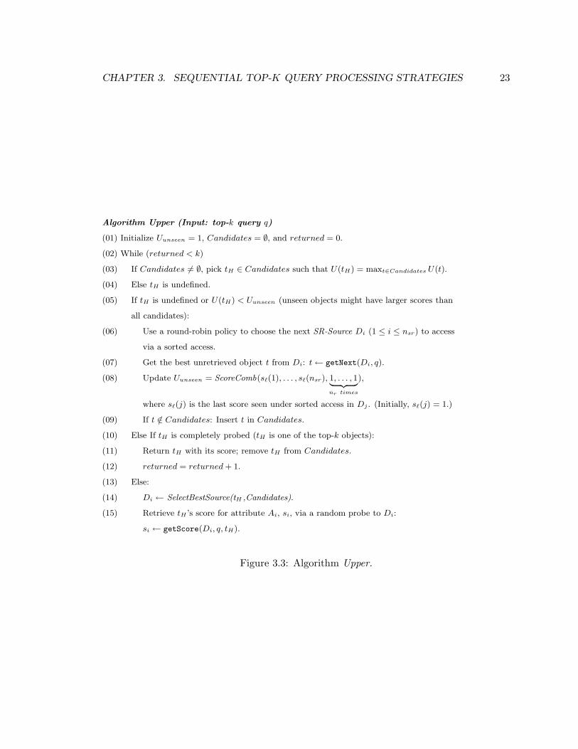
Algorithm Upper (Input: top-k query q)
(01) Initialize Uunseen = 1, Candidates = ∅, and returned = 0.
(02) While (returned < k)
(03) If Candidates 6= ∅, pick tH ∈ Candidates such that U(tH) = maxt∈Candidates U(t).
(04) Else tH is undefined.
(05) If tH is undefined or U(tH) < Uunseen (unseen objects might have larger scores than
all candidates):
(06) Use a round-robin policy to choose the next SR-Source Di (1 ≤ i ≤ nsr) to access
via a sorted access.
(07) Get the best unretrieved object t from Di: t← getNext(Di, q).
(08) Update Uunseen = ScoreComb(s`(1), . . . , s`(nsr), 1, . . . , 1| {z }
nr times
),
where s`(j) is the last score seen under sorted access in Dj . (Initially, s`(j) = 1.)
(09) If t /∈ Candidates: Insert t in Candidates.
(10) Else If tH is completely probed (tH is one of the top-k objects):
(11) Return tH with its score; remove tH from Candidates.
(12) returned = returned + 1.
(13) Else:
(14) Di ← SelectBestSource(tH ,Candidates).
(15) Retrieve tH ’s score for attribute Ai, si, via a random probe to Di:
si ← getScore(Di, q, tH).
Figure 3.3: Algorithm Upper.

CHAPTER 3. SEQUENTIAL TOP-K QUERY PROCESSING STRATEGIES 24
object scores a priori, so it relies on expected scores to make its choices and estimates the
value scorek (i.e., the k-th top score) using score′k, the k-th largest expected object score.
(We define score′k = 0 if we have retrieved fewer than k objects.) We considered several
implementations of the SelectBestSource function [GMB02], such as a greedy approach, or
considering the best subset of sources for object tH that is expected to decrease U(tH)
below score′k (this implementation of SelectBestSource was presented in [BGM02]). Our
experimental evaluation [GMB02] shows that using the “non-redundant sources” approach
that we discuss below for SelectBestSource results in the best performance, so we only focus
on this version of the function in the remainder of this chapter, for conciseness.
Our implementation of SelectBestSource picks the next source to probe for object tH by
first deciding whether tH is likely to be one of the top-k objects or not:
• Case 1: E(tH) < score′k. In this case, tH is not expected to be one of the top-k
objects. To decide what source to probe next for tH , we favor sources that can have a
high “impact” (i.e., that can sufficiently reduce the score of tH so that we can discard
tH) while being efficient (i.e., with a relatively low value for tR). More specifically,
∆ = U(tH)−score′k is the amount by which we need to decrease U(tH) to “prove” that
tH is not one of the top-k answers. In other words, it does not really matter how large
the decrease of U(tH) is beyond ∆ when choosing the best probe for tH . Note that it
is always the case that ∆ ≥ 0: from the choice of tH , it follows that U(tH) ≥ score′k.
To see why, suppose that U(tH) < score′k. Then U(tH) < E(t) ≤ U(t) for k objects t,
from the definition of score′k. But U(tH) is highest among the objects in Candidates,
which would imply that the k objects t such that U(t) > U(tH) had already been
removed from Candidates and output as top-k objects. And this is not possible since
the final query result has not been reached (returned < k; see Step 2). Also, the
expected decrease of U(tH) after probing source Ri is given by δi = wi · (1 − e(Ai)),
where wi is the weight of attribute Ai in the query (Chapter 2) and e(Ai) is the
expected score for attribute Ai. Then, the ratio:
Rank(Ri) =Min{∆, δi}
tR(Ri)
is a good indicator of the “efficiency” of source Ri: a large value of this ratio indicates
CHAPTER 3. SEQUENTIAL TOP-K QUERY PROCESSING STRATEGIES 25
that we can reduce the value of U(tH) by a sufficiently large amount (i.e., Min {∆, δi})
relative to the time that the associated probe requires (i.e., tR(Ri)).4
Interestingly, while choosing the source with the highest rank value is efficient, it
sometimes results in provably sub-optimal choices, as illustrated in the following ex-
ample.
Example 2: Consider an object t and two R-Sources R1 and R2, with access times
tR(R1)=1 and tR(R2)=10, and query weights w1=0.1 and w2=0.9. Assume that
score′k=0.5 and U(t) = 0.9, so the amount by which we need to decrease t to “prove”
it is not one of the top answers is expected to be ∆ = 0.9 − 0.5 = 0.4. If we assume
that e(A1)=e(A2)=0.5, we would choose source R1 (with rank Min{0.4,0.05}1 = 0.05)
over source R2 (with rank Min{0.4,0.45}10 = 0.04). However, we know that we will need
to eventually lower U(t) below score′k=0.5, and that R1 can only decrease U(t) by 0.1
to 0.8, since w1=0.1. Therefore, in subsequent iterations, source R2 would need to be
probed anyway. In contrast, if we start with source R2, we might decrease U(t) below
score′k = 0.5 with only one probe, thus avoiding a probe to source R1 for t.
The previous example shows that, for a particular object t, a source Ri can be “redun-
dant” independently of its rank Min{∆, δi}/tR(Ri). Therefore, such a source should
not be probed for t before the “non-redundant” sources. The set of redundant sources
for an object is not static, but rather depends on the execution state of the algorithm.
(In the example above, if score′k = 0.89, there are no redundant sources for object
t.) To identify the subset of non-redundant available sources for object tH , we let
∆ = U(tH)− score′k as above and let R = {R1, . . . , Rm} be the set of sources not yet
probed for tH . If ∆ = 0, all sources are considered not to be redundant. Otherwise, if
4SelectBestSource might need to be modified to handle scoring functions other than the weighted-sum
function. In particular, for functions where the final object scores cannot be in general approximated or
usefully bounded unless all input values are known (e.g., as is the case for the min function), a per-object
scheduling strategy is not necessary. In such cases, the probe history of an object does not impact source
choice and so, the SelectBestSource function should make decisions at a higher level of granularity (e.g., by
ordering sources based on source access time).

CHAPTER 3. SEQUENTIAL TOP-K QUERY PROCESSING STRATEGIES 26
∆ > 0 we say that source Ri is redundant for object tH at a given step of the probing
process if ∀Y ⊆ R − {Ri} : If wi +∑
j:Rj∈Y wj ≥ ∆ then∑
j:Rj∈Y wj ≥ ∆ (i.e., for
every possible choice of sources {Ri} ∪ Y that can decrease U(tH) to score′k or lower,
Y by itself can also do it). By negating the predicate above, replacing the implication
with the equivalent disjunction, and manipulating the resulting predicate, we obtain
the following test to identify non-redundant sources: Ri is non-redundant if and only
if ∃Y ⊆ R − {Ri} : ∆ − wi ≤∑
j:Rj∈Y wj < ∆. It is not difficult to prove that, for
any possible assignment of values to wi and ∆ > 0, there is always at least one avail-
able non-redundant source. Therefore, after identifying the subset of non-redundant
sources, our SelectBestSource function returns the non-redundant source for object tH
with the maximum rank Min{∆,δi}tR(Ri)
if ∆ > 0. If ∆ = 0, all sources have the same Rank
value, and we pick the source with the fastest random-access time for the query.
• Case 2: E(tH) ≥ score′k. In this case, tH is expected to be one of the top-k objects,
and so we will need to probe tH completely. Therefore all sources for which tH has
not been probed are non-redundant and SelectBestSource returns the not-yet-probed
source with the highest δi
tR(Ri)ratio.
In summary, when a probe completes, Upper can either (a) perform a sorted-access
probe on a source if the unseen objects have the highest score upper bound (Steps 5–9), or
(b) select both an object and a source to probe next (Steps 13–15), guided in both cases by
Property 2. In addition, Upper can return results as they are produced, rather than having
to wait for all top-k results to be known before producing the final answer (Steps 10–12).
3.3.2 Cost Analysis
We now discuss the efficiency of the various algorithms. Specifically, Section 3.3.2.1 analyzes
the number of sorted accesses that each algorithm requires, and Section 3.3.2.2 discusses
the optimality of Upper.
3.3.2.1 Counting Sorted Accesses
Interestingly, Upper and TAz behave in an identical manner with respect to sorted accesses:
CHAPTER 3. SEQUENTIAL TOP-K QUERY PROCESSING STRATEGIES 27
Lemma 1: Consider a top-k query q over multiple SR-Sources and R-Sources. Then, Upper
and all variations of TAz perform the same number of sorted accesses when processing q.
Proof 1: We note that the choice of sorted-access sources in both TAz and Upper follows
the same fixed round-robin strategy, which is independent of the input (see Step 3 for TAz
in Figure 3.1 and Step 6 for Upper in Figure 3.3). Therefore, after Upper or TAz perform
some equal number of sorted accesses, the value of Uunseen is the same for both algorithms.
Consider the execution of both TAz and Upper after both algorithms have retrieved the same
set Retrieved of objects, with |Retrieved| ≥ k. (Naturally, TAz and Upper need to retrieve
at least k objects via sorted access to output the top-k solution.)
• If TAz decides to retrieve a new object after processing the objects in Retrieved, then
it holds that Uunseen > Score(q,m), where m is the object in Retrieved with the k-th
largest score. Suppose that the execution of Upper finishes without retrieving any new
object beyond those in Retrieved, and let m′ be the k-th object output as Upper’s result
for q. Since m′ was also retrieved by TAz, and because of the choice of m, it holds
that Score(q,m) = Score(q,m′). Then Score(q,m′) < Uunseen and hence Upper could
never have output this object as part of the query result (see Step 5 in Figure 3.3),
contradicting the choice of m′. Therefore Upper also needs to retrieve a new object,
just as TAz does.
• If Upper decides to retrieve a new object after processing the objects in Retrieved, then
it holds that Upper output fewer than k objects from Retrieved as part of the query
result, and that U(t) < Uunseen for each object t ∈ Retrieved not yet output (see
Step 5 in Figure 3.3). Then, since Score(q, t) ≤ U(t) for each object t, it follows that
Score(q,m) < Uunseen, where m is the object in Retrieved with the k-th largest actual
score for q. Therefore, from Step 11 in Figure 3.1 it follows that TAz also needs to
retrieve a new object, just as Upper does.
2
Interestingly, since TAz performs all random accesses for the objects considered, Upper
never performs more random accesses than TAz does.

CHAPTER 3. SEQUENTIAL TOP-K QUERY PROCESSING STRATEGIES 28
3.3.2.2 Instance Optimality
As presented in [FLN03], TAz is “instance optimal,” where the definition of “instance
optimality” —slightly adapted from [FLN03] to match our terminology— is:
Definition 3 [Instance Optimality] Let A be a class of algorithms and D be a class
of source instances. An algorithm B ∈ A is instance optimal over A and D if there are
constants c and c′ such that for every A ∈ A and D ∈ D we have that cost(B,D) ≤
c · cost(A,D) + c′, where cost(a,D) is, in our context, the combined sorted- and random-
access time required by algorithm a over the sources in D.
An interesting observation is that the number of random accesses in TAz is an upper
bound on the number of random accesses in TAz-EP: TAz-EP is an optimization over TAz
aimed at reducing the number of random accesses. The shortcuts used in TAz-EP are only
used to discard objects sooner than in TAz and do not affect the number of sorted accesses
performed by the algorithm. Also, as explained in the previous section, Upper performs no
more sorted or random accesses than TAz does. Hence, the TAz “instance optimality” also
applies to the TAz-EP and Upper algorithms. Therefore, the experimental section of the
chapter (Section 3.4), in which we compare the TAz and Upper algorithms, will evaluate
the algorithms with real-world and local data to measure their “absolute” efficiency (they
are all “instance optimal”).
3.4 Experimental Results
We performed an extensive experimental evaluation of Upper. In this section, we first
discuss our implementation choices and evaluation settings (Section 3.4.1), then report
results over real and synthetic data sets (Section 3.4.2), compare Upper with MPro [CH02],
a competing algorithm that does not make per-object scheduling choices (Section 3.4.3),
and present results over real web sources (Section 3.4.4)

CHAPTER 3. SEQUENTIAL TOP-K QUERY PROCESSING STRATEGIES 29
3.4.1 Implementation
In this section, we first present the query processing techniques used in our experimental
evaluation (Section 3.4.1.1) and discuss data structures that we use to implement these
query processing strategies (Section 3.4.1.2). We also define the local (Section 3.4.1.3) and
real data sets (Section 3.4.1.4) that we use for the experimental evaluation of the various
techniques, as well as the prototype that we implemented for our experiments over real
web-accessible sources (Section 3.4.4). Finally, we discuss the metrics and other settings
that we use in our experimental evaluation (Section 3.4.1.5) .
3.4.1.1 Techniques
We compare the performance of Upper (Section 3.3) with that of TAz-EP (Section 3.2.1).
In addition, we consider MPro, an algorithm presented by Chang and Hwang [CH02] to
optimize the execution of expensive predicates for top-k queries, rather than for our web-
source scenario. MPro is more general than our techniques in that it targets a wider range
of scenarios: local expensive predicates, external expensive predicates, arbitrary monotonic
scoring functions, and joins. Their “probes” are typically not as expensive as our web-
source accesses, hence the need for faster probe scheduling. Unlike our Upper technique
(Section 3.3), MPro defines a fixed schedule of accesses to R-Sources during an initial
object-sampling step, and thus selects which object to probe next during query execution
but avoids source selection on a per-object basis.
Upper is a technique in which source probes are scheduled at a fine object-level granu-
larity, and where probes on different objects can be interleaved (see Table 3.1). In contrast,
TAz-EP is a technique in which source probes are scheduled at a coarse query-level granular-
ity, and where each object is fully processed before probes on a different object can proceed.
MPro is an example of a technique with interleaving of probes on different objects and with
query-level probe scheduling. (We evaluate MPro experimentally in Section 3.4.2.3, where
we consider a scenario in which object sampling —as required by MPro— is possible. We
also defer the discussion of the Upper-Sample technique outlined in Table 3.1 until that
section.) MPro-EP is an instantiation of the MPro algorithm with a different source-order
criterion. Specifically, MPro-EP departs from the original MPro algorithm in that it does

CHAPTER 3. SEQUENTIAL TOP-K QUERY PROCESSING STRATEGIES 30
Per-Query Scheduling Per-Object Scheduling
of Probes of Probes
No Interleaving of TAz-EP TAz-SelectBestSource
Probes across Objects
Interleaving No Sampling MPro-EP Upper
of Probes Available
across Objects Sampling MPro Upper-Sample
Available
Table 3.1: “Dimensions” to characterize sequential query processing algorithms.
not rely on object sampling and orders sources by their Rank values as defined in Sec-
tion 3.2.2. Note that MPro-EP can also be regarded as a modification of Upper for which
the SelectBestSource function always considers each source’s object-independent Rank value
as defined in Section 3.2.2 when deciding what source to pick for a given object.
The “dimensions” outlined in Table 3.1 suggest an additional technique. This technique,
denoted as TAz-SelectBestSource in Table 3.1, is similar to TAz-EP in that it does not
interleave probes on multiple objects. However, the schedule of probes on each object is not
fixed, but rather is influenced by the returned probe scores and determined dynamically
using Upper’s SelectBestSource function. For conciseness, we do not report experimental
figures for this technique, since it results in only minor time savings over the simpler TAz-EP
algorithm. Similarly, we do not consider variations of TAz-EP and TAz-SelectBestSource
that exploit sampling-derived information.
By comparing MPro-EP and TAz-EP, our experiments help quantify the saving in prob-
ing time that is due to the interleaving of object probes. By comparing MPro-EP and Upper,
our experiments help understand the impact of the relatively expensive per-object schedul-
ing on query processing efficiency.
CHAPTER 3. SEQUENTIAL TOP-K QUERY PROCESSING STRATEGIES 31
3.4.1.2 Supporting Data Structures
Our algorithms keep track of the objects retrieved and their partial score information in a
hash table indexed by the object ids. For each object, we record the attribute scores returned
by the different sources (a special value is used when information about a particular source
is not yet available). For efficiency, we also incrementally maintain the score upper bounds
of each object. Finally, depending on the algorithm, each object is augmented with a small
number of pointers that help us to efficiently maintain the rank of each object in different
ordered lists (see [GMB02]). During the execution of the algorithms of Sections 3.4.1.1,
each object can be part of multiple sorted lists. As an example, Upper (Section 3.3) needs
to keep track of the object with the largest score upper bound (Step 3 in the algorithm in
Figure 3.3). The SelectBestSource function also needs to identify the object with the k-th
highest expected score. We implement each sorted list using heap-based priority queues,
which provide constant-time access to the first ranked element, and logarithmic-time inser-
tions and deletions. We additionally modified these standard priority queues to extract in
constant time the k-th ranked object in the list still with logarithmic-time insertions and
deletions.
3.4.1.3 Local Sources
We generate a number of local SR-Sources and R-Sources for our experiments. The attribute
values for each object are generated using one of the following distributions:
Uniform: Attributes are independent of each other and attribute values are uniformly
distributed (default setting).
Gaussian: Attributes are independent of each other and attribute values are generated
from five overlapping multidimensional Gaussian bells [PFTV93].
Zipfian: Attributes are independent of each other and attribute values are generated from
a Zipf function with 1,000 distinct values and Zipfian parameter z = 1. The 1,000 distinct
attribute values are generated randomly in the [0,1] range, and the i-th most frequent
attribute value appears f(i) = |Objects|/(iz ·∑1,000
j=1 1/jz) times.
Correlated: We divide sources into two groups and generate attribute values so that values

CHAPTER 3. SEQUENTIAL TOP-K QUERY PROCESSING STRATEGIES 32
k nsr nr |Objects| tR tS Data Sets
50 3 3 10,000 [1, 10] [0.1, 1] Uniform
Table 3.2: Default parameter values for experiments over local data.
from sources within the same group are correlated. In each group, the attribute values for
a “base” source are generated using a uniform distribution. The attribute values for the
other sources in a group are picked for an object from a short interval around the object’s
attribute value in the “base” source. Our default Correlated data set consists of two groups
of three sources each.
Mixed: Attributes are independent of each other. Sources are divided into three groups,
and the attribute values within each group are generated using the Uniform, Gaussian, and
Zipfian distributions, respectively.
Cover: To validate our techniques on real data distributions, we performed experiments
over the Cover data set, a six-dimensional projection of the CovType data set [HBM98],
used for predicting forest cover types from cartographic variables. The data contains infor-
mation about various wilderness areas. Specifically, we consider six attributes: elevation (in
meters), aspect (in degrees azimuth), slope (in degrees), horizontal distance to hydrology
(in meters), vertical distance to hydrology (in meters), and horizontal distance to roadways
(in meters). We extracted a database of 10,000 objects from the CovType data set.
For simplicity, we will refer to the these sources as the “local” sources, to indicate that
these are locally available sources under our control, as opposed to the real web sources
described next. For our experiments, we vary the number of SR-Sources nsr, the number of
R-Sources nr, the number of objects available through sorted access |Objects|, the random
access time tR(Di) for each source Di (a random value between 1 and 10), and the sorted
access time tS(Di) for each source Di (a random value between 0.1 and 1). Table 3.2
lists the default value for each parameter. Unless we specify otherwise, we use this default
setting.

CHAPTER 3. SEQUENTIAL TOP-K QUERY PROCESSING STRATEGIES 33
Source Attribute(s) Input
Verizon Yellow Pages (S) Distance type of cuisine, user address
Subway Navigator (R) SubwayTime restaurant address, user address
MapQuest (R) DrivingTime restaurant address, user address
AltaVista (R) Popularity free text with restaurant name
and address
Zagat Review (R) ZFood, ZService, restaurant name
ZDecor, ZPrice
NYT Review (R) TRating, TPrice restaurant name
Table 3.3: Real web-accessible sources used in the experimental evaluation.
3.4.1.4 Real Web-Accessible Sources
In addition to experiments over the “local” data sets above, we evaluated the algorithms
over real, autonomous web sources. For this, we implemented a prototype of the algorithms
to answer top-k queries about New York City restaurants. Our prototype is written in C++
and Python.
Users input a starting address and their desired type of cuisine (if any), together with
importance weights for the following R-Source attributes: SubwayTime (handled by the
SubwayNavigator site5), DrivingTime (handled by the MapQuest site), Popularity (handled
by the AltaVista search engine6; see below), ZFood, ZService, ZDecor, and ZPrice (handled
by the Zagat-Review web site), and TRating and TPrice (provided by the New York Times’s
NYT-Review web site). The Verizon Yellow Pages listing7, which for sorted access returns
restaurants of the user-specified type sorted by shortest distance from a given address, is
the only SR-Source. Table 3.3 summarizes these sources and their interfaces.
The Popularity attribute requires further explanation. We approximate the “popularity”
of a restaurant with the number of web pages that mention the restaurant, as reported by
the AltaVista search engine. (The idea of using web search engines as a “popularity oracle”
5http://www.subwaynavigator.com
6http://www.altavista.com
7http://www.superpages.com

CHAPTER 3. SEQUENTIAL TOP-K QUERY PROCESSING STRATEGIES 34
has been used before in the WSQ/DSQ system [GW00].) Consider, for example, restaurant
“Tavern on the Green,” which is one of the most popular restaurants in the United States.
As of the writing of this thesis, a query on AltaVista on “Tavern on the Green” AND “New
York” returns 82,100 hits. In contrast, the corresponding query for a much less popular
restaurant in New York City, “Caffe Taci” AND “New York,” returns only 470 hits. Of
course, the reported number of hits might inaccurately capture the actual number of pages
that talk about the restaurants in question, due to both false positives and false negatives.
Also, in rare cases web presence might not reflect actual “popularity.” However, anecdotal
observations indicate that search engines work well as coarse popularity oracles.
Attributes Distance, SubwayTime, DrivingTime, ZFood, ZService, ZDecor, and TRating
have “default” target values in the queries (e.g., a DrivingTime of 0 and a ZFood rating
of 30). The target value for Popularity is arbitrarily set to 100 hits, while the ZPrice and
TPrice target values are set to the least expensive value in the scale. In the default setting,
the weights of all six sources are equal.
Naturally, the real sources above do not fit our model of Section 3.1 perfectly. For
example, some of these sources return scores for multiple attributes simultaneously (e.g.,
as is the case for the Zagat-Review site). Also, as we mentioned before, information on a
restaurant might be missing in some sources (e.g., a restaurant might not have an entry at
the Zagat-Review site). In such a case, our system will give a default (expected) score of
0.5 to the score of the corresponding attribute.
In a real web environment, source access times are usually not fixed and depend on
several parameters such as network traffic or server load. Using a fixed approximation of
the source response time (such as an average of past response times) may result in degraded
performance since our algorithms use these times to choose what probe to do next.
To develop accurate adaptive estimates for the tR times, we adapt techniques for esti-
mating the round trip time of network packets. Specifically, TCP implementations use a
“smoothed” round trip time estimate (SRTT ) to predict future round trip times, computed
as follows:
SRTT i+1 = (α × SRTT i) + ((1 − α) × si)
where SRTT i+1 is the new estimate of the round trip time, SRTT i is the current estimate

CHAPTER 3. SEQUENTIAL TOP-K QUERY PROCESSING STRATEGIES 35
of the round trip time, si is the time taken by the last round trip sample, and α is a
constant between 0 and 1 that controls the sensitivity of the SRTT to changes. For good
performance, Mills [Mil83] recommends using two values for α: α = 15/16, when the last
sample time is lower than the estimate time (SRTT i), and α = 3/4, when the last sample
time is higher than the estimate. This makes the estimate more responsive to increases in
the source response time than to decreases. Our prototype keeps track of the response time
of probes to each R-Source Ri and adjusts the average access time for Ri, tR(Ri), using
the SRTT estimates above. Since the sorted accesses to the SR-Sources Si are decided
independently of their sorted-access times, we do not adjust tS(Si).
3.4.1.5 Evaluation Metrics and Other Experimental Settings
To understand the relative performance of the various top-k processing techniques over local
sources, we time the two main components of the algorithms:
• tprobes is the time spent accessing the remote sources, in “units” of time. (In Sec-
tion 3.4.2.2, we report results for different values —in msecs.— of this time unit.)
• tlocal is the time spent locally scheduling remote source accesses, in seconds.
While source access and local scheduling happen in parallel, it is revealing to analyze the
tprobes and tlocal times associated with the query processing techniques separately, since the
techniques that we consider differ significantly in the amount of local processing time that
they require. For the experiments over the real-web sources, we report the total query
execution time:
• ttotal is the total time spent executing a top-k query, in seconds, including both remote
source access and scheduling.
We also report the number of random probes issued by each technique:8
• |probes| is the total number of random probes issued during a top-k query execution.
8The number of sorted accesses is the same for all presented techniques (Section 3.3.2.1).

CHAPTER 3. SEQUENTIAL TOP-K QUERY PROCESSING STRATEGIES 36
For the local sources, unless we note otherwise we generate 100 queries randomly, with
attribute weights randomly picked in the [1,10] range. We report the average values of the
metrics for different settings of nsr, nr, |Objects|, and k for different attribute distributions.
We conducted experiments on 1.4Ghz 2Gb RAM machines running Red Hat Linux 7.1.
For the real web sources, we defined queries that ask for top French, Italian, and Japanese
restaurants in Manhattan, for users located in different addresses. Attribute weights are
arbitrarily picked from the [1,10] range for each query. We report the average ttotal value for
different queries. We conducted experiments on a 550Mhz 758MB RAM machine running
Red Hat Linux 7.1.
3.4.2 Experiments over Local Data
We now report results for the sequential techniques over the local data sets presented in
Section 3.4.1.3. We first report on the performance of the techniques in terms of probing
time in Section 3.4.2.1. Then, in Section 3.4.2.2, we compare the local processing time
needed by the different techniques. Finally, in Section 3.4.2.3, we study the effect of data
score distribution knowledge on the techniques.
3.4.2.1 Probing Time
In this section, we report on the probing time of the sequential techniques for a range of
query and local data set parameters.
Effect of the Attribute Value Distribution: Figure 3.4 reports results for the default
setting (Table 3.2), for various attribute value distributions. In all cases, Upper substantially
outperforms TAz-EP. The performance of MPro-EP is just slightly worse than that of Upper,
which suggests that the gain in probing time of Upper over TAz-EP mostly results from
interleaving probes on objects. Interestingly, while Upper has faster overall probing times
that MPro-EP, MPro-EP results in slightly fewer random accesses (e.g., for the Uniform
data set, Upper performed on average 11,342 random accesses and MPro-EP performed on
average 11,045 random accesses). For the Cover data set, which consists of real-world data,
the results are similar to those for the other data sets.
Effect of the Number of Objects Requested k: Figure 3.5 reports results for the

CHAPTER 3. SEQUENTIAL TOP-K QUERY PROCESSING STRATEGIES 37
0
10000
20000
30000
40000
50000
60000
70000
80000
90000
100000
Uniform Gaussian Zipfian Correlated Mixed Cover
t pro
bes
Upper MPro-EP TAz-EP
Figure 3.4: Performance of the different strategies for the default setting of the experiment
parameters, and for alternate attribute-value distributions.
default setting (Table 3.2) as a function of k. As k increases, the time needed by each
algorithm to return the top-k objects increases as well, since all techniques need to retrieve
and process more objects. Once again, the Upper strategy consistently outperforms TAz-
EP, with MPro-EP as a close second.
Effect of the Number of Sources n: Figure 3.6 reports results for the default set-
ting, as a function of the total number of sources n (half the sources are SR-Sources, half
are R-Sources). Not surprisingly, the tprobes time needed by all the algorithms increases
with the number of available sources. When we consider a single SR-Source and a single
R-Source, tprobes is the same for all algorithms. However, when more sources are available,
the differences between the techniques become more pronounced, with Upper and MPro-EP
consistently resulting in the best performance.
Effect of the Number of SR-Sources nsr: Figure 3.7 reports results for the default setting,
as a function of the total number of sources nsr (out of a total of six sources). The per-
formance of TAz-EP remains almost constant when we vary the number of SR-Sources. In
contrast, the performance of Upper and MPro-EP improves when the number of SR-Sources
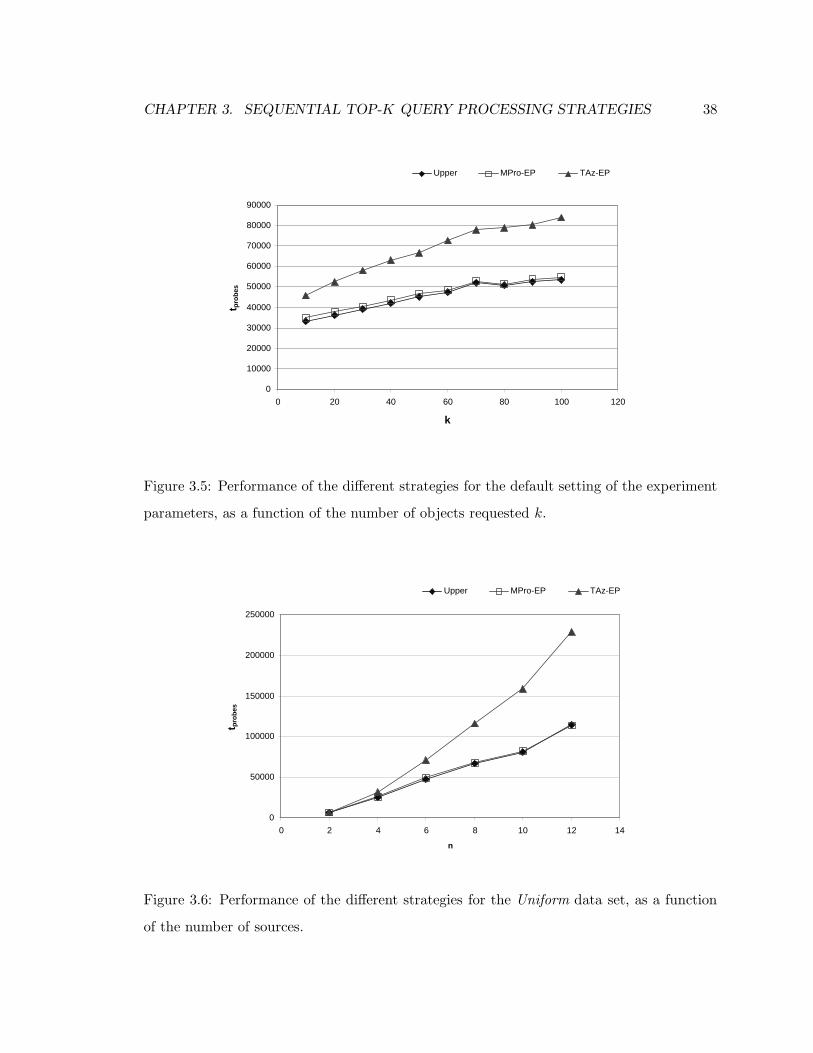
CHAPTER 3. SEQUENTIAL TOP-K QUERY PROCESSING STRATEGIES 38
0
10000
20000
30000
40000
50000
60000
70000
80000
90000
0 20 40 60 80 100 120
k
t pro
bes
Upper MPro-EP TAz-EP
Figure 3.5: Performance of the different strategies for the default setting of the experiment
parameters, as a function of the number of objects requested k.
0
50000
100000
150000
200000
250000
0 2 4 6 8 10 12 14
n
t pro
bes
Upper MPro-EP TAz-EP
Figure 3.6: Performance of the different strategies for the Uniform data set, as a function
of the number of sources.
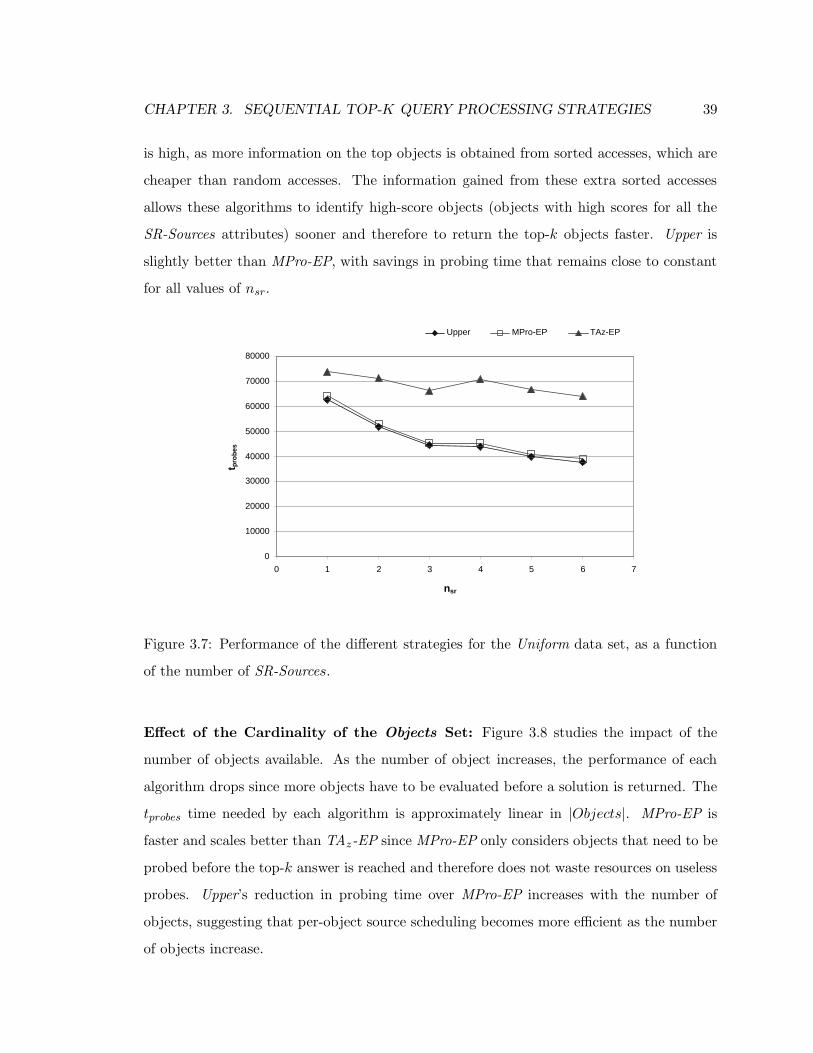
CHAPTER 3. SEQUENTIAL TOP-K QUERY PROCESSING STRATEGIES 39
is high, as more information on the top objects is obtained from sorted accesses, which are
cheaper than random accesses. The information gained from these extra sorted accesses
allows these algorithms to identify high-score objects (objects with high scores for all the
SR-Sources attributes) sooner and therefore to return the top-k objects faster. Upper is
slightly better than MPro-EP, with savings in probing time that remains close to constant
for all values of nsr.
0
10000
20000
30000
40000
50000
60000
70000
80000
0 1 2 3 4 5 6 7
n sr
t pro
bes
Upper MPro-EP TAz-EP
Figure 3.7: Performance of the different strategies for the Uniform data set, as a function
of the number of SR-Sources.
Effect of the Cardinality of the Objects Set: Figure 3.8 studies the impact of the
number of objects available. As the number of object increases, the performance of each
algorithm drops since more objects have to be evaluated before a solution is returned. The
tprobes time needed by each algorithm is approximately linear in |Objects|. MPro-EP is
faster and scales better than TAz-EP since MPro-EP only considers objects that need to be
probed before the top-k answer is reached and therefore does not waste resources on useless
probes. Upper’s reduction in probing time over MPro-EP increases with the number of
objects, suggesting that per-object source scheduling becomes more efficient as the number
of objects increase.

CHAPTER 3. SEQUENTIAL TOP-K QUERY PROCESSING STRATEGIES 40
0
50000
100000
150000
200000
250000
300000
350000
400000
450000
0 20000 40000 60000 80000 100000
|Objects|
t pro
bes
Upper MPro-EP TAz-EP
Figure 3.8: Performance of the different strategies for the Uniform data set, as a function
of the cardinality of Objects.
3.4.2.2 Local Processing Time
In the previous section, we showed that Upper and MPro-EP result in substantially fewer
random probes than TAz-EP. However, probe interleaving requires expensive computation
as object score information needs to be kept and sorted. In addition, Upper requires more
expensive probe scheduling than TAz-EP and MPro-EP do, so we now turn to studying the
effect of this local computation on overall performance. Interestingly, we show experimen-
tally that Upper results in considerably faster executions than TAz-EP, considering both
probing time and local execution time. Our experiments also show that Upper results in
slightly faster overall query execution times than MPro-EP.
Figure 3.9 shows the tlocal time for Upper, MPro-EP, and TAz-EP for the default setting
of the experiments in Table 3.2, and for varying number of objects. Not surprisingly, TAz-
EP is locally more efficient than Upper and MPro-EP. The additional local processing needed
by Upper and MPro-EP is spent maintaining object queues. (Both techniques need access
to the object with the largest score upper bound at different points in time.) In turn, Upper
is more expensive than MPro-EP because of two factors: (1) Upper schedules probes at the

CHAPTER 3. SEQUENTIAL TOP-K QUERY PROCESSING STRATEGIES 41
0
2
4
6
8
10
12
14
16
18
0 20000 40000 60000 80000 100000
|Objects|
t loca
l (i
n s
eco
nd
s)
Upper MPro-EP TAz-EP
Figure 3.9: The local processing time for Upper, MPro-EP, and TAz-EP, as a function of
the number of objects.
50
100
150
0.00001 0.0001 0.001 0.01 0.1 1 10
f (in seconds)
t tota
l (n
orm
aliz
ed w
ith
res
pec
t to
TA
z-E
P=1
00)
Upper MPro-EP TAz-EP
Figure 3.10: The total processing time for Upper, MPro-EP, and TAz-EP, as a function of
the time unit f.
CHAPTER 3. SEQUENTIAL TOP-K QUERY PROCESSING STRATEGIES 42
object level, while MPro-EP does so at a coarser query level, and (2) unlike MPro-EP, Upper
needs fast access to the object with the k-th largest expected score, for which the modified
priority queue mentioned in Section 3.4.1.2 needs to be maintained. Interestingly, the second
factor above accounts for most of the difference in execution time between Upper and MPro-
EP according to our experiments. If random accesses are fast, then the extra processing
time required by Upper is likely not to pay off. In contrast, for real web sources, with high
latencies, the extra local work is likely to result in faster overall executions. To understand
this interaction between local processing time and random-access time, we vary the absolute
value of the time “unit” f with which we measure the random-access time tR. Figure 3.10
shows the total processing time of all three techniques for varying values of f (tR is randomly
chosen between 1 and 10 time units), normalized with respect to the total processing time
of TAz-EP. This figure shows that, for TAz-EP to be faster than Upper in total execution
time, the time unit for random accesses should be less than 0.075 msecs, which translates in
random access times no larger than 0.75 msecs. For comparison, note that the fastest real-
web random access time in our experiments was around 25 msecs. For all realistic values of
f , it follows that while TAz-EP is locally faster than Upper, Upper is globally more efficient.
Additionally, Figure 3.10 shows that Upper slightly outperforms MPro-EP for f higher
than 1 msecs, which means that the extra computation in the SelectBestSource function of
Upper results in (moderate) savings in probing time and thus in slightly faster overall query
execution times. Note that, for high values of f , the local processing time of the techniques
becomes negligible in comparison with the random-access time. In conclusion, the extra
local computation required by Upper for selecting the best object-source pair to probe next
allows for savings in total query execution time when random-access probes are slow relative
to local CPU speed, which is likely to be the case in the web-source scenario on which we
focus in this chapter.
3.4.2.3 Using Data Distribution Statistics
The experiments we presented so far assume that no information about the underlying data
distribution is known, which forces Upper to rely on default values (e.g., 0.5) for the expected
attribute scores (Section 3.3). We now study this aspect of Upper in more detail, as well as
CHAPTER 3. SEQUENTIAL TOP-K QUERY PROCESSING STRATEGIES 43
consider the scenario where additional statistics on the data distribution are available (see
last row of Table 3.1).
Effect of Average Expected Scores: In absence of reliable information on source-score
distribution, our techniques initially approximate “expected” scores with the constant 0.5.
(As a refinement, this value then continuously decreases for SR-Sources as sorted accesses
are performed; see Section 3.1.) This estimation could in principle result in bad performance
when the actual average attribute scores are far from 0.5. To evaluate the effect of this
choice of expected scores on the performance of Upper, we generate data sets with different
score distributions and compare the performance of Upper with and without knowledge of
the actual average scores. In particular, we first evaluate 100 queries using Upper, MPro-
EP, and TAz-EP assuming that the average scores are 0.5. Then, we evaluate the same
queries, but this time we let Upper use the actual average scores to choose which sources to
probe, progressively “shrinking” these average scores as sorted accesses are performed (see
Section 3.1). We refer to this “hypothetical” version of Upper as Upper-H. (Note that TAz-
EP and MPro-EP do not rely on expected scores.) The results are shown in Figure 3.11.
For the first experiment, labeled “Fixed Expected Values” in the figure, the scores for four
out of the six sources are uniformly distributed between 0 and 1 (with average score 0.5),
the scores for the fifth source range from 0 to 0.2 (with average score 0.1), and the scores for
the sixth source range from 0.8 to 1 (with average score 0.9). For the second experiment,
labeled “Random Expected Values” in the figure, the mean scores for all sources were
random values between 0 and 1. Not surprisingly, Upper-H results in smaller tprobes time
than Upper, showing that Upper can effectively take advantage of any extra information
about expected sources in its SelectBestSource routine. In any case, it is important to note
that the performance of Upper is still better than that of TAz-EP and comparable to that
of MPro-EP even when Upper uses the default value of 0.5 as the expected attribute score.
3.4.3 Comparison with MPro
As discussed in Section 3.4.1.1, a key difference between Chang and Hwang’s MPro algo-
rithm [CH02] and Upper is that MPro assumes a fixed query-level schedule of sources to
access as random probes, and does not base its source-order choices on the current query

CHAPTER 3. SEQUENTIAL TOP-K QUERY PROCESSING STRATEGIES 44
0
20000
40000
60000
80000
100000
120000
140000
160000
Fixed Expected Values Random Expected Values
t pro
bes
Upper-H Upper MPro-EP TAz-EP
Figure 3.11: The performance of Upper improves when the expected scores are known in
advance.
state. MPro uses sampling to determine its fixed random probe schedule [CH02]. To deter-
mine its schedule, MPro computes the aggregate selectivities of the various query predicates
(random probes) based on the sample results.
Sampling of objects in our web scenario is problematic: SR-Sources on the web do
not typically support random sampling, so there is no easy way to implement MPro’s
sampling-based probe scheduling over general web sources. Still, for completeness, in this
section we compare MPro experimentally with Upper and MPro-EP over the local data sets.
Furthermore, we also evaluate a simple variation of Upper, Upper-Sample, that exploits a
sample of the available objects to determine the expected score for each attribute, rather
than assuming this value is 0.5. Both MPro and Upper-Sample are possible query processing
techniques for scenarios in which object sampling is indeed feasible.
We experimentally compared MPro, Upper, Upper-Sample, and MPro-EP. For these
experiments, we set the number of SR-Sources to 1. (While MPro could support multiple
SR-Sources by “combining” them into a single object stream using TA [CH02], MPro would
not attempt to interleave random probes on the SR-Sources. Hence, to make our comparison
fair we use only one SR-Source for the experiments involving MPro.) We use a sample size of

CHAPTER 3. SEQUENTIAL TOP-K QUERY PROCESSING STRATEGIES 45
0
20000
40000
60000
80000
100000
120000
Uniform Gaussian Zipfian Correlated Mixed Cover
t pro
bes
Upper-Sample Upper MPro-EP MPro
Figure 3.12: Performance of Upper-Sample, Upper, MPro-EP, and MPro, when sampling is
available and for different data sets.
90
95
100
105
110
0.00001 0.0001 0.001 0.01 0.1 1 10
f (in seconds)
t tota
l (n
orm
aliz
ed w
ith
res
pec
t to
MP
ro=1
00)
Upper MPro
Figure 3.13: Total processing time for Upper and MPro, as a function of the time unit f,
for the real-life Cover data set.

CHAPTER 3. SEQUENTIAL TOP-K QUERY PROCESSING STRATEGIES 46
1% of |Objects| for MPro and Upper-Sample. We report results without taking into account
the sampling cost and the associated probes for the sample objects, which favors MPro and
Upper-Sample in the comparison. In addition, we performed these experiments over 10,000
queries to be able to report statistically significant results. Figure 3.12 shows the probing
time of the different techniques for different data sets and for the default setting. In all
cases, Upper performs (slightly) better than MPro. In addition, MPro has probing times
that are similar to those for MPro-EP, which also uses query-level probe schedules but does
not require object sampling before execution. Using sampling to derive better expected
scores helps Upper-Sample save probing time with respect to Upper. To study the impact
of the more expensive local scheduling required by Upper and Upper-Sample, Figure 3.13
shows the total processing time of Upper and MPro for the real-life Cover data set when
varying the time unit f , normalized with respect to MPro’s total processing time. (The
corresponding plots for the other local data sets that we tried show the same trends.) Upper
is globally faster than MPro for random access times larger than 0.35 msecs (f larger than
0.035 msecs). For all configurations tested, with the exception of Correlated, Upper is faster
in terms of tprobes time than both MPro and MPro-EP with a statistical significance of
99.9% according to the t-Test as described in [FPP97]. For the Correlated data set, Upper
is faster than MPro-EP with a statistical significance of 99.9%, but the difference between
Upper and MPro is not statistically significant.
Figure 3.14 shows the effect of the source-score distribution on the different techniques
when sampling is available. This experiment is similar to that of Figure 3.11, but only
one SR-Source is available. In this scenario, MPro slightly outperforms Upper: MPro ex-
ploits sampling to characterize the score distribution and determine the scheduling strategy.
Upper-Sample, which also uses sampling, performs almost as well as the hypothetical Upper-
H technique. Interestingly, Upper-Sample outperforms MPro in both experiments. MPro-
EP has the worst performance of all techniques as it relies on (incorrect) expected values
(in the Rank metric) and —unlike Upper— does not dynamically reevaluate its scheduling
choices based on previous probe results.
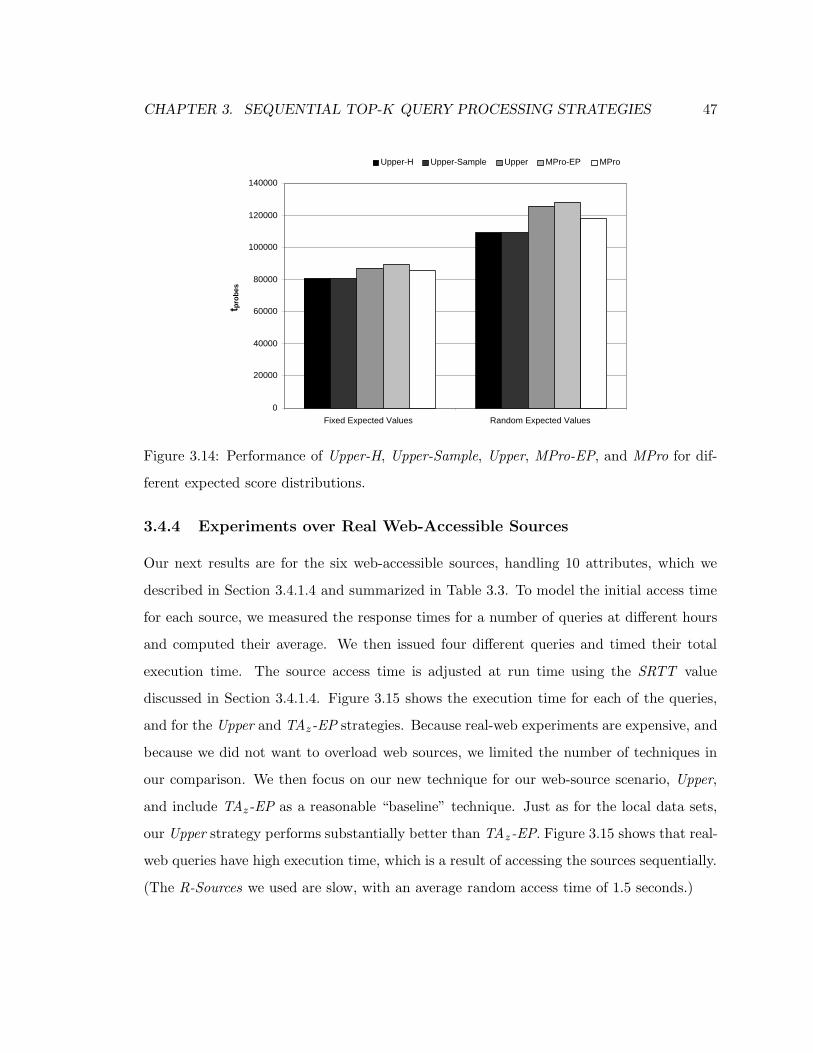
CHAPTER 3. SEQUENTIAL TOP-K QUERY PROCESSING STRATEGIES 47
0
20000
40000
60000
80000
100000
120000
140000
Fixed Expected Values Random Expected Values
t pro
bes
Upper-H Upper-Sample Upper MPro-EP MPro
Figure 3.14: Performance of Upper-H, Upper-Sample, Upper, MPro-EP, and MPro for dif-
ferent expected score distributions.
3.4.4 Experiments over Real Web-Accessible Sources
Our next results are for the six web-accessible sources, handling 10 attributes, which we
described in Section 3.4.1.4 and summarized in Table 3.3. To model the initial access time
for each source, we measured the response times for a number of queries at different hours
and computed their average. We then issued four different queries and timed their total
execution time. The source access time is adjusted at run time using the SRTT value
discussed in Section 3.4.1.4. Figure 3.15 shows the execution time for each of the queries,
and for the Upper and TAz-EP strategies. Because real-web experiments are expensive, and
because we did not want to overload web sources, we limited the number of techniques in
our comparison. We then focus on our new technique for our web-source scenario, Upper,
and include TAz-EP as a reasonable “baseline” technique. Just as for the local data sets,
our Upper strategy performs substantially better than TAz-EP. Figure 3.15 shows that real-
web queries have high execution time, which is a result of accessing the sources sequentially.
(The R-Sources we used are slow, with an average random access time of 1.5 seconds.)
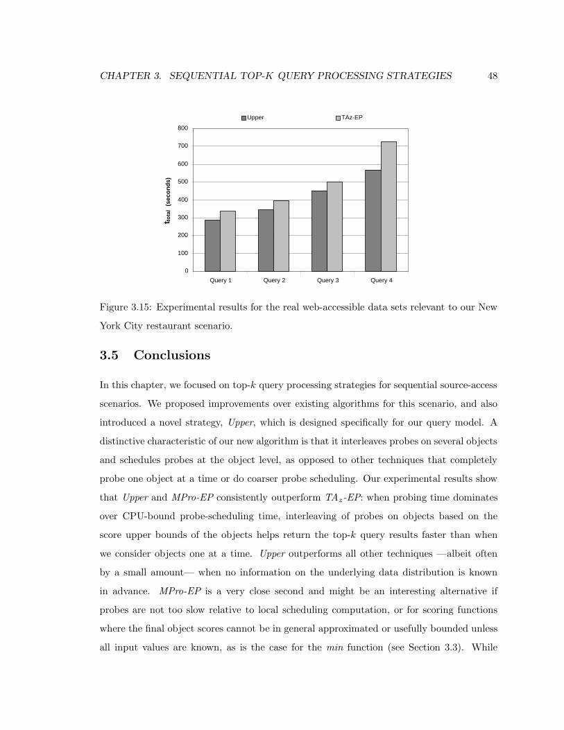
CHAPTER 3. SEQUENTIAL TOP-K QUERY PROCESSING STRATEGIES 48
0
100
200
300
400
500
600
700
800
Query 1 Query 2 Query 3 Query 4
t tota
l (s
eco
nd
s)
Upper TAz-EP
Figure 3.15: Experimental results for the real web-accessible data sets relevant to our New
York City restaurant scenario.
3.5 Conclusions
In this chapter, we focused on top-k query processing strategies for sequential source-access
scenarios. We proposed improvements over existing algorithms for this scenario, and also
introduced a novel strategy, Upper, which is designed specifically for our query model. A
distinctive characteristic of our new algorithm is that it interleaves probes on several objects
and schedules probes at the object level, as opposed to other techniques that completely
probe one object at a time or do coarser probe scheduling. Our experimental results show
that Upper and MPro-EP consistently outperform TAz-EP: when probing time dominates
over CPU-bound probe-scheduling time, interleaving of probes on objects based on the
score upper bounds of the objects helps return the top-k query results faster than when
we consider objects one at a time. Upper outperforms all other techniques —albeit often
by a small amount— when no information on the underlying data distribution is known
in advance. MPro-EP is a very close second and might be an interesting alternative if
probes are not too slow relative to local scheduling computation, or for scoring functions
where the final object scores cannot be in general approximated or usefully bounded unless
all input values are known, as is the case for the min function (see Section 3.3). While
CHAPTER 3. SEQUENTIAL TOP-K QUERY PROCESSING STRATEGIES 49
Upper’s dynamic probe scheduling is more expensive in terms of local processing time than
MPro-EP’s fixed scheduling, the saving in probing time makes Upper globally faster than
MPro-EP in total processing time (although by just a small margin) even for moderate
random access times. In addition, Upper is globally faster that TAz-EP for realistic random
access times. In conclusion, Upper results in faster query execution when probing time
dominates query execution time. When sampling is possible, a variation of Upper, Upper-
Sample, can take advantage of better expected-score estimates, which results in faster query
executions. Similarly, MPro performs well and adapts better to the data distribution than
MPro-EP does. Generally, MPro-EP (and MPro when sampling is possible) are very close
in performance to Upper, suggesting that the complexity of per-object scheduling of probes
(Table 3.1) might not be desirable. However, as we will see in Chapter 4, per-object probe
scheduling results in substantial execution-time savings in a parallel processing scenario:
per-object scheduling can adapt to intra-query source congestion on the fly, and therefore
different probing choices can be made on different objects. As a final observation, note that
all the algorithms discussed in this chapter correctly identify the top-k objects for a query
according to a given scoring function. Hence there is no need to evaluate the “correctness”
or “relevance” of the computed answers.

Chapter 4 50
Chapter 4
Parallel Top-k Query Processing
Strategies over Web-Accessible
Structured Data
In Chapter 3, we have discussed sequential top-k query processing strategies. These strat-
egies are bound to require unnecessarily long query processing times, since web accesses
usually exhibit high and variable latency. Fortunately, web sources can be probed in paral-
lel, and also each source can typically process concurrent requests. Processing top-k queries
over web sources can take full advantage of the intrinsic parallel nature of the web and issue
probes to several web sources simultaneously, possibly issuing several concurrent probes to
each individual source as well.
Example 1 (cont.): Consider our restaurant example from Chapter 2. Each source as-
sociated with the restaurant attributes, Zagat-Review, NYT-Review, and MapQuest, can be
probed in parallel. In addition, each individual source may be able to handle several con-
current accesses. For instance, MapQuest could handle, say, up to 10 concurrent probes
requesting restaurant distance information to a user address.
We use our sequential technique of Chapter 3 as the basis to define a parallel query
processing algorithm that exploits the inherently parallel nature of web sources to minimize

CHAPTER 4. PARALLEL TOP-K QUERY PROCESSING STRATEGIES 51
query response time. As we will see, making the algorithms parallel results in drastic
reductions in query processing time.
In this chapter, we make the following contributions:
• An extension of the data model from Section 3.1 to capture constraints that the
sources might impose on the number of parallel requests that they can handle at any
point in time.
• A simple parallelization of the TA algorithm [FLN01].
• An efficient parallel top-k query processing algorithm that considers source congestion
to make dynamic choices during query execution.
• A thorough, extensive experimental evaluation of the presented algorithms using real
and local data sets, and for a wide range of query parameters.
The rest of this chapter is organized as follows. First, in Section 4.1 we extend our
data model to capture the parallelism of web sources. Then, we introduce query processing
algorithms that exploit source-access parallelism to minimize query response time, while
observing source-access constraints. Specifically, in Section 4.2 we present a simple adap-
tation of the TAz algorithm to our parallel setting with source-access constraints. Then,
in Section 4.3, we present an algorithm based on Upper that considers source congestion
when making its probing choices. As we will see, this algorithm is robust and has the best
performance in our experimental evaluation of the techniques in Sections 4.4. This chapter
is based on work that has been published in [MBG04].
4.1 Parallel Data Model
On the web, sources can typically handle multiple queries in parallel. However, query pro-
cessing techniques must avoid sending large numbers of probes to sources. More specifically,
our query processing strategies must be aware of any access restrictions that the sources in
a realistic web environment might impose. Such restrictions might be due to network and
processing limitations of a source, which might bound the number of concurrent queries
CHAPTER 4. PARALLEL TOP-K QUERY PROCESSING STRATEGIES 52
that it can handle. This bound might change dynamically, and could be relaxed (e.g., at
night) when source load is lower.
Definition 4: [Source Access Constraints] Let R be a source that supports random
accesses. We refer to the maximum number of concurrent random accesses that a top-k
query processing technique can issue to R as pR(R), where pR(R) ≥ 1. In contrast, sorted
accesses to a source are sequential by nature (e.g., matches 11-20 are requested only after
matches 1-10 have been computed and returned), so we assume that we submit getNext
requests to a source sequentially when processing a query. However, random accesses can
proceed concurrently with sorted access: we will have at most one outstanding sorted access
request to a specific SR-Source S at any time, while we can have up to pR(S) outstanding
random-access requests to this same source, for a total of up to 1 + pR(S) concurrent
accesses.
Each source Di can process up to pR(Di) random accesses concurrently. Whenever
the number of outstanding probes to a source Di falls below pR(Di), a parallel processing
strategy can decide to send one more probe to Di.
4.2 A Simple Parallelization Scheme
The TA algorithm (Section 3.2.1) as described by Fagin et al. [FLN01] does not preclude
parallel executions. We adapt the TAz version of this algorithm [FLN03] to our parallel
scenario and define pTA, which probes objects in parallel in the order in which they are
retrieved from the SR-Sources, while respecting source-access constraints. Specifically, each
object retrieved via sorted access is placed in a queue of discovered objects. When a source
Di becomes available, pTA chooses which object to probe next for that source by selecting
the first object in the queue that has not yet been probed for Di. Additionally, pTA
can include the TA-Opt optimization over TAz to stop probing objects whose score cannot
exceed that of the best top-k objects already seen (Section 3.2.2). pTA then takes advantage
of all available parallel source accesses to return the top-k query answer as fast as possible.
However, it does not make choices on which probes to perform, but rather only saves probes
on “discarded” objects.
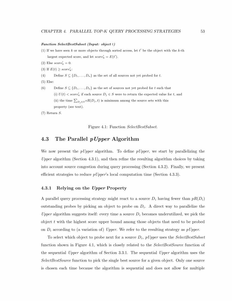
CHAPTER 4. PARALLEL TOP-K QUERY PROCESSING STRATEGIES 53
Function SelectBestSubset (Input: object t)
(1) If we have seen k or more objects through sorted access, let t′ be the object with the k-th
largest expected score, and let score′k = E(t′).
(2) Else score′k = 0.
(3) If E(t) ≥ score′k:
(4) Define S ⊆ {D1, . . . , Dn} as the set of all sources not yet probed for t.
(5) Else:
(6) Define S ⊆ {D1, . . . , Dn} as the set of sources not yet probed for t such that
(i) U(t) < score′k if each source Dj ∈ S were to return the expected value for t, and
(ii) the timeP
Dj∈S eR(Dj , t) is minimum among the source sets with this
property (see text).
(7) Return S.
Figure 4.1: Function SelectBestSubset.
4.3 The Parallel pUpper Algorithm
We now present the pUpper algorithm. To define pUpper, we start by parallelizing the
Upper algorithm (Section 4.3.1), and then refine the resulting algorithm choices by taking
into account source congestion during query processing (Section 4.3.2). Finally, we present
efficient strategies to reduce pUpper’s local computation time (Section 4.3.3).
4.3.1 Relying on the Upper Property
A parallel query processing strategy might react to a source Di having fewer than pR(Di)
outstanding probes by picking an object to probe on Di. A direct way to parallelize the
Upper algorithm suggests itself: every time a source Di becomes underutilized, we pick the
object t with the highest score upper bound among those objects that need to be probed
on Di according to (a variation of) Upper. We refer to the resulting strategy as pUpper.
To select which object to probe next for a source Di, pUpper uses the SelectBestSubset
function shown in Figure 4.1, which is closely related to the SelectBestSource function of
the sequential Upper algorithm of Section 3.3.1. The sequential Upper algorithm uses the
SelectBestSource function to pick the single best source for a given object. Only one source
is chosen each time because the algorithm is sequential and does not allow for multiple

CHAPTER 4. PARALLEL TOP-K QUERY PROCESSING STRATEGIES 54
concurrent probes to proceed simultaneously. In contrast, probes can proceed concurrently
in a parallel setting and this is reflected in the SelectBestSubset function, which generalizes
SelectBestSource and picks a minimal set of sources that need to be probed for a given object.
Intuitively, these multiple probes might proceed in parallel to speed up query execution.
When a random-access source Di becomes underutilized, we identify the object t with the
highest score upper bound such that Di ∈ SelectBestSubset(t).
4.3.2 Taking Source Congestion into Account
The SelectBestSubset function attempts to predict what probes will be performed on an
object t before the top-k answer is reached: (1) if t is expected to be one of the top-
k objects, all random accesses on sources for which t’s attribute score is missing will be
considered (Step 4); otherwise (2) only the fastest subset of probes expected to help discard
t —by decreasing t’s score upper bound below the k-th highest (expected) object score
score′k— are considered (Step 6). SelectBestSubset bases its choices on the known attribute
scores of object t at the time of the function invocation, as well as on the expected access
time eR(Dj , t) for each source Dj not yet probed for t, which is defined as the sum of two
terms:
1. The time wR(Dj , t) that object t will have to “wait in line” before being probed
for Dj : any object t′ with U(t′) > U(t) that needs to be probed for Dj will do so
before t. Then, if precede(Dj , t) denotes the number of such objects, we can define
wR(Dj , t) = bprecede(Dj ,t)
pR(Dj)c · tR(Dj). To account for the waiting time wR and the
precede(Dj , t) value for all sources accurately, objects are considered in decreasing
order of their score upper bounds.
2. The time tR(Dj) to actually perform the probe.
The time eR(Dj , t) is then equal to:
eR(Dj , t) = wR(Dj , t) + tR(Dj)
= tR(Dj) · (bprecede(Dj , t)
pR(Dj)c + 1)
CHAPTER 4. PARALLEL TOP-K QUERY PROCESSING STRATEGIES 55
Without factoring in the wR waiting time, all best subsets tend to be similar and include
only sources with high weight in the query and/or with low access time tR. Considering
the waiting time is critical to dynamically account for source congestion, and allows for
slow sources or sources with low associated query weight to be used for some objects,
thus avoiding wasting resources by not taking advantage of all available concurrent source
accesses. The fastest subset of probes expected to help discard t is chosen based on the
sum of the expected access time of its associated sources. While using their maximum value
would give a better estimation of the expected time to probe all sources in the subset, the
sum function helps to take into consideration the global source congestion that would result
from probing the subset.
As mentioned before, this SelectBestSubset function is closely related to the SelectBest-
Source function of Section 3.3.1. Both functions allow for dynamic query evaluation by
relying on current available information on object scores to make probing choices. However,
SelectBestSubset is used in a parallel setting where probes can be issued concurrently, so
there is no need to determine a total order of the source probes for each object and “subset”
probes can be issued concurrently. Therefore, the Rank metric presented in Section 3.3.1 is
not strictly needed in the SelectBestSubset function. Interestingly, in the specific scenario
where any one source is expected to be enough to discard an object t, SelectBestSubset
selects the same source for t as SelectBestSource would if we ignore the source waiting time:
in this scenario any source is expected to decrease the score upper bound of t by at least ∆
(Section 3.3.1), and SelectBestSubset picks the fastest such source. This choice is equivalent
to selecting the source with the highest Min{∆,δi}tR(Ri)
rank value, as is done by SelectBestSource.
4.3.3 Avoiding Redundant Computation
The query-processing strategy above is expensive in local computation time: it might re-
quire several calls to SelectBestSubset each time a random-access source becomes available,
and SelectBestSubset takes time that is exponential in the number of sources. To reduce
local processing time, we devise an efficient algorithm based on the following observation:
whenever SelectBestSubset is invoked to schedule probes for a source Di, information on
the best probes to perform for Di as well as for other sources is computed. Scheduling

CHAPTER 4. PARALLEL TOP-K QUERY PROCESSING STRATEGIES 56
probes for just one source at any given time results in discarding the information on valu-
able probes to the other sources, which results in redundant computation when these other
sources become underutilized and can then receive further probes.
Time t Time t +1
D 1
D 3
D 2
o 1
o 1 finishes
o 2 o 2
o 1
o 3 flush and regenerate all
source queues
o 3
o 2 o 4
Queue(D 1 )
Queue(D 2 )
Queue(D 3 )
o 5
o 3 o 1
o 5 o 4
Queue(D 1 )
Queue(D 2 )
Queue(D 3 )
Figure 4.2: An execution step of pUpper.
With the above observations in mind, our parallel top-k processing algorithm, pUpper,
precomputes sets of objects to probe for each source. When a source becomes available,
pUpper checks whether an object to probe for that source has already been chosen. If not,
pUpper recomputes objects to probe for all sources, as shown in Figure 4.2. This way,
earlier choices of probes on any source might be revised in light of new information on
object scores: objects that appeared “promising” earlier (and hence that might have been
scheduled for further probing) might now be judged less promising than other objects after
some probes complete. By choosing several objects to probe for every source in a single
computation, pUpper drastically reduces local processing time.
The pUpper algorithm (Figure 4.3) associates a queue with each source for random access
scheduling. The queues are regularly updated by calls to the function GenerateQueues
(Figure 4.4). During top-k query processing, if a source Di is available, pUpper checks the
associated random-access queue Queue(Di). If Queue(Di) is empty, then all random access
queues are regenerated (Steps 7-8 in Figure 4.3). If Queue(Di) is not empty, then simply a
probe to Di on the first object in Queue(Di) is sent (Steps 9-11). To avoid repeated calls to
GenerateQueues when a random access queue is continuously empty (which can happen, for

CHAPTER 4. PARALLEL TOP-K QUERY PROCESSING STRATEGIES 57
Algorithm pUpper (Input: top-k query q)
(01) Repeat
(02) For each SR-Source Di (1 ≤ i ≤ nsr):
(03) If no sorted access is being performed on Di and more objects are available from Di
for q :
(04) Call pGetNext(Di , q) asynchronously.
(05) For each source Di (1 ≤ i ≤ n):
(06) While fewer that pR(Di) random accesses are being performed on Di:
(07) If Queue(Di) = ∅:
(08) GenerateQueues().
(09) Else:
(10) t = Dequeue(Di).
(11) Call pGetScore(Di , q, t) asynchronously.
(12) Until we have identified k top objects
(13) Return the top-k objects along with their scores.
Figure 4.3: Algorithm pUpper.
example, if all known objects have already been probed for its associated source), a queue
left empty from a previous execution does not trigger a new call to GenerateQueues.
As sorted accesses are sequential in nature (Definition 4, Section 4.1), pUpper attempts
to always have exactly one outstanding sorted-access request per SR-Source Di (Steps 2-4).
As soon as a sorted access to Di completes, a new one is sent until all needed objects are
retrieved from Di.
Source accesses are performed by calling pGetNext and pGetScore, which are asyn-
chronous versions of the getNext and getScore source interfaces (Definition 1); these
asynchronous calls, similar to the asynchronous iteration described in WSQ/DSQ [GW00],
allow the query processing algorithm to continue without waiting for the source accesses
to complete. pGetNext and pGetScore send the corresponding probes to the sources, wait
for their results to return, and update the appropriate data structures with the new infor-
mation. Of course, pUpper keeps track of outstanding probes so as not to issue duplicate
probes. The top-k query processing terminates when the top-k objects are identified, which
happens when no object can have a final score greater than that of any of the current top-k

CHAPTER 4. PARALLEL TOP-K QUERY PROCESSING STRATEGIES 58
Function GenerateQueues()
(1) Let Considered be the set of “alive” objects (i.e., objects whose score upper bound is greater
than the k-th largest score lower bound).
(2) For each source Di (1 ≤ i ≤ n):
(3) Empty Queue(Di).
(4) While Considered 6= ∅ and ∃i ∈ {1, ..., n} : |Queue(Di)| < L:
(5) Extract tH from Considered such that: U(tH) = maxt∈Considered U(t).
(6) S = SelectBestSubset(tH).
(7) For each source Dj ∈ S:
(8) If |Queue(Dj)| < L: Enqueue(Dj , tH).
Figure 4.4: Function GenerateQueues.
objects.
To allow for dynamic queue updates at regular intervals, and to ensure that queues are
generated using recent information, we define a parameter L that indicates the length of the
random-access queues generated by the GenerateQueues function. A call to GenerateQueues
to populate a source’s random-access queue provides up-to-date information on current
best objects to probe for all sources, therefore GenerateQueues regenerates all random-
access queues. An object t is only inserted into the queues of the sources returned by the
SelectBestSubset(t) function from Figure 4.1 (Steps 6-8 in Figure 4.4). Additionally, objects
are considered in the order of their score upper bound (Step 5), considering only “alive”
objects, i.e., objects that have not been discarded (Step 1).
pUpper precomputes a list of objects to access per source, based on expected score values.
Of course, the best subset for an object might vary during processing, and pUpper might
perform “useless” probes. Parameter L regulates the tradeoff between queue “freshness”
and local processing time, since L determines how frequently the random access queues are
updated and how reactive pUpper is to new information.
4.4 Experimental Results
We performed an extensive experimental evaluation of pUpper. In this section, we first
discuss our implementation choices and evaluation settings (Section 4.4.1), then report
CHAPTER 4. PARALLEL TOP-K QUERY PROCESSING STRATEGIES 59
results over local data sets (Section 4.4.2), compare pUpper with a state-of-the-art parallel
top-k query processing strategy (Section 4.4.3), and present results over real web sources
(Section 4.4.4).
4.4.1 Implementation
In this section, we describe the query processing techniques that participated in our exper-
imental evaluation (Section 4.4.1.1), and discuss the evaluation metrics we use to evaluate
our parallel strategies (Section 4.4.1.2). We implemented the parallel top-k query processing
strategies in C++, using POSIX threads and multiple Python subinterpreters to support
concurrency. Our implementation takes advantage of the same data structures from the se-
quential case (Section 3.4.1.2). Finally, we evaluated our parallel techniques over the same
data sets as the sequential techniques (Sections 3.4.1.3 and 3.4.1.4).
4.4.1.1 Techniques
We compare the performance of pUpper (Section 4.3) with that of pTA (Section 4.2). pUpper
is a technique in which source probes are scheduled at a fine object-level granularity, and
where reevaluation of probing choices can lead objects to be probed in different orders for
different sources. In contrast, pTA is a technique in which objects are probed in the same
order for all sources. In addition, we compare these two techniques with pUpper-NoSubsets,
a simplification of pUpper that does not rely on the SelectBestSubset function to make its
probing choices. Rather, when a source Di becomes available, pUpper-NoSubsets selects
the object with the highest score upper bound among the objects not yet probed on Di.
pUpper-NoSubsets is then similar to pTA, but with the difference that objects are considered
in score-upper-bound order rather than in the order in which they are discovered.
By comparing pUpper-NoSubsets and pTA, our experiments help identify the saving in
probing time that is derived from prioritizing objects on their partial scores. By comparing
pUpper-NoSubsets and pUpper, our experiments help understand the impact of dynamically
selecting probes in a way that accounts for source congestion and known source-score in-
formation. These three techniques all react to a source Di being available to pick a probe
to issue next. In Section 4.4.2.2, we compare these techniques with Probe-Parallel MPro,

CHAPTER 4. PARALLEL TOP-K QUERY PROCESSING STRATEGIES 60
a parallelization of MPro presented in [CH02]. Unlike the other techniques, Probe-Parallel
MPro does not consider source availability to issue its probes (recall that MPro was origi-
nally designed for a different setting, namely the execution of expensive predicates for top-k
queries, not for our web-source scenario) but is based on the concept of “necessary probes,”
and thus only issues probes that are known to be needed to compute the top-k answer.
To deploy the pUpper algorithm, we first need to experimentally establish a good value
for the L parameter, which determines how frequently the random-access queues are up-
dated (Section 4.3). To tune this parameter, we ran experiments over a number of local
sources for different settings of |Objects|, pR, and k. As expected, smaller values of L result
in higher local processing time. Interestingly, while the query response time increases with
L, very small values of L (i.e., L < 30) yield larger tprobes values than moderate values of
L (i.e., 50 ≤ L ≤ 200) do: when L is small, pUpper tends to “rush” into performing probes
that would have otherwise been discarded later. We observed that L = 100 is a robust
choice for moderate to large database sizes and for the query parameters that we tried.
Thus, we set L to 100 for the local data experiments.
4.4.1.2 Parallelism
In addition to reporting on the metrics described in Section 3.4.1.5, we need to quantify the
extent to which the parallel techniques exploit the available source-access parallelism. Con-
sider Upper, the sequential algorithm that performed the best for our web-source scenario
(with relatively expensive probes and no information on the underlying data distribution
known in advance) according to the experimental evaluation in Section 3.4. Ideally, par-
allel algorithms would keep sources “humming” by accessing them in parallel as much as
possible. At any point in time, up to nsr +∑n
i=1 pR(Di) concurrent source accesses can
be in progress. Hence, if tUpper is the time that Upper spends accessing remote sources se-
quentially, then tUpper/(nsr +∑n
i=1 pR(Di)) is a (loose) lower bound on the parallel tprobes
time for the parallel algorithms, assuming that parallel algorithms perform at least as many
source accesses as Upper. To observe what fraction of this potential parallel speedup the
parallel algorithms achieve, we report:
Parallel Efficiency =tUpper/(nsr +
∑ni=1 pR(Di))
tprobes
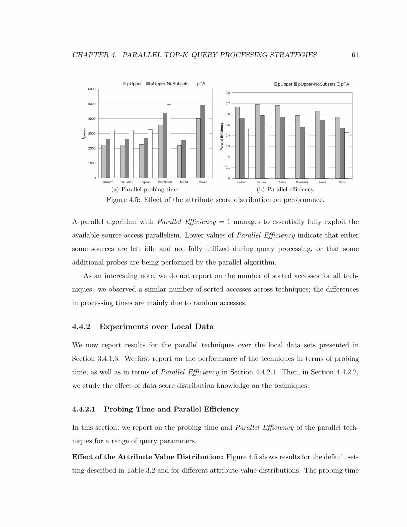
CHAPTER 4. PARALLEL TOP-K QUERY PROCESSING STRATEGIES 61
0
1000
2000
3000
4000
5000
6000
Uniform Gaussian Zipfian Correlated Mixed Cover
t pro
bes
pUpper pUpper-NoSubsets pTA
(a) Parallel probing time.
0
0.1
0.2
0.3
0.4
0.5
0.6
0.7
0.8
Uniform Gaussian Zipfian Correlated Mixed Cover
Par
alle
l Eff
icie
ncy
pUpper pUpper-NoSubsets pTA
(b) Parallel efficiency.
Figure 4.5: Effect of the attribute score distribution on performance.
A parallel algorithm with Parallel Efficiency = 1 manages to essentially fully exploit the
available source-access parallelism. Lower values of Parallel Efficiency indicate that either
some sources are left idle and not fully utilized during query processing, or that some
additional probes are being performed by the parallel algorithm.
As an interesting note, we do not report on the number of sorted accesses for all tech-
niques: we observed a similar number of sorted accesses across techniques; the differences
in processing times are mainly due to random accesses.
4.4.2 Experiments over Local Data
We now report results for the parallel techniques over the local data sets presented in
Section 3.4.1.3. We first report on the performance of the techniques in terms of probing
time, as well as in terms of Parallel Efficiency in Section 4.4.2.1. Then, in Section 4.4.2.2,
we study the effect of data score distribution knowledge on the techniques.
4.4.2.1 Probing Time and Parallel Efficiency
In this section, we report on the probing time and Parallel Efficiency of the parallel tech-
niques for a range of query parameters.
Effect of the Attribute Value Distribution: Figure 4.5 shows results for the default set-
ting described in Table 3.2 and for different attribute-value distributions. The probing time

CHAPTER 4. PARALLEL TOP-K QUERY PROCESSING STRATEGIES 62
0
1000
2000
3000
4000
5000
6000
7000
0 100 200 300 400 500
k
t pro
bes
pUpper pUpper-NoSubsets pTA
(a) Parallel probing time.
0
0.1
0.2
0.3
0.4
0.5
0.6
0.7
0.8
0 100 200 300 400 500
k
Par
alle
l Eff
icie
ncy
pUpper pUpper-NoSubsets pTA
(b) Parallel efficiency.
Figure 4.6: Effect of the number of objects requested k on performance.
tprobes of pUpper, pUpper-NoSubsets, and pTA is reported in Figure 4.5(a). pUpper consis-
tently outperforms both pTA and pUpper-NoSubsets. The dynamic per-object scheduling of
pUpper, which takes into account source congestion, allows for substantial savings over the
simpler pUpper-NoSubsets technique. Figure 4.5(b) shows that pTA’s Parallel Efficiency
varies slightly among all configurations, with values around 0.45. In contrast, pUpper’s
Parallel Efficiency ranges from 0.57 (Cover data set) to 0.69 (Gaussian data set), with
values of 0.59 for the Correlated data sets, 0.63 for the Mixed data set, 0.67 for the Uniform
data set, and 0.68 for the Zipfian data set.
Effect of the Number of Objects Requested k: Figure 4.6 shows results for the
default setting, with tprobes and Parallel Efficiency reported as a function of k. As k
increases, the parallel time needed by pTA, pUpper-NoSubsets, and pUpper increases since
all three techniques need to retrieve and process more objects (Figure 4.6(a)). The pUpper
strategy consistently outperforms pTA, with the performance of pUpper-NoSubsets between
that of pTA and pUpper. The Parallel Efficiency of pUpper, pUpper-NoSubsets, and pTA is
almost constant across different values of k (Figure 4.6(b)), with Upper attaining Parallel
Efficiency values of around 0.68, which roughly means it is only one third slower than an
ideal parallelization of Upper.
Effect of the Cardinality of the Objects Set: Figure 4.7 shows the impact of |Objects|,
the number of objects available in the sources. As the number of objects increases, the

CHAPTER 4. PARALLEL TOP-K QUERY PROCESSING STRATEGIES 63
0
5000
10000
15000
20000
25000
30000
35000
40000
0 50000 100000 150000 200000
|Objects|
t pro
bes
pUpper pUpper-NoSubsets pTA
(a) Parallel probing time.
0
0.1
0.2
0.3
0.4
0.5
0.6
0.7
0.8
0 50000 100000 150000 200000
|Objects|
Par
alle
l Eff
icie
ncy
pUpper pUpper-NoSubsets pTA
(b) Parallel efficiency.
Figure 4.7: Effect of the number of source objects |Objects| on performance.
0
2000
4000
6000
8000
10000
12000
0 5 10 15 20 25
pR(D i )
t pro
bes
pUpper pUpper-NoSubsets pTA
(a) Parallel probing time.
0
0.2
0.4
0.6
0.8
1
1.2
0 5 10 15 20 25
pR(D i )
Par
alle
l Eff
icie
ncy
pUpper pUpper-NoSubsets pTA
(b) Parallel efficiency.
Figure 4.8: Effect of the number of parallel accesses per source pR(Di) on performance.
parallel time taken by all three algorithms increases since more objects need to be processed.
The parallel time of pTA, pUpper-NoSubsets, and pUpper increases approximatively linearly
with |Objects| (Figure 4.7(a)). The Parallel Efficiency of all three algorithms decreases
slightly with the number of objects.
Effect of the Number of Parallel Accesses to each Source pR(Di): Figure 4.8
reports performance results as a function of the total number of concurrent random accesses
per source. As expected, the parallel query time decreases when the number of parallel
accesses increases (Figure 4.8(a)). However, pTA, pUpper-NoSubsets, and pUpper have
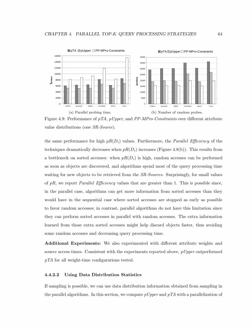
CHAPTER 4. PARALLEL TOP-K QUERY PROCESSING STRATEGIES 64
0
2000
4000
6000
8000
10000
12000
14000
16000
Uniform Gaussian Zipfian Correlated Mixed Cover
t pro
bes
pTA pUpper PP-MPro-Constraints
(a) Parallel probing time.
0
5000
10000
15000
20000
25000
30000
35000
40000
Uniform Gaussian Zipfian Correlated Mixed Cover
|pro
bes
|
pTA pUpper PP-MPro-Constraints
(b) Number of random probes.
Figure 4.9: Performance of pTA, pUpper, and PP-MPro-Constraints over different attribute
value distributions (one SR-Source).
the same performance for high pR(Di) values. Furthermore, the Parallel Efficiency of the
techniques dramatically decreases when pR(Di) increases (Figure 4.8(b)). This results from
a bottleneck on sorted accesses: when pR(Di) is high, random accesses can be performed
as soon as objects are discovered, and algorithms spend most of the query processing time
waiting for new objects to be retrieved from the SR-Sources. Surprisingly, for small values
of pR, we report Parallel Efficiency values that are greater than 1. This is possible since,
in the parallel case, algorithms can get more information from sorted accesses than they
would have in the sequential case where sorted accesses are stopped as early as possible
to favor random accesses; in contrast, parallel algorithms do not have this limitation since
they can perform sorted accesses in parallel with random accesses. The extra information
learned from those extra sorted accesses might help discard objects faster, thus avoiding
some random accesses and decreasing query processing time.
Additional Experiments: We also experimented with different attribute weights and
source access times. Consistent with the experiments reported above, pUpper outperformed
pTA for all weight-time configurations tested.
4.4.2.2 Using Data Distribution Statistics
If sampling is possible, we can use data distribution information obtained from sampling in
the parallel algorithms. In this section, we compare pUpper and pTA with a parallelization of
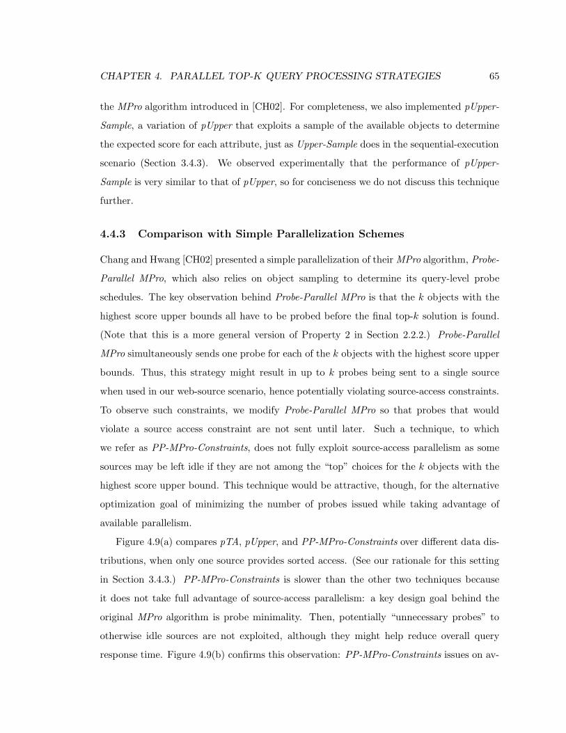
CHAPTER 4. PARALLEL TOP-K QUERY PROCESSING STRATEGIES 65
the MPro algorithm introduced in [CH02]. For completeness, we also implemented pUpper-
Sample, a variation of pUpper that exploits a sample of the available objects to determine
the expected score for each attribute, just as Upper-Sample does in the sequential-execution
scenario (Section 3.4.3). We observed experimentally that the performance of pUpper-
Sample is very similar to that of pUpper, so for conciseness we do not discuss this technique
further.
4.4.3 Comparison with Simple Parallelization Schemes
Chang and Hwang [CH02] presented a simple parallelization of their MPro algorithm, Probe-
Parallel MPro, which also relies on object sampling to determine its query-level probe
schedules. The key observation behind Probe-Parallel MPro is that the k objects with the
highest score upper bounds all have to be probed before the final top-k solution is found.
(Note that this is a more general version of Property 2 in Section 2.2.2.) Probe-Parallel
MPro simultaneously sends one probe for each of the k objects with the highest score upper
bounds. Thus, this strategy might result in up to k probes being sent to a single source
when used in our web-source scenario, hence potentially violating source-access constraints.
To observe such constraints, we modify Probe-Parallel MPro so that probes that would
violate a source access constraint are not sent until later. Such a technique, to which
we refer as PP-MPro-Constraints, does not fully exploit source-access parallelism as some
sources may be left idle if they are not among the “top” choices for the k objects with the
highest score upper bound. This technique would be attractive, though, for the alternative
optimization goal of minimizing the number of probes issued while taking advantage of
available parallelism.
Figure 4.9(a) compares pTA, pUpper, and PP-MPro-Constraints over different data dis-
tributions, when only one source provides sorted access. (See our rationale for this setting
in Section 3.4.3.) PP-MPro-Constraints is slower than the other two techniques because
it does not take full advantage of source-access parallelism: a key design goal behind the
original MPro algorithm is probe minimality. Then, potentially “unnecessary probes” to
otherwise idle sources are not exploited, although they might help reduce overall query
response time. Figure 4.9(b) confirms this observation: PP-MPro-Constraints issues on av-
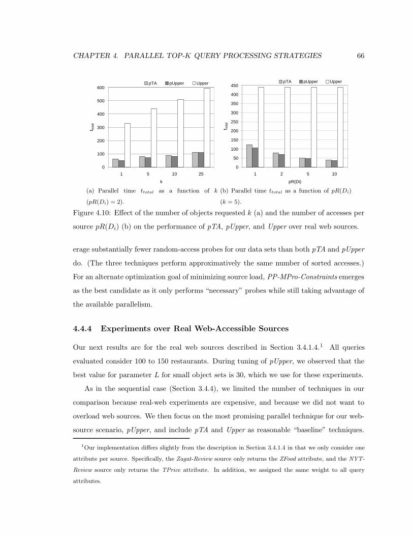
CHAPTER 4. PARALLEL TOP-K QUERY PROCESSING STRATEGIES 66
0
100
200
300
400
500
600
1 5 10 25
k
t tota
l
pTA pUpper Upper
(a) Parallel time ttotal as a function of k
(pR(Di) = 2).
0
50
100
150
200
250
300
350
400
450
1 2 5 10
pR(Di)
t tota
l
pTA pUpper Upper
(b) Parallel time ttotal as a function of pR(Di)
(k = 5).
Figure 4.10: Effect of the number of objects requested k (a) and the number of accesses per
source pR(Di) (b) on the performance of pTA, pUpper, and Upper over real web sources.
erage substantially fewer random-access probes for our data sets than both pTA and pUpper
do. (The three techniques perform approximatively the same number of sorted accesses.)
For an alternate optimization goal of minimizing source load, PP-MPro-Constraints emerges
as the best candidate as it only performs “necessary” probes while still taking advantage of
the available parallelism.
4.4.4 Experiments over Real Web-Accessible Sources
Our next results are for the real web sources described in Section 3.4.1.4.1 All queries
evaluated consider 100 to 150 restaurants. During tuning of pUpper, we observed that the
best value for parameter L for small object sets is 30, which we use for these experiments.
As in the sequential case (Section 3.4.4), we limited the number of techniques in our
comparison because real-web experiments are expensive, and because we did not want to
overload web sources. We then focus on the most promising parallel technique for our web-
source scenario, pUpper, and include pTA and Upper as reasonable “baseline” techniques.
1Our implementation differs slightly from the description in Section 3.4.1.4 in that we only consider one
attribute per source. Specifically, the Zagat-Review source only returns the ZFood attribute, and the NYT-
Review source only returns the TPrice attribute. In addition, we assigned the same weight to all query
attributes.

CHAPTER 4. PARALLEL TOP-K QUERY PROCESSING STRATEGIES 67
Figure 4.10(a) shows the actual total execution time (in seconds) of pTA, pUpper, and the
sequential algorithm Upper for different values of the number of objects requested k. Up to
two concurrent accesses can be sent to each R-Source Di (i.e., pR(Di) = 2). Figure 4.10(b)
shows the total execution time of the same three algorithms for a top-5 query when we vary
the number of parallel random accesses available for each source pR(Di). (Note that pR
does not apply to Upper, which is a sequential algorithm.) When the number of parallel
random accesses to the sources increases, the difference in query execution time between
pTA and pUpper becomes small. This is consistent with what we observed on the local data
sets (see Section 4.4.2, Figure 4.8), and is due to sorted accesses becoming a bottleneck and
slowing down query execution. We also performed experiments varying the relative weights
of the different sources. In general, our results are consistent with those for local sources,
and pUpper and pTA significantly reduce query processing time compared to Upper. We
observed that a query needs 20 seconds on average to perform all needed sorted accesses,
so our techniques cannot return an answer in less than 20 seconds. For all methods, an
initialization time that is linear in the number of parallel accesses is needed to create the
Python subinterpreters (e.g., this time was equal to 12 seconds for pR(Di) = 5). We do
not include this uniform initialization time in Figure 4.10. Interestingly, we noticed that
sometimes random access time increases when the number of parallel accesses to that source
increases, which might be caused by sources slowing down accesses from a single application
after exceeding some concurrency level, or by sources not being able to handle the increased
parallel load. When the maximum number of accesses per source is 10, pUpper returns the
top-k query results in 35 seconds. For a realistic setting of five random accesses per source,
pUpper is the fastest technique and returns query answers in less than one minute. In
contrast, the sequential algorithm Upper needs seven minutes to return the same answer.
In a web environment, where users are unwilling to wait long for an answer and delays of
more than a minute are generally unacceptable, pUpper manages to answer top-k queries
in drastically less time than its sequential counterparts.
CHAPTER 4. PARALLEL TOP-K QUERY PROCESSING STRATEGIES 68
4.5 Conclusions
Independent of the choice of probe-scheduling algorithm, a crucial problem with sequential
top-k query processing techniques is that they do not take advantage of the inherently
parallel access nature of web sources, and spend most of their query execution time waiting
for web accesses to return. To alleviate this problem, we used the sequential Upper algorithm
(Chapter 3) as the basis to define an efficient parallel top-k query processing technique,
pUpper, which minimizes query response time while taking source-access constraints that
arise in real-web settings into account. Furthermore, just like Upper, pUpper schedules
probes at a per-object level, and can thus consider intra-query source congestion when
scheduling probes. We evaluated pTA, a simple parallelization of TA [FLN01] and pUpper
on both local and real-web sources. Both algorithms exploit the available source parallelism,
while respecting source-access constraints. pUpper is faster than pTA: pUpper carefully
selects the probes for each object, continuously reevaluating its choices. Specifically, pUpper
considers probing time and source congestion to make its probing choices at a per-object
level, which results in faster query processing and better use of the available parallelism. In
general, our results show that parallel probing significantly decreases query processing time.
For example, when the number of available concurrent accesses over six real web sources is
set to five per source, pUpper performs 9 times faster than its sequential counterpart Upper,
returning the top-k query results —on average— in under one minute. In addition, our
techniques are faster than our adaptation of Probe-Parallel MPro as they take advantage
of all the available source-access parallelism.

Chapter 5 69
Chapter 5
Top-k Query Processing Strategies
over Semi-structured Data
The need for exchanging information from one application to another, either for busi-
ness purposes or for the integration of systems that were designed separately, is increasing
steadily. Unfortunately, structured data models such as the relational model are too strict,
as they require the data to conform to a rigid and uniform structure. The semi-structured
data model [PGMW95, AQM+97] has been proposed as a more flexible alternative to rep-
resent data that might not be fully uniform and homogeneous. The eXtended Markup Lan-
guage (XML) [XML] has emerged as the format of choice for exchanging semi-structured
data from different sources that may not share the same schema. An increasing number of
large XML repositories are used to store such heterogeneous XML data (e.g., the Library
of Congress1, INEX2), raising the need for efficient query processing over heterogeneous
XML data. In this chapter, we focus on an XML integration scenario. In this scenario, as
in the previous web source scenario, exact query matches on the object contents are too
rigid; furthermore, relevant data conforming to a schema that differs only slightly from the
query schema may be missed. Therefore, top-k query processing is a natural choice for
XML integration scenarios, allowing for flexible query answers, to return the k objects that
1http://lcweb.loc.gov/crsinfo/xml/
2http://www.is.informatik.uni-duisburg.de/projects/inex03/

CHAPTER 5. TOP-K QUERIES OVER SEMI-STRUCTURED DATA 70
are closest to the query in terms of structure and content.
��� ��� ���� ��� �
����� ����������� �������
������ !� ��" � �!#$�������
��%�� ��� ������ � � � �& ����#'�
& ����#
��� ��� ����( ��� �
�)�*� ����������� �������
���+�� � ��" � �!#$�������
��%,� ��� ������ � � � �& ���!#-�
& �*��#
� �!. �
/10 2 /1030 2
Figure 5.1: XML queries on the heterogeneous book collection.
Example 2 (cont.): Consider our heterogeneous data collection example from Chapter 2
and illustrated in Figure 2.1. Books in this heterogeneous XML collection might originate
in a variety of XML data sources, each exhibiting a different XML schema. A query for
the top-3 “book” elements with children nodes (attributes) “title”=“Great Expectations”,
“author”=“Dickens”, and “edition”=“paperback”, as illustrated in Figure 5.1(i), does not
result in any exact match from the example XML collection. However, intuitively all three
data fragments (a), (b), and (c) are reasonable answers to such a query, and should be
returned as approximate query answers. Similarly, the slightly more structured query illus-
trated in Figure 5.1(ii) does not result in any exact match from the example XML collection,
but all three fragments (a), (b), and (c) are also reasonable approximate answers to such a
query.
To include approximate query matches, we rank candidate XML data fragments based
on their “similarity” to the queries, in terms of both content and structure. A data fragment
that has a query structure close to that of the query is returned as an approximate answer
to the query, and is assigned a score that depends on the closeness between the query and
data fragment structures. For instance, data fragment (a) in Figure 2.1 is closer to query
(ii) in Figure 5.1 than data fragment (b), as all of the query nodes appear in fragment (a),
whereas the edition node is missing from fragment (b).

CHAPTER 5. TOP-K QUERIES OVER SEMI-STRUCTURED DATA 71
Processing top-k queries efficiently over XML queries is challenging, as the number
of candidate answers increases dramatically with the query size. The query relaxation
framework defined in [AYLP04] provides a mechanism to represent the variations in the
structure of data fragments with respect to a query. Specifically, in this chapter we use
XML query relaxations to represent changes in the query structure and content, as proposed
in [AYCS02, DR01, Sch02] (see Section 5.1.2). By pruning irrelevant data fragments as early
as possible using Properties 1 and 2 from Section 2.2, we design adaptive algorithms that
minimize the number of candidate answers considered during query evaluation.
In this chapter, we make the following contributions:
• A data model that captures XML query approximation, and a novel mechanism for
scoring approximate answers to XML queries.
• A novel architecture incorporating a family of adaptive top-k query algorithms that
take into account the number of intermediate partially evaluated objects to make
query routing decisions.
• A thorough, extensive experimental evaluation of the new algorithms for a wide range
of architecture options and query parameters.
The rest of this chapter is organized as follows. First, we review some background on
XML data and XML query relaxation in Section 5.1. Then, in Section 5.2, we present
our data model. In Section 5.3, we describe the Whirlpool architecture and algorithms. In
Section 5.4, we report on an extensive experimental evaluation of Whirlpool. Finally, we
conclude this chapter in Section 5.5. This chapter is based on work that has been published
in [MAYKS05].
5.1 Background
In this section, we give a brief overview of XML and semi-structured data (Section 5.1.1),
and review the XML query relaxations on which we rely to provide approximate answers
to queries over XML data (Section 5.1.2).
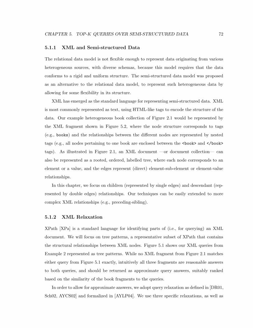
CHAPTER 5. TOP-K QUERIES OVER SEMI-STRUCTURED DATA 72
5.1.1 XML and Semi-structured Data
The relational data model is not flexible enough to represent data originating from various
heterogeneous sources, with diverse schemas, because this model requires that the data
conforms to a rigid and uniform structure. The semi-structured data model was proposed
as an alternative to the relational data model, to represent such heterogeneous data by
allowing for some flexibility in its structure.
XML has emerged as the standard language for representing semi-structured data. XML
is most commonly represented as text, using HTML-like tags to encode the structure of the
data. Our example heterogeneous book collection of Figure 2.1 would be represented by
the XML fragment shown in Figure 5.2, where the node structure corresponds to tags
(e.g., books) and the relationships between the different nodes are represented by nested
tags (e.g., all nodes pertaining to one book are enclosed between the <book> and </book>
tags). As illustrated in Figure 2.1, an XML document —or document collection— can
also be represented as a rooted, ordered, labelled tree, where each node corresponds to an
element or a value, and the edges represent (direct) element-sub-element or element-value
relationships.
In this chapter, we focus on children (represented by single edges) and descendant (rep-
resented by double edges) relationships. Our techniques can be easily extended to more
complex XML relationships (e.g., preceding-sibling).
5.1.2 XML Relaxation
XPath [XPa] is a standard language for identifying parts of (i.e., for querying) an XML
document. We will focus on tree patterns, a representative subset of XPath that contains
the structural relationships between XML nodes. Figure 5.1 shows our XML queries from
Example 2 represented as tree patterns. While no XML fragment from Figure 2.1 matches
either query from Figure 5.1 exactly, intuitively all three fragments are reasonable answers
to both queries, and should be returned as approximate query answers, suitably ranked
based on the similarity of the book fragments to the queries.
In order to allow for approximate answers, we adopt query relaxation as defined in [DR01,
Sch02, AYCS02] and formalized in [AYLP04]. We use three specific relaxations, as well as

CHAPTER 5. TOP-K QUERIES OVER SEMI-STRUCTURED DATA 73
...
<book>
<info>
<author> Dickens </author>
<title> Great Expectations </title>
</info>
<edition> paperback </edition>
</book>
<book>
<info>
<author> Dickens </author>
<title> Great Expectations </title>
</info>
</book>
<book>
<info>
<edition> paperback </edition>
<title> Great Expectations </title>
</info>
<author> Dickens </author>
</book>
...
Figure 5.2: A heterogeneous XML book collection.
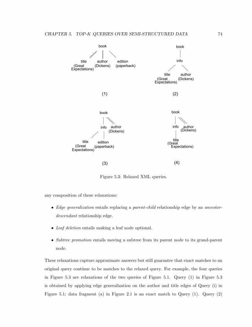
CHAPTER 5. TOP-K QUERIES OVER SEMI-STRUCTURED DATA 74
�����
��������� ��������
������
��� �����
�������
�������� ��
����
�����
��������� ��������
������
��� �����
����
����
��� ���
�����������
��� ��������
������
��� �����
��������������� ��
����
����
���
�������������� ��������
��������� �����
����
����
���
Figure 5.3: Relaxed XML queries.
any composition of these relaxations:
• Edge generalization entails replacing a parent-child relationship edge by an ancestor-
descendant relationship edge.
• Leaf deletion entails making a leaf node optional.
• Subtree promotion entails moving a subtree from its parent node to its grand-parent
node.
These relaxations capture approximate answers but still guarantee that exact matches to an
original query continue to be matches to the relaxed query. For example, the four queries
in Figure 5.3 are relaxations of the two queries of Figure 5.1. Query (1) in Figure 5.3
is obtained by applying edge generalization on the author and title edges of Query (i) in
Figure 5.1; data fragment (a) in Figure 2.1 is an exact match to Query (1). Query (2)

CHAPTER 5. TOP-K QUERIES OVER SEMI-STRUCTURED DATA 75
in Figure 5.3 is obtained by applying leaf deletion on the edition subtree of Query (ii) in
Figure 5.1; data fragment (b) in Figure 2.1 is an exact match to Query (2). Query (3)
in Figure 5.3 is obtained by applying subtree promotion on the author subtree of Query
(ii) in Figure 5.1; data fragment (c) in Figure 2.1 is an exact match to Query (3). Query
(4) in Figure 5.3 is obtained by applying leaf deletion on the edition subtree, and subtree
promotion on the author subtree of Query (ii) in Figure 5.1; data fragment (a), (b), and
(c) in Figure 2.1 are exact matches to Query (4).
As illustrated by the above example, applying relaxations to a query results in more
data collection fragments matching the (relaxed) query. By combining several relaxations
on a query we are able to match more fragments from the XML data collection. Exact
matches to a relaxed version of a query are approximate answers to the original (unrelaxed)
query. To distinguish between different answers, we need to compute scores for each match
that account for the relaxations applied to the query. We focus on this issue in Section 5.2.
5.2 XML Data Model
In our XML integration scenario, an answer to a top-k query is an XML data fragment that
approximately matches the query. Specifically, an answer to the query is a node —or XML
object— that corresponds to the query’s root node (e.g., “book” in Example 2). In this
section, we refine the data and query model of Chapter 2 and instantiate it to our XML
scenario. In this scenario, the object query attributes (or predicates) are accessed through
indexes to the different XML nodes present in the document collection. For instance, to
retrieve the “title” attribute of a book object in Example 2, we would have to perform a
join between the book object and all “title” nodes in the collection, and keep only those
nodes that are contained in the subtree rooted at the object’s book node. In this setting,
an operation aimed at retrieving an attribute for one object may yield several answers, akin
to joins in RDBMS.
Definition 5: [XML Joins] Consider an attribute Ai and a top-k query q. For a given
object t, we can obtain a set of values a1, ..., an for Ai that correspond to the XML nodes
that match attribute Ai and are contained in the data tree rooted at object t’s query root
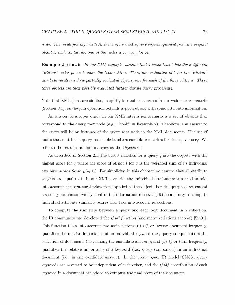
CHAPTER 5. TOP-K QUERIES OVER SEMI-STRUCTURED DATA 76
node. The result joining t with Ai is therefore a set of new objects spawned from the original
object t, each containing one of the nodes a1, . . . , an for Ai.
Example 2 (cont.): In our XML example, assume that a given book b has three different
“edition” nodes present under the book subtree. Then, the evaluation of b for the “edition”
attribute results in three partially evaluated objects, one for each of the three editions. These
three objects are then possibly evaluated further during query processing.
Note that XML joins are similar, in spirit, to random accesses in our web source scenario
(Section 3.1), as the join operation extends a given object with some attribute information.
An answer to a top-k query in our XML integration scenario is a set of objects that
correspond to the query root node (e.g., “book” in Example 2). Therefore, any answer to
the query will be an instance of the query root node in the XML documents. The set of
nodes that match the query root node label are candidate matches for the top-k query. We
refer to the set of candidate matches as the Objects set.
As described in Section 2.1, the best k matches for a query q are the objects with the
highest score for q where the score of object t for q is the weighted sum of t’s individual
attribute scores ScoreAi(qi, ti). For simplicity, in this chapter we assume that all attribute
weights are equal to 1. In our XML scenario, the individual attribute scores need to take
into account the structural relaxations applied to the object. For this purpose, we extend
a scoring mechanism widely used in the information retrieval (IR) community to compute
individual attribute similarity scores that take into account relaxations.
To compute the similarity between a query and each text document in a collection,
the IR community has developed the tf.idf function (and many variations thereof) [Sin01].
This function takes into account two main factors: (i) idf, or inverse document frequency,
quantifies the relative importance of an individual keyword (i.e., query component) in the
collection of documents (i.e., among the candidate answers); and (ii) tf, or term frequency,
quantifies the relative importance of a keyword (i.e., query component) in an individual
document (i.e., in one candidate answer). In the vector space IR model [SM83], query
keywords are assumed to be independent of each other, and the tf.idf contribution of each
keyword in a document are added to compute the final score of the document.
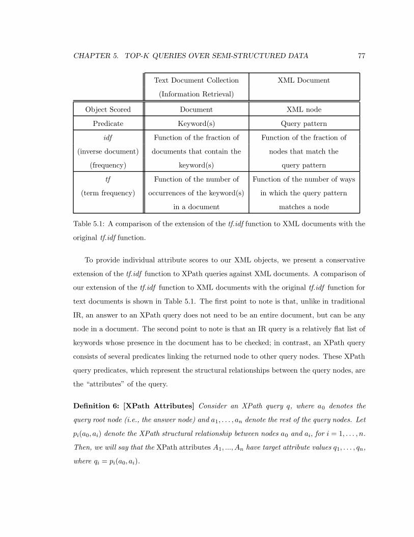
CHAPTER 5. TOP-K QUERIES OVER SEMI-STRUCTURED DATA 77
Text Document Collection XML Document
(Information Retrieval)
Object Scored Document XML node
Predicate Keyword(s) Query pattern
idf Function of the fraction of Function of the fraction of
(inverse document) documents that contain the nodes that match the
(frequency) keyword(s) query pattern
tf Function of the number of Function of the number of ways
(term frequency) occurrences of the keyword(s) in which the query pattern
in a document matches a node
Table 5.1: A comparison of the extension of the tf.idf function to XML documents with the
original tf.idf function.
To provide individual attribute scores to our XML objects, we present a conservative
extension of the tf.idf function to XPath queries against XML documents. A comparison of
our extension of the tf.idf function to XML documents with the original tf.idf function for
text documents is shown in Table 5.1. The first point to note is that, unlike in traditional
IR, an answer to an XPath query does not need to be an entire document, but can be any
node in a document. The second point to note is that an IR query is a relatively flat list of
keywords whose presence in the document has to be checked; in contrast, an XPath query
consists of several predicates linking the returned node to other query nodes. These XPath
query predicates, which represent the structural relationships between the query nodes, are
the “attributes” of the query.
Definition 6: [XPath Attributes] Consider an XPath query q, where a0 denotes the
query root node (i.e., the answer node) and a1, . . . , an denote the rest of the query nodes. Let
pi(a0, ai) denote the XPath structural relationship between nodes a0 and ai, for i = 1, . . . , n.
Then, we will say that the XPath attributes A1, ..., An have target attribute values q1, . . . , qn,
where qi = pi(a0, ai).

CHAPTER 5. TOP-K QUERIES OVER SEMI-STRUCTURED DATA 78
For example, the target values for the attributes of the XPath query of Figure 5.3(1) are
a[.//author="Dickens"], a[.//title="Great Expectations"] , and
a[./edition="paperback"]. The attributes provide a unique decomposition of the query
into a set of “atomic predicates”. This is akin to decomposing an IR keyword query into a
set of individual “keyword containment predicates”.
Definition 7: [XML IDF] Given a target attribute value qi for an XPath query, corre-
sponding to the XPath structural relationship pi(a0, ai), and an XML collection C, the idf
of qi against C, idf(qi, C), is given by:
log(1 +| {t ∈ C : tag(t) = a0} |
| {t ∈ C : tag(t) = a0 & (∃t′ ∈ C : tag(t′) = ai & p(t, t′) = qi))} |)
where p(t, t′) is the structural relationship between nodes t and t′. If there is no node t′ such
that p(t, t′) = qi then idf(qi, C) = 0.
Intuitively, the idf of target value qi against C quantifies the extent to which a0 nodes in the
collection C additionally satisfy pi(a0, ai). The fewer a0 nodes satisfy predicate pi(a0, ai),
the larger the idf of pi(a0, ai) is. This is analogous to the IR idf definition, where the fewer
documents contain a keyword k, the larger k’s idf is.
For example, consider Query (1) in Figure 5.3 and the collection C from Figure 2.1.
The predicates of the query are: descendant(book, title), descendant(book, author), and
child(book, edition). The idf scores of these predicates for the collection are:
idf(descendant(book, title), C) = log(1 + 3/3) = 0.301
idf(descendant(book, author), C) = log(1 + 3/3) = 0.301
idf(child(book, edition), C) = log(1 + 3/2) = 0.397
The idf scores of the first two predicates are equal to 0.301, which is the minimum possible
idf score of a predicate appearing in the collection, as the second term of the log is always at
least equal to 1 (all nodes satisfy the predicate). Since all three book nodes in the collection
satisfy the predicates, the predicates cannot be used to distinguish between book objects.
In contrast, since only one of the three fragments satisfies the third predicate, then the
corresponding idf score is greater than 0.301, and can be used to distinguish query answers.

CHAPTER 5. TOP-K QUERIES OVER SEMI-STRUCTURED DATA 79
Definition 8: [XML TF] Given a target attribute value qi for an XPath query, corre-
sponding to the XPath structural relationship pi(a0, ai), and an object t ∈ C with tag a0,
the tf of qi against object t, tf(qi, t), is given by:
| {t′ ∈ C : tag(t′) = ai & p(t, t′) = qi} |
where p(t, t′) is the structural relationship between nodes t and t′.
Intuitively, the tf of qi against object t quantifies the number of distinct ways in which t
satisfies predicate p. This is analogous to the IR tf definition, where the higher the number
of occurrences of a keyword k in a document d is, the larger the term frequency of k in d is.
In our XML collection from Figure 2.1, fragment (a) satisfies each predicate of Query
(1) once, and therefore has tf scores:
tf(descendant(book, title), a) = 1
tf(descendant(book, author), a) = 1
tf(child(book, edition), a) = 1
If fragment (a) had an additional edition child node under its book node, then its
tf(child(book,edition), a) would be equal to 2, giving higher scores to the object that
matches the query in more than one way.
Definition 9: [XML TF.IDF Score] Consider an XML collection C, a query q, and an
object t. Let qi be the target value of attribute Ai in q and let ti be the value of object t for
Ai. Then, the score of object t for attribute Ai, ScoreAi(qi, ti), is
ScoreAi(qi, ti) = idf(qi, C) · tf(qi, t)
The tf.idf scores of Query(1) over C for fragment (a) are then:
Scoretitle(descendant(book, title), a) = 0.301
Scoreauthor(descendant(book, author), a) = 0.301
Scoreedition(child(book, edition), a) = 0.397

CHAPTER 5. TOP-K QUERIES OVER SEMI-STRUCTURED DATA 80
The final score of fragment (a) for Query (1) is (0.301 + 0.301 + 0.397)/3 = 0.333. The
modified fragment (a) with one additional edition node would have a score of (0.301 +
0.301 + 0.794)/3 = 0.465. The scores of fragment (b) and (c) for Query (1) are both equal
to 0.2006. As expected, fragment (a), which matches Query (1), has higher score than the
approximate matches (b) and (c).
As defined, different exact answers to an XPath query may also receive different scores
if they have different tf scores. Therefore, an answer that matches query q in more distinct
ways will be assigned a higher score than another answer that does not have as many
ways to match q. Intuitively, this favors answers that are relevant to the query. This
is no different from the IR case of having different documents that contain each of the
query keywords having different scores. Once XPath query relaxations are permitted, an
approximate answer to the original query q is simply an exact answer to a relaxed query q ′
of q. Therefore, our tf.idf mechanism can also be used to score approximate answers to q.
Our data model for evaluating top-k queries over XML documents provides a mechanism
to return and score approximate matches to the queries. In particular, we designed a novel
scoring mechanism for approximate answers to XPath queries. In the rest of this chapter,
we discuss Whirlpool, a system to process top-k queries over XML data. Whirlpool uses our
extension of tf.idf to XML to score approximate answers to XPath queries.
5.3 The Whirlpool System
We now present Whirlpool, a system to evaluate top-k queries over heterogeneous XML
data. We start by describing the overall architecture of the Whirlpool system (Section 5.3.1).
Whirlpool adapts to a wide variety of query processing environments. We discuss the various
adaptive parameters of Whirlpool: prioritization strategies to select which object to process
next (Section 5.3.2), routing strategies to decide which attribute to evaluate on the selected
object (Section 5.3.3), and parallel alternatives to take advantage of the available parallelism
(Section 5.3.4).

CHAPTER 5. TOP-K QUERIES OVER SEMI-STRUCTURED DATA 81
5.3.1 Architecture
The Whirlpool approach permits different candidate answers to follow different query evalu-
ation plans, unlike traditional query processing strategies which select “global” query eval-
uation plans. In addition, at any given point in time, candidate answers may be at different
stages of the query execution. The per-answer query evaluation plans, as well as the answer
prioritization, are made during query execution based on the latest information available.
This flexibility in query processing is aimed at increasing pruning during query execution
to minimize the amount of work needed to return the top-k answers, and therefore reduce
query execution time.
������������
������� ���������������� � ���
�"! �$# �&% '(� ��)*�,+�-�. ��/0�1)��"! ��2*�034�*��� � ���
! 2�5 �6����� � ���
��7�! �$! ��26%$. )�.*���1�*)�/ �834����� � ���
)��9�":*���,% ;�! / �<��2 �034����� �*���
Figure 5.4: The Whirlpool architecture for the top-k query of Figure 5.1(ii).
The key components of the Whirlpool architecture are depicted in Figure 5.4, specialized
for the XPath query in Figure 5.1(ii) and its relaxations. The first components of Whirlpool
are servers and server queues. Servers are at the center of Whirlpool as they handle the
actual query evaluation. Specifically, each server evaluates the XML join (Definition 5)
corresponding to one attribute. Whirlpool is composed of one server per node in the XPath
tree pattern. Figure 5.4 shows the five servers for Query (ii), labeled with the query node
labels. Each of the other servers corresponds to a predicate in the XPath query, except for
the book server, which corresponds to the query root node. The root node server is slightly
different from the other servers as it is used to initialize the candidate answers (i.e., the

CHAPTER 5. TOP-K QUERIES OVER SEMI-STRUCTURED DATA 82
book nodes).
Predicate servers maintain a priority queue of objects to evaluate (none of which have
previously gone through this server). For each object at the head of its priority queue, a
server (i) computes, by performing an XML join operation (Definition 5), a set of spawned
objects, each of which extends the object with a server node (e.g., edition for the edition
server), if any, that is consistent with the structure of the query; (ii) computes scores for
each of the spawned object; (iii) determines if the spawned objects have an effect on the
top-k set; and (iv) decides whether each of the spawned objects can be pruned.
The join operations performed at each server should take two sources of complexity into
account:
• Query relaxations: Since Whirlpool allows for approximation in the query evaluation,
the join operation at the server should not only compute exact matches for the query
predicate associated with the server, but also compute all approximate matches cor-
responding to the query relaxations applied to the server predicate. In effect, the
server needs to check not only for the server predicate structural relationship, but
also possibly for some “relaxed” structural relationships present in the query.
For example, given the query in Figure 5.1(ii) and its Whirlpool architecture of Fig-
ure 5.4, the server corresponding to edition needs to check the predicate of the
form children(info, edition) for the exact query. Supporting edge generalization on
the edge (info, edition) would require checking for the predicate descendant(info,
edition). Allowing for subtree promotion on the subtree rooted at edition would
require checking for the predicate descendant(book, edition). Finally, the possibil-
ity of leaf node deletion means that the predicate comparing edition with book is
optional.
• Adaptive query processing: An evaluation strategy that relies on “global” query ex-
ecution plans guarantees that every object has been through the same number of
operations, in the same order. In an instantiation of Whirlpool for such a static strat-
egy, all the objects that arrive at a server have gone through exactly the same prior
server operations. An adaptive strategy allows for objects to go through different

CHAPTER 5. TOP-K QUERIES OVER SEMI-STRUCTURED DATA 83
sets of server operations. In an instantiation of Whirlpool for such an adaptive strat-
egy, objects that arrive at a server may have different sets of attribute values already
computed. For example, given the query in Figure 5.1(ii), objects arriving at the
edition server may have previously gone through any of the other servers. Check-
ing for query relaxations may require accessing some of the already present attribute
values. To evaluate an object at the edition server, we need to check the relation-
ship between the newly computed edition nodes and the object’s info attribute if
this attribute has already been computed. If the info attribute is unknown, then
the (info, edition) relationship will be checked when the object is evaluated by the
info server. Dealing with each of the exponential number of possible combinations
of already evaluated attributes separately would be inefficient from the point of view
of query processing.
We use the generateServerPredicates function shown in Figure 5.5 to generate the set
of predicates to be checked for an object arriving at each server. This function creates
the query relaxation predicates, as well as the extra predicates needed to consider all pos-
sible combinations of attributes present in an object. First, we look at the relationship
between the server node and the root node in the query, which we call structuralEdge in
Figure 5.5 (Step 2). If this relationship can be generalized (e.g., a child relationship can
be generalized to a descendant relationship), we insert the generalization first in the list of
server predicates Predicates (Step 3). We then insert structuralEdge in Predicates (Step
4). Then, we examine each node in the query tree and determine whether a relationship
(conditionalEdge) with the server node should be checked for that node (Steps 5–13). If
there is such a relationship, we first insert its generalization, if any, in Predicates (Steps
8 and 12), and then insert the relationship (Steps 9 and 13). By considering all possible
relationships between a query node and its ancestors and descendants in the tree, we are
able to effectively check for all possible combinations of edge generalization and subtree
promotion relaxations. The leaf deletion relaxation is taken into account by allowing the
server to output objects that have no matches for the server nodes, performing, in effect,
an outer-join [RG00].
As an example, for the edition server, the structuralEdge is descendant(book, edition).
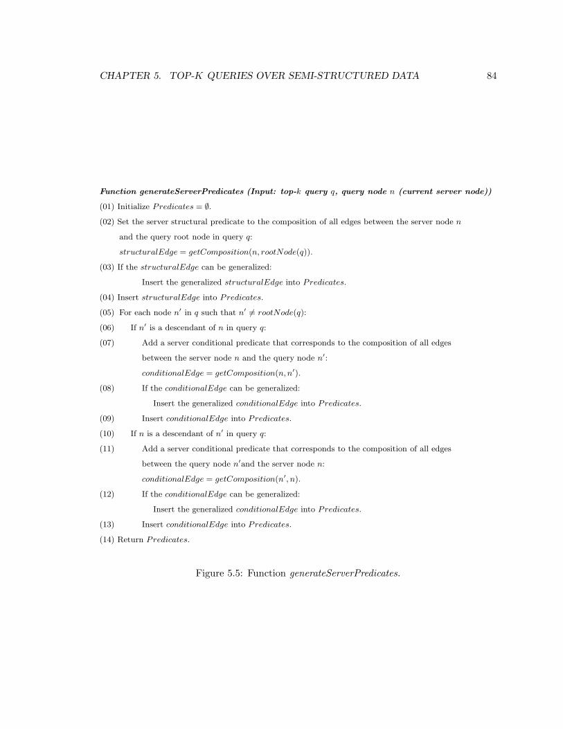
CHAPTER 5. TOP-K QUERIES OVER SEMI-STRUCTURED DATA 84
Function generateServerPredicates (Input: top-k query q, query node n (current server node))
(01) Initialize Predicates = ∅.
(02) Set the server structural predicate to the composition of all edges between the server node n
and the query root node in query q:
structuralEdge = getComposition(n, rootNode(q)).
(03) If the structuralEdge can be generalized:
Insert the generalized structuralEdge into Predicates.
(04) Insert structuralEdge into Predicates.
(05) For each node n′ in q such that n′ 6= rootNode(q):
(06) If n′ is a descendant of n in query q:
(07) Add a server conditional predicate that corresponds to the composition of all edges
between the server node n and the query node n′:
conditionalEdge = getComposition(n, n′).
(08) If the conditionalEdge can be generalized:
Insert the generalized conditionalEdge into Predicates.
(09) Insert conditionalEdge into Predicates.
(10) If n is a descendant of n′ in query q:
(11) Add a server conditional predicate that corresponds to the composition of all edges
between the query node n′and the server node n:
conditionalEdge = getComposition(n′, n).
(12) If the conditionalEdge can be generalized:
Insert the generalized conditionalEdge into Predicates.
(13) Insert conditionalEdge into Predicates.
(14) Return Predicates.
Figure 5.5: Function generateServerPredicates.
CHAPTER 5. TOP-K QUERIES OVER SEMI-STRUCTURED DATA 85
Since this edge cannot be generalized, it is inserted in Predicates. Then, the only node
for which edition has a relationship is info, with conditionalEdge child(info, edition).
Since this conditionalEdge can be generalized, we insert its generalization descendant(info,
edition) into Predicates before inserting the conditionalEdge child(info, edition) itself.
The predicates are used to efficiently evaluate objects at the server: the server first
locates all server nodes that match the first predicate in Predicates (structuralEdge).
Then, the actual object structure is refined by checking, in order, all of the relationships in
Predicates, allowing the server to compute the actual score of any objects it outputs.
The next component of Whirlpool is the top-k set (Figure 5.4), which contains the best
k objects, along with their scores. These objects may be partially evaluated, in which case
their scores may potentially increase as they are further evaluated, but will never decrease.
Only one instance of a given candidate answer may be present in the top-k set, although it
is possible for the system to evaluate several instantiations of the same candidate answer in
parallel (e.g., this could be the case if a candidate answer spawned several new candidate
answers at a server). When a server outputs an object, it checks the top-k set to determine
whether the object (i) updates the score of an existing match in the set, (ii) replaces an
existing match in the set, or (iii) is pruned (using Property 1) and hence it is not considered
further.
The final components of Whirlpool (Figure 5.4) are the router and the router queue,
which are used to determine to which server an object will be directed. The router queue
is prioritized using the maximum possible final scores of the objects (refer to Property 2
in Section 2.2.2). The router selects the object at the head of its queue, determines which
server will process the object next, and sends the object to the chosen server’s queue.
Whirlpool has reached an answer to the top-k query when no more objects are flowing
through the system, i.e., when all the queues are empty and neither the servers nor the
router are processing any objects.
Algorithm Whirlpool is shown in Figure 5.6. A few functions are worth highlighting
in this algorithm: sendToNextServer implements a routing decision (see Section 5.3.3 for
implementation alternatives), and computeJoinAtS computes the join predicates at a server.
Finally, updateTopK updates the top-k set by adding the input object to the top-k set, and

CHAPTER 5. TOP-K QUERIES OVER SEMI-STRUCTURED DATA 86
Algorithm Whirlpool (Input: top-k query q, k)
(01) Initialize topK = ∅, routerQueue = ∅, Candidates = rootNodes,
where rootNodes are all the nodes that match the query root node.
(02) For each node n′ in q:
(03) Initialize server s and its queue: s.queue = ∅,
generate the list of predicates for s: s.generateServerPredicates(q,n′).
(04) Add Candidates to routerQueue.
(05) While at least one of the router and server queues is not empty:
(06) If routerQueue not empty:
(07) Route the next object t′ in the routerQueue:
t′ = routerQueue.pop().
s = sendToNextServer(t′).
Insert t′ in s.queue.
(08) For each server s′ of q:
(09) Get the object t to process for s′: t = s.queue.pop().
(10) Perform the join operation at s′:
T = computeJoinAtS().
(11) For each object t′ in T (check t against the top-k set):
(12) If t′ is part of the best k objects: updateTopK(t′).
(13) If t′ can be pruned: discard t′.
(14) Else: insert t′ in routerQueue.
(15) Return topK.
Figure 5.6: Algorithm Whirlpool.
CHAPTER 5. TOP-K QUERIES OVER SEMI-STRUCTURED DATA 87
removing (if applicable) any object that does not belong to the top-k set any more.
In the next sections, we discuss the choices of strategies available in Whirlpool for the
queue prioritizations, routing decisions, and parallel alternatives.
5.3.2 Prioritization Strategies
When the router decides on a server to which to send an object, the object is inserted into
the server’s priority queue. The order in which objects are actually evaluated by the servers
depends on the prioritization strategy associated with the queue. We consider various
strategies for server prioritization:
• FIFO: The simplest alternative is to process objects in the order in which they were
inserted in the queue. This scheme is sensitive to the actual order in which objects are
processed, and performance may vary substantially depending on the order in which
objects are produced by the root server.
• Current score: Another alternative is to prioritize objects based on their current
(partial) scores, which is the minimum score that they are guaranteed to reach (i.e.,
their score lower bound). This scheme is sensitive to the order in which objects are
initially selected to be processed.
• Maximum possible next score: Another alternative is to prioritize objects based
on their expected scores after the next server operation. Assuming that we have per-
object estimates of the expected server increase, this scheme adapts to the score that
the current server could contribute to objects, making it less sensitive to the order in
which objects are processed.
• Maximum possible final score: A final alternative is to prioritize objects based on
their maximum possible final score (i.e., their score upper bound). This scheme is less
sensitive to the order in which objects are processed, and is the most adaptive of our
queue prioritization alternatives. Intuitively, this scheme enables those objects that
are highly likely to end up in the top-k set to be processed in a prioritized manner.

CHAPTER 5. TOP-K QUERIES OVER SEMI-STRUCTURED DATA 88
Our experimental results show that prioritizing both the server and router queues based
on the maximum possible final scores yields the best results. This is in line with our
observations from Section 2.2, and more specifically with Property 2, which states that the
object with the highest score upper bound will have to be processed before completing a
top-k answer in a sequential setting [MBG04, CH02]. In the remainder of this chapter,
results that we report for all our techniques assume server queues using maximum possible
final score prioritization strategies.
5.3.3 Routing Strategies
The router chooses the order in which servers evaluate objects. When an object arrives at
the router, many parameters are taken into account to decide which server is the best for
the object, and which execution plan will increase pruning the most. The router decides
which server, among those that have not yet evaluated the object, to choose based on one
of the following strategies:
• Static: The simplest alternative is to route each object through the same “global”
sequence of servers. For homogeneous data sets, this might actually be the strategy
of choice, where the sequence of servers can be determined a priori in a cost-based
manner.
• Score-based: Another alternative is to route the object to the server that is likely
to impact the object’s score the most. Two variations of this routing technique can
be considered: routing the object to the server that is likely to increase the object’s
score the most (max score), or the least (min score), based on some precomputed, or
estimated, information.
• Size-based: A final alternative is to route the object to the server that is likely to
produce the fewest spawned objects, taking into account the possible pruning after
checking the spawned objects against the top-k set. The intuition is that the overall
cost of the top-k query evaluation is a function of the number of objects that are
alive in the system. The size-based choice is a natural (simplified) adaptation for top-
k queries of conventional cost-based query optimization, and can be computed using
CHAPTER 5. TOP-K QUERIES OVER SEMI-STRUCTURED DATA 89
estimates of the number of spawned objects computed by the server for an object3, the
range of possible scores of these spawned objects, and the likelihood of these objects
getting pruned when compared against the top-k set.
In Section 5.4.2.1, we experimentally evaluate different object routing strategies for
Whirlpool.
5.3.4 Parallelism
As in our parallel web source scenario of Chapter 4, Whirlpool can take advantage of the
available parallelism of the system by using threads. Therefore, we consider the following
two instantiations of Whirlpool:
• Single-threaded: The simplest alternative is to have a single-threaded implemen-
tation of all the components in the system. This gives Whirlpool complete control
over which server is the next to process the object at the head of the server’s priority
queue.
• Multi-threaded: A more complex alternative is to allocate a thread (or more) to
each of the servers, as well as to the router, and let the system determine how to
schedule threads. Priority queues (Section 5.3.2) and adaptive routing strategies
(Section 5.3.3) are used to control the query evaluation. By using different threads,
Whirlpool is able to take advantage of available parallelism.
In Section 5.4.2.4, we experimentally evaluate both the single-threaded and the multi-
threaded versions of Whirlpool, on machines exhibiting different levels of parallelism.
5.4 Experimental Results
We now discuss the implementation of each component in the Whirlpool architecture (Sec-
tion 5.4.1), and present our experimental results for a range of architecture options and
query parameters (Section 5.4.2).
3Such estimates could be obtained by using work on selectivity estimation for XML.
CHAPTER 5. TOP-K QUERIES OVER SEMI-STRUCTURED DATA 90
5.4.1 Implementation
In this section, we describe in detail our implementation of the Whirlpool system. We
first present the XML top-k query processing techniques that we evaluate (Section 5.4.1.1).
Then, we define the data sets and queries for our evaluation (Section 5.4.1.2). Finally, we
describe our evaluation parameters (Section 5.4.1.3) and metrics (Section 5.4.1.4).
5.4.1.1 Techniques
Our experimental evaluation compare both the single- and multi-threaded instantiations of
Whirlpool with a traditional lock-step query evaluation approach. Specifically, we consider
the following three techniques:
Whirlpool-M: This is our multi-threaded variation of Whirlpool, where each server is
handled by an individual thread. In addition to server threads, a thread handles the router,
and the main thread checks for termination of top-k query execution.
Whirlpool-S: This is our single-threaded variation of Whirlpool. Due to the sequential
nature of Whirlpool-S, we slightly modified Whirlpool’s architecture (Figure 5.4) in our
implementation of Whirlpool-S: an object is processed by a server as soon as the object is
routed to the server; as a result the priority queues of the servers are not needed, and objects
are only kept in the router’s queue. Note that Whirlpool-S bears some similarities to both
Upper (Section 3.3) and MPro [CH02]. As in both techniques, objects are considered in the
order of their maximum possible final score (i.e., their score upper bound). In addition,
as in Upper, objects are routed to the server using an adaptive technique. While Upper
does not handle joins, MPro uses a join evaluation based on Cartesian products and on the
individual evaluation of each join predicate score. In contrast, our techniques use a different
model for evaluating joins where one single operation produces all valid join results at once.
LockStep: LockStep considers one server at a time and processes all objects sequentially
through a server before proceeding to the next server. Our default implementation of Lock-
Step keeps a top-k set based on the current scores of objects, and discards objects during
execution. We also considered a variation of LockStep without pruning during query exe-
cution, LockStep-NoPrun, where all object operations are performed, scores for all matches
are computed, and matches are then sorted at the end so that the k best matches can be
CHAPTER 5. TOP-K QUERIES OVER SEMI-STRUCTURED DATA 91
returned. Note that the LockStep algorithm is similar to the OptThres algorithm presented
in [AYCS02]. The relaxation adaptivity of OptThres, which decides whether an object
will be considered for relaxation depending on its score, is included in the default server
implementation of Whirlpool.
We implemented the three top-k query processing strategies in C++, using POSIX
threads for Whirlpool-M. We ran our experiments on a Red Hat 7.1 Linux 1.4GHz dual-
processor machine with a 2GB RAM and a Sun F15K running Solaris 8 with 54 CPUs
ranging from 900MHz to 1.2GHz, and 200GB of RAM.
5.4.1.2 Data and Queries
We generated several documents using the XMark document generating tool4. We then
manually created three queries by isolating XPath subsets of XMark queries that illustrate
the different relaxations.
• Q1: //item[./description/parlist]
• Q2: //item[./description/parlist and ./mailbox/mail/text]
• Q3: //item[./mailbox/mail/text[./bold and ./keyword] and ./name
and ./incategory]
Edge generalization is enabled by recursive nodes in the DTD (e.g., parlist). Leaf node
deletion is enabled by optional nodes in the DTD (e.g., incategory). Finally, subtree
promotion is enabled by shared nodes (e.g., text).
When a query is executed on an XML document, the document is parsed and nodes
involved in the query are stored in indexes along with their “Dewey” encoding5. Our server
implementation of XPath joins at each server uses a simple nested-loop algorithm based
on Dewey, since we are not comparing the performance of different join algorithms. We
discuss the effect of server operation time and its tradeoff with adaptive scheduling time in
Section 5.4.2.3. Scores for each match are computed using the scoring function presented
in Section 5.2.
4http://monetdb.cwi.nl/xml/index.html
5http://www.oclc.org/dewey/about/about the ddc.htm

CHAPTER 5. TOP-K QUERIES OVER SEMI-STRUCTURED DATA 92
Query Size Document Size k Parallelism Scoring Function
3 nodes (Q1), 1MB, 3, 1, 2, 4, ∞ sparse
6 nodes (Q2), 10MB, 15, dense
8 nodes (Q3) 50MB 75
Table 5.2: Evaluation parameters, with default values noted in boldface.
5.4.1.3 Evaluation Parameters
We measured the performance of our techniques for a variety of criteria, which are summa-
rized in Table 5.2:
• Query size: We consider queries of 3 nodes, 6 nodes, and 8 nodes (see Section 5.4.1.2).
The number of servers is equal to the number of nodes involved in a query. The number
of partial matches and thus the number of server operations for a top-k strategy is,
in the worst case, exponential in the number of nodes involved in the query.
• Document size: We consider XMark documents of sizes ranging from 1MB to 50MB.
• Value of k: We run experiments for values of k ranging from 3 to 75. When the value
of k increases, fewer partial matches can be pruned.
• Parallelism: Our Whirlpool-M approach can exploit the presence of multiple proces-
sors. We experiment with this strategy on different machines offering various levels
of parallelism, ranging from 1 to 48 processors.
• Scoring function: We use the tf.idf scoring function described in Section 5.2. We
observed that the tf.idf values generated for our XMark data set were skewed, with
some predicates having much higher scores than others. Given this behavior, we
decided to synthesize two types of scoring functions based on the tf.idf scores, to
simulate different types of data sets: sparse, where for each predicate, scores are
normalized between 0 and 1 to simulate data sets where predicate scores are uniform,
and dense, where score normalization is applied over all predicates to simulate data
sets where predicate scores are skewed. (The terms sparse and dense refer to the effect
CHAPTER 5. TOP-K QUERIES OVER SEMI-STRUCTURED DATA 93
of these functions on the distribution of final scores of objects.) We also experimented
with randomly generated sparse and dense scoring functions. A sparse function allows
for a few objects to have very high scores, resulting in high k − th score values, which
enables more pruning. With a dense scoring function, the final scores of objects are
close to each other, resulting in less pruning. Using different scoring functions permits
to study the impact of score distribution on our performance measures.
5.4.1.4 Evaluation Metrics
To compare the performance of the different techniques, we use the following metrics:
• Query Execution Time: This is the overall time needed to return the top-k answers.
This measure gives us the performance of the various techniques.
• Number of Server Operations: This is the total number of join operations performed
by all servers. This measure allows us to evaluate the actual workload of the various
techniques, regardless of parallelism.
• Number of Objects Created: This is the total number of partial answers created during
query evaluation. This measure gives us an intuition of how good a technique is at
pruning objects during query execution.
5.4.2 Experiments
We now present experimental results for our top-k query evaluation algorithms. We first
study various adaptive routing strategies (Section 5.4.2.1) and settle on the most promising
one. We then compare adaptive and static strategies (Section 5.4.2.2), and show that
adaptive routing outperforms static routing when the server operation cost dominates in
the query execution time, and that lock-step strategies always perform worse than strategies
that let partial matches progress at different rates (Section 5.4.2.3). We study the impact
of parallelism (Section 5.4.2.4) and of our evaluation parameters (Section 5.4.2.5) on our
adaptive techniques. Finally, we discuss scalability (Section 5.4.2.6).
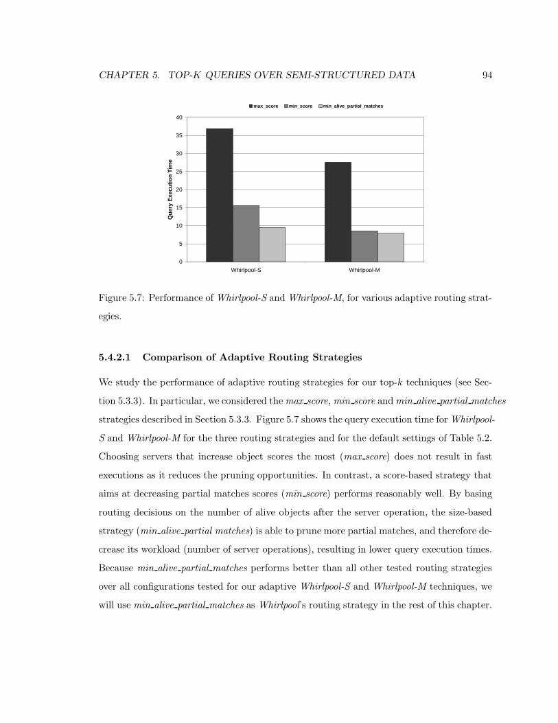
CHAPTER 5. TOP-K QUERIES OVER SEMI-STRUCTURED DATA 94
0
5
10
15
20
25
30
35
40
Whirlpool-S Whirlpool-M
Qu
ery
Exe
cuti
on
Tim
e
max_score min_score min_alive_partial_matches
Figure 5.7: Performance of Whirlpool-S and Whirlpool-M, for various adaptive routing strat-
egies.
5.4.2.1 Comparison of Adaptive Routing Strategies
We study the performance of adaptive routing strategies for our top-k techniques (see Sec-
tion 5.3.3). In particular, we considered the max score, min score and min alive partial matches
strategies described in Section 5.3.3. Figure 5.7 shows the query execution time for Whirlpool-
S and Whirlpool-M for the three routing strategies and for the default settings of Table 5.2.
Choosing servers that increase object scores the most (max score) does not result in fast
executions as it reduces the pruning opportunities. In contrast, a score-based strategy that
aims at decreasing partial matches scores (min score) performs reasonably well. By basing
routing decisions on the number of alive objects after the server operation, the size-based
strategy (min alive partial matches) is able to prune more partial matches, and therefore de-
crease its workload (number of server operations), resulting in lower query execution times.
Because min alive partial matches performs better than all other tested routing strategies
over all configurations tested for our adaptive Whirlpool-S and Whirlpool-M techniques, we
will use min alive partial matches as Whirlpool’s routing strategy in the rest of this chapter.

CHAPTER 5. TOP-K QUERIES OVER SEMI-STRUCTURED DATA 95
0
10
20
30
40
50
60
70
80
90
100
LockStep-NoPrun LockStep Whirlpool-S Whirlpool-M
Qu
ery
Exe
cuti
on
Tim
e (i
n s
eco
nd
s)
max(STATIC) median(STATIC) min(STATIC) ADAPTIVE
Figure 5.8: Performance of LockStep-NoPrun, LockStep, Whirlpool-S and Whirlpool-M, for
static and adaptive routing strategies (linear scale).
0
5000
10000
15000
20000
25000
30000
LockStep Whirlpool-S Whirlpool-M
Nu
mb
er o
f S
erve
r O
per
atio
ns
max(STATIC) median(STATIC) min(STATIC) ADAPTIVE
Figure 5.9: Number of server operations for LockStep, Whirlpool-S and Whirlpool-M, for
static and adaptive routing strategies (linear scale).

CHAPTER 5. TOP-K QUERIES OVER SEMI-STRUCTURED DATA 96
5.4.2.2 Adaptive vs. Static Routing Strategies
We now compare adaptive routing strategies against static ones. Figures 5.8 and 5.9 show
the query execution time and the number of server operations needed for Whirlpool-S and
Whirlpool-M, as well as for both LockStep and LockStep-NoPrun using the default values
in Table 5.2. For all techniques, we considered all (120) possible permutations of the static
routing strategy, where all objects go through the servers in the same order. In addition,
for Whirlpool-S and Whirlpool-M, we considered our adaptive strategy (see Section 5.4.2.1).
For both LockStep strategies, all objects have to go through one server before the next server
is considered; LockStep is thus static by nature. This implementation of LockStep is similar
to the OptThres algorithm presented in [AYCS02].
For all techniques, we report the minimum, maximum and median values for the static
routing strategy. A perfect query optimizer would choose the query plan that results in
the minimum value of the static routing strategy. Figures 5.8 and 5.9 show that, for
a given static routing strategy, Whirlpool-M is faster than Whirlpool-S, which in turn is
faster than LockStep. Thus, allowing some objects to progress faster than others, by letting
them being processed earlier by more servers, results in savings in query execution time
and total number of server operations. The no-pruning version of LockStep is worse than
all other techniques, proving the benefits of pruning when processing top-k queries. In
addition, for both Whirlpool-S and Whirlpool-M, our adaptive routing strategy results in
query executions that are at least as efficient as the best of the static strategies. (For dense
scoring functions, adaptive routing strategies resulted in much better performance than the
best static strategy.) Interestingly, for this default setting, Whirlpool-M performs slightly
more server operations than Whirlpool-S. However, the better performance of Whirlpool-M
is due to its use of parallelism (two processors are available on our default machine) to
speed up query processing time.
Since Whirlpool always outperforms LockStep, and Whirlpool’s adaptive routing strategy
performs as well as or better than its static one, we will only consider the adaptive routing
versions of Whirlpool-S and Whirlpool-M in the rest of this chapter. The terms Whirlpool-S
and Whirlpool-M will now refer to their adaptive versions.
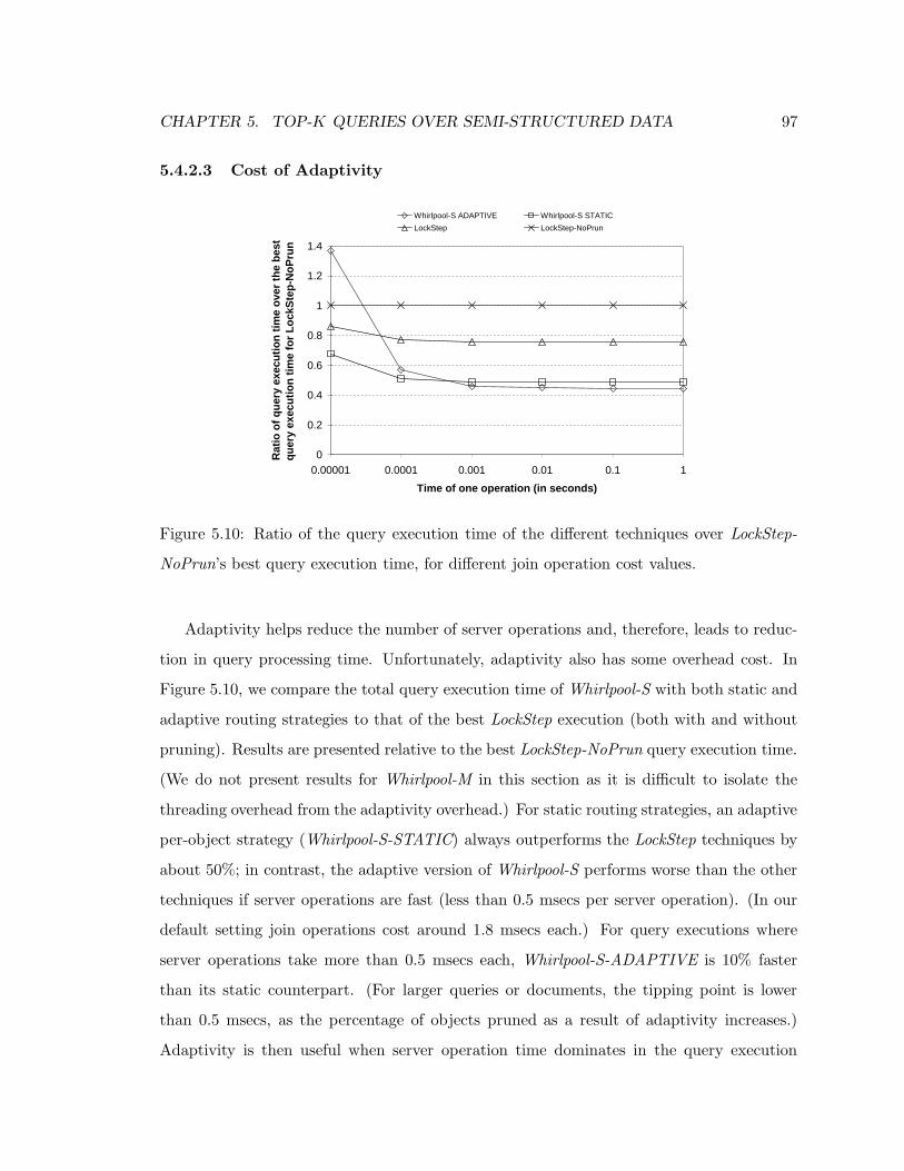
CHAPTER 5. TOP-K QUERIES OVER SEMI-STRUCTURED DATA 97
5.4.2.3 Cost of Adaptivity
0
0.2
0.4
0.6
0.8
1
1.2
1.4
0.00001 0.0001 0.001 0.01 0.1 1
Time of one operation (in seconds)
Rat
io o
f q
uer
y ex
ecu
tio
n t
ime
ove
r th
e b
est
qu
ery
exec
uti
on
tim
e fo
r L
ock
Ste
p-N
oP
run
Whirlpool-S ADAPTIVE Whirlpool-S STATIC
LockStep LockStep-NoPrun
Figure 5.10: Ratio of the query execution time of the different techniques over LockStep-
NoPrun’s best query execution time, for different join operation cost values.
Adaptivity helps reduce the number of server operations and, therefore, leads to reduc-
tion in query processing time. Unfortunately, adaptivity also has some overhead cost. In
Figure 5.10, we compare the total query execution time of Whirlpool-S with both static and
adaptive routing strategies to that of the best LockStep execution (both with and without
pruning). Results are presented relative to the best LockStep-NoPrun query execution time.
(We do not present results for Whirlpool-M in this section as it is difficult to isolate the
threading overhead from the adaptivity overhead.) For static routing strategies, an adaptive
per-object strategy (Whirlpool-S-STATIC) always outperforms the LockStep techniques by
about 50%; in contrast, the adaptive version of Whirlpool-S performs worse than the other
techniques if server operations are fast (less than 0.5 msecs per server operation). (In our
default setting join operations cost around 1.8 msecs each.) For query executions where
server operations take more than 0.5 msecs each, Whirlpool-S-ADAPTIVE is 10% faster
than its static counterpart. (For larger queries or documents, the tipping point is lower
than 0.5 msecs, as the percentage of objects pruned as a result of adaptivity increases.)
Adaptivity is then useful when server operation time dominates in the query execution
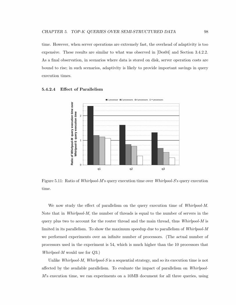
CHAPTER 5. TOP-K QUERIES OVER SEMI-STRUCTURED DATA 98
time. However, when server operations are extremely fast, the overhead of adaptivity is too
expensive. These results are similar to what was observed in [Des04] and Section 3.4.2.2.
As a final observation, in scenarios where data is stored on disk, server operation costs are
bound to rise; in such scenarios, adaptivity is likely to provide important savings in query
execution times.
5.4.2.4 Effect of Parallelism
0
1
2
q1 q2 q3
Rat
io o
f W
hir
lpo
ol-
M q
uer
y ex
ecu
tio
n t
ime
ove
r W
hir
lpo
ol-
S q
uer
y ex
ecu
tio
n t
ime
1 processor 2 processors 4 processors � processors
Figure 5.11: Ratio of Whirlpool-M’s query execution time over Whirlpool-S’s query execution
time.
We now study the effect of parallelism on the query execution time of Whirlpool-M.
Note that in Whirlpool-M, the number of threads is equal to the number of servers in the
query plus two to account for the router thread and the main thread, thus Whirlpool-M is
limited in its parallelism. To show the maximum speedup due to parallelism of Whirlpool-M
we performed experiments over an infinite number of processors. (The actual number of
processors used in the experiment is 54, which is much higher than the 10 processors that
Whirlpool-M would use for Q3.)
Unlike Whirlpool-M, Whirlpool-S is a sequential strategy, and so its execution time is not
affected by the available parallelism. To evaluate the impact of parallelism on Whirlpool-
M’s execution time, we ran experiments on a 10MB document for all three queries, using
CHAPTER 5. TOP-K QUERIES OVER SEMI-STRUCTURED DATA 99
15 as the value for k, on four different machines with 1, 2, 4, and ∞ processors.6 We then
computed the speedup of Whirlpool-M over the execution time of Whirlpool-S, and report
our results in Figure 5.11. When there is no parallelism (i.e., when the number of available
processors is equal to one) the performance of Whirlpool-M compared to that of Whirlpool-S
depends on the query size: Whirlpool-M can take more than twice the time of Whirlpool-S
for small queries, but becomes faster when parallelism is available for large queries. When
multiple processors are available, Whirlpool-M becomes faster than Whirlpool-S, up to 1.5
times faster with two processors, up to 1.95 times faster with four processors, and up to a
maximum of almost 3.5 times faster when the number of available processors is unlimited.
For Q1, Whirlpool-M is not faster than Whirlpool-S, even when parallelism is available, as
Q1 only has three servers and does not take as much advantage of parallelism as Q2 and
Q3 do, making the threading overhead expensive in comparison to the gains of parallelism.
In addition, Q1 is evaluated faster than Q2 and Q3, and is thus penalized more strongly by
the threading overhead. For Q2 and Q3, Whirlpool-M takes advantage of parallelism, with
better results for the larger Q3 than for Q2.
The speedup stops increasing when the number of processors exceeds the number of
threads needed to evaluate the query. Our example queries do not take advantage of paral-
lelism greater than the number of servers involved in the query plus two to account for the
router and main threads. Thus Q1 does not benefit from having more than 5 processors,
Q2 from more than 8 processors, and Q3 from more than 10 processors. If more parallelism
is available, we could create several threads for the same server, thus increasing parallelism
even further.
5.4.2.5 Varying Evaluation Parameters
We now study the effect of our parameters from Section 5.4.1.3.
Varying Query Size: Figure 5.12 shows the query execution time for both Whirlpool-S
and Whirlpool-M for our three sample queries (Table 5.2), on a logarithmic scale. The
query execution time grows exponentially with the query size. Because of the logarithmic
scale, the differences between Whirlpool-S and Whirlpool-M are larger than they appear on
6Our 4-processor machine is actually a dual Xeon machine with four “logical” processors.

CHAPTER 5. TOP-K QUERIES OVER SEMI-STRUCTURED DATA 100
0.1
1
10
100
1000
K=3 K=15 K=75 K=3 K=15 K=75 K=3 K=15 K=75
q1 q2 q3
Qu
ery
Exe
cuti
on
Tim
e
Whirlpool-M Whirlpool-S
Figure 5.12: Performance of Whirlpool-S and Whirlpool-M, as a function of k and the query
size (logarithmic scale).
the plot. The difference between Whirlpool-M and Whirlpool-S in terms of query execution
time increases with the size of the query, with Whirlpool-S being 20% faster for Q1 and
Whirlpool-M being 48% faster for Q3 (k=15), since the threading overhead has less impact
on larger queries.
Varying k: Figure 5.12 reports the effect of varying the number of matches returned in
the top-k answer. The query execution time is linear with respect to k. Interestingly, the
difference in query execution time between Whirlpool-S and Whirlpool-M increases with k.
This increase is more significant for larger query sizes, and Whirlpool-M is up to 60% faster
than Whirlpool-S for Q3 and for k=75. The number of server operations exhibits a similar
behavior (although at a smaller scale), with 8% fewer server operation for Whirlpool-M
for the Q3, k=75 setting. This is rather counter-intuitive: [CH02] proved that sequen-
tial top-k algorithms based on probing the object with the highest possible final score, as
does Whirlpool-S, minimizes the total number of operations with respect to a given routing
strategy. Our algorithms of Chapters 3 and 4 use a similar intuition (see Property 2 in Sec-
tion 2.2.2), although they are not proven to minimize the total number of operations as they
aim at minimizing the query execution time. Since our implementations of Whirlpool-S and

CHAPTER 5. TOP-K QUERIES OVER SEMI-STRUCTURED DATA 101
Whirlpool-M use the same routing strategy, Whirlpool-S should always perform fewer server
operations. The explanation lies in our adaptive routing strategy: min alive partial matches
relies on score estimates, server selectivity, and current top-k values to make its choice. This
last parameter, current top-k values, changes during query execution. From monitoring the
executions of Whirlpool-S and Whirlpool-M, we observed that top-k values grow faster in
Whirlpool-M than in Whirlpool-S, which may lead to different routing choices for the same
object. This in turn makes the algorithms follow, in effect, different schedules for the same
object. By making better routing choices, Whirlpool-M results in fewer objects being created
than Whirlpool-S.
0.01
0.1
1
10
100
1000
10000
1M 10M 50M 1M 10M 50M 1M 10M 50M
q1 q2 q3
Qu
ery
Exe
cuti
on
Tim
e
Whirlpool-M Whirlpool-S
Figure 5.13: Performance of Whirlpool-S and Whirlpool-M, as a function of the document
and query sizes (logarithmic scale, k=15).
Varying Document Size: Figure 5.13 reports on the effect of the XML document size
on the query execution time. The execution time grows exponentially with the document
size; the larger the document, the more objects will have to be evaluated, resulting in
more server operations and thus longer query execution times. For a small document, the
result is quite fast (less than 1.2 sec for all queries tested), making the thread overhead in
Whirlpool-M expensive compared to Whirlpool-S’s execution time. However, for medium
and large documents, Whirlpool-M becomes up to 92% faster than Whirlpool-S (Q2, 50 MB

CHAPTER 5. TOP-K QUERIES OVER SEMI-STRUCTURED DATA 102
Document Size 1MB 10MB 50MB
Q1 100% 93.12% 85.66%
Q2 100% 49.56% 57.66%
Q3 100% 39.59% 31.20%
Table 5.3: Percentage of objects created by Whirlpool-M, as a function of the maximum
possible number of objects, for different query and document sizes.
document, k=15).
Varying Scoring Function: We experimented with different scoring functions, namely
with both sparse and dense variations of the tf.idf scoring function, as well as with randomly
generated scoring functions that were designed to have either dense or sparse properties.
We observed that sparse scoring functions lead to faster query execution times (due to
faster pruning). In contrast, with dense scoring functions, the relative differences between
Whirlpool-M and Whirlpool-S are greater, with Whirlpool-M resulting in greater savings in
terms of query processing time, and number of server operations and objects created, over
Whirlpool-S.
5.4.2.6 Scalability
A top-k query processing technique over XML documents has to deal with the explosion of
objects that occurs when query and document sizes increase. To measure the scalability of
Whirlpool, we considered the number of objects created during query execution as a fraction
of the maximum possible number of such objects. The total number of objects is obtained
by running an algorithm with no pruning, namely LockStep-NoPrun. Table 5.3 shows that
the percentage of total possible objects created by Whirlpool-M significantly decreases with
the document and query sizes. The benefits of pruning are modest for small queries. While
all objects are created for Q1, for which objects generated by the root server do not create
“spawned” objects in the join servers, pruning allows to reduce the number of operations of
these partial objects. For large queries (Q3), Whirlpool-M evaluates fewer than 40% of the
objects on the 10MB document, and fewer than 32% on the 50MB document. By pruning
CHAPTER 5. TOP-K QUERIES OVER SEMI-STRUCTURED DATA 103
objects based on score information, Whirlpool-M and Whirlpool-S exhibit good scalability
in both query and document size.
5.5 Conclusions
In this chapter, we presented Whirlpool, an adaptive evaluation strategy for computing ex-
act and approximate top-k answers for XPath queries. Our results showed that adaptivity
is very appropriate for top-k queries in XML. We observed that the best adaptive strat-
egy focuses on minimizing the intermediate number of alive objects; this is analogous to
traditional query optimization in RDBMS, where the focus is on minimizing intermediate
table sizes. By letting partial matches progress at different rates, Whirlpool results in faster
query execution times than non-adaptive top-k query processing techniques. In addition,
Whirlpool scales well when query and document sizes increase. While we do not focus on
evaluating XPath scoring functions, we show that Whirlpool adapts itself to environments
where scores of intermediate answers are either sparse or dense. We studied the effect of
parallelism on our Whirlpool approaches and observed that, although Whirlpool-M is better
for most cases, when parallelism is not available or if query or document size is small, the
Whirlpool-M threading overhead may hurt performance. In contrast, for large queries and
documents, Whirlpool-M exploits the available parallelism and results in significant savings
in query execution time over Whirlpool-S.
Chapter 6 104
Chapter 6
Extensions to the Top-k Query
Model
Our top-k query processing algorithms of the previous chapters are designed for scenarios
where all of the query attributes are part of the ranking criteria, and where the top-k answers
are single objects. In addition, our techniques return the exact top-k query answers. In
this chapter, we extend our query processing algorithms of the previous chapters to handle
natural variations of the basic top-k query model of Chapter 2. For simplicity, we focus on
the model and algorithms of Chapters 3 and 4; however, the adaptations presented in this
chapter could be easily extended to the model and algorithms of Chapter 5.
As a first step, we extend our query model to handle more complex query scenarios.
Specifically, we consider, in addition to fuzzy attribute preferences, some hard Boolean
constraints on attributes. Our new query model, therefore, contains both the ranking
expressions of Chapter 2 and some filtering conditions on the objects, and is similar to the
query model of [CG96, CGM04].
Example 3: Consider our restaurant example from Chapter 2. Let Cuisine be another
attribute of restaurants, in addition to the Address, Price, and Rating attributes defined in
Example 1. If a user is interested only in “French” restaurants, then a query for the top-3
restaurants should be a list of the three restaurants that match the user Address, Price, and
Rating specifications the closest, and for which the Cuisine attribute has the value “French”.
CHAPTER 6. EXTENSIONS TO THE TOP-K QUERY MODEL 105
As this example suggests, an object whose attribute value does not match a filtering con-
dition should be discarded regardless of its score for the ranking component of the query.
For instance, an “Italian” restaurant close to the user-input address, with high rating and
price around $25, is not an acceptable answer for the above query.
In addition to filtering conditions, we also consider an extension to our query model
to handle scenarios where individual objects can be combined through join operations. In
such scenarios, we are interested in combining information from different sources, to return
more complex objects as query answers.
Example 4: Consider again our restaurant example from Chapter 2. A user is now in-
terested in getting recommendations for an evening out, including a dinner and a movie.
Consider a recommendation service providing information on the restaurants (as detailed
in Example 1), the movie theaters, and the movies that are available. In addition to the
restaurant preferences of Example 1, the user is interested in a highly rated movie (“Re-
view”=10) that plays at an inexpensive theater (“Ticket”=$5) that happens to be close to
the restaurant of choice. An answer to such a top-3 query should be a list of (restaurants,
theater, movie) triplets that are closest to the user-specified preferences.
In Section 6.1, we consider these extensions to our query model of Chapter 2, and discuss
appropriate variations of our algorithms of Chapters 3 and 4.
Finally, we have so far focused on algorithms that return the exact k best matches
for a query efficiently. Interestingly, to improve efficiency further we might want to return
approximate top-k answers in some cases, without seriously compromising the quality of the
query results. In effect, the top-k query model presupposes that query answers are flexible
by nature, so allowing for some extra flexibility to gain efficiency might be desirable. In
Section 6.2, we develop extensions of our algorithms for this approximate top-k query model.
In this chapter, we make the following contributions:
• An extension of our query model from Chapter 2 that captures more complex web
data scenarios.
• An experimental evaluation of suitable adaptations of our algorithms from Chapters 3
and 4 to this more complex query model.
CHAPTER 6. EXTENSIONS TO THE TOP-K QUERY MODEL 106
• A framework to allow our algorithms to return approximate top-k query answers in
exchange for faster query executions.
• An experimental evaluation of the adaptations of our algorithms from Chapters 3
and 4 to the approximate top-k query framework.
The rest of this chapter is organized as follows. First, we extend our web-scenario query
model and algorithms to handle more complex query scenarios in Section 6.1. Then, in
Section 6.2, we discuss a top-k query approximation framework and adapt our algorithms
to this framework. Finally, we conclude this chapter in Section 6.3.
6.1 Top-k Query Processing Strategies over Web Sources
We now extend our query model of Chapter 2 to handle more complex query scenarios such
as the ones described in Examples 3 and 4. In Section 6.1.1, we adapt our algorithms of
Chapters 3 and 4 to handle Boolean filtering conditions. In Section 6.1.2, we adapt our
algorithms of Chapters 3 and 4 to a multi-object scenario involving joins.
6.1.1 Filtering Conditions
We extend our model to consider Boolean filtering conditions on attributes. The filtering
conditions in our framework are similar to a selection operator in a relational algebra.
Filtering conditions result in additional pruning of objects during top-k query evaluation,
thus their possible effects must be taken into account when pruning objects based on score
information.
Consider a collection C of objects with attributes A1, . . . , An, plus perhaps some other
attributes not mentioned in our queries. A top-k query over collection C simply specifies
target values for each ranking attribute Ai, for i = 1, . . . ,m, as well as a Boolean condition
value on each filtering attribute Aj, for j = m + 1, . . . , n. Therefore, a top-k query is an
assignment of values {A1 = q1, . . . , An = qn} to the attributes of interest.
Example 3 (cont.): Consider our restaurant example. Our top-3 query in this example
assigns a target value to all three restaurant ranking attributes, namely “2590 Broadway”
CHAPTER 6. EXTENSIONS TO THE TOP-K QUERY MODEL 107
for Address, $25 for Price, and 30 for Rating, as well as a filtering value, “French,” for
attribute Cuisine.
The answer to a top-k query q = {A1 = q1, . . . , An = qn} over a collection of objects
C and for a scoring function is a list of k objects in the collection with the highest score
for the query. The score that each object t in C receives for q is generally a function of
ScoreAi(qi, ti), the score for each individual ranking attribute Ai, for i = 1, . . . ,m, of t, and
of ScoreAj(qj, tj), the score for each individual filtering attribute Aj , for j = m+1, . . . , n, of
t, where qi is the target value of attribute Ai in the query and ti is the value of object t for
Ai. For ranking attributes, this score is defined as in Chapter 2. For filtering attributes, this
score is equal to 1 if the attribute values satisfy the filtering condition, and to 0 otherwise.
Example 3 (cont.): A restaurant object r has a score of 1 for the Cuisine attribute and
for the above query if r’s cuisine type is “French”; in contrast, if r’s cuisine type is not
“French” then r’s score for Cuisine is 0.
The final score of an object is then
Score(q, t) =
0 if ∃i, i = m + 1, . . . , n such that si = 0∑m
i=1 wi · si otherwise
where si = ScoreAi(qi, ti), and wi is the weight of Ai in q. We use this scoring function in our
algorithms of Sections 6.1.1.1 and 6.1.1.2. We report experimental results on adaptations
of our algorithms of Chapter 3 and 4 to this query model in Section 6.1.1.3.
6.1.1.1 Sequential Algorithms
In this section, we adapt the sequential algorithms of Chapter 3 to a top-k query model
where both ranking expressions and filtering conditions are present in the queries.
The adaptation of TA (Section 3.2.1) is straightforward, as TA does not make any dy-
namic choices during query processing. To adapt TAz-EP (Section 3.2.2), we must consider
the effect of filtering conditions on object scores and take these into account when ordering
attribute accesses. Since a filtering attribute can by itself give enough information to dis-
card an object (namely, if its score is 0), we always start by accessing filtering attributes
CHAPTER 6. EXTENSIONS TO THE TOP-K QUERY MODEL 108
on an object, and then consider ranking attributes in Rank order (see Section 3.2.2). In
the presence of statistics on the expected selectivity of filtering conditions, we order the
filtering attributes in decreasing order of selectivity.
To adapt Upper, we need to take into account the filtering conditions when deciding
which source to access for a selected object. However, the choice of object to process
next does not depend on filtering conditions as it is based only on the current score upper
bounds of the objects. Therefore, the main Upper algorithm of Figure 3.3 is unchanged, and
the SelectBestSource function, which handles source selection, is modified to take filtering
conditions into account. To adapt the SelectBestSource function, we need to be able to
efficiently compare for each object the effect of probing each ranking and filtering attribute.
For this purpose, we assign a filtering probability to every attribute of an object t:
• A filtering attribute’s filtering probability is equal to the selectivity of the filtering
condition associated with that attribute.
• A ranking attribute’s filtering probability is equal to the likelihood that object t will
be discarded after the ranking attribute is accessed. We expect t to be discarded if
U(t) < score′k, where score′k is the k-th largest expected object score. Assuming that
attribute scores are distributed uniformly, we can define the filtering probability of a
ranking attribute Ai as
Filtering Probability(Ai) =1 −
score′k
wi
tR(Ri),
where wi is the weight of attribute Ai in the query (Section 2.1) and tR(Ri) is the
random-access time of source Ri (Section 3.1).
To estimate score′k, we need to take into consideration the possibility that some of
the k objects with the current largest expected object score may be discarded through
filtering conditions. Therefore, we assign to each object t a filter value that represents
the probability that this object will not be discarded through filtering conditions. This
value is then equal to the product of the selectivities of the not-yet probed filtering
attributes of t, and is equal to 1 if all filtering attributes of t have been probed and
have not discarded t. The value of score′k is then the expected value of the k′-th
CHAPTER 6. EXTENSIONS TO THE TOP-K QUERY MODEL 109
object with largest expected score, where k ′ is obtained by adding the filter values
of objects in decreasing order of expected score values, and choosing object k ′ as the
object that brings this sum to a value of k.
The modified SelectBestSource function always returns the source with the largest fil-
tering probability for object t.
6.1.1.2 Parallel Algorithms
We now adapt the parallel algorithms of Chapter 4 to a top-k query model where both
ranking expressions and filtering conditions are present in the query.
The adaptation of pTA (Section 4.2) to this query model is trivial: pTA does not make
per-object choices, but sends objects to sources in the order in which they are discovered.
Therefore, the adaptation of pTA to a scenario with both ranking and filtering attributes
is identical to the original pTA of Section 4.2.
The pUpper algorithm (Section 4.3) relies on the SelectBestSubset function to make
per-object decisions on which source to probe. We adapt the SelectBestSubset function to
take into account our filtering probabilities of Section 6.1.1.1. Specifically, the modified Se-
lectBestSubset function picks, for a given object t, the fastest subset of sources taking source
congestion into account (Section 4.3.2) that is expected to discard t with probability greater
than a threshold value. This threshold value is a parameter of the algorithm. We conducted
experiments for various threshold values and report on the results in Section 6.1.1.3.
6.1.1.3 Experimental Results
We now report on experimental results for both the sequential (Section 6.1.1.1) and the
parallel (Section 6.1.1.2) adaptations of our top-k query processing algorithms for a query
model with filtering conditions and ranking expressions.
In this section, we use the default experimental settings of Sections 3.4.1 and 4.4.1. To
isolate the effect of filtering conditions on the query executions, we only consider scenarios
with one sorted-access source. In addition, our default implementation considers attributes
to be evenly divided between filtering and ranking attributes.

CHAPTER 6. EXTENSIONS TO THE TOP-K QUERY MODEL 110
0
10000
20000
30000
40000
50000
60000
70000
80000
90000
100000
Uniform Gaussian Zipfian Correlated Mixed Cover
t pro
bes
TAz-EP-FilterFirst UpperUpper-FilterFirst Upper-Filtering
Figure 6.1: Performance of the sequential strategies for the default setting of the experiment
parameters, and for alternate attribute-value distributions.
0
10000
20000
30000
40000
50000
60000
70000
80000
90000
100000
0 1 2 3 4 5 6
Number of filtering attributes
t pro
bes
TAz-EP-FilterFirst UpperUpper-FilterFirst Upper-Filtering
Figure 6.2: Performance of the sequential strategies for the default setting of the experiment
parameters, as a function of the number of filtering attributes.
CHAPTER 6. EXTENSIONS TO THE TOP-K QUERY MODEL 111
Sequential Strategies: Figures 6.1 and 6.2 show experimental results for our sequential
algorithms of Section 6.1.1.1. Specifically, we compare the executions of TAz-EP-FilterFirst,
our adaptation of TAz-EP; Upper-Filtering, our adaptation of Upper; the original Upper
algorithm of Section 3.3; and Upper-FilterFirst, an adaptation of Upper that, like TAz-EP-
FilterFirst, always probes filtering attributes first and then accesses ranking attributes in
Rank order. Figure 6.1 shows the performance of the four techniques, in probing time, for
the local data sets of Section 3.4.1.3. Our results show that Upper-Filtering consistently
outperforms the other techniques. Upper, which does not consider filtering conditions to
make its choices, has the worst overall performance. Finally, Upper-FilterFirst, while not
as good as Upper-Filtering, consistently exhibits probing times slightly lower than that
of TAz-EP-FilterFirst: while both techniques share the same per-object source selection
strategy, Upper-FilterFirst benefits from interleaving probes on objects. Figure 6.2 shows
the performance of the four techniques when the number of filtering attributes varies (out
of six attributes). Upper-Filtering is the best strategy when there is at least one filtering
attribute. The results confirm that Upper is the best strategy for the query model of
Chapter 3, where no filtering attributes are present.
Parallel Strategies: Figures 6.3 and 6.4 show experimental results for our parallel al-
gorithms of Section 6.1.1.2. Specifically, we compare the executions of pTA; pUpper-Filter,
our adaptation of pUpper, with threshold values of 0 and 0.25; and the original pUpper al-
gorithm of Section 4.3. Figure 6.3 shows the performance of the four techniques, in probing
time, for the local data sets of Section 3.4.1.3. Our results show that pUpper-Filter with
a threshold value of 0 consistently outperforms the other techniques. This suggests that
pUpper-Filter gives better performance when only one attribute per object is selected by
the SelectBestSubset function (i.e., when the subsets are of size 1). pUpper has performance
close to the best version of pUpper-Filter. Figure 6.4 shows the performance of the four tech-
niques when the number of filtering attributes varies (out of six attributes). Upper-Filter
with threshold value of 0 is the best strategy for all configurations. Surprisingly, pUpper-
Filter is the best strategy for the query model of Chapter 4, where no filtering attributes
are present. Results for different data distributions for a query model with no filtering

CHAPTER 6. EXTENSIONS TO THE TOP-K QUERY MODEL 112
0
1000
2000
3000
4000
5000
6000
7000
8000
9000
10000
Uniform Gaussian Zipfian Correlated Mixed Cover
t pro
bes
pTA pUpper
pUpper-Filter-0 pUpper-Filter-0.25
Figure 6.3: Performance of the parallel strategies for the default setting of the experiment
parameters, and for alternate attribute-value distributions.
0
1000
2000
3000
4000
5000
6000
7000
8000
0 1 2 3 4 5 6 7
Number of filtering attributes
t pro
bes
pTA pUpper
pUpper-Filter-0 pUpper-Filter-0.25
Figure 6.4: Performance of the parallel strategies for the default setting of the experiment
parameters, as a function of the number of filtering attributes.
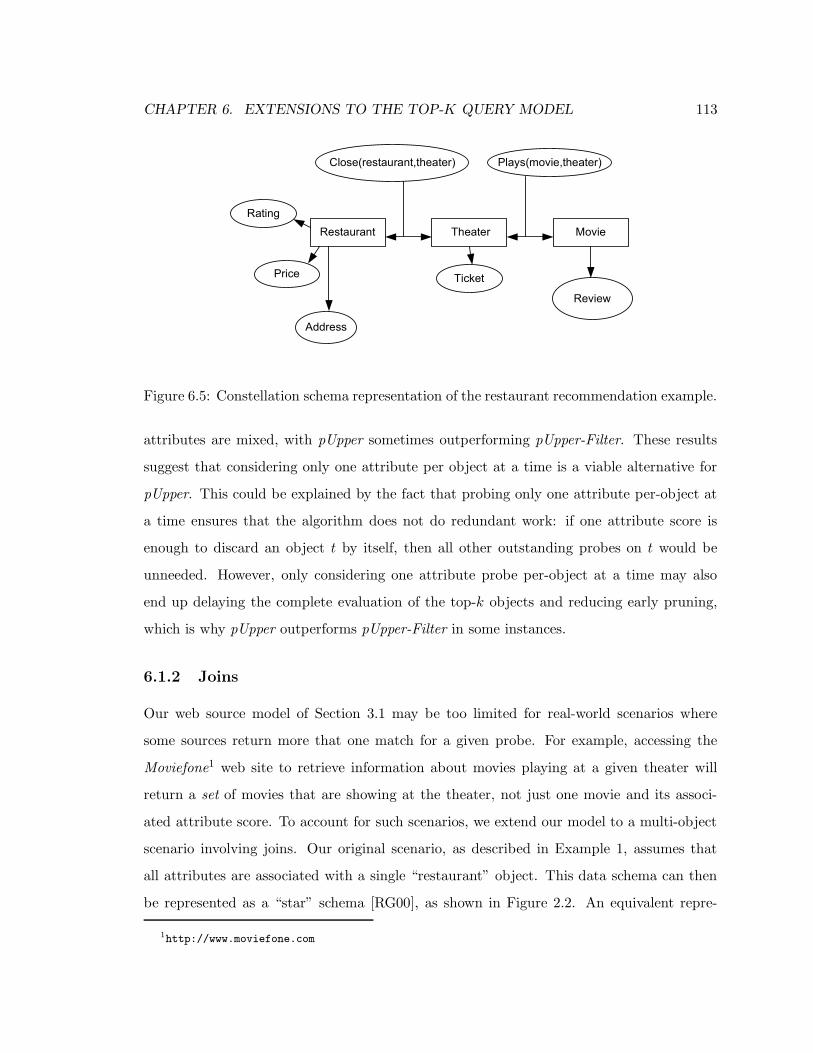
CHAPTER 6. EXTENSIONS TO THE TOP-K QUERY MODEL 113
������������� ���
�����
������
�����
����
�����
��� ���� ��������� ��� ������������
Figure 6.5: Constellation schema representation of the restaurant recommendation example.
attributes are mixed, with pUpper sometimes outperforming pUpper-Filter. These results
suggest that considering only one attribute per object at a time is a viable alternative for
pUpper. This could be explained by the fact that probing only one attribute per-object at
a time ensures that the algorithm does not do redundant work: if one attribute score is
enough to discard an object t by itself, then all other outstanding probes on t would be
unneeded. However, only considering one attribute probe per-object at a time may also
end up delaying the complete evaluation of the top-k objects and reducing early pruning,
which is why pUpper outperforms pUpper-Filter in some instances.
6.1.2 Joins
Our web source model of Section 3.1 may be too limited for real-world scenarios where
some sources return more that one match for a given probe. For example, accessing the
Moviefone1 web site to retrieve information about movies playing at a given theater will
return a set of movies that are showing at the theater, not just one movie and its associ-
ated attribute score. To account for such scenarios, we extend our model to a multi-object
scenario involving joins. Our original scenario, as described in Example 1, assumes that
all attributes are associated with a single “restaurant” object. This data schema can then
be represented as a “star” schema [RG00], as shown in Figure 2.2. An equivalent repre-
1http://www.moviefone.com
CHAPTER 6. EXTENSIONS TO THE TOP-K QUERY MODEL 114
sentation in the relational model would be a single table, with all restaurant information.
Our multi-object scenario, as described in Example 4, considers several objects, “restau-
rant”, “theater”, and “movie”. Each object has one or more associated attributes. A top-k
query answer is then a combination of the objects of the query; this is a triplet (restaurant,
theater, movie) in Example 4. The score of a top-k query answer over this multi-object
data model is a weighted sum of all the attributes of the objects involved in the answer.
This data schema can then be represented as a “constellation” schema [RG00], as shown in
Figure 6.5. An equivalent representation in the relational model would be multiple tables,
each one of them containing information on different objects.
In this section, we augment our source model definition of Section 3.1 (Definition 1)
with the following source type:
Definition 10: [C-Source] Consider an attribute Ai, an object t, and a top-k query q.
Assume further that Ai is handled by a source S. We say that S is a C-Source if we can
obtain from S a set of objects oj , j = 1, . . . , l, along with their ScoreAiby invocation of
a getObjects(S, q, t) probe interface. The ScoreAivalue for a return object oj is the join
score of t and oj and is determined by the value of both objects. As for R-Sources, we refer
to the average time that it takes S to return a set of objects along with their scores for a
given object as tR(S).
Example 4 (cont.): Consider our (restaurant, theater, movie) example. A set of movies
playing at a theater h are provided by the Moviefone web site, which also provides informa-
tion about the time the movies are shown. Hence, Moviefone is a C-Source. The objects
returned by an access to Moviefone are the set of (h, movie) pairs, where the score of the
Plays attribute, which corresponds to the movie time, is determined by the values of h and
each individual movie object.
An access to a C-Source is, in effect, a join operation and thus leads to the creation
of new candidate answers whenever accessed. As in our XML scenario of Chapter 5, a
challenging aspect of efficient top-k query processing in our multi-object scenario is then to
minimize the explosion in the number of candidate answers to reduce the amount of work
needed to reach a top-k answer.

CHAPTER 6. EXTENSIONS TO THE TOP-K QUERY MODEL 115
Next, we adapt our sequential and parallel algorithms of Chapters 3 and 4 to our multi-
object query model, in Sections 6.1.2.1 and 6.1.2.2, respectively. We then present experi-
mental results in Section 6.1.2.3.
6.1.2.1 Sequential Algorithms
In this section, we adapt the sequential algorithms of Chapter 3 to our multi-object top-k
query model.
The adaptation of TA (Section 3.2.1) is straightforward, as TA does not make any dy-
namic choices during query processing. To adapt TAz-EP (Section 3.2.2), we must consider
the effect of joins on object scores and on the number of candidate answers. We consider
two alternate adaptive measures to make per-object dynamic choices:
• Score-based: We consider the impact of each not-yet-probed attribute on the object
score. This measure is similar to the Rank measure used in Section 3.2.2 with one
notable difference: some attributes may not be directly accessible through a single
probe. For instance, in Example 4, from a restaurant object, we need to access first
the theater object before being able to probe the Ticket, Plays, and Review attributes.
When making a dynamic choice on which attribute to access next, we can only consider
those attributes that are currently accessible. However, since an attribute Ai may
permit accesses to other attributes, the Rank measure takes into account the sum of
the expected decrease of U(t) after probing Si, the source corresponding to attribute
Ai, and the expected decrease of U(t) after probing all sources that will be directly
accessible after accessing Si.
• Size-based: We consider the impact of each not-yet-probed attribute on the number
of candidate answers. This measure is similar to the min alive partial matches strat-
egies described in Section 5.3.3 and is defined as the inverse of the expected number
of candidate answers created by accessing the attribute divided by the source-access
cost. We estimate the expected number of candidate answers created by a C-Source
access using selectivity statistics; for an R-Source, the expected number of candidate
answers created is always one.
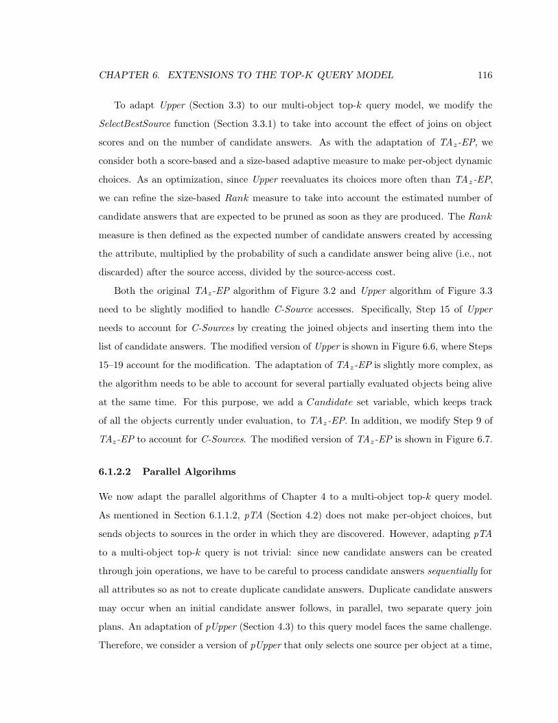
CHAPTER 6. EXTENSIONS TO THE TOP-K QUERY MODEL 116
To adapt Upper (Section 3.3) to our multi-object top-k query model, we modify the
SelectBestSource function (Section 3.3.1) to take into account the effect of joins on object
scores and on the number of candidate answers. As with the adaptation of TAz-EP, we
consider both a score-based and a size-based adaptive measure to make per-object dynamic
choices. As an optimization, since Upper reevaluates its choices more often than TAz-EP,
we can refine the size-based Rank measure to take into account the estimated number of
candidate answers that are expected to be pruned as soon as they are produced. The Rank
measure is then defined as the expected number of candidate answers created by accessing
the attribute, multiplied by the probability of such a candidate answer being alive (i.e., not
discarded) after the source access, divided by the source-access cost.
Both the original TAz-EP algorithm of Figure 3.2 and Upper algorithm of Figure 3.3
need to be slightly modified to handle C-Source accesses. Specifically, Step 15 of Upper
needs to account for C-Sources by creating the joined objects and inserting them into the
list of candidate answers. The modified version of Upper is shown in Figure 6.6, where Steps
15–19 account for the modification. The adaptation of TAz-EP is slightly more complex, as
the algorithm needs to be able to account for several partially evaluated objects being alive
at the same time. For this purpose, we add a Candidate set variable, which keeps track
of all the objects currently under evaluation, to TAz-EP. In addition, we modify Step 9 of
TAz-EP to account for C-Sources. The modified version of TAz-EP is shown in Figure 6.7.
6.1.2.2 Parallel Algorihms
We now adapt the parallel algorithms of Chapter 4 to a multi-object top-k query model.
As mentioned in Section 6.1.1.2, pTA (Section 4.2) does not make per-object choices, but
sends objects to sources in the order in which they are discovered. However, adapting pTA
to a multi-object top-k query is not trivial: since new candidate answers can be created
through join operations, we have to be careful to process candidate answers sequentially for
all attributes so as not to create duplicate candidate answers. Duplicate candidate answers
may occur when an initial candidate answer follows, in parallel, two separate query join
plans. An adaptation of pUpper (Section 4.3) to this query model faces the same challenge.
Therefore, we consider a version of pUpper that only selects one source per object at a time,

CHAPTER 6. EXTENSIONS TO THE TOP-K QUERY MODEL 117
Algorithm Upper (Input: top-k query q)
(01) Initialize Uunseen = 1, Candidates = ∅, and returned = 0.
(02) While (returned < k)
(03) If Candidates 6= ∅, pick tH ∈ Candidates such that U(tH) = maxt∈Candidates U(t).
(04) Else tH is undefined.
(05) If tH is undefined or U(tH) < Uunseen (unseen objects might have larger scores than
all candidates):
(06) Use a round-robin policy to choose the next SR-Source Di (1 ≤ i ≤ nsr) to access
via a sorted access.
(07) Get the best unretrieved object t from Di: t← getNext(Di, q).
(08) Update Uunseen = ScoreComb(s`(1), . . . , s`(nsr), 1, . . . , 1| {z }
nr times
),
where s`(j) is the last score seen under sorted access in Dj . (Initially, s`(j) = 1.)
(09) If t /∈ Candidates: Insert t in Candidates.
(10) Else If tH is completely probed (tH is one of the top-k objects):
(11) Return tH with its score; remove tH from Candidates.
(12) returned = returned + 1.
(13) Else:
(14) Di ← SelectBestSource(tH ,Candidates).
(15) If Di is an R-Source:
(16) Retrieve tH ’s score for attribute Ai, si, via a random probe to Di:
si ← getScore(Di, q, tH).
(17) If Di is a C-Source:
(18) Retrieve the objects spawned from tH via a probe to Di:
O ← getObjects(Di, q, tH).
(19) While O 6= ∅:
Retrieve an object o from O. Insert o into Candidates.
Figure 6.6: Adaptation of the Upper algorithm for the join scenario.
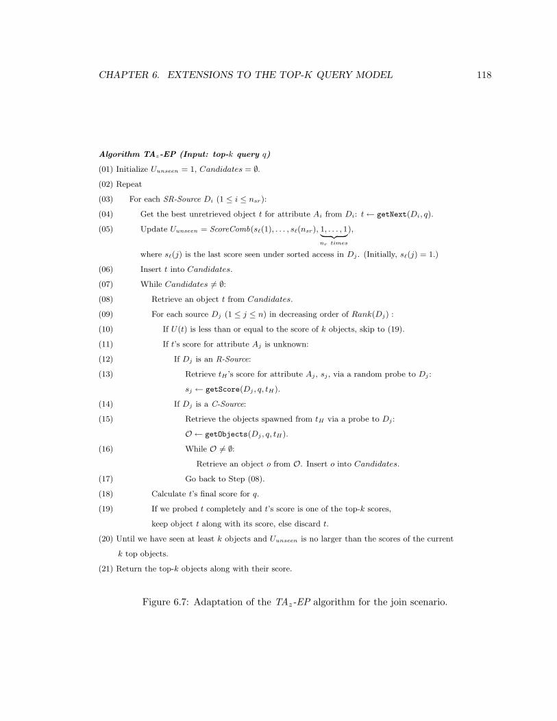
CHAPTER 6. EXTENSIONS TO THE TOP-K QUERY MODEL 118
Algorithm TAz-EP (Input: top-k query q)
(01) Initialize Uunseen = 1, Candidates = ∅.
(02) Repeat
(03) For each SR-Source Di (1 ≤ i ≤ nsr):
(04) Get the best unretrieved object t for attribute Ai from Di: t← getNext(Di, q).
(05) Update Uunseen = ScoreComb(s`(1), . . . , s`(nsr), 1, . . . , 1| {z }
nr times
),
where s`(j) is the last score seen under sorted access in Dj . (Initially, s`(j) = 1.)
(06) Insert t into Candidates.
(07) While Candidates 6= ∅:
(08) Retrieve an object t from Candidates.
(09) For each source Dj (1 ≤ j ≤ n) in decreasing order of Rank(Dj) :
(10) If U(t) is less than or equal to the score of k objects, skip to (19).
(11) If t’s score for attribute Aj is unknown:
(12) If Dj is an R-Source:
(13) Retrieve tH ’s score for attribute Aj , sj , via a random probe to Dj :
sj ← getScore(Dj , q, tH).
(14) If Dj is a C-Source:
(15) Retrieve the objects spawned from tH via a probe to Dj :
O ← getObjects(Dj , q, tH).
(16) While O 6= ∅:
Retrieve an object o from O. Insert o into Candidates.
(17) Go back to Step (08).
(18) Calculate t’s final score for q.
(19) If we probed t completely and t’s score is one of the top-k scores,
keep object t along with its score, else discard t.
(20) Until we have seen at least k objects and Uunseen is no larger than the scores of the current
k top objects.
(21) Return the top-k objects along with their score.
Figure 6.7: Adaptation of the TAz-EP algorithm for the join scenario.

CHAPTER 6. EXTENSIONS TO THE TOP-K QUERY MODEL 119
Function SelectBestSubset (Input: object t)
(1) Choose source Di (1 ≤ i ≤ n) such that
(i) Di is not yet probed for t, and
(ii) Rank(Di) = max(Rank(Dj)) among all Dj (1 ≤ j ≤ n) sources not yet probed for t.
(2) Return Di.
Figure 6.8: Adaptation of the SelectBestSubset function for the join scenario.
in effect modifying the SelectBestSubset function to produce subsets containing only one
source. The natural adaptation of pTA to the multi-object query model is then identical to
the adaptation of pUpper as in both cases we only select one source per object. We consider
two alternatives for selecting the source for a given object: score-based and size-based, as
defined in Section 6.1.2.1. The modified version of the SelectBestSource function is shown in
Figure 6.8. For the score-based version of pUpper, the Rank metric for a source Di is defined
as Rank(Di) = Wi
eR(Di), where Wi is the sum of all δ values, as defined in Section 3.2.2, for
Di as well as for all sources that will be directly accessible after accessing Di, and eR(Di)
is the expected access time of Di as defined in Section 4.3.2. For the sized-based version of
pUpper, the Rank metric for a source Di is defined as Rank(Di) = Ni
eR(Di), where Ni is the
inverse of the expected number of candidate answers created by accessing Di, and eR(Di)
is the expected access time of Di.
6.1.2.3 Experimental Results
We now report the experimental results for both the sequential (Section 6.1.2.1) and parallel
(Section 6.1.2.2) adaptations of our top-k query processing algorithms for a multi-object
query model.
In this section, we use the default experimental settings of Sections 3.4.1 and 4.4.1. To
isolate the effect of multiple objects on the query executions, we only consider scenarios
with one sorted-access source. In addition, to show the effect of the presence of both C-
Sources and R-Sources, we consider a three-object query as our default query (i.e., our
default setting consists of three C-Sources and three S-Sources). Finally, to show the effect
of an increase in the number of candidate answers, we set the default selectivity of the join

CHAPTER 6. EXTENSIONS TO THE TOP-K QUERY MODEL 120
operations performed at the C-Sources to three, which means that the expected number of
candidate answers spawned by a C-Source access is three.
0
100000
200000
300000
400000
500000
600000
Uniform Gaussian Zipfian Correlated Mixed Cover
t pro
bes
TAz-EP-Score TAz-EP-Size
Upper-Score Upper-Size
Figure 6.9: Performance of the sequential strategies for the default setting of the experiment
parameters, and for alternate attribute-value distributions.
Sequential Strategies: Figures 6.9 through 6.12 show experimental results for our se-
quential algorithms of Section 6.1.2.1. Specifically, we compare the executions of TAz-
EP-Score, our adaptation of TAz (Section 3.2.2) that uses a score-based decision strategy;
TAz-EP-Size, our adaptation of TAz that uses a size-based decision strategy; Upper-Score,
our adaptation of Upper (Section 3.3) that uses a score-based decision strategy; and Upper-
Size, our adaptation of Upper that uses a size-based decision strategy. Figure 6.9 shows the
performance of the four techniques, in probing time, for the local data sets of Section 3.4.1.3.
The techniques that base their choices on size perform better than their score-based counter-
parts, which confirms our observation of Chapter 5. For the Cover data set, the score-based
techniques are significantly worse than the size-based techniques. This is due to the fact
that the actual expected attribute scores in the Cover data sets are very different from the
default value of 0.5 used by our score-based techniques when the actual expected score is
unknown.

CHAPTER 6. EXTENSIONS TO THE TOP-K QUERY MODEL 121
0
100000
200000
300000
400000
500000
600000
700000
0 1 2 3 4 5 6 7
Number of Query Objects
t pro
bes
TAz-EP-Score TAz-EP-Size
Upper-Score Upper-Size
Figure 6.10: Performance of the sequential strategies for the default setting of the experi-
ment parameters, as a function of the number of query objects (centralized schema).
0
100000
200000
300000
400000
500000
600000
700000
800000
0 1 2 3 4 5 6 7
TAz-EP-Score TAz-EP-Size
Upper-Score Upper-Size
Figure 6.11: Performance of the sequential strategies for the default setting of the experi-
ment parameters, as a function of the number of query objects (chained schema).
CHAPTER 6. EXTENSIONS TO THE TOP-K QUERY MODEL 122
0
200000
400000
600000
800000
1000000
1200000
1400000
1600000
1800000
0 2 4 6 8 10 12
Join Selectivity
t pro
bes
TAz-EP-Score TAz-EP-Size
Upper-Score Upper-Size
Figure 6.12: Performance of the sequential strategies for the default setting of the experi-
ment parameters, as a function of the join selectivity.
Figures 6.10 and 6.11 show the performance of the techniques when the number of
query objects varies. We considered two possible schema representation of the query ob-
jects: centralized, where all query objects are accessible through only one C-Source access;
and chained, where query objects need to be accessed sequentially (e.g., in our restaurant
example, we need to access the theaters before being able to access the movies). The results
are similar to those of Figure 6.9. When only one query object is present, the query model
is similar to that of Chapter 3, and, as expected, the score-based techniques outperform
the size-based techniques. When there is more than one query object, size-based techniques
have the best performance. Finally, Figure 6.12 shows the performance of the four tech-
niques when the query selectivity (represented by the expected number of objects created by
a join operation) varies. The difference in performance between size-based and score-based
techniques increases with the join selectivity, confirming that a size-based approach is the
best strategy in the presence of joins.

CHAPTER 6. EXTENSIONS TO THE TOP-K QUERY MODEL 123
Parallel Strategies: Figures 6.13 and 6.14 show experimental results for our parallel
algorithms of Section 6.1.2.1. Specifically, we compare the executions of pUpper-Score, our
adaptation of pUpper (Section 4.3) that uses a score-based decision strategy; and pUpper-
Size, our adaptation of pUpper that uses a size-based decision strategy. Figure 6.13 shows the
performance of the four techniques, in probing time, for the local data sets of Section 3.4.1.3,
and Figure 6.14 shows the performance on the techniques as a function of the number
of query objects, for a centralized query schema. Surprisingly, pUpper-Score consistently
outperforms pUpper-Size. This can be explained by the precomputation step of pUpper:
unlike sequential techniques, which are immediately penalized by the increase in the number
of candidate answers resulting from a join, pUpper does not consider newly created candidate
answers until its next call to GenerateQueues (Figure 4.4 in Section 4.3.3). Since score-
based strategies allow for faster pruning based on scores, pUpper-Score can benefit from
this additional pruning, without being penalized for choosing sources that increase the
number of candidate answers.
0
10000
20000
30000
40000
50000
60000
70000
80000
90000
100000
Uniform Gaussian Zipfian Correlated Mixed Cover
t pro
bes
pUpper-Score pUpper-Size
Figure 6.13: Performance of the parallel strategies for the default setting of the experiment
parameters, and for alternate attribute-value distributions.

CHAPTER 6. EXTENSIONS TO THE TOP-K QUERY MODEL 124
0
2000
4000
6000
8000
10000
12000
0 1 2 3 4 5 6 7
Number of Query Objects
t pro
bes
pUpper-Score pUpper-Size
Figure 6.14: Performance of the parallel strategies for the default setting of the experiment
parameters, as a function of the number of query objects (centralized schema).
6.2 Approximate Evaluation of Top-k Queries
In the previous section, we extended our query model to handle a broader range of web
scenarios. In addition, we might be willing to trade quality in the top-k query answer for
speedup in query processing time. In effect, the top-k query model presupposes that query
answers are flexible by nature, so allowing for some extra flexibility to gain efficiency might
be desirable.
In this section, we present some adaptations of our algorithms of Chapters 3 and 4 to
handle approximation in top-k query processing. In Section 6.2.1, we extend our top-k
query model and present some answer quality metrics for approximate query processing.
In Section 6.2.2, we adapt our algorithms to take a user-specified approximation tolerance
as input. In Section 6.2.3, we present some “online” approximation algorithms that return
information on the status of the query executions at regular intervals. We show some
experimental evaluation of the various approximation techniques, and present a visualization
tool for our approximate top-k techniques in Section 6.2.4.

CHAPTER 6. EXTENSIONS TO THE TOP-K QUERY MODEL 125
6.2.1 Approximation Model and Metrics
The query and data model for our approximate algorithms is similar to that of Chapter 2
and of Sections 3.1 and 4.1 (for parallel executions). However, in an approximate top-k
query scenario, query execution may stop before the exact top-k objects are identified in
exchange for faster query executions. The algorithms presented in the previous chapters
return exact top-k answers, thus the answer quality is always perfect. To evaluate the loss
of quality of approximate top-k answers, we can use the following metrics:
• Precision: This represents the percentage of (approximate) top-k objects returned for
a query that are actual top-k objects for the query. A similar approximation metric
was suggested in [CH02].
• θ-approximation: An approximate top-k query answer is a θ-approximation of the
exact query answer if no object that is not in the approximate top-k answer can have
a final score higher than (1 + θ) · scorek, where scorek is the lowest object score in
the approximate top-k solution. This approximation metric allows for early stopping
of the algorithms when the current top-k objects are “good enough” with respect to
θ. This θ-approximation was first suggested in [FLN03].
6.2.2 User-Defined Approximation
We adapt the top-k query processing algorithms from Chapters 3 and 4 to provide an
approximate top-k answer within a user-defined tolerance, which corresponds to the decrease
in solution quality that is acceptable in exchange for faster executions. The user-defined
tolerance value is a parameter of the approximate algorithm and should be given before
query execution.
We adapt algorithms from Chapters 3 and 4 to the approximate query scenario using
the θ-approximation approach introduced in [FLN03]. We modify the algorithms to stop
when the score of the current top-k objects according to score upper bounds are within the
user-specified approximation tolerance θ from the score upper bounds of the other objects.
In other words, we stop when (1 + θ)Lk ≥ Ucandidates, where Lk is the score lower bound of
the k current top objects (sorted by score lower bounds), and Ucandidates is the score upper
CHAPTER 6. EXTENSIONS TO THE TOP-K QUERY MODEL 126
bound of objects not in the top-k set. We rewrite Property 1 (Section 2.2) to account for
this θ-approximation:
Property 3: Consider a top-k query q and suppose that, at some point in time, we have
retrieved and partially evaluated a set of objects for the query. Assume further that, for an
object t, U(t) < (1 + θ)L(ti), for k different objects t1, . . . , tk ∈ T . Then t can safely be
discarded under the θ-approximation assumption for q.
Specifically, we modify Steps 7 and 12 in TAz-EP (Figure 3.2) to take the θ-approximation
into account in the condition. Similarly, we modify the condition in Step 5 of Upper (Fig-
ure 3.3). Finally, in pUpper (Figure 4.3), we modify Step 12 to take into account the
θ-approximation.
This approach is not incremental, in the sense that once query execution has started,
the approximation value cannot be decreased without having to restart the whole query
execution. Some objects whose final scores are higher than the θ-approximate objects might
be discarded if their score upper bounds are lower than (1 + θ)Lk at anytime during query
execution. However, these objects might not have been discarded if θ had been lower, and
could be part of a tighter approximation of the top-k query. For instance, some of the exact
top-k objects might be discarded during the evaluation of a θ-approximate top-k query; if θ
is decreased to 0 (exact answer requested) later, the information on these objects would be
lost. Thus, unless the implementation keeps track of all discarded objects, the query will
have to be restarted to give results with a lower approximation value.
We report experiments on the quality/time tradeoff of θ-approximation in Section 6.2.4.2.
6.2.3 Online Approximation
In our second approach, the top-k query processing algorithms from Chapters 3 and 4 are
processed as if they were to return the exact top-k solution. At regular intervals during
query processing, the current query state as well as some approximation quality measures
are returned to the user, in the spirit of online query processing [HHW97, RH02]. The user
can decide online whether to wait for more refined query results or to stop query processing
and use the current answer.
CHAPTER 6. EXTENSIONS TO THE TOP-K QUERY MODEL 127
For such online top-k processing strategies, it is important to provide an approximation
metric that gives some intuition about how far the processing is from reaching an exact
solution. Such a metric should be a monotonically decreasing function that becomes 0
when the top-k solution is reached.
We considered several distance functions and chose the following function for our “dis-
tance to solution” metric: D = Uall − Lk, where Uall is the highest score upper bound of
all objects that are not completely probed, and Lk is the k-th highest score lower bound.
Since Uall cannot increase and Lk cannot decrease during query execution, then D has the
required monotonicity qualities. In addition, D can be computed efficiently at run time as
it only requires keeping track of the k objects with the highest score lower bounds, as well
as maintaining a priority queue of objects based on their score upper bounds. We describe
how to efficiently maintain object-score information in [GMB02]. The other functions that
we considered either were not monotonic or required accessing all the objects. An example
function is the sum of undiscarded object “ranges”, where an object range is the difference
between its score upper bound and its score lower bound; using this function would result
in important local execution time overhead.
We report experiments on the changes in answer quality during query processing using
online approximation in Section 6.2.4.3.
6.2.4 Experimental Results
In this section, we present our implementation choices, evaluation parameters, and metrics
(Section 6.2.4.1). We report experimental results for the user-defined approximation (Sec-
tion 6.2.4.2) and the online approximation adaptation (Section 6.2.4.3) of our algorithms of
Chapters 3 and 4. In addition, we describe our implementation of a visualization interface
for our techniques (Section 6.2.4.4).
6.2.4.1 Implementation
We implemented the approximation techniques on top of the existing C++ implementation
of our algorithms, and evaluated them using the local data sources of Section 3.4.1.3.
CHAPTER 6. EXTENSIONS TO THE TOP-K QUERY MODEL 128
Techniques: We compare the performance of adaptations to our approximate query sce-
nario of the sequential Upper (Section 3.3) and TAz-EP (Section 3.2) techniques, as well
as the parallel pUpper (Section 4.3) and pTA (Section 4.2) techniques. To adapt these
techniques to the θ-approximation scenario, we modified some conditions in the algorithms,
as described in Section 6.2.2. For the online approximation scenario, we used the original
algorithms as introduced in Chapters 3 and 4, and regularly interrupted the execution to
retrieve the values of our online approximation measures.
Evaluation Parameters: For the θ-approximation scenario, we report results for differ-
ent values of the θ-approximation. For the online approximation scenario, we report results
of the query execution at regular intervals, as measured by the probing time tprobes.
Evaluation Metrics:
• tprobes: For the θ-approximation, we report the probing time tprobes, averaged over 100
queries and for values of θ between 0 and 1.
• Precision: For both approximation techniques, we report results on the precision, as
described in Section 6.2.1, of the top-k solution. For the θ-approximation, we report
the precision for values of θ between 0 and 1, averaged over 100 queries. For the
online approximation, we report the precision of the current top-k set, defined as the
k objects with highest score upper bounds, at regular intervals during query execution.
Note that for the online approximation, the precision reported is a lower bound of
the actual precision as the precision value is computed during query processing using
information available to the query execution.
• Distance to Solution D: For the online approximation, we report the value of the
distance function D, as defined in Section 6.2.3. This value gives some intuition on
how much work remains until the top-k solution is reached.
• Number of Candidates: For the online approximation, we also report the number of
candidates currently being evaluated by the algorithm. This number corresponds to
the number of objects that can possibly be part of a top-k answer.

CHAPTER 6. EXTENSIONS TO THE TOP-K QUERY MODEL 129
Note that results for the online approximation cannot be averaged across several exe-
cutions as an average would not accurately reflect the evolution of the different measures
during query execution. We performed experiments on several queries with different config-
urations and observed similar trends. For conciseness, we only report results for one query,
generated using the default parameters of Section 3.4.1.
6.2.4.2 User-Defined Approximation
We now report results for adaptations of our algorithms for the θ-approximation scenario.
0
10000
20000
30000
40000
50000
60000
70000
80000
0 0.1 0.2 0.3 0.4 0.5 0.6 0.7 0.8�-Approximation
t pro
bes
TAz-EP Upper
Figure 6.15: Performance of the sequential strategies for the θ-approximation.
In Figures 6.15 and 6.16, we report the query execution time of the sequential (Fig-
ure 6.15) and parallel (Figure 6.16) techniques for different values of θ. As expected, when
θ increases, the query execution time decreases, as the algorithms can return an approxi-
mate solution much faster. A θ value of 0 results in exact top-k query processing. As shown
in Figure 6.15, a small approximation tolerance of 0.1 reduces the query processing time
of Upper by 37%, and that of TAz-EP by 48%, compared to exact top-k query process-
ing. Upper’s query processing time becomes very small, with a decrease of 82% compared
to the query processing time of the exact top-k answer, for values of θ greater than 0.2.

CHAPTER 6. EXTENSIONS TO THE TOP-K QUERY MODEL 130
0
500
1000
1500
2000
2500
3000
0 0.1 0.2 0.3 0.4 0.5 0.6 0.7 0.8�-Approximation
t pro
bes
pTA pUpper
Figure 6.16: Performance of the parallel strategies for the θ-approximation.
0
10
20
30
40
50
60
70
80
90
100
0 0.1 0.2 0.3 0.4 0.5 0.6 0.7 0.8�-Approximation
Pre
cisi
on
TAz-EP Upper pTA pUpper
Figure 6.17: Answer precision for the θ-approximation.
CHAPTER 6. EXTENSIONS TO THE TOP-K QUERY MODEL 131
For parallel techniques, the results are similar for a θ value of 0.1 (Figure 6.16), with a
reduction of the query processing time of 33% for pUpper and 52% for pTA. However, as θ
increases over 0.15, pTA becomes faster than pUpper. The pTA execution focuses on objects
in the order in which they are discovered, completely evaluating objects as soon as possible.
Therefore, pTA tends to have higher values than pUpper for the lower bounds of the k-th
best objects, which in a high approximation scenario results in pTA discarding objects much
faster than pUpper, leading to faster overall query execution times. Figure 6.17 shows the
precision of all four algorithms for θ between 0 and 1. For θ = 0, the algorithms return
exact top-k objects, and have a precision of 100%. As θ increases, the precision decreases.
For θ < 0.1, all algorithms have a precision higher than 55%, with Upper having a precision
of 96%; pUpper and TAz-EP have the worst precision values. Precision degrades quickly
for all algorithms when θ exceeds 0.1. The performance and precision results suggest that
for a reasonable approximation tolerance of 0.1 (or 10% of object scores), the approximate
algorithms achieve significant savings in query execution time, while providing good answer
quality.
6.2.4.3 Online Approximation
We now report results for adaptations of our algorithms to the online approximation sce-
nario.
Figures 6.18 and 6.19 show the evolution of the precision of the top-k answer for the
sequential (Figure 6.18) and parallel (Figure 6.19) techniques. When the execution of each
algorithm finishes, the exact top-k answer is reached and precision equals 100%. Upper is
faster than TAz-EP and pUpper is faster than pTA, which accounts for the curves corre-
sponding to Upper and pUpper being shorter. All algorithms exhibit a similar trend, with
the precision following an “S” shape. At the beginning of the query execution, the current
top-k objects cannot reliably predict the exact top-k objects. Precision sharply increases in
the middle of the execution, and stays high at the end of query execution, while top-k query
results are “refined”. These results suggest that a satisfying top-k query answer could be
returned in the last fourth of the query execution.
The distance to solution D for the sequential (Figure 6.20) and parallel (Figure 6.21)

CHAPTER 6. EXTENSIONS TO THE TOP-K QUERY MODEL 132
0102030405060708090
100
0 50000 100000 150000tprobes
Pre
cisi
on
TAz Upper
Figure 6.18: Answer precision of the sequential strategies for the online approximation as
a function of time spent in probes.
0
10
20
30
40
50
60
70
80
90
100
0 1000 2000 3000 4000 5000 6000tprobes
Pre
cisi
on
pTA pUpper
Figure 6.19: Answer precision of the parallel strategies for the online approximation as a
function of time spent in probes.

CHAPTER 6. EXTENSIONS TO THE TOP-K QUERY MODEL 133
0
0.1
0.2
0.3
0.4
0.5
0.6
0.7
0.8
0 50000 100000 150000
tprobes
D
TAz Upper
Figure 6.20: Distance to solution of the sequential strategies for the online approximation
as a function of time spent in probes.
0
0.05
0.1
0.15
0.2
0.25
0.3
0.35
0.4
0.45
0.5
0 1000 2000 3000 4000 5000 6000
tprobes
D
pTA pUpper
Figure 6.21: Distance to solution of the parallel strategies for the online approximation as
a function of time spent in probes.

CHAPTER 6. EXTENSIONS TO THE TOP-K QUERY MODEL 134
techniques steadily decreases during query processing. As with the precision value, the
value of D is close to its final value of 0 in the last fourth of the query execution for all
techniques. D is therefore a good measure of the distance of the current top-k answer, as
given by the k objects with the highest score upper bounds, to the exact top-k solution,
and is a good measure of how much work the algorithm has left.
0
500
1000
1500
2000
2500
3000
3500
4000
4500
0 50000 100000 150000
tprobes
Nu
mb
er o
f C
and
idat
es
TA Upper
Figure 6.22: Number of candidates considered by the sequential strategies for the online
approximation as a function of time spent in probes.
Finally, we report on the number of objects that are candidates for the top-k answer
in Figures 6.22 and 6.23. For the sequential techniques (Figure 6.22), TAz-EP considers
objects one at a time, and either keeps them as part of the top-k set, or immediately discards
them. The number of candidate objects for TAz-EP is then at most k + 1. In contrast,
Upper keeps many candidate objects alive as it interleaves probes on objects. An execution
of Upper typically starts by retrieving many objects, therefore the number of candidates
increases. After a while, Upper focuses its execution only on the objects it has retrieved,
and the number of candidates decreases. Note that, at the end of the execution, Upper
focuses on a small number of objects, not much higher than k, which explains partly why
Upper’s precision at this stage of the execution is high. For the parallel techniques, pUpper

CHAPTER 6. EXTENSIONS TO THE TOP-K QUERY MODEL 135
0
1000
2000
3000
4000
5000
6000
7000
0 1000 2000 3000 4000 5000 6000
tprobes
Nu
mb
er o
f C
and
idat
es
pTA pUpper
Figure 6.23: Number of candidates considered by the parallel strategies for the online
approximation as a function of time spent in probes.
and pTA have similar behaviors when retrieving new objects as their sorted-access steps are
identical. However, pUpper is more efficient at discarding objects faster.
6.2.4.4 Visualization Interface
We present a tool to visually analyze how Upper processes top-k queries and to compare
Upper to TAz [FLN03]. This tools helps visualize the effect of both online approximation
and user-defined approximation on the sequential techniques.
By showing the evolution of the object scores during query processing, our visualization
tool helps gain some insight on the execution of Upper with or without approximation. In
addition, the interface shows how the top-k objects are identified, and how the top-k scores
grow during query evaluation, which is useful in the context of approximation. Progress
indicators give information about the efficiency of the top-k query processing techniques,
as well as some intuition on how close each in-progress execution is to the final solution.
A screenshot of the visualization interface is shown in Figure 6.24. The interface consists
of four main components:

CHAPTER 6. EXTENSIONS TO THE TOP-K QUERY MODEL 136
�
�
�
�
Figure 6.24: Visualization interface screenshot.
Configuration: Users specify the query processing parameters using the configuration
part of the interface (Part (a) of Figure 6.24): data set distribution and size, k, user-defined
approximation value (θ, Section 6.2.2), number of attributes, and their weights in the query.
Controls: Users can control (Part (b) of Figure 6.24) whether to execute the top-k pro-
cessing strategy step by step or all at once, and can also pause during query execution.
Prober Objects Graph: This graph (Part (c) of Figure 6.24) shows the objects being
processed, with dynamic bars representing the partial score information known about the
objects in the database. For each of the current top-k objects, a color-coded pie chart
shows which sources have been probed for the object. Non-top-k (or remaining) objects
are grouped in “buckets” for better visualization, and the cardinality of each bucket is
CHAPTER 6. EXTENSIONS TO THE TOP-K QUERY MODEL 137
displayed. A bar shows the range of possible scores for objects not yet retrieved by the
top-k strategy. As query processing progresses, objects (or their buckets) currently being
probed are highlighted in orange. The prober objects graph allows users to easily see how
object scores change dynamically, and how the scores of the top-k objects grow over time
until the final solution is identified.
Progress: Users can track query processing progress (Part (d) of Figure 6.24) by analyzing
the percentage of objects retrieved from the data set, the percentage of probes performed
(relative to all possible probes on all objects), and the distance (D, Section 6.2.3) from the
current execution state to the solution. In addition to progress indicators, the top-k objects
that are identified as being part of the answer are shown, along with their scores, as soon
as they are known (bottom-right part of Figure 6.24).
This tool give us some insights on the executions of TAz-EP and Upper. Specifically, the
interface provides us with some precious knowledge about the evolution of the top-k object
scores, as well as of the value of the “threshold”, the value used to discard objects, during
query execution. This knowledge has helped us understand and interpret the TAz-EP and
Upper experimental results.
6.3 Conclusions
In this chapter, we adapted our top-k query processing strategies of Chapters 3 and 4 to
extensions of our top-k query model. We first extended our query model to handle Boolean
filtering conditions and join operations. We provided adaptations of our algorithms of
Chapter 3 and 4 to our new query models and evaluated them experimentally. By modifying
the adaptive per-object source selection parameters of Upper and pUpper, we designed
variations of the algorithms that adapt nicely to our new query models. Specifically, to deal
with Boolean conditions, our algorithms should base their decisions on the probability that
an attribute access will be enough to discard a candidate answer. In the presence of joins,
the best adaptive strategy minimizes the number of intermediate candidate answers; this
result is consistent with the results of Chapter 5. We also considered the scenario where we
are willing to accept some loss in the quality of the top-k answer in exchange for faster query

CHAPTER 6. EXTENSIONS TO THE TOP-K QUERY MODEL 138
processing times. We provided two frameworks for approximate top-k query processing. In
the first framework, we provide a user-defined tolerance value to the algorithms, quantifying
the loss of quality that we are willing to tolerate on the top-k object scores. Our results
show that, for both sequential and parallel algorithms, an approximation tolerance of 10% of
the object scores yields significant savings in query response time (from 33% to 52%), while
still providing high-quality answers. Our second framework allows for online approximation,
where the current top-k objects, as well as some measure of the amount of work left until
the top-k answer is found, are returned at regular intervals. Our results show that at 75%
of the query execution time, our algorithms are able to provide an answer that is close to
the top-k query answer. Users can decide whether to stop the execution or to let query
processing refine the top-k answer. We implemented an interface to visually show the effect
of both user-defined approximation and online approximation on top-k query processing.

Chapter 7 139
Chapter 7
Related Work
This chapter reviews the literature relevant to the topics covered in this thesis. Section 7.1
summarizes work on top-k query processing algorithms. Section 7.2 describes research
related to approximate query processing. Section 7.3 discusses adaptive query processing
algorithms. Section 7.4 addresses work on XML query processing. Section 7.5 reviews
relevant research in information retrieval. Finally, Section 7.6 comments on the integration
of database and information retrieval technologies.
7.1 Top-k Query Evaluation
This thesis focuses on top-k query processing over structured and semi-structured data. In
recent years, several techniques to process top-k queries over a wide variety of applications
have been proposed.
To process queries involving multiple multimedia attributes, Fagin et al. proposed a
family of algorithms [Fag96, FLN01, FLN03], developed as part of IBM Almaden’s Garlic
project. These algorithms can evaluate top-k queries that involve several independent mul-
timedia “subsystems,” each producing scores that are combined using arbitrary monotonic
aggregation functions. The initial FA algorithm [Fag96] was followed by “instance optimal”
query processing algorithms over sources that are either of type SR-Source (TA algorithm)
or of type S-Source (NRA algorithm) [FLN01]. In later work, Fagin et al. [FLN03] intro-
duced the TAz algorithm, a variation of TA that handles both SR-Sources and R-Sources.

CHAPTER 7. RELATED WORK 140
These algorithms completely “process” one object before moving to another object. We
discussed these algorithms in Section 3.2, and showed how they can be adapted to our
parallel access model in Section 4.2. We also compared them experimentally against our
techniques in Sections 3.4 and 4.4.
Nepal and Ramakrishna [NR99] and Guntzer et al. [GBK00] presented variations of
Fagin et al.’s TA algorithm [FLN01] for processing queries over multimedia databases. In
particular, Guntzer et al. [GBK00] reduce the number of random accesses through the
introduction of more stop-condition tests and by exploiting the data distribution. The
MARS system [ORC+98] uses variations of the FA algorithm and views queries as binary
trees where the leaves are single-attribute queries and the internal nodes correspond to
“fuzzy” query operators.
Chaudhuri et al. built on Fagin’s original FA algorithm and proposed a cost-based
approach for optimizing the execution of top-k queries over multimedia repositories [CG96,
CGM04]. Their strategy translates a given top-k query into a selection query that returns
a (hopefully tight) superset of the actual top-k tuples. Ultimately, the evaluation strategy
consists of retrieving the top-k′ tuples from as few sources as possible, for some k ′ ≥ k, and
then probing the remaining sources by invoking existing strategies for processing selections
with expensive predicates [HS93, KMPS94].
As mentioned in Sections 3.4.1.1 and 4.4.1.1, Chang and Hwang [CH02] presented MPro,
an algorithm to optimize the execution of expensive predicates for top-k queries. Chang and
Hwang also briefly discussed parallelization techniques for MPro and proposed the Probe-
Parallel-MPro algorithm. We adapted these algorithms to our web source scenario and
evaluated them experimentally in Sections 3.4.2.3 and 4.4.2.2. A second proposed paral-
lelization of MPro, Data-Parallel MPro, partitions the objects into several processors and
merges the results of each processor’s individual top-k computations. This parallelization is
not applicable to our web source scenario where remote autonomous web sources “handle”
specific attributes of all objects.
Over relational databases, Carey and Kossmann [CK97, CK98] presented techniques to
optimize top-k queries when the scoring is done through a traditional SQL order-by clause.
Donjerkovic and Ramakrishnan [DR99] proposed a probabilistic approach to top-k query
CHAPTER 7. RELATED WORK 141
optimization. Bruno et al. [BCG02] exploited multidimensional histograms to process top-
k queries over an unmodified relational DBMS by mapping top-k queries into traditional
selection queries. Chen and Ling [CL02] used a sampling-based approach to translate top-k
queries over relational data into approximate range queries. The PREFER system [HKP01]
uses pre-materialized views to efficiently answer ranked preference queries over commercial
DBMSs. Recently, Li et al. formalized an algebra to include top-k query functionalities in
RDBMS [LCIS05].
Top-k query evaluation algorithms over arbitrary joins have been presented for multi-
media applications [NCS+01] and relational databases [IAE03]. In addition, the ranking
function used by these algorithms simply combines individual tuple scores. In contrast, in
our work of Chapters 5 and 6 the score of a top-k answer depends also on the join predi-
cates. The final score of a top-k answer in our model is therefore not a simple aggregation
of individual joined object scores, but a function of how good the join between the objects
is.
Our query model assumes that random-access is available for all attributes. Processing
top-k queries over scenarios where attributes are only available through sorted-access can be
prohibitively expensive, as S-Sources may have to be accessed for most objects in order to get
all needed attribute scores. To avoid this problem, Fagin et al. [FLN01] proposed the NRA
algorithm, which identifies the top-k objects over multiple S-Sources but does not necessarily
compute their final score. Our algorithms can easily be adapted to this framework. The
resulting algorithms would identify the top-k objects and might not return their final scores,
as in NRA. Some interesting techniques for processing top-k queries over S-Sources that do
not return object scores but only a ranking of objects without the associated attribute score
have been proposed [DKNS01, FKS03]. Such sources are frequent in a web environment
(e.g., web search engines), and only provide sorted access. Fagin et al. [FKS03] presented
the MEDRANK algorithm for database applications. MEDRANK merges ranked lists of
objects. Each object has an associated rank in each list. The final rank of an object
is defined as its median rank over all lists. The MEDRANK strategy to access source
ranks is similar to NRA; just as NRA does, MEDRANK is able to identify the final top-k
objects without having to access all objects in all lists. In addition to being efficient, this

CHAPTER 7. RELATED WORK 142
algorithm is provably good at approximating the “actual” top-k results (if attribute scores
were provided).
7.2 Approximate Query Processing
In Chapter 6, we extended our query processing model to return approximate answers in
exchange for faster query executions. Fagin et al. [FLN01] proposed the θ-approximation
to allow TA to stop early but with some guarantees over the quality of the top-k solutions
returned. In Section 6.2.2, we used the same approach for our user-defined approximation
setting. Chang and Hwang [CH02] proposed a different approach for early stopping: they
suggest halting the algorithm when the answer has the desired “closeness” to the exact top-k
answer, where closeness is defined as the ratio of approximate top-k objects that are certain
to be final top-k objects. This closeness is similar to our precision metric of Section 6.2.1.
However, we use precision to evaluate the quality of our solution and do not base our algo-
rithm choices on it, since precision does not provide any guarantees or information on the
quality of approximate objects that are not exact top-k objects. Recently, Theobald et al.
[TWS04] proposed algorithms to return approximate top-k query answers with probabilis-
tical guarantees for a data model limited to sorted accesses. Specifically, their algorithms
make pruning choices based on probabilistic object score predictions, by assigning to each
candidate answer a probability that represents the likelihood that the candidate answer will
be in the exact top-k answer based on some score distribution assumptions. Their approach
differs from our θ-approximation of Section 6.2 in that they do not provide any guarantee
on the returned answer quality in terms of precision or top-k score values.
In Section 6.2.3, we proposed an online top-k query evaluation, where information on
the current status of the top-k query execution is returned to the users at regular intervals.
This approach is in the spirit of online aggregation query processing [HHW97, RH02], where
processing times are long and query results might be approximated by evaluating the query
over a sample of the data, with query result refinements achieved by increasing the sample
size. Our algorithms are similar to “anytime” algorithms [HZ01], which can be stopped at
any time to provide a solution to the problem at hand, the quality of the solution increasing

CHAPTER 7. RELATED WORK 143
with processing time. However, work on anytime algorithms [HZ01] focuses on deciding
on the best quality/time tradeoff before query processing. By combining our algorithms
with online processing techniques we are able to provide dynamic approximate top-k query
answers to the user.
7.3 Adaptive Query Plans
The efficiency of top-k query evaluation relies on using intermediate answer scores in order
to prune irrelevant matches as early as possible in the evaluation process. In this context,
evaluating the same execution plan for all matches leads to a lock-step style processing that
might be too rigid for efficient query processing. At any time in the evaluation, answers
have gone through exactly the same number and sequence of operations, which limits how
fast the scores of the best answers can grow. Therefore, adaptive query processing is more
appropriate, because it permits different partial matches to go through different plans.
Adaptivity in query processing has been utilized before by reordering joins in a query
plan [ACc+03, AH00, Des04, UFA98] in order to cope with the unavailability of data sources
and varying data arrival rates. In particular, Avnur and Hellerstein introduced the concept
of “Eddies” [AH00], a query processing mechanism that reorders operator evaluation in
query plans. This work shares the same design philosophy as our top-k query processing
algorithms, where we dynamically choose the attributes to access next for each object
depending on previously extracted information (and other factors).
7.4 XML Query Processing
Several query evaluation strategies have been proposed for XPath. Prominent among them
are approaches that extend binary join plans, and rely on a combination of index retrieval
and join algorithms using specific structural (XPath axes) predicates [BKS02, KKNR04].
In Chapter 5, we adopted a similar approach for implementing individual attribute joins.
Our top-k query processing algorithms of Chapter 5 rely on XML relaxations to al-
low for approximate XML answers to a query. Several query relaxation strategies have
been proposed before. In the context of graphs, Kanza and Sagiv [KS01] proposed map-
CHAPTER 7. RELATED WORK 144
ping query paths to database paths. Rewriting strategies [CK01, DR01, FG01, Sch02]
enumerate possible queries derived by transformation of the initial query. Data-relaxation
strategies [DLM+02] compute a closure of the document graph by inserting shortcut edges
between each pair of nodes in the same path and evaluating queries on this closure. Plan-
relaxation strategies [AYCS02] encode relaxations in a single binary join plan (the same
as the one used for exact query evaluation). This encoding relies on (i) using outer-joins
instead of inner-joins in the plan (e.g., to encode leaf deletion), and (ii) using an ordered
list of predicates (e.g., if not child, then descendant) to be checked, instead of checking just
a single predicate, at each outer-join. Outer-join plans were shown to be more efficient than
rewriting-based ones (even when multi-query evaluation techniques were used), due to the
exponential number of relaxed queries [AYCS02, AYLP04]. Our techniques of Chapter 5
use outer-join plans for computing approximate matches.
Recently [KKNR04], top-k keyword queries for XML have been studied via proposals
extending the work of Fagin et al. [FLN01, Fag96] to deal with single path queries. Adaptiv-
ity and approximation of XML queries are not addressed in this work. Finally, in [AYCS02],
branch-and-bound techniques are used to prune answers whose score are below threshold
(instead of top-k answers). The pruning technique was based on a lock-step execution for
relaxed XML queries, whereas our algorithms of Chapter 5 use adaptivity on a per-answer
basis.
7.5 Information Retrieval
Relatively little attention has been devoted to the design of appropriate scoring functions
for structured and semi-structured data. In contrast, the design of good scoring functions
for (relatively unstructured) text documents has been the main focus of the IR community
for the last few decades.
Our tf.idf scoring function of an XPath query answer (Section 5.2) follows the IR vector
space retrieval model in assuming independence of the query component predicates. A key
advantage of this approach is the ability to compute this score in an incremental fashion
during query evaluation. More sophisticated (and complex) scores are possible if the inde-

CHAPTER 7. RELATED WORK 145
pendence assumption is relaxed, as in probabilistic IR models [SM83, WMB99]. Existing
efforts in IR such as [FG01, TW02] have focused on extending the tf.idf (term frequency
and inverse document frequency) measure to return document fragments rather than full
documents, which is similar to our approach of Section 5.2.
7.6 Integrating Databases and Information Retrieval
The work on efficient top-k query processing algorithms for structured and semi-structured
data is part of an effort to integrate work from the database and information retrieval
communities to provide better data management functionalities [ACDG03, CRW05]
Recent work has addressed the problem of identifying keyword query results in RDBMSs
and ranking them based on some quality metric [GSVGM98, ACD02, BHN+02, HP02,
HGP03]. In such scenarios, the user queries multiple relations for a set of keywords and
gets back tuples that contain all keywords, ranked by a measure of the proximity of the
keywords. DBXplorer [ACD02] and DISCOVER [HP02] use index structures coupled with
the DBMS schema graph to identify answer tuples and rank answers based on the number
of joins between the keywords. BANKS [BHN+02] creates a data graph (a similar data
graph is used by [GSVGM98]), containing all database tuples, allowing for a finer ranking
mechanism that takes prestige (i.e., in-link structure) as well as proximity into account.
Hristidis et al. [HGP03] use an IR-style technique to assign relevance scores to keywords
matches and take advantage of these relevance rankings to process answers in a top-k
framework that allows for efficient computations through pruning. Guo et al. [GSBS05]
use structured data column values to rank the results of keyword search queries over text
columns in RDBMSs.
The WSQ/DSQ project [GW00] presented an architecture for integrating web-accessible
search engines with relational DBMSs. The resulting query plans can manage asynchronous
external calls to reduce the impact of potentially long latencies. This asynchronous iteration
is closely related to our handling of concurrent accesses to sources in Chapter 4.
Chapter 8 146
Chapter 8
Conclusions and Future Work
We first report on the major conclusions of this thesis in Section 8.1, and propose some
directions for future work in Section 8.2.
8.1 Conclusions
This thesis addressed fundamental challenges in defining and efficiently processing top-k
queries for a variety of structured and semi-structured data scenarios that are common
in Internet applications. Specifically, this thesis focused on web scenarios where the data
is only available through autonomous, heterogeneous web sources, exhibiting a variety of
access interfaces and constraints, and on XML integration scenarios, where the data comes
from heterogeneous sources that do not share the same XML schema.
In Chapter 2, we presented our general top-k query model, as well as observations
that served as the basis of our query processing strategies. Specifically, we presented some
properties on object scores that our algorithms of later chapters exploit to make dynamic
query processing decisions.
In Chapter 3, we considered top-k queries over autonomous web-accessible sources with a
variety of access interfaces, and focused on a sequential source-access scenario. We proposed
improvements over existing algorithms for this scenario, and also introduced a novel strategy,
Upper, which is designed specifically for our query model. A distinctive characteristic of
our new algorithm is that it interleaves probes on several objects and schedules probes

CHAPTER 8. CONCLUSIONS AND FUTURE WORK 147
at the object level, as opposed to other techniques that completely probe one object at a
time or do coarser probe scheduling. We conducted a thorough experimental evaluation of
alternative techniques using both local and real web-accessible data sets. Our evaluation
showed that probe interleaving greatly reduces query execution time, while the gains derived
from object-level scheduling are more modest. The expensive object-level scheduling used
in Upper is desirable when sources exhibit moderate to high random-access time, while
a simpler query-level scheduling approach (such as that used in the MPro-EP and MPro
techniques [CH02]) is more efficient when random-access probes are fast.
In Chapter 4, we built on the results of Chapter 3 to propose parallel top-k query process-
ing algorithms for our web source scenario. Independent of the choice of probe-scheduling
algorithm, a crucial problem with sequential top-k query processing techniques is that they
do not take advantage of the inherently parallel access nature of web sources, and spend
most of their query execution time waiting for web accesses to return. To alleviate this
problem, we used Upper as the basis to define an efficient parallel top-k query processing
technique, pUpper, which minimizes query response time while taking source-access con-
straints that arise in real-web settings into account. Furthermore, just like Upper, pUpper
schedules probes at a per-object level, and can thus consider intra-query source congestion
when scheduling probes. We conducted a thorough experimental evaluation of alternative
techniques using both local and real web-accessible data sets. Our evaluation showed that
pUpper is the fastest query processing technique, which highlights the importance of paral-
lelism in a web setting, as well as the advantages of object-level probe scheduling to adapt
to source congestion.
While our parallel top-k query processing strategies result in significantly faster query
processing times than their sequential counterparts, the actual query execution times for our
web source scenario are still too high for our algorithms to be used in a real web application.
Most of the query processing time is spent waiting for web sources to return answers. As web
services develop, we can expect sources to provide more complex source-access interfaces,
which might help improve the performance of our algorithms. In particular, our algorithms
would greatly benefit from accessing some information “in bulk”, where we group similar
source accesses. For instance, objects with similar score upper bounds could be grouped
CHAPTER 8. CONCLUSIONS AND FUTURE WORK 148
together during the execution of Upper, and attribute information for all these objects
could be requested at once from the remote sources, thus minimizing the network latency
overhead. A possible adaptation of pUpper to such a case would be to probe at once all
the objects that are part of the same source queue as computed by the GenerateQueues
function (Section 4.3.3).
In Chapter 5, we focused on an XML integration scenario where data originates in dif-
ferent sources that may not share the same schema. We proposed Whirlpool, a system to
evaluate top-k queries in this scenario. To include approximate query matches, Whirlpool
ranks candidate XML data fragments based on their “similarity” to the queries in terms of
both content and structure. Our query processing algorithms are adaptive and can follow
a different query execution plan for each node in the query answer, effectively reducing
query processing time. In addition, we studied the impact of a variety of query execution
and selectivity estimation strategies, as well as the effect of parallelism on the proposed
techniques. Our results showed that Whirlpool’s adaptivity is appropriate for top-k queries
over XML data repositories. We observed that the best adaptive strategy focuses on min-
imizing the intermediate number of alive partial matches; this is analogous to traditional
query optimization in RDBMSs, where the focus is on minimizing intermediate table sizes.
In Chapter 6, we extended our query model of Chapter 2 to capture more complex
scenarios that include Boolean filtering conditions and join operations, and adapted our
top-k query processing strategies of Chapters 3 and 4 to our new top-k query models.
Specifically, to deal with Boolean conditions, our algorithms base their decisions on the
probability that an attribute access will be enough to discard a candidate answer. In the
presence of joins, the best adaptive strategy minimizes the number of intermediate candidate
answers; this result is consistent with the results of Chapter 5. We also considered an
approximate top-k query scenario where we are willing to accept some loss in the quality of
the top-k answer in exchange for faster query processing times. We provided two frameworks
for approximate top-k query processing. In the first framework, we provide the algorithms
with a user-defined tolerance value, which quantifies the loss of quality that we are willing to
tolerate on the top-k object scores. Our second framework allows for online approximation,
where the current top-k objects, as well as some measure of the amount of work left until

CHAPTER 8. CONCLUSIONS AND FUTURE WORK 149
the top-k answer is found, are returned at regular intervals. We implemented an interface
to visually show the effect of both user-defined approximation and online approximation on
top-k query processing.
In summary, this thesis focused on the general problem of ranking query answers over
structured and semi-structured data, and returning the best k objects for the queries, in
a time-efficient manner. We proposed efficient top-k queries processing techniques for a
variety of scenarios, each presenting different query processing challenges, and evaluated
our proposed techniques experimentally.
8.2 Future Work
We now report on some interesting directions for future research on relevant work.
8.2.1 Multi-Goal Top-k Query Optimization
The top-k query processing algorithms presented in this thesis primarily focused on mini-
mizing query execution time. In many scenarios, this single optimization goal is insufficient,
as additional practical constraints must be taken into account. For instance, many Internet
services now charge a fee to access their data, as is the case for “pay-per-view” sources
(e.g., newspaper archives) and subscription-based sources (e.g., Zagat). In a setting where
source accesses have a monetary cost, top-k query processing algorithms need to consider
the alternate optimization goal of minimizing probing costs, while still being able to return
an answer within a reasonable amount of time. Similarly, top-k applications might attempt
to balance the query workload that they impose on the data sources; load balancing then
becomes an additional optimization goal on top of the minimization of query processing
time.
Multi-goal query optimization has been the focus of previous work, which can be a
first step towards extending our algorithms to deal with multiple optimization goals. Work
on minimizing both query response time and throughput has been done in the context
of relational DBMS queries [GHK92]. Papadimitriou and Yannakakis presented a general
framework for multi objective query optimization [PY01]. The dual optimization problem
CHAPTER 8. CONCLUSIONS AND FUTURE WORK 150
is also related to the space/time tradeoff problem faced by join algorithms [Bra84]. Other
relevant work can also be found in the scheduling literature [KSW97].
8.2.2 Multi-Query Optimization
The top-k query processing algorithms presented in this thesis primarily focused on optimiz-
ing the processing of individual queries considered in isolation. However, real-life systems
need to process multiple queries that are issued concurrently. In a multi-query setting,
active queries might interfere with each other as they compete for limited resources, such as
access to web sources that limit the number of concurrent queries that they can receive. To
allocate resources among active queries we need a scheduling policy, which could for example
perform in a round-robin fashion, or use priorities as is done in operating-system proces-
sor scheduling [SGG00]. Such an allocation policy would have to provide a good tradeoff
between individual query response time and total query throughput. Alternatively, the
execution of a query might benefit from re-using cached results from other similar queries,
such as in [HKP01], where top-k queries are evaluated on precomputed top-k materialized
views of the data.
8.2.3 Scoring Functions
Research on top-k query processing over structured and semi-structured data has so far
focused mostly on efficiency. Relatively little attention has been devoted to the design
of appropriate scoring functions, a problem of critical importance since the quality and
usefulness of the top-k answers for a query are highly dependent upon the underlying quality
of the scoring technique. In contrast, the design of good scoring functions for (relatively
unstructured) text documents has been the main focus of the IR community for the last
few decades. Many lessons and techniques from IR can be applied to the structured and
semi-structured world, such as our adaptation of the tf.idf ideas to the XML data scenario
described in Section 5.2.
In [AYKM+05], we extended the scoring functions of Section 5.2 to take into account
query predicates of higher complexity than the binary XPath attributes of Definition 6
(Section 5.2). We developed a family of XML scoring techniques, based on the tf.idf scoring
CHAPTER 8. CONCLUSIONS AND FUTURE WORK 151
of Section 5.2, that offer various tradeoffs between answer quality —by accounting for
different levels of complexity in the query structure— and processing cost. Our suggested
scoring functions do not all fit in our general top-k query model of Chapter 2, where
object scores are based on aggregations of individual attribute scores. In [AYKM+05],
we proposed data structures to efficiently store and compute object scores during query
executions, and implemented and evaluated our scoring strategies as part of the Whirlpool
system (Section 5.3). While these scoring techniques consider both text and structure, they
do not take into account small differences in text attributes that can be due, for instance,
to misspellings. By combining them with text scoring techniques from IR, we could develop
new techniques to provide answer scores that approximate both the structure and the text
contents of the queries. Bringing structure and text scoring together is a challenging problem
as both scores must be unified in a meaningful fashion.
The scoring techniques adapted from IR that we proposed only cover cases where the
answer scores are based on the similarity of answers and queries, without independently
considering user preferences, say, on individual attribute values. An interesting research
direction would be to allow users to specify their preferences in an intuitive fashion (e.g., “I
prefer Italian food over French food”), and then translating these preferences into scoring
functions that have the required properties for top-k query processing (e.g., monotonicity).
This would provide a simple and intuitive query interface to top-k query systems.

Chapter 8 152
Bibliography
[ACc+03] Daniel J. Abadi, Donald Carney, Ugur Cetintemel, Mitch Cherniack, Christian
Convey, Sangdon Lee, Michael Stonebraker, Nesime Tatbul, and Stanley B.
Zdonik. Aurora: a new model and architecture for data stream management.
The VLDB Journal, 12(2), 2003.
[ACD02] Sanjay Agrawal, Surajit Chaudhuri, and Gautam Das. DBXplorer: A sys-
tem for keyword-based search over relational databases. In Proc. of the 2002
International Conference on Data Engineering (ICDE’02), 2002.
[ACDG03] Sanjay Agrawal, Surajit Chaudhuri, Gautam Das, and Aristides Gionis. Au-
tomated ranking of database query results. In Proc. of the First Biennal
Conference on Innovative Database Systems Research (CIDR’03), 2003.
[AH00] Ron Avnur and Joseph M. Hellerstein. Eddies: Continuously adaptive query
processing. In Proc. of the 2000 ACM International Conference on Manage-
ment of Data (SIGMOD’00), 2000.
[AQM+97] Serge Abiteboul, Dallan Quass, Jason McHugh, Jennifer Widom, and Janet L.
Wiener. The Lorel query language for semistructured data. International
Journal on Digital Libraries (JODL), 1(1), 1997.
[AYCS02] Sihem Amer-Yahia, SungRan Cho, and Divesh Srivastava. Tree pattern re-
laxation. In Proc. of the 8th International Conference on Extending Database
Technology (EDBT’02), 2002.
BIBLIOGRAPHY 153
[AYKM+05] Sihem Amer-Yahia, Nick Koudas, Amelie Marian, Divesh Srivastava, and
David Toman. Structure and content scoring for XML. In Proc. of the 31st
International Conference on Very Large Databases (VLDB’05), 2005.
[AYLP04] Sihem Amer-Yahia, Laks V. S. Lakshmanan, and Shashank Pandit. Flexpath:
Flexible structure and full-text querying for XML. In Proc. of the 2004 ACM
International Conference on Management of Data (SIGMOD’04), 2004.
[BCG02] Nicolas Bruno, Surajit Chaudhuri, and Luis Gravano. Top-k selection queries
over relational databases: Mapping strategies and performance evaluation.
ACM Transactions on Database Systems, 27(2), 2002.
[BGM02] Nicolas Bruno, Luis Gravano, and Amelie Marian. Evaluating top-k queries
over web-accessible databases. In Proc. of the 2002 International Conference
on Data Engineering (ICDE’02), 2002.
[BHN+02] Gaurav Bhalotia, Arvind Hulgeri, Charuta Nakhe, Soumen Chakrabarti, and
S. Sudarshan. Keyword searching and browsing in databases using BANKS. In
Proc. of the 2002 International Conference on Data Engineering (ICDE’02),
2002.
[BKS02] Nicolas Bruno, Nick Koudas, and Divesh Srivastava. Holistic twig joins: op-
timal XML pattern matching. In Proc. of the 2002 ACM International Con-
ference on Management of Data (SIGMOD’02), 2002.
[Bra84] Kjell Bratbergsengen. Hashing methods and relational algebra operations.
In Proc. of the 10th International Conference on Very Large Databases
(VLDB’84), 1984.
[CG96] Surajit Chaudhuri and Luis Gravano. Optimizing queries over multimedia
repositories. In Proc. of the 1996 ACM International Conference on Manage-
ment of Data (SIGMOD’96), 1996.

BIBLIOGRAPHY 154
[CGM04] Surajit Chaudhuri, Luis Gravano, and Amelie Marian. Optimizing top-k selec-
tion queries over multimedia repositories. IEEE Transactions on Knowledge
and Data Engineering (TKDE), 16(8), August 2004.
[CH02] Kevin Chen-Chuan Chang and Seung-won Hwang. Minimal probing: Sup-
porting expensive predicates for top-k queries. In Proc. of the 2002 ACM
International Conference on Management of Data (SIGMOD’02), 2002.
[CK97] Michael J. Carey and Donald Kossmann. On saying “Enough Already!” in
SQL. In Proc. of the 1997 ACM International Conference on Management of
Data (SIGMOD’97), May 1997.
[CK98] Michael J. Carey and Donald Kossmann. Reducing the braking distance of
an SQL query engine. In Proc. of the 24th International Conference on Very
Large Databases (VLDB’98), August 1998.
[CK01] Taurai Tapiwa Chinenyanga and Nicholas Kushmerick. Expressive and ef-
ficient ranked querying of XML data. In Proc. of the Fourth International
Workshop on the Web and Databases (WebDB’01), 2001.
[CL02] Chung-Min Chen and Yibei Ling. A sampling-based estimator for top-k query.
In Proc. of the 2002 International Conference on Data Engineering (ICDE’02),
2002.
[CRW05] Surajit Chaudhuri, Raghu Ramakrishnan, and Gerhard Weikum. Integrat-
ing DB and IR technologies: What is the sound of one hand clapping? In
Proc. of the Second Biennial Conference on Innovative Data Systems Research
(CIDR’05), 2005.
[Des04] Amol Deshpande. An initial study of overheads of Eddies. SIGMOD Record,
33(1), 2004.
[DKNS01] Cynthia Dwork, Ravi Kumar, Moni Naor, and D. Sivakumar. Rank aggrega-
tion methods for the web. In Proc. of the Tenth International World Wide
Web Conference (WWW’01), 2001.
BIBLIOGRAPHY 155
[DLM+02] Ernesto Damiani, Nico Lavarini, Stefania Marrara, Barbara Oliboni, Daniele
Pasini, Letizia Tanca, and Giuseppe Viviani. The APPROXML tool demon-
stration. In Proc. of the 8th International Conference on Extending Database
Technology (EDBT’02), 2002.
[DR99] Donko Donjerkovic and Raghu Ramakrishnan. Probabilistic optimization of
top n queries. In Proc. of the 25th International Conference on Very Large
Databases (VLDB’99), 1999.
[DR01] Claude Delobel and Marie-Christine Rousset. A uniform approach for query-
ing large tree-structured data through a mediated schema. In International
Workshop on Foundations of Models for Information Integration (FMII-2001),
2001.
[Fag96] Ronald Fagin. Combining fuzzy information from multiple systems. In Proc.
of the 15th ACM Symposium on Principles of Database Systems (PODS’96),
1996.
[FG01] Norbert Fuhr and Kai Großjohann. XIRQL: A query language for informa-
tion retrieval in XML documents. In Proc. of the 24th Annual International
ACM SIGIR Conference on Research and Development in Information Re-
trieval (SIGIR’01), 2001.
[FKS03] Ronald Fagin, Ravi Kumar, and D. Sivakumar. Comparing top-k lists. In
Proc. of the Fourteenth Annual ACM-SIAM Symposium on Discrete Algo-
rithms (SODA’03), 2003.
[FLN01] Ronald Fagin, Amnon Lotem, and Moni Naor. Optimal aggregation algo-
rithms for middleware. In Proc. of the 20th ACM Symposium on Principles
of Database Systems (PODS’01), 2001.
[FLN03] Ronald Fagin, Amnon Lotem, and Moni Naor. Optimal aggregation algorithms
for middleware. Journal of Computer and System Sciences, 66(4), 2003.
BIBLIOGRAPHY 156
[FPP97] David Freedman, Robert Pisani, and Roger Purves. Statistics. W.W. Norton
& Company, 3rd edition, 1997.
[GBK00] Ulrich Guntzer, Wolf-Tilo Balke, and Werner Kießling. Optimizing multi-
feature queries for image databases. In Proc. of the 26th International Con-
ference on Very Large Databases (VLDB’00), 2000.
[GHK92] Sumit Ganguly, Waqar Hasan, and Ravi Krishnamurthy. Query optimization
for parallel execution. In Proc. of the 1992 ACM International Conference on
Management of Data (SIGMOD’92), 1992.
[GMB02] Luis Gravano, Amelie Marian, and Nicolas Bruno. Evaluating top-k queries
over web-accessible databases. Technical report, Columbia University, 2002.
[GSBS05] Lin Guo, Jayavel Shanmugasundaram, Kevin S. Beyer, and Eugene J. Shekita.
Efficient inverted lists and query algorithms for structured value ranking in
update-intensive relational databases. In Proc. of the 2005 International Con-
ference on Data Engineering (ICDE’05), 2005.
[GSVGM98] Roy Goldman, Narayanan Shivakumar, Suresh Venkatasubramanian, and Hec-
tor Garcia-Molina. Proximity search in databases. In Proc. of the 24th Inter-
national Conference on Very Large Databases (VLDB’98), 1998.
[GW00] Roy Goldman and Jennifer Widom. WSQ/DSQ: A practical approach for
combined querying of databases and the web. In Proc. of the 2000 ACM
International Conference on Management of Data (SIGMOD’00), 2000.
[HBM98] Seth Hettich, Catherine L. Blake, and Christopher J. Merz. UCI repository of
machine learning databases. 1998.
[HGP03] Vagelis Hristidis, Luis Gravano, and Yannis Papakonstantinou. Efficient IR-
style keyword search over relational databases. In Proc. of the 29th Interna-
tional Conference on Very Large Databases (VLDB’03), 2003.

BIBLIOGRAPHY 157
[HHW97] Joseph M. Hellerstein, Peter J. Haas, and Helen J. Wang. Online aggregation.
In Proc. of the 1997 ACM International Conference on Management of Data
(SIGMOD’97), 1997.
[HKP01] Vagelis Hristidis, Nick Koudas, and Yannis Papakonstantinou. PREFER: A
system for the efficient execution of multi-parametric ranked queries. In Proc.
of the 2001 ACM International Conference on Management of Data (SIG-
MOD’01), 2001.
[HP02] Vagelis Hristidis and Yannis Papakonstantinou. Discover: Keyword search in
relational databases. In Proc. of the 28th International Conference on Very
Large Databases (VLDB’02), 2002.
[HS93] Joseph M. Hellerstein and Michael Stonebraker. Predicate migration: Opti-
mizing queries with expensive predicates. In Proc. of the 1993 ACM Interna-
tional Conference on Management of Data (SIGMOD’93), 1993.
[HZ01] Eric A. Hansen and Shlomo Zilberstein. Monitoring and control of anytime
algorithms: A dynamic programming approach. Artificial Intelligence, 126(1-
2), 2001.
[IAE03] Ihab F. Ilyas, Walid G. Aref, and Ahmed K. Elmagarmid. Supporting top-k
join queries in relational databases. In Proc. of the 29th International Con-
ference on Very Large Databases (VLDB’03), 2003.
[KKNR04] Raghav Kaushik, Rajasekar Krishnamurthy, Jeffrey F. Naughton, and Raghu
Ramakrishnan. On the integration of structure indexes and inverted lists.
In Proc. of the 2004 ACM International Conference on Management of Data
(SIGMOD’04), 2004.
[KMPS94] Alfons Kemper, Guido Moerkotte, Klaus Peithner, and Michael Steinbrunn.
Optimizing disjunctive queries with expensive predicates. In Proc. of the 1994
ACM International Conference on Management of Data (SIGMOD’94), 1994.

BIBLIOGRAPHY 158
[KS01] Yaron Kanza and Yehoshua Sagiv. Flexible queries over semistructured data.
In Proc. of the 20th ACM Symposium on Principles of Database Systems
(PODS’01), 2001.
[KSW97] David Karger, Clifford Stein, and Joel Wein. Scheduling algorithms. In Hand-
book of Algorithms and Theory of Computation. CRC Press, 1997.
[LCIS05] Chengkai Li, Kevin Chen-Chuan Chang, Ihab F. Ilyas, and Sumin Song.
RankSQL: query algebra and optimization for relational top-k queries. In
Proc. of the 2005 ACM International Conference on Management of Data
(SIGMOD’05), 2005.
[MAYKS05] Amelie Marian, Sihem Amer-Yahia, Nick Koudas, and Divesh Srivastava.
Adaptive processing of top-k queries in XML. In Proc. of the 2005 Inter-
national Conference on Data Engineering (ICDE’05), 2005.
[MBG04] Amelie Marian, Nicolas Bruno, and Luis Gravano. Evaluating top-k queries
over web-accessible databases. ACM Transactions on Database Systems, 29(2),
2004.
[Mil83] David Mills. Internet delay experiments; RFC 889. In ARPANET Working
Group Requests for Comments, number 889. SRI International, Menlo Park,
CA, December 1983.
[NCS+01] Apostol Natsev, Yuan-Chi Chang, John R. Smith, Chung-Sheng Li, and
Jeffrey Scott Vitter. Supporting incremental join queries on ranked in-
puts. In Proc. of the 27th International Conference on Very Large Databases
(VLDB’01), 2001.
[NR99] Surya Nepal and M. V. Ramakrishna. Query processing issues in image (mul-
timedia) databases. In Proc. of the 1999 International Conference on Data
Engineering (ICDE’99), 1999.
[ORC+98] Michael Ortega, Yong Rui, Kaushik Chakrabarti, Kriengkrai Porkaew, Sharad
Mehrotra, and Thomas S. Huang. Supporting ranked Boolean similarity

BIBLIOGRAPHY 159
queries in MARS. IEEE Transactions on Knowledge and Data Engineering
(TKDE), 10(6), 1998.
[PFTV93] William H. Press, Brian P. Flannery, Saul A. Teukolsky, and William T. Vet-
terling. Numerical Recipes in C: The art of scientific computing. Cambridge
University Press, 1993.
[PGMW95] Yannis Papakonstantinou, Hector Garcia-Molina, and Jennifer Widom. Ob-
ject exchange across heterogeneous information sources. In Proc. of the 1995
International Conference on Data Engineering (ICDE’95), 1995.
[PY01] Christos H. Papadimitriou and Mihalis Yannakakis. Multiobjective query op-
timization. In Proc. of the Twentieth ACM Symposium on Principles of Da-
tabase Systems (PODS’01), 2001.
[RG00] Raghu Ramakrishnan and Johannes Gehrke. Database Management Systems.
McGraw-Hill Higher Education, 2000.
[RH02] Vijayshankar Raman and Joseph M. Hellerstein. Partial results for online
query processing. In Proc. of the 2002 ACM International Conference on
Management of Data (SIGMOD’02), 2002.
[Sch02] Torsten Schlieder. Schema-driven evaluation of approximate tree-pattern
queries. In Proc. of the 8th International Conference on Extending Database
Technology (EDBT’02), 2002.
[SGG00] Abraham Silberschatz, Peter Baer Galvin, and Greg Gagne. Applied Operating
System Concepts. John Wiley & Sons, 2000.
[Sin01] Amit Singhal. Modern information retrieval: A brief overview. IEEE Data
Engineering Bulletin, 24(4), 2001.
[SM83] Gerard Salton and Michael J. McGill. Introduction to Modern Information
Retrieval. McGraw-Hill, 1983.
BIBLIOGRAPHY 160
[TW02] Anja Theobald and Gerhard Weikum. The index-based XXL search engine for
querying XML data with relevance ranking. In Proc. of the 8th International
Conference on Extending Database Technology (EDBT’02), 2002.
[TWS04] Martin Theobald, Gerhard Weikum, and Ralf Schenkel. Top-k query evalua-
tion with probabilistic guarantees. In Proc. of the 30th International Confer-
ence on Very Large Databases (VLDB’04), 2004.
[UFA98] Tolga Urhan, Michael J. Franklin, and Laurent Amsaleg. Cost based query
scrambling for initial delays. In Proc. of the 1998 ACM International Confer-
ence on Management of Data (SIGMOD’98), 1998.
[WMB99] Ian H. Witten, Alistair Moffat, and Timothy C. Bell. Managing Gigabytes:
Compressing and Indexing Documents and Images. Morgan Kaufmann Pub-
lishers, Inc, 1999.
[XML] Extensible Markup Language (XML). World Wide Web Consortium.
[XPa] XML Path Language (XPath). World Wide Web Consortium.
Top Related