


Languages
Pages
Legal


ECON4150 - Introductory Econometrics
Lecture 1: Introduction and Review of Statistics
Monique de Haan([email protected])
Stock and Watson Chapter 1-2
2
Lecture outline
• What is econometrics?
• Course outline
• Review of statistics

3
What is Econometrics?
• Definition from Stock and Watson:
Econometrics is the science and art of using economic theoryand statistical techniques to analyze economic data.
• In this course you will learn econometric techniques that you can use toanswer economic questions using data on individuals, firms,municipalities, states or countries observed at one or multiple points intime.
• Focus will be on causality:
What is the causal effect of a change in X on Y?
4
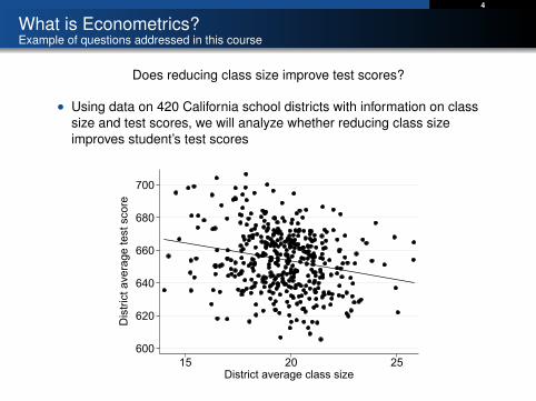
What is Econometrics?Example of questions addressed in this course
Does reducing class size improve test scores?
• Using data on 420 California school districts with information on classsize and test scores, we will analyze whether reducing class sizeimproves student’s test scores
600
620
640
660
680
700
Dis
trict
ave
rage
test
sco
re
15 20 25District average class size

5
What is Econometrics?Example of questions addressed in this course
What are the returns to education?
• Using data on 3,010 full-time working men in the US we will analyzewhether obtaining more years of education increase wages.
4
5
6
7
8
ln(w
age)
0 5 10 15 20years of education
6
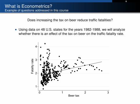
What is Econometrics?Example of questions addressed in this course
Does increasing the tax on beer reduce traffic fatalities?
• Using data on 48 U.S. states for the years 1982-1988, we will analyzewhether there is an effect of the tax on beer on the traffic fatality rate.
1
2
3
4
Fata
lity
rate
0 1 2 3Beer tax

7
Course outline
15 Lectures; 10 Seminars; 3 Stata seminars
Course Material:
• James Stock and Mark. M. Watson, Introduction to Econometrics (3rdedition update), Pearson, 2015.
• Chapter 1-12, 13.1-13.5 and 13.7, 14.1-14.6 and 14.8.• Lecture slides
Exam:
• Written examination on 25 May at 02:30 (3 hours)• Open book examination where all printed and written resources, in
addition to calculator, are allowed.
Term paper:
• Term paper will be an empirical project, handed out on 29 January 2018.• Not possible to take the written school exam if the compulsory term
paper is not approved.
8
Learning outcomes
At the end of this course you should
• have knowledge of regression analysis relevant for analyzing economicdata.
• be able to interpret and critically evaluate outcomes of an empiricalanalysis
• know the theoretical background and assumptions for standardeconometric methods
• be able to use Stata to perform an empirical analyses
• be able to read and understand journal articles that make use of themethods introduced in this course
• be able to make use of econometric models in your own academic work,for example in your master’s thesis

9
Course outline
Lecture 1: Introduction and Review of Statistics (S&W Ch 1-2)
Lecture 2: Review of Statistics (S&W Ch 2-3)
Lecture 3: Review of Statistics & Ordinary Least Squares (S&W Ch 3-4)
Lecture 4: Linear regression with one regressor (S&W Ch 4)
Lecture 5: Hypothesis tests & confidence intervals–One regressor (S&W Ch 5)
Lecture 6: Linear regression with multiple regressors (S&W Ch 6)
Lecture 7: Hypothesis tests & conf. intervals–Multiple regressors (S&W Ch 7)
Lecture 8: Nonlinear regression (S&W Ch 8)
Lecture 9: Internal and external validity (S&W Ch 9)
Lecture 10: Panel data (S&W Ch 10)
Lecture 11: Binary dependent variables (S&W Ch 11)
Lecture 12: Instrumental variable approach (S&W Ch 12)
Lecture 13: Experiments (S&W Ch 12-13)
Lecture 14: Quasi experiments (S&W Ch 13)
Lecture 15: Introduction to time series analysis (S&W Ch 14)

Review of Statistics
11
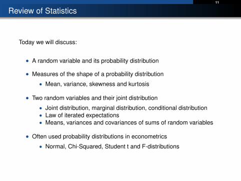
Review of Statistics
Today we will discuss:
• A random variable and its probability distribution
• Measures of the shape of a probability distribution
• Mean, variance, skewness and kurtosis
• Two random variables and their joint distribution
• Joint distribution, marginal distribution, conditional distribution• Law of iterated expectations• Means, variances and covariances of sums of random variables
• Often used probability distributions in econometrics
• Normal, Chi-Squared, Student t and F-distributions
12
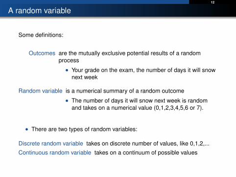
A random variable
Some definitions:
Outcomes are the mutually exclusive potential results of a randomprocess
• Your grade on the exam, the number of days it will snownext week
Random variable is a numerical summary of a random outcome
• The number of days it will snow next week is randomand takes on a numerical value (0,1,2,3,4,5,6 or 7).
• There are two types of random variables:
Discrete random variable takes on discrete number of values, like 0,1,2,...
Continuous random variable takes on a continuum of possible values
13
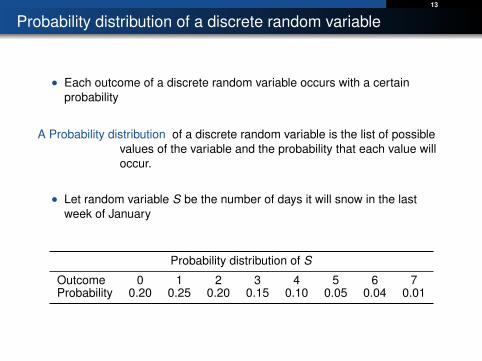
Probability distribution of a discrete random variable
• Each outcome of a discrete random variable occurs with a certainprobability
A Probability distribution of a discrete random variable is the list of possiblevalues of the variable and the probability that each value willoccur.
• Let random variable S be the number of days it will snow in the lastweek of January
Probability distribution of S
Outcome 0 1 2 3 4 5 6 7Probability 0.20 0.25 0.20 0.15 0.10 0.05 0.04 0.01

14
Cumulative distribution of a discrete random variable
A cumulative probability distribution is the probability that the randomvariable is less than or equal to a particular value
• The probability that it will snow less than or equal to s days,F (s) = Pr(S ≤ s) is the cumulative probability distribution of Sevaluated at s
• A cumulative probability distribution is also referred to as a cumulativedistribution or a CDF.
(cumulative) Probability distribution of S
Outcome 0 1 2 3 4 5 6 7Probability 0.20 0.25 0.20 0.15 0.10 0.05 0.04 0.01CDF 0.20 0.45 0.65 0.80 0.90 0.95 0.99 1

15
Probability distribution of a continuous random variable
• Tomorrow’s temperature is an example of a continuous random variable
• The CDF is defined similar to a discrete random variable.
• A probability distribution that lists all values and the probability of eachvalue is not suitable for a continuous random variable.
• Instead the probability is summarized in a probability density function(PDF/ density)
Area to the left of the redline: Pr(T <= -5) = 0.5
0
.02
.04
.06
.08
Pro
babi
lity
dens
ity
-30 -20 -10 0 10Tomorrow's temperature
0
.2
.4
.6
.8
1
Cum
ulat
ive
dist
ribut
ion
func
tion
-30 -20 -10 0 10 20Tomorrow's temperature

16
Measures of the shape of a probability distributionExpected value
The expected value or mean of a random variable is the average value overmany repeated trails or occurrences.
Suppose a discrete random value Y takes on k possible values
E (Y ) =k∑
i=1
yi · Pr(Y = yi ) = µY
Number of days it will snow in the last week of January (S)
Outcome 0 1 2 3 4 5 6 7Probability 0.20 0.25 0.20 0.15 0.10 0.05 0.04 0.01
E (S) = 0·0.2+1·0.25+2·0.2+3·0.15+4·0.1+5·0.05+6·0.04+7·0.01 = 2.06
Expected value of a continuous random variable
E (Y ) =
∫ ∞−∞
y · f (y)dy = µY
17
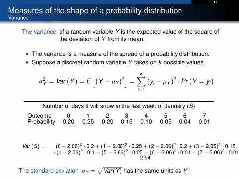
Measures of the shape of a probability distributionVariance
The variance of a random variable Y is the expected value of the square ofthe deviation of Y from its mean.
• The variance is a measure of the spread of a probability distribution.• Suppose a discreet random variable Y takes on k possible values
σ2Y = Var (Y ) = E
[(Y − µY )
2]=
k∑i=1
(yi − µY )2 · Pr (Y = yi)
Number of days it will snow in the last week of January (S)
Outcome 0 1 2 3 4 5 6 7Probability 0.20 0.25 0.20 0.15 0.10 0.05 0.04 0.01
Var (S) = (0 − 2.06)2 · 0.2 + (1 − 2.06)2 · 0.25 + (2 − 2.06)2 · 0.2 + (3 − 2.06)2 · 0.15+(4 − 2.06)2 · 0.1 + (5 − 2.06)2 · 0.05 + (6 − 2.06)2 · 0.04 + (7 − 2.06)2 · 0.01
2.94
The standard deviation σY =√
Var(Y ) has the same units as Y
18
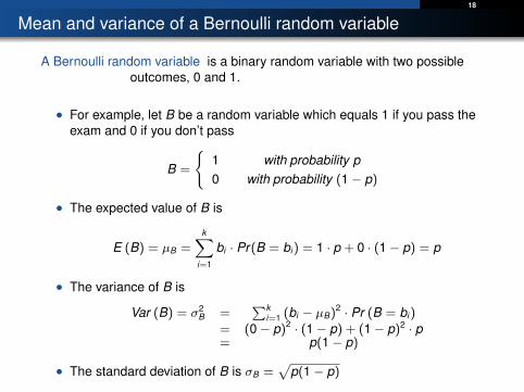
Mean and variance of a Bernoulli random variable
A Bernoulli random variable is a binary random variable with two possibleoutcomes, 0 and 1.
• For example, let B be a random variable which equals 1 if you pass theexam and 0 if you don’t pass
B =
{10
with probability pwith probability (1− p)
• The expected value of B is
E (B) = µB =k∑
i=1
bi · Pr(B = bi ) = 1 · p + 0 · (1− p) = p
• The variance of B is
Var (B) = σ2B =
∑ki=1 (bi − µB)2 · Pr (B = bi )
= (0− p)2 · (1− p) + (1− p)2 · p= p(1− p)
• The standard deviation of B is σB =√
p(1− p)

19
Mean and variance of a linear function of a random variable
• In this course we will consider random variables (say X and Y ) that arerelated by a linear function
Y = a + b · X
• Suppose E (X ) = µX and Var (X ) = σ2X
• This implies that the expected value of Y equals
E (Y ) = µY = E (a + b · X ) = a + b · E (X ) = a + b · µX
• The variance of Y equals
Var (Y ) = σ2Y = E
[(Y − µY )2
]= E
[((a + bX )− (a + bµX ))2
]= E
[b2(X − µX )2]
= b2E[(X − µX )2]
= b2 · σ2X

20
Measures of the shape of a probability distribution: Skewness
Skewness is a measure of the lack of symmetry of a distribution
Skewness =E[(Y − µY )3
]σ3
Y
Positive SkewNegative Skew
• For a symmetric distribution positive values of (Y − µY )3are offset bynegative values (equally likely) and skewness is 0
• For a negatively (positively) skewed distribution negative (positive)values of (Y − µY )3 are more likely and the skewness is negative(positive).
• Skewness is unit free.
21
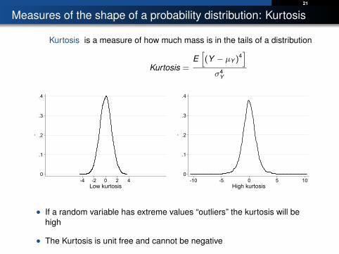
Measures of the shape of a probability distribution: Kurtosis
Kurtosis is a measure of how much mass is in the tails of a distribution
Kurtosis =E[(Y − µY )4
]σ4
Y
0
.1
.2
.3
.4
.
-4 -2 0 2 4Low kurtosis
0
.1
.2
.3
.4
.-10 -5 0 5 10
High kurtosis
• If a random variable has extreme values “outliers” the kurtosis will behigh
• The Kurtosis is unit free and cannot be negative

22
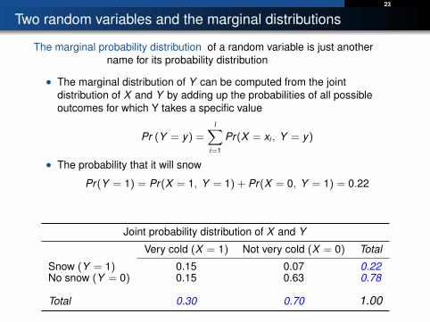
Two random variables and their joint distribution
• Most of the interesting questions in economics involve 2 or more randomvariables
• Answering these questions requires understanding the concepts of joint,marginal and conditional probability distribution.
The joint probability distribution of two random variables X and Y can bewritten as Pr(X = x , Y = y)
• Let Y equal 1 if it snows and 0 if it does not snow.• Let X equal 1 if it is very cold and 0 if it is not very cold.
Joint probability distribution of X and Y
Very cold (X = 1) Not very cold (X = 0) Total
Snow (Y = 1) 0.15 0.07 0.22No snow (Y = 0) 0.15 0.63 0.78
Total 0.30 0.70 1.00
23
Two random variables and the marginal distributions
The marginal probability distribution of a random variable is just anothername for its probability distribution
• The marginal distribution of Y can be computed from the jointdistribution of X and Y by adding up the probabilities of all possibleoutcomes for which Y takes a specific value
Pr (Y = y) =l∑
i=1
Pr(X = xi , Y = y)
• The probability that it will snow
Pr(Y = 1) = Pr(X = 1, Y = 1) + Pr(X = 0, Y = 1) = 0.22
Joint probability distribution of X and Y
Very cold (X = 1) Not very cold (X = 0) Total
Snow (Y = 1) 0.15 0.07 0.22No snow (Y = 0) 0.15 0.63 0.78
Total 0.30 0.70 1.00
24
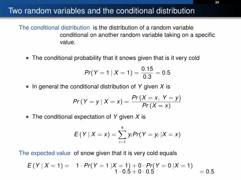
Two random variables and the conditional distribution
The conditional distribution is the distribution of a random variableconditional on another random variable taking on a specificvalue.
• The conditional probability that it snows given that is it very cold
Pr(Y = 1 | X = 1) =0.150.3
= 0.5
• In general the conditional distribution of Y given X is
Pr (Y = y | X = x) =Pr (X = x , Y = y)
Pr (X = x)
• The conditional expectation of Y given X is
E (Y | X = x) =k∑
i=1
yiPr(Y = yi |X = x)
The expected value of snow given that it is very cold equals
E (Y | X = 1) = 1 · Pr(Y = 1 |X = 1) + 0 · Pr(Y = 0 |X = 1)1 · 0.5 + 0 · 0.5 = 0.5
25
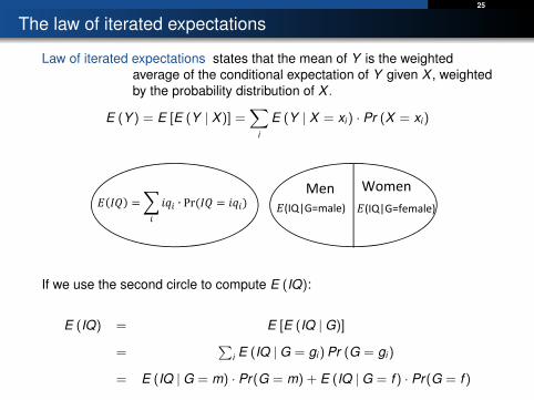
The law of iterated expectations
Law of iterated expectations states that the mean of Y is the weightedaverage of the conditional expectation of Y given X , weightedby the probability distribution of X .
E (Y ) = E [E (Y | X )] =∑
i
E (Y | X = xi ) · Pr (X = xi )
∙ Pr (IQ|G=female) (IQ|G=male)
Women Men
If we use the second circle to compute E (IQ):
E (IQ) = E [E (IQ |G)]
=∑
i E (IQ |G = gi ) Pr (G = gi )
= E (IQ |G = m) · Pr(G = m) + E (IQ |G = f ) · Pr(G = f )

26
Independence
Independence: Two random variables X and Y are independent if theconditional distribution of Y given X does not depend on X
Pr (Y = y | X = x) = Pr (Y = y)
• If X and Y are independent this also implies
Pr (X = x , Y = y) = Pr (X = x) · Pr (Y = y |X = x)(see slide 23)
= Pr (X = x) · Pr (Y = y)
Mean independence: The conditional mean of Y given X equals theunconditional mean of Y
E (Y | X ) = E (Y )
• For example if the expected value of snow (Y ) does not depend onwhether it is very cold (X )
E (Y | X = 1) = E (Y | X = 0) = E (Y )
27
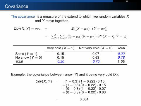
Covariance
The covariance is a measure of the extend to which two random variables Xand Y move together,
Cov(X ,Y ) = σXY = E [(X − µX ) · (Y − µY )]
=∑k
i=1
∑lj=1(xj − µX )(yi − µY ) · Pr (X = xj ,Y = yi )
Very cold (X = 1) Not very cold (X = 0) Total
Snow (Y = 1) 0.15 0.07 0.22No snow (Y = 0) 0.15 0.63 0.78Total 0.30 0.70 1.00
Example: the covariance between snow (Y) and it being very cold (X):
Cov(X ,Y ) = (1− 0.3) (1− 0.22) · 0.15+ (1− 0.3) (0− 0.22) · 0.15+ (0− 0.3) (1− 0.22) · 0.07+ (0− 0.3) (0− 0.22) · 0.63
= 0.084
28
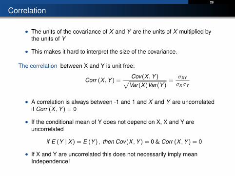
Correlation
• The units of the covariance of X and Y are the units of X multiplied bythe units of Y
• This makes it hard to interpret the size of the covariance.
The correlation between X and Y is unit free:
Corr (X ,Y ) =Cov(X ,Y )√
Var(X )Var(Y )=
σXY
σXσY
• A correlation is always between -1 and 1 and X and Y are uncorrelatedif Corr (X ,Y ) = 0
• If the conditional mean of Y does not depend on X, X and Y areuncorrelated
if E (Y | X ) = E (Y ) , then Cov(X ,Y ) = 0 & Corr (X ,Y ) = 0
• If X and Y are uncorrelated this does not necessarily imply meanIndependence!
29
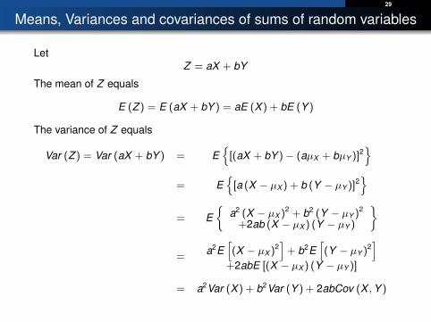
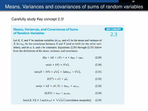
Means, Variances and covariances of sums of random variables
LetZ = aX + bY
The mean of Z equals
E (Z ) = E (aX + bY ) = aE (X ) + bE (Y )
The variance of Z equals
Var (Z ) = Var (aX + bY ) = E{
[(aX + bY )− (aµX + bµY )]2}
= E{
[a (X − µX ) + b (Y − µY )]2}
= E{
a2 (X − µX )2 + b2 (Y − µY )2
+2ab (X − µX ) (Y − µY )
}
=a2E
[(X − µX )2
]+ b2E
[(Y − µY )2
]+2abE [(X − µX ) (Y − µY )]
= a2Var (X ) + b2Var (Y ) + 2abCov (X ,Y )
30
Means, Variances and covariances of sums of random variables
Carefully study Key concept 2.3!
PRINTED BY: [email protected]. Printing is for personal, private use only. No part of this book may be reproduced or transmitted without publisher's prior permission. Violators will be prosecuted.
Page 1 of 1Introduction to Econometrics, Update, Global Edtion
06.01.2017https://jigsaw.vitalsource.com/api/v0/books/9781292071367/print?from=81&to=81
Examples of often used probability distributions inEconometrics

32
The Normal distribution
The most often encountered probability density function in econometrics isthe Normal distribution:
fY (y) =1
σ√
2πexp
[−1
2
(y − µσ
)]• A normal distribution with mean µ and standard deviation σ is denoted
as N (µ, σ)
.
µ-1.96*σ µ µ-1.96*σ.
33
The Normal distribution
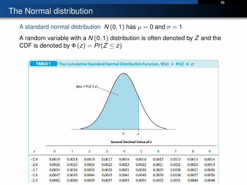
A standard normal distribution N (0, 1) has µ = 0 and σ = 1
A random variable with a N (0, 1) distribution is often denoted by Z and theCDF is denoted by Φ (z) = Pr(Z ≤ z)
PRINTED BY: [email protected]. Printing is for personal, private use only. No part of this book may be reproduced or transmitted without publisher's prior permission. Violators will be prosecuted.
Page 1 of 1Introduction to Econometrics, Update, Global Edtion
06.01.2017https://jigsaw.vitalsource.com/api/v0/books/9781292071367/print?from=803&to=803
34
The Normal distribution
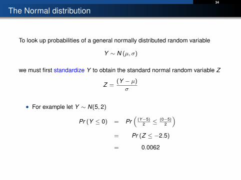
To look up probabilities of a general normally distributed random variable
Y ∼ N (µ, σ)
we must first standardize Y to obtain the standard normal random variable Z
Z =(Y − µ)
σ
• For example let Y ∼ N(5, 2)
Pr (Y ≤ 0) = Pr(
(Y−5)2 ≤ (0−5)
2
)= Pr (Z ≤ −2.5)
= 0.0062
35
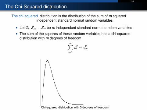
The Chi-Squared distribution
The chi-squared distribution is the distribution of the sum of m squaredindependent standard normal random variables
• Let Z1,Z2, ...,Zm be m independent standard normal random variables
• The sum of the squares of these random variables has a chi-squareddistribution with m degrees of freedom
m∑i=1
Z 2i ∼ χ2
m
.
Chi-squared distribution with 5 degrees of freedom

36
The Chi-Squared distribution
• The chi-squared distribution is used when testing hypotheses ineconometrics
• Appendix table 3 shows the 90th 95th and 99th percentiles of theχ2-distribution
• For example Pr(∑3
i=1 Z 2i ≤ 7.81
)= 0.95
PRINTED BY: [email protected]. Printing is for personal, private use only. No part of this book may be reproduced or transmitted without publisher's prior permission. Violators will be prosecuted.
Page 1 of 1Introduction to Econometrics, Update, Global Edtion
06.01.2017https://jigsaw.vitalsource.com/api/v0/books/9781292071367/print?from=806&to=806

37
The Student t distribution
Let Z be a standard normal random variable and W a Chi-Squareddistributed random variable with m degrees of freedom
The Student t-distribution with m degrees of freedom is the distribution therandom variable Z√
W/m
2.5% 2.5%95%
.
-2.57 2.57Student t distribution with 5 degrees of freedom
• The t distribution has fatter tails than the standard normal distribution.
• When m ≥ 30 it is well approximated by the standard normaldistribution.

38
The Student t distribution
• The Student t distribution is often used when testing hypotheses ineconometrics
• Appendix Table 2 shows selected percentiles of the tm distribution
• For example with m = 5;
Pr (t < −2.57) = 0.025; Pr (|t | > 2.57) = 0.05; Pr (t > 2.57) = 0.025PRINTED BY: [email protected]. Printing is for personal, private use only. No part of this book may be reproduced or transmitted without publisher's prior permission. Violators will be prosecuted.
Page 1 of 1Introduction to Econometrics, Update, Global Edtion
06.01.2017https://jigsaw.vitalsource.com/api/v0/books/9781292071367/print?from=805&to=805
39
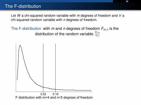
The F-distribution
Let W a chi-squared random variable with m degrees of freedom and V achi-squared random variable with n degrees of freedom.
The F-distribution with m and n degrees of freedom Fm,n is thedistribution of the random variable
W/mV/n
.
3.52 5.19F distribution with m=4 and n=5 degrees of freedom
40
The F-distribution
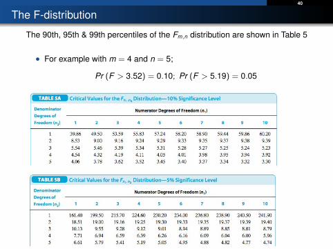
The 90th, 95th & 99th percentiles of the Fm,n distribution are shown in Table 5
• For example with m = 4 and n = 5;
Pr (F > 3.52) = 0.10; Pr (F > 5.19) = 0.05
PRINTED BY: [email protected]. Printing is for personal, private use only. No part of this book may be reproduced or transmitted without publisher's prior permission. Violators will be prosecuted.
Page 1 of 1Introduction to Econometrics, Update, Global Edtion
09.01.2017https://jigsaw.vitalsource.com/api/v0/books/9781292071367/print?from=808&to=808
PRINTED BY: [email protected]. Printing is for personal, private use only. No part of this book may be reproduced or transmitted without publisher's prior permission. Violators will be prosecuted.
Page 1 of 1Introduction to Econometrics, Update, Global Edtion
09.01.2017https://jigsaw.vitalsource.com/api/v0/books/9781292071367/print?from=809&to=809

41
The F-distribution
• A special case of the F distribution which is often used in econometricsis when Fm,n can be approximated by Fm,∞
• In this limiting case the denominator is the mean of infinitely manysquared standard normal random variables, which equals 1.
• Appendix Table 4 shows the 90th, 95th and 99th percentiles of the Fm,∞distribution.
PRINTED BY: [email protected]. Printing is for personal, private use only. No part of this book may be reproduced or transmitted without publisher's prior permission. Violators will be prosecuted.
Page 1 of 1Introduction to Econometrics, Update, Global Edtion
09.01.2017https://jigsaw.vitalsource.com/api/v0/books/9781292071367/print?from=807&to=807
Top Related