�

� �

�

�

� �

�

PROCESS MODELINGAND SIMULATION FORCHEMICAL ENGINEERS

�

� �

�

�

� �

�

PROCESS MODELINGAND SIMULATION FORCHEMICAL ENGINEERSTHEORY AND PRACTICE

Simant Ranjan Upreti

Department of Chemical Engineering,Ryerson University,Toronto, Canada

�

� �

�

This edition first published 2017© 2017 John Wiley & Sons Ltd

All rights reserved. No part of this publication may be reproduced, stored in a retrieval system, or transmitted, in anyform or by any means, electronic, mechanical, photocopying, recording or otherwise, except as permitted by law.Advice on how to obtain permision to reuse material from this title is available athttp://www.wiley.com/go/permissions.

The right of Simant Ranjan Upreti to be identified as the author of this work has been asserted in accordance withlaw.

Registered OfficesJohn Wiley & Sons, Inc., 111 River Street, Hoboken, NJ 07030, USAJohn Wiley & Sons Ltd, The Atrium, Southern Gate, Chichester, West Sussex, PO19 8SQ, UK

Editorial OfficeThe Atrium, Southern Gate, Chichester, West Sussex, PO19 8SQ, UK

For details of our global editorial offices, customer services, and more information about Wiley products visit us atwww.wiley.com.

Wiley also publishes its books in a variety of electronic formats and by print-on-demand. Some content that appearsin standard print versions of this book may not be available in other formats.

Limit of Liability/Disclaimer of WarrantyThe publisher and the authors make no representations or warranties with respect to the accuracy or completeness ofthe contents of this work and specifically disclaim all warranties, including without limitation any impliedwarranties of fitness for a particular purpose. This work is sold with the understanding that the publisher is notengaged in rendering professional services. The advice and strategies contained herein may not be suitable for everysituation. In view of ongoing research, equipment modifications, changes in governmental regulations, and theconstant flow of information relating to the use of experimental reagents, equipment, and devices, the reader is urgedto review and evaluate the information provided in the package insert or instructions for each chemical, piece ofequipment, reagent, or device for, among other things, any changes in the instructions or indication of usage and foradded warnings and precautions. The fact that an organization or website is referred to in this work as a citationand/or potential source of further information does not mean that the author or the publisher endorses theinformation the organization or website may provide or recommendations it may make. Further, readers should beaware that websites listed in this work may have changed or disappeared between when this works was written andwhen it is read. No warranty may be created or extended by any promotional statements for this work. Neither thepublisher nor the author shall be liable for any damages arising herefrom.

Library of Congress Cataloging-in-Publication Data

Names: Upreti, Simant Ranjan, author.Title: Process modeling and simulation for chemical engineers : theory andpractice / Simant Ranjan Upreti.

Description: Chichester, UK ; Hoboken, NJ : John Wiley & Sons, 2017. |Includes bibliographical references and index.

Identifiers: LCCN 2016053339| ISBN 9781118914687 (cloth) | ISBN 9781118914663(epub)

Subjects: LCSH: Chemical processes–Mathematical models. | Chemicalprocesses–Data processing.

Classification: LCC TP155.7 .U67 2017 | DDC 660/.284401–dc23LC record available at https://lccn.loc.gov/2016053339

Cover image: shulz/GettyimagesCover design by Wiley

Set in 10/12pt, NimbusRomNo by SPi Global, Chennai, India.

10 9 8 7 6 5 4 3 2 1

�

� �

�

to my wife and kids

�

� �

�

CONTENTS

Preface xiii

Notation xv

1 Introduction 1

1.1 System 11.1.1 Uniform System 21.1.2 Properties of System 21.1.3 Classification of System 31.1.4 Model 3

1.2 Process 31.2.1 Classification of Processes 41.2.2 Process Model 5

1.3 Process Modeling 61.3.1 Relations 71.3.2 Assumptions 71.3.3 Variables and Parameters 8

1.4 Process Simulation 91.4.1 Utility 91.4.2 Simulation Methods 10

1.5 Development of Process Model 11

1.6 Learning about Process 13

1.7 System Specification 14

Bibliography 16

Exercises 16

2 Fundamental Relations 17

2.1 Basic Form 172.1.1 Application 19

2.2 Mass Balance 21

viii

2.2.1 Microscopic Balances 212.2.2 Equation of Change for Mass Fraction 23

2.3 Mole Balance 242.3.1 Microscopic Balances 242.3.2 Equation of Change for Mole Fraction 25

2.4 Momentum Balance 262.4.1 Convective Momentum Flux 272.4.2 Total Momentum Flux 282.4.3 Macroscopic Balance 292.4.4 Microscopic Balance 31

2.5 Energy Balance 332.5.1 Microscopic Balance 332.5.2 Macroscopic Balance 35

2.6 Equation of Change for Kinetic and Potential Energy 382.6.1 Microscopic Equation 382.6.2 Macroscopic Equation 40

2.7 Equation of Change for Temperature 412.7.1 Microscopic Equation 412.7.2 Macroscopic Equation 42

2.A Enthalpy Change from Thermodynamics 44

2.B Divergence Theorem 48

2.C General Transport Theorem 50

2.D Equations in Cartesian, Cylindrical and Spherical Coordinate Systems 532.D.1 Equations of Continuity 542.D.2 Equations of Continuity for Individual Species 542.D.3 Equations of Motion 552.D.4 Equations of Change for Temperature 56

Bibliography 57

Exercises 57

3 Constitutive Relations 59

3.1 Diffusion 593.1.1 Multicomponent Mixtures 60

3.2 Viscous Motion 603.2.1 Newtonian Fluids 613.2.2 Non-Newtonian Fluids 62

3.3 Thermal Conduction 63

3.4 Chemical Reaction 63

3.5 Rate of Reaction 65

ix

3.5.1 Equations of Change for Moles 663.5.2 Equations of Change for Temperature 673.5.3 Macroscopic Equation of Change for Temperature 69

3.6 Interphase Transfer 71

3.7 Thermodynamic Relations 72

3.A Equations in Cartesian, Cylindrical and Spherical Coordinate Systems 743.A.1 Equations of Continuity for Binary Systems 743.A.2 Equations of Motion for Newtonian Fluids 753.A.3 Equations of Change for Temperature 76

References 77

Bibliography 77

Exercises 78

4 Model Formulation 79

4.1 Lumped-Parameter Systems 804.1.1 Isothermal CSTR 804.1.2 Flow through Eccentric Reducer 834.1.3 Liquid Preheater 844.1.4 Non-Isothermal CSTR 87

4.2 Distributed-Parameter Systems 904.2.1 Nicotine Patch 904.2.2 Fluid Flow between Inclined Parallel Plates 934.2.3 Tapered Fin 964.2.4 Continuous Microchannel Reactor 994.2.5 Oxygen Transport to Tissues 1034.2.6 Dermal Heat Transfer in Cylindrical Limb 1064.2.7 Solvent Induced Heavy Oil Recovery 1084.2.8 Hydrogel Tablet 1124.2.9 Neutron Diffusion 1174.2.10 Horton Sphere 1194.2.11 Reactions around Solid Reactant 122

4.3 Fluxes along Non-Linear Directions 1274.3.1 Saccadic Movement of an Eye 128

4.A Initial and Boundary Conditions 1314.A.1 Initial Condition 1314.A.2 Boundary Condition 1314.A.3 Periodic Condition 132

4.B Zero Derivative at the Point of Symmetry 133

4.C Equation of Motion along the Radial Direction in Cylindrical Coordinates 134

References 137

x

Exercises 137

5 Model Transformation 139

5.1 Transformation between Orthogonal Coordinate Systems 1395.1.1 Scale Factors 1395.1.2 Differential Elements 1425.1.3 Vector Representation 1435.1.4 Derivatives of Unit Vectors 1445.1.5 Differential Operators 146

5.2 Transformation between Arbitrary Coordinate Systems 1555.2.1 Transformation of Velocity 1555.2.2 Transformation of Spatial Derivatives 1565.2.3 Correctness of Transformation Matrices 156

5.3 Laplace Transformation 1615.3.1 Examples 1625.3.2 Properties of Laplace Transforms 1645.3.3 Solution of Linear Differential Equations 168

5.4 Miscellaneous Transformations 1785.4.1 Higher Order Derivatives 1785.4.2 Scaling 1785.4.3 Change of Independent Variable 1795.4.4 Semi-Infinite Domain 1795.4.5 Non-Autonomous to Autonomous Differential Equation 180

5.A Differential Operators in an Orthogonal Coordinate System 1805.A.1 Gradient of a Scalar 1805.A.2 Divergence of a Vector 1815.A.3 Laplacian of a Scalar 1845.A.4 Curl of a Vector 184

References 186

Bibliography 186

Exercises 186

6 Model Simplification and Approximation 189

6.1 Model Simplification 1896.1.1 Scaling and Ordering Analysis 1906.1.2 Linearization 193

6.2 Model Approximation 2006.2.1 Dimensional Analysis 2016.2.2 Model Fitting 204

6.A Linear Function 220

6.B Proof of Buckingham Pi Theorem 221

xi

6.C Newton’s Optimization Method 223

References 224

Bibliography 224

Exercises 225

7 Process Simulation 227

7.1 Algebraic Equations 2277.1.1 Linear Algebraic Equations 2277.1.2 Non-Linear Algebraic Equations 236

7.2 Differential Equations 2417.2.1 Ordinary Differential Equations 2427.2.2 Explicit Runge–Kutta Methods 2427.2.3 Step-Size Control 2467.2.4 Stiff Equations 247

7.3 Partial Differential Equations 2537.3.1 Finite Difference Method 255

7.4 Differential Equations with Split Boundaries 2637.4.1 Shooting Newton–Raphson Method 264

7.5 Periodic Differential Equations 2687.5.1 Shooting Newton–Raphson Method 268

7.6 Programming of Derivatives 271

7.7 Miscellanea 2747.7.1 Integration of Discrete Data 2747.7.2 Roots of a Single Algebraic Equation 2767.7.3 Cubic Equations 278

7.A Partial Pivoting for Matrix Inverse 281

7.B Derivation of Newton–Raphson Method 2817.B.1 Quadratic Convergence 282

7.C General Derivation of Finite Difference Formulas 2847.C.1 First Derivative, Centered Second Order Formula 2857.C.2 Second Derivative, Forward Second Order Formula 2867.C.3 Third Derivative, Mixed Fourth Order Formula 2877.C.4 Common Finite Difference Formulas 289

References 291

Bibliography 291

Exercises 291

8 Mathematical Review 295

8.1 Order of Magnitude 295

xii

8.2 Big-O Notation 295

8.3 Analytical Function 295

8.4 Vectors 2968.4.1 Vector Operations 2978.4.2 Cauchy–Schwarz Inequality 302

8.5 Matrices 3028.5.1 Terminology 3038.5.2 Matrix Operations 3048.5.3 Operator Inequality 305

8.6 Tensors 3068.6.1 Multilinearity 3068.6.2 Coordinate-Independence 3068.6.3 Representation of Second Order Tensor 3078.6.4 Einstein or Index Notation 3088.6.5 Kronecker Delta 3108.6.6 Operations Involving Vectors and Second Order Tensors 310

8.7 Differential 3188.7.1 Derivative 3188.7.2 Partial Derivative and Differential 3188.7.3 Chain Rule of Differentiation 3198.7.4 Material and Total Derivatives 321

8.8 Taylor Series 3228.8.1 Multivariable Taylor Series 3238.8.2 First Order Taylor Expansion 323

8.9 L’Hopital’s Rule 326

8.10 Leibniz’s Rule 326

8.11 Integration by Parts 327

8.12 Euler’s Formulas 327

8.13 Solution of Linear Ordinary Differential Equations 3278.13.1 Single First Order Equation 3278.13.2 Simultaneous First Order Equations 328

Bibliography 332

Index 333

PREFACE

I am delighted to present this book on process modeling and simulation for chemicalengineers. It is a humble attempt to assimilate the amazing contributions of researchers andacademicians in this area.

The goal of this book is to provide a rigorous treatment of fundamental concepts andtechniques of this subject. To that end, the book includes all requisite mathematical analysesand derivations, which could be sometimes hard to find. Target readers are those at thegraduate level. This book endeavors to equip them to model sophisticated processes, developrequisite computational algorithms and programs, improvise existing software, and solveresearch problems with confidence.

Chapter 1 provides the groundwork by introducing the terminology of process modelingand simulation. Chapter 2 presents the fundamental relations for this subject. Chapter 3incorporates important constitutive relations for common systems. Chapter 4 presents modelformulation with the help of several examples. Transformation techniques are introducedin Chapter 5. Model simplification and approximation methods are discussed in Chapter 6.The numerical solution of process models is the theme of Chapter 7. Review of importantmathematical concepts is provided in Chapter 8.

This book can be used as a primary text for a one-semester course. Alternatively, it could serve as a supplementary text in graduate courses related to modeling and simulation. Readers could also study the book on their own. During an initial reading, one could very well skim quickly through a derivation, accept the result for the time being, and learn more from applications. Computer programs for the solutions of book examples can be obtained from the publisher’s website,www.wiley.com/go/upreti/pms for chemical engineers.

I am grateful to the editorial team at John Wiley & Sons for providing excellent supportfrom start to finish.

Finally, I am deeply indebted to my wife Deepa, and children Jahnavi and Pranav. I couldnot have completed this book without their unsparing support and understanding.

Ryerson University, Toronto Simant R. Upreti

Notation

Symbol Description Units

a surface area per unit volume m−1

Am area of moving surfaces m2

Ap area of a port of flow m2

A area m2

A area vector m2

c average concentration of a mixture kmolm−3

ci concentration of the ith species kmolm−3

CP specific heat capacity of mixture J kg−1K−1

CPi CP of the ith species in pure form J kg−1K−1

¯CP,i molar specific heat capacity of the ith species in a

mixtureJ kmol−1K−1

CP,i partial specific heat capacity of the ith species in amixture

J kmol−1K−1

dx differential change in x of x

D diffusivity of species m2 s−1

DAB binary diffusivity of A in a mixture of A and B m2 s−1

D matrix of multicomponent diffusivities m2 s−1

ei the ith component of energy flux Jm−2 s−1

E sum of the squared errors in y in a population of y2

E total energy of a system J

E activation energy of reaction J kmol−1

E energy per unit mass J kg−1

fi fugacity of the ith species Pa

F volumetric flow rate m3 s−1

fi mass flux of the ith species kgm−2 s−1

f overall mass flux of a mixture kgm−2 s−1

xvi

Symbol Description Units

Fi molar flux of the ith species kmolm−2 s−1

F overall molar flux of a mixture kmolm−2 s−1

F force vector N

G Gibbs free energy J

Gi Gibbs free energy per unit mass of the ith species J kg−1

g gravity, 9.806 65 m s−2

h heat transfer coefficient Wm−2 K−1

H enthalpy J

H enthalpy per unit mass J kg−1

Hi Henry’s law constant for the ith species Pa

Hi enthalpy per unit mass of the ith species J kg−1

Hi partial specific enthalpy of the ith species in amixture

J kg−1

Hi partial molar enthalpy of the ith species in a mixture J kmol−1

¯Hi molar enthalpy of the ith species in pure form J kmol−1

¯H◦

i standard¯Hi J kmol−1

H Hessian matrix

I identity matrix

ji diffusive mass flux of the ith species kgm−2 s−1

j vector of ji kgm−2 s−1

J Jacobian matrixJi diffusive molar flux of the ith species kmolm−2 s−1

J vector of Ji kmolm−2 s−1

k reaction rate coefficient as per reaction

k thermal conductivity Wm−1 K−1

k0 frequency factor as per reaction

kc mass transfer coefficient ms−1

K equilibrium constant of a chemical reaction

L lower triangular matrix

m mass kg

mi mass of the ith species kg

Mi molecular weight of the ith species kg kmol−1

Nc number of components or species

xvii

Symbol Description Units

Ni number of moles of the ith speciesNr number of chemical reactions

n, n,˜n unit vectors

pi partial pressure of the ith species Pa

P pressure Pa

Pc critical pressure Pa

p momentum kgm s−1

q rate of heat transfer J s−1

qi the ith component of conductive heat flux Jm−2 s−1

Q heat, i.e., energy in transit J

q conductive heat flux Jm−2 s−1

r correlation coefficientr rate of reaction kg(kmol)m−3 s−1

r radial direction in cylindrical and sphericalcoordinates

m

r2 coefficient of determinationR universal gas constant, 8.314 46× 103 J kmol−1 K−1

rgen,i mass rate of ith species generated per unit volume kgm−3 s−1

Rgen,i molar rate of ith species generated per unit volume kmolm−3 s−1

sy standard deviation in values of y of y

S entropy JK−1

Si entropy per unit mass of the ith species JK−1 kg−1

S sum of the squared errors from the average of y ina population

of y2

t time s

T temperature K, ◦CTc critical temperature ◦C

U internal energy J

U internal energy per unit mass J kg−1

Ui internal energy per unit mass of the ith species J kg−1

U upper triangular matrix

v magnitude of velocity ms−1

vi the ith component of v, or average velocity alongthe xi-direction

ms−1

xviii

Symbol Description Units

V volume m3

¯V molar volume m3 kmol−1

V specific volume m3 kg−1

Vi specific volume of the ith species m3 kg−1

v mass average velocity ms−1

v molar average velocity ms−1

Ws shaft work J

x change of x per unit time x -units s−1

xext amount of x from external source of x

xgen generated amount of x of x

X extent of chemical reactionX extent of chemical reaction per unit volume m−3

x� transpose of x (vector or matrix)xi unit vector along the xi-direction

‖x‖ norm or magnitude of x (vector or matrix)

z axial direction in cylindrical coordinates m

Greek Symbolsγ rate-of-strain tensor s−1

δij Kronecker deltaδQ net Q involved in differential changes, dU and dS J

δ unit dyadic (unit tensor)

ΔH◦i standard heat of formation of the ith species J kmol−1

ΔHr heat of reaction J kmol−1

ΔH◦r standard heat of reaction J kmol−1

Δx small amount of, or change in x of x

Δ[x] loss of x from a system through its ports of x

∇ gradient operator (a vector)

η Non-Newtonian viscosity Pa s

θ θ-direction in cylindrical and spherical coordinates rad, ◦

κ dilatational viscosity Pa s

μ viscosity Pa s

xix

Symbol Description Units

νi stoichiometric coefficient of ith species in achemical reaction

π molecular stress tensor Pa

Π dimensionless number

ρ density, mass concentration kgm−3

ρi density, mass concentration of the ith species kgm−3

τij , πij , φij the j th component of stress acting on the ith areacomponent

Pa

τ time period s

τ viscous stress tensor Pa

φ φ-direction in spherical coordinates rad, ◦

φ overall stress tensor Pa

Φ potential energy per unit mass J kg−1

ω mass fractionω acentric factorω vorticity tensor s−1

1Introduction

Process modeling and simulation is our intellectual endeavor to explain real-world processes,foresee their effects, and improve them to our satisfaction. Using foundational rules andthe language of mathematics, we describe a process, i.e., develop its model. Depending onwhat needs to be known, we pose the model as a problem. Its solution provides the neededinformation, thereby simulating the process as it would unfold in the real world.

This chapter lays the groundwork for process modeling and simulation. We explain thebasic concepts, and introduce the involved terminology in a methodical manner. Our startingpoint is the definition of a system.

1.1 SystemA system is defined as a set of one or more units relevant to the knowledge that is sought.Eventually, that knowledge is obtained as system characteristics, and their behavior in timeand space.

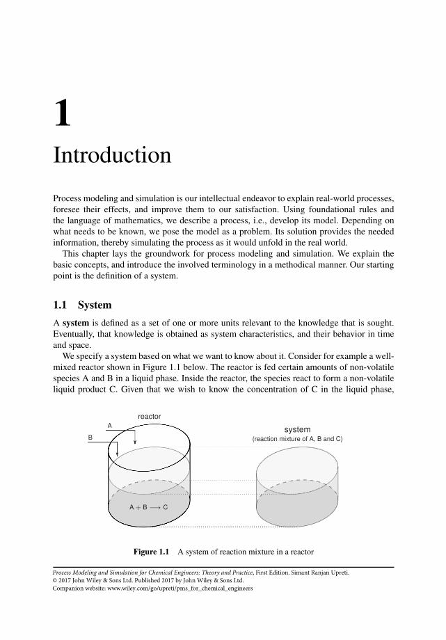
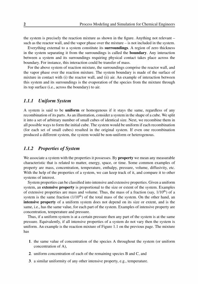
We specify a system based on what we want to know about it. Consider for example a well-mixed reactor shown in Figure 1.1 below. The reactor is fed certain amounts of non-volatilespecies A and B in a liquid phase. Inside the reactor, the species react to form a non-volatileliquid product C. Given that we wish to know the concentration of C in the liquid phase,

B

A system(reaction mixture of A, B and C)

A + B −→ C

reactor

Figure 1.1 A system of reaction mixture in a reactor

Process Modeling and Simulation for Chemical Engineers: Theory and Practice, First Edition. Simant Ranjan Upreti. © 2017 John Wiley & Sons Ltd. Published 2017 by John Wiley & Sons Ltd.Companion website: www.wiley.com/go/upreti/pms_for_chemical_engineers

2 Process Modeling and Simulation for Chemical Engineers

the system is precisely the reaction mixture as shown in the figure. Anything not relevant –such as the reactor wall, and the vapor phase over the mixture – is not included in the system.

Everything external to a system constitute its surroundings. A region of zero thicknessin the system separating it from the surroundings is called the boundary. Any interactionbetween a system and its surroundings requiring physical contact takes place across theboundary. For instance, this interaction could be transfer of mass.

For the above system of reaction mixture, the surroundings comprise the reactor wall, andthe vapor phase over the reaction mixture. The system boundary is made of the surface ofmixture in contact with (i) the reactor wall, and (ii) air. An example of interaction betweenthis system and its surroundings is the evaporation of the species from the mixture throughits top surface (i.e., across the boundary) to air.

1.1.1 Uniform System

A system is said to be uniform or homogenous if it stays the same, regardless of anyrecombination of its parts. As an illustration, consider a system in the shape of a cube. We splitit into a set of arbitrary number of small cubes of identical size. Next, we recombine them inall possible ways to form the initial cube. The system would be uniform if each recombination(for each set of small cubes) resulted in the original system. If even one recombinationproduced a different system, the system would be non-uniform or heterogenous.

1.1.2 Properties of System

We associate a system with the properties it possesses. By property we mean any measurablecharacteristic that is related to matter, energy, space, or time. Some common examples ofproperty are mass, concentration, temperature, enthalpy, pressure, volume, diffusivity, etc.With the help of the properties of a system, we can keep track of it, and compare it to othersystems of interest.

System properties can be classified into intensive and extensive properties. Given a uniformsystem, an extensive property is proportional to the size or extent of the system. Examplesof extensive properties are mass and volume. Thus, the mass of a fraction (say, 1/10th) of asystem is the same fraction (1/10th) of the total mass of the system. On the other hand, anintensive property of a uniform system does not depend on its size or extent, and is thesame, i.e., has the same value, for each part of the system. Examples of intensive property areconcentration, temperature and pressure.

Thus, if a uniform system is at a certain pressure then any part of the system is at the samepressure. Equivalently, if all intensive properties of a system do not vary then the system isuniform. An example is the reaction mixture of Figure 1.1 on the previous page. The mixturehas

1. the same value of concentration of the species A throughout the system (or uniformconcentration of A),

2. uniform concentration of each of the remaining species B and C, and

3. a similar uniformity of any other intensive property, e.g., temperature.

1. Introduction 3

For a non-uniform system, one or more intensive properties vary within the system. Moreprecisely, the properties vary with space inside the system. For example, if the reactionmixture of Figure 1.1 on p. 1 were not well-mixed then the species concentrations, andtemperature would not be the same throughout the mixture. In that situation, the mixturewould be a non-uniform system.

1.1.3 Classification of SystemBased on whether or not the intensive properties of a system vary with space, we can calla system uniform, or non-uniform. A non-uniform system is also known as a distributed-parameter system. If the intensive properties have variations that are small enough to beinsignificant then the system may be considered as a uniform system by taking into accountthe space-averaged values of intensive properties. This system is then called a lumped-parameter system. Thus, the reaction mixture of Figure 1.1 would be a lumped-parametersystem if the temperature varied slightly within the mixture but the latter was considered tobe at some average temperature throughout.

Depending on the degree of separation from the surroundings, systems are also classifiedinto open, closed and isolated systems. An open system allows exchanges of mass and energywith the surroundings. On the other hand, a closed system allows only the exchange ofenergy. An isolated system does not allow any exchange of mass, or energy.

Thus, the reaction mixture shown in Figure 1.1 would be an open system if it were heated,or cooled, and the species volatilized to the air. The mixture would be a closed system if itwere heated, or cooled, but the top surface were covered to prevent any escape of the species.With the top surface covered and perfectly insulated along with the reactor vessel, the mixturewould become an isolated system.

1.1.4 ModelThe reason we conceive a system is that we want to learn about it. This learning issynonymous with figuring out relations between system properties. These relations giverise to a model. In mathematical terms, a model is a set of equations that involve systemproperties. A simple example of a model is the ideal gas law,

P¯V = RT

where P ,¯V and T are, respectively, the pressure, molar volume, and temperature (properties)

of a system at sufficiently low pressure, and R is the universal gas constant. The properties inthe model do not depend on time, and the associated system is unchanging or at equilibriumto be exact.

When a system undergoes a change, it appears as an effect on one or more of the systemproperties. This is where the notion of process emerges.

1.2 ProcessA process is defined as a set of activities taking place in a system, and resulting in certaineffects on its properties. A process is either natural, or man-made. Natural processes – such

4 Process Modeling and Simulation for Chemical Engineers

as blood circulation in a human body, photosynthesis in plants, or planetary motion in thesolar system – happen without human volition, and are responsible for certain effects on theassociated systems. For instance, the process of blood circulation in a human body primarilyinvolves pulmonary circulation between the heart and lungs, and systemic circulation betweenthe heart and the rest of the body excluding lungs. This process results in, among other things,specific levels of oxygen and carbon dioxide concentrations in different parts of the body, i.e.,the system.

Man-made processes on the other hand are contrived by human beings to produce resultsof utility. Common examples include processes to produce various synthetic chemicals andmaterials, to extract and refine natural resources, to treat gaseous emissions and wastewaters,and to control climate in living spaces. The reactor shown in Figure 1.1 on p. 1 enables aman-made process. It involves a chemical reaction between the reactants A and B, whichresults in the product C.

1.2.1 Classification of Processes

Based on how system properties change with time, processes are classified into unsteady stateand steady state processes. A process that changes any property of a system with time is calledan unsteady state process, and the system is called unsteady. Thus, the process of chemicalreaction in the reactor of Figure 1.1 is an unsteady state process. It causes the reactant andproduct concentrations to, respectively, decrease and increase with time.

In contrast, a steady state process does not result in any change in system properties withtime. The reason is that any decrease in a property gets instantaneously offset by an equalincrease in the same.

A simple example of a steady state process is the filling of a tank with a non-volatile liquid,and its simultaneous drainage from the tank at the same flow rate as that of filling. Here, thesystem and the property of interest are, respectively, the liquid and its volume inside the tank.Due to equal inflow and outflow rates, the volume does not change with time.

Another example of a steady state process is a chemical reaction that continues after atransient period in a constant volume stirred tank reactor with constant flow rates of incomingreactants, and the outgoing mixture of residual reactants and products. In this process, thespecies concentrations, and the volume of the reaction mixture inside the tank do not changewith time.

Steady State versus Equilibrium

It may be noted that the time derivatives of all properties are zero in a system under theinfluence of a steady state process. That is also true for a system at equilibrium. But there isa subtle difference. A system at equilibrium does not sustain any process since the gradients(i.e., spatial derivatives) of all potentials in the system have decayed to zero. For this reason,the properties in such a system do not have any propensity to change. However, the propertiesin a system under a steady state process undergo simultaneous increments and decrements insuch a way that the net change in each property is zero. In other words, the properties endup being time-invariant. If a steady state process is stopped then the properties of the systemwould begin to change with time until the system eventually arrived at equilibrium.

1. Introduction 5

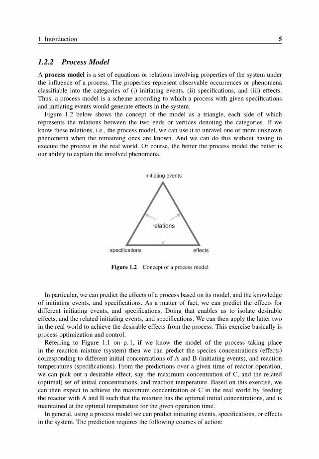
1.2.2 Process ModelA process model is a set of equations or relations involving properties of the system underthe influence of a process. The properties represent observable occurrences or phenomenaclassifiable into the categories of (i) initiating events, (ii) specifications, and (iii) effects.Thus, a process model is a scheme according to which a process with given specificationsand initiating events would generate effects in the system.

Figure 1.2 below shows the concept of the model as a triangle, each side of whichrepresents the relations between the two ends or vertices denoting the categories. If weknow these relations, i.e., the process model, we can use it to unravel one or more unknownphenomena when the remaining ones are known. And we can do this without having toexecute the process in the real world. Of course, the better the process model the better isour ability to explain the involved phenomena.

initiating events

effectsspecifications

relations

Figure 1.2 Concept of a process model

In particular, we can predict the effects of a process based on its model, and the knowledgeof initiating events, and specifications. As a matter of fact, we can predict the effects fordifferent initiating events, and specifications. Doing that enables us to isolate desirableeffects, and the related initiating events, and specifications. We can then apply the latter twoin the real world to achieve the desirable effects from the process. This exercise basically isprocess optimization and control.

Referring to Figure 1.1 on p. 1, if we know the model of the process taking placein the reaction mixture (system) then we can predict the species concentrations (effects)corresponding to different initial concentrations of A and B (initiating events), and reactiontemperatures (specifications). From the predictions over a given time of reactor operation,we can pick out a desirable effect, say, the maximum concentration of C, and the related(optimal) set of initial concentrations, and reaction temperature. Based on this exercise, wecan then expect to achieve the maximum concentration of C in the real world by feedingthe reactor with A and B such that the mixture has the optimal initial concentrations, and ismaintained at the optimal temperature for the given operation time.

In general, using a process model we can predict initiating events, specifications, or effectsin the system. The prediction requires the following courses of action:

6 Process Modeling and Simulation for Chemical Engineers

1. Process modeling – the development of a process model, and

2. Process simulation – the solution or simulation of the model, which mimics the processas it would unfold in the real world.

Types of Process Models

Process models can be categorized based on the process being represented. Thus, a steadystate model represents a steady state process, and has no time derivatives. An unsteady statemodel represents a unsteady process, and involves one or more time derivatives.

Based on the nature of system properties, a process model may be a lumped-parametermodel, or distributed-parameter model. The former involves uniform properties while thelatter has at least one property that varies with space.

Based on the type of equations involved, process models are also classified into algebraic,differential, or differential-algebraic models. Moreover, if all involved equations are linearthen the process model is called linear. Otherwise, the model is called non-linear.

1.3 Process Modeling

Process modeling is essentially an exercise that involves relating together the properties of asystem influenced by a process. Represented as mathematical symbols, the properties areassociated with each other using relevant relations under one or more assumptions. Theoutcome is a set of mathematical equations, which is a process model. The system properties –and through them, the initiating events, specifications and effects of the process – are expectedto abide by the model thus developed. The model is therefore said to represent or describe theprocess.

As an example, consider the reaction process in the reactor shown in Figure 1.1 on p. 1.The involved properties are the concentrations of A, B and C, which can be represented ascA, cB and cC, respectively, with initial values cA, cB and cC = 0. If we assume that duringthe process the reaction mixture

1. is well-mixed,

2. has constant volume, and

3. is at constant temperature

then based on certain relations, the concentrations can be associated with each other at anytime t through the following equations:

dcidt

= −r, ci(0) = ci ; i = A,B (1.1)

dcC

dt= r, cC(0) = 0 (1.2)

where r = k0 exp

(− E

RT

)caAc

bB (1.3)

1. Introduction 7

where (i) r, k0, E and T are, respectively, the rate, frequency factor, activation energy, andtemperature of the reaction, (ii) a and b are reaction-specific parameters, and (iii) R is theuniversal gas constant.

The above set of equations is the model of the reaction process taking place in the reactor.This model relates the initiating events, specifications and effects of the process with eachother [see Figure 1.2, p. 5]. The initiating events are represented by the initial concentrations,cA, cB and cC. The specifications are the values of a, b, k0, E, R and T . Finally, the processeffects at any time t, are represented by the concentrations cA(t), cB(t) and cC(t). Changesin these properties, or, equivalently, the phenomena they represent, are expected to be inaccordance with the model. Thus, for a given set of initiating events, and specifications, weexpect to find the process effects from the model.

1.3.1 Relations

Relations are the ground rules that are used in process modeling to interlink the properties ofa system under the influence of a process. These rules comprise fundamental relations basedon scientific laws, and constitutive relations. The rules manifest as equations that constituteprocess models.

A scientific law is a statement that is generally accepted to be true about one or morephenomena on the basis of repeated experiments and observations. A common example isthe law of conservation of mass. This law states that if a system does not exchange mass, orenergy (a form of mass) with the surroundings then the mass of the system stays the same, oris conserved. By applying this law to an individual species, and accounting for its generation,or consumption in a system, we derive a fundamental relation called the mass balance ofspecies.

A constitutive relation on the other hand is a rule that is true for systems with a specificmakeup or constitution. An example is Newton’s law of viscosity, which relates shear stressto strain for a system that is a Newtonian fluid.

In the model given by Equations (1.1)–(1.3) on the previous page, the last equation is aconstitutive relation. It is valid for the specific reaction mixture of species A, B and C. Thetwo differential equations are the mass balances of the species.

1.3.2 Assumptions

Assumptions of a process model are the necessary conditions that must be satisfied during theexecution of the process in order for it to be represented by the model. In equivalent terms, ifany assumption of a model is not satisfied during the execution of the process then the latteris not represented by the model.

For example, the assumptions of the model given by Equations (1.1)–(1.3) are perfectmixing, and constant volume as well as temperature. If any of these assumptions is notsatisfied during the reaction process then it would become different from the process‘assumed’ by the model, and would not be represented by the model. For instance, if mixingis not sufficiently close to perfect then there would be spatial changes in the concentrationsof species, and temperature. Consequently, the reaction process would get dominated bydiffusion, convection of species, and heat transfer, which are not accounted for by the model.

8 Process Modeling and Simulation for Chemical Engineers

The above example shows that the assumption of perfect mixing excludes from the modelthe sub-processes of diffusion, convection and heat transfer in the reaction mixture. Ingeneral, an assumption implies the exclusion of one or more sub-processes from the model.Hence, an assumption restricts the model to a specific type of process, and in doing sosimplifies the model. Note that the assumption of perfect mixing of the reaction mixturemarkedly simplifies the model by obviating the need for the diffusive fluxes of the species,and partial differential equations of momentum and heat transfer. Because of this assumption,the concentrations of species, and temperature can be considered uniform throughout thereaction mixture.

Making an assumption is justifiable under one or more of the following circumstances:

1. It is realistic to satisfy the assumption during the execution of the process.

2. Any sub-process excluded by the assumption has negligible influence on the overallprocess.

3. Without the assumption, any sub-process that should be included in the model canincrease its complexity unnecessarily.

Thus, the assumption of perfect mixing can be justified for the reaction process utilizing agood agitator that sufficiently homogenizes the reaction mixture so that the sub-processesof diffusion, convection and heat transfer can be excluded from the model. Dropping theassumption would make the model very complex. Instead it is far more practical to retain theassumption, and satisfy it by having a good agitator for the reaction process.

Remarks

An assumption limits the scope of a model by making it ignore certain sub-processes ordetails. Therefore, it follows that the fewer the assumptions the more detailed the model.A model with no assumptions would be the most comprehensive, or perfect model with nolimitations whatsoever. This of course is not possible.

As a consequence, no model can be derived without an assumption. It may be noted thatsome assumptions are implied, and not mentioned explicitly. For example, the model for thereaction process given by Equations (1.1)–(1.3) on p. 6 is based on the assumption that thereis no intermediate reaction, or product.

1.3.3 Variables and Parameters

A variable is any property that could vary with time during the execution of a process ina system. On the other hand, a parameter is a property that is fixed or specified. For thereaction process modeled by Equations (1.1)–(1.3), variables are species concentrations, andparameters are the initial concentrations, and process specifications. From the standpoint ofa process model, any symbol whose value is not fixed or specified denotes a variable. Theremaining symbols represent parameters.

Note that for a system that is not isolated, a variable, or parameter may be a property ofmass and (or) energy exchanged with the surroundings.