


Languages
Pages
Legal


HAL Id: hal-00582135https://hal.archives-ouvertes.fr/hal-00582135
Submitted on 1 Apr 2011
HAL is a multi-disciplinary open accessarchive for the deposit and dissemination of sci-entific research documents, whether they are pub-lished or not. The documents may come fromteaching and research institutions in France orabroad, or from public or private research centers.
L’archive ouverte pluridisciplinaire HAL, estdestinée au dépôt et à la diffusion de documentsscientifiques de niveau recherche, publiés ou non,émanant des établissements d’enseignement et derecherche français ou étrangers, des laboratoirespublics ou privés.
Does Tourism Influence Economic Growth? A DynamicPanel Data Approach
Tiago Neves Sequeira, Paulo Maças Nunes
To cite this version:Tiago Neves Sequeira, Paulo Maças Nunes. Does Tourism Influence Economic Growth? A DynamicPanel Data Approach. Applied Economics, Taylor & Francis (Routledge), 2008, 40 (18), pp.2431-2441.�10.1080/00036840600949520�. �hal-00582135�

For Peer Review
Does Tourism Influence Economic Growth? A Dynamic Panel Data Approach
Journal: Applied Economics
Manuscript ID: APE-06-0327.R1
Journal Selection: Applied Economics
JEL Code:
L83 - Sports|Gambling|Recreation|Tourism < L8 - Industry Studies: Services < L - Industrial Organization, O50 - General < O5 - Economywide Country Studies < O - Economic Development, Technological Change, and Growth, O40 - General < O4 - Economic Growth and Aggregate Productivity < O - Economic Development, Technological Change, and Growth
Keywords: Tourism, Economic Growth, Panel Data
Editorial Office, Dept of Economics, Warwick University, Coventry CV4 7AL, UK
Submitted Manuscript

For Peer ReviewDoes Tourism Influence Economic Growth?
A Dynamic Panel Data Approach∗
Abstract
On Average, tourism-specialized countries grow more than others. This is not
consistent with the core of modern economic growth theory that suggests that eco-
nomic growth is linked to sectors with high-tech intensity and large scale. In this
paper, we use appropriate panel data methods to study the relationship between
tourism and economic growth. In general we show that tourism is a positive deter-
minant of economic growth both in a broad sample of countries and in a sample of
poor countries. However, contrary to previous contributions, tourism is not more
relevant in small countries than in a general sample.
Key-Words: Tourism, Economic Growth, Panel Data.
JEL Classification: L83, O40, O50.
∗This is a fully modified version of a working-paper co-authored by one of the authors. We are indebtedto participants at the “Second International Conference on Tourism and Sustainable Development -Macro and Micro Issues”, supported by the World Bank, Cagliari, Italy. One of the authors also gratefullyacknowledge a financial support from the FCT, under the Project POCTI/EGE/60845/2004. The usualdisclaimer applies.
1
Page 1 of 29
Editorial Office, Dept of Economics, Warwick University, Coventry CV4 7AL, UK
Submitted Manuscript
123456789101112131415161718192021222324252627282930313233343536373839404142434445464748495051525354555657585960

For Peer Review
1 Introduction
Recently, researchers have been interested in the relationship between tourism special-
ization and economic growth, empirically supporting a direct effect from the first to the
second. However this seems to be an inconsistent fact with economic theory as, in partic-
ular, endogenous growth theory suggests that economic growth is linked with: (1) sectors
with high intensity in R&D and thus high productivity; (2) large scale. In fact, these
features are not shared by tourism-intensive countries. On the contrary, the tourism
sector is thought not to be a technologically intensive one and countries specialized in
tourism are in general small countries (see for instance Easterly and Kraay, 2000 and
Lanza and Pigliaru, 1999). Some explanations have appeared linked to a terms-of-trade
effect (Brau et al., 2003 and Copeland, 1991) and a natural resources abundance ap-
proach (Lanza and Pigliaru, 1999 and Sinclair, 1998). The first one supports that a
tourism boom tends to increase demand for non-tradable goods and this improves terms
of trade which increase growth and welfare. The second argues that tourism is linked
with the existence of renewable resources (beaches, mountains, rivers, historical and cul-
tural heritage). Thus countries with relative abundance of natural, cultural or historical
resources have comparative advantage in specializing in tourism.
An increasing number of articles have been analyzing the relationship and causality
between tourism and the economic growth rate both in specific countries (e.g. Ghali,
1974, for Hawaii; Balaguer and Jorda, 2002, for Spain; Durbarry, 2004, for Mauritius and
Gunduz and Hatemi-J, 2005 for Turkey) and in broader samples (e.g. Eugenio-Martin et
al., 2004 for Latin America). The former used standard time-series methods to conclude
that tourism had fostered growth in the specific countries studied, while the latter used a
2
Page 2 of 29
Editorial Office, Dept of Economics, Warwick University, Coventry CV4 7AL, UK
Submitted Manuscript
123456789101112131415161718192021222324252627282930313233343536373839404142434445464748495051525354555657585960

For Peer Review
dynamic panel data estimator - the differenced GMM from Arellano and Bond (1991) - to
provide evidence that the increasing number of tourists per capita caused more economic
growth in the low and medium-income countries of Latin America. The test done by Brau
et al. (2003) for a broad cross-section of countries is not robust to the possible existence
of endogeneity of tourism. Tourism may be correlated with human capital, geographic or
cultural features, for instance, and may not be an independent determinant of growth.
Thus, having data for different countries, panel data methods are the correct approach
to deal with possible endogeneity of tourism. However, due to the persistence of the
output series, Temple et. al. (2001) suggest that for a broad cross-section of countries,
one should use the System-GMM estimator from Blundell and Bond (1998).
The fact is that, on average, tourism-specialized countries grow more than others.
The next Table shows average growth rates between 1980 and 2002 for all countries for
which data are available and for subsets of countries specialized in tourism. Data are
from a panel of countries through 5 five-years periods: 1980-84, 1985-89, 1990-94, 1995-
99 and 2000-2002 and show that there is a clear positive correlation between tourism
specialization and economic growth.
Table 1: Specialization in Tourism and GrowthObservations gY
Total 1018 0.8%Specialized Countries
T/X ≥ 10% 684 1.0%T/X ≥ 25% 560 1.3%T/X ≥ 50% 521 1.5%Note: T/X measures proportion of Tourismreceipts in Exports; gY is the growth rate ofreal per capita GDP.Sources: Summers-Heston (2002) andWorld Development Indicators (2004)
In this article we employ appropriate panel data techniques that deal with endogeneity
3
Page 3 of 29
Editorial Office, Dept of Economics, Warwick University, Coventry CV4 7AL, UK
Submitted Manuscript
123456789101112131415161718192021222324252627282930313233343536373839404142434445464748495051525354555657585960

For Peer Review
(simultaneity, omitted variables, country-specific effects and measurement errors) prob-
lems and closely follow empirical growth literature to test the influence of tourism vari-
ables in economic growth in a broad panel data.1 Adding to previous literature, which
often used arrivals of tourists per capita as a proxy for tourism intensity, we also use
variables linked to the proportion of tourism in Exports and in GDP. Thus, as far as we
know, this is the first attempt to evaluate the worldwide impact of tourism, recurring to
dynamic panel data techniques that deal with endogeneity and following the empirical
economic growth literature.2 Additionally, we consider different sub-samples of countries
to test if tourism is more important for economic growth in small and poor countries,
as previous contributions argued that these sub-samples of countries should benefit more
from tourism than the average country.
In Section 2, we present data, method and variables. In Section 3, we present the
results. Section 4 concludes and motivates future research.
2 Data and Methods
2.1 Specification and Methods
We have used panel data methods to analyze this issue. The use of panel data allows not
only the increase of degrees of freedom and better estimators’ large sample properties,
but also the reduction of endogeneity, due to the consideration of specific-country effects,
omitted variables, reverse causality and measurement error.
1The use of panel data techniques in empirical economic growth literature began with Islam (1995).2This means that we study economic growth empirically through the implementation of a growth
regression that evaluates the contribution of different determinants of economic growth. The seminalarticle from Barro (1991) began this tradition.
4
Page 4 of 29
Editorial Office, Dept of Economics, Warwick University, Coventry CV4 7AL, UK
Submitted Manuscript
123456789101112131415161718192021222324252627282930313233343536373839404142434445464748495051525354555657585960

For Peer Review
We estimate the following equation:
Yi,t = α + β0Yi,t−1 + β′1CSi,t + β3tourismi,t + ηi + εi,t (1)
where Yi,t is the natural logarithm of per capita GDP at constant prices, calculated using
the chain index, CSi,t is a conditioning set that includes various covariates that previous
literature used as determinants of economic growth, tourismi,t is one of three different
measures of tourism intensity in logs, ηi is an unobserved country-specific effect and εi,t
is the error term. We have also added time dummies to all regressions.3
We present results for two different estimators: the GMM Blundell and Bond (1998)
estimator and the corrected Least Square Dummy Variables (LSDVC) or fixed effects
approach developed by Bruno (2005a, b). The essential difference is that while the first
accounts for time-varying endogenous effects and is more appropriate for large samples
(large N), the second accounts for endogeneity due to fixed-effects but is more consistent
for samples with a small number of cross-sections.
Under the assumptions that (a) the error term is not serially correlated and (b) the
explanatory variables are weakly exogenous (i.e., the explanatory variables are assumed
to be uncorrelated with future realizations of the error term), the GMM dynamic panel
uses the following moment conditions: E[Yi,t−s∆εi,t] = 0 and E[Xi,t−s∆εi,t] = 0, for s ≥
2; t = 3, ..., T ; i = 1, ..., N, where X is the complete matrix of covariates, which includes
CS and tourism. Because we use the system GMM estimator developed by Arellano and
Bover (1995) and Blundell and Bond (1998), there are the following additional moment
3In the next sub-section, we discuss the composition of the conditioning set and different measures oftourism intensity.
5
Page 5 of 29
Editorial Office, Dept of Economics, Warwick University, Coventry CV4 7AL, UK
Submitted Manuscript
123456789101112131415161718192021222324252627282930313233343536373839404142434445464748495051525354555657585960

For Peer Review
restrictions for the levels equation: E[∆Yi,t−1(ηi + εi,t)] = 0 and E[∆Xi,t−1(ηi + εi,t)] = 0,
for t = 3, ..., T.4 It is worth noting that these conditions allow for the levels of output to
be correlated with the unobserved country-specific effects. Thus, we use these moment
conditions and employ a GMM procedure to generate consistent and efficient parameter
estimates. Temple et al. (2001) argues that this estimator is appropriate to economic
growth empirical models.
Consistency of the GMM estimator depends on the validity of the instruments. To
address this issue, we consider two specification tests: the first is the Hansen test of
over-identifying restrictions, which tests the overall validity of the instruments (the null
is that the instruments are valid); the second is the second-order autocorrelation test
for the error term, which tests the null according to which there is no autocorrelation.
Overall, both specification tests indicate that the instruments used are valid (see Tables
A.1.1, A.1.2 and A.1.5 in Appendix A).
The Bruno (2005b) estimator has been shown to outperform GMM estimators in
panels with the features of this one. Monte-Carlo experiments shown in Judson and Owen
(1999) and in Bruno (2005b) indicate a corrected LSDV (Least Square Dummy Variable)
or fixed-effects estimator as better than GMM ones. In fact, in a panel with small cross-
section (due to low availability of data, total sample includes near 90 countries) and small
time-series (5 periods), GMM estimators would create many instruments, implying an
over-fitting bias.5
4This estimator is preferable to the difference estimator if the dependent variable is highly persistent,as is the case for output.
5To avoid the over-fitting bias that arises from the high number of instruments in System GMM,we restrict the number of lagged instruments to two by variable. These specification options do notchange our conclusions. In Tables A.1.1, A.1.2 and A.1.5 in Appendix A, we also present the number ofinstruments introduced in each regression. According to these numbers, we must be confident in a quitesmall “overfitting” bias. However, this would not happen in small samples for which we present results.
6
Page 6 of 29
Editorial Office, Dept of Economics, Warwick University, Coventry CV4 7AL, UK
Submitted Manuscript
123456789101112131415161718192021222324252627282930313233343536373839404142434445464748495051525354555657585960

For Peer Review
We present here the basic ideas of the estimator developed by Bruno (2005b). The
departure point is the inconsistency of LSDV in dynamic panel data models (Nickel,
1981). The approximation terms to the bias are all evaluated at the unobserved true
parameter values, which are of no direct use for estimation. Thus, to make the approx-
imation terms operational, Kiviet (1995) suggests replacing the true parameters by the
estimates from some consistent estimators. Monte Carlo experiments showed that the
resulting bias-corrected LSDV estimator (LSDVC) often outperforms IV-GMM estima-
tors in terms of bias and root mean squared error (RMSE). We use an approximation of
O(N−1T−2), which is the best approximation provided in Bruno (2005b), and we initial-
ize the estimation with the Blundell and Bond (1998) estimator. Results do not change
significantly with the choice of the consistent initial estimator, nor with the choice of the
approximation. This estimator is suitable for unbalanced panels.
2.2 Data, Variables and Conditioning Sets
2.2.1 Data on Tourism Specialization
Data on Tourism Specialization are from the World Development Indicators (World Bank,
2004) from 1980 to 2002, all time lengths available in the source. We have considered 5
five-year periods to avoid measurement errors and the effects of cycles in variables. This
is usual in empirical economic growth literature. We have considered a broad sample and
two smaller samples: Small Countries (less than an initial level of 5 million inhabitants);
Poor Countries (for which GDP per capita is below average in the majority of periods
considered). The three variables used are:
In face of this, for small samples, we present only the corrected LSDV results.
7
Page 7 of 29
Editorial Office, Dept of Economics, Warwick University, Coventry CV4 7AL, UK
Submitted Manuscript
123456789101112131415161718192021222324252627282930313233343536373839404142434445464748495051525354555657585960

For Peer Review
Tourist Arrivals as Population Proportion (TA) - The number of International inbound
tourists over population. International inbound tourists are the number of visitors
who travel to a country other than that where they have their usual residence for a
period not exceeding 12 months and whose main purpose in visiting is other than an
activity remunerated from within the country visited. This proportion is calculated
as a ratio to total population (World Bank, 2004);
Tourism receipts in % of Exports (TR1) - International tourism receipts are expendi-
tures by international inbound visitors, including payments to national carriers for
international transport. These receipts should include any other prepayment made
for goods or services received in the destination country. They also may include
receipts from same-day visitors, except in cases where these are so important as to
justify a separate classification. Their share in exports is calculated as a ratio to
exports of goods and services (World Bank, 2004);
Tourism receipts in % of GDP (TR2) - the same as the previous one but their share in
GDP is calculated using the previous variable and the ratio of exports of goods and
services to GDP (World Bank, 2004).
2.2.2 Conditioning Information Sets
To test the significance of tourism in explaining economic growth, we have used several
variables that are standard in literature (Barro, 1991 and Barro and Sala-i-Martin, 1995)
and are related to the main determinants of growth. Thus, we have used Real Gross
Domestic Product per capita in the previous period (Yi,t−1) to measure conditional con-
vergence (from which a positive sign is expected with a less-than-unity absolute value)
8
Page 8 of 29
Editorial Office, Dept of Economics, Warwick University, Coventry CV4 7AL, UK
Submitted Manuscript
123456789101112131415161718192021222324252627282930313233343536373839404142434445464748495051525354555657585960

For Peer Review
and the following Conditioning Information Set (CS1) of variables:
Investment-Output ratio (I/Y ) - is used as a proxy for physical capital investment, and
a positive sign is expected;
Government Consumption-Output ratio (G/Y ) - is used to measure long-run crowding-
out and the effect of Government Consumption in long-run growth; a negative effect
is traditionally reported, but a positive effect was shown in panel data estimations
in Caselli et al. (1996);
Secondary Years of Schooling above 25 years (Syr) - is used as a proxy for human capital;
there is a discussion in the literature about the effect of human capital; there are
positive and negative effects reported;
Life Expectancy (Life) - it is used as a proxy for health, which has been interpreted
both as a determinant of productivity and as a determinant of the savings behavior
of the households; it usually has a positive effect, but Caselli et al. (1996) reported
a non-significant effect;
Black Market Premium (1 + BMP ) - is used to measure market distortions in the
economy and the overall negative impact of institutions;
International Country Risk Guide (ICRG) - is used as an alternative measure of institu-
tions; as it is negatively related with country risk, it is expected to have a positive
relationship;6
6We note that ICRG is a more general measure for institutions than BMP because it includes 22different indicators of country risk. Nevertheless, it is less used in previous empirical contributions. Itsintroduction comes at the expense of a significant number of observations. It is increasingly used indevelopment (see e.g. the influential article of Hall and Jones, 1999).
9
Page 9 of 29
Editorial Office, Dept of Economics, Warwick University, Coventry CV4 7AL, UK
Submitted Manuscript
123456789101112131415161718192021222324252627282930313233343536373839404142434445464748495051525354555657585960

For Peer Review
As a robustness check, we have included in some regressions two additional variables
in the conditioning information set, treating the CS2 as CS1 plus the following variables:
Exports plus Imports to output ratio (Openness) - is used to measure the impact of
openness of the economy in its growth performance, and a positive sign is expected,
although this is not consensual in the literature (e.g. Edwards, 1998);
Inflation (consumer prices) (1 + π) - is used to measure the effect of high inflations in
reducing the economic growth rates (e.g. Levine et. al., 2000).
All variables except the average years of schooling are introduced as log transforma-
tions. Output, investment-output ratio, government expenditures ratio and openness are
from the Penn World Tables 6.1. Secondary Years of Schooling above 25 years comes
from Barro and Lee (2000). Life Expectancy, International Risk Country Guide, and
Inflation (consumer prices) come from the World Development Indicators 2004 (World
Bank, 2004). Black Market Premium is taken from the World Development Network
Database 2001 (World Bank, 2001).
2.2.3 Sample and Descriptive Statistics
The next table presents descriptive statistics for tourism variables. Descriptive statistics
for other variables included in the conditioning sets are presented in the Appendix.
Table 2: Descriptive StatisticsVariables Obs. Mean Std. Dev. Min. Max.GDPpc 1031 5969 6069 304.3 37689
TA 705 0.511 1.190 0 13.49TR1 744 12.04 14.84 0.055 85.60TR2 580 4.769 8.216 0.016 66.55
Note: Values for Descriptive Statistics are in levels.
10
Page 10 of 29
Editorial Office, Dept of Economics, Warwick University, Coventry CV4 7AL, UK
Submitted Manuscript
123456789101112131415161718192021222324252627282930313233343536373839404142434445464748495051525354555657585960

For Peer Review
In the next section we present the results, beginning with results for the whole sample,
and then for subsamples of small and poor countries.
3 Results
In this section we present the main results obtained. The results on the variables in the
conditioning information sets are often consistent with previous empirical literature on
economic growth. In particular, the investment ratio positively influences growth, while
the government expenditures ratio and the black market premium negatively influence
growth.
The rate of convergence oscillates around 2.44% in the System GMM estimator -
Table A.A.1, column 0 - in line with the one obtained by Temple et al. (2001) - 2.38%
in their Table 1, column (v) - and closer to OLS estimates than to the Differenced GMM
estimates of Caselli et al. (1996).7
The Influence of Life Expectancy and Schooling is almost always non-significant.
Schooling seems to be negatively related to growth in samples of small and poor coun-
tries. This is not inconsistent with previous contributions, as different results have been
reported in the literature. We have tested alternative specifications, such as the exclusion
of life expectancy and the consideration of other variables for schooling (namely average
years above 15 years old - syr15) and these changes did not change results on the sig-
nificance of the tourism variable. Nevertheless, syr15 proved to be positively related to
growth in one specification applied to the broad sample.
7As in these references, the rate of convergence λ is obtained equating e−λT to 0.885 (in the case ofcolumn 0 in Table A.1.1, Appendix A), where T = 5.
11
Page 11 of 29
Editorial Office, Dept of Economics, Warwick University, Coventry CV4 7AL, UK
Submitted Manuscript
123456789101112131415161718192021222324252627282930313233343536373839404142434445464748495051525354555657585960

For Peer Review
The impact of the inclusion of tourism in convergence is small and its direction is not
obvious, depending on the variable used. Nevertheless, the corrected LSDV estimator
predicts even a small convergence rate or no conditional convergence at all, especially in
samples of small and poor countries. In general, and in particular in the Corrected LSDV
estimations, the introduction of tourism variables acted in order to decrease significance
of other covariates, namely the impact of the government share of output (G/Y ) and the
impact of the Black Market Premium (BMP ) in poor countries.
Complete regressions are presented in Appendix, and to focus the article, we will only
be interested on the tourism effect from now on. To avoid excessive length and to focus the
article in its main issue, we are not presenting complete regressions for the conditioning
information set 2, when we use the alternative measure of institutions (ICRG). We also
present only the benchmark regressions in the small and poor countries case.8 We also
note that the specification tests in GMM indicate that instruments are valid as in general
we do not reject the null of the Hansen Test nor the null of the AR(2) test.
3.1 Results from All Countries
The next Table shows different estimators of the three variables linked with tourism
specialization in a regression with economic growth as a dependent variable.
8Although results do not influence our conclusions, they are obviously available upon request.
12
Page 12 of 29
Editorial Office, Dept of Economics, Warwick University, Coventry CV4 7AL, UK
Submitted Manuscript
123456789101112131415161718192021222324252627282930313233343536373839404142434445464748495051525354555657585960

For Peer Review
Table 3: Regressions Between Tourism and GrowthSystem GMM
tourism CS1 CS2
Institutions measure BMP ICRG BMP ICRGln(TA) 0.01 -0.02 0.03** 0.00
(1.05) (-0.82) (2.07) (0.25)ln(TR1) 0.04** 0.01 0.05*** 0.02
(2.24) (0.61) (3.13) (0.82)ln(TR2) 0.03* -0.01 0.03*** 0.01
(1.82) (-0.66) (2.64) (0.54)Corrected FE
tourism CS1 CS2
Institutions measure BMP ICRG BMP ICRGln(TA) 0.09*** 0.09*** 0.11*** 0.09***
(4.44) (3.75) (4.14) (2.62)ln(TR1) 0.05*** 0.02 0.05*** 0.02
(3.89) (1.30) (3.32) (1.50)ln(TR2) 0.04** 0.02 0.04*** 0.02
(2.48) (1.40) (2.89) (1.53)Notes: *** stands for a 1% significance level; ** for 5% and* for 10%. Regressions include several controls, constant andtime dummies. Complete Regressions are presented inAppendix (see Tables A.1.1 to A.1.6).
These results indicate that in general tourism specialization is an important deter-
minant of long-run economic growth, implying that a 1% increase in the proportion of
tourism returns on GDP (or in exports) accounts for a 0.03% to 0.05% increase in output
growth rate. Simultaneously, a 1% increase in the proportion of tourist arrivals tends to
increase near 0.1% in economic growth rate. The corrected LSDV approach attributes
a greater role to tourism than the System GMM approach. Also, when institutions are
measured by black market premium, tourism returns assume a greater role than when
institutions are measured by international country risk guide composite indicator. These
results seem to indicate that the only measure of tourism intensity that is not particularly
affected by the measure of institutions is the number of arrivals as a proportion of popu-
13
Page 13 of 29
Editorial Office, Dept of Economics, Warwick University, Coventry CV4 7AL, UK
Submitted Manuscript
123456789101112131415161718192021222324252627282930313233343536373839404142434445464748495051525354555657585960

For Peer Review
lation. Thus, bad institutions (measured as country risk) may affect the effectiveness of
returns from tourism but not the effectiveness of tourist arrivals.9
These conclusions confirm for a broad cross-section of countries observed through a
time-span of 5 five-year periods between 1980 and 2002 what has been shown for some
countries, on their own, and for groups of developing countries in previous contributions.
3.2 Results for the Sub-Samples: Small and Poor Countries
In the next Tables we show results for the small samples considered. In these small
samples we analyze the Corrected LSDV approach, as when the number of countries to
be considered decreases, this is clearly the most appropriate estimator. The first case to
be considered is the Small Countries case. We considered a country as small if it had less
than 5 million inhabitants in the first period considered. According to the explanation in
the literature, we should expect a stronger relationship within this sub-sample than in the
broad sample. According to this explanation, small countries are relatively well-endowed
with renewable natural resources and consequently benefit more from the specialization
in tourism.
9Eilat and Einov (2004), in an article on the determinants of international tourism, have discoveredthat political risk is very important to tourism.
14
Page 14 of 29
Editorial Office, Dept of Economics, Warwick University, Coventry CV4 7AL, UK
Submitted Manuscript
123456789101112131415161718192021222324252627282930313233343536373839404142434445464748495051525354555657585960
For Peer Review
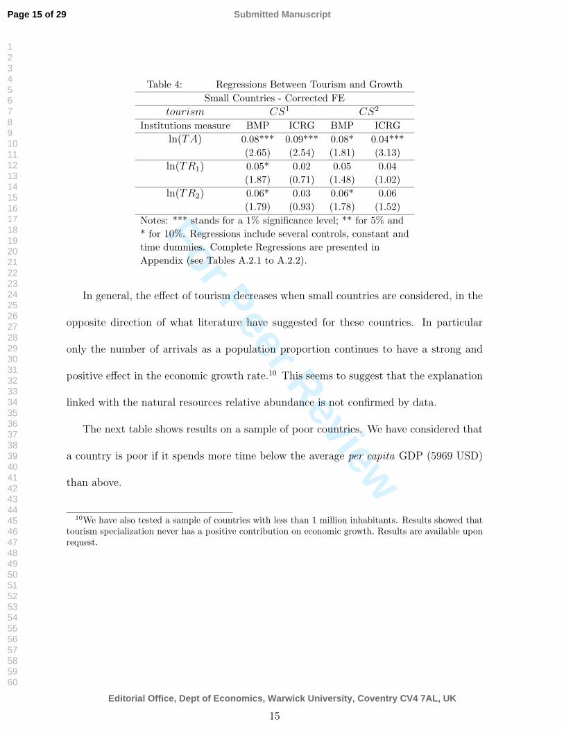
Table 4: Regressions Between Tourism and GrowthSmall Countries - Corrected FE
tourism CS1 CS2
Institutions measure BMP ICRG BMP ICRGln(TA) 0.08*** 0.09*** 0.08* 0.04***
(2.65) (2.54) (1.81) (3.13)ln(TR1) 0.05* 0.02 0.05 0.04
(1.87) (0.71) (1.48) (1.02)ln(TR2) 0.06* 0.03 0.06* 0.06
(1.79) (0.93) (1.78) (1.52)Notes: *** stands for a 1% significance level; ** for 5% and* for 10%. Regressions include several controls, constant andtime dummies. Complete Regressions are presented inAppendix (see Tables A.2.1 to A.2.2).
In general, the effect of tourism decreases when small countries are considered, in the
opposite direction of what literature have suggested for these countries. In particular
only the number of arrivals as a population proportion continues to have a strong and
positive effect in the economic growth rate.10 This seems to suggest that the explanation
linked with the natural resources relative abundance is not confirmed by data.
The next table shows results on a sample of poor countries. We have considered that
a country is poor if it spends more time below the average per capita GDP (5969 USD)
than above.
10We have also tested a sample of countries with less than 1 million inhabitants. Results showed thattourism specialization never has a positive contribution on economic growth. Results are available uponrequest.
15
Page 15 of 29
Editorial Office, Dept of Economics, Warwick University, Coventry CV4 7AL, UK
Submitted Manuscript
123456789101112131415161718192021222324252627282930313233343536373839404142434445464748495051525354555657585960

For Peer Review
Table 5: Regressions Between Tourism and GrowthPoor Countries - Corrected FE
tourism CS1 CS2
Institutions measure BMP ICRG BMP ICRGln(TA) 0.09*** 0.08** 0.10*** 0.09**
(3.45) (2.20) (3.05) (2.12)ln(TR1) 0.06*** 0.03* 0.06** 0.04*
(3.28) (1.81) (2.55) (1.89)ln(TR2) 0.05*** 0.03 0.05*** 0.03*
(2.73) (1.62) (3.00) (1.85)Notes: *** stands for a 1% significance level; ** for 5% and* for 10%. Regressions include several controls, constant andtime dummies. Complete Regressions are presented inAppendix (see Tables A.3.1 to A.3.2).
These results support the idea that tourism is an opportunity for poor countries.
In fact, almost all tourism variables are significantly and positively related to economic
growth in all specifications (the exception is proportion of tourism returns on GDP with
a positive t-ratio of 1.62). In this group of countries it is clear that the introduction of
the specialization in tourism as a determinant of economic growth decreases the influence
of the government expenditure and of the Black Market Premium.
4 Conclusion and Prospects
In general, we support the time-series evidence that has been published for a number
of countries, according to which tourism specialization enhances growth performance of
countries. We come to this conclusion using two recently developed estimators that
complement each other in terms of costs and benefits: the System GMM Blundell-Bond
(1998) estimator and the Corrected LSDV estimator developed in Bruno (2005b), and
applying them to a broad sample of countries during all the available time periods.
When testing for the two most important conclusions brought out by previous con-
16
Page 16 of 29
Editorial Office, Dept of Economics, Warwick University, Coventry CV4 7AL, UK
Submitted Manuscript
123456789101112131415161718192021222324252627282930313233343536373839404142434445464748495051525354555657585960

For Peer Review
tributions, according to which tourism specialization is important for small countries (as
small countries are relatively abundant in Natural Resources) and for poor countries, we
reject the first and confirm the second conclusion. In fact, small countries do not seem to
benefit from tourism specialization more than does the average country. On the contrary,
poor countries always benefit from tourism specialization, both in terms of arrivals and
in terms of returns. In addition, it seems that tourism specialization is a good option to
promote economic growth in poor countries, as it appears to hinder the negative effects
of government and bad institutions.
These results add to previous contributions the consideration of recent empirical meth-
ods appropriate to study economic growth. The results are generally in line with previous
time-series attempts.11 However, they question the proposition according to which small
countries benefit more from tourism than others. Finally, they emphasize the possible
contradiction between empirical results and economic growth theory regarding the rela-
tionship between growth and tourism specialization.
This opens at least two potentially fruitful research avenues. The first one is to explore
the relationship between tourism and the traditional determinants of economic growth,
e.g., human capital, both theoretically and empirically. The second one is to explore the
determinants of tourism growth and in particular to calculate the productivity within
the tourism firms. There is also a significant scope of evolution in constructing models of
economic growth that incorporate the positive influence of tourism in economic growth.
It is worth noting that establishing the relationship between tourism and economic
growth is essential concerning the importance that policy makers are attributing to this
11A first attempt to use panel data methods applied to this broad sample led to different results dueto the presence of the Nickel (1981) bias in Fixed effects estimations (see Sequeira and Campos, 2005).
17
Page 17 of 29
Editorial Office, Dept of Economics, Warwick University, Coventry CV4 7AL, UK
Submitted Manuscript
123456789101112131415161718192021222324252627282930313233343536373839404142434445464748495051525354555657585960

For Peer Review
sector and the rates at which it is growing.
References
[1] Arellano, M. and S. Bond (1991), “Some Tests of Specification for Panel Data: Monte
Carlo evidence and an Application to Employment Equations”, Review of Economic
Studies, 58: 277-297.
[2] Arellano, M. and O. Bover (1995), “Another Look at the Instrumental Variables
Estimation of Error-Components Model”, Journal of Econometrics, 68: 29-52.
[3] Balaguer, J. and M. Cantavella-Jorda (2002), “Tourism as a Long-Run Economic
Growth Factor: The Spanish Case”, Applied Economics, 34: 877-884.
[4] Barro, R. (1991), “Economic growth in a cross section of countries”, Quarterly Jour-
nal of Economics, May, vol. CVI, n. 2:407-444.
[5] Barro, R. and J. Lee (2000), International Data on Educational Attainment: Up-
dates and Implications, Working-Paper 42, Centre for International Development at
Havard University, April.
[6] Barro, R. and X. Sala-i-Martin (1995), Economic Growth, the MIT Press.
[7] Blundell, R. and S. Bond (1998), “Initial Conditions and Moment restrictions in
Dynamic Panel Data Models”, Journal of Econometrics, 87:115-143.
18
Page 18 of 29
Editorial Office, Dept of Economics, Warwick University, Coventry CV4 7AL, UK
Submitted Manuscript
123456789101112131415161718192021222324252627282930313233343536373839404142434445464748495051525354555657585960

For Peer Review
[8] Brau, R., A. Lanza, and F. Pigliaru (2003), How Fast Are The Tourism Coun-
tries Growing? The Cross Country Evidence, FEEM working paper no85.2003,
http://ssrn.com/abstract=453340.
[9] Bruno, G. (2005a), “Aproximating the Bias of LSDV estimator for Dynamic Unbal-
anced Panel Data Models”, Economics Letter, 87:361-366.
[10] Bruno, G. (2005b), “Estimation and Inference in Dynamic Unbalanced Panel Data
Models with a Small Number of Individuals”, Stata Journal, 5(4):473-500.
[11] Caselli, F., G. Gerardo and F. Lefort (1996), “Re-opening the convergence debate: a
new look at cross country growth empirics”, Journal of Economic Growth 1: 363-389.
[12] Copeland, B. (1991), “Tourism, Welfare and De-industrialization in a Small Open
Economy”, Economica, 58: 515-29.
[13] Durbarry, R. (2004), “Tourism and Economic Growth: the case of Mauritius”,
Tourism Economics, 10(4): 389-401.
[14] Easterly, W. And A. Kraay (2000), “Small States, Small Problems?” Income,
Growth and Volatility in Small States, World Development, 28: 2013-27.
[15] Edwards, S. (1998), “Openess, productivity and growth: what do we really know?”,
Economic Journal, 108: 383-398.
[16] Eilat, Y. and L. Einav (2004), “Determinants of International Tourism: a three-
dimensional panel data analysis”, Applied Economics, 36: 1315-1327.
19
Page 19 of 29
Editorial Office, Dept of Economics, Warwick University, Coventry CV4 7AL, UK
Submitted Manuscript
123456789101112131415161718192021222324252627282930313233343536373839404142434445464748495051525354555657585960

For Peer Review
[17] Eugenio-Martın, J., N. Morales and R. Scarpa (2004), Tourism and Economic
Growth in Latin American Countries: A Panel Data Approach, Nota de Lavoro
26.2004, http://ssrn.com/abstract=504482.
[18] Ghali, M. (1974), “Tourism and Economic Growth: An Empirical Study”, Economic
Development and Cultural Change, pp. 527-538.
[19] Hall, R. and C. Jones (1999), “Why do Some Countries produce so Much more
Output per Worker than Others”, Quarterly Journal of Economics, vol. 114, number
1: 83-116.
[20] Gunduz, L. and A. Hatemi-J (2005), “Is the Tourism-Led Growth Hypothesis valid
for Turkey?”, Applied Economics Letters, 12: 499-504.
[21] Islam, N. (1995), “Growth Empirics: A Panel Data Approach”, Quarterly Journal
of Economics, November, 1127-1170.
[22] Judson, R. and A. Owen (1999), “Estimating Dynamic Panel Data Models: A Guide
for Macroeconomists”, Economics Letters, 65:9-15.
[23] Kiviet, J. F. (1995), “On Bias, Inconsistency and Efficiency of Various Estimators
in Dynamic Panel Data Models”, Journal of Econometrics, 68:53-78.
[24] Lanza, A. and F. Pigliaru (1999), Why are Tourism Countries Small and Fast Grow-
ing, http://ssrn.com/abstract=146028.
[25] Levine, R., N. Loayza and T. Beck (2000), “Financial Intermediation and Growth:
Causality and Causes”, Journal of Monetary Economics, 46:31-77.
20
Page 20 of 29
Editorial Office, Dept of Economics, Warwick University, Coventry CV4 7AL, UK
Submitted Manuscript
123456789101112131415161718192021222324252627282930313233343536373839404142434445464748495051525354555657585960

For Peer Review
[26] Nickel, S. (1981), “Biases in Dynamic Models with Fixed Effects”, Econometrica,
49:1417-1426.
[27] Sequeira, T. and C. Campos (2005), International Tourism and Economic Growth:
A Panel Data Approach, Nota di Lavoro 141.2005, Fondazione Eni Enrico Mattei.
[28] Sinclair, M. (1998), “Tourism and Economic Development: a Survey”, Journal of
Development Studies, 34: 1-51.
[29] Summers, R. and A. Heston (2002), Penn World Table, Center for International
Comparisons, University of Pennsylvania.
[30] Temple, J., S. Bond and A. Hoeffler (2001), GMM Estimation of Empirical Growth
Models, Working-Paper.
[31] World Bank (2004), World Development Indicators, CD Database.
[32] World Bank (2001), World Development Network Database, World Bank On-Line.
21
Page 21 of 29
Editorial Office, Dept of Economics, Warwick University, Coventry CV4 7AL, UK
Submitted Manuscript
123456789101112131415161718192021222324252627282930313233343536373839404142434445464748495051525354555657585960

For Peer Review
A Appendix
A.1 Broad Sample
Table A.1.1: Convergence Regressions (System GMM) - CS1
Dep Var.: ln(Yi,t) (0) (1) (2) (3)ln(Yi,t−1) 0.885*** 0.873*** 0.879*** 0.918***
(29.47) (17.27) (15.33) (15.70)ln(I/Y ) 0.104*** 0.112** 0.091 0.089*
(3.73) (2.02) (1.43) (1.79)ln(G/Y ) -0.035 -0.067* -0.05 -0.074*
(-1.26) (-1.80) (-1.14) (-1.72)syr 0.026 0.016 0.049 0.014
(1.28) (0.58) (1.44) (0.45)ln(1 + BMP ) -0.022*** -0.021** -0.016* -0.022**
(-3.22) (-2.55) (-1.71) (-2.38)ln(Life) 0.284** 0.262 0.151 0.115
(2.21) (1.17) (0.65) (0.49)TA – 0.015 – –
(1.05)TR1 – – 0.043** –
(2.24)TR2 – – – 0.028*
(1.82)AR(1) Test -3.64*** -2.92*** -1.91 -2.98***(p-value) (0.000) (0.003) (0.056) (0.003)
AR(2) Test -0.82 0.15 -0.52 -1.87*(p-value) (0.414) (0.883) (0.602) (0.062)
Hansen Test 85.5 53.39 52.47 47.03(p-value) (0.289) (0.309) (0.305) (0.513)
Observations 589 334 350 312Countries 94 93 93 91
Instruments 92 59 59 59Notes: *** stands for a 1% significance level; ** for 5% and* for 10%. t-statistics based on the white heteroscedastic-consistentvariance-covariance matrix appear in parentheses.
22
Page 22 of 29
Editorial Office, Dept of Economics, Warwick University, Coventry CV4 7AL, UK
Submitted Manuscript
123456789101112131415161718192021222324252627282930313233343536373839404142434445464748495051525354555657585960

For Peer Review
Table A.1.2: Convergence Regressions (System GMM) - CS2
Dep Var.: ln(Yi,t) (0) (1) (2) (3)ln(Yi,t−1) 0.913*** 0.872*** 0.926*** 0.924***
(26.49) (17.32) (21.66) (20.62)ln(I/Y ) 0.092*** 0.092** 0.074 0.106**
(3.55) (1.96) (1.34) (2.47)ln(G/Y ) -0.029 -0.053 -0.021 -0.050
(-1.08) (-1.51) (-0.47) (-1.20)syr 0.012 0.006 0.024 0.008
(0.61) (0.26) (0.96) (0.032)ln(1 + BMP ) -0.004 0.000 -0.001 0.001
(-0.58) (0.36) (-0.17) (0.26)ln(Life) 0.290** 0.313* 0.188 0.173
(2.18) (1.80) (1.08) (0.98)ln(1 + π) -0.033*** -0.034*** -0.028*** -0.035***
(-3.32) (-4.20) (-2.82) (-4.43)ln(open) -0.018 -0.036 -0.006 -0.048*
(-0.75) (-1.20) (-0.21) (-1.69)TA – 0.031** – –
(2.07)TR1 – – 0.048** –
(3.13)TR2 – – – 0.034***
(2.69)AR(1) Test (p-value) -3.68*** -2.97*** -2.05** -2.76***
(0.000) (0.003) (0.040) (0.006)AR(2) Test (p-value) -1.23 0.39 -0.09 -1.29
(0.220) (0.698) (0.373) (0.199)Hansen Test (p-value) 83.77 62.46 73.58 64.00
(0.975) (0.601) (0.244) (0.547)Observations 532 321 336 302
Countries 94 92 93 90Instruments 124 79 79 79
Notes: *** stands for a 1% significance level; ** for 5% and* for 10%. t-statistics based on the white heteroscedastic-consistent
variance-covariance matrix appear in parentheses.
23
Page 23 of 29
Editorial Office, Dept of Economics, Warwick University, Coventry CV4 7AL, UK
Submitted Manuscript
123456789101112131415161718192021222324252627282930313233343536373839404142434445464748495051525354555657585960

For Peer Review
Table A.1.3: Convergence Regressions (Corrected FE) - CS1
Dep Var.: ln(Yi,t) (0) (1) (2) (3)ln(Yi,t−1) 1.025*** 0.870*** 1.000*** 0.932***
(17.11) (7.96) (10.34) (4.81)ln(I/Y ) 0.089*** 0.064** 0.057* 0.102***
(5.90) (2.35) (1.82) (3.56)ln(G/Y ) -0.042** -0.022 -0.004 -0.029
(-1.99) (-0.81) (-0.13) (-0.65)syr -0.024 -0.031 -0.029 -0.028
(-1.11) (-0.95) (-1.07) (-0.60)ln(1 + BMP ) -0.015*** 0.001 0.006 -0.000
(-3.27) (0.16) (-0.82) (-0.06)ln(Life) 0.163 0.289 0.367* 0.321
(0.96) (1.57) (1.95) (0.61)TA – 0.095*** – –
(4.44)TR1 – – 0.049*** –
(3.89)TR2 – – – 0.042***
(2.48)Observations 589 334 350 312
Countries 94 93 93 91Notes: *** stands for a 1% significance level; ** for 5% and* for 10%. t-statistics based on the white heteroscedastic-consistentvariance-covariance matrix appear in parentheses.
24
Page 24 of 29
Editorial Office, Dept of Economics, Warwick University, Coventry CV4 7AL, UK
Submitted Manuscript
123456789101112131415161718192021222324252627282930313233343536373839404142434445464748495051525354555657585960

For Peer Review
Table A.1.4: Convergence Regressions (Corrected FE) - CS2
Dep Var.: ln(Yi,t) (0) (1) (2) (3)ln(Yi,t−1) 1.062*** 0.891*** 1.067*** 0.954***
(27.85) (5.89) (10.12) (6.30)ln(I/Y ) 0.070*** 0.041 0.016 0.085**
(3.56) (1.40) (0.48) (2.56)ln(G/Y ) -0.026 -0.017 -0.011 -0.020
(-1.19) (-0.71) (-0.35) (-0.72)syr -0.033* -0.034 -0.039 -0.029
(-1.88) (-1.02) (-1.31) (-0.78)ln(1 + BMP ) -0.009 0.005 -0.004 0.002
(-1.61) (0.63) (-0.49) (0.26)ln(Life) 0.142 0.312 0.303 0.219
(0.92) (1.45) (1.16) (0.77)ln(1 + π) -0.024*** -0.022*** -0.016* -0.015**
(-3.24) (-3.02) (-1.85) (-2.14)ln(open) -0.030 -0.009 0.005 -0.014
(-1.55) (-0.27) (0.17) (-0.32)TA – 0.106*** – –
(4.14)TR1 – – 0.047*** –
(3.32)TR2 – – – 0.041***
(2.98)Observations 532 321 336 302
Countries 94 92 93 90Notes: *** stands for a 1% significance level; ** for 5% and* for 10%. t-statistics based on the white heteroscedastic-consistentvariance-covariance matrix appear in parentheses.
25
Page 25 of 29
Editorial Office, Dept of Economics, Warwick University, Coventry CV4 7AL, UK
Submitted Manuscript
123456789101112131415161718192021222324252627282930313233343536373839404142434445464748495051525354555657585960

For Peer Review
Table A.1.5: Convergence Regressions (System GMM) - CS1
Alternative Measure of Institutions (ICRG)Dep Var.: ln(Yi,t) (0) (1) (2) (3)
ln(Yi,t−1) 0.870*** 0.869*** 0.872*** 0.832***(16.62) (15.03) (16.17) (12.95)
ln(I/Y ) 0.155** 0.133** 0.141** 0.119**(2.15) (2.24) (2.16) (2.16)
ln(G/Y ) -0.077 -0.103** -0.088** -0.109***(-1.63) (-2.66) (-2.11) (-2.80)
syr 0.011 0.006 0.007 0.007(0.40) (0.26) (0.29) (0.22)
ln(ICRG) 0.191* 0.144 0.195** 0.139(1.84) (1.46) (2.11) (1.59)
ln(Life) 0.184 0.507** 0.200 0.605**(0.84) (2.23) (0.93) (2.48)
TA – -0.017 – –(-0.82)
TR1 – – 0.013 –(0.61)
TR2 – – – -0.013(-0.66)
AR(1) Test (p-value) -2.15** -3.13*** -1.94* -2.25**(0.031) (0.002) (0.052) (0.025)
AR(2) Test (p-value) -0.64 0.15 -0.73 -1.57(0.564) (0.880) (0.464) (0.115)
Hansen Test (p-value) 38.81 40.64 42.73 39.96(0.478) (0.574) (0.483) (0.604)
Observations 330 313 327 290Countries 87 85 86 83
Instruments 49 54 54 54Notes: *** stands for a 1% significance level; ** for 5% and* for 10%. t-statistics based on the white heteroscedastic-consistentvariance-covariance matrix appear in parentheses.
26
Page 26 of 29
Editorial Office, Dept of Economics, Warwick University, Coventry CV4 7AL, UK
Submitted Manuscript
123456789101112131415161718192021222324252627282930313233343536373839404142434445464748495051525354555657585960

For Peer Review
Table A.1.6: Convergence Regressions (Corrected FE) - CS1
Dep Var.: ln(Yi,t) (0) (1) (2) (3)ln(Yi,t−1) 0.971*** 0.898*** 0.985*** 0.959***
(6.21) (6.89) (6.42) (5.58)ln(I/Y ) 0.020 0.061** 0.015 0.095***
(0.62) (2.11) (0.45) (2.65)ln(G/Y ) -0.034 -0.049* -0.034 -0.043
(-084) (-1.74) (-0.93) (-1.39)syr -0.048 -0.040 -0.040 -0.048
(-1.23) (-1.18) (-1.31) (-1.18)ln(ICRG) 0.313*** 0.150* 0.294*** 0.190***
(3.78) (1.82) (3.83) (2.91)ln(Life) 0.059 0.228 0.119 0.116
(0.15) (0.86) (0.32) (0.33)TA – 0.087*** – –
(3.75) 0.021TR1 – – (1.30) –
TR2 – – 0.021(1.40)
Observations 330 313 327 290Countries 87 85 86 83
Notes: *** stands for a 1% significance level; ** for 5% and* for 10%. t-statistics based on the white heteroscedastic-consistentvariance-covariance matrix appear in parentheses.
27
Page 27 of 29
Editorial Office, Dept of Economics, Warwick University, Coventry CV4 7AL, UK
Submitted Manuscript
123456789101112131415161718192021222324252627282930313233343536373839404142434445464748495051525354555657585960

For Peer Review
A.2 Small Countries
Table A.2.1: Convergence Regressions (Corrected FE) - CS1
Dep Var.: ln(Yi,t) (0) (1) (2) (3)ln(Yi,t−1) 1.226*** 1.166*** 1.265*** 1.380***
(30.21) (12.27) (16.34) (12.32)ln(I/Y ) 0.068** 0.036 0.002 0.080*
(2.59) (0.90) (0.03) (1.71)ln(G/Y ) -0.057** -0.031 -0.003 -0.032
(-2.13) (-0.80) (-0.07) (-0.69)syr -0.117*** -0.141*** -0.136** -0.171***
(-3.86) (-2.88) (-2.57) (-3.47)log(1 + BMP ) -0.010 -0.005 -0.136** -0.011
(-1.33) (-0.53) (-2.57) (-0.98)ln(Life) 0.069 0.086 0.257 -0.025
(0.41) (0.43) (1.08) (-0.09)TA – 0.077*** – –
(2.65)TR1 – – 0.060* –
(1.79)TR2 – – – 0.055*
(1.87)Observations 276 159 170 149
Countries 47 47 47 45Notes: *** stands for a 1% significance level; ** for 5% and* for 10%. t-statistics based on the white heteroscedastic-consistentvariance-covariance matrix appear in parentheses.
28
Page 28 of 29
Editorial Office, Dept of Economics, Warwick University, Coventry CV4 7AL, UK
Submitted Manuscript
123456789101112131415161718192021222324252627282930313233343536373839404142434445464748495051525354555657585960

For Peer Review
A.3 Poor Countries
Table A.3.1: Convergence Regressions (Corrected FE) - CS1
Dep Var.: ln(Yi,t) (0) (1) (2) (3)ln(Yi,t−1) 1.133*** 1.013*** 1.096*** 1.052***
(40.40) (9.20) (11.62) (8.75)ln(I/Y ) 0.079*** 0.054 0.038 0.093***
(4.45) (1.54) (0.94) (2.79)ln(G/Y ) -0.076*** -0.006 0.034 -0.030
(-3.07) (-0.11) (0.67) (-0.60)syr -0.090*** -0.081* -0.076 -0.092**
(-2.99) (-1.73) (-1.52) (-2.03)log(1 + BMP ) -0.017*** -0.001 -0.006 0.003
(-3.00) (-0.07) (-0.59) (0.25)ln(Life) 0.172 0.220 0.387 0.292
(1.32) (0.85) (1.35) (0.89)TA – 0.092*** – –
(3.45)TR1 – – 0.063*** –
(3.28)TR2 – – – 0.055***
(2.73)Observations 376 206 222 195
Countries 59 58 58 58Notes: *** stands for a 1% significance level; ** for 5% and* for 10%. t-statistics based on the white heteroscedastic-consistent
variance-covariance matrix appear in parentheses.
B Descriptive Statistics for Variables in CS1 and CS2
Table B.1: Descriptive StatisticsVariables Obs. Mean Std. Dev. Min. Max.ln(I/Y ) 1039 2.54 0.70 -0.04 3.92ln(G/Y ) 1039 2.89 0.58 0.96 5.02
syr 940 1.20 1.13 0.01 5.09ln(1 + BMP ) 963 2.16 1.89 -1.05 10.84
ln(Life) 1536 4.09 0.22 3.46 4.40ln(Open) 1041 4.00 1.02 -19.26 5.84ln(1 + π) 1075 2.24 1.24 -3.80 8.80ln(ICRG) 605 4.11 0.26 2.93 4.56
29
Page 29 of 29
Editorial Office, Dept of Economics, Warwick University, Coventry CV4 7AL, UK
Submitted Manuscript
123456789101112131415161718192021222324252627282930313233343536373839404142434445464748495051525354555657585960
Top Related